1 3

Exp Fluids (2016) 57:33DOI 10.1007/s00348-015-2110-8

RESEARCH ARTICLE

Adaptive vector validation in image velocimetry to minimise the influence of outlier clusters

Alessandro Masullo1 · Raf Theunissen1

Received: 8 July 2015 / Revised: 21 December 2015 / Accepted: 22 December 2015 / Published online: 17 February 2016 © The Author(s) 2016. This article is published with open access at Springerlink.com

validation routine is applied to the PIV analysis of experi-mental studies focused on the near wake behind a porous disc and on a supersonic jet, illustrating the potential gains in spatial resolution and accuracy.

1 Introduction

Particle image velocimetry (PIV) is a mature measurement technique whereby flow-induced displacement of tracer particles between sequential image recordings is deduced by means of statistical operators. The most common of these operators is cross-correlation (Keane and Adrian 1992). Although versatile, the robustness and accuracy of correlation are strongly influenced by image quality, nota-bly image noise and particle image density, and underlying flow features such as velocity gradients (Westerweel 2008) and flow curvature (Scarano 2004). An insufficient number of particle images to constitute a traceable pattern or too strong a distortion of the particle image pattern between snapshots can lead to erroneous velocity estimates. Incor-rect vectors in turn severely penalise the iterative image analysis process and the computation of derivative quanti-ties (Etabari and Vlachos 2005), while further deteriorating measurement uncertainty. Vector outlier detection has con-sequently received considerable attention within the PIV community resulting in a variety of detection schemes.

Song et al. (1999), for example, identify spurious vec-tors on the basis of continuity in the aforementioned pat-tern deformation adopting Delaunay tessellation. However, a simpler and more commonly applied approach to discern an erroneous displacement vector in the post-processing stage is through its mismatched appearance with respect to neighbouring vectors. This can be either along the tem-poral and/or spatial dimension. In the former, even for

Abstract The universal outlier detection scheme (Wester-weel and Scarano in Exp Fluids 39:1096–1100, 2005) and the distance-weighted universal outlier detection scheme for unstructured data (Duncan et al. in Meas Sci Technol 21:057002, 2010) are the most common PIV data valida-tion routines. However, such techniques rely on a spatial comparison of each vector with those in a fixed-size neigh-bourhood and their performance subsequently suffers in the presence of clusters of outliers. This paper proposes an advancement to render outlier detection more robust while reducing the probability of mistakenly invalidating correct vectors. Velocity fields undergo a preliminary evaluation in terms of local coherency, which parametrises the extent of the neighbourhood with which each vector will be com-pared subsequently. Such adaptivity is shown to reduce the number of undetected outliers, even when implemented in the afore validation schemes. In addition, the authors present an alternative residual definition considering vec-tor magnitude and angle adopting a modified Gaussian-weighted distance-based averaging median. This procedure is able to adapt the degree of acceptable background fluctu-ations in velocity to the local displacement magnitude. The traditional, extended and recommended validation methods are numerically assessed on the basis of flow fields from an isolated vortex, a turbulent channel flow and a DNS simula-tion of forced isotropic turbulence. The resulting validation method is adaptive, requires no user-defined parameters and is demonstrated to yield the best performances in terms of outlier under- and over-detection. Finally, the novel

* Alessandro Masullo a.masullo@bristol.ac.uk

1 Department of Aerospace Engineering, University of Bristol, Bristol, UK

Exp Fluids (2016) 57:33

1 3

33 Page 2 of 21

non-time-resolved PIV data, proper orthogonal decomposi-tion (POD) has been implemented as a filter (Wang et al. 2015; Raiola et al. 2015) or one resorts to more statistical approaches (Griffin et al. 2010). Intermediate outlier detec-tion in iterative image processing sequences can, however, only rely on spatial information. Artificial neural net-works have been proposed to evaluate the interconnection between individual vectors in the instantaneous velocity field (Liang et al. 2003). A more straightforward prediction of the model vector is based on the local median of a 3 × 3 neighbourhood, followed by imposing a fixed, uniform threshold on the residual between the scrutinised vector and estimator (Westerweel 1994). To relax the limitation of a spatially invariant threshold, Raffel et al. (1992) imple-mented an adaptive threshold utilising a local velocity vari-ability based on the moving average of the vectors. Wester-weel and Scarano (2005) constructed a reliable and robust threshold adopting a normalised median threshold (hereaf-ter referred to as NMT); the difference between a correct vector and its estimator, which is based on the neighbour-hood median, must fall within two times the median of the discrepancy between the neighbouring vectors and the pre-diction. Though widely applied, Duncan et al. (2010) high-light this approach to be unsuitable for unstructured data such as in particle tracking velocimetry (PTV) or adaptive PIV routines (Theunissen et al. 2007) and should include a weighting inversely proportional to the distance between vectors. This technique will be referred to as DW-NMT.

Both NMT and DW-NMT approaches have been cate-gorically demonstrated to identify isolated outliers even if local median tests may suffer from under- and over-detec-tion (Lecuona et al. 2002). The former refers to failing to detect an outlier. Especially in the presence of clusters of erroneous vectors, the augmented fluctuation level causes the normalised threshold to be on a par with correct vec-tors. These faulty vectors are subsequently wrongly con-sidered correct. Clustering of outliers is a quite common problem in PIV due to low seeding areas or strong light reflections on surfaces for instance, and the inherent prob-lematic for validation is worth the attention. Over-detection refers to the case of classifying correct vectors as errone-ous, which is prone in the presence of strong velocity gra-dients. To minimise this sensitivity, Nogueira et al. (1997) iteratively discriminated outliers on the basis of a valida-tion criterion utilising predictions from interpolations con-sidering the eight nearest vectors assessed to be coherent. Coherency was quantified as the ratio between the mean residual and the mean magnitude. This solution was shown to minimise the overall influence of outliers in data valida-tion in the form of a reduced ratio between root mean value of the error and displacement, but at the cost of complexity. Moreover, as stated by the authors the method would fail in the presence of outlier clusters and continued the need

of defining an appropriate validation threshold. The lat-ter has been addressed by Shinneeb et al. (2004) through the implementation of a spatially varying threshold. Prior to evaluating the residual between the measured vector and the prediction, potential outliers are identified using a median filter and replaced with a distance-based Gaussian-weighted average. After adding a user-defined constant, the filtered discrepancy serves as a heuristic for the local median test. This approach yielded promising results in terms of reducing over- and under-detection despite the continuing need of refinement of the introduced constant. To further mitigate over-detection, Young et al. (2004) dis-tinguish between spurious vectors and variations due to local velocity gradients by incorporating a local thin-plate spline model to which vectors are compared. By adjusting the degree of smoothness in the spline model and the vec-tor removal criterion, over-detection could be diminished in the presence of significant velocity gradients.

In this paper, the authors present a novel adaptive vec-tor validation algorithm capable of (1) detecting clusters of outliers, (2) reducing the degree of over-detection, (3) over-coming the restrictions of existing methodologies by negat-ing user input and (4) safeguarding computational simplic-ity. Although the process still applies the concept of median normalised thresholds, three ideas are introduced which elaborate on the findings of the studies mentioned afore. First, the number of neighbours for comparison is adjusted based on local flow coherency. The latter is quantified by means of second-order regression. The authors argue that clusters of outliers are characterised by a higher variance (randomness) and the size of the vector basis for compari-son must be extended accordingly. This step renders the validation algorithm fully adaptive. Second, an average-weighted median is introduced to reduce over-detections by relaxing the importance of distant data sites. Third, erroneous vectors are defined as local anomalies in vector direction and magnitude, whereas traditionally validation is based on the Cartesian velocity components. The authors would like to stress that the current work does not inves-tigate the appropriate method of outlier replacement. The interested reader can find further information in relevant references such as Nogueira et al. (1997), Garcia (2011), Raben et al. (2012) and Sciacchitano et al. (2012).

After illustrating the problematic surrounding outlier identification, the suggested methodology is explained in Sect. 3. Section 4 concerns the assessment on the basis of benchmark velocity fields contaminated with synthetic spu-rious vectors. Appreciable amelioration in under- and over-detection is demonstrated. Incorporation of the adaptive neighbourhood is also shown to be a very efficient concept to decrease the number of under-detections when applied to the traditional techniques. The improved validation pro-cess is finally incorporated in a recursive multi-grid image

Exp Fluids (2016) 57:33

1 3

Page 3 of 21 33

analysis routine and applied to the experimental wake of a porous disc and supersonic jet in Sect. 5.

2 Problem statement: coherency

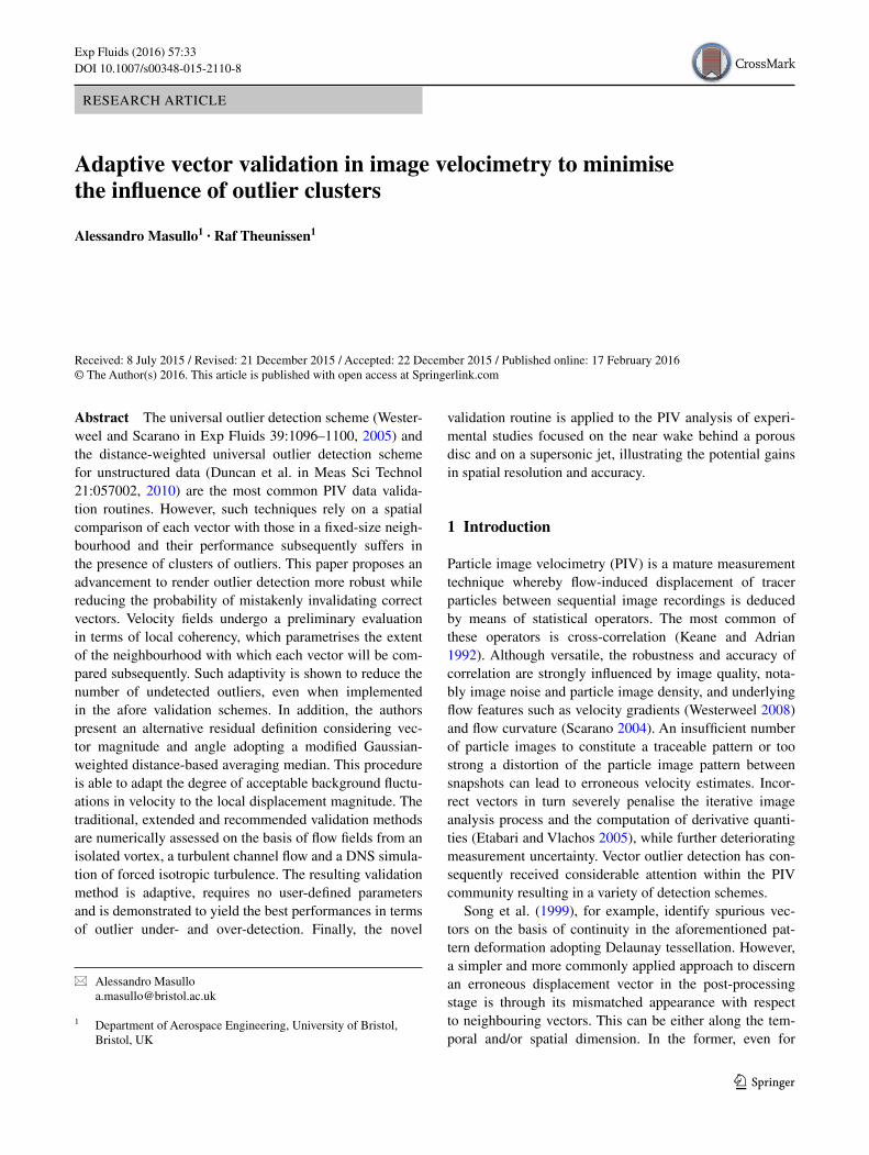
Human vision is considered the best tool in the identification of outliers, and its strength lies in the cognitive ability to dis-tinguish coherent structures (Reiz and Pongor 2011). Each vector is unconsciously juxtaposed with its closest neigh-bours, and this basis for comparison is extended until a rec-ognisable pattern emerges providing sufficient reliability to discriminate outliers. This process is illustrated in Fig. 1. The small collection of vectors in Fig. 1a could be deemed inva-lid if only the local neighbourhood were to be considered. However, extending the neighbourhood it becomes clear the vectors form part of either a coherent structure (Fig. 1b) or outlier cluster (Fig. 1c). While classic spatial outlier detec-tion methodologies consult a restricted vicinity of typically eight (3 × 3-1) to 24 (5 × 5-1) vectors, the example high-lights the need to adaptively expand the locality as to emu-late human vision. Simultaneously, a group of actual outliers should not influence the validation process in such a manner as to invalidate correct outliers (over-detection).

Prior to validating a vector, an appropriate neighbour-hood extent must therefore be selected. The methods of Nogueira et al. (1997) and Shinneeb et al. (2004) both incorporate an initial consistency heuristic to specify the basis for vector comparison in the following process stage. However, neither method accounts for the adverse effect of velocity gradients in coherent structures. As depicted in Fig. 1, both methods conjecture several correct elements of the vector collection as incoherent. A majority of vectors may consequently be invalidated already in the prepara-tory stage and excluded or replaced successively. Either approach inherently neglects underlying flow physics and

essentially filters measured data, thereby influencing the overall accuracy of the results. Instead, in the current work the authors argue that each vector should be considered valid from the outset and coherency should only dictate the extent of the proximity to take into account. Reminis-cent of the typical decay in spatial velocity correlations a weighting inversely proportional with spacing must then be applied to reflect the influence of each comparative vector. Differentiation between vectors must thus take place at a later stage with care to minimise the effect of outliers. Such an approach will greatly reduce the percentage of over-detection, irrespective of the degree of vector accumulation.

Concerning the validation criteria, these are most com-monly based on velocity component magnitudes. These magnitudes are attributed an acceptable fluctuation level during validation (Westerweel and Scarano 2005), which is assimilated with the typical RMS level ε of 0.1 pixels in dis-placement data. A simple graphical representation in Fig. 2a indicates that this can lead to validation of vectors which are sufficiently different. More importantly, this disparity increases as the vector magnitude decreases (Fig. 2b) neces-sitating a variable background fluctuation level proportional to the vector magnitude. On the other hand, imposing such adaptive fluctuation levels εα in the angular direction while allowing tangential fluctuations of ε shows a promising reduction in potential vector disparity (Fig. 2c–d). Such val-idation criteria are in line with the observation of Reiz and Pongor (2011) that human vision mainly identifies anoma-lies in patterns based on deviations in angle and magnitude.

3 Methodology

This paper addresses the problematic of over- and under-detection when validating PIV and PTV data. To account for spatially varying vector densities and flow properties,

Fig. 1 Illustration of the need for adaptive neighbourhood selection in vector validation. a Detail of vectors echoing outli-ers. Scrutinised vectors are bold. Only by expanding the local neighbourhood does it become clear these vectors belong to b a valid flow structure or c outlier cluster. Symbols in b indicate which vectors are consid-ered incoherent based on the values of (Σi|Vi|)

−1∙(Σi|Vi − Vo|) according to Nogueira et al. (1997) (blue circle) and the median test of Shinneeb et al. (2004) (red triangle)

Exp Fluids (2016) 57:33

1 3

33 Page 4 of 21

an adaptive validation process with a three-tiered structure is proposed (Fig. 3). The problem of under-detected outli-ers due to their aggregation in clusters is settled through a comparison of vectors with a variable number of neigh-bours based on flow coherence. Over-detection is dealt with by different improvements; an average Gaussian-weighted distance-based median estimation and a revised calcula-tion of vector discrepancy. The starting point of the lat-ter is the local median concept (Westerweel and Scarano 2005) because of its demonstrated robustness. In the cur-rent work, the authors alter the residual calculation on the basis of vector orientation and magnitude and implement an adaptive estimation of the acceptable level of reminis-cent noise-induced velocity fluctuations. The proposed methodology thus consolidates an adaptive weighted angle and magnitude threshold and will be referred to with the abbreviation AWAMT.

3.1 Coherence adaptive neighbourhood level

To define the required number of neighbouring vectors, the authors introduce a heuristic for coherency. The authors argue that the condition for a vector to be considered coher-ent is its agreement with a second-order surface fitted to its eight closest neighbours. It is important to underline that this coherence function is not used to discern correct vec-tors from outliers. Coherency is only used to predict the number of neighbours to be taken into account when esti-mating the local true flow velocity.

The choice of a quadratic surface is selected assimilat-ing the common Q-parameter to identify and visualise coherent structures (Hunt et al. 1988). Adopting the Ein-stein summation convention, Q values are calculated as

Q = −0.5(∂ui/∂xj∙∂uj/∂xi). Imposing a surface of the form Φ = a0 + a1y + a2x + a3xy + a4y

2 + a5x2 for the veloc-

ity components will thus ensure all Q isosurfaces to be also second-order continuous. To minimise the influence of outliers on the parabolic regression, a diagonal matrix W is implemented containing Gaussian weights utilising the deviation σj of each vector from the local median (includ-ing all 9 vectors) as argument; W(j + 1,j + 1) = exp(−½∙σj

2∙κj−2) where j = 0…8, σj

2 = (uj − um)2 + (vj − vm)2, um = median(uj), vm = median(vj) and κj = ε + 1

9Σσj. The

coefficients of the parabolic surface fitted to the components of the nine vectors are then estimated in a least-squares manner; a = (XTWX)−1(XTWf) where a = [a0 a1 … a5]

T, f = [(u,v)j], X = [1 yj xj xjyj yj

2 xj2].

The coherence C is subsequently quantified as the aver-age residual between the scrutinised vector’s components u0 and v0 and Φu,v evaluated at the vector’s location (x0,y0), normalised with the median of the vector magnitudes |V|m and background error ε (Westerweel and Scarano 2005);

The differentiation between coherent and non-coherent vectors is thereon done by thresholding; values of C infe-rior to the threshold T are classified as coherent. Although the threshold T can be adjusted to reflect the sensitivity of the number of neighbours to the size of clusters, the authors found performances to be relatively unaffected by the choice of T and a threshold of 10 % was empirically found by the authors to yield a reliable and generally robust selec-tion criterion.

Once the coherence function has been evaluated for all the data points in the vector field, the level of neighbour-hood L for each data point is progressively increased con-sidering the neighbours of the neighbours until at least half of the basis for comparison comprises coherent vectors. Note that L as such is a spatially varying parameter. To

(1)

C = Cu+Cv

2with C(u,v) = 1

(|V |m+ε)2(Φ(u,v)(x0, y0)

− (u0, v0))2

and |V |m = median

(

(

u2j + v2j

)0.5)

Fig. 2 Acceptable vector vari-ations for a fluctuation level ε in a both horizontal and vertical velocity components u and v, respectively, for larger and b small vector magnitudes. Limits in variations with adaptive angle variations εα for c large and d small vector magnitudes

Fig. 3 Three steps in adaptive vector validation, based on a metric for vector coherency; the number of vectors in the local vicinity is increased to provide a reliable basis for subsequent outlier detection

Exp Fluids (2016) 57:33

1 3

Page 5 of 21 33

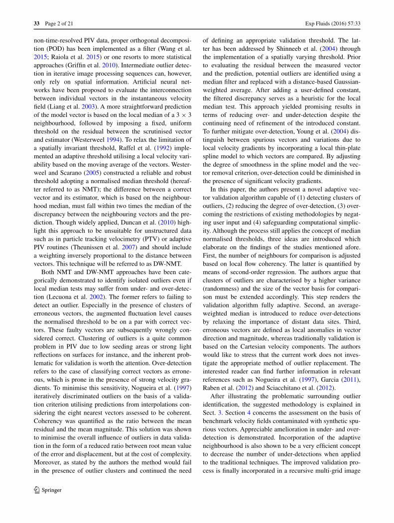
account for vector dependency due to correlation window overlap WOR, a minimum value for L is imposed which depends on WOR; Lmin = Round(4∙WOR). In the case of a structured grid for example, the total number of neigh-bours No is readily given as No = (2L + 3)2 − 1 (Fig. 4a). This stopping criterion ensures the median of an examined neighbourhood will return a reliable and coherent predic-tion for ensuing validation purposes since at least half the considered adjoining vectors are deemed coherent. The coherency check accordingly addresses the effects of under- and over-detection in the presence of outlier clusters and is straightforward to implement in existing validation routines.

Figure 4b illustrates the outcome of the coherency test when a cluster of outliers is surrounded by coher-ent vectors. The local neighbourhood level gradually increases towards the centre of the cluster, as indicated by the greyscale, such that each outlier can be compared with a reliable prediction even when surrounded by outliers.

3.2 Adaptive angle and magnitude median normalised residual

While the methodology presented above will be shown to already improve standard validation processes, the authors implement two additional modifications to the traditional normalised residual calculation to further lessen the num-ber of over-detections: (1) average Gaussian-weighted median estimation and (2) comparison of direction and magnitude instead of Cartesian vector components. The underlying principle still remains consistent with com-mon detection routines; a normalised residual is evaluated for each vector of the field based on the fluctuation of its neighbours and is used to discern correct vectors from outliers.

• Average-weighted median estimation

To identify the scrutinised vector as being erroneous, a comparison is required with an adequate estimation of the true, underlying flow vector. Such a prediction is ideally based on interpolation of neighbouring vectors. Because of the fundamental sensitivity of interpolation to the presence of spurious vectors, the median offers a more robust alter-native. Following the selection of an adequate neighbour-hood level based on coherency, a distance-based weighting is introduced when calculating a vector prediction from the No vectors to reflect their relative importance. While still inversely proportional with spacing di between the central vector located at (xo,yo) and those in the constrained vicin-ity, in the current paper the weights wi are drawn from a Gaussian functional in line with adaptive Gaussian win-dowing (AGW) with optimal filter width σ (Agui and Jimé-nez 1987);

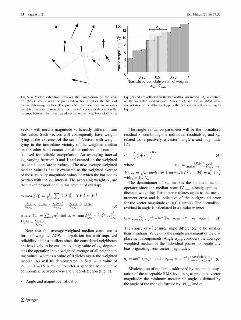
To achieve an efficiency of the statistical estimator higher than that of the weighted median, an averaging is introduced. The resulting average-weighted median opera-tion will be symbolised in the following by awmed(∙). The concept of this novel process is illustrated considering the velocity magnitude, i.e. awmed(|V|), for the situation in Fig. 5a where the central vector is adjoined by No neigh-bours (here No = 8). The No velocity magnitudes (indi-cated by the vertical abscissa location of the ● symbols) are sorted in ascending order |V|S with the corresponding weights wS, attributed according to Eq. (2), represented by the bar widths in Fig. 5b. The weighted median (solid vertical line) is located at half the cumulative sum Sw,No of the weights wS per its definition. To classify as an outlier,

(2)wi = exp(

−d2iσ 2

)

with σ = 1.24No

No∑

i=1

di

Fig. 4 a Incremental neigh-bourhood level with Lmin = 0 in case of a vector placement on the nodes of a structured grid. b Illustration of the automatic evaluation of the required neighbourhood level L indicated by the greyscale. The central area of the flow field has been artificially contaminated with outliers. Towards the centre of the cluster, the level increases indicative of strongly incoher-ent vectors necessitating an enlarged number of vectors for validation

Exp Fluids (2016) 57:33

1 3

33 Page 6 of 21

vectors will need a magnitude sufficiently different from this value. Such vectors will consequently have weights lying at the extremes of the set wS. Vectors with weights lying in the immediate vicinity of the weighted median on the other hand cannot constitute outliers and can thus be used for reliable interpolation. An averaging interval Δw varying between 0 and 1 and centred on the weighted median is therefore introduced. The new, average-weighted median value is finally evaluated as the weighted average of those velocity magnitude values of which the bar widths overlap with the Δw interval. The averaging weights λi are then taken proportional to this amount of overlap;

where Sw,i =∑i

j=1 wSj and �i = min(

Sw,iSw,No

− 1−∆w

2,

wSi

Sw,No,

1+∆w

2− Sw,i−1

Sw,No).

Note that this average-weighted median constitutes a form of weighted AGW interpolation but with improved reliability against outliers since the considered neighbours are less likely to be outliers. A unity value of Δw degener-ates the operation into a weighted average of all neighbour-ing values, whereas a value of 0 yields again the weighted median. As will be demonstrated in Sect. 4, a value of Δw = 0.3–0.5 is found to offer a generically conducive compromise between over- and under-detection (Fig. 8).

• Angle and magnitude validation

(3)

awmed(|V |) = 1∑

�i

∑

i�i|V |Si ∀|V |Si ∈ |V |S

∣

∣

∣

Sw,iSw,No

≥ 1−∆w

2∧ Sw,i−wS

i

Sw,No= Sw,i−1

Sw,No≤ 1+∆w

2

The single validation parameter will be the normalised residual r* combining the individual residuals rα and r|V| related to, respectively, a vector’s angle α and magnitude |V|;

where r|V | = ||Vo|−|V |awm|median(||V |j−|V |awm|)+ε

,

|V |awm =√

awmed(uj)2 + awmed(vj)2 and |V|j2 = uj

2 + v2j with j = 1…No

The denominator of r|V| invokes the standard median operator since the median norm |V|awm already applies a distance weighting. Parameter ε relates again to the meas-urement error and is indicative of the background error for the vector magnitude (ε ≈ 0.1 pixels). The normalised residual in angle is calculated in a similar manner;

The choice of αj* ensures angle differences to be smaller

than π radians. Value αj is the simple arc-tangent of the dis-placement components. Angle αawm considers the average-weighted median of the individual phases to negate any bias originating from vector magnitudes;

Misdetection of outliers is addressed by automatic adap-tation of the acceptable RMS level in αj to predicted vector magnitude; the minimum measurable angle is defined by the angle of the triangle formed by |V|awm and ε;

(4)r∗ =(

r2α + r2|V |

)0.5

(5)rα = α∗omedian(α∗j )+εα

α∗j = min

(∣

∣αj − αawm∣

∣, 2π − |αj − αawm|)

(6)αj = tan−1(vj/uj) and αawm = tan−1(awmed(sin(αj))

awmed(cos(αj)))

Fig. 5 a Vector validation involves the comparison of the cen-tral (black) vector with the predicted vector (grey) on the basis of the neighbouring vectors. The prediction follows from an average-weighted median. b Weights in the awmed(∙) operator depend on the distance between the investigated vector and its neighbours following

Eq. (2) and are reflected in the bar widths. An interval Δw is centred on the weighted median (solid black line), and the weighted aver-age is taken of the data overlapping the defined interval according to Eq. (3)

Exp Fluids (2016) 57:33

1 3

Page 7 of 21 33

Once the normalised residual has been evaluated throughout the vector field, r* values below a threshold of 2 are considered non-valid. This value is in agreement with the findings of Westerweel and Scarano (2005) and Duncan et al. (2010).

• Computational effort

The selection of the adequate neighbourhood level and the evaluation of the average-weighted median can be expected to come with some computational overhead. To estimate the increase in processing time as a result of the elaborated vector validation, the evaluation of the experi-mental images discussed in further detail in Sect. 5 is considered. The total processing time for the porous disc recordings with AWAMT increased by a factor of 1.01 rela-tive to the traditional NMT. Similarly, the ratio in compu-tation time between NMT and AWAMT for the analysis of the 280 image recordings related to the supersonic jet equalled 1.05. Stand-alone, the proposed validation based on magnitude and angle, although strongly dependent on flow type, number of outliers and clustering factor, was approximately four times more computationally intense compared to the standard routine based on Cartesian com-ponents. The above heuristics are only exemplary and per-tinent to the current test cases. Nevertheless, results imply the computational expense of the more elaborate AWAMT method to be marginal relative to the overall process and will be shown to be outweighed by the achievable improve-ment in measurement accuracy in the remainder of this paper.

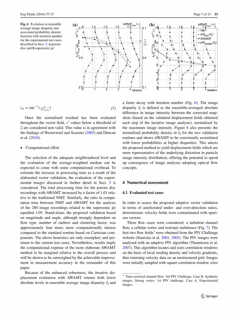
Because of the enhanced robustness, the iterative dis-placement evaluation with AWAMT returns both lower absolute levels in ensemble average image disparity δI and

(7)εα = tan−1( ε|V |awm )

a faster decay with iteration number (Fig. 6). The image disparity δI is defined as the ensemble-averaged absolute difference in image intensity between the corrected snap-shots (based on the validated displacement fields obtained each step of the iterative image analysis), normalised by the maximum image intensity. Figure 6 also presents the normalised probability density in δI for the two validation routines and shows AWAMT to be consistently assimilated with lower probabilities at higher disparities. This attests the proposed method to yield displacement fields which are more representative of the underlying distortion in particle image intensity distribution, offering the potential to speed up convergence of image analyses adopting optical flow concepts.

4 Numerical assessment

4.1 Evaluated test cases

In order to assess the proposed adaptive vector validation in terms of ameliorated under- and over-detection ratios, deterministic velocity fields were contaminated with spuri-ous vectors.

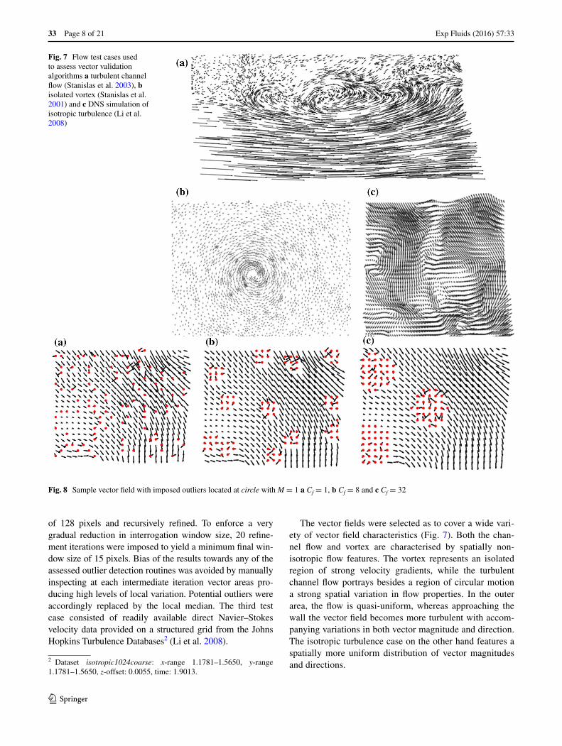
Three flow cases were considered: a turbulent channel flow, a cellular vortex and isotropic turbulence (Fig. 7). The first two flow fields1 were obtained from the PIV Challenge website (Stanislas et al. 2001, 2003). The PIV images were analysed with an adaptive PIV algorithm (Theunissen et al. 2007). This algorithm locates and sizes correlation windows on the basis of local seeding density and velocity gradients, thus returning velocity data on an unstructured grid. Images were initially sampled with square correlation window sizes

1 Time-resolved channel flow: 3rd PIV Challenge, Case B, Synthetic images. Strong vortex: 1st PIV challenge, Case A, Experimental images.

Fig. 6 Evolution in ensemble average image disparity and associated probability density function with iteration number for the experimental test cases described in Sect. 5: a porous disc and b supersonic jet

Exp Fluids (2016) 57:33

1 3

33 Page 8 of 21

of 128 pixels and recursively refined. To enforce a very gradual reduction in interrogation window size, 20 refine-ment iterations were imposed to yield a minimum final win-dow size of 15 pixels. Bias of the results towards any of the assessed outlier detection routines was avoided by manually inspecting at each intermediate iteration vector areas pro-ducing high levels of local variation. Potential outliers were accordingly replaced by the local median. The third test case consisted of readily available direct Navier–Stokes velocity data provided on a structured grid from the Johns Hopkins Turbulence Databases2 (Li et al. 2008).

2 Dataset isotropic1024coarse: x-range 1.1781–1.5650, y-range 1.1781–1.5650, z-offset: 0.0055, time: 1.9013.

The vector fields were selected as to cover a wide vari-ety of vector field characteristics (Fig. 7). Both the chan-nel flow and vortex are characterised by spatially non-isotropic flow features. The vortex represents an isolated region of strong velocity gradients, while the turbulent channel flow portrays besides a region of circular motion a strong spatial variation in flow properties. In the outer area, the flow is quasi-uniform, whereas approaching the wall the vector field becomes more turbulent with accom-panying variations in both vector magnitude and direction. The isotropic turbulence case on the other hand features a spatially more uniform distribution of vector magnitudes and directions.

Fig. 7 Flow test cases used to assess vector validation algorithms a turbulent channel flow (Stanislas et al. 2003), b isolated vortex (Stanislas et al. 2001) and c DNS simulation of isotropic turbulence (Li et al. 2008)

Fig. 8 Sample vector field with imposed outliers located at circle with M = 1 a Cf = 1, b Cf = 8 and c Cf = 32

Exp Fluids (2016) 57:33

1 3

Page 9 of 21 33

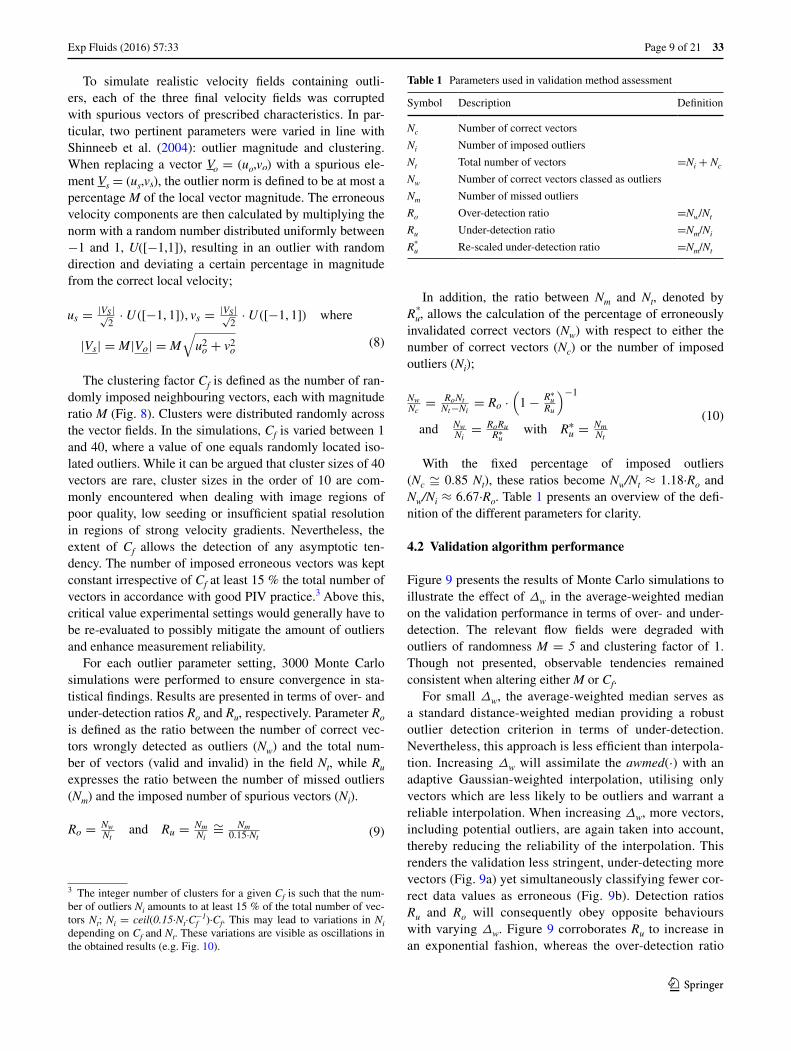
To simulate realistic velocity fields containing outli-ers, each of the three final velocity fields was corrupted with spurious vectors of prescribed characteristics. In par-ticular, two pertinent parameters were varied in line with Shinneeb et al. (2004): outlier magnitude and clustering. When replacing a vector Vo = (uo,vo) with a spurious ele-ment Vs = (us,vs), the outlier norm is defined to be at most a percentage M of the local vector magnitude. The erroneous velocity components are then calculated by multiplying the norm with a random number distributed uniformly between −1 and 1, U([−1,1]), resulting in an outlier with random direction and deviating a certain percentage in magnitude from the correct local velocity;

The clustering factor Cf is defined as the number of ran-domly imposed neighbouring vectors, each with magnitude ratio M (Fig. 8). Clusters were distributed randomly across the vector fields. In the simulations, Cf is varied between 1 and 40, where a value of one equals randomly located iso-lated outliers. While it can be argued that cluster sizes of 40 vectors are rare, cluster sizes in the order of 10 are com-monly encountered when dealing with image regions of poor quality, low seeding or insufficient spatial resolution in regions of strong velocity gradients. Nevertheless, the extent of Cf allows the detection of any asymptotic ten-dency. The number of imposed erroneous vectors was kept constant irrespective of Cf at least 15 % the total number of vectors in accordance with good PIV practice.3 Above this, critical value experimental settings would generally have to be re-evaluated to possibly mitigate the amount of outliers and enhance measurement reliability.

For each outlier parameter setting, 3000 Monte Carlo simulations were performed to ensure convergence in sta-tistical findings. Results are presented in terms of over- and under-detection ratios Ro and Ru, respectively. Parameter Ro is defined as the ratio between the number of correct vec-tors wrongly detected as outliers (Nw) and the total num-ber of vectors (valid and invalid) in the field Nt, while Ru expresses the ratio between the number of missed outliers (Nm) and the imposed number of spurious vectors (Ni).

(8)

us = |VS |√2· U([−1, 1]), vs = |VS |√

2· U([−1, 1]) where

|Vs| = M|Vo| = M

√

u2o + v2o

3 The integer number of clusters for a given Cf is such that the num-ber of outliers Ni amounts to at least 15 % of the total number of vec-tors Nt; Ni = ceil(0.15∙Nt∙Cf

−1)∙Cf. This may lead to variations in Ni depending on Cf and Nt. These variations are visible as oscillations in the obtained results (e.g. Fig. 10).

(9)Ro = Nw

Ntand Ru = Nm

Ni

∼= Nm

0.15·Nt

In addition, the ratio between Nm and Nt, denoted by Ru

*, allows the calculation of the percentage of erroneously invalidated correct vectors (Nw) with respect to either the number of correct vectors (Nc) or the number of imposed outliers (Ni);

With the fixed percentage of imposed outliers (Nc ≅ 0.85 Nt), these ratios become Nw/Nt ≈ 1.18∙Ro and Nw/Ni ≈ 6.67∙Ro. Table 1 presents an overview of the defi-nition of the different parameters for clarity.

4.2 Validation algorithm performance

Figure 9 presents the results of Monte Carlo simulations to illustrate the effect of Δw in the average-weighted median on the validation performance in terms of over- and under-detection. The relevant flow fields were degraded with outliers of randomness M = 5 and clustering factor of 1. Though not presented, observable tendencies remained consistent when altering either M or Cf.

For small Δw, the average-weighted median serves as a standard distance-weighted median providing a robust outlier detection criterion in terms of under-detection. Nevertheless, this approach is less efficient than interpola-tion. Increasing Δw will assimilate the awmed(·) with an adaptive Gaussian-weighted interpolation, utilising only vectors which are less likely to be outliers and warrant a reliable interpolation. When increasing Δw, more vectors, including potential outliers, are again taken into account, thereby reducing the reliability of the interpolation. This renders the validation less stringent, under-detecting more vectors (Fig. 9a) yet simultaneously classifying fewer cor-rect data values as erroneous (Fig. 9b). Detection ratios Ru and Ro will consequently obey opposite behaviours with varying Δw. Figure 9 corroborates Ru to increase in an exponential fashion, whereas the over-detection ratio

(10)

Nw

Nc= RoNt

Nt−Ni= Ro ·

(

1− R∗uRu

)−1

andNw

Ni= RoRu

R∗uwith R∗

u = Nm

Nt

Table 1 Parameters used in validation method assessment

Symbol Description Definition

Nc Number of correct vectors

Ni Number of imposed outliers

Nt Total number of vectors =Ni + Nc

Nw Number of correct vectors classed as outliers

Nm Number of missed outliers

Ro Over-detection ratio =Nw/Nt

Ru Under-detection ratio =Nm/Ni

Ru* Re-scaled under-detection ratio =Nm/Nt

Exp Fluids (2016) 57:33

1 3

33 Page 10 of 21

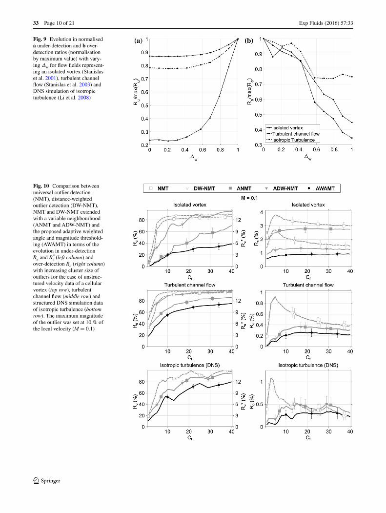
Fig. 9 Evolution in normalised a under-detection and b over-detection ratios (normalisation by maximum value) with vary-ing Δw for flow fields represent-ing an isolated vortex (Stanislas et al. 2001), turbulent channel flow (Stanislas et al. 2003) and DNS simulation of isotropic turbulence (Li et al. 2008)

Fig. 10 Comparison between universal outlier detection (NMT), distance-weighted outlier detection (DW-NMT), NMT and DW-NMT extended with a variable neighbourhood (ANMT and ADW-NMT) and the proposed adaptive weighted angle and magnitude threshold-ing (AWAMT) in terms of the evolution in under-detection Ru and Ru

* (left column) and over-detection Ro (right column) with increasing cluster size of outliers for the case of unstruc-tured velocity data of a cellular vortex (top row), turbulent channel flow (middle row) and structured DNS simulation data of isotropic turbulence (bottom row). The maximum magnitude of the outlier was set at 10 % of the local velocity (M = 0.1)

Exp Fluids (2016) 57:33

1 3

Page 11 of 21 33

shows a quasi-linear decline. Given that the depicted tendencies are quasi-flow-case independent, the authors propose a value of Δw = 0.3–0.5 as a generally con-ducive compromise to minimise both the under- and over-detection.

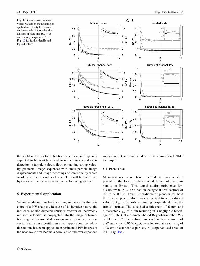
Figures 10, 11 and 12 present the under- and over-detec-tion ratios defined in Eq. (9) with varying sizes of outlier clusters for the three flow cases when fixing the magnitude ratios M, respectively, to 0.1, 1 and 10. Results of the new algorithm (AWAMT) are juxtaposed with the NMT (West-erweel and Scarano 2005) and DW-NMT method (Dun-can et al. 2010). To stress the importance of the adaptivity introduced in the current work, both methodologies have been extended to include the coherency test and automati-cally select the adequate number of neighbours in the vali-dation process. These extended routines are annotated as ANMT and ADW-NMT, respectively. Although cluster sizes Cf were incremented in steps of one, data symbols are depicted sporadically to retain figure clarity.

Independent of the considered flow case, all figures substantiate the detrimental influence of outlier clusters.

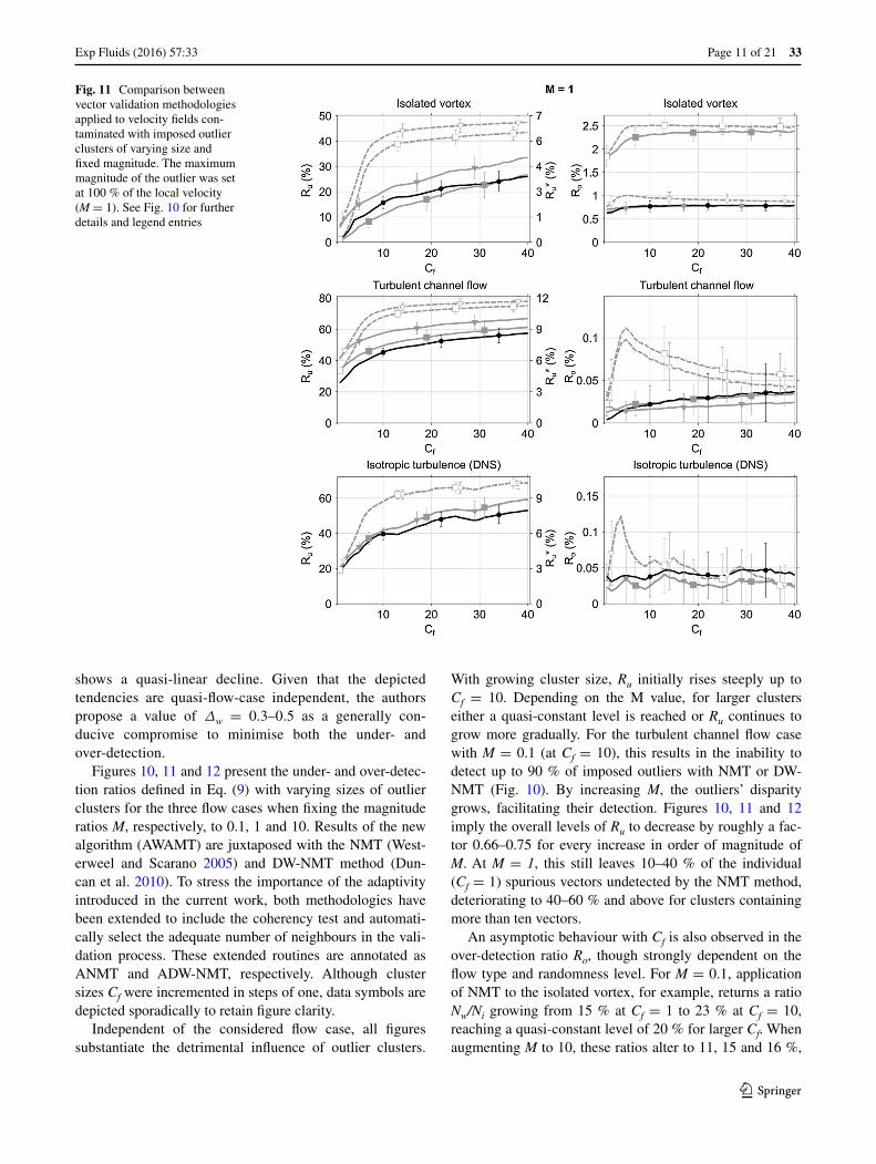
With growing cluster size, Ru initially rises steeply up to Cf = 10. Depending on the M value, for larger clusters either a quasi-constant level is reached or Ru continues to grow more gradually. For the turbulent channel flow case with M = 0.1 (at Cf = 10), this results in the inability to detect up to 90 % of imposed outliers with NMT or DW-NMT (Fig. 10). By increasing M, the outliers’ disparity grows, facilitating their detection. Figures 10, 11 and 12 imply the overall levels of Ru to decrease by roughly a fac-tor 0.66–0.75 for every increase in order of magnitude of M. At M = 1, this still leaves 10–40 % of the individual (Cf = 1) spurious vectors undetected by the NMT method, deteriorating to 40–60 % and above for clusters containing more than ten vectors.

An asymptotic behaviour with Cf is also observed in the over-detection ratio Ro, though strongly dependent on the flow type and randomness level. For M = 0.1, application of NMT to the isolated vortex, for example, returns a ratio Nw/Ni growing from 15 % at Cf = 1 to 23 % at Cf = 10, reaching a quasi-constant level of 20 % for larger Cf. When augmenting M to 10, these ratios alter to 11, 15 and 16 %,

Fig. 11 Comparison between vector validation methodologies applied to velocity fields con-taminated with imposed outlier clusters of varying size and fixed magnitude. The maximum magnitude of the outlier was set at 100 % of the local velocity (M = 1). See Fig. 10 for further details and legend entries

Exp Fluids (2016) 57:33

1 3

33 Page 12 of 21

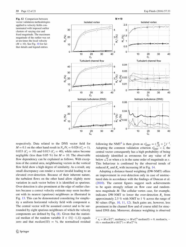
respectively. Data related to the DNS vector field for M = 0.1 on the other hand result in Nw/Ni = 0.026 (Cf = 1), 0.033 (Cf = 10) and 0.013 (Cf = 40), while ratios become negligible (less than 0.05 %) for M = 10. The observable flow dependency can be explained as follows. With excep-tion of the central area, neighbouring vectors in the vortical flow field show a high degree of similarity. As a result, any small discrepancy can render a vector invalid leading to an elevated over-detection. Because of their inherent nature, the turbulent flows on the other hand allow slightly more variation in each vector before it is identified as spurious. Over-detection is also prominent at the edge of outlier clus-ters because a correct velocity estimate may seem incoher-ent with its nearest (spurious) neighbours as illustrated in Fig. 13. This can be demonstrated considering for simplic-ity a uniform horizontal velocity field with component u. The central vector will be assumed correct and to be sur-rounded by eight spurious neighbours of which the velocity components are defined by Eq. (8). Given that the statisti-cal median of the random variable X ∈ U([−1,1]) equals zero and that median(|X|) = ½, the normalised residual

following the NMT4 is then given as r∗NMT = ( M√8+ ε

u)−1.

Adopting the common validation criterion r∗NMT < 2, the central vector consequently has a high probability of being mistakenly identified as erroneous for any value of M below

√2 or when u is in the same order of magnitude as ε.

This behaviour is confirmed by the observed trends of reduced Ro and Ru with increasing M in Fig. 14.

Adopting a distance-based weighting (DW-NMT) offers an improvement in over-detection only in case of unstruc-tured data in accordance with the findings of Duncan et al. (2010). The current figures suggest such achievements to be again strongly reliant on flow case and random-ness magnitude M. The cellular vortex case, for example, indicates DW-NMT to lower the over-detection Ro from approximately 2.5 % with NMT to 1 % across the range of M values (Figs. 10, 11, 12). Such gains are, however, less prominent in the channel flow and of course nihil for struc-tured DNS data. Moreover, distance weighting is observed

4 ui = M∙u∙X/2½, median(ui) = M∙u/2½∙median(X) = 0, median(|ui − 0|) = median(M∙u∙|X|/2½) = M∙u/2½∙½.

Fig. 12 Comparison between vector validation methodologies applied to velocity fields con-taminated with imposed outlier clusters of varying size and fixed magnitude. The maximum magnitude of the outlier was set at ten times the local velocity (M = 10). See Fig. 10 for fur-ther details and legend entries

Exp Fluids (2016) 57:33

1 3

Page 13 of 21 33

to adversely address under-detection as related Ru values are consistently higher or at least on a par with NMT, even in case of isolated spurious vectors (Cf = 1).

The presented results advocate the beneficial impact when implementing an adaptive neighbourhood extent (exemplified in Fig. 13) in NMT and DW-NMT. At low M, under-detection can be abated by roughly a factor 1.5; when applied to the wall turbulent flow field for exam-ple, for a cluster of ten vectors Ru drops from 90 to 65 % and from 80 to 65 % in case of the DNS flow (Fig. 10). Improvements become most remarkable at higher levels of randomness where Ru is lowered by at least a factor 4, from 30 to 7 % at Cf = 10 and M = 10 for the chan-nel flow and from 20 to 4 % for the DNS case (Fig. 12). Betterment is also achieved in Ro as a result of the added adaptivity, though the relative improvement drops with higher M values. Irrespective of cluster size, coherency adaptivity lowers the NMT-related Ro level. At M = 1 for example by 0.1 % for the vortex field and 0.01 % for the channel flow, whereas for M = 0.1 the differences in the vortex flow amount to 1 % when Cf = 5 and 0.3 % when Cf = 40. Maintaining a constant cluster size of eight vec-tors and varying the outlier randomness further corrobo-rates the neighbourhood adaptivity to attain under- and over-detection levels sufficiently below those of the stand-ard approaches (Fig. 14). Under-detection ratios of tradi-tional validation routines asymptotically reach values of 20 % with increasing M compared to levels approaching 0 % when implementing adaptivity. For the case of the iso-lated vortex, NMT retains 2 % over-detection, whereas the original and extended DW-NMT and AWAMT reach levels below 0.8 %. This is an important finding as it implies tra-ditional validation routines are, contrary to those enhanced with adaptivity, unable to identify all spurious vectors within the cluster, independent of their magnitude. While appreciable gains can be achieved in Ru, all validation

methods reach comparable asymptotic values in over-detection when applied to more turbulent flows.

Validation on the basis of residuals in magnitude and orientation allows the AWAMT approach proposed within this work to further reduce over- and under-detections. As per the simplistic mathematical model discussed afore, potential advantages will be particularly noticeable at lower M and displacement magnitudes in the order of one pixel or below. Figure 10 advocates the adaptation of the back-ground fluctuation level in vector phase to its magnitude to offer noticeable improvements particularly at M = 0.1. Across the various flow fields, AWAMT consistently yields the lowest Ru and Ro levels compared to the standard and enhanced median threshold techniques. Under-detection levels are overall lessened by roughly 10 % compared to the improved ANMT and ADW-NMT. Changes in Ro are flow dependent but vary between 0.15 and 0.3 %. With increasing M, relative improvements obtained by adding the magnitude and angle validation diminish compared to the benefit of purely a varying neighbourhood.

To summarise, the performed assessment has shown the traditional NMT and DW-NMT to be highly sensi-tive to the presence of outlier clusters especially in terms of under-detection. Although over-detection is prominent in the vicinity of such clusters, it is strongly dependent on the local level of velocity fluctuation and lowers as ran-domness increases. By adapting the considered neighbour-hood level to local flow coherency, under-detection can be improved considerably in the case of large outlier clusters and strong spatial velocity variations, while gains in over-detection are most noticeable with smaller displacements. Further improvements in under- and over-detection are achieved by adapting the validation process to consider vector magnitude and orientation, whereby ameliorations are particularly noticeable in case of smaller displacements. Incorporation of an adaptive weighted angle and magnitude

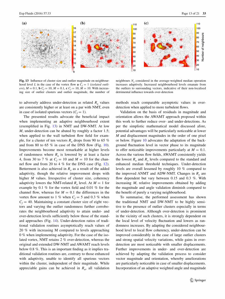
Fig. 13 Influence of cluster size and outlier magnitude on neighbour-hood level L in the case of the vortex flow a Cf = 1 (isolated outli-ers), M = 0.1, b Cf = 10, M = 0.1, c Cf = 10, M = 10. With increas-ing size of outlier clusters and outlier magnitude, the number of

neighbours No considered in the average-weighted median operation increases adaptively. Increased neighbourhood levels emanate from the outliers to surrounding vectors, indicative of their non-localised detrimental influence towards over-detection

Exp Fluids (2016) 57:33

1 3

33 Page 14 of 21

threshold in the vector validation process is subsequently expected to be most beneficial to reduce under- and over-detection in turbulent flows, flows containing strong veloc-ity gradients, image sequences with small particle image displacements and image recordings of lower quality which would give rise to outlier clusters. This will be confirmed by the experimental assessment in the following section.

5 Experimental application

Vector validation can have a strong influence on the out-come of a PIV analysis. Because of its iterative nature, the influence of non-detected spurious vectors or incorrectly replaced velocities is propagated into the image deforma-tion stage with associated consequences. To assess the new vector validation algorithm in a real application, the adap-tive routine has been applied to experimental PIV images of the near-wake flow behind a porous disc and over-expanded

supersonic jet and compared with the conventional NMT technique.

5.1 Porous disc

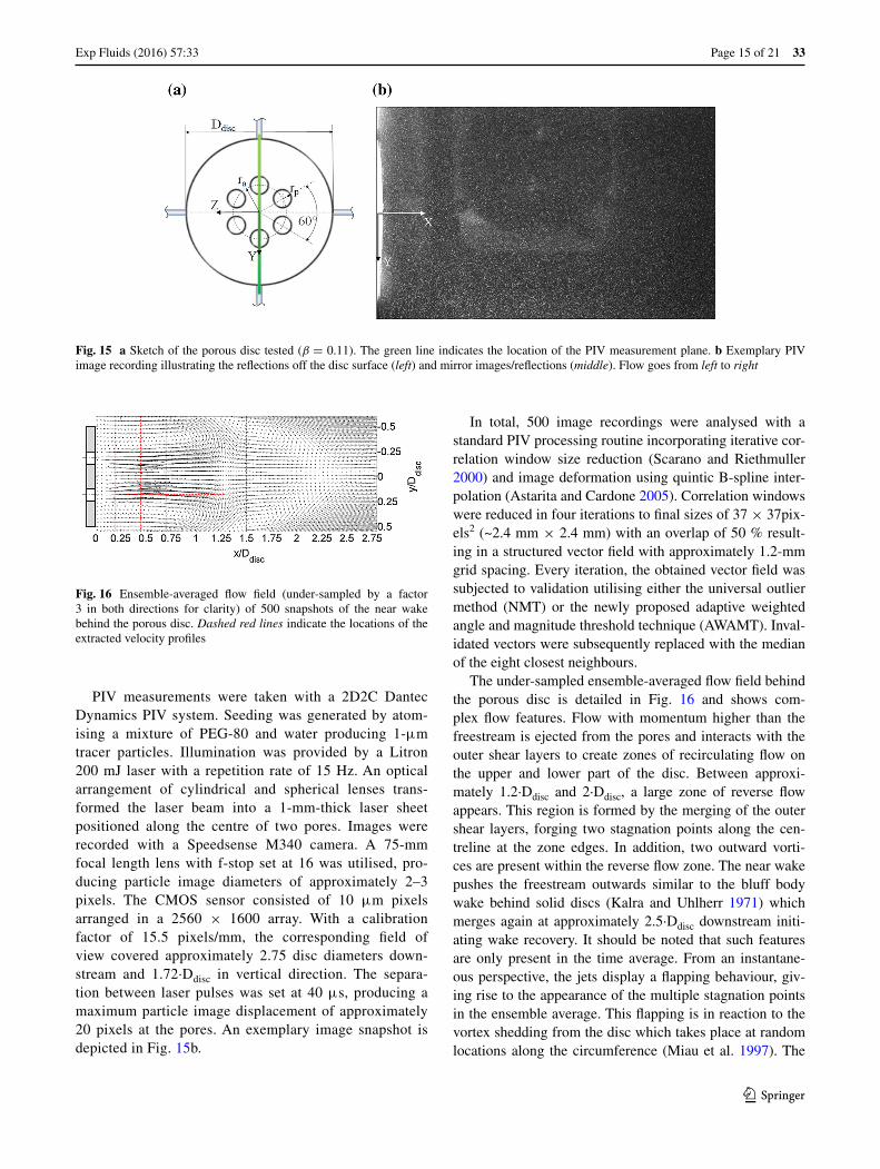
Measurements were taken behind a circular disc placed in the low turbulence wind tunnel of the Uni-versity of Bristol. This tunnel attains turbulence lev-els below 0.05 % and has an octagonal test section of 0.8 m × 0.6 m. Four 3-mm-diameter piano wires held the disc in place, which was subjected to a freestream velocity Ufs of 30 m/s impinging perpendicular to the frontal surface. The disc had a thickness of 6 mm and a diameter Ddisc of 6 cm resulting in a negligible block-age of 0.16 % at a diameter-based Reynolds number ReD of 11.6 × 104. Six perforations, each with a radius rp of 3.87 mm (rp ≈ 0.065∙Ddisc), were located at a radius ra of 1.08 cm to establish a porosity β (=open/closed area) of 0.11 (Fig. 15a).

Fig. 14 Comparison between vector validation methodologies applied to velocity fields con-taminated with imposed outlier clusters of fixed size (Cf = 8) and varying magnitude. See Fig. 10 for further details and legend entries

Exp Fluids (2016) 57:33

1 3

Page 15 of 21 33

PIV measurements were taken with a 2D2C Dantec Dynamics PIV system. Seeding was generated by atom-ising a mixture of PEG-80 and water producing 1-μm tracer particles. Illumination was provided by a Litron 200 mJ laser with a repetition rate of 15 Hz. An optical arrangement of cylindrical and spherical lenses trans-formed the laser beam into a 1-mm-thick laser sheet positioned along the centre of two pores. Images were recorded with a Speedsense M340 camera. A 75-mm focal length lens with f-stop set at 16 was utilised, pro-ducing particle image diameters of approximately 2–3 pixels. The CMOS sensor consisted of 10 μm pixels arranged in a 2560 × 1600 array. With a calibration factor of 15.5 pixels/mm, the corresponding field of view covered approximately 2.75 disc diameters down-stream and 1.72∙Ddisc in vertical direction. The separa-tion between laser pulses was set at 40 μs, producing a maximum particle image displacement of approximately 20 pixels at the pores. An exemplary image snapshot is depicted in Fig. 15b.

In total, 500 image recordings were analysed with a standard PIV processing routine incorporating iterative cor-relation window size reduction (Scarano and Riethmuller 2000) and image deformation using quintic B-spline inter-polation (Astarita and Cardone 2005). Correlation windows were reduced in four iterations to final sizes of 37 × 37pix-els2 (~2.4 mm × 2.4 mm) with an overlap of 50 % result-ing in a structured vector field with approximately 1.2-mm grid spacing. Every iteration, the obtained vector field was subjected to validation utilising either the universal outlier method (NMT) or the newly proposed adaptive weighted angle and magnitude threshold technique (AWAMT). Inval-idated vectors were subsequently replaced with the median of the eight closest neighbours.

The under-sampled ensemble-averaged flow field behind the porous disc is detailed in Fig. 16 and shows com-plex flow features. Flow with momentum higher than the freestream is ejected from the pores and interacts with the outer shear layers to create zones of recirculating flow on the upper and lower part of the disc. Between approxi-mately 1.2∙Ddisc and 2∙Ddisc, a large zone of reverse flow appears. This region is formed by the merging of the outer shear layers, forging two stagnation points along the cen-treline at the zone edges. In addition, two outward vorti-ces are present within the reverse flow zone. The near wake pushes the freestream outwards similar to the bluff body wake behind solid discs (Kalra and Uhlherr 1971) which merges again at approximately 2.5∙Ddisc downstream initi-ating wake recovery. It should be noted that such features are only present in the time average. From an instantane-ous perspective, the jets display a flapping behaviour, giv-ing rise to the appearance of the multiple stagnation points in the ensemble average. This flapping is in reaction to the vortex shedding from the disc which takes place at random locations along the circumference (Miau et al. 1997). The

Fig. 15 a Sketch of the porous disc tested (β = 0.11). The green line indicates the location of the PIV measurement plane. b Exemplary PIV image recording illustrating the reflections off the disc surface (left) and mirror images/reflections (middle). Flow goes from left to right

Fig. 16 Ensemble-averaged flow field (under-sampled by a factor 3 in both directions for clarity) of 500 snapshots of the near wake behind the porous disc. Dashed red lines indicate the locations of the extracted velocity profiles

Exp Fluids (2016) 57:33

1 3

33 Page 16 of 21

flapping in addition gives rise to mobile zones of turbu-lence and accompanying velocity gradients, making the flow a challenging test case for vector validation.

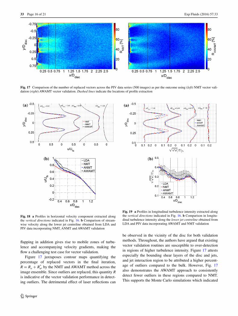
Figure 17 juxtaposes contour maps quantifying the percentage of replaced vectors in the final iteration, R = Ro + Ru

*, by the NMT and AWAMT method across the image ensemble. Since outliers are replaced, this quantity R is indicative of the vector validation performance in detect-ing outliers. The detrimental effect of laser reflections can

be observed in the vicinity of the disc for both validation methods. Throughout, the authors have argued that existing vector validation routines are susceptible to over-detection in regions of higher turbulence intensity. Figure 17 attests especially the bounding shear layers of the disc and jets, and jet interaction region to be attributed a higher percent-age of outliers compared to the bulk. However, Fig. 17 also demonstrates the AWAMT approach to consistently detect fewer outliers in these regions compared to NMT. This supports the Monte Carlo simulations which indicated

Fig. 17 Comparison of the number of replaced vectors across the PIV data series (500 images) as per the outcome using (left) NMT vector vali-dation (right) AWAMT vector validation. Dashed lines indicate the locations of profile extraction

Fig. 18 a Profiles in horizontal velocity component extracted along the vertical directions indicated in Fig. 16. b Comparison of stream-wise velocity along the lower jet centreline obtained from LDA and PIV data incorporating NMT, ANMT and AWAMT validation

Fig. 19 a Profiles in longitudinal turbulence intensity extracted along the vertical directions indicated in Fig. 16. b Comparison in longitu-dinal turbulence intensity along the lower jet centreline obtained from LDA and PIV data incorporating AWAMT and NMT validation

Exp Fluids (2016) 57:33

1 3

Page 17 of 21 33

AWAMT to abate the number of undetected outliers and lower the number of over-detections. In the shear lay-ers of the jets exiting from the perforations for example, NMT invalidates 60 % of the vectors compared to 30 % by AWAMT. In the outer shear layers, AWAMT lowers the number of replaced outliers on average from 30 to 15 %.

The advantage of coherence adaptivity in terms of meas-urement accuracy is highlighted in Figs. 18 and 19 where ensemble-averaged profiles in horizontal velocity and longitudinal turbulence obtained with NMT, ANMT and AWAMT are juxtaposed. Despite the higher uncertainty in second-order statistics as a result of the limited number of velocity fields, tendencies in differences between the validation methods will prevail and can be used to quali-tatively assess performances. While velocity profiles at x/Ddisc = 0.2 are on a par in the regions |y/Ddisc| < 0.1 and |y/Ddisc| > 0.25, a larger disparity between the validation methodologies can be observed in jet centreline velocities. Whereas ANMT and AWAMT yield a peak velocity ratio of approximately 1.05 and 1.1, respectively, NMT predicts a ratio of approximately 0.8. The observed modulation in jet velocity thus shows a strong correlation with R as the inherent vector re-interpolation will introduce a smooth-ening effect. The coherence adaptivity in ANMT and AWAMT reduces over-detection and limits the assimilated modulation, corroborating the importance of the proposed adaptivity process. Travelling downstream, the two pore jets increase in width and the centrelines arc inwards to merge at x/Ddisc = 0.7 similar to well-documented paral-lel jet theory (Anderson and Spall 2001). Velocity gradients gradually reduce in strength and validation based on vec-tor magnitude and direction becomes less stringent, caus-ing ANMT and AWAMT to attain nigh equal results. An underestimation of the jet centreline velocity obtained with NMT remains noticeable; 0.64 for AWAMT and ANMT compared to 0.61 with NMT at x/Ddisc ≈ 0.7.

To provide an estimate of the underlying true flow field, PIV data extracted along y/Ddisc = 0.18 are superim-posed with results obtained from a two-component Dan-tec Dynamics Laser Doppler Anemometry (LDA) system operating in crossed beam mode (Fig. 18b). The LDA measurement volume extended approximately 0.17 mm (~0.0028∙Ddisc) in streamwise normal direction providing spatially highly resolved measurement data. Because of the inherent beam alignment measurements closest to the disc were restricted to 0.3 disc diameters. Velocity samples were spaced approximately 0.017∙Ddisc up to 1.3 diameters downstream. At each measurement, location velocity statis-tics were evaluated on the basis of typically 6000 instanta-neous samples sampled at 4 kHz from which the depicted error bars at 95 % confidence level were inferred. Error bars for PIV data are not depicted in the figures as they

scale directly with the LDA data by a factor √12, which is

based on the number of independent data samples.The observable tendency in LDA data confirms veloc-

ity exiting from the pores can surpass the freestream condi-tion, suggesting the holes to act as contractions. Towards the disc, the magnitude of the average LDA horizontal velocity component is seen to exceed the PIV data which is caused by the bias of the PIV data towards lower veloci-ties. In vertical direction, the flow emitted from the pore decreases from nearly freestream conditions to reverse flow over approximately half the pore diameter, equating to a velocity gradient du/dy ~ 0.37 pixels/pixel. It is well known that such magnitudes in velocity gradient are challenging for any PIV image analysis (Westerweel 2008) and veloci-ties will be biased towards lower values as supported by the observations. Given its small interrogation volume and by weighting velocity data by the corresponding transit times, LDA velocity data will suffer to a much lesser extent from such a bias (Gould and Loseke 1993). As substantiated by Fig. 18, in the region 0.3 ≤ x/Ddisc < 0.9 where RNMT > RAW-

AMT, NMT yields the lowest velocity values in comparison with AWAMT, advocating the improved accuracy of the lat-ter. Incorporating coherence adaptivity clearly enhances the accuracy of the ensemble average velocity data (cf. ANMT vs. NMT), which can be further ameliorated by means of validation based on velocity magnitude and direction (cf. AWAMT vs. ANMT). Beyond 0.9 disc diameters, dif-ferences in the percentage of replaced vectors by the two methods become smaller and all validation methods return velocity data coinciding with LDA data.

The smoothening inherent to vector replacement can also be used to explain the smaller amplitudes in longi-tudinal fluctuations obtained with NMT as opposed to ANMT and AWAMT (Fig. 19a). Differences in root mean square value of the streamwise velocity tend to persist fur-ther downstream as opposed to the velocity magnitude and are still visible at x/Ddisc = 1.5. Nearer to the disc, at x/Ddisc = 0.2, the turbulence levels predicted with NMT sur-mount those of AWAMT and ANMT. However, LDA data corroborate these lower levels of AWAMT in Fig. 19b, fur-ther substantiating the conduciveness of the proposed vali-dation criteria in AWAMT. Despite heightened uncertainty, AWAMT and ANMT also show to capture the higher lev-els in longitudinal turbulence measured with LDA between 0.5∙Ddisc and 1.1∙Ddisc (Fig. 19b). It should be noted that turbulence intensity profiles are expected to reveal a bi-modal shape near every jet pore (Lin and Sheu 1990), with peaks separated by approximately 0.6–0.7 jet half widths. Because the latter equals the pore radius in close vicinity of the disc (Tanaka 1970), the presently adopted interrogation window size of 37 pixels, WS/rp ≈ 0.62, offered insufficient spatial resolution to fully resolve the turbulence intensity

Exp Fluids (2016) 57:33

1 3

33 Page 18 of 21

distribution across the jet. Nevertheless, whereas the bi-modal shape is reminiscent in the AWAMT and ANMT data (Fig. 19a), only a single apex is obtained with NMT. On the basis of the improved accordance with LDA data, this example has demonstrated the potential gain in accu-racy of PIV data and therefore implies the importance of the vector validation process within iterative image analy-ses in case of turbulent flows.

5.2 Over‑expanded supersonic jet

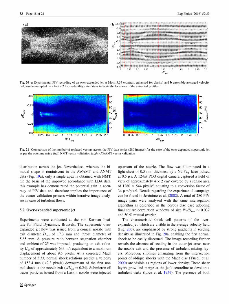
Experiments were conducted at the von Karman Insti-tute for Fluid Dynamics, Brussels. The supersonic over-expanded jet flow was issued from a conical nozzle with exit diameter Dnoz of 17.3 mm and throat diameter of 5.85 mm. A pressure ratio between stagnation chamber and ambient of 25 was imposed, producing an exit veloc-ity Ujet of approximately 633 m/s equivalent to a maximum displacement of about 9.5 pixels. At a corrected Mach number of 3.33, normal shock relations predict a velocity of 153.4 m/s (≈2.3 pixels) downstream of the first nor-mal shock at the nozzle exit (u/Ujet ≈ 0.24). Submicron oil tracer particles issued from a Laskin nozzle were injected

upstream of the nozzle. The flow was illuminated in a light sheet of 0.5 mm thickness by a Nd:Yag laser pulsed at 0.5 μs. A 12-bit PCO digital camera captured a field of view of approximately 4 × 2 cm2 covered by a sensor area of 1280 × 544 pixels2, equating to a conversion factor of 34 μm/pixel. Details regarding the experimental campaign can be found in Jerónimo et al. (2002). A total of 280 PIV image pairs were analysed with the same interrogation algorithm as described in the porous disc case adopting final square correlation windows of size WS/Dnoz ≈ 0.037 and 50 % mutual overlap.

The characteristic shock cell patterns of the over-expanded jet, which are visible in the average velocity field (Fig. 20b), are emphasised by strong gradients in seeding density as illustrated in Fig. 20a, enabling the first normal shock to be easily discerned. The image recording further reveals the absence of seeding in the outer jet areas near the nozzle exit and the presence of turbulent mixing lay-ers. Moreover, sliplines emanating from the intersection points of oblique shocks with the Mach disc (Yüceil et al. 2000) are visible as regions of lower density. These shear layers grow and merge at the jet’s centreline to develop a turbulent wake (Love et al. 1959). The presence of both

Fig. 20 a Experimental PIV recording of an over-expanded jet at Mach 3.33 (contrast enhanced for clarity) and b ensemble-averaged velocity field (under-sampled by a factor 2 for readability). Red lines indicate the locations of the extracted profiles

Fig. 21 Comparison of the number of replaced vectors across the PIV data series (280 images) for the case of the over-expanded supersonic jet as per the outcome using (left) NMT vector validation (right) AWAMT vector validation

Exp Fluids (2016) 57:33

1 3

Page 19 of 21 33

inhomogeneous seeding concentrations and rapid changes in flow scales makes this flow field susceptible to over-detection and constitutes a challenging test case for vector validation.

Comparison of the percentage of replaced vectors R in Fig. 21 reveals the traditional NMT approach to replace a higher number of vectors (~30 %) in the vicinity of the nor-mal shock (x/Dnoz ≈ 0.25) compared to AWAMT (RAW-

AMT ≈ 10 %). This tendency can be observed to continue along the central sliplines. The outer turbulent shear layers are also susceptible to a slightly higher probability of vector replace-ment with NMT due to the velocity gradients. On the other hand, NMT arguably invalidates less vectors in the regions of very low seeding density (x/Dnoz ≤ 0.75, |y/Dnoz| ≈ 0.5) where unreliable correlation can be expected, whereas AWAMT cor-rectly invalidates a higher percentage of vectors.

The detrimental effects of over-detection are again noticeable when juxtaposing profiles of ensemble statistics in horizontal velocity magnitude (Fig. 22) and turbulence intensity (Fig. 23). Near the nozzle (x/Dnoz = 0.1), differ-ences between NMT, ANMT and AWAMT in terms of streamwise velocity are negligible within the potential core of the jet but become apparent in the outer, poorly seeded regions. The outer regions are nevertheless attributed height-ened RMS levels as vectors, even when re-interpolated, remain unreliable in this region (Fig. 23). It should be noted that presented quantitative data in terms of higher order statistics are associated with larger uncertainty due to the

small number of flow fields. This does not, however, endan-ger their potential to evaluate comparative performances of the assessed validation methods. The profile positioned at x/Dnoz = 0.28 is slightly behind the normal shock. Jerónimo et al. (2002) estimated the amplitude of the normal shock’s average longitudinal oscillation Δx caused by the interaction between the turbulent boundary layer and oblique shocks to be in the order of 1 mm (Δx/Dnoz ~ 0.06). In this area, NMT replaces about 30 % of the vectors. Given the nomi-nal stepwise variation in velocity across the shock, replaced velocities will thus tend towards either higher or lower val-ues. This is evidenced by the corresponding probability den-sity functions (Fig. 23b). The bi-modal probability density function (pdf) relevant to NMT shows elevated probabilities at u/Ujet ≈ 0.3 and u/Ujet ≈ 0.6, whereas AWAMT allows more variety in the retrieved velocity data. Although not depicted, the distribution in horizontal velocity obtained with ANMT is nearly identical to AWAMT, explaining the agreement between the two approaches in terms of mean and turbulence statistics. The inherent velocity bias with NMT artificially introduces a higher longitudinal turbulence level which is visible in the turbulence profile at the corre-sponding spatial location (Fig. 23a). At x/Dnoz = 0.48, the

Fig. 22 a Profiles in average horizontal velocity extracted along the vertical directions indicated in Fig. 20b. b Mean streamwise velocity along the jet centreline

Fig. 23 a Profiles in longitudinal turbulence intensity extracted along the vertical directions indicated in Fig. 20b. b Comparison in prob-ability distribution of horizontal velocity at x/Dnoz = 0.28 incorporat-ing NMT and AWAMT vector validation in PIV

Exp Fluids (2016) 57:33

1 3

33 Page 20 of 21

extraction line crosses the turbulent sliplines. Because of the validation utilising coherency heuristics in AWAMT and ANMT, less vectors are incorrectly identified as outliers, minimising any induced smoothening contrary to the lower turbulence levels obtained with NMT (Fig. 22a). This is in line with the findings for the porous disc. The advantage of the alternative validation process is further evidenced in Fig. 23a by the elevated fluctuation levels in the outer shear layers, which at this downstream position start to become properly seeded. More importantly, NMT hinders accurate retrieval of the evolution in centreline velocity across the shock. Figure 22b reveals choosing a more conducive vec-tor validation process is capable of reducing the associated modulation in velocity jump; u/Ujet = 0.38 with NMT and u/Ujet = 0.37 with AWAMT versus the theoretical value of u/Ujet = 0.24. A difference between AWAMT and ANMT is also noticeable with the latter yielding a u/Ujet = 0.375. The figure also shows that by incorrectly replacing more vectors along the turbulent slipline (cf. Fig. 21), and NMT predicts a faster velocity recovery. Further downstream differences between the validation methods become negligible in terms of vector replacement equating their performances relevant to velocity statistics.

6 Conclusions

Velocity fields obtained from PIV image analysis tech-niques are always contaminated with erroneous vectors, and such outliers often appear in clusters as a result of underlying degraded image quality or strong gradients in flow velocity. Existing validation methodologies for instan-taneous PIV velocity fields are commonly based on com-parison of the scrutinised vector with its immediate neigh-bourhood. As a result, such methods are unable to detect false vectors when clustered and are moreover prone to mistakenly invalidate correct vectors. For this reason, a novel adaptive method for outlier detection has been pro-posed in this paper with the aim to render validation pro-cesses more robust in the presence of outlier clusters. The detection of false vectors will thereby be improved and over-detection can be reduced without the need to fine-tune inherent parameters.

The proposed method emulates the process of outlier detection in human vision whereby the considered neigh-bourhood for comparison is a priori extended until the data-base is sufficiently reliable for posterior validation tasks. Selection of the appropriate vicinity is dictated by a meas-ure of coherency. The latter is quantified as the discrep-ancy between local velocity values and a parabolic regres-sion. For each vector, the neighbourhood is automatically enlarged until at least half the enclosed vectors are coher-ent. To further improve the validation algorithm, vector

comparison is performed on the basis of magnitude and direction instead of the traditional horizontal and vertical vector components. To limit the potential diversity in vec-tor direction, the acceptable background fluctuation level is automatically adjusted to the vector magnitude and consti-tutes a second feature of adaptivity. Moreover, applicability to both structured and unstructured data grids is ensured by the implementation of a distance-based Gaussian weighting system.

The algorithm has been assessed with Monte Carlo simulations using three flow fields: an isolated vortex, a turbulent channel flow and a DNS simulation of isotropic turbulence. Flow fields were contaminated with outliers of varying magnitude and degree of clustering. The common outlier detection schemes resulted in high numbers of unde-tected outliers and number of wrongly invalidated correct vectors. Depending on the amount of clustering and outlier magnitude as much as 80 % of the spurious vectors could remain undetected, while 3 % of the total vectors could be over-detected. Implementation of the coherency adaptiv-ity dramatically improved the outlier detection, potentially reducing the under-detection by as much as one-fourth for small outlier magnitudes or even one-tenth for larger mag-nitudes. These findings advocate coherency adaptivity to be a powerful tool to improve the performance of existing validation routines even in the presence of outlier clusters. The concept is computationally simple and implementation is straightforward, even in established validation routines. Validation on the basis of angle and magnitude enabled a further lowering of the missed outliers and mistaken out-liers especially in case of lower displacement magnitudes. Overall, the proposed validation method proved to be the most robust and general without any reliance on user-defined parameters. Related validation performances con-sistently surpassed the traditional routines and were better or at least on a par with the adaptivity enhanced conven-tional methodologies.

When implemented in a standard PIV image analy-sis process and applied to experimental PIV images of a porous disc’s near-wake and over-expanded supersonic jet, the proposed outlier detection routine was shown to be capable of identifying more erroneous vectors (improved under-detection). As a consequence of the adaptive vali-dation in terms of velocity magnitude and direction, over-detection was simultaneously reduced in turbulent flow regions. When incorporating the presented valida-tion method, PIV data were in better agreement with LDA measurements and theoretical analyses, proving its ability to ameliorate the measurement accuracy and resolution.

Acknowledgments This work has been funded by the UK’s Engi-neering and Physical Sciences Research Council (EPSRC - EP/L010755/1). The authors greatly appreciate their support.

Exp Fluids (2016) 57:33

1 3

Page 21 of 21 33

Open Access This article is distributed under the terms of the Creative Commons Attribution 4.0 International License (http://crea-tivecommons.org/licenses/by/4.0/), which permits unrestricted use, distribution, and reproduction in any medium, provided you give appropriate credit to the original author(s) and the source, provide a link to the Creative Commons license, and indicate if changes were made.

References

Aguí JC, Jiménez J (1987) On the performance of particle tracking. J Fluid Mech 185:447–468

Anderson E, Spall R (2001) Experimental and numerical investigation of two-dimensional parallel jets. J Fluids Eng 123:401–406

Astarita T, Cardone G (2005) Analysis of interpolation schemes for image deformation methods in PIV. Exp Fluids 38:233–243

Duncan J, Dabiri D, Hove J, Gharib M (2010) Universal outlier detec-tion for particle image velocimetry (PIV) and particle tracking velocimetry (PTV) data. Meas Sci Technol 21:057002

Etabari A, Vlachos PP (2005) Improvements on the accuracy of deriv-ative estimation from DPIV velocity measurements. Exp Fluids 39:1040–1050

Garcia D (2011) A fast all-in-one method for automated post-process-ing of PIV data. Exp Fluids 50:1247–1259

Gould RD, Loseke WK (1993) A comparison of four velocity bias correction techniques in Laser Doppler Velocimetry. J Fluids Eng 115(3):508–514

Griffin J, Schultz T, Holman R, Ukeiley L, Cattafesta L (2010) Appli-cation of multi-variate outlier detection to fluid velocity meas-urements. Exp Fluids 49:305–317

Hunt JCR, Wray AA, Moin P (1988) Eddies, streams, and conver-gence zones in turbulent flows. In: Proceedings of the summer program 1988, Center for Turbulence Research

Jerónimo A, Riethmuller ML, Chazot O (2002) PIV application to Mach 3.75 overexpanded jet. In: Proceedings 11th international symposium on application of laser techniques to fluid mechan-ics, Lisbon, Portugal

Kalra TR, Uhlherr PHT (1971) Properties of bluff body wakes. In: 4th Australasian conference on hydraulics and fluid mechanics, Melbourne, Australia

Keane RD, Adrian RJ (1992) Theory of cross-correlation analysis of PIV images. Appl Sci Res 49:191–215

Lecuona A, Nogueira J, Rodríguez PA (2002) Data validation, interpolation and signal to noise increase in iterative PIV methods. In: Proceedings of the 11th international symposium on applications of laser techniques to fluid mechanics, Lisbon, Portugal

Li Y, Perlman E, Wan M, Yang Y, Burns R, Meneveau C, Burns R, Chen S, Szalay A, Eyink G (2008) A public turbulence database cluster and applications to study Lagrangian evolution of veloc-ity increments in turbulence. J Turbul 9:31

Liang DF, Jiang CB, Li YL (2003) Cellular neural network to detect spurious vectors in PIV data Exp. Fluids 34:52–62

Lin YF, Sheu MJ (1990) Investigation of two parallel unventilated jets. Exp Fluids 10:17–22

Love ES, Grigsby CE, Lee LP, Woodling MJ (1959) Experimental and theoretical studies of axisymmetric free jets. NASA Techni-cal report R-6

Miau JJ, Leu TS, Liu TW, Chou JH (1997) On vortex shedding behind a circular disk. Exp Fluids 23:225–233

Nogueira J, Lecuona A, Rodríguez PA (1997) Data validation, false vectors correction and derived magnitudes calculation on PIV data. Meas Sci Technol 8:1493–1501

Raben SG, Charonko JJ, Vlachos PP (2012) Adaptive gappy proper orthogonal decomposition for particle image velocimetry data reconstruction. Meas Sci Technol 23:025303

Raffel M, Leitl B, Kompenhans J (1992) Data validation for particle image velocimetry. In: Proceedings of the 6th international sym-posium on application of laser techniques to fluid mechanics. Lisbon, Portugal

Raiola M, Discetti S, Ianiro A (2015) On PIV random error minimi-zation with optimal POD-based low-order reconstruction. Exp Fluids 56:75

Reiz B, Pongor S (2011) Psychologically inspired, rule-based outlier detection in noisy data. In: Proceedings 13th international sym-posium on symbolic and numeric algorithms for scientific com-puting, Timisoara, Romania

Scarano F (2004) A super-resolution particle image velocimetry inter-rogation approach by means of velocity second derivatives cor-relation. Meas Sci Technol 15:475

Scarano F, Riethmuller ML (2000) Advances in iterative multigrid PIV image processing. Exp Fluids 29:S51–S60

Sciacchitano A, Dwight RP, Scarano F (2012) Navier-stokes simula-tions in gappy PIV data. Exp Fluids 53(5):1421–1435

Shinneeb A-M, Bugg JD, Balachandar R (2004) Variable thresh-old outlier identification in PIV data. Meas Sci Technol 15:1722–1732

Song X, Yamamoto F, Iguchi M, Murai Y (1999) A new tracking algo-rithm of PIV and removal of spurious vectors using Delaunay tessellation. Exp Fluids 26:371–380

Stanislas M, Okamoto K, Kaehler CJ (2001) Main results of the first international PIV challenge. Meas Sci Technol 14:R63–R89

Stanislas M, Okamoto K, Kaehler CJ, Westerweel J (2003) Main results of the second international PIV challenge. Exp Fluids 39:170–191

Tanaka E (1970) The interference of two dimensional parallel jets: 1st report, experiments on a dual jet. Bull JSME 13(56):272–280

Theunissen R, Scarano F, Riethmuller ML (2007) An adaptive sam-pling and windowing interrogation method in PIV. Meas Sci Technol 18:275–287

Wang H, Gao Q, Feng L, Wei R, Wang J (2015) Proper orthogonal decomposition based outlier correction for PIV data. Exp Fluids 56:43

Westerweel J (1994) Efficient detection of spurious vectors in particle image velocimetry data. Exp Fluids 16:236–247

Westerweel J (2008) On velocity gradients in PIV interrogation. Exp Fluids 44:831–842

Westerweel J, Scarano F (2005) Universal outlier detection for PIV data. Exp Fluids 39:1096–1100

Young CN, Johnson DA, Weckman EJ (2004) A model-based valida-tion framework for PIV and PTV. Exp Fluids 36:23–25

Yüceil KB, Ötügen MG, Arik E (2000) Underexpanded sonic jets: a PIV study. In: 10th international symposium on application of laser techniques to fluid mechanics, Lisbon, Portugal