Takustraße 7D-14195 Berlin-Dahlem

GermanyKonrad-Zuse-Zentrumfur Informationstechnik Berlin

CORINNA KLAPPROTH, ANTON SCHIELA, ANDPETER DEUFLHARD

Adaptive Timestep Control for theContact–Stabilized Newmark Method1

1Supported by the DFG Research Center Matheon, “Mathematics for key technologies: Mod-elling, simulation, and optimization of real-world processes”, Berlin

ZIB-Report 10-09 (June 2010)

Adaptive Timestep Control for the Contact–Stabilized

Newmark Method†

Corinna Klapproth, Anton Schiela, and Peter Deuflhard

June 25, 2010

Abstract

The aim of this paper is to devise an adaptive timestep control in thecontact–stabilized Newmark method (ContacX) for dynamical contact prob-lems between two viscoelastic bodies in the framework of Signorini’s condition.In order to construct a comparative scheme of higher order accuracy, we ex-tend extrapolation techniques. This approach demands a subtle theoreticalinvestigation of an asymptotic error expansion of the contact–stabilized New-mark scheme. On the basis of theoretical insight and numerical observations,we suggest an error estimator and a timestep selection which also cover thepresence of contact. Finally, we give a numerical example.

AMS MSC 2010: 35L86, 74M15, 65K15, 65L06

Keywords: dynamical contact problems, contact–stabilized Newmark method, ex-trapolation methods, adaptivity, timestep control

1 Introduction

Dynamical contact problems arise in different applications such as biomechanics. Inclassical approaches, they are modelled via Signorini’s contact conditions which arebased on the non-penetration of mass. Both in analytical models and in numericalschemes, the resulting nonsmooth and nonlinear variational inequalities give rise tofundamental mathematical difficulties.

Concerning the time discretization of dynamical contact problems, the Newmarkmethod is one of the most popular numerical integrators. As it is well-known, theclassical scheme may lead to artificial numerical oscillations at dynamical contactboundaries, and even an undesirable energy blow-up during time integration mayoccur [6, 19]. In [13], Kane, Repetto, Ortiz, and Marsden introduced an improved

†Supported by the DFG Research Center Matheon, “Mathematics for key technologies: Mod-elling, simulation, and optimization of real-world processes”, Berlin

1

2

variant of Newmark’s method which is energy dissipative at contact, but still unableto avoid the oscillations at contact boundaries. For this reason, Deuflhard, Krause,and Ertel suggested a contact–stabilized Newmark method [6, 19] which avoids theunphysical oscillations and is still energy dissipative at contact. This is the timeintegration scheme of interest in the present paper.

In view of challenging real life problems (e.g., the motion of a human knee,see [19]), an adaptive control of timestep is of crucial importance in order to increasethe efficiency of the contact–stabilized Newmark method (called CSN further on).A mesh of equidistant timesteps can not be expected to be adequate for reaching agiven accuracy of the approximation of a reasonable computational effort.

The construction of an adaptive timestep control requires a realistic estimationof the consistency error (cf., e.g., the textbook [5]). As a necessary preparatory step,we studied the stability of dynamical contact problems under perturbation of theinitial data [16]. For viscoelastic materials, we found a characterization of a classof problems for which a perturbation result can be expected even in the presenceof contact. This gave us the idea about a specific norm in function space whichhas been exploited for the estimation of the consistency error of Newmark meth-ods. In the unconstrained situation, the symmetric Newmark scheme is equivalentto the Stormer-Verlet scheme which is well–known to be second order consistent(see, e.g., [12]). In the constrained situation, we have proven an estimate for theconsistency error of the classical Newmark method, the modified Newmark methodby Kane et al., and the contact–stabilized Newmark method under the assumptionof bounded total variation of the solution [17].

The paper is organized as follows. We will start with a short exposition of thedynamical Signorini contact problem and the contact–stabilized Newmark methodin Section 2. Further, we will sum up known consistency and sensitivity resultsfor the scheme. In Section 3, we will analyze the existence of an asymptotic errorexpansion of the discretization error theoretically as well as numerically. Theseresults are the basis for the application of modified extrapolation methods in orderto construct a comparative scheme of higher order. Finally, in Section 4, we willsuggest a problem-adapted error estimator and a suitable timestep selection (calledContacX). We will conclude the paper by a numerical example in Section 5.

2 Notation and Background

In order to fix notation, we write down the classical contact problem formulationfor linearly viscoelastic materials via Signorini’s contact conditions. Afterwards,we present the corresponding contact–stabilized Newmark method, and we reviewexisting sensitivity and consistency results for the scheme.

2.1 Problem formulation

Our model for dynamical contact between two bodies is based on linearized Sig-norini’s contact conditions. In view of existing perturbation and consistency results,

3

see [16] and [17], we consider linear viscoelastic bodies fulfilling the Kelvin-Voigtconstitutive law. For the convenience of the reader, here we merely collect thenotation used therein.

Notation. Let the two bodies be identified with the union of two domains whichare understood to be bounded subsets in Rd with d = 2, 3. Each of the bound-aries are assumed to be Lipschitz and decomposed into three disjoint parts: ΓD,the Dirichlet boundary, ΓN , the Neumann boundary, and ΓC , the possible contactboundary. The actual contact boundary is not known in advance, but is assumed tobe contained in a compact strict subset of ΓC . The Dirichlet boundary conditionsgive rise to H1

D := v |v ∈ H1, v|ΓD= 0.

Tensor and vector quantities are written in bold characters, e.g., v. Time deriva-tives are indicated by dots ( ˙ ). For the sake of clear arrangement, we use theabbreviation v = (v, v) for a function and its first time derivative.

For given Banach space V and time interval t0 < T < ∞, let C([t0, T ],V)be the continuous functions v : [t0, T ] → V. The space L2(t0, T ;V) consists of allmeasurable functions v : (t0, T ) → V for which ‖v‖2

L2(t0,T ;V) :=∫ Tt0‖v(t)‖2

V dt < ∞holds. We identify L2 with its dual space and obtain the evolution triple H1 ⊂L2 ⊂ (H1)∗ where we denote the dual space to H1 by (H1)∗. With reference tothis evolution triple, the Sobolev space W1,2(t0, T ;H1,L2) means the set of allfunctions v ∈ L2(t0, T ;H1) that have generalized derivatives v ∈ L2(t0, T ; (H1)∗),see, e.g., [24].

We will need the (total) variation TV(v, [t0, T ],V) of a function v : [t0, T ] → V.The set of all functions from [t0, T ] into V that have bounded variation is denotedby BV([t0, T ],V), compare, e.g., [22].

Non-penetration condition. At the contact interface ΓC , the two bodies maycome into contact but must not penetrate each other. We assume a bijective map-ping φ : ΓS

C −→ ΓMC between the two possible contact surfaces to be given. Follow-

ing [8], we define linearized non-penetration with respect to φ by

[u · ν]φ(x, t) = uS(x, t) · νφ(x) − uM (φ(x), t) · νφ(x) ≤ g(x) , x ∈ ΓSC .

This condition is given with respect to the initial gap

ΓSC 3 x 7→ g(x) = |x − φ(x)| ∈ R

between the two bodies in the reference configuration, and we have set

νφ =

φ(x) − x

|φ(x) − x|, if x 6= φ(x) ,

µS(x) = −µM (x) , if x = φ(x) .

4

Variational problem formulation. For the weak formulation of the dynamicalcontact problem, the convex set of all admissible displacements is denoted by

K = v ∈ H1D | [v · ν]φ ≤ g . (1)

The materials under consideration are assumed to be linearly viscoelastic, i.e.the stresses satisfy the Kelvin-Voigt constitutive relation. Both elasticity and vis-coelasticity tensors should be sufficiently smooth, symmetric, and uniformly positivedefinite.

The external forces are represented by a linear functional fext on H1D which

accounts for the volume forces and the tractions on the Neumann boundary. Theinternal forces can be written as a bilinear form a in H1 for the linearly elastic part,respectively b for the viscous part. Both bilinear forms are bounded in H1 and giverise to seminorms ‖ · ‖2

a = a(·, ·) and ‖ · ‖2b = b(·, ·). The sum of internal elastic and

external forces can be represented by

〈F(w),v〉(H1)∗×H1 = a(w,v) − fext(v) , v,w ∈ H1 ,

and the viscoelastic forces can be written as

〈G(w),v〉(H1)∗×H1 = b(w,v) , v,w ∈ H1 .

Via integration by parts and exploiting the boundary conditions, see [7] and [14],the contact problem in the weak formulation can be written as a variational in-equality: For almost every t ∈ [0, T ], find u ∈ K with u(·, t) ∈ C([0, T ],H1) andu ∈ W1,2(0, T ;H1,L2) such that for all v ∈ K

〈u,v − u〉(H1)∗×H1 + 〈F(u),v − u〉(H1)∗×H1 + 〈G(u),v − u〉(H1)∗×H1 ≥ 0 (2)

andu(0) = u0 , u(0) = u0 . (3)

Incorporating the constraints v(t) ∈ K for almost every t ∈ [0, T ] by the character-istic functional IK(v), the variational inequality (2) can equivalently be formulatedas the variational inclusion

0 ∈ u + F(u) + G(u) + ∂IK(u)

utilizing the subdifferential ∂IK of IK (see, e.g., [9]). For a given solution u of thisvariational inequality and for almost every t ∈ [0, T ], we define the contact forcesFcon(u) ∈ (H1)∗ by

〈Fcon(u),v〉(H1)∗×H1 = 〈u + F(u) + G(u),v〉(H1)∗×H1 , v ∈ H1 . (4)

As shown for instance in [1], the unilateral contact problem between a viscoelasticbody and a rigid foundation has at least one weak solution. In the following, werepresent the state of a solution u of (2) for tn, tn+1 ∈ [0, T ] by

u(tn+1) = Φtn+1,tn(u(tn), u(tn)) , u(tn+1) = Φtn+1,tn(u(tn), u(tn))

with the evolution operator Φtn+1,tn := (Φtn+1,tn , Φtn+1,tn) : H1 × L2 −→ H1 × L2.

5

2.2 Contact–stabilized Newmark scheme

Here, we turn towards the spatiotemporal discretization of the dynamical contactproblem (2). We use the method of time layers (MOT), also known as Rothemethod, in which we discretize first in time and then in space.

For integration in time, we consider the contact–stabilized Newmark method(CSN) as suggested by Deuflhard, Krause, and Ertel for the purely elastic case [6].This scheme is energy dissipative in the presence of contact and avoids the occur-rence of artificial numerical oscillations at contact boundaries. The latter featureis achieved by performing a discrete L2-projection at contact interfaces at eachtimestep. In [17], the authors have given the generalization of the contact–stabilizedNewmark method to the viscoelastic case.

In order to fix notation, let the continuous time interval [t0, T ] be subdividedby N∆τ + 1 discrete time points t0 < t1 < · · · < tN∆τ

= T which are forming anequidistant mesh ∆τ = t0, t1, . . . , T. The constant timestep is denoted by τ .

Contact–stabilized Newmark method (CSN).

0 ∈ un+1pred −

(un + τ un

)+ ∂IK

(un+1

pred

)0 ∈ un+1 − un+1

pred +12τ2

(F

(un+un+1

2

)+ G

(un+1−un

τ

)+ ∂IK

(un+1

))un+1 = un − τ

(F

(un+un+1

2

)+ G

(un+1−un

τ

)− Fcon

(un+1

)) (5)

where the contact forces Fcon

(un+1

)are defined by

12τ2

⟨Fcon

(un+1

),v

⟩(H1)∗×H1 (6)

=⟨un+1 − un+1

pred +12τ2

(F

(un+un+1

2

)+ G

(un+1−un

τ

)),v

⟩(H1)∗×H1

, v ∈ H1 .

We assume that the spatial quantities corresponding to un are obtained via finiteelements Sh with a spatial mesh size parameter h > 0. In this setting, K ⊂ Sh has tobe understood as a discrete approximation of the set of admissible displacements.For details concerning the spatial discretization, we refer the reader to [14, 18].The arising constrained minimization problems in space can be solved by adaptivemonotone multigrid methods (see [10, 18, 19]).

In analogy to the continuous problem, we define the discrete evolution operatorΨtn+1,tn :=

(Ψtn+1,tn , Ψtn+1,tn

): H1 × L2 −→ H1 × L2 for tn, tn+1 ∈ ∆τ via

un+1 = Ψtn+1,tn(un, un

), un+1 = Ψtn+1,tn

(un, un

).

Moreover, we introduce the lattice function uτ :=(uτ , uτ

): ∆τ −→ H1 × L2 as

uτ (tn+1) = Ψtn+1,tn(uτ (tn), uτ (tn)

), uτ (tn+1) = Ψtn+1,tn

(uτ (tn), uτ (tn)

)with

uτ (t0) = u0 , uτ (t0) = u0 .

6

Remark 2.1. In [17], the authors have proven that the contact–stabilized Newmarkmethod coincides with the modified Newmark scheme by Kane et al. ([13]) infunction space. Since we use the method of time layers, the numerical analysis inthis paper will cover both Newmark methods simultaneously. Nevertheless, we willrestrict our considerations to CSN due to its nice numerical features.

2.3 Sensitivity and consistency results

In Section 3, we will work out an asymptotic error expansion of the contact–stabilized Newmark method. For the convenience of the reader, we recall knownresults concerning the sensitivity and consistency of the scheme from [17] and [21].

Conical derivative. First of all, we need the well–posedness of CSN with respectto perturbations of the initial data. In [21], an important result has been given whichconcerns the directional differentiability of the solution u = u(f) ∈ K of an ellipticvariational inequality

a(u,v − u) ≥ 〈f ,v − u〉V∗×V , ∀ v ∈ K

on a Hilbert space V. The convex set K is of the form K = w ∈ V | w ≤ g a.e.with g continuous, a(·, ·) has to fulfill usual ellipticity and continuity assumptions,and f ∈ V∗. Then, the mapping f −→ u(f) has a conical derivative Du(f)(·) onV∗, and Du(f)(w) ∈ Ku is the solution of the variational inequality

a(Du(f)(w),v − Du(f)(w)) ≥ 〈w,v − Du(f)(w)〉V∗×V , ∀ v ∈ Ku

with a modified admissible set

Ku = w ∈ V |w ≤ 0 if u = g, a(u,w) = 〈f ,w〉V∗×V .

The transfer of this result to CSN yields the following sensitivity result.

Theorem 2.2 ([21]). The discrete evolution operator(Ψt+τ,t, Ψt+τ,t

)possesses a

conical derivative DΨt+τ,t :=(DΨt+τ,t, DΨt+τ,t

), i.e.

Ψt+τ,t(u + hw) = Ψt+τ,tu + hDΨt+τ,tu(w) + θ(h, w)

and

Ψt+τ,t(u + hw) = Ψt+τ,tu + hDΨt+τ,tu(w) +2τθ(h, w)

where

limh→0

‖θ(h, w)‖H1/h = 0

7

for all h > 0 and u = (u, u) , w = (w, w) ∈ H1 × L2. The conical derivative isgiven as the solution of

0 ∈ wpred − (w + τw) + ∂IKΨt+τ,tu

(wpred

)0 ∈ DΨt+τ,tu(w) − wpred +

12τ2

(F

(w+DΨt+τ,tu(w)

2

)+ G

(DΨt+τ,tu(w)−w

τ

)+ ∂IKΨt+τ,tu

(DΨt+τ,tv(w)

))DΨt+τ,tu(w) = w − τ

(F

(w+DΨt+τ,tu(w)

2

)+ G

(DΨt+τ,tu(w)−w

τ

)−Fcon

(DΨt+τ,tu(w)

))(7)

with contact forces

12τ2

⟨Fcon

(DΨt+τ,tu(w)

),v

⟩(8)

=⟨DΨt+τ,tu(w) − wpred +

12τ2

(F

(w+DΨt+τ,tu(w)

2

)+ G

(DΨt+τ,tu(w)−w

τ

)),v

⟩for v ∈ H1 and

KΨt+τ,tu =w ∈ H1

D

∣∣ [w ·ν]φ ≤ 0 if[Ψt+τ,tu ·ν

]φ

= g,⟨Fcon

(Ψt+τ,tu

),w

⟩= 0

.

(9)

The conical derivative is defined via CSN on a modified admissible set KΨt+τ,tu.Strict complementarity implies that [DΨt+τ,tu(w) · ν]φ = 0 on those parts of thepossible contact boundaries where [Ψt+τ,tu·ν]φ = g. Then, the variational inclusionin the second line of the scheme reduces to a minimization problem with time-dependent Dirichlet boundaries. The theorem does not give any information aboutthe sensitivity of CSN in the special case of interest where h coincides with theparameter τ .

Remark. A simple calculation shows that

DΨt+τ,tu(w) = w +2τ

(DΨt+τ,tu(w) − wpred

).

In [17], the authors have proven that the predictor wpred resulting from a L2-projection converges to w + τw if the spatial discretization parameter h tends tozero. Hence, we find the relation

DΨt+τ,tu(w) = −w +2τ

(DΨt+τ,tu(w) − w

)(10)

in function space.

8

Physical energy norm. In [16], the authors introduced a mix of norms in func-tion space which allows to prove a perturbation result for a class of dynamicalcontact problems of type (2). For a function v = (v, v) : [t, t + τ ] → H1 × L2 withv ∈ L2(t, t + τ,H1), we define

‖v‖2E(t,τ) := ‖v(t + τ)‖2

E +

t+τ∫t

∥∥v(s)∥∥2

bds (11)

in terms of‖v(t + τ)‖2

E :=12

∥∥v(t + τ)∥∥2

L2 +12

∥∥v(t + τ)∥∥2

a. (12)

The physical energy norm may be interpreted as the sum of the kinetic energy, thepotential energy, and the viscoelastic part.

Consistency error. In [17], the authors derived an estimate for the consistencyerror of the classical Newmark method, the modified Newmark method by Kane etal., and CSN within the physical energy norm∥∥Ψ − Φ

∥∥2

E(t,τ):=

12

∥∥Ψt+τ,tu(t) − Φt+τ,tu(t)∥∥2

L2 +12

∥∥Ψt+τ,tu(t) − Φt+τ,tu(t)∥∥2

a

+

t+τ∫t

∥∥∥Ψt+s,tu(t) − u(t)τ

− Φt+s,tu(t)∥∥∥2

bds .

In the presence of contact, this result requires the solution of the dynamical contactproblem together with its first and second derivative to be in the function space ofbounded variation.

Theorem 2.3 ([17]). Let u ∈ BV([t, t + τ ],H1

)and u ∈ BV

([t, t + τ ], (H1)∗

).

Then, for initial values un = u(t) and un = u(t), the consistency error of CSN interms of Ψ = (Ψ, Ψ) satisfies∥∥Ψ − Φ

∥∥E(t,τ)

= R(u, [t, t + τ ]) · O(τ1/2

)where

R(u, [t, t + τ ]) := TV(u, [t, t + τ ],H1

)+ TV

(u, [t, t + τ ],H1

)+ TV

(u, [t, t + τ ], (H1)∗

). (13)

The formulation of the consistency result in function space does not give anyinformation about the spatial distribution of the consistency error of CSN. Analyz-ing the proof of the theorem as presented in [17], we find that the estimate can beimproved if the active contact boundaries do not change during the timestep. Thisresult will be verified in detail in a PhD thesis [15].

A central role for the construction of an adaptive timestep control is played bythe choice of norm in which the approximation error of the scheme is measured.

9

The existing perturbation and consistency results for CSN suggest to use the fullphysical energy norm ‖ · ‖E . In the absence of contact, the Newmark scheme haspointwise the consistency order 2 in positions as well as velocities. Hence, due tothe integral over time, the viscoelastic part of the physical energy norm is of higherorder than the kinetic and potential parts. In view of an adaptive timestep control,we neglect the viscoelastic part, and we are only interested in the reduced physicalenergy norm ‖ · ‖E .

3 Towards an asymptotic error expansion

The main challenge for an adaptive timestep control is the construction of a suitableerror estimator. Usually, the numerical integrator of interest is compared to a sec-ond, higher order discrete evolution. We want to construct such a scheme by meansof extrapolation techniques which are based on an asymptotic error expansion. Thescope of this section is to analyze the existence of such an error representation forthe contact–stabilized Newmark method.

3.1 Extension of extrapolation techniques

For ordinary differential equations, a proof technique for an asymptotic error expan-sion can be found in [11]. Here, we will extend this approach to dynamical contactproblems.

We define a discrete evolution Ψt+τ,t∗ := (Ψt+τ,t

∗ , Ψt+τ,t∗ ) : H1 ×L2 −→ H1 ×L2

via the formulas

Ψt+τ,t∗ u(t) := Ψt+τ,t(u(t) + e(t)τp) − e(t + τ)τp

Ψt+τ,t∗ u(t) := Ψt+τ,t(u(t) + e(t)τp) − ε(t + τ)τp .

(14)

For fixed initial time t0, the functions e := (e, ε) : [t0, T ] → H1 × L2 should haveinitial values equal to zero, i.e.

e(t0) = 0 , ε(t0) = 0 . (15)

We will specify these functions in Section 3.2 below. For constant stepsize τ , thelattice function u∗

τ = (u∗τ , u

∗τ ) : ∆τ −→ H1 × L2 of the new evolution correlates

with the one of CSN in the following way.

Lemma 3.1. For t ∈ ∆τ , the lattice functions (u∗τ , u

∗τ ) and (uτ , uτ ) satisfy the

relation

uτ (t) − u(t) − e(t)τp = u∗τ (t) − u(t)

uτ (t) − u(t) − ε(t)τp = u∗τ (t) − u(t) .

Proof. Due to definition (14) with initial values (15), we find

u∗τ (t0 + τ) = Ψt0+τ,t0(u(t0) + e(t0)τp) − e(t0 + τ)τp = uτ (t0 + τ) − e(t0 + τ)τp .

10

An induction leads to

u∗τ (t) = Ψt,t−τ (u∗

τ (t − τ) + e(t − τ)τp) − e(t)τp = uτ (t) − e(t)τp

which gives the desired relation.

The lemma yields an asymptotic error expansion of order p for CSN if theapproximation error u∗

τ−u of the new scheme is of order o(τp). In order to gain moreinformation on this quantity, we consider the error of the scheme after performingtwo timesteps with stepsize τ/2, for simplicity. The global error of a numericalintegration is based on the continuous dependence of the scheme on the initialdata.

Assumption 3.2. Let CSN fulfill∥∥Ψt+τ,tu(t) − Ψt+τ,t ¯u(t)∥∥

E≤ Cp ·

∥∥u(t) − ¯u(t)∥∥

E

with a constant Cp > 0.

In [16], the validity of the continuous analogon of this perturbation result hasbeen proven for a certain class of dynamical contact problems. The discrete per-turbation behavior will be discussed in a PhD thesis [15]. Now, we can prove anestimate for the approximation error of the new scheme (Ψ∗, Ψ∗).

Theorem 3.3. Let Assumption 3.2 hold. Then,∥∥u∗τ2(t + τ) − u(t + τ)

∥∥E

≤ Cp ·∥∥∥(

Ψt+ τ

2,t

∗ − Φt+ τ2,t)u(t)

∥∥∥E

+∥∥∥(

Ψt+τ,t+ τ

2∗ − Φt+τ,t+ τ

2

)u(t +

τ

2

)∥∥∥E

.

Proof. The error of a numerical scheme after performing two timesteps can bedivided into the consistency error of the second step and the propagation of theconsistency error of the first step, i.e.

u∗τ2(t + τ) − u(t + τ)

= Ψt+τ,t+ τ

2∗ Ψ

t+ τ2,t

∗ u(t) − Φt+τ,t+ τ2 Φt+ τ

2,tu(t)

= Ψt+τ,t+ τ

2∗ Ψ

t+ τ2,t

∗ u(t) − Ψt+τ,t+ τ

2∗ Φt+ τ

2,tu(t) +

(Ψ

t+τ,t+ τ2

∗ − Φt+τ,t+ τ2

)u(t +

τ

2

).

Due to definitions (14)–(15) and Assumption 3.2, we find for the propagated con-sistency error∥∥∥Ψt+τ,t+ τ

2∗ Ψ

t+ τ2,t

∗ u(t) − Ψt+τ,t+ τ

2∗ Φt+ τ

2,tu(t)

∥∥∥E

=∥∥∥Ψt+τ,t+ τ

2 Ψt+ τ2,tu(t) − Ψt+τ,t+ τ

2

(Φt+ τ

2,tu(t) + e

(t +

τ

2

)(τ

2

)p)∥∥∥E

≤ Cp ·∥∥∥Ψt+ τ

2,tu(t) −

(Φt+ τ

2,tu(t) + e

(t +

τ

2

)(τ

2

)p)∥∥∥E

= Cp ·∥∥∥(

Ψt+ τ

2,t

∗ − Φt+ τ2,t)u(t)

∥∥∥E

.

This gives the estimate of the theorem.

11

In view of an asymptotic error expansion of CSN, we combine the results ofLemma 3.1 and Theorem 3.3. This yields that we have to construct the functions(e, ε) such that ∥∥Ψt+τ,t

∗ − Φt+τ,t∥∥

E∥∥Ψt+τ,t − Φt+τ,t∥∥

E

→ 0 for τ → 0 , (16)

i.e. the consistency error of (Ψ∗, Ψ∗) in energy norm should be of higher order thanthe one of CSN for arbitrary initial times.

3.2 Construction of a higher order scheme

The task of this section is to find a definition for the functions (e, ε) such that theinitial values (15) and condition (16) on the consistency error of the new scheme arefulfilled. For this purpose, we need information about the pointwise error behaviorof CSN. While such information is given in the absence of contact, up to now, theonly consistency result for CSN in the presence of contact is given in energy norm(cf. Theorem 2.3). Hence, we lay the following analysis of an asymptotic errorexpansion of CSN on a very general basis.

Assumption 3.4. Let the consistency error of CSN be of the form

Ψt+τ,tu − Φt+τ,tu = m(t) · τp+1 + r(t, τ) · τp

Ψt+τ,tu − Φt+τ,tu =∫ t+τ

tµ(s) ds · τp + ρ(t, τ) · τp

(17)

with m ∈ C([0, T ],H1) and m, µ ∈ W1,2(0, T ;H1,L2).

In the following, we will often use the abbreviation m := (m, µ). Please notethat the second line of Assumption 3.4 is not the derivative of the first one due to thedefinition of the discrete evolution operator. The integral term in the consistencyerror of the velocities is related to the viscoelastic part of the physical energy norm.In the classical approach, we would expect a pointwise Taylor expansion of theconsistency error of the scheme. This is included in our ansatz if∫ t+τ

tµ(s) ds = µ(t) · τ + o(τ)

and|r(t, τ)| = o(τ) , |ρ(t, τ)| = o(τ) .

For a perturbation of the initial values of CSN, we write

Ψt+τ,t(u + eτp) − Ψt+τ,tu =(DΨt+τ,tu(e) + p(t, τ)

)· τp

Ψt+τ,t(u + eτp) − Ψt+τ,tu =(DΨt+τ,tu(e) + π(t, τ)

)· τp

(18)

where (DΨt+τ,tu(e), DΨt+τ,tu(e)) denotes the conical derivative of the scheme in-troduced in Section 2.3. A short calculation shows that π(t, τ) = 2

τ p(t, τ), and

12

we will often use the notation p := (p, π). We expect that p(t, τ) and π(t, τ) areof order o(τ). In the case of time-constant Dirichlet boundaries, the variationalproblem is linear and |p(t, τ)| = 0.

On the basis of these notations, we present a formula for the consistency errorof the new evolution (Ψ∗, Ψ∗).

Lemma 3.5. Let Assumption 3.4 hold. Then, the consistency error in terms of thediscrete evolution Ψ∗ = (Ψ∗, Ψ∗) satisfies

Ψt+τ,t∗ u(t) − Φt+τ,tu(t) =

(DΨt+τ,tu(t)(e(t)) − e(t + τ) + τm(t)

)· τp

+ (r(t, τ) + p(t, τ)) · τp

Ψt+τ,t∗ u(t) − Φt+τ,tu(t) =

(DΨt+τ,tu(t)(e(t)) − ε(t + τ) +

∫ t+τ

tµ(s) ds

)· τp

+ (ρ(t, τ) + π(t, τ)) · τp .

Proof. Inserting definition (14) into the consistency error yields

Ψt+τ,t∗ u(t) − Φt+τ,tu(t) = Ψt+τ,t(u(t) + e(t)τp) − e(t + τ)τp − Φt+τ,tu(t) .

Due to Assumption 3.4 on the consistency error of CSN, we find

Ψt+τ,t∗ u(t) − Φt+τ,tu(t) = Ψt+τ,t(u(t) + e(t)τp) − Ψt+τ,tu(t) − e(t + τ) · τp

+ m(t) · τp+1 + r(t, τ) · τp .

Using (18), we end up with

Ψt+τ,t∗ u(t) − Φt+τ,tu(t) =

(DΨt+τ,tu(t)(e(t)) − e(t + τ) + τm(t)

)· τp

+ (r(t, τ) + p(t, τ)) · τp .

Our aim is to define the functions (e, ε) such that the terms of order p + 1 inthe consistency error of (Ψ∗, Ψ∗) vanish, and the scheme is of higher order o(τp+1).This leads us to the following definition of the functions (e, ε).

Variational problem for (e, ε). For almost every t ∈ [t0, T ], find e(·, t) ∈ Ku(t)

with e ∈ C([t0, T ],H1

)and e ∈ W1,2

(t0, T ;H1,L2

)such that for all v(t) ∈ Ku(t)

〈e − µ − m + F(e) + G(e − m),v − e〉(H1)∗×H1 ≥ 0 (19)

ande(t0) = 0 , e(t0) = m(t0) (20)

where

Ku(t) =w ∈ H1

D

∣∣ [w · ν]φ ≤ 0 if [u(t) · ν]φ = g, 〈Fcon(u(t)),w〉(H1)∗×H1 = 0

.(21)

13

Further, we setε(t) = e(t) − m(t) , ∀ t ∈ [t0, T ] (22)

such that the initial values (15) are fulfilled. The contact forces Fcon(e) ∈ (H1)∗

are given by

〈Fcon(e),v〉(H1)∗×H1 = 〈e−µ−m+F(e)+G(e−m),v〉(H1)∗×H1 , v ∈ H1 . (23)

In the case of strict complementarity, we find a parabolic equality with Dirichletboundaries which are varying in time. These boundaries correspond to the activecontact boundaries of the solution of the original variational inequality (2). Hence,we assume that e and its derivatives are of bounded variation in the same sense.

Assumption 3.6. Let the solution of (19) satisfy

e ∈ BV([t, t + τ ],H1

), e ∈ BV

([t, t + τ ], (H1)∗

).

This leads to an estimate for the consistency error of the new evolution (Ψ∗, Ψ∗).

Lemma 3.7. Let Assumptions 3.4 and 3.6 hold. Then, the consistency error interms of the discrete evolution Ψ∗ = (Ψ∗, Ψ∗) satisfies(∥∥Ψt+τ,t

∗ u(t) − Φt+τ,tu(t) − (r(t, τ) + p(t, τ)) · τp∥∥2

E

+τ

4

∥∥∥DΨt+τ,tu(t)(e(t)) − ε(t + τ) +∫ t+τ

tµ(s) ds

∥∥∥2

b· τ2p

)1/2

≤(1

2

∣∣∣⟨Fcon

(DΨt+τ,tu(t)(e(t))

)− Fcon(e(t)), (24)

DΨt+τ,tu(t)(e(t)) − ε(t + τ) +∫ t+τ

tµ(s) ds

⟩(H1)∗×H1

∣∣∣)1/2· τp+1/2

+ R(e, [t, t + τ ]) · O(τp+1/2

)+ o

(τp+1

)with R(e, [t, t + τ ]) defined in (13).

Remark 3.8. Due to the definition of the modified admissible sets (9) and (21),the first term on the right-hand side of (24) can be written as a linear functional onthe part of the possible contact boundaries where Ψt+τ,tu(t) and u(t) are actuallyin contact. Moreover, DΨt+τ,tu(t)(e(t))−ε(t+τ) is zero on the part of the contactboundaries where the active sets of Ψt+τ,tu(t) and u(t + τ) are unchanged andcoincide with those of u(t). This is the same part of the contact boundaries onwhich we may assume that

∫ t+τt µ(s) ds is zero by its definition as the consistency

error of CSN. Hence, the contact term in the estimate (24) is only effective on asmall part of the possible contact boundaries, namely where the active sets vary intime. For most initial times t, this part tends to a set of measure zero as τ → 0.This effect will also become visible in our numerical examples of Section 3.3 andSection 5.

14

The localization of the contact stresses on the critical part of the possible contactboundaries is rather tedious without yielding further insight. In [16], a similarargumentation has been worked out in detail. Hence, we leave it at this heuristicdiscussion. Instead, we will use a rough estimate for the contact term on the right-hand side of (24) in our main theorem.

Proof. By means of Lemma 3.5, the physical energy norm of the consistency erroris of the form∥∥Ψt+τ,t

∗ u(t) − Φt+τ,tu(t) − (r(t, τ) + p(t, τ)) · τp∥∥2

E

=(1

2

∥∥∥DΨt+τ,tu(t)(e(t)) − ε(t + τ) +∫ t+τ

tµ(s) ds

∥∥∥2

L2

+12

∥∥DΨt+τ,tu(t)(e(t)) − e(t + τ) + τm(t)∥∥2

a

)· τ2p .

(25)

We want to insert the defining equations for e and ε into this estimate. For ease ofpresentation, we introduce the abbreviation

v := DΨt+τ,tu(t)(e(t)) − ε(t + τ) +∫ t+τ

tµ(s) ds .

Since e, m ∈ L2(t, t + τ ;H1), we can apply integration by parts. Using the rela-tions (10) and (22), the term in a-seminorm can be written as

DΨt+τ,tu(t)(e(t)) − e(t + τ) + τm(t)

=τ

2(DΨt+τ,tu(t)(e(t)) + ε(t)

)−

∫ t+τ

te(s) ds + τm(t)

=τ

2v +

∫ t+τ

t

ε(t + τ) + ε(t)2

− e(s) ds + τm(t) − τ

2

∫ t+τ

tµ(s) ds

=τ

2v +

12

∫ t+τ

t(e(t + τ) − e(s)) + (e(t) − e(s)) ds

− 12

∫ t+τ

t

(∫ t+τ

tm(η) + µ(s) dη

)ds .

Due to the inequality of Young and the absolute continuity of the integral (see, e.g.,App. (20) in [24]),

‖v‖L1(t,t+τ ;V) ≤ ‖v‖L2(t,t+τ ;V) · τ1/2 = o(τ1/2

)(26)

for every fixed v ∈ L2(t, t + τ0;V) and for all τ ≤ τ0. We apply this result tom, µ ∈ L2(t, t + τ ;H1), and the inequality of Korn allows us to prove the estimate∥∥DΨt+τ,tu(t)(e(t)) − e(t + τ) + τm(t)

∥∥a

≤ τ

2

∥∥v∥∥a

+12

∫ t+τ

t

(‖e(t + τ) − e(s)‖H1 + ‖e(t) − e(s)‖H1

)ds

+τ

2(‖m‖L1(t,t+τ ;H1) + ‖µ‖L1(t,t+τ ;H1)

)=

τ

2

∥∥v∥∥a

+ TV(e, [t, t + τ ],H1

)· O(τ) + o

(τ3/2

).

(27)

15

Since ε = e−m ∈ W1,2(t, t+ τ ;H1,L2), integration by parts (see, e.g., Prop. 23.23in [24]) and definition (22) yield

∥∥∥DΨt+τ,tu(t)(e(t)) − ε(t + τ) +∫ t+τ

tµ(s) ds

∥∥∥2

L2= ‖v‖2

L2

=⟨DΨt+τ,tu(t)(e(t)) − ε(t) −

∫ t+τ

tε(s) − µ(s) ds,v

⟩(H1)∗×H1

=⟨DΨt+τ,tu(t)(e(t)) − ε(t) −

∫ t+τ

te(s) − m(s) − µ(s) ds,v

⟩(H1)∗×H1

=⟨DΨt+τ,tu(t)(e(t)) − ε(t) − τ(e(t) − m(t) − µ(t)),v

⟩(H1)∗×H1

−⟨∫ t+τ

te(s) − e(t) ds,v

⟩(H1)∗×H1

−⟨∫ t+τ

t

(∫ s

tm(η) dη

)ds,v

⟩(H1)∗×H1

≤∣∣⟨DΨt+τ,tu(t)(e(t)) − ε(t) − τ(e(t) − m(t) − µ(t)),v

⟩(H1)∗×H1

∣∣+

(∫ t+τ

t‖e(s) − e(t)‖(H1)∗ ds

)‖v‖H1 + τ‖m‖L1(t,t+τ ;(H1)∗)‖v‖H1

=∣∣⟨DΨt+τ,tu(t)(e(t)) − ε(t) − τ(e(t) − m(t) − µ(t)),v

⟩(H1)∗×H1

∣∣+ TV

(e, [t, t + τ ],H1

)‖v‖H1 · O(τ) + ‖v‖H1 · o

(τ3/2

)for the squared L2-norm. We insert the numerical scheme (7), the variationalinequality (19), and definition (22) into the first term on the right-hand side ofthis estimate. Then, relation (10) and integration by parts lead to

⟨DΨt+τ,tu(t)(e(t)) − ε(t) − τ(e(t) − m(t) − µ(t)),v

⟩(H1)∗×H1

= −τ2

4⟨F

(DΨt+τ,tu(t)(e(t)) + ε(t)

),v

⟩− τ

2⟨G

(DΨt+τ,tu(t)(e(t)) − ε(t)

),v

⟩+ τ

⟨Fcon

(DΨt+τ,tu(t)(e(t))

)− Fcon(e(t)),v

⟩(H1)∗×H1

= −τ2

4

∥∥v∥∥2

a− τ2

4a(ε(t) + ε(t + τ),v

)+

τ2

4a(∫ t+τ

tµ(s) ds,v

)− τ

2

∥∥v∥∥2

b− τ

2b(ε(t + τ) − ε(t),v

)+

τ

2b(∫ t+τ

tµ(s) ds,v

)+ τ〈Fcon

(DΨt+τ,tu(t)(e(t))

)− Fcon(e(t)),v〉(H1)∗×H1

= −τ2

4

∥∥v∥∥2

a− τ2

4a(e(t) + e(t + τ),v

)+

τ2

4a(m(t) + m(t + τ) +

∫ t+τ

tµ(s) ds,v

)− τ

2

∥∥v∥∥2

b+

τ

2b(e(t + τ) − e(t),v

)+

τ

2b(∫ t+τ

tm(s) + µ(s) ds,v

)+ τ〈Fcon

(DΨt+τ,tu(t)(e(t))

)− Fcon(e(t)),v〉(H1)∗×H1 .

16

Due to the estimate (26) and the inequality of Korn, we find∥∥∥DΨt+τ,tu(t)(e(t)) − ε(t + τ) +∫ t+τ

tµ(s) ds

∥∥∥2

L2+

τ

2

∥∥v∥∥2

b

≤ −τ2

4

∥∥v∥∥2

a+

τ2

4(‖e(t)‖H1 + ‖e(t + τ)‖H1

)‖v‖H1

+τ2

4(‖m(t)‖H1 + ‖m(t + τ)‖H1 + ‖µ‖L1(t,t+τ ;H1)

)‖v‖H1

+τ

2‖e(t + τ) − e(t)‖H1‖v‖H1 +

τ

2(‖m‖L1(t,t+τ ;H1) + ‖µ‖L1(t,t+τ ;H1)

)‖v‖H1

+ τ∣∣〈Fcon

(DΨt+τ,tu(t)(e(t))

)− Fcon(e(t)),v〉(H1)∗×H1

∣∣+

(TV(e, [t, t + τ ],H1) + o

(τ1/2

))‖v‖H1 · O(τ)

= −τ2

4

∥∥v∥∥2

a+ τ

∣∣⟨Fcon

(DΨt+τ,tu(t)(e(t))

)− Fcon(e(t)),v

⟩(H1)∗×H1

∣∣+

(TV

(e, [t, t + τ ],H1

)+ TV

(e, [t, t + τ ],H1

)+ o

(τ1/2

))‖v‖H1 · O(τ) .

Adding the square of (27), the inequality of Young leads to

12

∥∥∥DΨt+τ,tu(t)(e(t)) − ε(t + τ) +∫ t+τ

tµ(s) ds

∥∥∥2

L2

+12

∥∥DΨt+τ,tu(t)(e(t)) − e(t + τ) + τm(t)∥∥2

a+

τ

4

∥∥v∥∥2

b

=τ

2

∣∣⟨Fcon

(DΨt+τ,tu(t)(e(t))

)− Fcon(e(t)),v

⟩(H1)∗×H1

∣∣+

(R(e, [t, t + τ ]) · O(τ) + o

(τ3/2

))2 +(R(e, [t, t + τ ]) + o

(τ1/2

))‖v‖H1 · O(τ) .

This is an estimate of the type

x2 +τ

4

∥∥v∥∥2

b≤ a2 + b‖v‖H1 · τ

with a, b > 0, and x2 · τ2p is the right-hand side of (25). The inequality of Kornyields

‖v‖H1 ≤ 1cK

(‖v‖2

L2 + ‖v‖2b

)1/2 ≤ 2cK

(x2 +

τ

4

∥∥v∥∥2

b

)1/2· τ−1/2

for τ sufficiently small. Hence,

x2 +τ

4

∥∥v∥∥2

b≤ a2 +

2b

cK

(x2 +

τ

4

∥∥v∥∥2

b

)1/2· τ1/2

and by means of the binomial formula, this is equivalent to((x2 +

τ

4

∥∥v∥∥2

b

)1/2− b

cK· τ1/2

)2≤ a2 +

b2

c2K

· τ .

Finally, (x2 +

τ

4

∥∥v∥∥2

b

)1/2≤ a + b · O

(τ1/2

)and (25) gives the result of the lemma.

17

With these rather lengthy preparations, we are now ready to prove the centraltheorem of this paper.

Theorem 3.9. Let Assumptions 3.4 and 3.6 hold. Then, the consistency error interms of the discrete evolution Ψ∗ = (Ψ∗, Ψ∗) satisfies∥∥Ψt+τ,t

∗ u(t) − Φt+τ,tu(t) − (r(t, τ) + p(t, τ)) · τp∥∥

E

=(∥∥Fcon

(DΨt+τ,tu(t)(e(t))

)− Fcon(e(t))

∥∥(H1)∗

+ R(e, [t, t + τ ]))· O

(τp+1/2

)+ o

(τp+1

)(28)

with R(e, [t, t + τ ]) defined in (13).

Proof. With v := DΨt+τ,tu(t)(e(t)) − ε(t + τ) +∫ t+τt µ(s) ds, Lemma 3.7 yields

(∥∥Ψt+τ,t∗ u(t) − Φt+τ,tu(t) − (r(t, τ) + p(t, τ)) · τp

∥∥2

E+

τ

4

∥∥v∥∥2

b· τ2p

)1/2

≤(1

2

∥∥Fcon

(DΨt+τ,tu(t)(e(t))

)− Fcon(e(t))

∥∥(H1)∗

)1/2‖v‖1/2

H1 · τp+1/2

+ R(e, [t, t + τ ]) · O(τp+1/2

)+ o

(τp+1

).

This is an estimate of the form(x2 +

τ

4

∥∥v∥∥2

b· τ2p

)1/2≤ a + b1/2‖v‖1/2

H1 · τp+1/2

with a, b, x > 0. The inequality of Young leads to

(x2 +

τ

4

∥∥v∥∥2

b· τ2p

)1/2≤ a + αb · τp+1/2 +

1α‖v‖H1 · τp+1/2

with α > 0, and due to the inequality of Korn

‖v‖H1 · τp+1/2 ≤ 1cK

(‖v‖2

L2 + ‖v‖2b

)1/2 · τp+1/2 ≤ 2cK

(x2 +

τ

4

∥∥v∥∥2

b· τ2p

)1/2

for τ sufficiently small. Choosing α = 4/cK , we can reformulate the estimate aboveas

12

(x2 +

τ

4

∥∥v∥∥2

b· τ2p

)1/2≤ a +

4b

cK· τp+1/2

such that

x = O(a + b · τp+1/2

).

18

3.3 Discussion of consistency order

Our purpose in the previous section was to construct the discrete evolution operator(Ψ∗, Ψ∗) such that the resulting scheme is of higher consistency order in energynorm than CSN, compare condition (16). In order to analyze the actual order ofthe scheme, we want to discuss the result of Theorem 3.9 in detail.

First of all, the error estimate (28) contains the remainder term r(t, τ) of As-sumption 3.4 on the consistency error of CSN which strongly depends on the choiceof the order p. The consistency result 2.3 in energy norm does not give any infor-mation about the local behavior of the error in space. In order to gain some insightinto this problem, we present a numerical study concerning the spatial distributionof the consistency error of CSN.

Numerical Experiment. As an illustrative test problem, we select a Hertziancontact in 2D. At initial time t = 0, we have a half circle with radius r = 0.15 and

Figure 1: Test problem.

midpoint on the y–axis. The semicircle has an initial distance 0.05 to a plate onthe x–axis and is moving up with vertical speed u(0) = (0, 1). The possible contactboundary consists of a sixth circle located at the top. The remaining part of theboundary is traction-free and no volume forces occur. The underlying triangulationresults from 5 refinement steps of a coarse grid triangulation with 3 vertices. Werefine five times further within a circle of radius 0.08 around the top of the semicir-cle. The computational meshes are shown in Figure 1, and the elastic and viscousmaterial parameters can be found in Table 1.

parameter valueYoung’s modulus 10Poisson ratio 0.4shear viscosity 10bulk viscosity 10

Table 1: Material specifications.

In order to get an approximation of the exact solution of the variational problem,we perform CSN with an extremely high timestep resolution. The difference between

19

this fine reference solution and one large step of CSN acts as an indicator for theconsistency error of the scheme.

Figure 2: Spatial distribution of the estimated temporal consistency error of CSNfor τ → 0 (4 snapshots).

Figure 2 shows the time evolution of the estimated consistency error of CSN asthe timestep τ tends to zero. We observe that the domain where the error has a sig-nificant value shrinks for decreasing timesteps. For small τ , the error is concentratednear those parts of the contact boundary where the active set changes. Moreover,we find that the error consists of two different parts, a regular one in the interiorof the domain and a second one at the changing active contact boundary. Thiseffect corresponds to our theoretical analysis of the consistency error as discussedin Remark 3.8 and will become important for our timestep control in Section 4.

The observations above lead us to the following conjecture on the local behaviorof the consistency error. Due to the viscous material behavior, the irregularityof the problem from the changing active contact boundaries is smoothened in the

20

interior of the domain. If we pick a suitable subdomain Ω of Ω with positive minimaldistance to the contact boundaries, then we expect to find the maximal order ofconsistency p = 2 on Ω, eventually for small τ . However, the range of τ for whichthe asymptotic behavior becomes visible most likely depends on the choice of Ω.We may now exhaust Ω by a sequence of sets Ωk ⊂ Ωk+1 ⊂ . . . to find maximalorder of consistency on each of these sets, but a lower total order of consistency onthe whole domain Ω.

The local behavior of the consistency error (and the sensitivity) of CSN is re-flected in the assumption

‖r(t, τ) + p(t, τ)‖E(Ω) · τ2 = o

(τ3

)where we denote the physical energy norm w.r.t. the subdomain Ω by ‖ · ‖E(Ω).Applying the lower triangle inequality on the result of Theorem 3.9 with p = 2, wefind the consistency error estimate∥∥Ψt+τ,t

∗ u(t) − Φt+τ,tu(t)∥∥

E(Ω)

≤(∥∥Fcon

(DΨt+τ,tu(t)(e(t))

)− Fcon(e(t))

∥∥(H1(Ω))∗

+ R(e, [t, t + τ ]))· O

(τ5/2

)+ ‖(r(t, τ) + p(t, τ))‖E(Ω) · τ

2 + o(τ3

)=

(∥∥Fcon

(DΨt+τ,tu(t)(e(t))

)− Fcon(e(t))

∥∥(H1(Ω))∗

+ R(e, [t, t + τ ]))· O

(τ5/2

)+ o

(τ3

)on Ω. In Remark 3.8, we have discussed that the difference of the contact forcesFcon

(DΨt+τ,tu(t)(e(t))

)and Fcon(e(t)) only act on a small part of the possible

contact boundaries which is expected to tend to zero for most times t as τ → 0.However, for ease of presentation, we have neglected this behavior by applying an(H1(Ω))∗-norm estimate. This norm depends on the behavior of the differencesDΨt+τ,tu(t)(e(t)) − e(t) and DΨt+τ,tu(t)(e(t)) − ε(t) which tend to zero in H1,resp. in L2. For most times t, we may even expect an H1-convergence to zero oforder τ , and the assumption∥∥Fcon

(DΨt+τ,tu(t)(e(t))

)− Fcon(e(t))

∥∥(H1(Ω))∗

= O(τ)

is reasonable. The quantity R(e, [t, t + τ ]) corresponds to the right-hand side ofthe consistency result 2.3 which contains R(u, [t, t + τ ]) in turn. Since e and uare defined via variational inequalities with coinciding active contact boundaries,we expect that R(e, [t, t + τ ]) originates from a quantity which has a similar localbehavior as the consistency error of CSN. However, since R(e, [t, t + τ ]) refers tothe whole domain Ω, we restrict our considerations to

R(e, [t, t + τ ]) = O(τ)

which again is a reasonable assumption, at least for most times t. Then, we find∥∥Ψt+τ,t∗ u(t) − Φt+τ,tu(t)

∥∥E(Ω)

= o(τ3

), (29)

21

and the scheme (Ψ∗, Ψ∗) is of higher consistency order on Ω than CSN. In summary,we expect an asymptotic error expansion of CSN with order p = 2 which is visibleon a subdomain in the interior.

4 Timestep Control

In this section, our aim is to develop a strategy for choosing the size of timestepsfor the contact–stabilized Newmark method adaptively. This variant of CSN willbe called ContacX further on.

Ideally, an adaptive timestep control guarantees that the global discretizationerror of the approximation is below a prescribed tolerance. However, global errorsare difficult to control since they consist of the actual consistency error as wellas the propagation of all errors that arise during time integration. We follow thestandard approach, and we intend to control the actual consistency error in thereduced physical energy norm such that∥∥Ψ − Φ

∥∥E≤ TOL (30)

where TOL is a local tolerance defined by the user. The idea behind is that smallerconsistency errors lead to a decrease of the global error. Since we cannot determinethis error exactly, we need a computable estimate[∥∥Ψ − Φ

∥∥E

]≈

∥∥Ψ − Φ∥∥

E,

and we look for the implementable condition[∥∥Ψ − Φ∥∥

E

]≤ TOL .

The construction of a problem-adapted error estimator is the main challenge in theestablishment of an adaptive timestep control. Let ¯Ψ :=

(Ψ,

˙Ψ)

be a second discreteevolution which is of higher accuracy than CSN for sufficiently small timesteps.Then, the difference between the two numerical solutions is an error estimator, andwe set [∥∥Ψ − Φ

∥∥E

]:=

∥∥Ψ − ¯Ψ∥∥

E.

If the more accurate time integration scheme is even of higher consistency orderthan CSN, then the error estimator is asymptotically exact (for more details see,e.g., [5]).

In order to develop a comparative scheme of higher order, we intend to employextrapolation techniques which require an asymptotic error expansion of CSN. As wehave seen in the foregoing Section 3, the classical theory can not directly be appliedto dynamical contact problems due to the missing regularity at time-dependentcontact boundaries. In order to ensure a reliable timestep control, we have to adaptthe classical error estimator and timestep selection in the presence of contact.

22

4.1 Error estimator in the absence of contact

In the absence of contact, CSN has pointwise optimal consistency order p = 2 bothin displacements and velocities. Furthermore, the consistency error has a pointwiseTaylor expansion due to the linearity of the problem. Hence, the results of Section 3yield the existence of an asymptotic error expansion of the Newmark method.

u11uτ =

u21u τ

2

= u22

Figure 3: Extrapolation table in the absence of contact, compare Fig. 4.

In order to construct a scheme of higher order, we follow a one-step extrapola-tion method, see Figure 3, and we compute a second numerical solution with halftimestep τ/2. Then, we consider the asymptotic error expansions

u11(t + τ) = u(t + τ) + e(t + τ)τ2 + o(τ3

)u21(t + τ) = u(t + τ) + e(t + τ)

(τ

2

)2+ o

(τ3

) (31)

of CSN. The extrapolated method

u22(t + τ) :=1

1 − 22

(u11(t + τ) − 22u21(t + τ)

)(32)

is of higher consistency order in energy norm than CSN since

‖u22(t + τ) − u(t + τ)‖E

≤ 122 − 1

∥∥u11(t + τ) − u(t + τ) − e(t + τ)τ2∥∥

E

+22

22 − 1

∥∥∥u21(t + τ) − u(t + τ) − e(t + τ)(τ

2

)2∥∥∥E

= o(τ3

).

We choose the subdiagonal error estimator[‖u21(t + τ) − u(t + τ)‖E

]:= ‖u21(t + τ) − u22(t + τ)‖E (33)

since we want to continue the computation with the higher order solution u21(t+τ).The extrapolated solution u22(t + τ) is not practical due to the missing energydissipativity of the scheme. The choice of a subdiagonal error estimator avoids thatcondition (30) is over satisfied (see, e.g., [5]).

23

4.2 Error estimator in the presence of contact

If we find active contact boundaries in a time interval, we have to take into accountthe discussion on the existence of an asymptotic error expansion of CSN in Section 3.

Due to our theoretical insight in Remark 3.8 and our numerical observations inSection 3.3, the consistency error seems to consist of two different parts. The firstone acts on points in the interior of the domain and is assumed to be of optimalorder p = 2. The second one becomes extremely large at points near changingactive contact boundaries. The extrapolated solution (32) is of higher consistencyorder than CSN only at points which have already reached the asymptotic phasep = 2. Hence, the classical error estimator (33) is only applicable on a subdomain.If this subdomain grows as the timestep tends to zero, the estimator becomes moreand more accurate for small τ . However, the classical approach underestimatesthe remainder terms in the asymptotic error expansion near the critical changingcontact boundaries.

In order to control the additional contribution to the consistency error in thepresence of contact, we add a quantity X := (X, X) to our model for the approxima-tion error. The term including X may be of worst possible order p = 0.5 as shownby our consistency result 2.3 up to sets of measure zero. The quantity should havea significant value at points near those parts of the active contact boundaries whichvary within the timestep. In the limit τ → 0, the domain where the quantityvanishes should increase.

Again, we compute two numerical solutions with timesteps τ and τ/2, and wemake the ansatz

u11(t + τ) ≈ u(t + τ) + e(t + τ)τ2 + X(t + τ)τ1/2

u21(t + τ) ≈ u(t + τ) + e(t + τ)(τ

2

)2+ X(t + τ)

(τ

2

)1/2 (34)

for the approximation error. Within this model, the extrapolated solution u22(t+τ)from (32) satisfies

u22(t + τ) ≈ u(t + τ) +1 − 22−1/2

1 − 22X(t + τ)τ1/2 .

In order to handle the low order term in this formula, we extend the extrapolationtable by a third solution with timestep τ/3, see Figure 4.

u11uτ =

u21u τ

2

= u22

u31u τ

3

= u32

Figure 4: Extrapolation table in the presence of contact, compare Fig. 3.

24

This approximation satisfies

u31(t + τ) ≈ u(t + τ) + e(t + τ)(τ

3

)2+ X(t + τ)

(τ

3

)1/2, (35)

and the extrapolated solution

u32(t + τ) :=1

22 − 32

(22u21(t + τ) − 32u31(t + τ)

)(36)

yields

u32(t + τ) ≈ u(t + τ) +22−1/2 − 32−1/2

22 − 32X(t + τ)τ1/2 .

In a next step, we combine both extrapolation schemes via

¯u(t + τ) :=1

α − β(αu22(t + τ) − βu32(t + τ)) (37)

with

α =22−1/2 − 32−1/2

22 − 32, β =

1 − 22−1/2

1 − 22(38)

such that¯u(t + τ) ≈ u(t + τ) .

As before, we proceed with the finest solution u31(t + τ). Hence, we take thesubdiagonal error estimator[

‖u31(t + τ) − u(t + τ)‖E

]:= ‖u31(t + τ) − ¯u(t + τ)‖E . (39)

Due to [‖u31(t + τ) − u(t + τ)‖E

]≈

∥∥∥u31(t + τ) − u32(t + τ) − 22−1/2 − 32−1/2

22 − 32X(t + τ)τ1/2

∥∥∥E

,

the constructed error estimator consists of two parts. The first one corresponds tothe classical estimator (33) with timestep τ/3. The second one is relative to thequantity X(t+τ) in the asymptotic error expansion and mainly acts near the chang-ing contact boundaries. Hence, the error estimator takes into account the specialstructure of the consistency error of CSN as it has been shown by our theoreticalinvestigations in Remark 3.8 and our numerical experiment in Section 3.3.

4.3 Combined timestep strategy

The construction of an adaptive timestep control requires a suggestion for the newtimestep from the actual information. Usually, this timestep is given by the optimaltimestep τ∗ for the actual step which is characterized by

‖u21(t + τ∗) − u(t + τ∗)‖E ≈ ρ · TOL , (40)

respectively‖u31(t + τ∗) − u(t + τ∗)‖E ≈ ρ · TOL (41)

with a safety factor ρ < 1.

25

No contact. In the absence of contact, we assume that e(t+τ) ≈ ¯e(t)·τ . Insertingthis approximation into the asymptotic error expansion (31) of CSN yield

u21(t + τ) − u(t + τ) ≈ ¯e(t)τ ·(τ

2

)2

for all τ up to terms of higher order. This leads to

u21(t + τ∗) − u(t + τ∗) ≈ (u21(t + τ) − u(t + τ)) ·(τ∗

τ

)3.

Taking the energy norm of this approximation and inserting condition (40), we canpredict the optimal timestep τ∗ by the classical timestep formula

τ∗ = 3

√ρ · TOL

‖u21(t + τ) − u22(t + τ)‖E· τ . (42)

Contact. In the presence of contact, our ansatz (35) for the discretization errorof CSN and the assumption e(t + τ) ≈ ¯e(t) · τ yield

u31(t + τ∗) − u(t + τ∗) ≈ e(t + τ)(τ

3

)2(τ∗

τ

)3+ X(t + τ∗)

(τ∗

3

)1/2.

We have to make sure that τ∗ < τ if ‖u31(t + τ) − ¯u(t + τ)‖E > ρ · TOL. For thispurpose, we use the relation

u31(t + τ) − ¯u(t + τ) ≈ e(t + τ)(τ

3

)2+ X(t + τ)

(τ

3

)1/2

and the triangle inequality to find that∥∥u31(t + τ∗) − u(t + τ∗)∥∥

E

&∥∥u31(t + τ) − ¯u(t + τ)

∥∥E·(τ∗

τ

)3

+∣∣∣∥∥X(t + τ∗)

∥∥E

(τ∗

3

)1/2−

∥∥X(t + τ)∥∥

E

(τ

3

)1/2(τ∗

τ

)3∣∣∣ .

Due to condition (41), we look for

ρ · TOL =∥∥u31(t + τ) − ¯u(t + τ)

∥∥E·(τ∗

τ

)3

+∣∣∣∥∥X(t + τ∗)

∥∥E

(τ∗

3

)1/2−

∥∥X(t + τ)∥∥

E

(τ

3

)1/2(τ∗

τ

)3∣∣∣ .

(43)

The quantity X(t + τ∗) does not necessarily tend to zero as τ → 0. Thus, we makethe careful assumption ‖X(t + τ∗)‖E = ‖X(t + τ)‖E , and the optimal timestep τ∗

is determined by∥∥u31(t + τ) − ¯u(t + τ)∥∥

E

(τ∗

τ

)3+

∥∥X(t + τ)∥∥

E

(τ

3

)1/2∣∣∣(τ∗

τ

)1/2−

(τ∗

τ

)3∣∣∣= ρ · TOL .

(44)

26

Taking suitable differences of the approximations (34) and (35), the unknown quan-tity X(t + τ) may be estimated via

X(t + τ)δ − γ

δ

1 − 121/2

1 − 122

τ1/2

≈ 22(u21(t + τ) − u22(t + τ)) − 32(u31(t + τ) − u32(t + τ))

withγ =

( 121/2

− 131/2

)(1 − 1

22

), δ =

( 122

− 132

)(1 − 1

21/2

).

The next stepsize proposal is gained from (44) by computing τ∗ as the root of ascalar function. In the case of vanishing X(t+τ), the defining equation (44) reducesto the classical stepsize formula (42).

Switch between no contact and contact. A certain difficulty in timestepselection arises if a switch between contact and no contact occurs in a timestep. Inthis case, the quantity X is very large at the timepoint when the two bodies are incontact, but zero in the absence of contact. In order to ensure an efficient timestepselection, we need a suitable assumption on the behavior of this quantity in time.

For this aim, we divide the current timestep into phases of no contact, contact,and a switch between no contact and contact. The approximations with stepsizeτ/2 and τ/3 give us the information in which part of the interval the switch occurs,cf. Figure 5.

0τ

3

−

τ

2

−

2τ

3

+

τ

+

τ∗

X(t + τ∗)

X(t + τ)

Figure 5: Model assumption on X(t + τ) (‘+’ and ‘–’ indicate whether contactoccurs or not).

If the stepsize τ∗ touches an interval where no contact occurs, we take

X(t + τ∗) = 0 ,

and within an interval with contact, we make the assumption

X(t + τ∗) = X(t + τ) .

27

For a subinterval [tj , tj+1] with a switch between no contact and contact, we use alinear interpolation and set

X(t + τ∗) =( t + τ

tj+1 − tj− t + tj

tj+1 − tj

)· X(t + τ) .

If we have not found contact in an accepted timestep, we access to the last rejectedstep with active contact boundaries. The optimal stepsize τ∗ is given by (43) as theroot of a scalar function.

5 Numerical illustrative example

In this section, we give an example for the adaptive timestep control ContacX ofthe contact–stabilized Newmark method as suggested in this paper.

The implementation of our algorithm has been done within the framework ofthe Distributed and Unified Numerics Environment Dune [3, 4]. For discretiza-tion in space, we have used the finite element toolbox UG [2]. The informationtransfer at the contact interface ΓC is realized by means of non-conforming domaindecomposition or mortar methods, see [23]. Among the possible solvers for vari-ational inequalities, we have selected monotone multigrid methods [18, 20] sincelinear multigrid convergence speed can be achieved without any additional parame-ters. The adaptive contact solver [19] has been further improved in [10]. In practicalapplications, the truncated nonsmooth Newton multigrid method (TNNMG) entersthe fast linear convergence almost immediately. For the L2-scalar product, we usea lumped mass matrix which makes the cost for computing CSN negligible.

We consider the illustrative Hertzian contact problem of Section 3.3, where werefine sixth times within the circle around the top of the semicircle. The parametersfor the adaptive stepsize control are given in Table 2 where E0 denotes the initialenergy of the system.

parameter valuetolerance TOL 10−4 · E0

safety factor ρ 0.9initial timestep 10−2

maximal timestep 1maximal growth factor for timesteps 10

Table 2: Specifications for adaptive timestep control.

Figure 6 shows the size of the adaptively chosen timesteps. When the bodyis entering the phase of contact, the controller reduces the timesteps significantly.The timesteps increase up to the moment when the halfcircle removes from theplate. Here, depending on the desired time tolerance, the controller may reduce thetimesteps again. In the absence of contact, the timesteps grow considerably.

28

0.05 0.10 0.15

100

10−1

10−2

10−3

10−4

10−5

Time

Siz

eofT

imes

teps

0

Figure 6: Timestep history beyond contact (grey: phase of contact).

For j = 6 and TOL = 10−4 · E0, the integration scheme has carried out 40timesteps where only 4 of them have been rejected. The repeats occur when thetwo bodies come into contact. Table 5 contains the number of accepted and re-jected timesteps for different tolerances and refinement levels of the grid. For smalltolerances, the adaptive timestep control requires a sufficiently high resolution ofthe grid near the changing contact boundaries in order to avoid effects of spatialdiscretization.

j / TOL 10−3 · E0 10−4 · E0 10−5 · E0

5 8 (2) 31 (5) 75 (15)6 8 (2) 40 (4) 89 (13)7 12 (3) 37 (4) 104 (11)8 10 (2) 33 (4) 146 (9)9 10 (2) 55 (5) 180 (10)

Table 3: Total number of timesteps (number of rejected timesteps) depending ontolerance TOL and refinement level j of the grid.

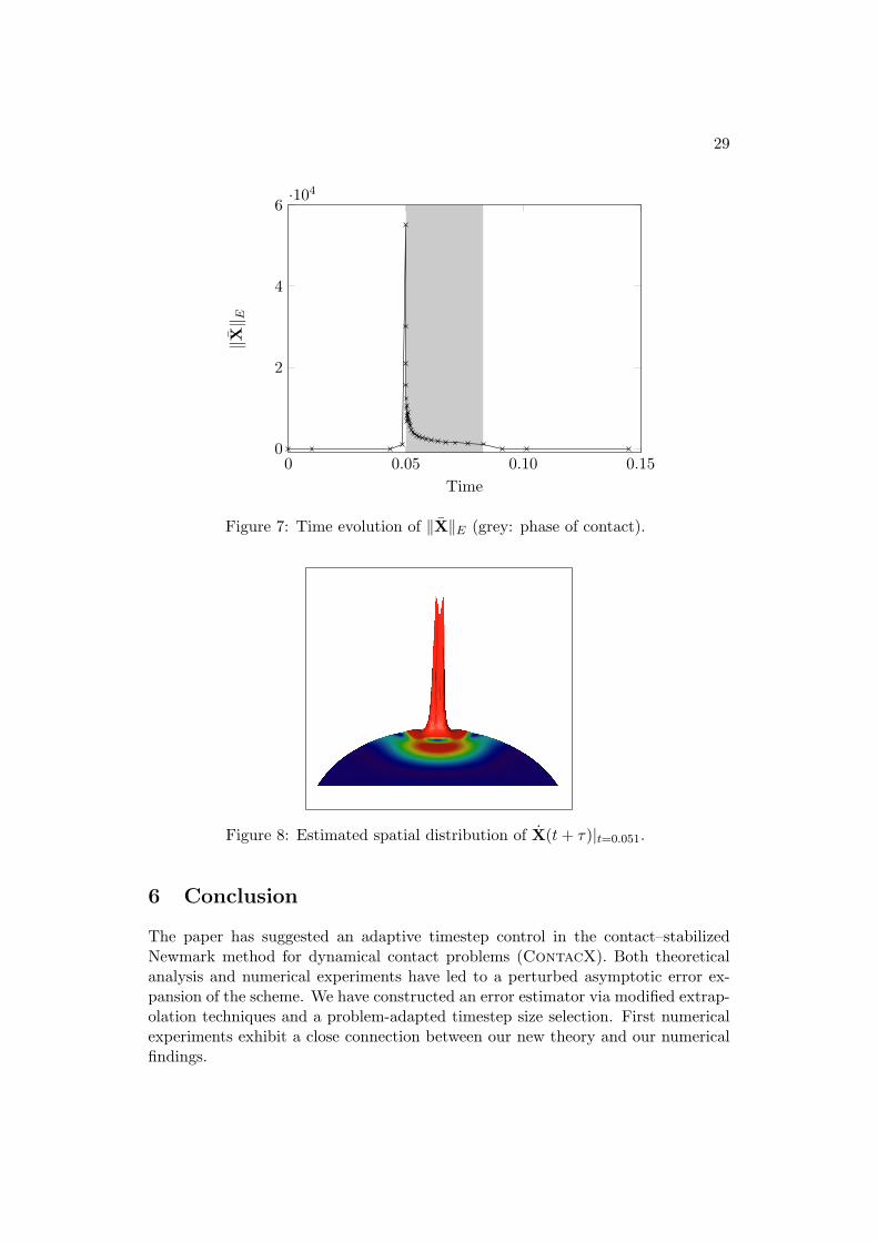
Figure 7 shows the time evolution of the physical energy norm of X. The normbecomes extremely large at the timepoint when the two bodies come into contact.In Figure 8, we see the spatial distribution of X for a fixed time. As expected,the quantity is located near the part of the possible contact boundaries where theactive set changes.

29

0.05 0.10 0.15

0

2

4

6·10

4

Time

‖X‖

E

0

Figure 7: Time evolution of ‖X‖E (grey: phase of contact).

Figure 8: Estimated spatial distribution of X(t + τ)|t=0.051.

6 Conclusion

The paper has suggested an adaptive timestep control in the contact–stabilizedNewmark method for dynamical contact problems (ContacX). Both theoreticalanalysis and numerical experiments have led to a perturbed asymptotic error ex-pansion of the scheme. We have constructed an error estimator via modified extrap-olation techniques and a problem-adapted timestep size selection. First numericalexperiments exhibit a close connection between our new theory and our numericalfindings.

30

Acknowledgment. The authors thank Martin Weiser, Zuse Institute Berlin, forhelpful discussions on the topic of this paper and Oliver Sander, FU Berlin, for hissupport with the multigrid solver for the stationary contact problems.

References

[1] J. Ahn and D. E. Stewart. Dynamic frictionless contact in linear viscoelasticity.IMA J. Numer. Anal., pages 1–29, 2008.

[2] P. Bastian, K. Birken, K. Johannsen, S. Lang, N. Neuß , H. Rentz–Reichert,and C. Wieners. UG – a flexible software toolbox for solving partial differentialequations. Comput. Vis. Sci., 1:27–40, 1997.

[3] P. Bastian, M. Blatt, A. Dedner, C. Engwer, R. Klofkorn, R. Kornhuber,M. Ohlberger, and O. Sander. A generic interface for parallel and adaptivescientific computing. Part II: Implementation and tests in dune. Computing,82(2–3):121–138, 2008.

[4] P. Bastian, M. Blatt, A. Dedner, C. Engwer, R. Klofkorn, M. Ohlberger, andO. Sander. A generic interface for parallel and adaptive scientific computing.Part I: Abstract framework. Computing, 82(2–3):103–119, 2008.

[5] P. Deuflhard and F. Bornemann. Scientific Computing with Ordinary Differ-ential Equations, volume 42 of Texts in Applied Mathematics. Springer, 2002.

[6] P. Deuflhard, R. Krause, and S. Ertel. A Contact-Stabilized Newmarkmethod for dynamical contact problems. Internat. J. Numer. Methods En-grg., 73(9):1274–1290, 2007.

[7] G. Duvaut and J. L. Lions. Inequalities in Mechanics and Physics. Springer,1976.

[8] C. Eck. Existenz und Regularitat der Losungen fur Kontaktprobleme mit Rei-bung. PhD thesis, Universitat Stuttgart, 1996.

[9] I. Ekeland and R. Temam. Convex Analysis and Variational Problems. North–Holland, Amsterdam, 1976.

[10] C. Graser and R. Kornhuber. Multigrid methods for obstacle problems.J. Comp. Math., 27:1–44, 2009.

[11] E. Hairer and C. Lubich. Asymptotic expansions of the global error of fixed-stepsize methods. Numer. Math., 45:345–360, 1982.

[12] E. Hairer, C. Lubich, and G. Wanner. Geometric Numerical Integration.Structure–Preserving Algorithms for Ordinary Differential Equations. Com-putational Mathematics. Springer, Berlin, Heidelberg, 2nd edition, 2006.

31

[13] C. Kane, E. A. Repetto, M. Ortiz, and J. E. Marsden. Finite element analysisof nonsmooth contact. Comput. Methods Appl. Mech. Engrg., 180:1–26, 1999.

[14] N. Kikuchi and J. T. Oden. Contact Problems in Elasticity. SIAM, Philadel-phia, 1988.

[15] C. Klapproth. Adaptive numerical integration for dynamical contact problems.PhD thesis. In preparation.

[16] C. Klapproth, P. Deuflhard, and A. Schiela. A perturbation result for dy-namical contact problems. Numer. Math. Theor. Meth. Appl., 2(3):237–257,2009.

[17] C. Klapproth, A. Schiela, and P. Deuflhard. Consistency results on Newmarkmethods for dynamical contact problems. Numer. Math., published online, 26March 2010. http://www.springerlink.com/content/72jq2430122253v2/.

[18] R. Kornhuber and R. Krause. Adaptive multilevel methods for Signorini’sproblem in linear elasticity. Comput. Vis. Sci., 4:9–20, 2001.

[19] R. Kornhuber, R. Krause, O. Sander, P. Deuflhard, and S. Ertel. A MonotoneMultigrid Solver for Two Body Contact Problems in Biomechanics. Comput.Vis. Sci., 11(1):3–15, 2008.

[20] R. Krause. Monotone Multigrid Methods for Signorini’s Problem with Fric-tion. PhD thesis, FU Berlin, 2000. http://www.diss.fu-berlin.de/diss/receive/FUDISS_thesis_000000000469.

[21] F. Mignot. Controle dans les inequations variationelles elliptiques. J. Funct.Anal., 22:130–185, 1976.

[22] E. Schechter. Handbook of Analysis and Its Foundations. Academic Press,1997.

[23] B. Wohlmuth and R. Krause. Monotone methods on nonmatching grids fornonlinear contact problems. SIAM J. Sci. Comput., 25(1):324–347, 2003.

[24] E. Zeidler. Nonlinear Functional Analysis and Applications II A/B. SpringerVerlag, 1990.