Adaptive Stochastic Galerkin Methods · 2010-09-21 · Adaptive Stochastic Galerkin Methods Claude...

Adaptive Stochastic Galerkin Methods

Claude Jeffrey GittelsonETH Zurich, Seminar for Applied MathematicsPhD. Thesis supervised by Prof. Ch. Schwab,supported by SNF Pro*Doc grant No. 200021-120290/1

Pro*Doc Workshop 2010 in Disentis

SPDE ONB FEM CDD END

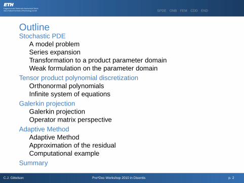
OutlineStochastic PDE

A model problemSeries expansionTransformation to a product parameter domainWeak formulation on the parameter domain

Tensor product polynomial discretizationOrthonormal polynomialsInfinite system of equations

Galerkin projectionGalerkin projectionOperator matrix perspective

Adaptive MethodAdaptive MethodApproximation of the residualComputational example

Summary

C.J. Gittelson Pro*Doc Workshop 2010 in Disentis p. 2


A model problemD ⊂ R

d Lipschitz, for ω ∈ Ω,

−∇ · (a(ω, x)∇u(ω, x)) = f(x) x ∈ D ,

u(ω, x) = 0 x ∈ ∂D .

Weak formulation: Find u(ω, x) ∈ H10 (D) such that

∫

D

a(ω, x)∇u(ω, x) · ∇v(x)dx =

∫

D

f(x)v(x)dx

for all v ∈ H10 (D).

Assume a(ω, x) is uniformly bounded,

0 < a− ≤ a(ω, x) ≤ a+ <∞ ∀x ∈ D , ∀ω ∈ Ω .



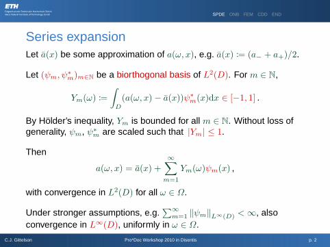
Series expansionLet a(x) be some approximation of a(ω, x), e.g. a(x) := (a− + a+)/2.

Let (ψm, ψ∗

m)m∈N be a biorthogonal basis of L2(D). For m ∈ N,

Ym(ω) :=

∫

D

(a(ω, x)− a(x))ψ∗

m(x)dx ∈ [−1, 1] .

By Hölder’s inequality, Ym is bounded for all m ∈ N. Without loss ofgenerality, ψm, ψ∗

m are scaled such that |Ym| ≤ 1.

Then

a(ω, x) = a(x) +

∞∑

m=1

Ym(ω)ψm(x) ,

with convergence in L2(D) for all ω ∈ Ω.

Under stronger assumptions, e.g.∑

∞

m=1 ‖ψm‖L∞(D) <∞, alsoconvergence in L∞(D), uniformly in ω ∈ Ω.



Transformation to a product parameter domainThe coefficients Ym(ω) of a(ω, x)− a(x) constitute a map

Y : Ω → Γ := [−1, 1]∞ , ω 7→ (Ym(ω))m∈N .

Define the parametric diffusion coefficient

a(y, x) := a(x) +

∞∑

m=1

ymψm(x) , y = (ym)m∈N ∈ Γ .

Then a(Y (ω), x) = a(ω, x) for all ω ∈ Ω.

For all y ∈ Γ , let u(y) ∈ H10 (D) solve

∫

D

a(y, x)∇u(y, x) · ∇v(x)dx =

∫

D

f(x)v(x)dx ∀v ∈ H10 (D) .

Then u(Y (ω), x) = u(ω, x) for all ω ∈ Ω.



Weak formulation on the parameter domain

Let πm be a probability measure on [−1, 1] for all m ∈ N, and

π :=

∞⊗

m=1

πm on (Γ,B(Γ )) .

If Y ∼ π, then (Ym)m are independent, and Ym ∼ πm.

Weak formulation: Find u ∈ L2π(Γ ;H

10 (D)) s.t. ∀v ∈ L2

π(Γ ;H10 (D)),

∫

Γ

∫

D

a(y, x)∇u(y, x) · ∇v(y, x)dxdπ(y) =

∫

Γ

∫

D

f(x)v(y, x)dxdπ(y) .

Continuous and coercive bilinear form on L2π(Γ ;H

10 (D)).

Product structure: L2π(Γ ;H

10 (D)) ∼= L2

π(Γ )⊗H10 (D).

deterministic space H10 (D),

stochastic space L2π(Γ ).



Orthonormal polynomialsOrthonormal polynomials w.r.t. πm satisfy a recursion P (m)

0 = 1,

β(m)n+1P

(m)n+1(ξ) = (ξ − α(m)

n )P (m)n (ξ)− β(m)

n P(m)n−1(ξ) .

Tensor product orthonormal polynomials

Pµ :=

∞⊗

m=1

P (m)µm

, µ ∈ Λ :=

µ ∈ NN

0 ; # suppµ <∞

,

i.e. Pµ(y) =∞∏

m=1

P (m)µm

(ym) =∏

m∈ suppµ

P (m)µm

(ym) for y ∈ Γ .

Theorem(Pµ)µ∈Λ is an orthonormal basis of L2

π(Γ ).



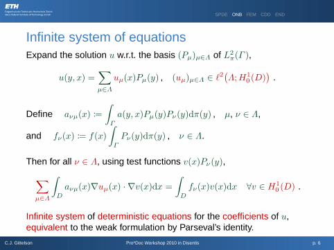
Infinite system of equationsExpand the solution u w.r.t. the basis (Pµ)µ∈Λ of L2

π(Γ ),

u(y, x) =∑

µ∈Λ

uµ(x)Pµ(y) , (uµ)µ∈Λ ∈ ℓ2(

Λ;H10 (D)

)

.

Define aνµ(x) :=

∫

Γ

a(y, x)Pµ(y)Pν(y)dπ(y) , µ, ν ∈ Λ,

and fν(x) := f(x)

∫

Γ

Pν(y)dπ(y) , ν ∈ Λ.

Then for all ν ∈ Λ, using test functions v(x)Pν (y),

∑

µ∈Λ

∫

D

aνµ(x)∇uµ(x) · ∇v(x)dx =

∫

D

fν(x)v(x)dx ∀v ∈ H10 (D) .

Infinite system of deterministic equations for the coefficients of u,equivalent to the weak formulation by Parseval’s identity.



Infinite system of equationsRecall

aνµ(x) =

∫

Γ

a(y, x)Pµ(y)Pν(y)dπ(y) , µ, ν ∈ Λ,

ξP (m)n (ξ) = β

(m)n+1P

(m)n+1(ξ) + α(m)

n P (m)n (ξ) + β(m)

n P(m)n−1(ξ),

a(y, x) = a(x) +

∞∑

m=1

ymψm(x).

Therefore, aνµ = 0 except for

aµµ(x) = a(x) +

∞∑

m=1

α(m)µm

ψm(x) ,

aµ,µ+ǫm(x) = aµ+ǫm,µ(x) = β(m)µm+1ψm(x) , m ∈ N .

In particular, no integrals over Γ need to be computed.



Galerkin projectionDefine a nested sequence of finite element spaces

0 = V0 ⊂ V1 ⊂ . . . ⊂ Vℓ ⊂ Vℓ+1 ⊂ . . . ⊂ H10 (D) .

For each µ ∈ Λ, select a space Vℓ(µ), and define

Vℓ :=

(vµ)µ∈Λ ; vµ ∈ Vℓ(µ) ∀µ ∈ Λ

⊂ ℓ2(

Λ;H10 (D)

)

.

Assume #µ ∈ Λ ; ℓ(µ) 6= 0 <∞, then dimVℓ <∞.

Galerkin projection: replace ℓ2(Λ;H10 (D)) by Vℓ in the infinite system

of equations for (uµ)µ∈Λ.

finite system of equations since Vℓ is finite dimensional.

well-posed by Lax–Milgram since the bilinear form is coercive.

quasi-optimal approximation in ℓ2(Λ;H10 (D)) ∼= L2

π(Γ ;H10 (D)).



Operator matrix perspectiveSemidiscrete setting VN := ℓ2(ΛN ;H1

0 (D)) for a ΛN ⊂ Λ, #ΛN = N .

Define the operator matrix AN ∈ L (H10 (D), H−1(D))N×N ,

AN := (Aνµ)ν,µ∈ΛN, Aνµv := −∇ · (aνµ∇v) ,

and the vector fN := (fν)ν∈ΛN∈ H−1(D)N .

The Galerkin projection uN ∈ H10 (D)N is the solution of

ANuN = fN .

Iterative solution, e.g. by PCG, with preconditioner AN := diag(A),Av := −∇ · (a∇v) consists of applications of Aνµ and A−1.

The matrix AN is sparse,

nnz(AN ) ≤ (1 + 2λ(ΛN))N

for the average index length λ(ΛN ) := 1N

∑

µ∈ΛN#suppµ.



Adaptive MethodIterative adaptive method u

(0)N

:= 0, Λ(0)N

:= ∅

1. r(k)N

:= Residual(u(k)N ) approximate f −Au

(k)N

2. Λ(k+1)N

:= Refine(Λ(k)N , r

(k)N ) refine the discretization

3. u(k+1)N

:= Galerkin(Λ(k+1)N ) Galerkin sol. in ℓ2(Λ(k+1)

N ;H10 (D))

LemmaIf

∥

∥

∥

∥

(f −Au(k)N )

∣

∣

∣

Λ(k+1)N

∥

∥

∥

∥

ℓ2(Λ;H−1)

≥ ϑ∥

∥

∥f −Au

(k)N

∥

∥

∥

ℓ2(Λ;H−1), then

∥

∥

∥u− u

(k+1)N

∥

∥

∥

AAA≤

√

1− κ(A)−1ϑ2∥

∥

∥u− u

(k)N

∥

∥

∥

AAA.

In particular, the iteration converges in the energy norm.



Approximation of the residual

GoalFor w =

∑

µ∈ΛNwµPµ, approximate the residual

r(w) := f +∇ · (a∇w) +

∞∑

m=1

∇ · (ψm∇w) .

PartitionΛN = Λ

[1]N ⊔ Λ

[2]N ⊔ · · · ⊔ Λ

[J]N ,

where Λ[1J]N contains µ ∈ ΛN with the largestsmallest |wµ|H1

0 (D).

For w[j] := w|Λ

[j]N

and M1 ≥M2 ≥ · · · ≥MJ ≥ 0,

r(w) ≈ rN (w) := f +∇ · (a∇w) +J∑

j=1

Mj∑

m=1

∇ · (ψm∇w[j]) .



Computational exampleModel problem

D = (0, 1)

f(x) = x

a(x) = 1, i.e. A = −∆

ψm(x) = cm−4 sin(mπx), scaled such that c∑

∞

m=1m−4 = 5

6

πm is the uniform distribution on [−1, 1], i.e. dπm(ym) = 12dym

P(m)n are Legendre polynomials

Linear finite element discretization,

Single level fixed finite element space Vℓ ⊂ H10 (D) for all µ ∈ ΛN

and all iterations k

Multi-level different Vℓ for each µ ∈ ΛN and k ∈ N, determined aposteriori in the refinement step



Computational example

100

101

102

103

104

105

10−5

10−4

10−3

10−2

10−1

Number of Degrees of Freedom

Error

inℓ2(Λ

;H1 0)

Multi-levelSingle level



Computational example

101

102

103

104

105

106

10−5

10−4

10−3

10−2

10−1

Estimated Computational Cost

Error

inℓ2(Λ

;H1 0)

Multi-levelSingle level



SummaryTensor products of orthonormal polynomials form an orthonormalbasis (Pµ)µ∈Λ of L2

π(Γ ) for the infinite product domainΓ = [−1, 1]∞ and infinite product measure π =

⊗

∞

m=1 πm.

Expanding the solution u w.r.t. this basis, a stochastic boundaryvalue problem is recast as an infinite system of deterministicequations.

Galerkin projections can be computed by standard iterativemethods applied to a sparse operator matrix.

Adaptive wavelet techniques applied to the basis (Pµ)µ∈Λ can beused to determine appropriate sets ΛN of active indices andfinite element spaces Vℓ(µ), µ ∈ ΛN , during the solution process.

Thank you for your attention!


Adaptive Stochastic Galerkin Methods · 2010-09-21 · Adaptive Stochastic Galerkin Methods Claude...

Documents

Transcript of Adaptive Stochastic Galerkin Methods · 2010-09-21 · Adaptive Stochastic Galerkin Methods Claude...