ADAPTIVE NOISE CANCELLATION USING MODIFIED SIMULATED ...
117
ADAPTIVE NOISE CANCELLATION USING MODIFIED SIMULATED ANNEALING ALGORITHM KEVIN MUNENE MWONGERA MASTER OF SCIENCE (Telecommunication Engineering) JOMO KENYATTA UNIVERSITY OF AGRICULTURE AND TECHNOLOGY 2021
Transcript of ADAPTIVE NOISE CANCELLATION USING MODIFIED SIMULATED ...
ADAPTIVE NOISE CANCELLATION USING
MODIFIED SIMULATED ANNEALING
ALGORITHM
KEVIN MUNENE MWONGERA
MASTER OF SCIENCE
(Telecommunication Engineering)
JOMO KENYATTA UNIVERSITY OF
AGRICULTURE AND TECHNOLOGY
2021

Adaptive noise cancellation using modified simulated
annealing algorithm
Kevin Munene Mwongera
A thesis submitted in partial fulfillment of the
requirement for the Degree of Master of Science in
Telecommunication Engineering of the Jomo Kenyatta
University of Agriculture and Technology
2021

DECLARATION
This thesis is my original work and has not been presented for a degree in any
other university.
Signature: Date:
Kevin Munene Mwongera
This thesis has been submitted for examination with our approval as the univer-
sity supervisors
Signature: Date:
Dr Kibet P Langat
JKUAT, Kenya
Signature: Date:
Dr E N Ndungu
JKUAT, Kenya
ii
DEDICATION
This thesis is dedicated to my parents for their immense support, encouragement
and counsel throughout my academic life. Also, this thesis is dedicated to my wife,
Milda who has been a great source of encouragement and inspiration throughout
my period of study.
iii
ACKNOWLEDGMENTS
Foremost, I hereby thank God who granted me this opportunity to contribute
something to the field of knowledge in Telecommunication Engineering. I ac-
knowledge the assistance of my supervisors Dr. Kibet Langat and Dr E N
Ndungu for their continuous support of my Masters studies and accompanying
research.Their guidance assisted me immensely throughout the period of study.
I also thank the department of Telecommunication Engineering Faculty, JKUAT
for the guidance and support during the research period.
I also thank sincerely my three mentors and colleagues Mr Macharia, Mr Onim
and Mrs Onyango for their advise, motivation and their input towards the com-
pletion of this thesis.
iv
TABLE OF CONTENTS
DECLARATION . . . . . . . . . . . . . . . . . . . . . . . . . . . . . ii
DEDICATION . . . . . . . . . . . . . . . . . . . . . . . . . . . . . . iii
ACKNOWLEDGEMENTS . . . . . . . . . . . . . . . . . . . . . . . iv
TABLE OF CONTENTS . . . . . . . . . . . . . . . . . . . . . . . . v
LIST OF TABLES . . . . . . . . . . . . . . . . . . . . . . . . . . . . viii
LIST OF FIGURES . . . . . . . . . . . . . . . . . . . . . . . . . . . ix
LIST OF APPENDICES . . . . . . . . . . . . . . . . . . . . . . . . xiv
LIST OF ABBREVIATIONS . . . . . . . . . . . . . . . . . . . . . . xv
ABSTRACT . . . . . . . . . . . . . . . . . . . . . . . . . . . . . . . . xvi
CHAPTER ONE . . . . . . . . . . . . . . . . . . . . . . . . . . . . . 1
INTRODUCTION . . . . . . . . . . . . . . . . . . . . . . . . . . . . 1
1.1 Background . . . . . . . . . . . . . . . . . . . . . . . . . . . . . . 1
1.2 Problem statement . . . . . . . . . . . . . . . . . . . . . . . . . . 2
1.3 Justification . . . . . . . . . . . . . . . . . . . . . . . . . . . . . . 3
1.4 Objectives . . . . . . . . . . . . . . . . . . . . . . . . . . . . . . . 3
1.4.1 Main objective . . . . . . . . . . . . . . . . . . . . . . . . 3
1.4.2 Specific objectives . . . . . . . . . . . . . . . . . . . . . . . 3
1.5 Thesis organization . . . . . . . . . . . . . . . . . . . . . . . . . . 4
CHAPTER TWO . . . . . . . . . . . . . . . . . . . . . . . . . . . . . 5
LITERATURE REVIEW . . . . . . . . . . . . . . . . . . . . . . . . 5
2.1 Adaptive Noise Cancellation . . . . . . . . . . . . . . . . . . . . . 5
v
2.2 Adaptive Noise cancellation performance measures . . . . . . . . . 6
2.2.1 Convergence rate . . . . . . . . . . . . . . . . . . . . . . . 6
2.2.2 Computational complexity . . . . . . . . . . . . . . . . . . 7
2.3 Adaptive noise cancellation solutions in literature . . . . . . . . . 7
2.3.1 Use of LMS and NLMS algorithms . . . . . . . . . . . . . 7
2.3.2 Use of artificial intelligence algorithms . . . . . . . . . . . 9
2.4 Simulated Annealing algorithm . . . . . . . . . . . . . . . . . . . 11
2.4.1 Introduction . . . . . . . . . . . . . . . . . . . . . . . . . . 11
2.4.2 Algorithm operation . . . . . . . . . . . . . . . . . . . . . 11
2.4.3 Operational elements . . . . . . . . . . . . . . . . . . . . . 12
2.4.4 One Dimensional Minimization problem . . . . . . . . . . 12
2.4.5 SA algorithm strengths . . . . . . . . . . . . . . . . . . . . 14
2.4.6 SA algorithm improvements . . . . . . . . . . . . . . . . . 16
2.4.7 SA Versus Other AI Algorithms . . . . . . . . . . . . . . . 17
2.5 Summary . . . . . . . . . . . . . . . . . . . . . . . . . . . . . . . 18
CHAPTER THREE . . . . . . . . . . . . . . . . . . . . . . . . . . . 19
METHODOLOGY . . . . . . . . . . . . . . . . . . . . . . . . . . . . 19
3.1 Development of an adaptive noise cancellation model . . . . . . . 19
3.1.1 ANC model formulation . . . . . . . . . . . . . . . . . . . 19
3.1.2 Cost function formulation . . . . . . . . . . . . . . . . . . 19
3.1.3 Correlation performance measure . . . . . . . . . . . . . . 21
3.1.4 Euclidean distance performance measure . . . . . . . . . . 22
3.2 Simulated annealing algorithm improvement . . . . . . . . . . . . 22
3.2.1 Acceptance Probability . . . . . . . . . . . . . . . . . . . . 23
3.2.2 Cooling scheme . . . . . . . . . . . . . . . . . . . . . . . . 26
3.3 Application and analysis of the modified SA algorithm in adaptive
noise cancellation . . . . . . . . . . . . . . . . . . . . . . . . . . . 30
vi
3.3.1 Noise cancellation framework . . . . . . . . . . . . . . . . 30
3.3.2 Speech signal framework . . . . . . . . . . . . . . . . . . . 31
3.4 Performance comparison: SA algorithm against standard LMS and
NLMS algorithms in adaptive noise cancellation. . . . . . . . . . . 31
3.4.1 Utilized signal formats . . . . . . . . . . . . . . . . . . . . 32
3.4.2 Performance metrics . . . . . . . . . . . . . . . . . . . . . 38
3.5 Summary . . . . . . . . . . . . . . . . . . . . . . . . . . . . . . . 38
CHAPTER FOUR . . . . . . . . . . . . . . . . . . . . . . . . . . . . 39
RESULTS AND DISCUSSION . . . . . . . . . . . . . . . . . . . . . 39
4.1 Comparison of the improved SA algorithm against the standard
SA algorithm in adaptive noise cancellation . . . . . . . . . . . . 39
4.2 Comparison of the improved simulated annealing algorithm in adap-
tive noise cancellation with standard SA, NLMS and LMS algorithms 42
4.2.1 Sinusoidal waveform . . . . . . . . . . . . . . . . . . . . . 43
4.2.2 Irregular waveform . . . . . . . . . . . . . . . . . . . . . . 63
4.2.3 Electrocardiogram waveform . . . . . . . . . . . . . . . . . 72
4.3 Summary . . . . . . . . . . . . . . . . . . . . . . . . . . . . . . . 80
CHAPTER FIVE . . . . . . . . . . . . . . . . . . . . . . . . . . . . . 81
CONCLUSION AND RECOMMENDATIONS . . . . . . . . . . . 81
5.1 Conclusion . . . . . . . . . . . . . . . . . . . . . . . . . . . . . . . 81
5.1.1 Highlights and deductions . . . . . . . . . . . . . . . . . . 81
5.1.2 Contribution . . . . . . . . . . . . . . . . . . . . . . . . . 82
5.2 Recommendations . . . . . . . . . . . . . . . . . . . . . . . . . . . 82
REFERENCES . . . . . . . . . . . . . . . . . . . . . . . . . . . . . . 83
APPENDICES . . . . . . . . . . . . . . . . . . . . . . . . . . . . . . 90
vii
LIST OF TABLES
Table 3.1: Exponential/ linear functions comparison. . . . . . . . 26
Table 3.2: Selected cooling schedules in literature: constant values
used. . . . . . . . . . . . . . . . . . . . . . . . . . . . . 30
Table 3.3: Selected cooling schedules in literature: computation time. 30
Table 4.4: Comparative correlation values. . . . . . . . . . . . . . 42
Table 4.5: Comparative correlation values. . . . . . . . . . . . . . 49
Table 4.6: Signal correlation comparison . . . . . . . . . . . . . . 71
Table 4.7: Iregular waveform Euclidean distance comparison . . . 72
Table 4.8: Electrocardiogram waveform Euclidean distance com-
parison . . . . . . . . . . . . . . . . . . . . . . . . . . . 80
viii
LIST OF FIGURES
Figure 2.1: Adaptive noise canceller . . . . . . . . . . . . . . . . . 6
Figure 2.2: SA algorithm operation . . . . . . . . . . . . . . . . . 13
Figure 2.3: Typical one-dimension minimization problem . . . . . 13
Figure 2.4: Initial iteration solution (dot symbol) as compared against
the optimal solution (asterisk symbol). . . . . . . . . . 14
Figure 2.5: Second iteration solution (dot symbol) as compared
against the optimal solution (asterisk symbol). . . . . 15
Figure 2.6: Third iteration solution (dot symbol) as compared against
the optimal solution (asterisk symbol). . . . . . . . . . 15
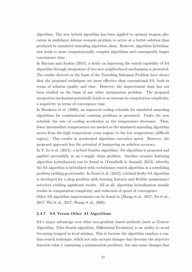
Figure 2.7: Fourth iteration solution (dot symbol) as compared
against the optimal solution (asterisk symbol). . . . . 15
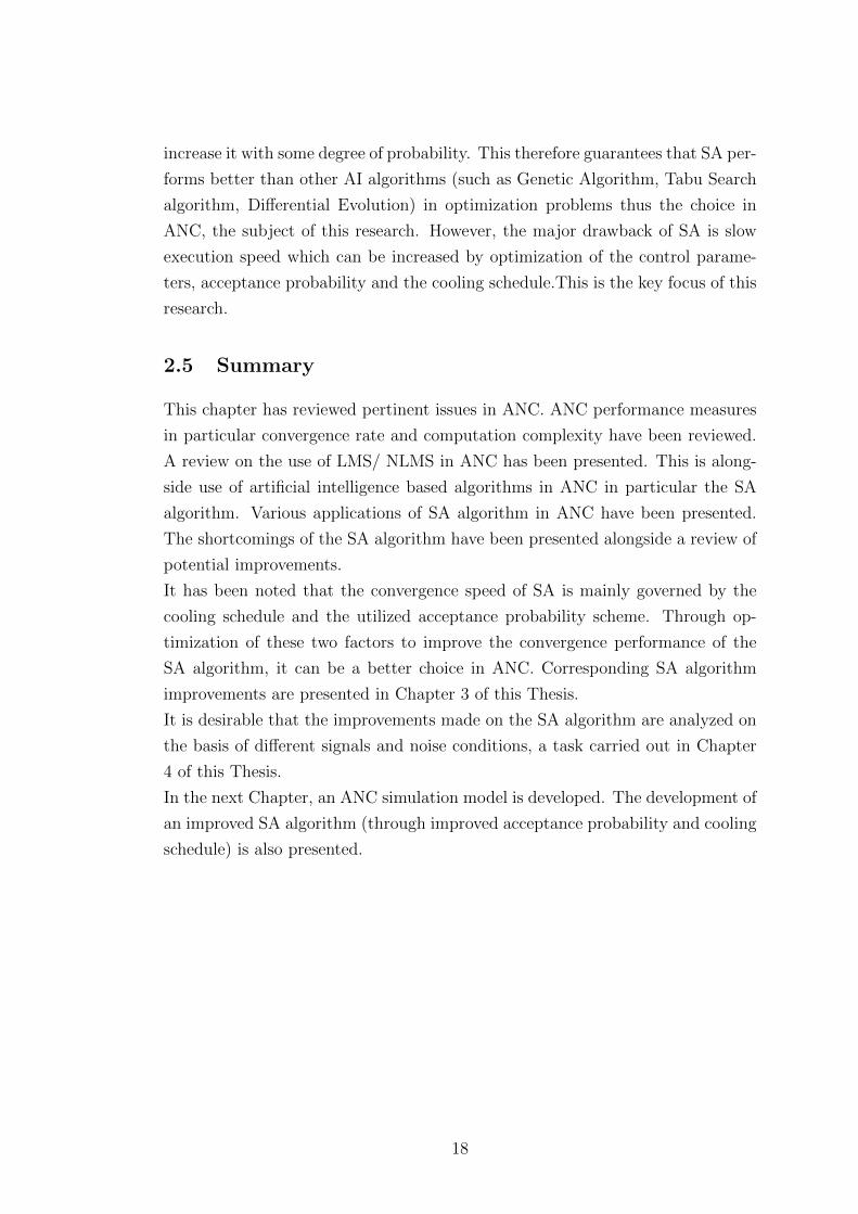
Figure 2.8: Final iteration solution (dot symbol) as compared against
the optimal solution (asterisk symbol). . . . . . . . . . 16
Figure 3.9: SA algorithm flow chart . . . . . . . . . . . . . . . . . 24
Figure 3.10: Exponential/ linear functions comparison. . . . . . . . 25
Figure 3.11: Developed acceptance probability scheme (Data col-
lected from Matlab simulations). . . . . . . . . . . . . 27
Figure 3.12: Developed cooling schedule (graph derived from Equa-
tion 3.19). . . . . . . . . . . . . . . . . . . . . . . . . 28
Figure 3.13: Selected cooling schedules in literature. . . . . . . . . 29
Figure 3.14: Adaptive noise cancellation process. . . . . . . . . . . 31
Figure 3.15: Maternal Electrocardiogram Signal (noise free). . . . . 33
Figure 3.16: Fetal Electrocardiogram Signal (noise free). . . . . . . 34
Figure 3.17: Measured Fetal Electrocardiogram Signal . . . . . . . 35
Figure 3.18: Reference Electrocardiogram Signal . . . . . . . . . . 36
Figure 3.19: Sinusoidal waveform . . . . . . . . . . . . . . . . . . . 37
Figure 3.20: Irregular waveform . . . . . . . . . . . . . . . . . . . . 37
ix
Figure 4.21: Comparison of the results obtained upon adaptive noise
cancellation in a speech signal problem using improved
and standard SA algorithms: Audio Channel 1. . . . . 40
Figure 4.22: Comparison of the results obtained upon adaptive noise
cancellation in a speech signal problem using improved
and standard SA algorithms: Audio Channel 2. . . . . 41
Figure 4.23: A graph portraying the correlation values presented in
Table 4.1. . . . . . . . . . . . . . . . . . . . . . . . . . 42
Figure 4.24: Desired signal: Sinusoidal waveform. s(n) = 5∗sin(12∗
n) where n = 1 : 0.025 : 4.5 . . . . . . . . . . . . . . . 43
Figure 4.25: Noise signal: Sinusoidal waveform with additive gaus-
sian noise. no(n) = sin(300 ∗ n) + awgn where n = 1 :
0.025 : 4.5 . . . . . . . . . . . . . . . . . . . . . . . . . 44
Figure 4.26: Corrupted signal: d(n) = 5∗ sin(12∗n)+sin(300∗n)+
awgn. . . . . . . . . . . . . . . . . . . . . . . . . . . . 45
Figure 4.27: Reference signal (highly correlated to the noise signal):
x(n) = sin(300 ∗ n) + awgnReference. . . . . . . . . . . 46
Figure 4.28: A comparison between the reference and noise signals. 46
Figure 4.29: Comparison (against the desired signal) of the results
obtained upon adaptive noise cancellation using the
improved SA, standard SA, LMS and NLMS algorithms. 47
Figure 4.30: Comparison of the results obtained upon adaptive noise
cancellation using the improved SA, standard SA, LMS
and NLMS algorithms. . . . . . . . . . . . . . . . . . 48
Figure 4.31: A graph portraying the correlation values presented in
Table 4.2. . . . . . . . . . . . . . . . . . . . . . . . . . 49
Figure 4.32: A comparison between the reference and noise signals. 50
Figure 4.33: SA algorithm result . . . . . . . . . . . . . . . . . . . 50
x

Figure 4.34: Desired signal: Sinusoidal waveform. s(n) = 5∗ sin(6∗
n) where n = 1 : 0.025 : 4.5 . . . . . . . . . . . . . . . 51
Figure 4.35: Noise signal: Sinusoidal waveform with additive gaus-
sian noise. no(n) = 2 ∗ sin(300 ∗ n) + awgn where
n = 1 : 0.025 : 4.5 . . . . . . . . . . . . . . . . . . . . 52
Figure 4.36: Corrupted signal: d(n) = 5 ∗ sin(6 ∗ n) + 2 ∗ sin(300 ∗
n) + awgn. . . . . . . . . . . . . . . . . . . . . . . . . 53
Figure 4.37: Reference signal (highly correlated to the noise signal):
x(n) = sin(300 ∗ n) + awgnReference. . . . . . . . . . . 54
Figure 4.38: A comparison between the reference and noise signals. 54
Figure 4.39: Comparison (against the desired signal) of the results
obtained upon adaptive noise cancellation using the
improved SA, standard SA, LMS and NLMS algorithms. 55
Figure 4.40: Comparison of the results obtained upon adaptive noise
cancellation using the improved SA, standard SA, LMS
and NLMS algorithms. . . . . . . . . . . . . . . . . . 56
Figure 4.41: Desired signal: Sinusoidal waveform. s(n) = 5∗ sin(2∗
n) where n = 1 : 0.025 : 4.5 . . . . . . . . . . . . . . . 57
Figure 4.42: Noise signal: Sinusoidal waveform with additive gaus-
sian noise. no(n) = 2 ∗ sin(300 ∗ n) + awgn where
n = 1 : 0.025 : 4.5 . . . . . . . . . . . . . . . . . . . . 58
Figure 4.43: Corrupted signal: d(n) = 5 ∗ sin(2 ∗ n) + 2 ∗ sin(300 ∗
n) + awgn. . . . . . . . . . . . . . . . . . . . . . . . . 59
Figure 4.44: Reference signal (highly correlated to the noise signal):
x(n) = 2 ∗ sin(300 ∗ n) + awgnReference. . . . . . . . . . 60
Figure 4.45: A comparison between the reference and noise signals. 60
xi
Figure 4.46: Comparison (against the desired signal) of the results
obtained upon adaptive noise cancellation using the
improved SA, standard SA, LMS and NLMS algorithms. 61
Figure 4.47: Comparison of the results obtained upon adaptive noise
cancellation using the improved SA, standard SA, LMS
and NLMS algorithms. . . . . . . . . . . . . . . . . . 62
Figure 4.48: Desired signal: Irregular waveform. s(n) = rand(n; [−2.5 :
2.5]) where n = 1 : 0.2 : 4.5 . . . . . . . . . . . . . . . 64
Figure 4.49: Noise signal: Random waveform with additive gaussian
noise. n0(n) = rand(n; [−0.5 : 0.5]) + awgnnoise where
n = 1 : 0.02 : 4.5 . . . . . . . . . . . . . . . . . . . . . 65
Figure 4.50: Corrupted signal: d(n) = rand(n; [−2.5 : 2.5])+rand(n; [−0.5 :
0.5]) + awgnnoise. . . . . . . . . . . . . . . . . . . . . . 65
Figure 4.51: Reference signal (highly correlated to the noise signal):
x(n) = n0(n) + awgnref . . . . . . . . . . . . . . . . . . 66
Figure 4.52: A comparison of the reference and noise signals. . . . 67
Figure 4.53: Comparison (against the desired signal) of the results
obtained upon adaptive noise cancellation using the
improved SA, standard SA, LMS and NLMS algorithms. 68
Figure 4.54: Comparison of the results obtained upon adaptive noise
cancellation using the improved SA, standard SA, LMS
and NLMS algorithms. . . . . . . . . . . . . . . . . . 69
Figure 4.55: Algorithm performance comparison. . . . . . . . . . . 70
Figure 4.56: Point by point Euclidean distances comparison . . . . 71
Figure 4.57: Desired signal: Typical fetal electrocardiogram signal. 73
Figure 4.58: Noise signal: Maternal heartbeat and sinusoidal noise. 73
Figure 4.59: Noise corrupted fetal electrocardiogram signal. . . . . 74
Figure 4.60: Reference signal (highly correlated to the noise signal). 74
xii

Figure 4.61: A comparison of the reference and noise signals. . . . 75
Figure 4.62: Comparison (against the desired signal) of the results
obtained upon adaptive noise cancellation using the
improved SA, standard SA, LMS and NLMS algorithms. 76
Figure 4.63: Comparison of the results obtained upon adaptive noise
cancellation using the improved SA, standard SA, LMS
and NLMS algorithms. . . . . . . . . . . . . . . . . . 77
Figure 4.64: Algorithm performance comparison . . . . . . . . . . . 78
Figure 4.65: Euclidean distances comparison . . . . . . . . . . . . . 79
Figure 4.66: Average Euclidean distances comparison . . . . . . . . 79
xiii

LIST OF APPENDICES
Appendix I: Published Work........................................................... 91
Appendix II: Matlab Code................................................................ 92
xiv
LIST OF ABBREVIATIONS
AAC Advanced Audio Coding
ABC Artificial Bee Colony
AI Artificial Intelligence
ANC Adaptive Noise Cancellation
ANFIS Adaptive Neuro Fuzzy Inference System
AWGN Additive White Gaussian Noise
CS Cuckoo Search
DTW Dynamic Time Warping
ECG Electro Cardio Gram
EDF Evolutionary Digital Filtering
FIR Finite Impulse Response
GA Genetic Algorithm
IIR Infinite Impulse Response
LMS Least Mean Square
M4A MPEG-4 Audio
ME Maximum Error
MMSE Minimum Mean Square Error
MSE Mean Square Error
NLMS Normalized Least Mean Squares
PSO Particle Swarm Optimization
RLS Recursive Least Squares
SA Simulated Annealing
SINR Signal to Interference and Noise Ratio
SNR Signal to Noise Ratio
SSNR Segmental Signal to Noise Ratio
WLMS Wavelet transform domain Least Mean Square
xv
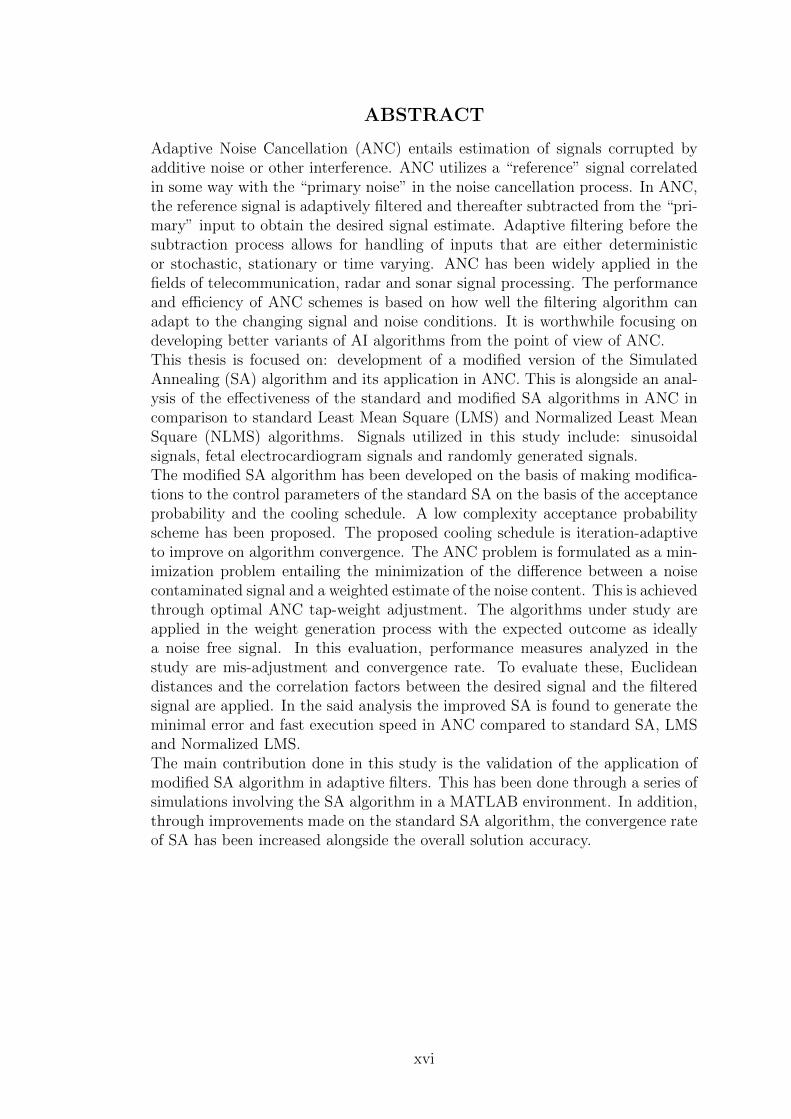
ABSTRACT
Adaptive Noise Cancellation (ANC) entails estimation of signals corrupted byadditive noise or other interference. ANC utilizes a “reference” signal correlatedin some way with the “primary noise” in the noise cancellation process. In ANC,the reference signal is adaptively filtered and thereafter subtracted from the “pri-mary” input to obtain the desired signal estimate. Adaptive filtering before thesubtraction process allows for handling of inputs that are either deterministicor stochastic, stationary or time varying. ANC has been widely applied in thefields of telecommunication, radar and sonar signal processing. The performanceand efficiency of ANC schemes is based on how well the filtering algorithm canadapt to the changing signal and noise conditions. It is worthwhile focusing ondeveloping better variants of AI algorithms from the point of view of ANC.This thesis is focused on: development of a modified version of the SimulatedAnnealing (SA) algorithm and its application in ANC. This is alongside an anal-ysis of the effectiveness of the standard and modified SA algorithms in ANC incomparison to standard Least Mean Square (LMS) and Normalized Least MeanSquare (NLMS) algorithms. Signals utilized in this study include: sinusoidalsignals, fetal electrocardiogram signals and randomly generated signals.The modified SA algorithm has been developed on the basis of making modifica-tions to the control parameters of the standard SA on the basis of the acceptanceprobability and the cooling schedule. A low complexity acceptance probabilityscheme has been proposed. The proposed cooling schedule is iteration-adaptiveto improve on algorithm convergence. The ANC problem is formulated as a min-imization problem entailing the minimization of the difference between a noisecontaminated signal and a weighted estimate of the noise content. This is achievedthrough optimal ANC tap-weight adjustment. The algorithms under study areapplied in the weight generation process with the expected outcome as ideallya noise free signal. In this evaluation, performance measures analyzed in thestudy are mis-adjustment and convergence rate. To evaluate these, Euclideandistances and the correlation factors between the desired signal and the filteredsignal are applied. In the said analysis the improved SA is found to generate theminimal error and fast execution speed in ANC compared to standard SA, LMSand Normalized LMS.The main contribution done in this study is the validation of the application ofmodified SA algorithm in adaptive filters. This has been done through a series ofsimulations involving the SA algorithm in a MATLAB environment. In addition,through improvements made on the standard SA algorithm, the convergence rateof SA has been increased alongside the overall solution accuracy.
xvi
CHAPTER ONE
INTRODUCTION
1.1 Background
Distortion of a signal of interest by other undesired signals (noise) is a problem
encountered in many signal processing applications. In most applications, the
desired signal has changing characteristics which require an update in the filter
coefficients for a good performance in signal extraction. Since conventional digital
filters with fixed coefficients do not have the ability to update their coefficients,
adaptive digital filters are used to cancel the noise.
Adaptive Noise Cancellation (ANC) filters have been of immense interest due to
their self-reconfiguration properties (Haykin, 2002). When some prior knowledge
about the statistics of a signal under consideration is available, an optimal fil-
ter for such application can be easily developed (for instance the Wiener Filter
which minimizes the respective Mean Square Error (MSE)). MSE is the difference
between the developed optimal filter output and the desired response (Haykin,
2002). If this prior knowledge is unavailable, adaptive filtering algorithms have
the ability to adapt the corresponding filter coefficients to be well-matched with
the involved signal statistics. Adaptive filtering/ noise cancellation algorithms
have been used in many fields such as signal processing, communications systems
and control systems (Haykin, 2002).
Adaptive filtering process consists of two major steps; the filtering process which
generates an output signal (response) from the input signal, and an adaptation
process; which adjusts the filter coefficients intelligently in order to result in an
optimal output. There are a number of filter structures and adaptive filtering
algorithms that are used in adaptive filtering applications. Such structures in-
clude: adaptive system identification, adaptive noise cancellation, adaptive linear
prediction, adaptive inverse system configurations. Of particular interest in this
thesis is the adaptive noise cancellation configuration. Adaptive noise cancella-
tion is essential in a broad range of communication and automation/ sensor based
systems.
Adaptive filters are usually classified into two main categories depending on their
impulse response: Finite Impulse Response (FIR) adaptive filter and to a limited
extent Infinite Impulse Response (IIR) adaptive filter (Bellanger, 2001). An FIR
adaptive filter’s impulse response has a finite duration since it goes to zero after a
finite time whereas an IIR adaptive filter has an internal feedback mechanism and
continues to respond indefinitely. FIR filters are generally preferred for adaptive
filtering due to their inherent stability.
1
General research and applications of adaptive noise cancellation can be found in
(Z.-K. Yang et al., 2020; Mehmood et al., 2019; Murugendrappa et al., 2020;
Thunga & Muthu, 2020; Wei & Shao, 2019; Miyahara et al., 2019; Maurya et al.,
2019; Balaji et al., 2020; Dixit & Nagaria, 2019; Patnaik et al., 2020).
1.2 Problem statement
Adaptive filters have a wide range of applications in a variety of engineering ap-
plications which basically lie in four broad categories namely: Interference cance-
lation, system identification, inverse system modeling as well as signal prediction.
Interference cancelation is the focus of this research.
In all these applications the performance and efficiency of the noise cancelation
scheme is based on how well the adaptive algorithm can adapt to the changing
signal and noise conditions. This therefore means that adaptive filters are basi-
cally governed by the weights adaptation process for the algorithms utilized in
the noise cancelation process.
Previous research has been centered and done in application of gradient based
algorithm like Least Mean Squares (LMS) in the weights adaptation process which
have shortcomings when applied to signals which have multiple maxima and/or
minima since in the process of exploring the solution space they may get trapped
in a local solution thus failing to generate the desired results. No much focus has
been placed on guided random search algorithms such as Simulated Annealing
(SA) and Genetic algorithm (GA) in ANC. An application of AI in ANC can
be found in (Xia et al., 2008), wherein the Particle Swarm Optimization (PSO)
algorithm has been utilized. However, PSO is found to suffer from premature
convergence. An application of AI in ANC can be found in (Chang & Chen, 2010),
wherein the GA algorithm has been utilized. However, GA is found to suffer
from slow convergence rate. Focus ought to be particularly on developing better
variants of AI algorithms from the point of view of adaptive noise cancellation.
SA is known to generate optimal results in global optimization problems but it
faces a major setback of having very slow convergence rate. This study looks into
the application of standard SA in ANC as well as explores the control param-
eters to increase convergence rate and reduce misadjustment. The influence of
the acceptance probability and the cooling schedule on the algorithm annealing
process are control parameters that are the basis of this study.
2
1.3 Justification
The process of obtaining viable adaptive filter weights as quickly as possible in
noise cancelation schemes is crucial depending on the application and require-
ments at hand. Classical algorithms such as the Least Mean Squares (LMS)
algorithm fail in satisfying this requirement, hence the growing research into use
of Artificial Intelligence(AI) algorithms.
Use of AI in ANC adaptive weight evaluation is an active area of research with
Genetic Algorithm receiving the major research focus. This is unlike SA which
has had fewer studies conducted in application to optimization problems. SA is
a robust versatile algorithm due to its inherent nature of expansive search of the
solution space which guarantees a statistical optimal solution to an optimization
problem. This algorithm also has fewer number of control parameters that are
used in tuning its performance compared to other heuristic algorithms like GA.
Weight adaptation process in ANC requires a solution which is easily programmable,
This has a direct relationship with the number of control parameters and number
of cost evaluations thus SA proves to be the best candidate for this since the
key control parameters are the cooling schedule and the acceptance probability
schemes.
The major drawback for Simulated Annealing is the slow execution speed, though
the algorithm is said to be a ‘quick starter’ its overall execution speed is low
compared to other AI algorithms like GA. Thus there is need to work on improving
the execution speed for SA while at the same time comparing its efficiency in the
weights adaptation process to other conventional algorithms such as LMS,and
Normalized Least Mean Squares (NLMS).
1.4 Objectives
1.4.1 Main objective
To develop an improved version of the Simulated Annealing (SA) algorithm and
apply it in adaptive noise cancellation using simulation models in Matlab.
1.4.2 Specific objectives
1. To develop an adaptive noise cancellation model in Matlab.
2. To develop a modified version of the SA algorithm.
3
3. To apply standard SA algorithm and its modified version in the developed
ANC models and compare the effectiveness of the modified version in ANC
over the standard SA algorithm.
4. To analyze the effectiveness of the standard and modified Simulated An-
nealing algorithm in ANC in comparison to standard LMS and NLMS al-
gorithms.
1.5 Thesis organization
Chapter 1 lays down an introduction to the work carried out in the thesis. Chap-
ter 2 lays down a review of various works done by other researchers in the ANC
problem as well as a review of the SA algorithm. Chapter 3 (Methodology) de-
scribes the development of an ANC model and the development of an improved
SA algorithm. Chapter 4 (Results and Discussion) analyzes the effectiveness of
the improved SA algorithm in ANC. Chapter 5 gives an overall conclusion and
recommendations derived from the work done and possible scopes that can be
covered in future work.
4
CHAPTER TWO
LITERATURE REVIEW
In this Chapter, reviews pertaining Adaptive Noise Cancellation (ANC), viable
ANC performance measures and use of Least Mean Squares (LMS)/ Normalized
LMS (NLMS) in ANC are presented. Use of artificial intelligence based algorithms
(in ANC in particular Simulated Annealing (SA) algorithm) has been reviewed.
2.1 Adaptive Noise Cancellation
In the filtering process there are two categories of filters, these are the fixed
filters and the adaptive filters. Fixed filters have a predefined fixed frequency
response which cannot change in the course of the filter operation irrespective of
the changes in noise and/or the desired signal.Their operation is basically achieved
by modeling the noise signal and subtracting it from the signal distorted by noise
(A. Singh, 2001).
For randomly changing signal conditions, this direct subtraction of the noise
at the desired signal point results in a high possibility of distorting the signal
more or also increasing the noise. This is because the nature of the transmission
channel and the noise that exists along the transmission channel are not known.
Moreover, for the noise signal to be eliminated the noise subtracted should be
highly correlated to the noise present at the desired signal tapping point. This
cannot be achieved without the use of a filter whose response can change with
the changing noise and signal conditions, hence adaptive filters (A. Singh, 2001).
Adaptive filters are the major component of ANC schemes. In communication
systems, the term filter refers to a system that reshapes the frequency components
of an input signal to generate an output signal with desirable features. Basically
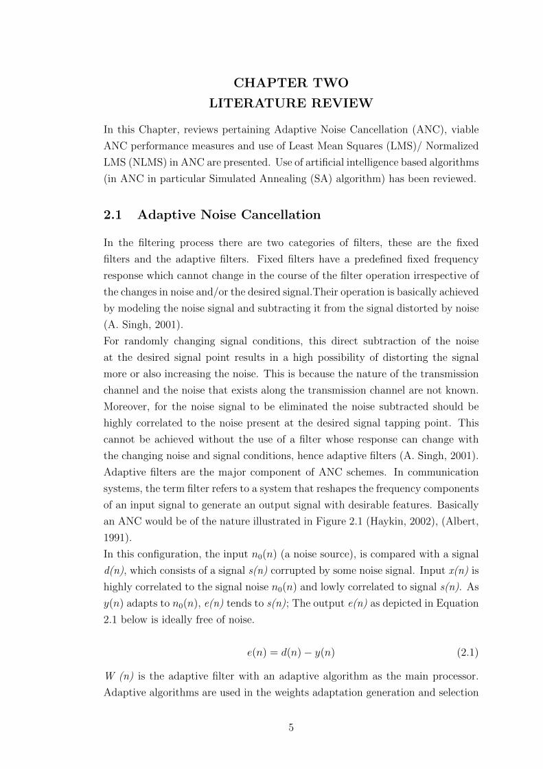
an ANC would be of the nature illustrated in Figure 2.1 (Haykin, 2002), (Albert,
1991).
In this configuration, the input n0(n) (a noise source), is compared with a signal
d(n), which consists of a signal s(n) corrupted by some noise signal. Input x(n) is
highly correlated to the signal noise n0(n) and lowly correlated to signal s(n). As
y(n) adapts to n0(n), e(n) tends to s(n); The output e(n) as depicted in Equation
2.1 below is ideally free of noise.
e(n) = d(n)− y(n) (2.1)
W (n) is the adaptive filter with an adaptive algorithm as the main processor.
Adaptive algorithms are used in the weights adaptation generation and selection
5
Figure 2.1: Adaptive noise canceller
to achieve the optimal weights thus, careful selection of the optimal adaptive filter
coefficients can lead to the error signal e (n) being equivalent to the signal s (n).
Applications of research in adaptive noise cancellation can be found in (Tsao et
al., 2018; Arif et al., 2017; Kapoor et al., 2017; Yelwande et al., 2017; D. Yang et
al., 2018).
2.2 Adaptive Noise cancellation performance measures
Adaptive noise cancellation performance measures can be categorized into: con-
vergence rate, computational complexity, robustness (Dimitris & Tsitsiklls, 1993)
and tracking capability (Widrow, 1975). In this thesis, performance measures of
interest are convergence rate and computational complexity, the subject of the
next two subsections. Convergence rate is a crucial factor in real-time systems.
Computational complexity is a factor of consideration in processors bearing low
computational power (typical of embedded systems).
2.2.1 Convergence rate
The convergence rate is the rate (time-wise) at which a filter converges to the
corresponding optimal state (minimal error state) (Haykin, 2002). Fast conver-
gence rate which is a time to converge issue, whilst ensuring stability, is a desired
characteristic of an adaptive system. During algorithm execution the error indica-
tors are evaluated and if they meet a predefined accuracy criterion the algorithm
execution stops (fast convergence implies low algorithm execution time).
6
2.2.2 Computational complexity
Computational complexity is of significance in real-time adaptive filter applica-
tions. In the implementation of a real time system, there are hardware limitations
that may affect the performance of the resultant system (Hameed, 2012). The
level of computational complexity in ANC is dependent on the algorithm em-
ployed in the weights adaptation process. Additionally, it is determined by the
number of multiplications, additions, subtractions and divisions during the algo-
rithm execution.
The higher the number of mathematical operations the more the complexity of the
algorithm (Bajic, 2005). A highly complex algorithm will require much greater
hardware and processing resources than a less complex algorithm.
The filter length (count of tap weights) of an adaptive system is inherently tied to
many of the other performance measures, particularly computational complexity.
The length of the filter specifies how accurately a given system can be modeled
by the adaptive filter. In addition, the filter length affects the convergence rate,
by increasing or decreasing computation time and complexity (Busetti, 2005).
Computation time and complexity are directly proportional to the filter length.
2.3 Adaptive noise cancellation solutions in literature
2.3.1 Use of LMS and NLMS algorithms
LMS and NLMS algorithms are commonly used in adaptive noise cancellation.
LMS algorithm minimizes the Mean Square Error (MSE) function given by Equa-
tion 2.2 iteratively by updating filter weights in a manner negative to the direction
of the gradient of the MSE function J(n).
J(n) = E|e(n)|2 (2.2)
where J (n) is the MSE function, E is the expectation operator, e (n) is the error
signal.
The weights adaptation process is as per Equation 2.3.
w(n+ 1) = w(n) + 0.5µ[−∇J(n)] (2.3)
where w is the filter weights vector, µ is the step-size, ∇J(n) is the gradient of
the MSE function.
In Equation 2.3, w corresponds to the filter weighting at a given point in time.
The constant µ (step-size) determines the time to converge as well as the stability
7
of the algorithm (Haykin, 2002). If the step size is made too small, the algorithm
will take more time to converge. However, if µ is made too large the convergence
rate is increased as well as the asymptotic error. Thus the selection of the step
size is a trade off between the application requirements, stability, accuracy and
convergence rate.
A subclass of LMS algorithms that is very commonly used is called the Normal-
ized Least Mean Square (NLMS) algorithm (Shi et al., 2019). This algorithm is
an upgrade to the standard LMS algorithm, and it is intended to increase con-
vergence speed, and stability of the algorithms despite increased complexity. The
reason for its development is the dependence of standard LMS adaptive filters
on the step size µ. The trade-offs regarding the step size can have a profound
impact on the applications. Increasing µ increases convergence speed, as well
as the asymptotic error, and hence decreases stability. For that reason, a scal-
ing factor for µ is added in order to constantly scale the step size, and in doing
so to increase the algorithm’s performance while increasing the stability. This
is achieved by normalizing the step size µ with an estimate of the input signal
power. The normalization factor, however, is inversely proportional to the sig-
nal instantaneous power (Shi et al., 2019). So, when the input signal is weak,
it increases the step size proportionally, and when the input is large, it reduces
the step size accordingly. It acts to both increase the stability, and increase the
convergence speed by allowing for variable step size to be used.(Widrow, 1975)
The definition of LMS algorithm can be presented as per Equations 2.4 through
2.6.
y(n) = wH(n)x(n) (2.4)
e(n) = d(n)− y(n) (2.5)
w(n+ 1) = w(n) + µe∗(n)x(n) (2.6)
where x(n) is the tap input vector and d(n) is the noise contaminated signal
s(n) + n0(n).
Normalized Least Mean Squares (NLMS) algorithm follows Equations 2.4 and
2.5, with a modification to the tap weight adaptation scheme as per Equation
2.7.
w(n+ 1) = w(n) +µe∗(n)x(n)
ε+ xH(n)x(n)(2.7)
8
where in equation 2.7, ε is a regularization parameter to avoid division by zero.
In Bajic (2005), research on use of normalized LMS algorithm and wavelet trans-
form domain LMS (WLMS) algorithm in ANC is carried out. Experimentation
with audio (music) signals is carried out. Convergence speed is used as the per-
formance measure, with the WLMS algorithm achieving higher convergence rates
than LMS attributed to reducing the cost of mathematical operations. However,
more research needs to be done for non speech signals on algorithms that would
lead to improved convergence speed.
In Hameed (2012), use of Least Mean Squares (LMS), Normalized Least Mean
Squares (NLMS) and Recursive Least Squares (RLS) algorithms in ANC is sim-
ulated using Matlab under a variety of conditions. An experimental implemen-
tation of the same is also done. Mean Square Error (MSE) is used as a measure
of noise reduction. Achieved convergence rates however need to be compared to
those of better performing AI based algorithms.
In G. Singh et al. (2013), design of an adaptive noise canceller for music signals
encountering colored noise using LMS algorithm is carried out successfully. Im-
proved SINR performance is observed. Use of AI algorithms in such filters need
to be studied since AI based algorithms promise better performance in terms of
convergence rates and solution accuracy.
In A. Singh (2001), various applications of the ANC are studied including an
in depth quantitative analysis of its use in canceling sinusoidal interferences as a
notch filter, for bias or low-frequency drift removal and as adaptive line enhancer.
Other applications dealt qualitatively are use of ANC without a reference input
for canceling periodic interference, adaptive self-tuning filter and cancellation
of noise in speech signals. Computer simulations for all cases are carried out
using Matlab software and experimental results are presented that illustrate the
usefulness of Adaptive Noise Canceling Technique.
2.3.2 Use of artificial intelligence algorithms
In Jatoth (2006), a bio-medical application of adaptive noise cancelling tech-
niques for filtering of obtained noisy Electro Cardio Gram signals using Genetic
Algorithm (GA) and Particle Swarm Optimization (PSO) algorithm is studied.
In addition, their performance in this application are compared to that of LMS.
The results of this study show that the two Artificial Intelligence (AI) algorithms
outweigh LMS in the solution accuracy. This study also gives an insight into
the use of AI in adaptive filters thus showing the possibility of use of Simulated
Annealing in adaptive noise cancellation.
9

In Zhou and Shao (2014), an improvement of Evolutionary Digital Filtering
(EDF) is presented. EDF notably exhibits the advantage of avoiding local op-
timums by utilizing cloning and mating rules in an adaptive noise cancellation
system. However, it is notable that convergence performance is hampered by
the large population of individuals required and the limited flow of information
communication among them. A beehive structure somewhat enables individu-
als on neighbour beehive nodes to easily pass information to each other and thus
enhances the information flow and search ability of the algorithm. Through intro-
duction of the beehive pattern evolutionary rules into the original EDF, this paper
overcomes the shortcomings of the original EDF. Simulation results demonstrate
the improved performance of the proposed algorithm in terms of convergence
speed compared with the conventional EDF. The results also verify the effec-
tiveness of the proposed algorithm in significantly extracting noise contaminated
signals.
In Thakur et al. (2014), an improved method based on evolutionary search meth-
ods is applied in speech signal de-noising. In Thakur et al. (2014), Artificial Bee
Colony (ABC), Cuckoo Search (CS) and Particle Swarm Optimization (PSO)
algorithms are utilized in adapting the filter parameters required for optimum
performance. Through simulations in Matlab, it is found that the ABC algo-
rithm and Cuckoo Search algorithm give better performance in terms of achieved
Signal-to-Noise Ratio (SNR) as compared to the PSO approach. The quantita-
tive (SNR, MSE and Maximum Error (ME)) and visual (de-noised speech signals)
results illustrate the superiority of the proposed technique over the conventional
speech signal de-noising techniques.
In Martinek et al. (2015), the implementation of Adaptive Neuro Fuzzy Inference
System (ANFIS) in non-linear suppression of noise and interference is presented.
The authors present a comprehensive ANFIS based system for adaptive interfer-
ence suppression in an audio communication link. The designed system is tested
on real voice signals. Performance measures utilized are Segmental Signal to
Noise Ratio (SSNR) and Dynamic Time Warping (DTW). The results obtained
imply that the ANFIS system is superior to LMS and Recursive Least Squares
(RLS) approaches.
Other studies involving application of artificial intelligence in adaptive noise can-
cellation can be found in (Pitchaiah et al., 2015; Shiva et al., 2016; Munjuluri et
al., 2015; Shubhra & Deepak, 2014; Ludger, 2015).
10
2.4 Simulated Annealing algorithm
2.4.1 Introduction
Simulated annealing (SA) algorithm is an optimization technique based on the
way in which a metal cools and freezes into a minimum energy crystalline struc-
ture (the annealing process). This algorithm was proposed in 1983 by Kirk et
al (Patrick et al., 1983) as a probabilistic method for finding global minima or
maxima of a cost function that may possess several local minima or maxima. A
description of the SA algorithm can be found in (Emile et al., 2014). An imple-
mentation of SA algorithm in hardware is described in (Ferreiro et al., 2013). A
classic optimization problem involving train scheduling is solved on the basis of
the SA algorithm in (Kang & Zhu, 2016).
2.4.2 Algorithm operation
SA algorithm approaches optimization problems in an analogous manner to a
bouncing ball approach (a ball bouncing over mountains (function crests) and
from valley (function troughs) to valley). It begins at a high ”temperature”
which enables the ball to make very high bounces (enables it to bounce over
any mountain to access any valley, given enough bounces). As the temperature
declines the ball cannot bounce so high and it can also settle to become trapped
in relatively small ranges of valleys (Yao, 2008).
In this algorithm, a random distribution of possible valleys or states of the system
to be explored is initially generated within the confines of some search region. An
acceptance distribution is also defined, which depends on the difference between
the function value of the present generated valley to be explored and the last
saved lowest valley. The acceptance distribution decides probabilistically whether
to stay in a new lower valley or to bounce out of it. All the generating and
acceptance distributions depend on the temperature. It has been proved that by
carefully controlling the rate of cooling of the temperature, SA can easily find the
global optimum (Garcia et al., 2012).
Solutions inferior to “current” solutions are accepted with a probability P given
in Equation 2.8, where δf is the increase in f (objective function value) and T is
a control parameter, which by analogy with the original application is known as
the system “temperature” (Patrick et al., 1983).
P =1
eδf/T(2.8)
11
2.4.3 Operational elements
The basic operational elements of the SA algorithm are:
� A representation of possible solutions.
� A generator of random changes in solutions.
� A means of evaluating the problem functions.
� An annealing schedule which is an initial temperature and rules for lowering
it as the search progresses.
Figure 2.2 shows the SA algorithm flowchart (Busetti, 2005). Initially, when the
annealing “temperature” is high, some large increases in the objective function f
are accepted and some areas far from the optimum are explored. As execution
continues and temperature T decreases as per the cooling schedule, fewer uphill
excursions are tolerated (and those that are tolerated are of smaller magnitude).
The main equation corresponds to the probability of accepting a worse state and
is given by Equation 2.9.
P =1
ec/t(2.9)
where: P is the probability of accepting a worse state (a worse state is accepted
if P is greater than a random number between 0 and 1.), c is the raw change in
the evaluation function, t is the current “temperature”.
This probability function is borrowed from Boltzmann law of thermodynamics.
The law of thermodynamics states that for some physical body at temperature, t,
the probability P of an increase in energy magnitude δE, is as given in Equation
2.10 where k is the Boltzmann’s constant.
P (δE) =1
eδE/kt(2.10)
Temperature reduction involves a linear decrement as given in Equation 2.11.
ti = αti−1 (2.11)
where α is a positive constant less than 1 i.e 0 < α < 1.
2.4.4 One Dimensional Minimization problem
A simple one-dimensional minimization problem is depicted in Figure 2.3. The
minimal value is as indicated by an asterisk. This minimal value is to be obtained
12

Input and assess initial solution
Estimate initial temperature
Generate new solution
Assess new solution
Accept new solution
Update stores
Adjust temperature
Terminate search
Stop
Yes
Yes
No
No
Figure 2.2: SA algorithm operation
through the SA algorithm.
Figure 2.3: Typical one-dimension minimization problem
13
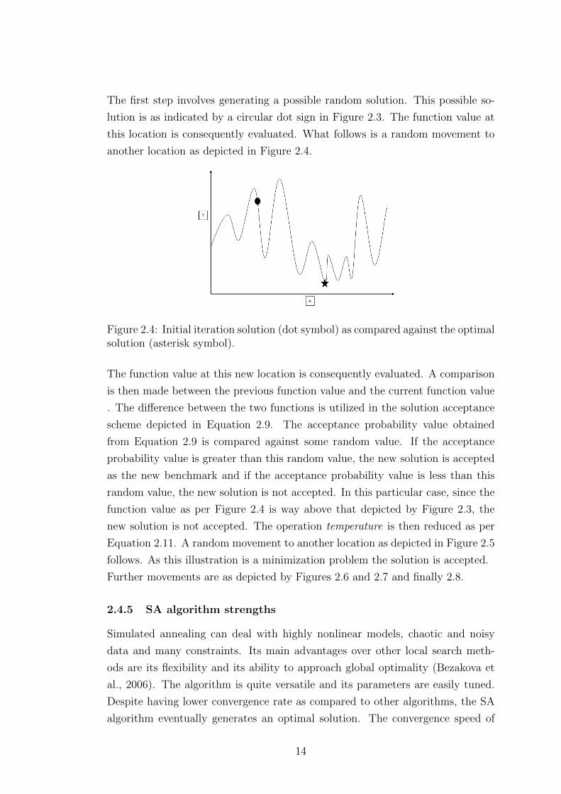
The first step involves generating a possible random solution. This possible so-
lution is as indicated by a circular dot sign in Figure 2.3. The function value at
this location is consequently evaluated. What follows is a random movement to
another location as depicted in Figure 2.4.
Figure 2.4: Initial iteration solution (dot symbol) as compared against the optimalsolution (asterisk symbol).
The function value at this new location is consequently evaluated. A comparison
is then made between the previous function value and the current function value
. The difference between the two functions is utilized in the solution acceptance
scheme depicted in Equation 2.9. The acceptance probability value obtained
from Equation 2.9 is compared against some random value. If the acceptance
probability value is greater than this random value, the new solution is accepted
as the new benchmark and if the acceptance probability value is less than this
random value, the new solution is not accepted. In this particular case, since the
function value as per Figure 2.4 is way above that depicted by Figure 2.3, the
new solution is not accepted. The operation temperature is then reduced as per
Equation 2.11. A random movement to another location as depicted in Figure 2.5
follows. As this illustration is a minimization problem the solution is accepted.
Further movements are as depicted by Figures 2.6 and 2.7 and finally 2.8.
2.4.5 SA algorithm strengths
Simulated annealing can deal with highly nonlinear models, chaotic and noisy
data and many constraints. Its main advantages over other local search meth-
ods are its flexibility and its ability to approach global optimality (Bezakova et
al., 2006). The algorithm is quite versatile and its parameters are easily tuned.
Despite having lower convergence rate as compared to other algorithms, the SA
algorithm eventually generates an optimal solution. The convergence speed of
14
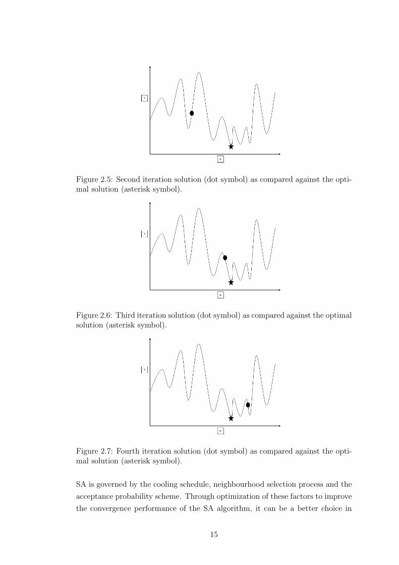
Figure 2.5: Second iteration solution (dot symbol) as compared against the opti-mal solution (asterisk symbol).
Figure 2.6: Third iteration solution (dot symbol) as compared against the optimalsolution (asterisk symbol).
Figure 2.7: Fourth iteration solution (dot symbol) as compared against the opti-mal solution (asterisk symbol).
SA is governed by the cooling schedule, neighbourhood selection process and the
acceptance probability scheme. Through optimization of these factors to improve
the convergence performance of the SA algorithm, it can be a better choice in
15
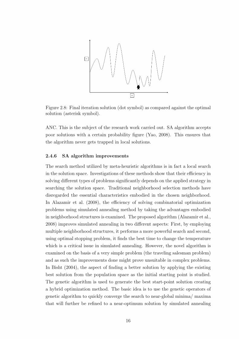
Figure 2.8: Final iteration solution (dot symbol) as compared against the optimalsolution (asterisk symbol).
ANC. This is the subject of the research work carried out. SA algorithm accepts
poor solutions with a certain probability figure (Yao, 2008). This ensures that
the algorithm never gets trapped in local solutions.
2.4.6 SA algorithm improvements
The search method utilized by meta-heuristic algorithms is in fact a local search
in the solution space. Investigations of these methods show that their efficiency in
solving different types of problems significantly depends on the applied strategy in
searching the solution space. Traditional neighborhood selection methods have
disregarded the essential characteristics embodied in the chosen neighborhood.
In Alazamir et al. (2008), the efficiency of solving combinatorial optimization
problems using simulated annealing method by taking the advantages embodied
in neighborhood structures is examined. The proposed algorithm (Alazamir et al.,
2008) improves simulated annealing in two different aspects: First, by employing
multiple neighborhood structures, it performs a more powerful search and second,
using optimal stopping problem, it finds the best time to change the temperature
which is a critical issue in simulated annealing. However, the novel algorithm is
examined on the basis of a very simple problem (the traveling salesman problem)
and as such the improvements done might prove unsuitable in complex problems.
In Bisht (2004), the aspect of finding a better solution by applying the existing
best solution from the population space as the initial starting point is studied.
The genetic algorithm is used to generate the best start-point solution creating
a hybrid optimization method. The basic idea is to use the genetic operators of
genetic algorithm to quickly converge the search to near-global minima/ maxima
that will further be refined to a near-optimum solution by simulated annealing
16
algorithm. The new hybrid algorithm has been applied to optimal weapon allo-
cation in multilayer defense scenario problem to arrive at a better solution than
produced by simulated annealing algorithm alone. However, algorithm hybridiza-
tion leads to more computationally complex algorithms and consequently longer
convergence time.
In Bayram and Azahin (2013), a study on improving the search capability of SA
algorithm through integration of two new neighborhood mechanisms is presented.
The results derived on the basis of the Travelling Salesman Problem have shown
that the proposed techniques are more effective than conventional SA, both in
terms of solution quality and time. However, the improvement done has not
been studied on the basis of any other optimization problem. The proposed
integration mechanism potentially leads to an increase in computation complexity,
a negativity in terms of convergence time.
In Bezakova et al. (2006), an improved cooling schedule for simulated annealing
algorithms for combinatorial counting problems is presented. Under the new
schedule the rate of cooling accelerates as the temperature decreases. Thus,
fewer intermediate temperatures are needed as the simulated annealing algorithm
moves from the high temperature (easy region) to the low temperature (difficult
region). This results in accelerated algorithm execution speed. However, the
proposed approach has the potential of hampering on solution accuracy.
In Y. Li et al. (2013), a hybrid Genetic algorithm/ SA algorithm is proposed and
applied successfully in an e-supply chain problem. Another scenario featuring
algorithm hybridization can be found in (Yannibelli & Amandi, 2013), whereby
the SA algorithm is hybridized with evolutionary search algorithm in a scheduling
problem yielding good results. In Nouri et al. (2013), a hybrid firefly-SA algorithm
is developed for a shop problem with learning features and flexible maintenance
activities yielding significant results. All in all, algorithm hybridization usually
results in computation complexity and reduction of speed of convergence.
Other SA algorithm improvements can be found in (Zhang et al., 2017; Xu et al.,
2017; Wu et al., 2017; Shang et al., 2020).
2.4.7 SA Versus Other AI Algorithms
SA’s major advantage over other non-gradient based methods (such as Genetic
Algorithm, Tabu Search algorithm, Differential Evolution) is an ability to avoid
becoming trapped in local minima. This is because the algorithm employs a ran-
dom search technique, which not only accepts changes that decrease the objective
function value f (assuming a minimization problem), but also some changes that
17
increase it with some degree of probability. This therefore guarantees that SA per-
forms better than other AI algorithms (such as Genetic Algorithm, Tabu Search
algorithm, Differential Evolution) in optimization problems thus the choice in
ANC, the subject of this research. However, the major drawback of SA is slow
execution speed which can be increased by optimization of the control parame-
ters, acceptance probability and the cooling schedule.This is the key focus of this
research.
2.5 Summary
This chapter has reviewed pertinent issues in ANC. ANC performance measures
in particular convergence rate and computation complexity have been reviewed.
A review on the use of LMS/ NLMS in ANC has been presented. This is along-
side use of artificial intelligence based algorithms in ANC in particular the SA
algorithm. Various applications of SA algorithm in ANC have been presented.
The shortcomings of the SA algorithm have been presented alongside a review of
potential improvements.
It has been noted that the convergence speed of SA is mainly governed by the
cooling schedule and the utilized acceptance probability scheme. Through op-
timization of these two factors to improve the convergence performance of the
SA algorithm, it can be a better choice in ANC. Corresponding SA algorithm
improvements are presented in Chapter 3 of this Thesis.
It is desirable that the improvements made on the SA algorithm are analyzed on
the basis of different signals and noise conditions, a task carried out in Chapter
4 of this Thesis.
In the next Chapter, an ANC simulation model is developed. The development of
an improved SA algorithm (through improved acceptance probability and cooling
schedule) is also presented.
18

CHAPTER THREE
METHODOLOGY
In this chapter an adaptive noise cancellation model is developed. Three signal
formats (electrocardiogram, sinusoidal and irregular random signals) utilized in
the subsequent chapter are presented. Euclidean distance and correlation coeffi-
cient performance measures have been presented.
Improvements on the conventional SA algorithm performance by proposed cooling
schedule and acceptance probability schemes have been presented.
The procedural steps taken towards the application of the standard SA algorithm
and its modified version in adaptive noise cancellation have been presented. This
is alongside a highlight of the methods applied in establishing the effectiveness of
the standard and modified Simulated Annealing algorithm in ANC in comparison
to standard LMS and NLMS algorithms.
3.1 Development of an adaptive noise cancellation model
3.1.1 ANC model formulation
An adaptive noise canceller is illustrated in Figure 2.1.
To observe the outcome of adaptive noise cancellation in a broad way, a series
of signals are used as input signal S. The signals utilized are Electrocardiogram
signals, sinusoidal signals and randomly generated signals. Additive White Gaus-
sian Noise (AWGN) plus other random noise is used as the noise data n0. AWGN
is representative of naturally occurring noise. A viable filter order is identified
in line with the problem at hand (long enough to allow for proper performance
bearing in mind the higher the order, the higher the computation intensity).
3.1.2 Cost function formulation
As per Figure 2.1, an adaptive noise canceller has two inputs primary (repre-
sented by d) and reference (represented by x). The primary input is a signal s
that is corrupted by the presence of noise n0 that is uncorrelated with the signal.
The reference input is a noise signal x(n) that is uncorrelated with the signal s
but correlated in some way with the noise n0. The noise x(n) passes through
an adaptive filter to generate an output y that is a close estimate of the primary
input noise n0. This noise estimate is consequently subtracted from the corrupted
signal to generate an estimate of the signal e, the ANC system output.
In typical noise cancellation systems, the objective is usually to produce a system
output (Equation 3.12) that is a best fit in the least squares sense to the signal
19
of interest s. This objective is met through feeding back the system output e
to the adaptive filter and consequently adjusting the filter through an adaptive
algorithm with an aim of minimizing the total system output power. The system
output is typically the error signal for the adaptive process.
In the following analysis, it is assumed that s, n0 and n1 are statistically stationary
and have zero means; The signal s is uncorrelated with n0 and n1, and n1 is
correlated with n0.
e = s+ n0 − y (3.12)
e2 = s2 + (n0 − y)2 + 2s(n0 − y) (3.13)
Taking the expectation of both sides in Equation 3.13 and realizing that s is
uncorrelated with n0 and y,
E[e2] = E[s2] + E[(n0 − y)2] + 2E[s(n0 − y)] (3.14)
and consequently
E[e2] = E[s2] + E[(n0 − y)2] (3.15)
The signal power E[s2] is not affected since the filter is adjusted to minimize the
total output power E[e2] as per Equation 3.16.
minE[e2] = E[s2] +minE[(n0 − y)2] (3.16)
When the filter weights are adjusted with an aim towards minimizing the total
output power E[e2], the output noise power E[(n0 − y)2 is also minimized. Since
the signal power in the output remains constant, minimizing the total output
power maximizes the output Signal to Noise Ratio (SNR).
In consideration of the various signal formats described in the previous section,
the cost function developed is as per Equation 3.17.
ES = NCS −WNE (3.17)
where: ES denotes Error Signal, NCS denotes Noise Contaminated Signal, WNE
denotes Weighted Noise Estimate.
Let wT be some MX1 tap-weight vector, wT = [w1, w2, ..., wM ] where M is the
filter length.
Let xT (n) be some MX1 input vector, xT (n) = [x(n), x(n−1), ..., x(n−M + 1)].
20
Then the filter output y(n|xn) can be framed as wHx(n) where H is the Hermitian
transpose operator.
Equation 3.17 can consequently be written as per Equation 3.18, where e(n) is
the filter output, d(n) the noise contaminated signal, w(n) a set of filter weights
and x(n) an estimate of the noise signal.
e(n) = d(n)−wHx(n) (3.18)
The mean squared error (cost function) J(w) can consequently be expressed as
E[e(n)e*(n)] (expanded in Equation 3.19).
J(w) = E[(d(n)−wHx(n))(d∗(n)− xH(n)w)] (3.19)
Minimizing the cost function as per Equation 3.19 through filter weights opti-
mization yields an optimal solution (ideally a noise free signal).
3.1.3 Correlation performance measure
In general, the term correlation can imply any statistical association, though it
commonly refers to how close two variables are in terms of a linear relationship
with each other.
Pearson’s product-moment correlation coefficient
“Pearson product-moment correlation coefficient”, or “Pearson’s correlation co-
efficient”, commonly referred to as “correlation coefficient” is a common measure
of dependence between two variables. Pearson’s correlation coefficient is obtained
by dividing the covariance of the two variables under consideration by the product
of their standard deviations.
The population correlation coefficient ρX,Y between two random variables X and
Y with expected values µX and µY and standard deviations σX and σY is defined
as per Equation 3.20 below.
ρX,Y = corr(X, Y ) =cov(X, Y )
σXσY=E[(X − µX)(Y − µY )]
σXσY(3.20)
In Equation 3.20:
E is the expectation operator;
cov implies covariance;
corr implies correlation coefficient.
The Pearson correlation measure is defined/ valid if and only if both variables’
standard deviations are non-zero and finite. The Pearson correlation measure is
+1 in the case of a perfect direct (increasing) linear relationship (correlation). The
21
Pearson correlation measure is -1 in the case of a perfect decreasing (inverse) linear
relationship (anti-correlation). In all other cases, the Pearson correlation measure
is a value within the interval (-1, 1). As the correlation measure approaches
zero, there is less of a relationship between the variables in question (closer to
uncorrelated). A coefficient with a value close to either -1 or 1 implies strong
correlation between variables.
3.1.4 Euclidean distance performance measure
In the performance evaluation comparison, Euclidean distances play a pivotal role
in the analysis of final solution convergence for different optimization algorithms
studied in this thesis. Euclidean distance is a measure of similarity or dissimilarity
that can be used to compare two sets of vectors and compute a single number
which evaluates the similarity/dissimilarity. For two points in a two dimensional
space Euclidean distance is the length of the path connecting them in the plane.
The distance between say two points (x1, y1) and (x2, y2, ) is given by Equation
3.21.
d =√
(x2 − x1)2 + (y2 − y1)2. (3.21)
In Euclidean three-space plane, the distance between points (x1, y1, z1) and (x2, y2, z2)
is given by Equation 3.22.
d =√
(x2 − x1)2 + (y2 − y1)2 + (z2 − z1)2. (3.22)
In general, given two n-dimensional vectors:
� x = [x1, x2, x3 ... xn]T
� y = [y1, y2, y3 ... yn]T
The Euclidian distance d between them is given by Equation 3.23.
d =
√√√√ n∑i=1
(xi − yi)2 (3.23)
3.2 Simulated annealing algorithm improvement
The structure of the utilized standard SA algorithm is of the nature described in
the listing below (implemented in MATLAB).
22
1. The SA function definition is framed as: [OptimalPosition,OptimalValue]
= SA(CostFunction, InitialRandomSolution, SAoptions).
The SAoptions structure holds the following parameters:
� cooling schedule; formulated as a linear relationship: CurrentTemper-
ature=PreviousTemperature*0.8.
� initial temperature; formulated as 1
� solution generation; a small random modification of the current solu-
tion; formulated as: NewSolution= CurrentSolution+SmallRandomValue.
2. Evaluation of the cost function at the initial random solution position.
3. Generation of a new solution position as per the solution generation mech-
anism described in 1.
4. Evaluation of the cost function at the new solution position. If the eval-
uation yields a better result than the previous result, the current solution
position is adopted. If the evaluation yields a worse result than the previous
result, the current solution position is adopted with some probability value
defined as a check on: RandomV alue < exp(PreviousResult−CurrentResult)
(Temperature) .
5. Temperature is consequently adjusted as per the cooling schedule defined
in 1.
6. Steps 3 to 5 are repeated until some stopping criteria is met.
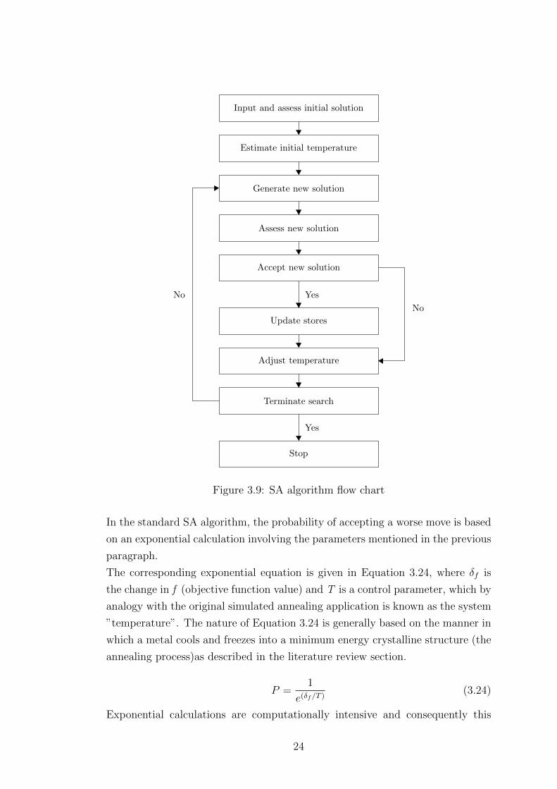
Figure 3.9 illustrates the SA algorithm flow chart.
As seen from the above structure, the solution acceptance scheme and the cooling
schedule play a pivotal role in the SA algorithm. The improvements done on the
SA algorithm focus on the two items, and are consequently described.
3.2.1 Acceptance Probability
During SA algorithm run, not only better solutions are accepted but also worse
solutions but with a decreasing probability as execution progresses. The aim of
accepting worse solutions during SA algorithm run is to avoid convergence to
a local minimum. The probability of accepting a worse solution is determined
by two parameters: the temperature and the difference between the objective
function values of current solution and neighbor solution (solution under probe).
23
Input and assess initial solution
Estimate initial temperature
Generate new solution
Assess new solution
Accept new solution
Update stores
Adjust temperature
Terminate search
Stop
Yes
Yes
No
No
Figure 3.9: SA algorithm flow chart
In the standard SA algorithm, the probability of accepting a worse move is based
on an exponential calculation involving the parameters mentioned in the previous
paragraph.
The corresponding exponential equation is given in Equation 3.24, where δf is
the change in f (objective function value) and T is a control parameter, which by
analogy with the original simulated annealing application is known as the system
”temperature”. The nature of Equation 3.24 is generally based on the manner in
which a metal cools and freezes into a minimum energy crystalline structure (the
annealing process)as described in the literature review section.
P =1
e(δf/T )(3.24)
Exponential calculations are computationally intensive and consequently this
24
slows down algorithm execution speed whilst taking up huge processing resources.
Use of simpler but efficient functions would result in increased algorithm conver-
gence rate.
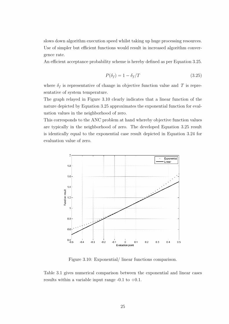
An efficient acceptance probability scheme is hereby defined as per Equation 3.25.
P (δf ) = 1− δf/T (3.25)
where δf is representative of change in objective function value and T is repre-
sentative of system temperature.
The graph relayed in Figure 3.10 clearly indicates that a linear function of the
nature depicted by Equation 3.25 approximates the exponential function for eval-
uation values in the neighborhood of zero.
This corresponds to the ANC problem at hand whereby objective function values
are typically in the neighborhood of zero. The developed Equation 3.25 result
is identically equal to the exponential case result depicted in Equation 3.24 for
evaluation value of zero.
Figure 3.10: Exponential/ linear functions comparison.
Table 3.1 gives numerical comparison between the exponential and linear cases
results within a variable input range -0.1 to +0.1.
25
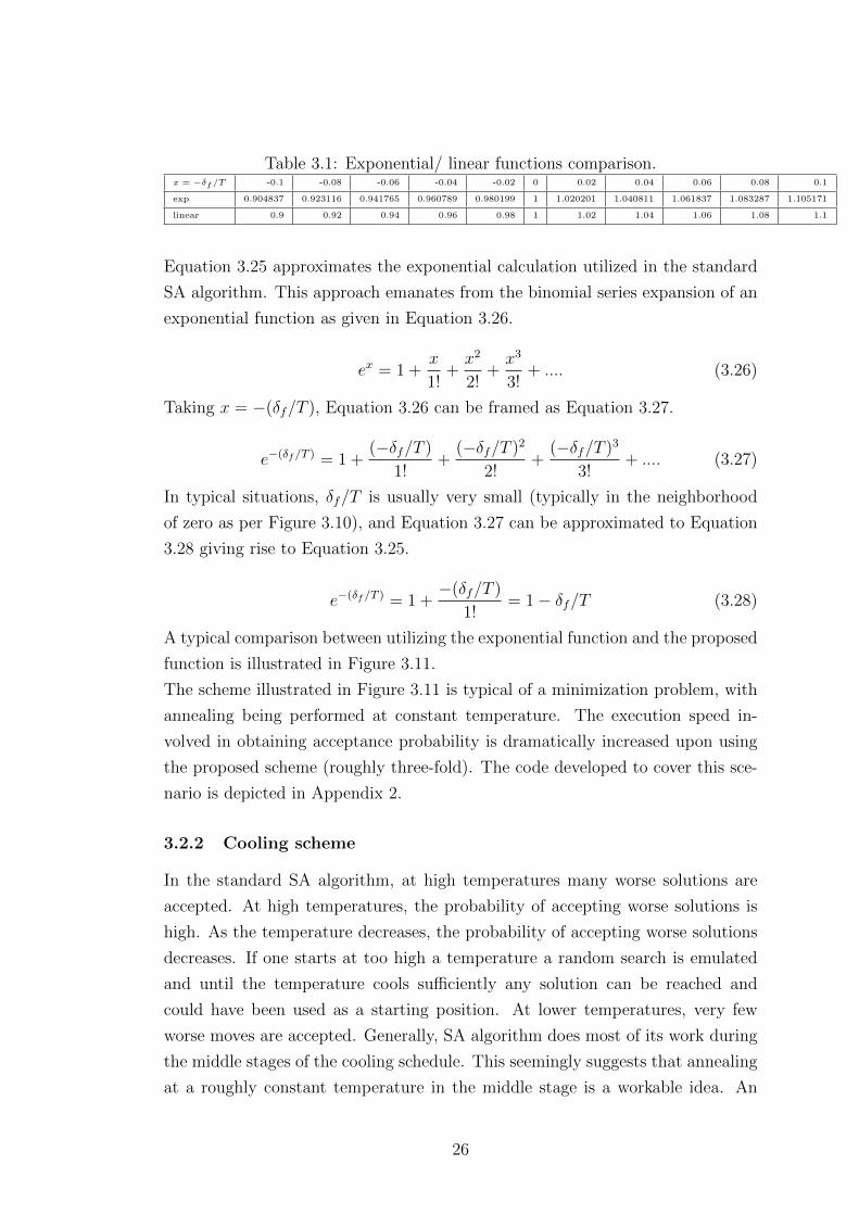
Table 3.1: Exponential/ linear functions comparison.x = −δf/T -0.1 -0.08 -0.06 -0.04 -0.02 0 0.02 0.04 0.06 0.08 0.1
exp 0.904837 0.923116 0.941765 0.960789 0.980199 1 1.020201 1.040811 1.061837 1.083287 1.105171
linear 0.9 0.92 0.94 0.96 0.98 1 1.02 1.04 1.06 1.08 1.1
Equation 3.25 approximates the exponential calculation utilized in the standard
SA algorithm. This approach emanates from the binomial series expansion of an
exponential function as given in Equation 3.26.
ex = 1 +x
1!+x2
2!+x3
3!+ .... (3.26)
Taking x = −(δf/T ), Equation 3.26 can be framed as Equation 3.27.
e−(δf/T ) = 1 +(−δf/T )
1!+
(−δf/T )2
2!+
(−δf/T )3
3!+ .... (3.27)
In typical situations, δf/T is usually very small (typically in the neighborhood
of zero as per Figure 3.10), and Equation 3.27 can be approximated to Equation
3.28 giving rise to Equation 3.25.
e−(δf/T ) = 1 +−(δf/T )
1!= 1− δf/T (3.28)
A typical comparison between utilizing the exponential function and the proposed
function is illustrated in Figure 3.11.
The scheme illustrated in Figure 3.11 is typical of a minimization problem, with
annealing being performed at constant temperature. The execution speed in-
volved in obtaining acceptance probability is dramatically increased upon using
the proposed scheme (roughly three-fold). The code developed to cover this sce-
nario is depicted in Appendix 2.
3.2.2 Cooling scheme
In the standard SA algorithm, at high temperatures many worse solutions are
accepted. At high temperatures, the probability of accepting worse solutions is
high. As the temperature decreases, the probability of accepting worse solutions
decreases. If one starts at too high a temperature a random search is emulated
and until the temperature cools sufficiently any solution can be reached and
could have been used as a starting position. At lower temperatures, very few
worse moves are accepted. Generally, SA algorithm does most of its work during
the middle stages of the cooling schedule. This seemingly suggests that annealing
at a roughly constant temperature in the middle stage is a workable idea. An
26
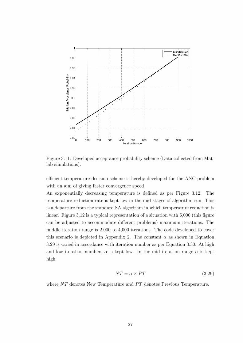
Figure 3.11: Developed acceptance probability scheme (Data collected from Mat-lab simulations).
efficient temperature decision scheme is hereby developed for the ANC problem
with an aim of giving faster convergence speed.
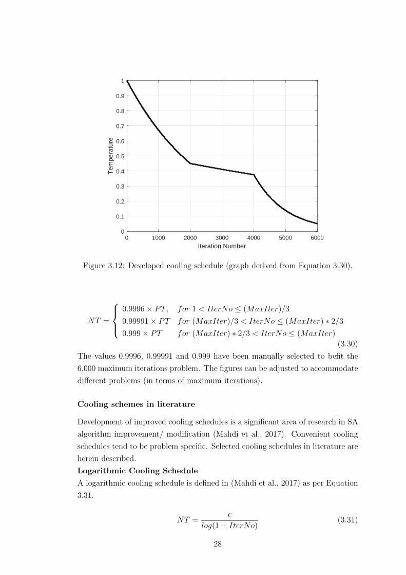
An exponentially decreasing temperature is defined as per Figure 3.12. The
temperature reduction rate is kept low in the mid stages of algorithm run. This
is a departure from the standard SA algorithm in which temperature reduction is
linear. Figure 3.12 is a typical representation of a situation with 6,000 (this figure
can be adjusted to accommodate different problems) maximum iterations. The
middle iteration range is 2,000 to 4,000 iterations. The code developed to cover
this scenario is depicted in Appendix 2. The constant α as shown in Equation
3.29 is varied in accordance with iteration number as per Equation 3.30. At high
and low iteration numbers α is kept low. In the mid iteration range α is kept
high.
NT = α× PT (3.29)
where NT denotes New Temperature and PT denotes Previous Temperature.
27
0 1000 2000 3000 4000 5000 6000
Iteration Number
0
0.1
0.2
0.3
0.4
0.5
0.6
0.7
0.8
0.9
1
Tem
pera
ture
Figure 3.12: Developed cooling schedule (graph derived from Equation 3.30).
NT =
0.9996× PT, for 1 < IterNo ≤ (MaxIter)/3
0.99991× PT for (MaxIter)/3 < IterNo ≤ (MaxIter) ∗ 2/3
0.999× PT for (MaxIter) ∗ 2/3 < IterNo ≤ (MaxIter)
(3.30)
The values 0.9996, 0.99991 and 0.999 have been manually selected to befit the
6,000 maximum iterations problem. The figures can be adjusted to accommodate
different problems (in terms of maximum iterations).
Cooling schemes in literature
Development of improved cooling schedules is a significant area of research in SA
algorithm improvement/ modification (Mahdi et al., 2017). Convenient cooling
schedules tend to be problem specific. Selected cooling schedules in literature are
herein described.
Logarithmic Cooling Schedule
A logarithmic cooling schedule is defined in (Mahdi et al., 2017) as per Equation
3.31.
NT =c
log(1 + IterNo)(3.31)
28
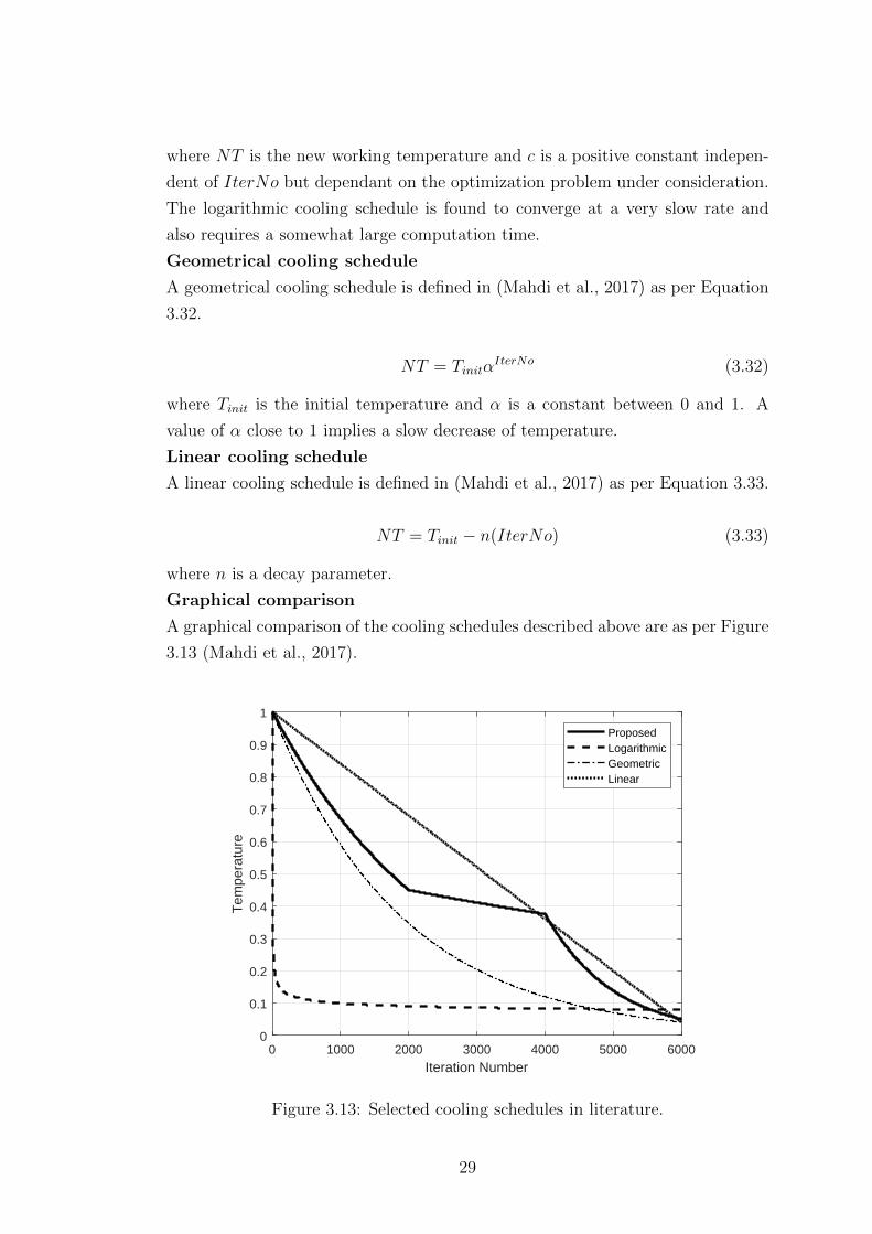
where NT is the new working temperature and c is a positive constant indepen-
dent of IterNo but dependant on the optimization problem under consideration.
The logarithmic cooling schedule is found to converge at a very slow rate and
also requires a somewhat large computation time.
Geometrical cooling schedule
A geometrical cooling schedule is defined in (Mahdi et al., 2017) as per Equation
3.32.
NT = TinitαIterNo (3.32)
where Tinit is the initial temperature and α is a constant between 0 and 1. A
value of α close to 1 implies a slow decrease of temperature.
Linear cooling schedule
A linear cooling schedule is defined in (Mahdi et al., 2017) as per Equation 3.33.
NT = Tinit − n(IterNo) (3.33)
where n is a decay parameter.
Graphical comparison
A graphical comparison of the cooling schedules described above are as per Figure
3.13 (Mahdi et al., 2017).
0 1000 2000 3000 4000 5000 6000
Iteration Number
0
0.1
0.2
0.3
0.4
0.5
0.6
0.7
0.8
0.9
1
Tem
pera
ture
ProposedLogarithmicGeometricLinear
Figure 3.13: Selected cooling schedules in literature.
29

The cooling schedule constants for the schemes illustrated in Figure 3.13 are given
in Table 3.2.
Table 3.2: Selected cooling schedules in literature: constant values used.
Cooling schedule Parameters
Proposed Adaptive, as per Equation 3.30
Logarithmic c=0.3
Geometric α = 0.99947
Linear n = 0.00016
The cooling schedule schemes’ computation time is given in Table 3.3. The val-
ues are generated through Matlab’s computation timer in a uniform computation
environment. Lower computation time is indicative of lower computation com-
plexity. The proposed cooling schedule performs than the other schedules.
Table 3.3: Selected cooling schedules in literature: computation time.
Cooling schedule Function evaluation time (seconds)
Proposed 0.0012
Logarithmic 0.0053
Geometric 0.0034
Linear 0.0027
3.3 Application and analysis of the modified SA algorithm
in adaptive noise cancellation
This section presents the procedural steps taken towards the application and
analysis of the modified SA algorithm in adaptive noise cancellation. Performance
validation is on the basis of a comparative analysis against the standard SA
algorithm. Signal formats utilized in the next Chapter (Results and Discussion)
have been brought to the fore.
3.3.1 Noise cancellation framework
In general, the cost function as per Equation 3.34 is utilized in the adaptive noise
cancellation process.
J(w) = E[(d(n)−wHx(n))(d∗(n)− xH(n)w)] (3.34)
30
Minimizing the cost function as per Equation 3.34 through filter weights opti-
mization yields an optimal solution (ideally a noise free signal). The modified
SA algorithm is utilized in obtaining the optimal weights. The performance of
the modified SA algorithm is to be weighed against that of the standard SA
algorithm.
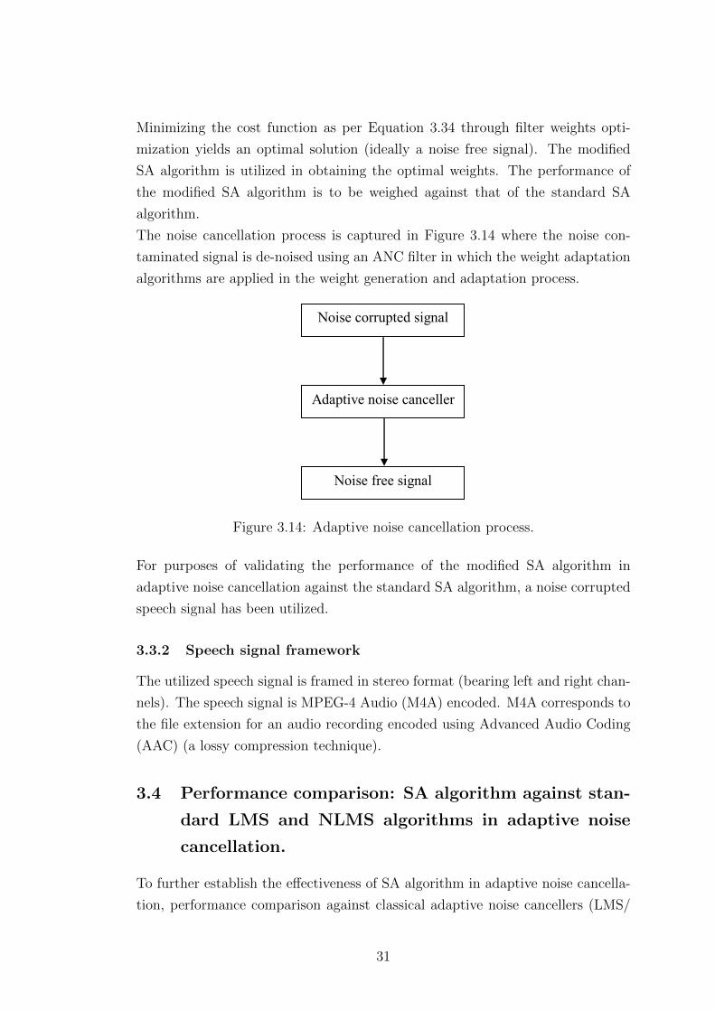
The noise cancellation process is captured in Figure 3.14 where the noise con-
taminated signal is de-noised using an ANC filter in which the weight adaptation
algorithms are applied in the weight generation and adaptation process.
Noise corrupted signal
Adaptive noise canceller
Noise free signal
Figure 3.14: Adaptive noise cancellation process.
For purposes of validating the performance of the modified SA algorithm in
adaptive noise cancellation against the standard SA algorithm, a noise corrupted
speech signal has been utilized.
3.3.2 Speech signal framework
The utilized speech signal is framed in stereo format (bearing left and right chan-
nels). The speech signal is MPEG-4 Audio (M4A) encoded. M4A corresponds to
the file extension for an audio recording encoded using Advanced Audio Coding
(AAC) (a lossy compression technique).
3.4 Performance comparison: SA algorithm against stan-
dard LMS and NLMS algorithms in adaptive noise
cancellation.
To further establish the effectiveness of SA algorithm in adaptive noise cancella-
tion, performance comparison against classical adaptive noise cancellers (LMS/
31
NLMS algorithm based) is done. The signal formats described in Section 3.4.1
have been utilized (Sinusoidal, irregular and fetal electrocardiogram signals).
3.4.1 Utilized signal formats
Electrocardiogram signals framework
Continuous monitoring of fetal heart condition during pregnancy is of great med-
ical significance. One area of application of adaptive noise cancellation is in ex-
traction of fetal heartbeat signals from signal measurements taken at the mother’s
abdomen. Electro Cardio Gram (ECG) is used to record changes in heartbeat
thus can diagnose any heart malfunction. The obtained fetal ECG (FECG) sig-
nal is usually severely contaminated by maternal cardiogram (MECG), and other
external interferences. The resultant low signal to noise ratio of fetal ECG makes
it difficult to analyze it effectively necessitating noise cancellation mechanisms.
Research involving application of adaptive noise cancellation in medical instru-
mentation can be found in (L. Li et al., 2016) in which lung sound noise cancel-
lation and classification is performed satisfactorily. Other corresponding appli-
cations can be found in (Abdelghani et al., 2015), (Dewangan & M., 2014) and
(Tanaka et al., 2016).
Typical waveforms corresponding to electrocardiogram signals for both the mother
and the corresponding fetus are hereby defined.
Mother’s heartbeat
The mother’s heart rate is simulated to be approximately 89 beats per minute
with the peak voltage of the signal being 3.25 millivolts. This is informed by the
work laid out in (Ghodsi et al., 2010). A typical mother’s heartbeat signal (noise
free) is as given in Figure 3.15.
32
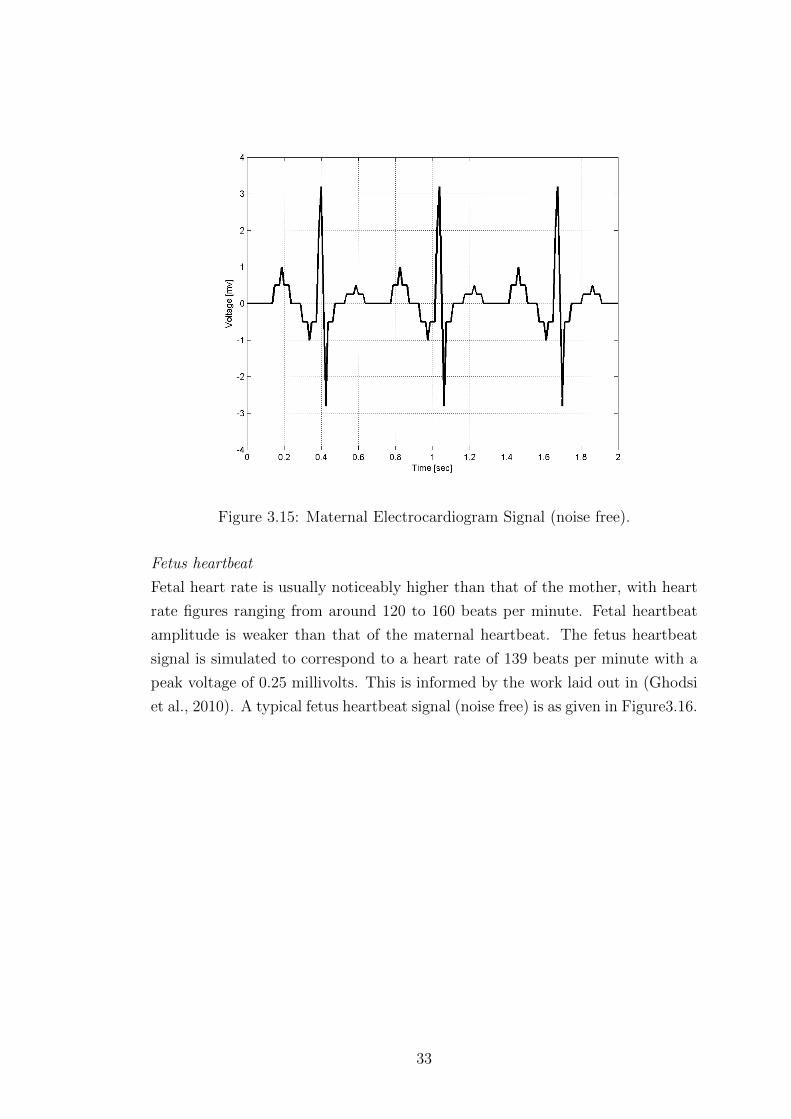
Figure 3.15: Maternal Electrocardiogram Signal (noise free).
Fetus heartbeat
Fetal heart rate is usually noticeably higher than that of the mother, with heart
rate figures ranging from around 120 to 160 beats per minute. Fetal heartbeat
amplitude is weaker than that of the maternal heartbeat. The fetus heartbeat
signal is simulated to correspond to a heart rate of 139 beats per minute with a
peak voltage of 0.25 millivolts. This is informed by the work laid out in (Ghodsi
et al., 2010). A typical fetus heartbeat signal (noise free) is as given in Figure3.16.
33
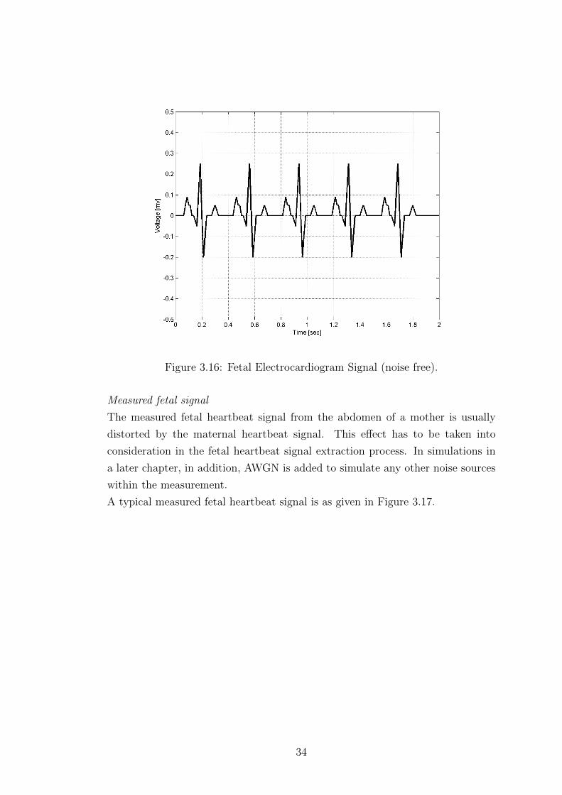
Figure 3.16: Fetal Electrocardiogram Signal (noise free).
Measured fetal signal
The measured fetal heartbeat signal from the abdomen of a mother is usually
distorted by the maternal heartbeat signal. This effect has to be taken into
consideration in the fetal heartbeat signal extraction process. In simulations in
a later chapter, in addition, AWGN is added to simulate any other noise sources
within the measurement.
A typical measured fetal heartbeat signal is as given in Figure 3.17.
34
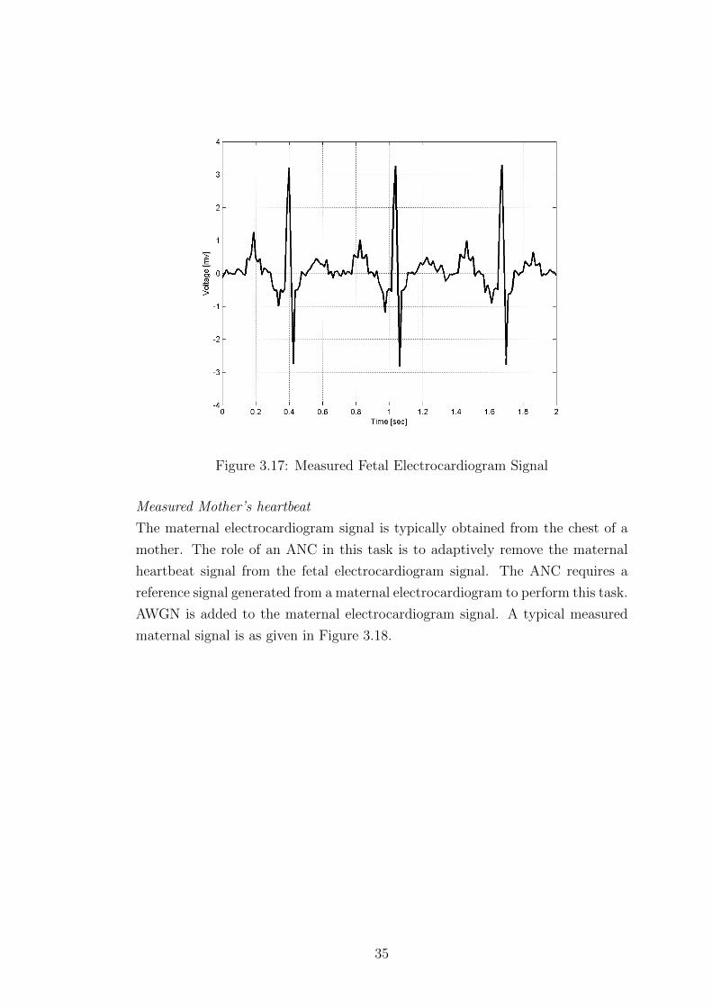
Figure 3.17: Measured Fetal Electrocardiogram Signal
Measured Mother’s heartbeat
The maternal electrocardiogram signal is typically obtained from the chest of a
mother. The role of an ANC in this task is to adaptively remove the maternal
heartbeat signal from the fetal electrocardiogram signal. The ANC requires a
reference signal generated from a maternal electrocardiogram to perform this task.
AWGN is added to the maternal electrocardiogram signal. A typical measured
maternal signal is as given in Figure 3.18.
35
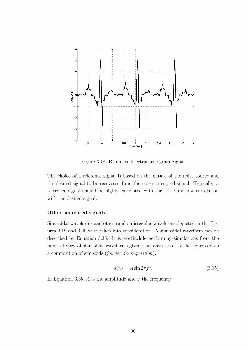
Figure 3.18: Reference Electrocardiogram Signal
The choice of a reference signal is based on the nature of the noise source and
the desired signal to be recovered from the noise corrupted signal. Typically, a
reference signal should be highly correlated with the noise and low correlation
with the desired signal.
Other simulated signals
Sinusoidal waveforms and other random irregular waveforms depicted in the Fig-
ures 3.19 and 3.20 were taken into consideration. A sinusoidal waveform can be
described by Equation 3.35. It is worthwhile performing simulations from the
point of view of sinusoidal waveforms given that any signal can be expressed as
a composition of sinusoids (fourier decomposition).
s(n) = A sin 2πfn (3.35)
In Equation 3.35, A is the amplitude and f the frequency.
36
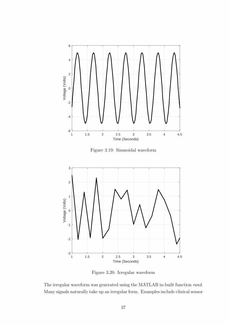
1 1.5 2 2.5 3 3.5 4 4.5
Time (Seconds)
-6
-4
-2
0
2
4
6
Vol
tage
(V
olts
)
Figure 3.19: Sinusoidal waveform
1 1.5 2 2.5 3 3.5 4 4.5
Time (Seconds)
-3
-2
-1
0
1
2
3
Vol
tage
(V
olts
)
Figure 3.20: Irregular waveform
The irregular waveform was generated using the MATLAB in-built function rand.
Many signals naturally take up an irregular form. Examples include clinical sensor
37
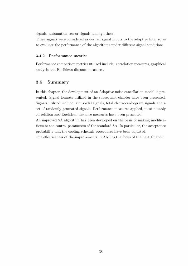
signals, automation sensor signals among others.
These signals were considered as desired signal inputs to the adaptive filter so as
to evaluate the performance of the algorithms under different signal conditions.
3.4.2 Performance metrics
Performance comparison metrics utilized include: correlation measures, graphical
analysis and Euclidean distance measures.
3.5 Summary
In this chapter, the development of an Adaptive noise cancellation model is pre-
sented. Signal formats utilized in the subsequent chapter have been presented.
Signals utilized include: sinusoidal signals, fetal electrocardiogram signals and a
set of randomly generated signals. Performance measures applied, most notably
correlation and Euclidean distance measures have been presented.
An improved SA algorithm has been developed on the basis of making modifica-
tions to the control parameters of the standard SA. In particular, the acceptance
probability and the cooling schedule procedures have been adjusted.
The effectiveness of the improvements in ANC is the focus of the next Chapter.
38

CHAPTER FOUR
RESULTS AND DISCUSSION
Comparisons are hereby done between the performance of SA, its improved ver-
sion, LMS and NLMS algorithms under a variety of signal and noise conditions
in ANC. The LMS and NLMS algorithm schemes utilized follow those utilized
in (Hameed, 2012). Performance measures taken into consideration are conver-
gence speed and final solution accuracy (error amount) measured as a correlation
value. All algorithms are run for equal adaptation durations. Consequently, a
better convergence rate can be deduced from higher waveform correlation values
between desired waveform and adaptation result waveform.
4.1 Comparison of the improved SA algorithm against the
standard SA algorithm in adaptive noise cancellation
In this Section, the effectiveness of the SA algorithm improvements proposed in
Section 3.2 are analyzed in a speech signal noise cancellation application. The
utilized speech signal is as described in Section 3.3.2.
Figures 4.21 and 4.23 are representative of the results obtained upon application
of the improved and standard SA algorithms in adaptive noise cancellation. The
figures portray the outcomes associated with two audio channels (stereo audio
scenario).
39
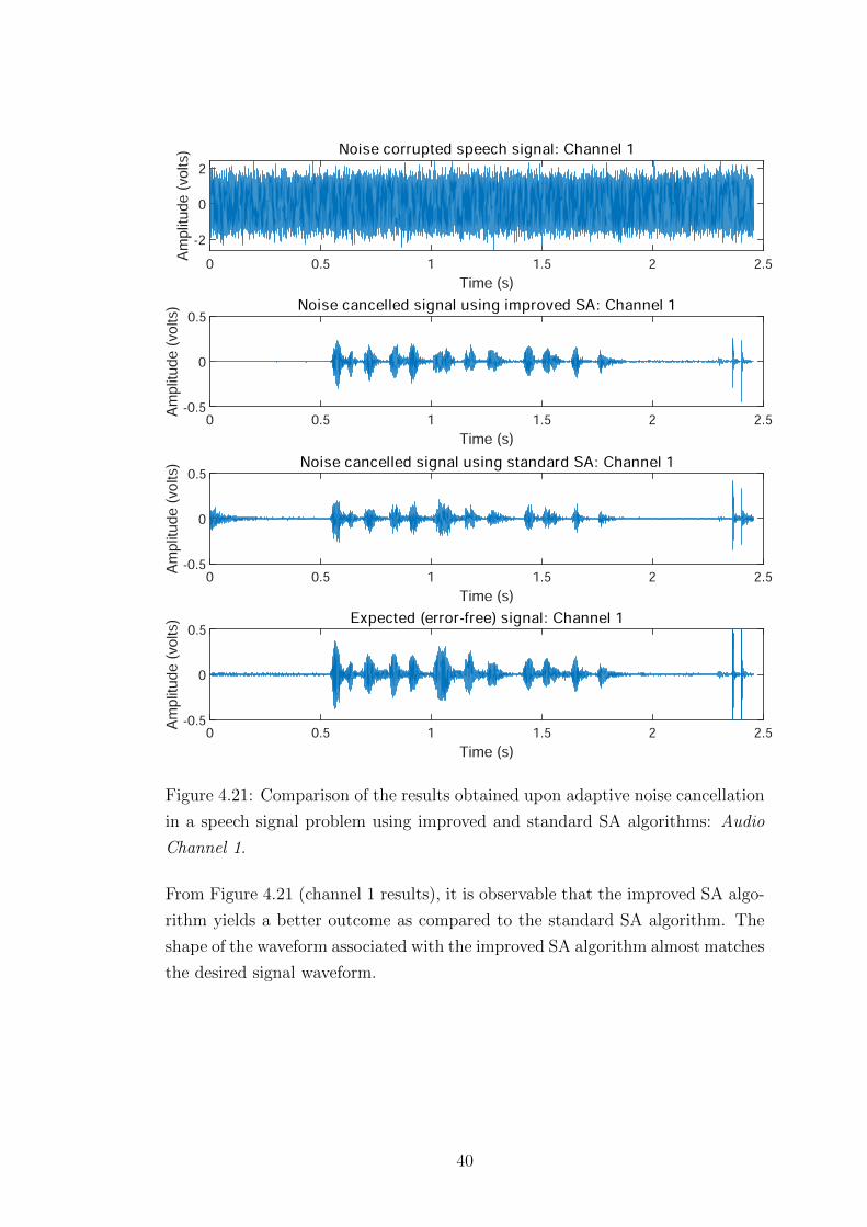
ð ðòë ï ïòë î îòë
Ì·³» ø÷ ïðë
óî
ð
î
Ò±·» ½±®®«°¬»¼ °»»½¸ ·¹²¿´æ ݸ¿²²»´ ï
ð ðòë ï ïòë î îòë
Ì·³» ø÷ ïðë
óðòë
ð
ðòëÒ±·» ½¿²½»´´»¼ ·¹²¿´ «·²¹ ·³°®±ª»¼ Íßæ ݸ¿²²»´ ï
ð ðòë ï ïòë î îòë
Ì·³» ø÷ ïðë
óðòë
ð
ðòëÒ±·» ½¿²½»´´»¼ ·¹²¿´ «·²¹ ¬¿²¼¿®¼ Íßæ ݸ¿²²»´ ï
ð ðòë ï ïòë î îòë
Ì·³» ø÷ ïðë
óðòë
ð
ðòëÛ¨°»½¬»¼ ø»®®±®óº®»»÷ ·¹²¿´æ ݸ¿²²»´ ï
Figure 4.21: Comparison of the results obtained upon adaptive noise cancellation
in a speech signal problem using improved and standard SA algorithms: Audio
Channel 1.
From Figure 4.21 (channel 1 results), it is observable that the improved SA algo-
rithm yields a better outcome as compared to the standard SA algorithm. The
shape of the waveform associated with the improved SA algorithm almost matches
the desired signal waveform.
40
ð ðòë ï ïòë î îòë
Ì·³» ø÷ ïðë
óî
ð
î
Ò±·» ½±®®«°¬»¼ °»»½¸ ·¹²¿´æ ݸ¿²²»´ î
ð ðòë ï ïòë î îòë
Ì·³» ø÷ ïðë
óðòë
ð
ðòëÒ±·» ½¿²½»´´»¼ ·¹²¿´ «·²¹ ·³°®±ª»¼ Íßæ ݸ¿²²»´ î
ð ðòë ï ïòë î îòë
Ì·³» ø÷ ïðë
óðòë
ð
ðòëÒ±·» ½¿²½»´´»¼ ·¹²¿´ «·²¹ ¬¿²¼¿®¼ Íßæ ݸ¿²²»´ î
ð ðòë ï ïòë î îòë
Ì·³» ø÷ ïðë
óðòë
ð
ðòëÛ¨°»½¬»¼ ø»®®±®óº®»»÷ ·¹²¿´æ ݸ¿²²»´ î
Figure 4.22: Comparison of the results obtained upon adaptive noise cancellation
in a speech signal problem using improved and standard SA algorithms: Audio
Channel 2.
From Figure 4.23 (channel 2 results), it is observable that the improved SA algo-
rithm yields a better outcome as compared to the standard SA algorithm. The
shape of the waveform associated with the improved SA algorithm almost matches
the desired signal waveform.
Comparative correlation values are given in Table 4.4. The improved and stan-
dard SA algorithm correlation results values have been obtained upon averaging
the outcome of 50 independent adaptive noise cancellation runs.
41

Table 4.4: Comparative correlation values.
Channel 1 Channel 2
Correlation between the desired signal and: Mean SD Mean SD
Corrupted signal 0.0796 N/A 0.0805 N/A
ISA algorithm noise cancellation result 0.7418 0.013 0.7523 0.012
SA algorithm noise cancellation result 0.5609 0.014 0.5349 0.017
0
0.1
0.2
0.3
0.4
0.5
0.6
0.7
0.8
Channel 1 Channel 2
Correlation values
ISA SA
Figure 4.23: A graph portraying the correlation values presented in Table 4.4.
The results presented herein portray the efficacy of the SA algorithm improve-
ments presented in Section 3.2.
4.2 Comparison of the improved simulated annealing al-
gorithm in adaptive noise cancellation with standard
SA, NLMS and LMS algorithms
In this section the use of improved and standard SA algorithms in ANC is ana-
lyzed against the commonly used NLMS and LMS algorithms. Adaptive weight
generation is studied comprehensively under a variety of sinusoidal signal and
noise conditions. Varying signal frequencies have been utilized to give a com-
prehensive algorithm performance comparison. High frequency sinusoidal signals
featuring AWGN have been used as the noise signals. The improved SA algo-
42
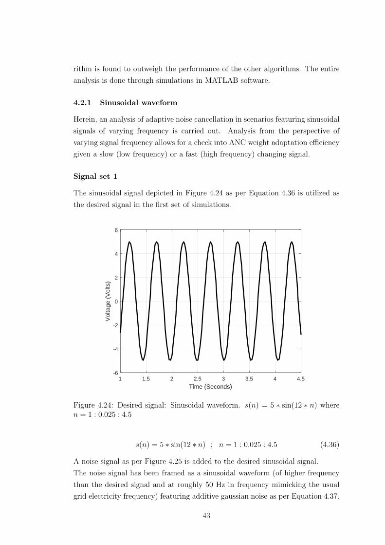
rithm is found to outweigh the performance of the other algorithms. The entire
analysis is done through simulations in MATLAB software.
4.2.1 Sinusoidal waveform
Herein, an analysis of adaptive noise cancellation in scenarios featuring sinusoidal
signals of varying frequency is carried out. Analysis from the perspective of
varying signal frequency allows for a check into ANC weight adaptation efficiency
given a slow (low frequency) or a fast (high frequency) changing signal.
Signal set 1
The sinusoidal signal depicted in Figure 4.24 as per Equation 4.36 is utilized as
the desired signal in the first set of simulations.
1 1.5 2 2.5 3 3.5 4 4.5
Time (Seconds)
-6
-4
-2
0
2
4
6
Vol
tage
(V
olts
)
Figure 4.24: Desired signal: Sinusoidal waveform. s(n) = 5 ∗ sin(12 ∗ n) wheren = 1 : 0.025 : 4.5
s(n) = 5 ∗ sin(12 ∗ n) ; n = 1 : 0.025 : 4.5 (4.36)
A noise signal as per Figure 4.25 is added to the desired sinusoidal signal.
The noise signal has been framed as a sinusoidal waveform (of higher frequency
than the desired signal and at roughly 50 Hz in frequency mimicking the usual
grid electricity frequency) featuring additive gaussian noise as per Equation 4.37.
43
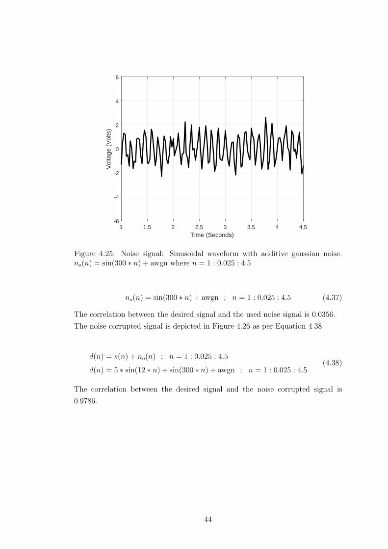
1 1.5 2 2.5 3 3.5 4 4.5
Time (Seconds)
-6
-4
-2
0
2
4
6
Vol
tage
(V
olts
)
Figure 4.25: Noise signal: Sinusoidal waveform with additive gaussian noise.no(n) = sin(300 ∗ n) + awgn where n = 1 : 0.025 : 4.5
no(n) = sin(300 ∗ n) + awgn ; n = 1 : 0.025 : 4.5 (4.37)
The correlation between the desired signal and the used noise signal is 0.0356.
The noise corrupted signal is depicted in Figure 4.26 as per Equation 4.38.
d(n) = s(n) + no(n) ; n = 1 : 0.025 : 4.5
d(n) = 5 ∗ sin(12 ∗ n) + sin(300 ∗ n) + awgn ; n = 1 : 0.025 : 4.5(4.38)
The correlation between the desired signal and the noise corrupted signal is
0.9786.
44
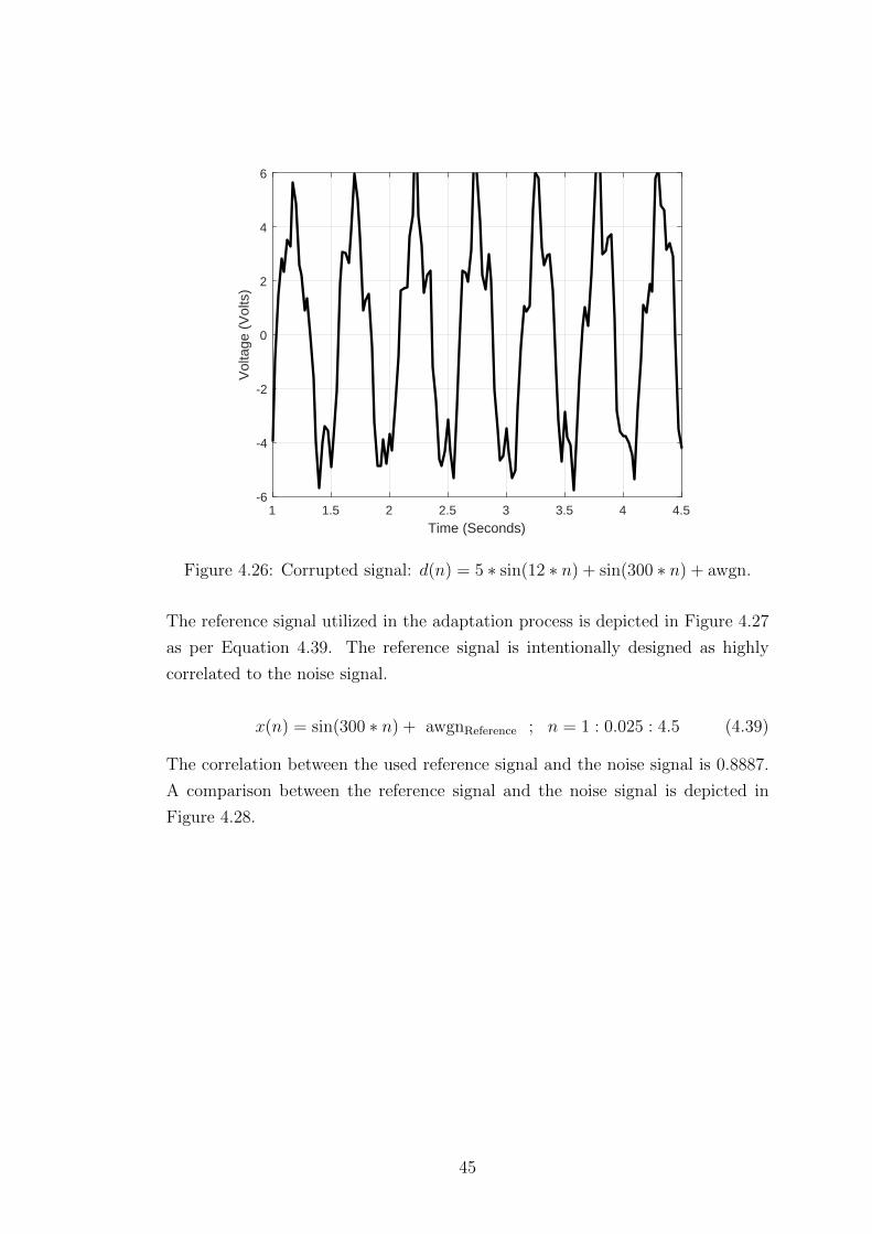
1 1.5 2 2.5 3 3.5 4 4.5
Time (Seconds)
-6
-4
-2
0
2
4
6
Vol
tage
(V
olts
)
Figure 4.26: Corrupted signal: d(n) = 5 ∗ sin(12 ∗ n) + sin(300 ∗ n) + awgn.
The reference signal utilized in the adaptation process is depicted in Figure 4.27
as per Equation 4.39. The reference signal is intentionally designed as highly
correlated to the noise signal.
x(n) = sin(300 ∗ n) + awgnReference ; n = 1 : 0.025 : 4.5 (4.39)
The correlation between the used reference signal and the noise signal is 0.8887.
A comparison between the reference signal and the noise signal is depicted in
Figure 4.28.
45
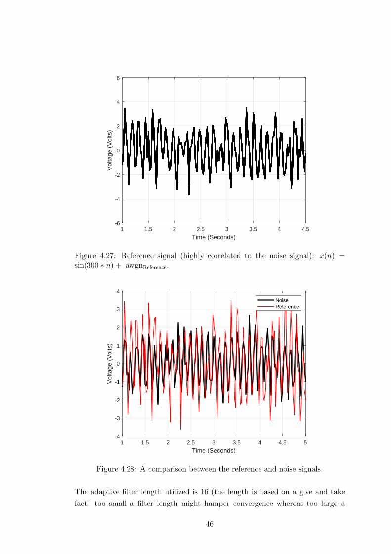
1 1.5 2 2.5 3 3.5 4 4.5
Time (Seconds)
-6
-4
-2
0
2
4
6
Vol
tage
(V
olts
)
Figure 4.27: Reference signal (highly correlated to the noise signal): x(n) =sin(300 ∗ n) + awgnReference.
1 1.5 2 2.5 3 3.5 4 4.5 5
Time (Seconds)
-4
-3
-2
-1
0
1
2
3
4
Vol
tage
(V
olts
)
NoiseReference
Figure 4.28: A comparison between the reference and noise signals.
The adaptive filter length utilized is 16 (the length is based on a give and take
fact: too small a filter length might hamper convergence whereas too large a
46
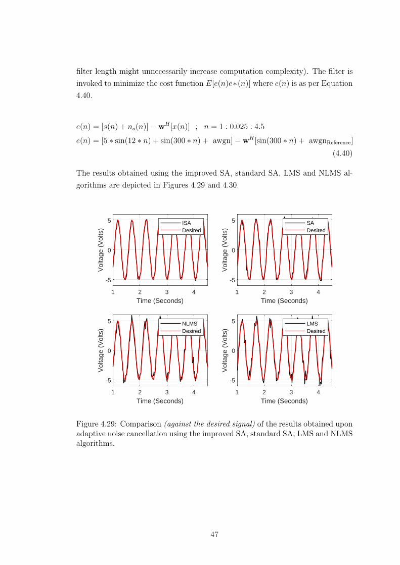
filter length might unnecessarily increase computation complexity). The filter is
invoked to minimize the cost function E[e(n)e∗(n)] where e(n) is as per Equation
4.40.
e(n) = [s(n) + no(n)]−wH [x(n)] ; n = 1 : 0.025 : 4.5
e(n) = [5 ∗ sin(12 ∗ n) + sin(300 ∗ n) + awgn]−wH [sin(300 ∗ n) + awgnReference]
(4.40)
The results obtained using the improved SA, standard SA, LMS and NLMS al-
gorithms are depicted in Figures 4.29 and 4.30.
1 2 3 4
Time (Seconds)
-5
0
5
Vol
tage
(V
olts
)
ISADesired
1 2 3 4
Time (Seconds)
-5
0
5V
olta
ge (
Vol
ts)
SADesired
1 2 3 4
Time (Seconds)
-5
0
5
Vol
tage
(V
olts
)
NLMSDesired
1 2 3 4
Time (Seconds)
-5
0
5
Vol
tage
(V
olts
)
LMSDesired
Figure 4.29: Comparison (against the desired signal) of the results obtained uponadaptive noise cancellation using the improved SA, standard SA, LMS and NLMSalgorithms.
47
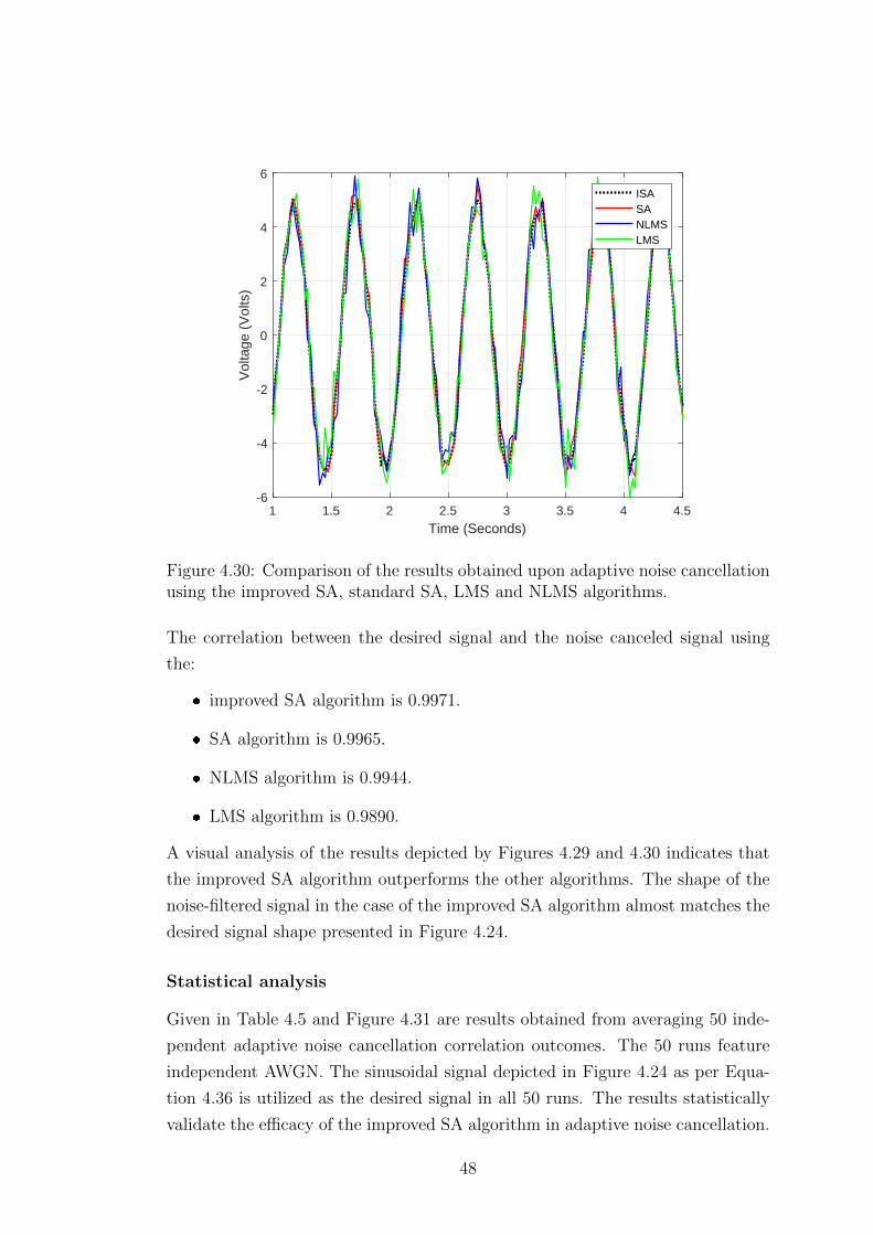
1 1.5 2 2.5 3 3.5 4 4.5
Time (Seconds)
-6
-4
-2
0
2
4
6
Vol
tage
(V
olts
)
ISASANLMSLMS
Figure 4.30: Comparison of the results obtained upon adaptive noise cancellationusing the improved SA, standard SA, LMS and NLMS algorithms.
The correlation between the desired signal and the noise canceled signal using
the:
� improved SA algorithm is 0.9971.
� SA algorithm is 0.9965.
� NLMS algorithm is 0.9944.
� LMS algorithm is 0.9890.
A visual analysis of the results depicted by Figures 4.29 and 4.30 indicates that
the improved SA algorithm outperforms the other algorithms. The shape of the
noise-filtered signal in the case of the improved SA algorithm almost matches the
desired signal shape presented in Figure 4.24.
Statistical analysis
Given in Table 4.5 and Figure 4.31 are results obtained from averaging 50 inde-
pendent adaptive noise cancellation correlation outcomes. The 50 runs feature
independent AWGN. The sinusoidal signal depicted in Figure 4.24 as per Equa-
tion 4.36 is utilized as the desired signal in all 50 runs. The results statistically
validate the efficacy of the improved SA algorithm in adaptive noise cancellation.
48

Table 4.5: Comparative correlation values.
Correlation between the desired signal and: Mean SD
Corrupted signal 0.8889 0.0001
ISA algorithm noise cancellation result 0.9984 0.0001
SA algorithm noise cancellation result 0.9967 0.0013
NLMS algorithm noise cancellation result 0.9943 0.0019
LMS algorithm noise cancellation result 0.9887 0.0023
0.82
0.84
0.86
0.88
0.9
0.92
0.94
0.96
0.98
1
1.02
Corrupted
signal
ISA SA NLMS LMS
Average correlation values
Figure 4.31: A graph portraying the correlation values presented in Table 4.5.
Reference signal selection
It is usually desired that the selected reference signal be highly correlated to
the noise in question in an adaptive signal processing scheme. This requirement
is confirmed in the set of results presented herein. In a particular simulation,
the correlation between the used reference signal and the noise corrupted signal
is 0.5981. A comparison between the reference signal and the noise signal is
depicted in Figure 4.32.
49
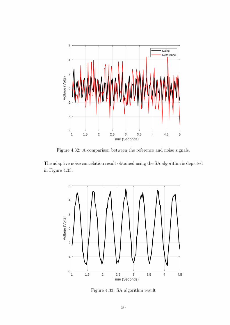
1 1.5 2 2.5 3 3.5 4 4.5 5
Time (Seconds)
-6
-4
-2
0
2
4
6
Vol
tage
(V
olts
)
NoiseReference
Figure 4.32: A comparison between the reference and noise signals.
The adaptive noise cancelation result obtained using the SA algorithm is depicted
in Figure 4.33.
1 1.5 2 2.5 3 3.5 4 4.5
Time (Seconds)
-6
-4
-2
0
2
4
6
Vol
tage
(V
olts
)
Figure 4.33: SA algorithm result
50
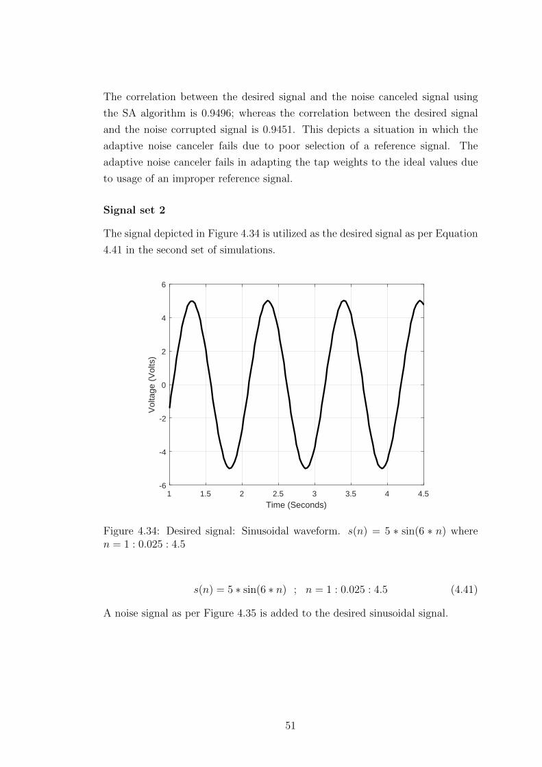
The correlation between the desired signal and the noise canceled signal using
the SA algorithm is 0.9496; whereas the correlation between the desired signal
and the noise corrupted signal is 0.9451. This depicts a situation in which the
adaptive noise canceler fails due to poor selection of a reference signal. The
adaptive noise canceler fails in adapting the tap weights to the ideal values due
to usage of an improper reference signal.
Signal set 2
The signal depicted in Figure 4.34 is utilized as the desired signal as per Equation
4.41 in the second set of simulations.
1 1.5 2 2.5 3 3.5 4 4.5
Time (Seconds)
-6
-4
-2
0
2
4
6
Vol
tage
(V
olts
)
Figure 4.34: Desired signal: Sinusoidal waveform. s(n) = 5 ∗ sin(6 ∗ n) wheren = 1 : 0.025 : 4.5
s(n) = 5 ∗ sin(6 ∗ n) ; n = 1 : 0.025 : 4.5 (4.41)
A noise signal as per Figure 4.35 is added to the desired sinusoidal signal.
51
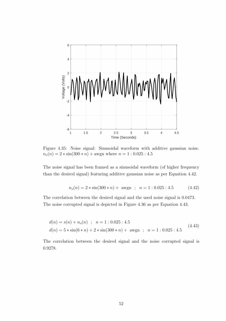
1 1.5 2 2.5 3 3.5 4 4.5
Time (Seconds)
-6
-4
-2
0
2
4
6
Vol
tage
(V
olts
)
Figure 4.35: Noise signal: Sinusoidal waveform with additive gaussian noise.no(n) = 2 ∗ sin(300 ∗ n) + awgn where n = 1 : 0.025 : 4.5
The noise signal has been framed as a sinusoidal waveform (of higher frequency
than the desired signal) featuring additive gaussian noise as per Equation 4.42.
no(n) = 2 ∗ sin(300 ∗ n) + awgn ; n = 1 : 0.025 : 4.5 (4.42)
The correlation between the desired signal and the used noise signal is 0.0473.
The noise corrupted signal is depicted in Figure 4.36 as per Equation 4.43.
d(n) = s(n) + no(n) ; n = 1 : 0.025 : 4.5
d(n) = 5 ∗ sin(6 ∗ n) + 2 ∗ sin(300 ∗ n) + awgn ; n = 1 : 0.025 : 4.5(4.43)
The correlation between the desired signal and the noise corrupted signal is
0.9278.
52
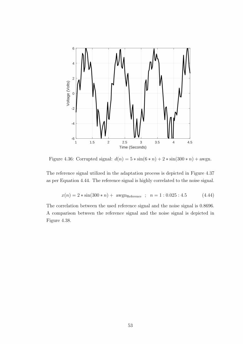
1 1.5 2 2.5 3 3.5 4 4.5
Time (Seconds)
-6
-4
-2
0
2
4
6
Vol
tage
(V
olts
)
Figure 4.36: Corrupted signal: d(n) = 5 ∗ sin(6 ∗ n) + 2 ∗ sin(300 ∗ n) + awgn.
The reference signal utilized in the adaptation process is depicted in Figure 4.37
as per Equation 4.44. The reference signal is highly correlated to the noise signal.
x(n) = 2 ∗ sin(300 ∗ n) + awgnReference ; n = 1 : 0.025 : 4.5 (4.44)
The correlation between the used reference signal and the noise signal is 0.8696.
A comparison between the reference signal and the noise signal is depicted in
Figure 4.38.
53
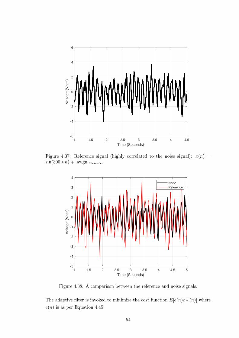
1 1.5 2 2.5 3 3.5 4 4.5
Time (Seconds)
-6
-4
-2
0
2
4
6
Vol
tage
(V
olts
)
Figure 4.37: Reference signal (highly correlated to the noise signal): x(n) =sin(300 ∗ n) + awgnReference.
1 1.5 2 2.5 3 3.5 4 4.5 5
Time (Seconds)
-5
-4
-3
-2
-1
0
1
2
3
4
Vol
tage
(V
olts
)
NoiseReference
Figure 4.38: A comparison between the reference and noise signals.
The adaptive filter is invoked to minimize the cost function E[e(n)e ∗ (n)] where
e(n) is as per Equation 4.45.
54
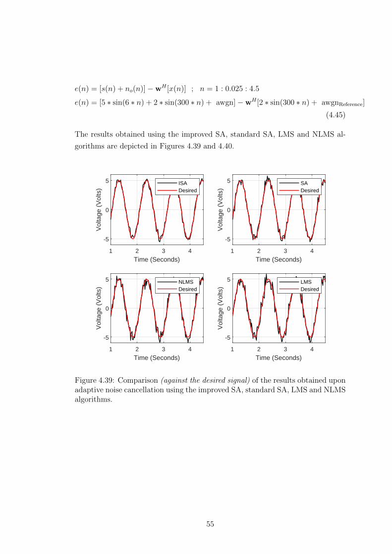
e(n) = [s(n) + no(n)]−wH [x(n)] ; n = 1 : 0.025 : 4.5
e(n) = [5 ∗ sin(6 ∗ n) + 2 ∗ sin(300 ∗ n) + awgn]−wH [2 ∗ sin(300 ∗ n) + awgnReference]
(4.45)
The results obtained using the improved SA, standard SA, LMS and NLMS al-
gorithms are depicted in Figures 4.39 and 4.40.
1 2 3 4
Time (Seconds)
-5
0
5
Vol
tage
(V
olts
)
ISADesired
1 2 3 4
Time (Seconds)
-5
0
5
Vol
tage
(V
olts
)
SADesired
1 2 3 4
Time (Seconds)
-5
0
5
Vol
tage
(V
olts
)
NLMSDesired
1 2 3 4
Time (Seconds)
-5
0
5
Vol
tage
(V
olts
)
LMSDesired
Figure 4.39: Comparison (against the desired signal) of the results obtained uponadaptive noise cancellation using the improved SA, standard SA, LMS and NLMSalgorithms.
55
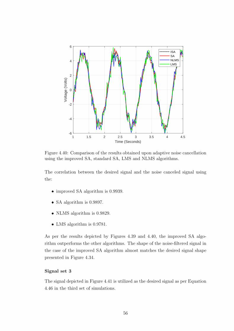
1 1.5 2 2.5 3 3.5 4 4.5
Time (Seconds)
-6
-4
-2
0
2
4
6
Vol
tage
(V
olts
)
ISASANLMSLMS
Figure 4.40: Comparison of the results obtained upon adaptive noise cancellationusing the improved SA, standard SA, LMS and NLMS algorithms.
The correlation between the desired signal and the noise canceled signal using
the:
� improved SA algorithm is 0.9939.
� SA algorithm is 0.9897.
� NLMS algorithm is 0.9829.
� LMS algorithm is 0.9781.
As per the results depicted by Figures 4.39 and 4.40, the improved SA algo-
rithm outperforms the other algorithms. The shape of the noise-filtered signal in
the case of the improved SA algorithm almost matches the desired signal shape
presented in Figure 4.34.
Signal set 3
The signal depicted in Figure 4.41 is utilized as the desired signal as per Equation
4.46 in the third set of simulations.
56
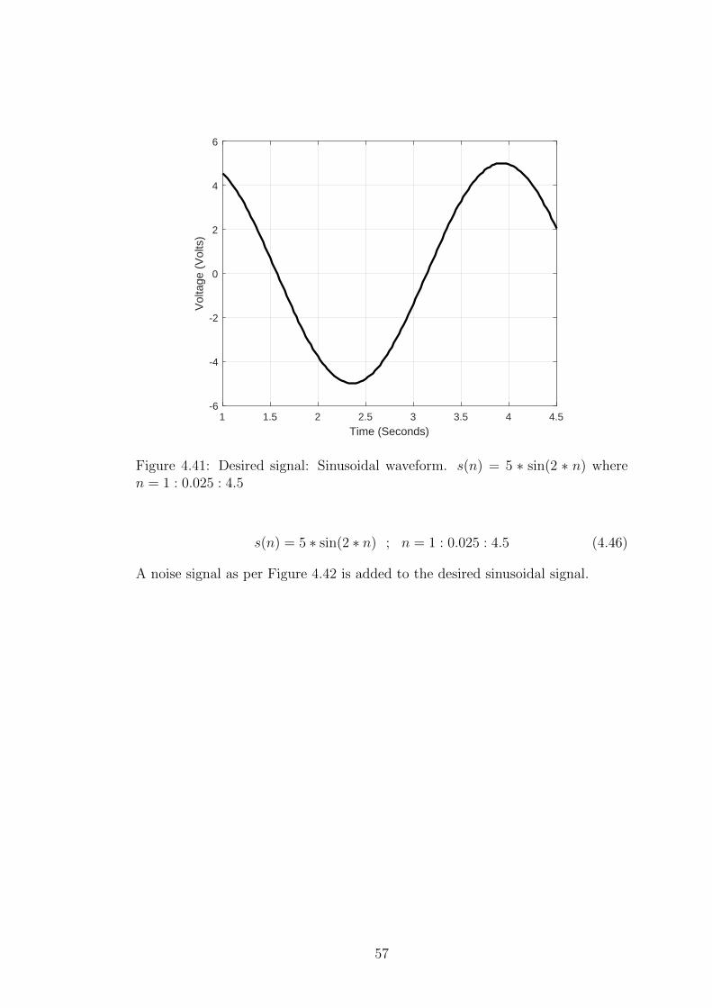
1 1.5 2 2.5 3 3.5 4 4.5
Time (Seconds)
-6
-4
-2
0
2
4
6
Vol
tage
(V
olts
)
Figure 4.41: Desired signal: Sinusoidal waveform. s(n) = 5 ∗ sin(2 ∗ n) wheren = 1 : 0.025 : 4.5
s(n) = 5 ∗ sin(2 ∗ n) ; n = 1 : 0.025 : 4.5 (4.46)
A noise signal as per Figure 4.42 is added to the desired sinusoidal signal.
57
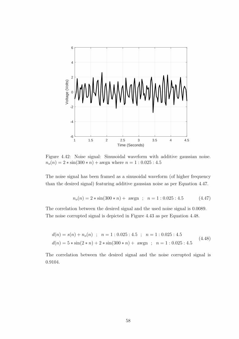
1 1.5 2 2.5 3 3.5 4 4.5
Time (Seconds)
-6
-4
-2
0
2
4
6
Vol
tage
(V
olts
)
Figure 4.42: Noise signal: Sinusoidal waveform with additive gaussian noise.no(n) = 2 ∗ sin(300 ∗ n) + awgn where n = 1 : 0.025 : 4.5
The noise signal has been framed as a sinusoidal waveform (of higher frequency
than the desired signal) featuring additive gaussian noise as per Equation 4.47.
no(n) = 2 ∗ sin(300 ∗ n) + awgn ; n = 1 : 0.025 : 4.5 (4.47)
The correlation between the desired signal and the used noise signal is 0.0089.
The noise corrupted signal is depicted in Figure 4.43 as per Equation 4.48.
d(n) = s(n) + no(n) ; n = 1 : 0.025 : 4.5 ; n = 1 : 0.025 : 4.5
d(n) = 5 ∗ sin(2 ∗ n) + 2 ∗ sin(300 ∗ n) + awgn ; n = 1 : 0.025 : 4.5(4.48)
The correlation between the desired signal and the noise corrupted signal is
0.9104.
58
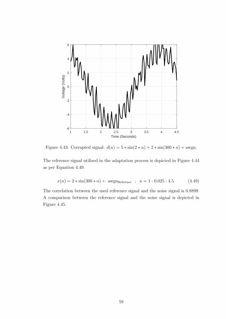
1 1.5 2 2.5 3 3.5 4 4.5
Time (Seconds)
-6
-4
-2
0
2
4
6
Vol
tage
(V
olts
)
Figure 4.43: Corrupted signal: d(n) = 5 ∗ sin(2 ∗ n) + 2 ∗ sin(300 ∗ n) + awgn.
The reference signal utilized in the adaptation process is depicted in Figure 4.44
as per Equation 4.49.
x(n) = 2 ∗ sin(300 ∗ n) + awgnReference ; n = 1 : 0.025 : 4.5 (4.49)
The correlation between the used reference signal and the noise signal is 0.8899.
A comparison between the reference signal and the noise signal is depicted in
Figure 4.45.
59
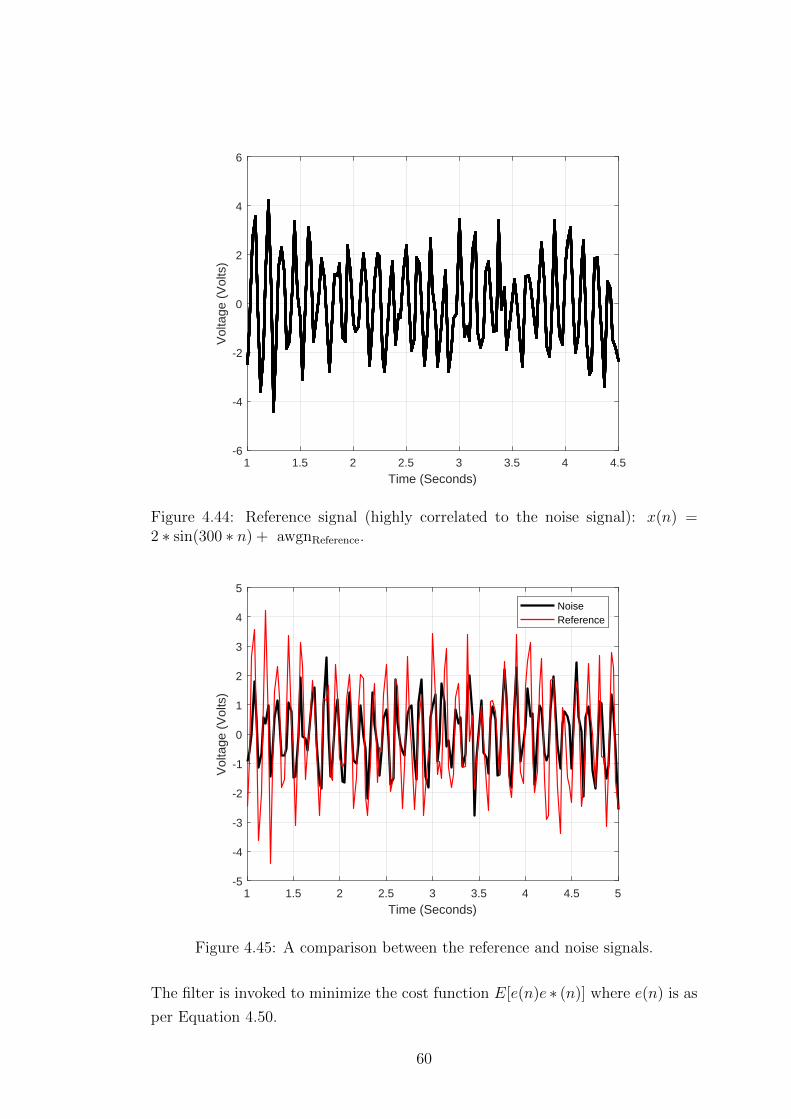
1 1.5 2 2.5 3 3.5 4 4.5
Time (Seconds)
-6
-4
-2
0
2
4
6
Vol
tage
(V
olts
)
Figure 4.44: Reference signal (highly correlated to the noise signal): x(n) =2 ∗ sin(300 ∗ n) + awgnReference.
1 1.5 2 2.5 3 3.5 4 4.5 5
Time (Seconds)
-5
-4
-3
-2
-1
0
1
2
3
4
5
Vol
tage
(V
olts
)
NoiseReference
Figure 4.45: A comparison between the reference and noise signals.
The filter is invoked to minimize the cost function E[e(n)e ∗ (n)] where e(n) is as
per Equation 4.50.
60
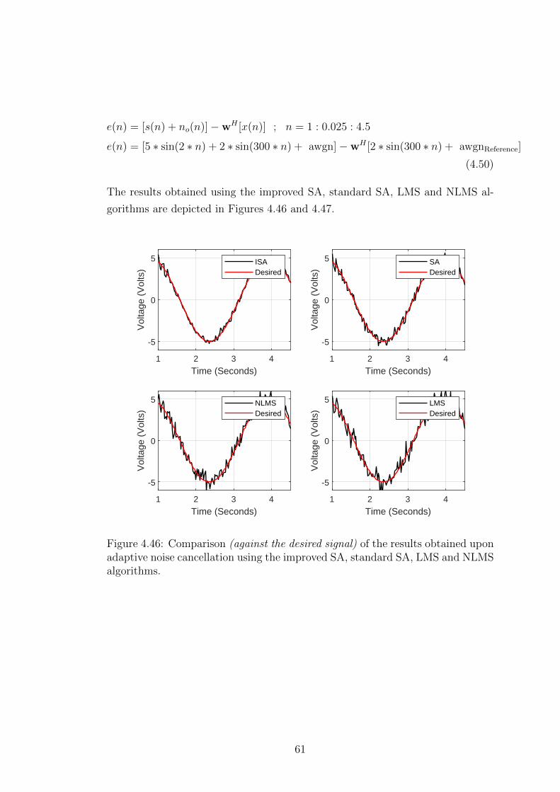
e(n) = [s(n) + no(n)]−wH [x(n)] ; n = 1 : 0.025 : 4.5
e(n) = [5 ∗ sin(2 ∗ n) + 2 ∗ sin(300 ∗ n) + awgn]−wH [2 ∗ sin(300 ∗ n) + awgnReference]
(4.50)
The results obtained using the improved SA, standard SA, LMS and NLMS al-
gorithms are depicted in Figures 4.46 and 4.47.
1 2 3 4
Time (Seconds)
-5
0
5
Vol
tage
(V
olts
)
ISADesired
1 2 3 4
Time (Seconds)
-5
0
5
Vol
tage
(V
olts
)
SADesired
1 2 3 4
Time (Seconds)
-5
0
5
Vol
tage
(V
olts
)
NLMSDesired
1 2 3 4
Time (Seconds)
-5
0
5
Vol
tage
(V
olts
)
LMSDesired
Figure 4.46: Comparison (against the desired signal) of the results obtained uponadaptive noise cancellation using the improved SA, standard SA, LMS and NLMSalgorithms.
61

1 1.5 2 2.5 3 3.5 4 4.5
Time (Seconds)
-6
-4
-2
0
2
4
6
Vol
tage
(V
olts
)
ISASANLMSLMS
Figure 4.47: Comparison of the results obtained upon adaptive noise cancellationusing the improved SA, standard SA, LMS and NLMS algorithms.
The correlation between the desired signal and the noise canceled signal using
the:
� improved SA algorithm is 0.9883.
� SA algorithm is 0.9851.
� NLMS algorithm is 0.9833.
� LMS algorithm is 0.9786.
As per the results depicted by Figures 4.46 and 4.47, the improved SA algo-
rithm outperforms the other algorithms. The shape of the noise-filtered signal in
the case of the improved SA algorithm almost matches the desired signal shape
presented in Figure 4.41.
Discussion
The improved SA algorithm is found to generate better results than the other
algorithms in all simulated scenarios. The algorithms were run for equal dura-
tions (4.5 seconds). Lower noise levels over a uniform noise cancellation period
62

are achieved using the improved SA algorithm as compared to the other algo-
rithms as per Figures 4.29, 4.30, 4.39, 4.40, 4.46 and 4.47. This indicates better
convergence speed when using the improved SA algorithm as compared to the
other algorithms.
Generated signal graphs and correlation values relay the following information:
� The improved SA algorithm yields a less noise corrupted signal.
� Irrespective of the waveform frequency involved, the improved SA algorithm
produces better results.
The improved SA algorithm yields a noise-cancelled signal output more correlated
with the desired signal as compared to the other algorithms.
Deductions
Adaptive noise cancellers play a crucial role in modern communication networks.
The role of efficient adaptation algorithms for use in adaptive noise cancellers
cannot be underestimated. Generally the improved and standard SA algorithms
are found to be more efficient than the NLMS and LMS algorithms in MMSE
based adaptive noise cancellation as far as sinusoidal signals are concerned.
4.2.2 Irregular waveform
In this section the use of improved and standard SA algorithms in ANC is an-
alyzed against the commonly used NLMS and LMS algorithms in an irregularly
shaped signal case. An irregularly shaped signal accommodates a wide variety of
signals that feature in many practical occurrences. A randomly generated noise
signal has been used. The improved SA algorithm is found to outweigh the per-
formance of the other algorithms. The entire analysis is done through simulations
in MATLAB software.
The signal depicted in Figure 4.48 is utilized as the desired signal as per Equation
4.51 in the second set of simulations.
s(n) = rand(n; [−2.5 : 2.5]) ; n = 1 : 0.2 : 4.5 (4.51)
63
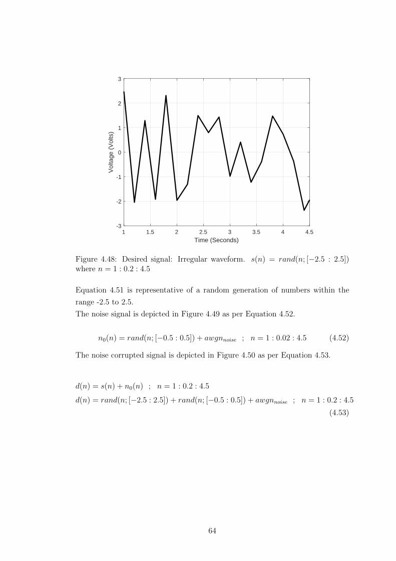
1 1.5 2 2.5 3 3.5 4 4.5
Time (Seconds)
-3
-2
-1
0
1
2
3
Vol
tage
(V
olts
)
Figure 4.48: Desired signal: Irregular waveform. s(n) = rand(n; [−2.5 : 2.5])where n = 1 : 0.2 : 4.5
Equation 4.51 is representative of a random generation of numbers within the
range -2.5 to 2.5.
The noise signal is depicted in Figure 4.49 as per Equation 4.52.
n0(n) = rand(n; [−0.5 : 0.5]) + awgnnoise ; n = 1 : 0.02 : 4.5 (4.52)
The noise corrupted signal is depicted in Figure 4.50 as per Equation 4.53.
d(n) = s(n) + n0(n) ; n = 1 : 0.2 : 4.5
d(n) = rand(n; [−2.5 : 2.5]) + rand(n; [−0.5 : 0.5]) + awgnnoise ; n = 1 : 0.2 : 4.5
(4.53)
64
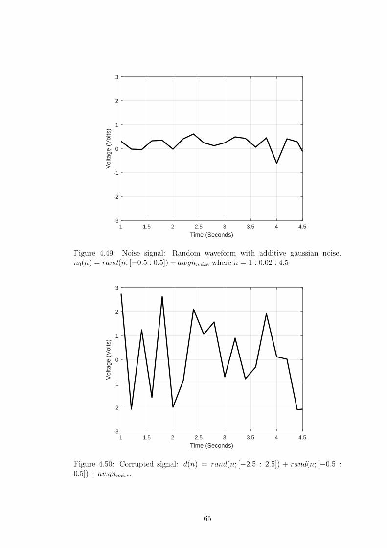
1 1.5 2 2.5 3 3.5 4 4.5
Time (Seconds)
-3
-2
-1
0
1
2
3
Vol
tage
(V
olts
)
Figure 4.49: Noise signal: Random waveform with additive gaussian noise.n0(n) = rand(n; [−0.5 : 0.5]) + awgnnoise where n = 1 : 0.02 : 4.5
1 1.5 2 2.5 3 3.5 4 4.5
Time (Seconds)
-3
-2
-1
0
1
2
3
Vol
tage
(V
olts
)
Figure 4.50: Corrupted signal: d(n) = rand(n; [−2.5 : 2.5]) + rand(n; [−0.5 :0.5]) + awgnnoise.
65

The reference utilized signal is depicted in Figure 4.51 as per Equation 4.54.
1 1.5 2 2.5 3 3.5 4 4.5
Time (Seconds)
-3
-2
-1
0
1
2
3
Vol
tage
(V
olts
)
Figure 4.51: Reference signal (highly correlated to the noise signal): x(n) =n0(n) + awgnref .
x(n) = n0(n) + awgnref ; n = 1 : 0.2 : 4.5 (4.54)
A comparison of the noise and the reference signals is depicted in Figure 4.52.
The results obtained using the improved SA, standard SA, LMS and NLMS al-
gorithms are depicted in Figures 4.53 and 4.54.
66
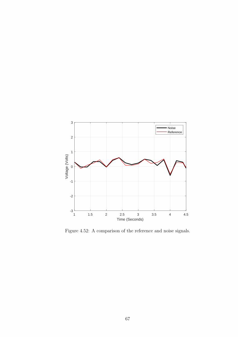
1 1.5 2 2.5 3 3.5 4 4.5
Time (Seconds)
-3
-2
-1
0
1
2
3
Vol
tage
(V
olts
)
NoiseReference
Figure 4.52: A comparison of the reference and noise signals.
67
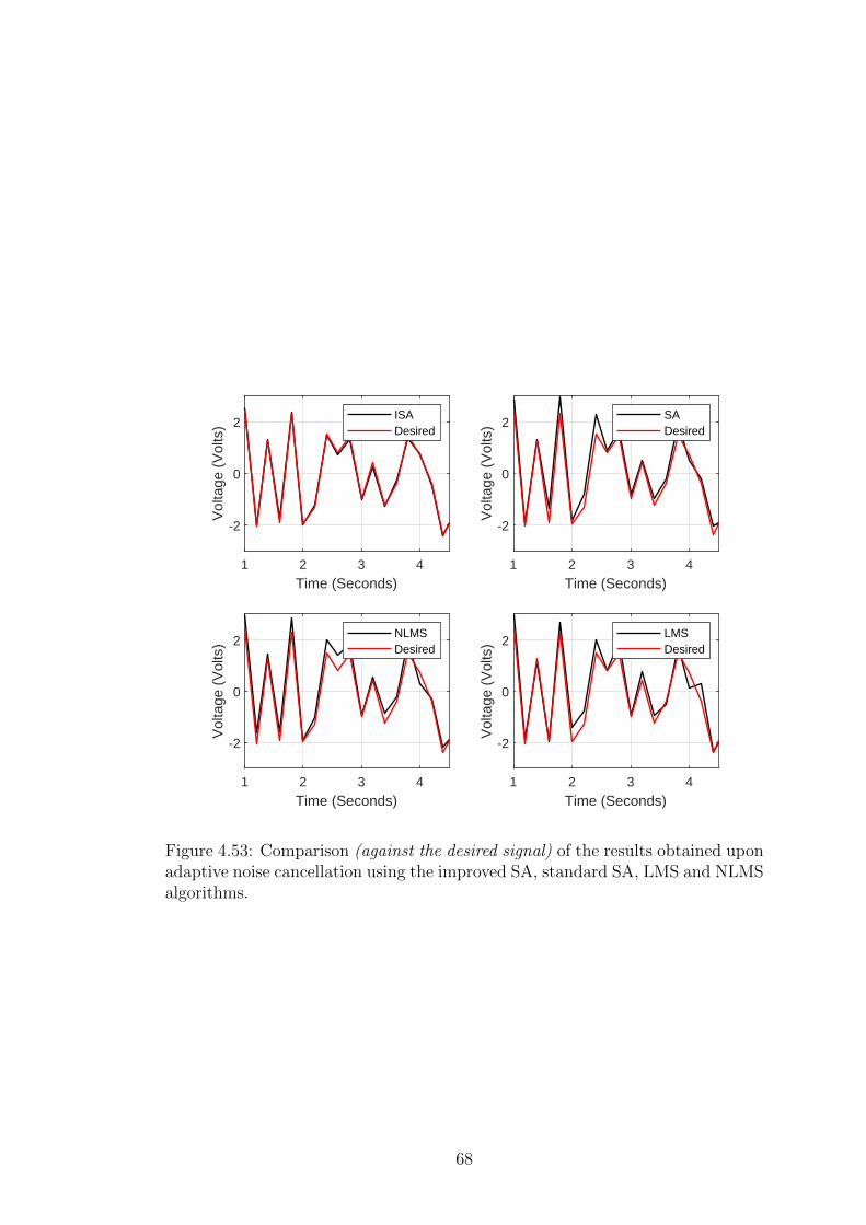
1 2 3 4
Time (Seconds)
-2
0
2
Vol
tage
(V
olts
)
ISADesired
1 2 3 4
Time (Seconds)
-2
0
2
Vol
tage
(V
olts
)
SADesired
1 2 3 4
Time (Seconds)
-2
0
2
Vol
tage
(V
olts
)
NLMSDesired
1 2 3 4
Time (Seconds)
-2
0
2
Vol
tage
(V
olts
)
LMSDesired
Figure 4.53: Comparison (against the desired signal) of the results obtained uponadaptive noise cancellation using the improved SA, standard SA, LMS and NLMSalgorithms.
68
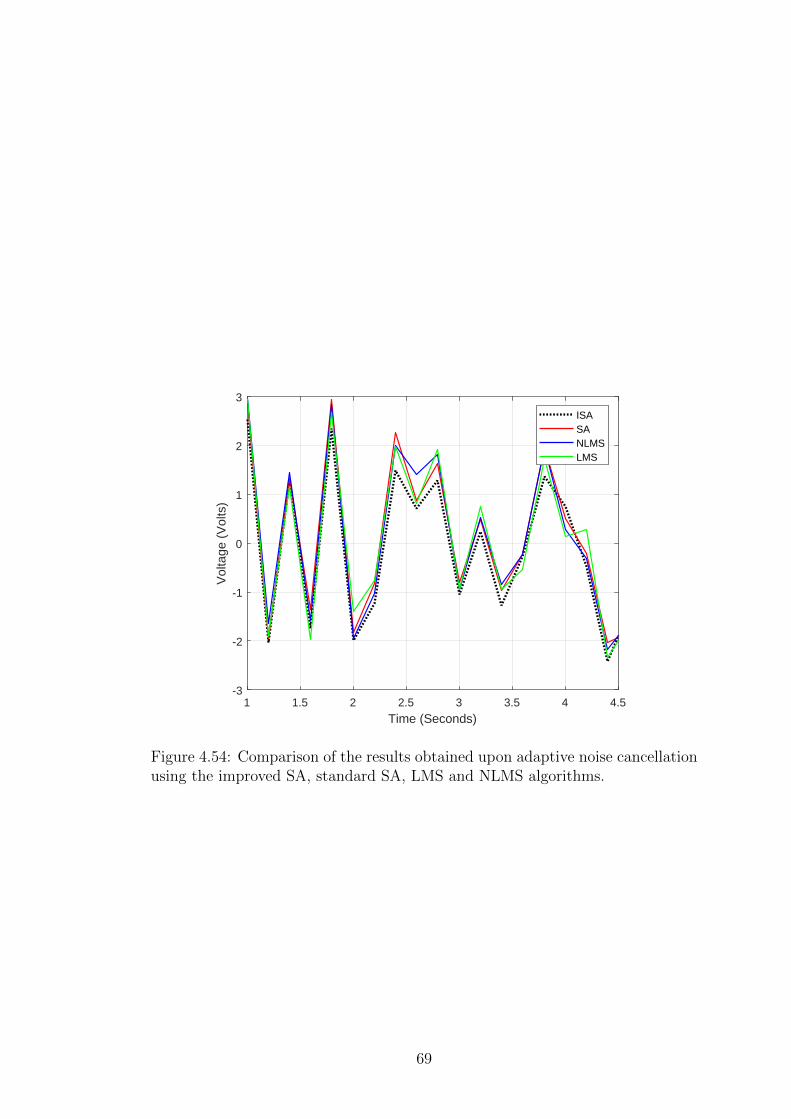
1 1.5 2 2.5 3 3.5 4 4.5
Time (Seconds)
-3
-2
-1
0
1
2
3
Vol
tage
(V
olts
)
ISASANLMSLMS
Figure 4.54: Comparison of the results obtained upon adaptive noise cancellationusing the improved SA, standard SA, LMS and NLMS algorithms.
69
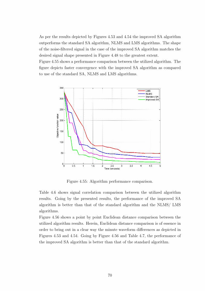
As per the results depicted by Figures 4.53 and 4.54 the improved SA algorithm
outperforms the standard SA algorithm, NLMS and LMS algorithms. The shape
of the noise-filtered signal in the case of the improved SA algorithm matches the
desired signal shape presented in Figure 4.48 to the greatest extent.
Figure 4.55 shows a performance comparison between the utilized algorithm. The
figure depicts faster convergence with the improved SA algorithm as compared
to use of the standard SA, NLMS and LMS algorithms.
Figure 4.55: Algorithm performance comparison.
Table 4.6 shows signal correlation comparison between the utilized algorithm
results. Going by the presented results, the performance of the improved SA
algorithm is better than that of the standard algorithm and the NLMS/ LMS
algorithms.
Figure 4.56 shows a point by point Euclidean distance comparison between the
utilized algorithm results. Herein, Euclidean distance comparison is of essence in
order to bring out in a clear way the minute waveform differences as depicted in
Figures 4.53 and 4.54. Going by Figure 4.56 and Table 4.7, the performance of
the improved SA algorithm is better than that of the standard algorithm.
70
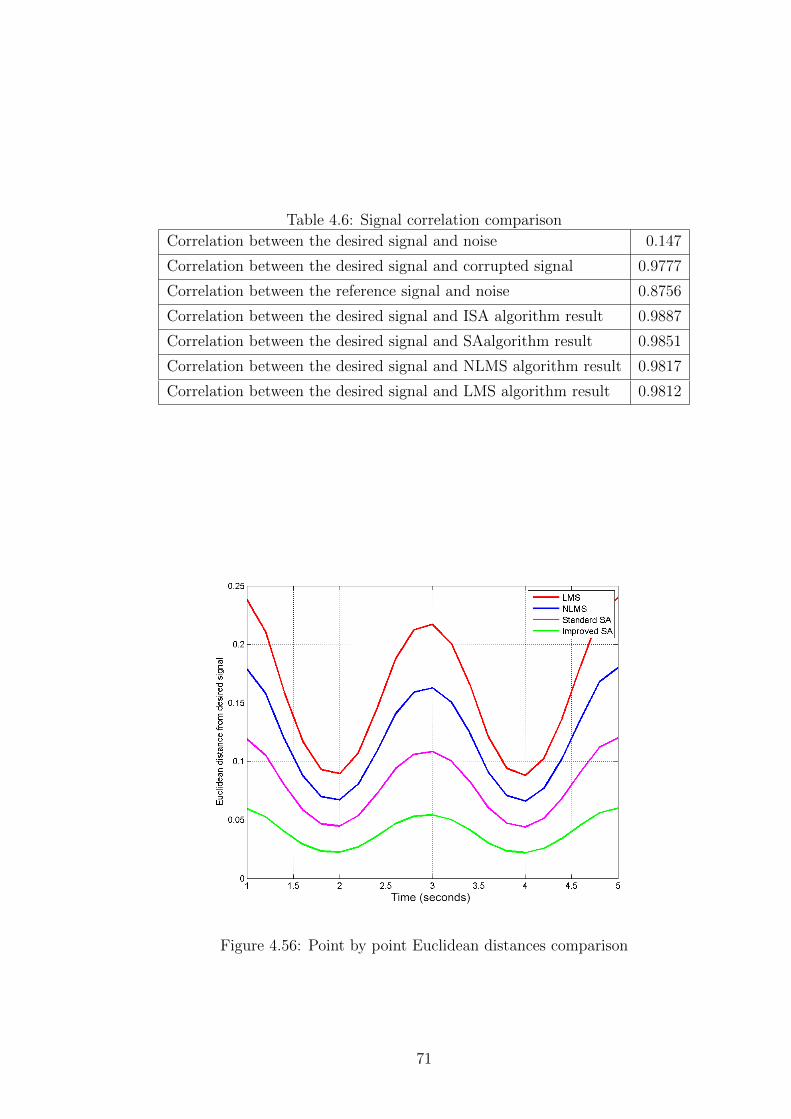
Table 4.6: Signal correlation comparison
Correlation between the desired signal and noise 0.147
Correlation between the desired signal and corrupted signal 0.9777
Correlation between the reference signal and noise 0.8756
Correlation between the desired signal and ISA algorithm result 0.9887
Correlation between the desired signal and SAalgorithm result 0.9851
Correlation between the desired signal and NLMS algorithm result 0.9817
Correlation between the desired signal and LMS algorithm result 0.9812
Figure 4.56: Point by point Euclidean distances comparison
71

Table 4.7: Iregular waveform Euclidean distance comparison
Average Euclidean distance (Improved SA) 0.0401
Average Euclidean distance (SA) 0.0793
Average Euclidean distance (NLMS) 0.1187
Average Euclidean distance (LMS) 0.1546
Discussion
The corrupted waveform and the desired waveform correlation value is 0.9777.
The improved SA result and the desired waveform correlation value is 0.9887.
The standard SA result and the desired waveform correlation value is 0.9851.
The NLMS result and the desired waveform correlation value is 0.9817. The
LMS result and the desired waveform correlation value is 0.9812.
The improved SA algorithm is found to generate better results than the standard
SA algorithm, NLMS algorithm and LMS algorithm in the simulated scenarios.
Generated signal graphs and the corresponding correlation values show that the
improved SA algorithm yields a less noise corrupted signal.
4.2.3 Electrocardiogram waveform
The signal depicted in Figure 4.57 (fetal electrocardiogram signal) is utilized as
the desired signal in the third set of simulations.
The noise signal is depicted in Figure 4.58. The noise signal is composed of
maternal heartbeat and sinusoidal noise.
The noise corrupted signal is depicted in Figure 4.59. The noise signal is composed
of maternal heartbeat and sinusoidal noise.
72
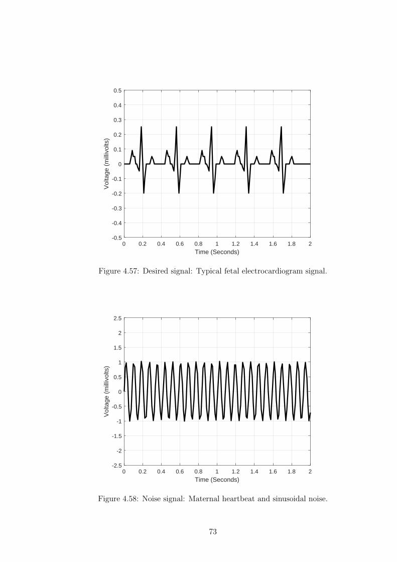
0 0.2 0.4 0.6 0.8 1 1.2 1.4 1.6 1.8 2
Time (Seconds)
-0.5
-0.4
-0.3
-0.2
-0.1
0
0.1
0.2
0.3
0.4
0.5
Vol
tage
(m
illiv
olts
)
Figure 4.57: Desired signal: Typical fetal electrocardiogram signal.
0 0.2 0.4 0.6 0.8 1 1.2 1.4 1.6 1.8 2
Time (Seconds)
-2.5
-2
-1.5
-1
-0.5
0
0.5
1
1.5
2
2.5
Vol
tage
(m
illiv
olts
)
Figure 4.58: Noise signal: Maternal heartbeat and sinusoidal noise.
73

0 0.2 0.4 0.6 0.8 1 1.2 1.4 1.6 1.8 2
Time (Seconds)
-2.5
-2
-1.5
-1
-0.5
0
0.5
1
1.5
2
2.5
Vol
tage
(m
illiv
olts
)
Figure 4.59: Noise corrupted fetal electrocardiogram signal.
The reference signal utilized in the adaptation process is depicted in Figure 4.60.
0 0.2 0.4 0.6 0.8 1 1.2 1.4 1.6 1.8 2
Time (Seconds)
-2.5
-2
-1.5
-1
-0.5
0
0.5
1
1.5
2
2.5
Vol
tage
(m
illiv
olts
)
Figure 4.60: Reference signal (highly correlated to the noise signal).
A comparison of the noise and the reference signals is depicted in Figure 4.61.
74

0 0.2 0.4 0.6 0.8 1 1.2 1.4 1.6 1.8 2
Time (Seconds)
-2.5
-2
-1.5
-1
-0.5
0
0.5
1
1.5
2
2.5
Vol
tage
(m
illiv
olts
)
NoiseReference
Figure 4.61: A comparison of the reference and noise signals.
The results obtained using the improved SA, standard SA, LMS and NLMS al-
gorithms are depicted in Figures 4.62 and 4.63.
75
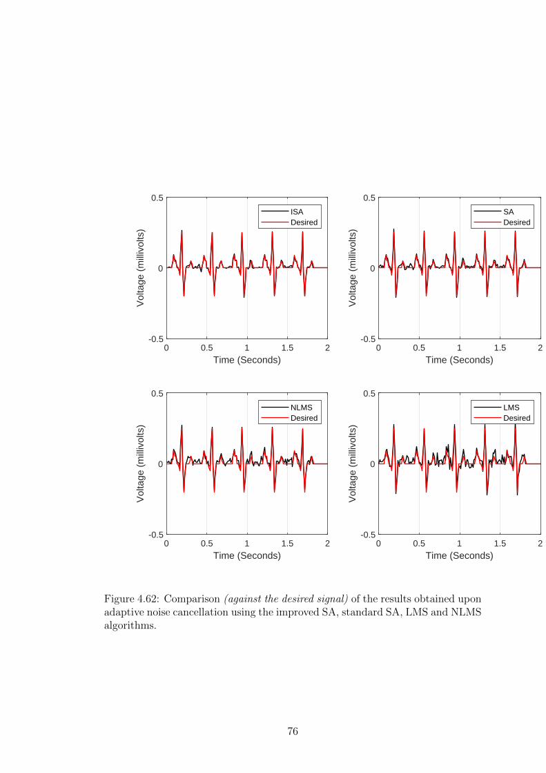
0 0.5 1 1.5 2Time (Seconds)
-0.5
0
0.5
Vol
tage
(m
illiv
olts
)
ISADesired
0 0.5 1 1.5 2Time (Seconds)
-0.5
0
0.5
Vol
tage
(m
illiv
olts
)
SADesired
0 0.5 1 1.5 2Time (Seconds)
-0.5
0
0.5
Vol
tage
(m
illiv
olts
)
NLMSDesired
0 0.5 1 1.5 2Time (Seconds)
-0.5
0
0.5
Vol
tage
(m
illiv
olts
)
LMSDesired
Figure 4.62: Comparison (against the desired signal) of the results obtained uponadaptive noise cancellation using the improved SA, standard SA, LMS and NLMSalgorithms.
76

0 0.2 0.4 0.6 0.8 1 1.2 1.4 1.6 1.8 2
Time (Seconds)
-0.5
-0.4
-0.3
-0.2
-0.1
0
0.1
0.2
0.3
0.4
0.5
Vol
tage
(m
illiv
olts
)
ISASANLMSLMS
Figure 4.63: Comparison of the results obtained upon adaptive noise cancellationusing the improved SA, standard SA, LMS and NLMS algorithms.
77
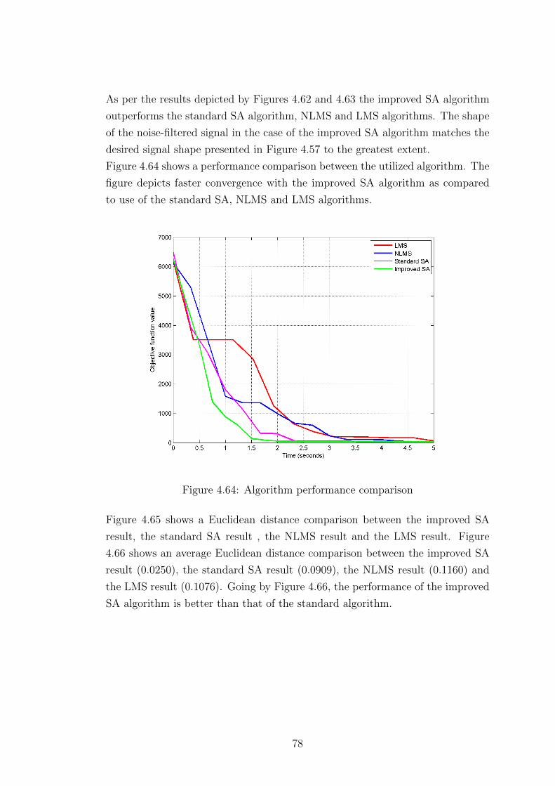
As per the results depicted by Figures 4.62 and 4.63 the improved SA algorithm
outperforms the standard SA algorithm, NLMS and LMS algorithms. The shape
of the noise-filtered signal in the case of the improved SA algorithm matches the
desired signal shape presented in Figure 4.57 to the greatest extent.
Figure 4.64 shows a performance comparison between the utilized algorithm. The
figure depicts faster convergence with the improved SA algorithm as compared
to use of the standard SA, NLMS and LMS algorithms.
Figure 4.64: Algorithm performance comparison
Figure 4.65 shows a Euclidean distance comparison between the improved SA
result, the standard SA result , the NLMS result and the LMS result. Figure
4.66 shows an average Euclidean distance comparison between the improved SA
result (0.0250), the standard SA result (0.0909), the NLMS result (0.1160) and
the LMS result (0.1076). Going by Figure 4.66, the performance of the improved
SA algorithm is better than that of the standard algorithm.
78
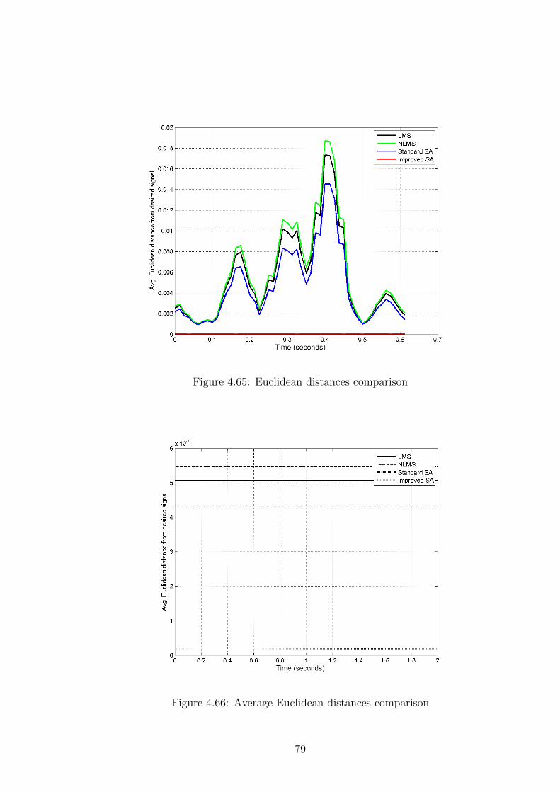
Figure 4.65: Euclidean distances comparison
Figure 4.66: Average Euclidean distances comparison
79
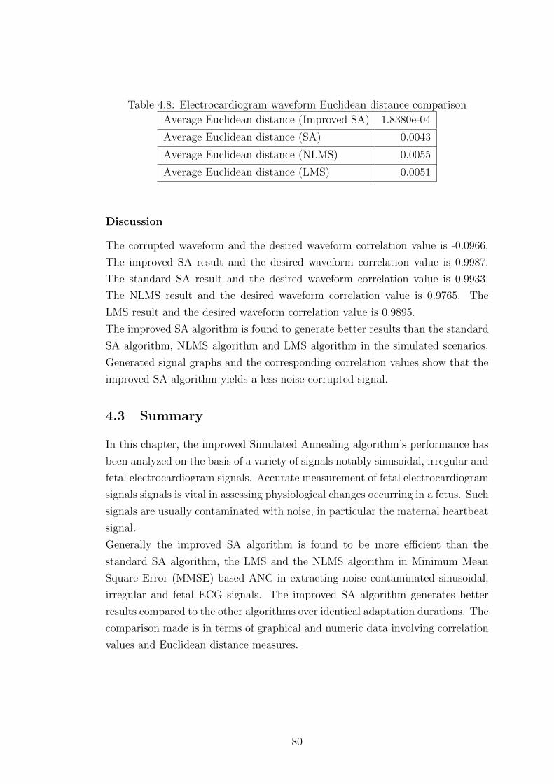
Table 4.8: Electrocardiogram waveform Euclidean distance comparison
Average Euclidean distance (Improved SA) 1.8380e-04
Average Euclidean distance (SA) 0.0043
Average Euclidean distance (NLMS) 0.0055
Average Euclidean distance (LMS) 0.0051
Discussion
The corrupted waveform and the desired waveform correlation value is -0.0966.
The improved SA result and the desired waveform correlation value is 0.9987.
The standard SA result and the desired waveform correlation value is 0.9933.
The NLMS result and the desired waveform correlation value is 0.9765. The
LMS result and the desired waveform correlation value is 0.9895.
The improved SA algorithm is found to generate better results than the standard
SA algorithm, NLMS algorithm and LMS algorithm in the simulated scenarios.
Generated signal graphs and the corresponding correlation values show that the
improved SA algorithm yields a less noise corrupted signal.
4.3 Summary
In this chapter, the improved Simulated Annealing algorithm’s performance has
been analyzed on the basis of a variety of signals notably sinusoidal, irregular and
fetal electrocardiogram signals. Accurate measurement of fetal electrocardiogram
signals signals is vital in assessing physiological changes occurring in a fetus. Such
signals are usually contaminated with noise, in particular the maternal heartbeat
signal.
Generally the improved SA algorithm is found to be more efficient than the
standard SA algorithm, the LMS and the NLMS algorithm in Minimum Mean
Square Error (MMSE) based ANC in extracting noise contaminated sinusoidal,
irregular and fetal ECG signals. The improved SA algorithm generates better
results compared to the other algorithms over identical adaptation durations. The
comparison made is in terms of graphical and numeric data involving correlation
values and Euclidean distance measures.
80
CHAPTER FIVE
CONCLUSION AND RECOMMENDATIONS
5.1 Conclusion
Noise contamination is a common occurrence upon signal transmission through a
noisy channel. Adaptive Noise Cancellation (ANC) is vital in extracting signals
from some noise corrupted signal in a receiver. In this study, ANC in a variety of
signal models typical of signals encountered in communication channels has been
considered.
5.1.1 Highlights and deductions
In particular, the following listing gives the highlights/ deductions made in the
work carried out.
1. An ANC model has been developed in Matlab. The modeled signals include:
sinusoidal signals, fetal electrocardiogram signals and a set of randomly
generated signals.
2. An improved SA algorithm has been developed on the basis of making mod-
ifications to the control parameters of the standard SA. In particular, the
acceptance probability and the cooling schedule procedures have been ad-
justed. An analysis on the acceptance probability and the cooling schedule
procedures relays the superiority of the measures taken towards improving
the SA algorithm.
3. The conventional algorithms utilized in ANC namely Least Mean Squares
(LMS) and Normalized Least Mean Squares (NLMS) algorithms have been
employed and comparisons made against Simulated Annealing (SA) algo-
rithm. Generally the improved SA algorithm is found to be more efficient
than the standard SA algorithm, the LMS and the NLMS algorithm in
Minimum Mean Square Error (MMSE) based ANC in extracting noise con-
taminated sinusoidal, irregular and fetal ECG signals. The improved SA
algorithm generates better results compared to the other algorithms over
identical adaptation durations. The comparison made is in terms of graph-
ical and numeric data involving correlation values and Euclidean distance
measures.
SA algorithm major advantage over other non-gradient based methods (such as
Genetic Algorithm, Tabu Search algorithm, Differential Evolution) is an ability to
81

avoid becoming trapped in local minima. This is because the algorithm employs
a random search technique, which not only accepts changes that decrease the
objective function f (assuming a minimization problem), but also some changes
that increase it with some degree of probability. This therefore guarantees that
the SA algorithm performs better than other AI algorithms in optimization prob-
lems thus the choice in Adaptive Noise Cancellation (ANC), the subject of this
research.
5.1.2 Contribution
A worthwhile contribution of this work has been an analysis on the use of the SA
algorithm in ANC involving sinusoidal, irregular and fetal ECG signals. This is
alongside making worthwhile improvements on the standard SA algorithm. The
improvements are on the basis of making modifications to the control parameters
of the standard SA algorithm. In particular, the acceptance probability and
the cooling schedule procedures have been adjusted. Moreover, the improved
SA algorithm offers a practical solution to noise cancellation problems owing to
its inherent low computation complexity. This work lays forward SA algorithm
advantages over other existing weight update algorithms in ANC.
5.2 Recommendations
The proposed improved SA algorithm is an attractive candidate for use in ANC.
This has been confirmed through simulations involving speech, sinusoidal, irreg-
ular and electrocardiogram waveforms.
As such, it is recommended that the following scenarios be studied further to
establish the full potential of the proposed SA algorithm:
� It is advisable to do a practical analysis concerning the application of SA in
ANC. Due to limitations in laboratory facilities, physical implementations
were not possible in this research.
� Further SA algorithm improvements can be considered particularly towards
further reducing computational complexity.
� It has been established that the adopted cooling schedule bears a huge
impact on the overall SA algorithm performance. Further improvements
on the SA algorithm particularly in the cooling schedule structure can be
considered.
82
REFERENCES
Abdelghani, G., Abdelilah, H., Amine, L., Nezha, M., & Said, R. (2015). A
new method for the extraction of fetal electro cardio gram from the depen-
dent abdominal signals using blind source separation and adaptive noise
cancellation techniques. Theoretical Biology and Medical Modelling , 12 (1),
25-35.
Alazamir, S., Rebennack, S., & Pardalos, P. M. (2008, July). Improving the
neighborhood selection strategy in simulated annealing using optimal stop-
ping problem. I-Tech Education and Publication, 10 (1), 363-382.
Albert, S. D. (1991). Fundamentals of adaptive noise cancellation (1st ed.). U.
S. Army Laboratory Command.
Arif, M., Naseem, I., Moinuddin, M., Khan, S. S., & Ammar, M. M. (2017,
April). Adaptive noise cancellation using q-lms. In 2017 international
conference on innovations in electrical engineering and computational tech-
nologies (icieect) (p. 1-4).
Bajic, V. (2005). Design and implementation of an adaptive noise canceling
system in wavelet transform domain (1st ed.). University of Akron.
Balaji, P., Narayan, S., Sraddha, D., & Muthu, R. K. (2020). Performance
analysis of adaptive noise cancellation for speech signal. arXiv preprint
arXiv:2002.07677 .
Bayram, H., & Azahin, R. (2013, January). A new simulated annealing ap-
proach for travelling salesman problem. Mathematical and Computational
Applications , 18 (3), 313-322.
Bellanger, M. G. (2001). Adaptive digital filters (2nd ed.). Marcel Dekker.
Bezakova, I., Stefankovi, D., Vazirani, V. V., & Vigoda, E. (2006, July). Accel-
erating simulated annealing for the permanent and combinatorial counting
problems. Proceedings of the 17th Annual ACM-SIAM Symposium on Dis-
crete Algorithms , 10 (1), 900-907.
Bisht, S. (2004, July). Hybrid genetic-simulated annealing algorithm for optimal
83
weapon allocation in multilayer defence scenario. Defence Science Journal ,
54 (3), 395-405.
Busetti, F. (2005). Simulated annealing overview (1st ed.). JP Morgan.
Chang, C.-Y., & Chen, D.-R. (2010). Active noise cancellation without sec-
ondary path identification by using an adaptive genetic algorithm. IEEE
Transactions on Instrumentation and Measurement , 59 (9), 2315-2327.
Dewangan, N., & M., P. R. (2014). Noise cancellation using adaptive filter
for phonocardiogram signal. International journal of emerging trends and
technology in computer science, 3 (4), 38-43.
Dimitris, B., & Tsitsiklls, J. (1993). Simulated annealing. Statistical Science,
8 (1), 10-15.
Dixit, S., & Nagaria, D. (2019). Hardware reduction in cascaded lms adaptive
filter for noise cancellation using feedback. Circuits, Systems, and Signal
Processing , 38 (2), 930-945.
Emile, A., Jan, K., & Wil, M. (2014). Search methodologies: Introductory tutorials
in optimization and decision support techniques (1st ed.). Springer.
Ferreiro, A. M., A., G. J., G., L.-S. J., & C., V. (2013). An efficient implementa-
tion of parallel simulated annealing algorithm in general processing units.
Journal of Global Optimization, 57 (3), 863-890.
Garcia, E., Marcela, L., & Araiza, G. (2012, July). Simulated annealing with pre-
vious solutions applied to deoxyribonucleic acid sequence alignment. ISRN
Artificial Intelligence, 12 (1), 1-7.
Ghodsi, M., Hassani, H., & Sanei, S. (2010, January). Extracting fetal heart
signal from noisy maternal ecg by multivariate singular spectrum analysis.
Statistics and Its Interface, 3 , 399-411.
Hameed, A. A. (2012). Real-time noise cancellation using adaptive algorithms
(1st ed.). Eastern Mediterranean University.
84
Haykin, S. (2002). Adaptive filter theory (4th ed.). Prentice Hall.
Jatoth, R. K. (2006, May). An intelligent adaptive noise cancellation system for
the extraction of fetal electrocardiogram. Proceedings of the WSEAS In-
ternational Conference on signal processing, robotics and automation, 1 (1),
193-197.
Kang, L., & Zhu, X. (2016). A simulated annealing algorithm for first train trans-
fer problem in urban railway networks. Applied Mathematical Modelling ,
40 (1), 419-435.
Kapoor, J., Mishra, G., & Rai, M. (2017, Nov). Characteristics and properties
of audio signal and noise cancellation techniques: A theoretical review. In
2017 international conference on emerging trends in computing and com-
munication technologies (icetcct) (p. 1-4).
Li, L., Xu, W., Hong, Q., Tong, F., & Wu, J. (2016). Adaptive noise cancel-
lation and classification of lung sounds under practical environment. 2016
10th IEEE International Conference on Anti-counterfeiting, Security, and
Identification (ASID), 39-42.
Li, Y., Guo, H., Wang, L., & Fu, J. (2013). A hybrid genetic-simulated annealing
algorithm for the location-inventory-routing problem considering returns
under e-supply chain environment. The Scientific World Journal , 2013 .
Ludger, S. (2015, February). Adaptive noise cancellation for multi-
microphone systems (Tech. Rep.). Google Patents. Retrieved from
https://www.google.com/patents/US8958572
Mahdi, W., Medjahed, S. A., & Ouali, M. (2017). Performance analysis of simu-
lated annealing cooling schedules in the context of dense image matching.
Computacion y Sistemas , 21 (3), 493-501.
Martinek, R., Kelnar, M., Vanus, J., Koudelka, P., Bilik, P., Koziorek, J., &
Zidek, J. (2015). Adaptive noise suppression in voice communication using
a neuro-fuzzy inference system. 2015 38th International Conference on
Telecommunications and Signal Processing (TSP), 382-386.
85
Maurya, A. K., Agrawal, P., & Dixit, S. (2019). Modified model and algorithm
of lms adaptive filter for noise cancellation. Circuits, Systems, and Signal
Processing , 38 (5), 2351-2368.
Mehmood, H. S., Ahmad, R. Z., & Yousuf, M. J. (2019). A comprehensive
review of adaptive noise cancellation techniques in the internet of things.
In Proceedings of the 3rd international conference on future networks and
distributed systems (p. 1-8).
Miyahara, R., Oosugi, K., & Sugiyama, A. (2019). A hearing device with an
adaptive noise canceller for noise-robust voice input. IEEE Transactions
on Consumer Electronics , 65 (4), 444-453.
Munjuluri, L., Preetam, R. M., Rakesh, T., Gopi, K., & L, B. K. V. (2015).
An insight into adaptive noise cancellation and comparison of algorithms.
Journal of Theoretical and Applied Information Technology , 79 (1), 57-64.
Murugendrappa, N., Ananth, A., & Mohanesh, K. (2020). Adaptive noise can-
cellation using kalman filter for non-stationary signals. In Iop conference
series: Materials science and engineering (Vol. 925, p. 012-061).
Nouri, B. V., Fattahi, P., & Ramezanian, R. (2013). Hybrid firefly-simulated an-
nealing algorithm for the flow shop problem with learning effects and flex-
ible maintenance activities. International Journal of Production Research,
51 (12), 3501-3515.
Patnaik, A., Patjoshi, R. K., & Panigrahi, R. (2020). An experimental inves-
tigation of fpga-based lms algorithm for adaptive noise cancellation. In
Electronic systems and intelligent computing (p. 719-730). Springer.
Patrick, S. K., Gelatt, C. D., & Vecchi, M. P. (1983). Optimization by simulated
annealing. Journal of Science, 220 (4598), 671-680.
Pitchaiah, T., Sridevi, P. V., & Rao, S. K. (2015). Adaptive noise cancella-
tion using least mean squares algorithm in monte carlo simulation. 2015
2nd International Conference on Electronics and Communication Systems
(ICECS), 368-372.
86

Shang, Q., Chen, L., & Peng, P. (2020). On-chip evolution of combinational logic
circuits using an improved genetic-simulated annealing algorithm. Concur-
rency and Computation: Practice and Experience, 32 (23), 54-86.
Shi, L., Zhao, H., Wang, W., & Lu, L. (2019). Combined regularization pa-
rameter for normalized lms algorithm and its performance analysis. Signal
Processing , 162 , 75-82.
Shiva, G. B., Anwar, F., Brian, H., & Hilmi, D. (2016). Neural network-based
adaptive noise cancellation for enhancement of speech auditory brainstem
responses. Signal, Image and Video Processing , 10 (2), 389-395.
Shubhra, D., & Deepak, N. (2014). Neural network implementation of least-mean-
square adaptive noise cancellation. 2014 International Conference on Issues
and Challenges in Intelligent Computing Techniques (ICICT), 134-139.
Singh, A. (2001). Adaptive noise cancellation (1st ed.). Netaji Subhas Institute
of Technology.
Singh, G., Savita, K., & Yadav, S. (2013, May). Design of adaptive noise canceller
using lms algorithm. IJATER, 3 (1), 85-89.
Tanaka, Y., Izumi, S., Kawamoto, Y., Kawaguchi, H., & Yoshimoto, M. (2016).
Adaptive noise cancellation method for capacitively coupled ecg sensor us-
ing single insulated electrode. 2016 IEEE Biomedical Circuits and Systems
Conference (BioCAS), 296-299.
Thakur, R., Dutta, P., & Manna, D. G. (2014). Analysis and comparison of
evolutionary algorithms applied to adaptive noise cancellation for speech
signal. International Journal of Recent Development in Engineering and
Technology , 3 (1), 172-178.
Thunga, S. S., & Muthu, R. K. (2020). Adaptive noise cancellation using im-
proved lms algorithm. In Soft computing for problem solving (p. 971-980).
Springer.
Tsao, Y., Chu, H., Fang, S., Lee, J., & Lin, C. (2018). Adaptive noise cancellation
87
using deep cerebellar model articulation controller. IEEE Access , 6 , 37395-
37402.
Wei, H., & Shao, L. (2019). Combination of lms algorithm in adaptive noise
cancellation system. In Iop conference series: Materials science and engi-
neering (Vol. 677, p. 2-22).
Widrow, B. (1975, December). Adaptive noise cancelling: principles and appli-
cations. Proc. of the IEEE , 63 (12), 1692-1716.
Wu, G., Wang, H., Pedrycz, W., Li, H., & Wang, L. (2017). Satellite observation
scheduling with a novel adaptive simulated annealing algorithm and a dy-
namic task clustering strategy. Computers & Industrial Engineering , 113 ,
576-588.
Xia, L., Hui, G., & Jinfeng, L. (2008). Adaptive noise canceller based on pso
algorithm. In 2008 ieee international conference on automation and logistics
(p. 1759-1762).
Xu, M., Li, S., & Guo, J. (2017). Optimization of multiple traveling salesman
problem based on simulated annealing genetic algorithm. In Matec web of
conferences (Vol. 100, p. 20-25).
Yang, D., Cheng, Y., Zhu, J., Xue, D., Abt, G., Ye, H., & Peng, Y. (2018). A novel
adaptive spectrum noise cancellation approach for enhancing heartbeat rate
monitoring in a wearable device. IEEE Access , 6 , 8364-8375.
Yang, Z.-K., Shi, H., Zhao, S., & Huang, X.-D. (2020). Vital sign detection during
large-scale and fast body movements based on an adaptive noise cancellation
algorithm using a single doppler radar sensor. Sensors , 20 (15), 41-83.
Yannibelli, V., & Amandi, A. (2013). Hybridizing a multi-objective simulated
annealing algorithm with a multi-objective evolutionary algorithm to solve
a multi-objective project scheduling problem. Expert Systems with Appli-
cations , 40 (7), 2421-2434.
Yao, X. (2008). Dynamic neighbourhood size in simulated annealing (1st ed.).
88
Australian Defence Force Academy.
Yelwande, A., Kansal, S., & Dixit, A. (2017, Aug). Adaptive wiener filter for
speech enhancement. In 2017 international conference on information, com-
munication, instrumentation and control (icicic) (p. 1-4).
Zhang, C., Wang, H., Jiang, Y., & Chen, X. (2017). Application of improved
simulated annealing algorithm in tsp. Computer engineering and software.
Zhou, X., & Shao, Y. (2014). Adaptive noise cancellation based on beehive pat-
tern evolutionary digital filter. Mechanical Systems and Signal Processing ,
42 (1-2), 225-235.
89
APPENDICES
Appendix 1: Published Work
The following papers arising from the research work have been published:
1. Kevin Mwongera, Kibet Lang’at, and E. N. Ndung’u: Design of adaptive noise
canceler in speech signals using simulated annealing algorithm. (Proceedings of
SIR conference, 2015) In this paper, use of the simulated annealing algorithm in
adaptive noise cancelation in speech signals is studied. A comparison is made
between use of the simulated annealing algorithm and the commonly used Least
Mean Squares (LMS) algorithm. The simulated annealing algorithm is found to
perform better than the LMS algorithm. The entire analysis is made through
simulations in Matlab software.
2. Kevin Mwongera, Kibet Lang’at, and E. N. Ndung’u: Design of adaptive noise
canceler in fetal electrocardiogram signal extraction using simulated annealing
algorithm. (Proceedings of SIR conference, 2015) This paper analyzes use of
adaptive noise canceling techniques in filtering noisy FECG using simulated an-
nealing algorithm. A comparison is made between use of the simulated annealing
algorithm and the commonly used Least Mean Squares (LMS) algorithm. Ob-
tained correlation values are used as the performance measure. The simulated
annealing algorithm is found to perform better than the LMS algorithm. The
entire analysis is made through simulations in Matlab software.
3. K. Mwongera, K. Lang’at, and E. N. Ndung’u: Fetal Heartbeat Signal Extrac-
tion using an Adaptive Noise Canceller implemented with an improved Simulated
Annealing Algorithm. (IOSR -JVSP Journal vol 7 issue 5, 2017) In this paper,
an improved Simulated Annealing (SA) algorithm is utilized in ANC to yield a
minimal-noise fetal electrocardiogram signal through simulations done in MAT-
LAB. A performance analysis between use of the improved SA algorithm and
the standard SA algorithm (alongside Genetic, Least Mean Squares (LMS) and
Normalized Least Mean Squares (NLMS) algorithms) is done.On the basis of con-
vergence rate and final solution accuracy the improved SA algorithm performance
is found to outweigh the other algorithms considered in the study.
90
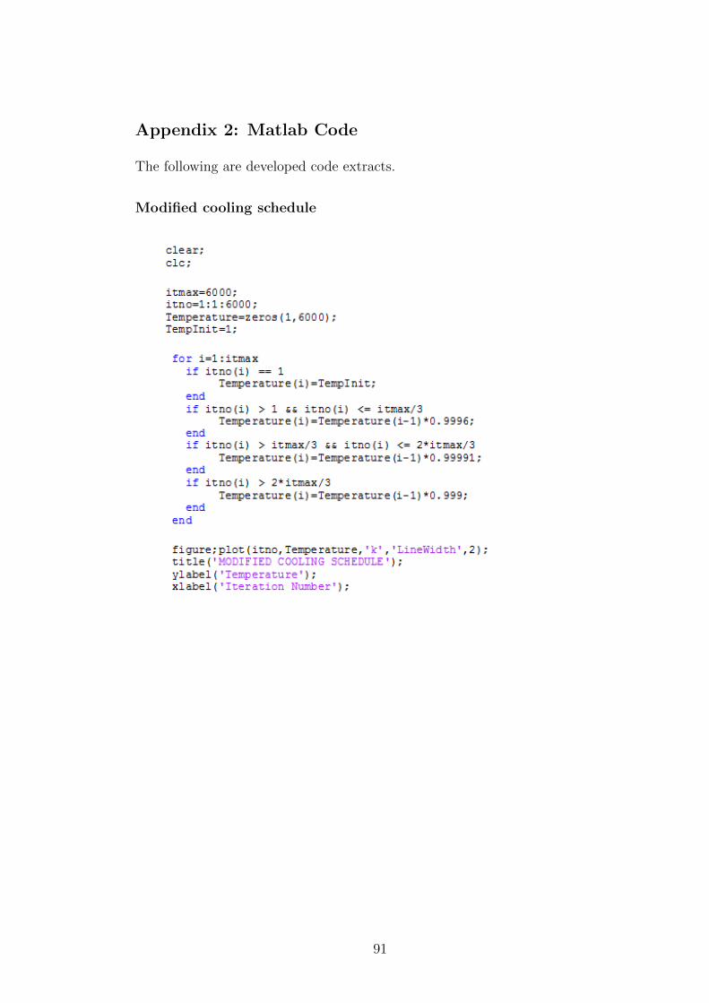
Appendix 2: Matlab Code
The following are developed code extracts.
Modified cooling schedule
91
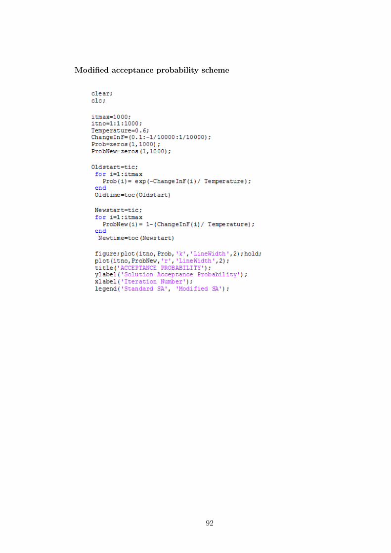
Modified acceptance probability scheme
92
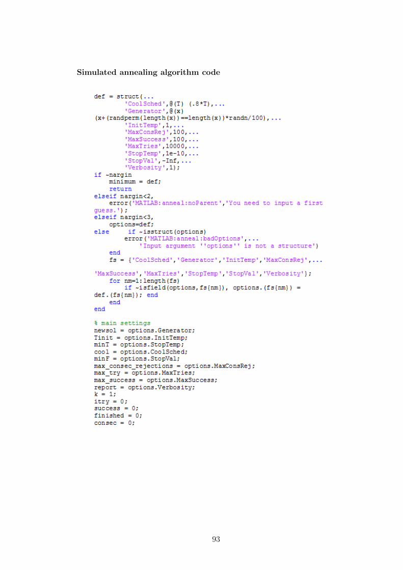
Simulated annealing algorithm code
93
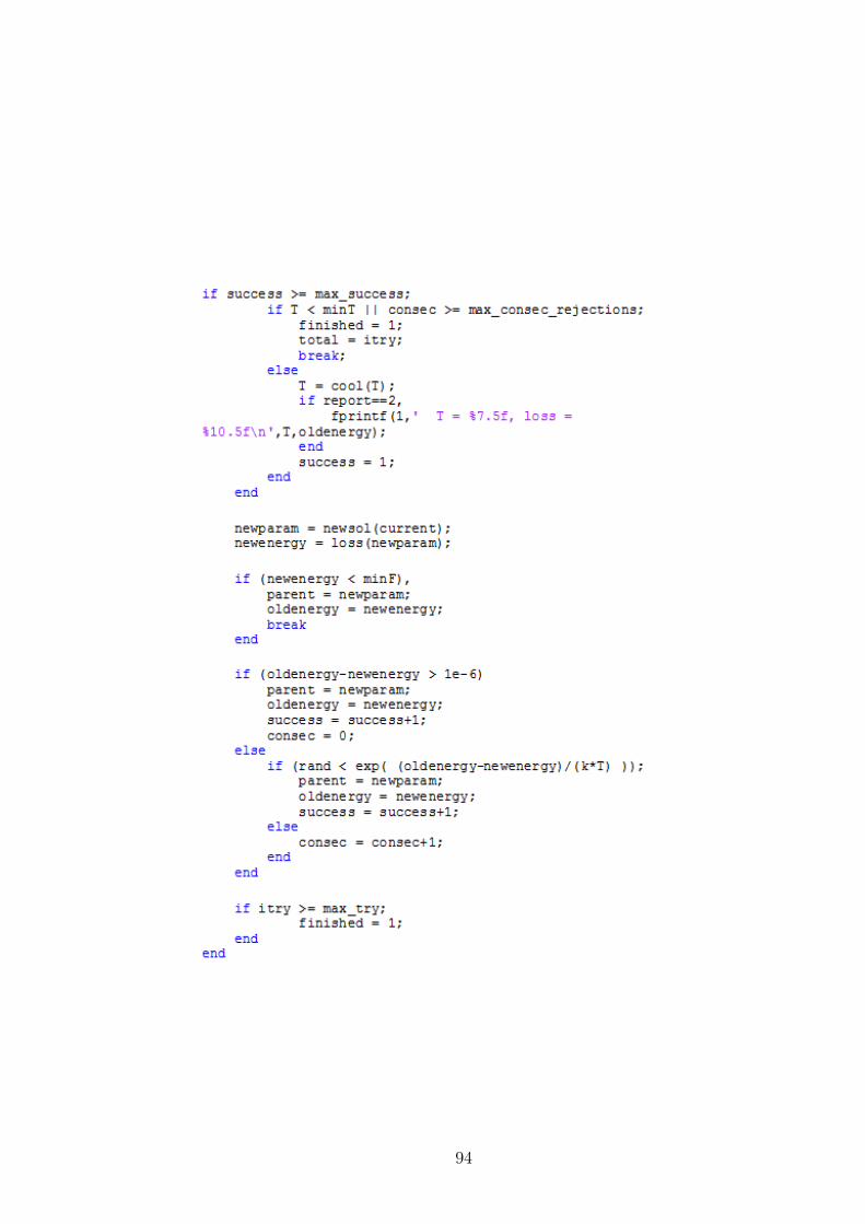
94
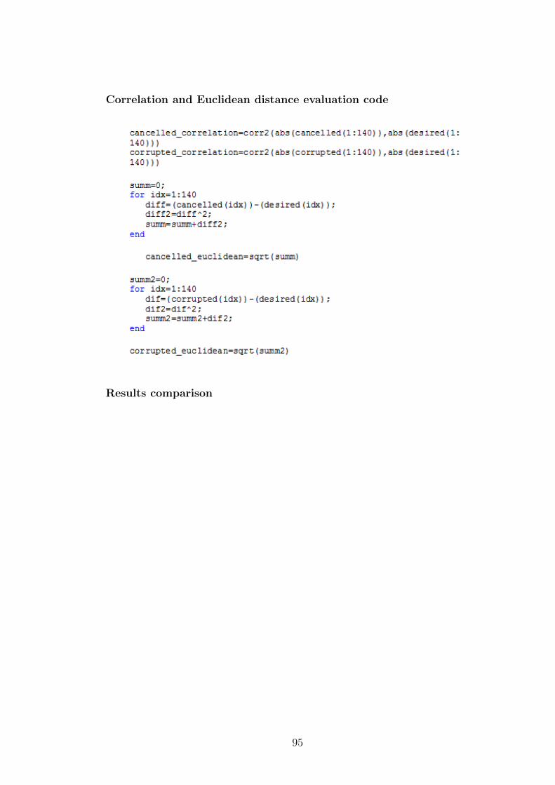
Correlation and Euclidean distance evaluation code
Results comparison
95
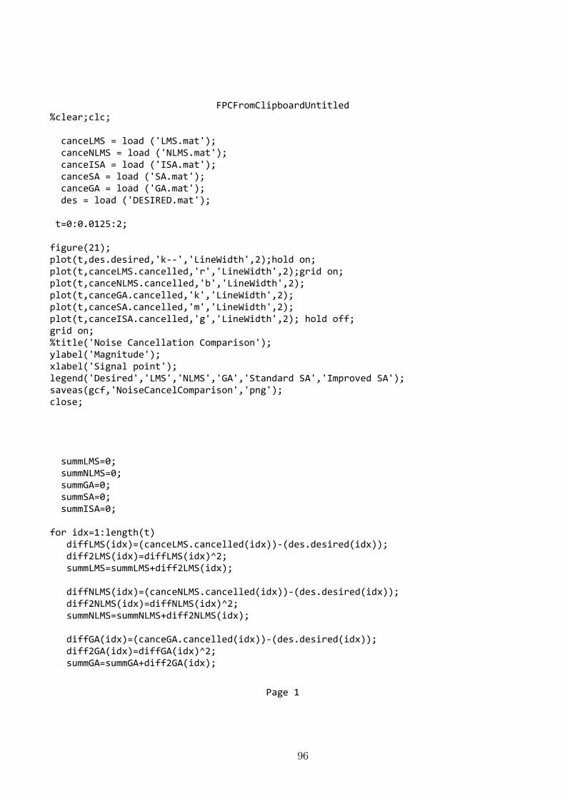
FPCFromClipboardUntitled%clear;clc;
canceLMS = load ('LMS.mat'); canceNLMS = load ('NLMS.mat'); canceISA = load ('ISA.mat'); canceSA = load ('SA.mat'); canceGA = load ('GA.mat'); des = load ('DESIRED.mat');
t=0:0.0125:2;
figure(21);plot(t,des.desired,'k--','LineWidth',2);hold on;plot(t,canceLMS.cancelled,'r','LineWidth',2);grid on;plot(t,canceNLMS.cancelled,'b','LineWidth',2);plot(t,canceGA.cancelled,'k','LineWidth',2);plot(t,canceSA.cancelled,'m','LineWidth',2);plot(t,canceISA.cancelled,'g','LineWidth',2); hold off;grid on;%title('Noise Cancellation Comparison');ylabel('Magnitude');xlabel('Signal point');legend('Desired','LMS','NLMS','GA','Standard SA','Improved SA');saveas(gcf,'NoiseCancelComparison','png');close;
summLMS=0; summNLMS=0; summGA=0; summSA=0; summISA=0;
for idx=1:length(t) diffLMS(idx)=(canceLMS.cancelled(idx))-(des.desired(idx)); diff2LMS(idx)=diffLMS(idx)^2; summLMS=summLMS+diff2LMS(idx);
diffNLMS(idx)=(canceNLMS.cancelled(idx))-(des.desired(idx)); diff2NLMS(idx)=diffNLMS(idx)^2; summNLMS=summNLMS+diff2NLMS(idx);
diffGA(idx)=(canceGA.cancelled(idx))-(des.desired(idx)); diff2GA(idx)=diffGA(idx)^2; summGA=summGA+diff2GA(idx);
Page 1
96
FPCFromClipboardUntitled diffSA(idx)=(canceSA.cancelled(idx))-(des.desired(idx)); diff2SA(idx)=diffSA(idx)^2; summSA=summSA+diff2SA(idx);
diffISA(idx)=(canceISA.cancelled(idx))-(des.desired(idx)); diff2ISA(idx)=diffISA(idx)^2; summISA=summISA+diff2ISA(idx);end
euclideanLMS=sqrt(diff2LMS); SUMeuclideanLMS=sqrt(summLMS)
euclideanNLMS=sqrt(diff2NLMS); SUMeuclideanNLMS=sqrt(summNLMS)
euclideanGA=sqrt(diff2GA); SUMeuclideanGA=sqrt(summGA)
euclideanSA=sqrt(diff2SA); SUMeuclideanSA=sqrt(summSA)
euclideanISA=sqrt(diff2ISA); SUMeuclideanISA=sqrt(summISA)
figure;plot(t,euclideanLMS,'r','LineWidth',2);hold on; plot(t,euclideanNLMS,'b','LineWidth',2);grid on; plot(t,euclideanGA,'k-','LineWidth',2); plot(t,euclideanSA,'m','LineWidth',2); plot(t,euclideanISA,'g','LineWidth',2); hold off; grid on; %title('Euclidean distance from desired signal'); ylabel('Magnitude'); xlabel('Signal point'); legend('LMS','NLMS','GA','Standard SA','Improved SA'); saveas(gcf,'EuclidCompare','png'); close;
for idx=1:length(t) OverallLMS(idx)=SUMeuclideanLMS; OverallNLMS(idx)=SUMeuclideanNLMS; OverallGA(idx)=SUMeuclideanGA; OverallSA(idx)=SUMeuclideanSA; OverallISA(idx)=SUMeuclideanISA;end
Page 2
97
FPCFromClipboardUntitled figure;plot(t,OverallLMS,'r','LineWidth',2);hold on; plot(t,OverallNLMS,'b','LineWidth',2);grid on; plot(t,OverallGA,'k-','LineWidth',2); plot(t,OverallSA,'m','LineWidth',2); plot(t,OverallISA,'g','LineWidth',2); hold off; grid on; %title('Overall euclidean distance from desired signal'); ylabel('Magnitude'); xlabel('Signal point'); legend('LMS','NLMS','GA','Standard SA','Improved SA'); saveas(gcf,'OverallEuclidCompare','png');
Page 3
98
FPCFromClipboardUntitledfigure;load('LMSFitness.mat');plot(GAXdata,GAYdata,'r','LineWidth',2);hold on;load('NLMSFitness.mat');plot(GAXdata,GAYdata,'b','LineWidth',2);load('SAFitness.mat');plot(GAXdata,GAYdata,'m','LineWidth',2);load('ISAFitness.mat');plot(GAXdata,GAYdata,'g','LineWidth',2);title('');xlabel('Iteration'); ylabel('Objective function value');grid on;legend('LMS','NLMS','Standard SA','Improved SA');
%saveas(gcf,'PFitnessComparisonThesis','png');
figure;load('SAFitness.mat');plot(GAXdata,GAYdata,'k','LineWidth',2);hold;load('ISAFitness.mat');plot(GAXdata,GAYdata,'k--','LineWidth',2);title('');xlabel('Iteration'); ylabel('Objective function value');grid on;legend('Standard SA','Improved SA');
%saveas(gcf,'PFitnessComparisonThesis2','png');
figure;load('LMSFitness.mat');GAXdataTime=(5*GAXdata)/max(GAXdata);plot(GAXdataTime,GAYdata,'r','LineWidth',2);hold on;load('NLMSFitness.mat');GAXdataTime=(5*GAXdata)/max(GAXdata);plot(GAXdataTime,GAYdata,'b','LineWidth',2);load('SAFitness.mat');GAXdataTime=(5*GAXdata)/max(GAXdata);plot(GAXdataTime,GAYdata,'m','LineWidth',2);load('ISAFitness.mat');GAXdataTime=(5*GAXdata)/max(GAXdata);plot(GAXdataTime,GAYdata,'g','LineWidth',2);title('');xlabel('Time (seconds)');
Page 1
99
FPCFromClipboardUntitledylabel('Objective function value');grid on;legend('LMS','NLMS','Standard SA','Improved SA');
saveas(gcf,'PFitnessComparisonThesisHE','png');
figure;
load('SAFitness.mat');GAXdataTime=(5*GAXdata)/max(GAXdata);plot(GAXdataTime,GAYdata,'k','LineWidth',2);hold on;load('ISAFitness.mat');GAXdataTime=(5*GAXdata)/max(GAXdata);plot(GAXdataTime,GAYdata,'k--','LineWidth',2);title('');xlabel('Time (seconds)'); ylabel('Objective function value');grid on;legend('Standard SA','Improved SA');
saveas(gcf,'PFitnessComparisonThesis2HE','png');
Page 2
100