ADAPTIVE Klippel, NONLINEAR CONTROL OF LOUDSPEAKER SYSTEMS. · 17 ADAPTIVE NONLINEAR CONTROL OF...
32
17 ADAPTIVE NONLINEAR CONTROL OF LOUDSPEAKER SYSTEMS Wolfgang J. Klippel KLIPPEL GmbH, AussigerStr. 3, 01277 Dresden [email protected] ABSTRACT: Signal distortions caused by loudspeaker nonlinearities can be compensated by inverse nonlinear processing of the electric driving signal. This concept is based on an adequate control architecture having free control parameters adjusted to the particular loudspeaker. Optimal performance requires a self-tuning (adaptive) system to compensate for variations of loudspeaker parameters due to the effect of heating and aging while reproducing the audio signal. Straightforward adaptive controllers use an additional nonlinear filter for modeling the loudspeaker and for transforming the identified parameters into control parameters. This approach is susceptible to systematic errors and can not be implemented in available DSP-systems at low costs. This paper presents a novel technique for direct updating of the control parameters which makes separate system identification superfluous. 1. INTRODUCTION Designing a woofer or a horn compression driver with high acoustic output, maximal efficiency, small dimensions, low weight and manufactured at limited costs we cope with nonlinearities inherent in the transducer which generate audible distortion in the reproduced sound. Although the search for electric means to compensate actively for this distortion has a long history the progress in digital audio opens new perspectives. Novel control architectures [1], [2], [3] have been developed which give better performance than servo control based on negative feedback of a motional signal [4], [5]. However, the free parameters of the new digital controllers must carefully be adjusted to the particular loudspeaker to cancel the distortion in the output signal successfully. In this respect servo control has a clear advantage because it simplifies the adjustment and remains operative for changing loudspeaker parameters due to warming and aging as long as the stability of the feedback loop can be assured. In order obtain the same benefit the new digital controllers need an automatic parameter adjustment performed by the controller itself on reproducing an ordinary audio signal. A system with such a self-learning feature is commonly called adaptive. This paper contributes to the development of adaptive controllers dedicated to loudspeaker systems and is organized in the following way. At the beginning a summary on the results of loudspeaker modeling and the control design is given. From this point of view the known schemes for adaptive control are discussed and novel algorithms are presented. The behavior of the different approaches is investigated by numerical simulations. Finally practical results of a direct adaptive controller implemented on a DSP 56000 are presented and conclusions for the controller design are given.
Transcript of ADAPTIVE Klippel, NONLINEAR CONTROL OF LOUDSPEAKER SYSTEMS. · 17 ADAPTIVE NONLINEAR CONTROL OF...
17
ADAPTIVE NONLINEAR CONTROL OF LOUDSPEAKER
SYSTEMS
Wolfgang J. Klippel
KLIPPEL GmbH, AussigerStr. 3, 01277 Dresden [email protected]
ABSTRACT: Signal distortions caused by loudspeaker nonlinearities can be compensated by inverse nonlinear processing of the electric driving signal. This concept is based on an adequate control architecture having free control parameters adjusted to the particular loudspeaker. Optimal performance requires a self-tuning (adaptive) system to compensate for variations of loudspeaker parameters due to the effect of heating and aging while reproducing the audio signal. Straightforward adaptive controllers use an additional nonlinear filter for modeling the loudspeaker and for transforming the identified parameters into control parameters. This approach is susceptible to systematic errors and can not be implemented in available DSP-systems at low costs. This paper presents a novel technique for direct updating of the control parameters which makes separate system identification superfluous.
1. INTRODUCTION Designing a woofer or a horn compression driver with high acoustic output, maximal efficiency, small dimensions, low weight and manufactured at limited costs we cope with nonlinearities inherent in the transducer which generate audible distortion in the reproduced sound. Although the search for electric means to compensate actively for this distortion has a long history the progress in digital audio opens new perspectives. Novel control architectures [1], [2], [3] have been developed which give better performance than servo control based on negative feedback of a motional signal [4], [5]. However, the free parameters of the new digital controllers must carefully be adjusted to the particular loudspeaker to cancel the distortion in the output signal successfully. In this respect servo control has a clear advantage because it simplifies the adjustment and remains operative for changing loudspeaker parameters due to warming and aging as long as the stability of the feedback loop can be assured. In order obtain the same benefit the new digital controllers need an automatic parameter adjustment performed by the controller itself on reproducing an ordinary audio signal. A system with such a self-learning feature is commonly called adaptive. This paper contributes to the development of adaptive controllers dedicated to loudspeaker systems and is organized in the following way. At the beginning a summary on the results of loudspeaker modeling and the control design is given. From this point of view the known schemes for adaptive control are discussed and novel algorithms are presented. The behavior of the different approaches is investigated by numerical simulations. Finally practical results of a direct adaptive controller implemented on a DSP 56000 are presented and conclusions for the controller design are given.

18
2. PLANT MODELING The basis for the design of a nonlinear controller dedicated to loudspeakers is the development of a precise loudspeaker model considering the dominant nonlinearities. For more than 10 years major efforts have been made to get a better insight into the behavior of loudspeakers at large amplitudes where the linear models fail. The equivalent circuits have been expanded by considering the dependence of parameters on instantaneous quantities (states) of the circuit. In woofer systems, for example, the force factor, the stiffness of the mechanical suspension and the inductance vary with the displacement of the voice coil generating a nonlinear system represented by a nonlinear differential equation. In this paper we use a more general model that abstracts from the physical details of the transducer but preserves the structural information which is important for controller design. Taking the time-discrete voltage u(i) at the terminals as the loudspeaker input (normal voltage drive) and a mechanical or acoustical signal p(i) as an output the transfer function of the plant (loudspeaker + sensor) can be expressed as
( ) ( )p i h i u i n il( ) ( ) * ( ) ( )= −
+
αβ
XX , (1)
where X is the state vector of the loudspeaker, α(X) and β(X) are nonlinear functions, hl(i) is the impulse response of a linear system, the operator * denotes the convolution and n(i) is uncorrelated noise corrupting the measurement. As derived for the woofer system in [6] the state vector X comprises the displacement x, velocity v and input current ie. The nonlinear force factor Bl(x) and inductance Le(x) produce α(X) and the nonlinear stiffness k(x) of the mechanical suspension contributes to the additive function β(X). The signal flow chart given in Fig. 1 supports the interpretation of the transfer function in Eq. (1). The input signal u(i) is divided by the output of α(X), the output of β(X) is subtracted and then the distorted signal is transferred via the linear system with hl(i) to the output. The nonlinear functions α(X) and β(X) depend on the state vector X provided by a state expander. Both α(X) and β(X) are part of a feedback loop which produces the particular behavior of the nonlinear system at large amplitudes. Since these nonlinear parameters are smooth functions of the displacement x the output of the gain factor becomes constant (α(X)≈1) and the additive term disappears (β(X)=0) if the amplitude of the signal u(i) is sufficiently small. The remaining linear system hl(i) describes the linear vibration of the electromechanical system and the linear propagation to the sensor.
3. CONTROL ARCHITECTURES The effect of the nonlinearities in the plant can be compensated actively in the output signal p(i) by using a nonlinear controller connected to the electric input of the plant. Clearly the input signal u(i) must be preprocessed by a nonlinear control law having just the inverse transfer function of the plant. If the control input w(i) in Fig. 2 is added to the control additive β(X) and then multiplied by α(X) the input-output relationship of the overall system is perfectly linearized. In practice the nonlinear functions β(X) and α(X) are not directly accessible in the plant but estimated loudspeaker parameters have to be used in the nonlinear control law instead. Of course disagreement between estimated and true parameters yields partial compensation and suboptimal performance.
19
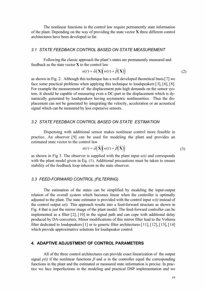
The nonlinear functions in the control law require permanently state information of the plant. Depending on the way of providing the state vector X three different control architectures have been developed so far.
3.1 STATE FEEDBACK CONTROL BASED ON STATE MEASUREMENT Following the classic approach the plant’s states are permanently measured and feedback as the state vector X to the control law
( ) ( )( )u t w t( ) $ ( ) $= +α βX X (2)
as shown in Fig. 2. Although this technique has a well developed theoretical basis [7] we face some practical problems when applying this technique to loudspeakers [3], [6], [8]. For example the measurement of the displacement puts high demands on the sensor sys-tem. It should be capable of measuring even a DC-part in the displacement which is dy-namically generated by loudspeakers having asymmetric nonlinearities. Thus the dis-placement can not be generated by integrating the velocity, acceleration or an acoustical signal which can be measured by less expensive sensors.
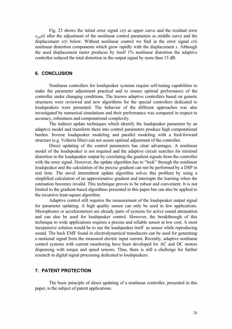
3.2 STATE FEEDBACK CONTROL BASED ON STATE ESTIMATION Dispensing with additional sensor makes nonlinear control more feasible in practice. An observer [9] can be used for modeling the plant and provides an estimated state vector to the control law
( ) ( )( )u t w t( ) $ $ ( ) $ $= +α βX X (3)
as shown in Fig 3. The observer is supplied with the plant input u(t) and corresponds with the plant model given in Eq. (1). Additional precautions must be taken to ensure stability of the feedback loop inherent in the state observer.
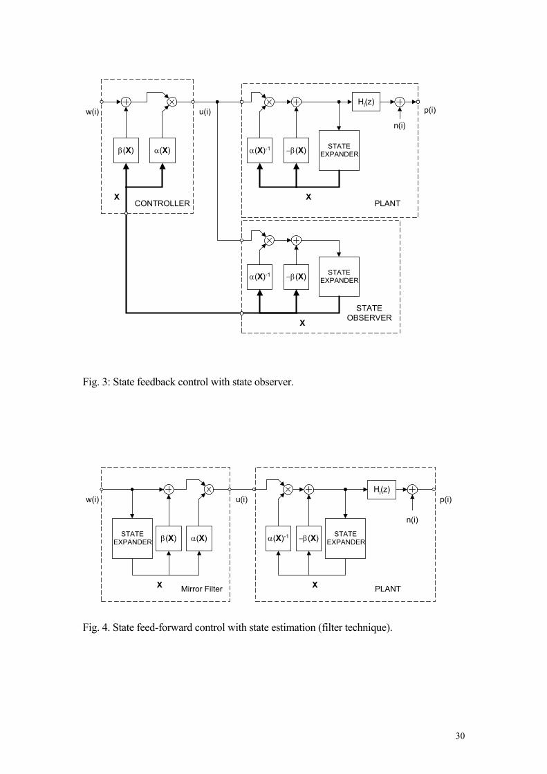
3.3 FEED-FORWARD CONTROL (FILTERING) The estimation of the states can be simplified by modeling the input-output relation of the overall system which becomes linear when the controller is optimally adjusted to the plant. The state estimator is provided with the control input w(t) instead of the control output u(t). This approach results into a feed-forward structure as shown in Fig. 4 that is just the mirror image of the plant model. The feed-forward controller can be implemented as a filter [2], [10] in the signal path and can cope with additional delay produced by DA-converters. Minor modifications of this mirror filter lead to the Volterra filter dedicated to loudspeakers [1] or to generic filter architectures [11], [12], [13], [14] which provide approximative solutions for loudspeaker control.
4. ADAPTIVE ADJUSTMENT OF CONTROL PARAMETERS All of the three control architectures can provide exact linearization of the output signal p(t) if the nonlinear functions β and α in the controller equal the corresponding functions in the plant and the estimated or measured state information is precise. In prac-tice we face imperfections in the modeling and practical DSP implementation and we

20
have to look for an optimal solution which provides the best matching between controller and plant. This optimization problem can be solved by defining a cost function that gives a numerical scaling of the disagreement. Searching for the global minimum of this costs function leads to the optimal parameter setting. In an on-line scenario the cost function also depends on characteristics of the au-dio signal supplied to the loudspeaker. Clearly, the learning of the nonlinear control pa-rameters stagnates when the amplitude of input signal is low and the loudspeaker behaves almost linearly. In the following sections persistent excitation of the plant is assumed. This paper focuses on the adjustment of the nonlinear functions β and α in the nonlinear control law. If the state vector X is not measured at the plant but estimated by the controller the free parameters of the state expander must also be adjusted to the par-ticular plant. However, this issue can be solved by straightforward linear methods [15] and by using the nonlinear parameters identified in the control law. There are two ways for adjusting the controller to the plant. Direct updating of the control parameter has to cope with the nonlinear plant which is part of the update process. Since a stable and robust algorithm for direct updating has not yet been found indirect methods have been used so far [16], [17], [18]. The indirect updating requires an additional adaptive system to model the plant and to transfer identified parameters into the controller afterwards.
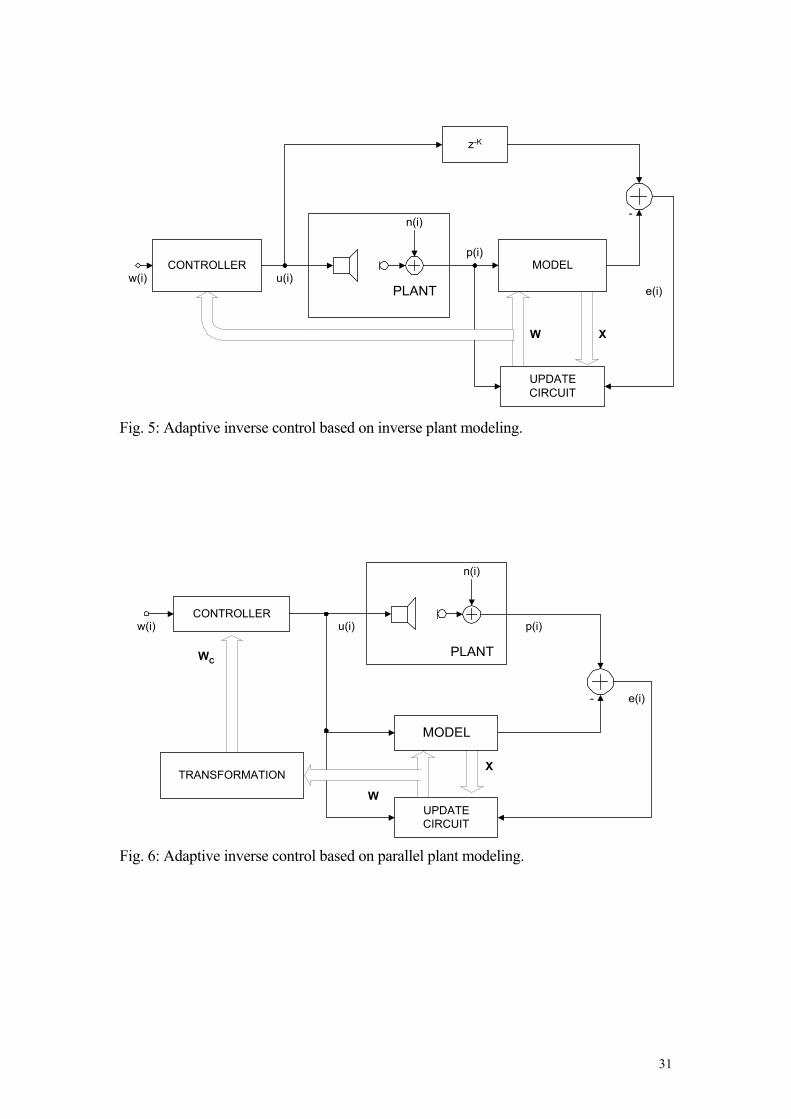
4.1 INDIRECT UPDATING The identification of the plant can be accomplished by an adaptive model con-nected in series or in parallel to the plant. Fig. 5 shows the serial way where the adaptive model compensates for the nonlinearities of the preceding plant by estimating the inverse transfer function. An error signal e(i) is generated by comparing the model output with the delayed plant input u(i-K). The identified parameters W can be copied into the con-troller where they are directly used as control parameters. Contrary, Fig. 6 shows the parallel modeling of the plant where the error signal is defined as the difference between the plant output and the model output. After conver-gence of the parallel model the estimated model parameters W are transformed into con-trol parameters WC and supplied to the controller. Both methods have in common that the error signal is directly calculated from the model output which simplifies the update sys-tem.
4.1.1 Inverse Plant Modeling An adequate structure of the inverse model can be derived from the plant model given by Eq. (1). Fig. 7 shows the corresponding signal flow chart in greater details. The plant output p(i) is supplied via a linear filter to a nonlinear part which is identical with the control law in the controller. The transfer function of the linear filter is just the inverse of the linear system Hl(z) including an additional time delay of K samples to compensate for non-minimal phase properties caused by acoustic propagation. Although the model in Fig. 7 uses a state expander the way of generating the state vector X is irrelevant for the updating of the nonlinear control law. An error signal at the discrete time i is defined by
( )[ ] ( )e i u i K p i K hl( ) ( ) ( ) * $ $ $ $= − − − +−1 β αX X (4)
21
where u(i-K) is the delayed input signal. The control gain and control additive are expanded by
( )( )$
$
α
βα α
β β
X A W
X A W
= +
=
1 T
T (5)
where the vectors Aα and Aβ comprise known functions of state vector X, Wα and Wβ are unknown parameter vectors. This expansion can be realized by using a simple power series or neural networks with adjustable parameters in the output layer or any other expansion being linear in the unknown parameters [19]. Secondarily it is also advantageous for fast convergence of the adaptive scheme that the number of unknown parameters is minimal and the elements of Aα and Aβ are as far as possible statistically independent. After defining the cost function as the mean squared error
( )[ ]MSE J E e i≡ = ( ) 2 (6)
the optimal filter parameters W≡Wopt are determined by searching for the minimum of the cost function where the partial derivatives become
∇ ≡ =ββ
∂∂
( )JJ
optW
0W
(7)
and
∇ ≡ =αα
∂∂
( ) .JJ
optW
0W
(8)
Although this set of simultaneous equations can directly be solved via the Wiener-Hopf equation it is more practical in real time implementation to use an iterative approach. Beginning with an initial values of the parameter vectors Wα(0) and Wβ(0) the next guess of the parameter vector can recursively be determined by the steepest-descent algorithm
[ ] [ ]W W Wα α α ε αµ µ( ) ( ) ( ) ( ) ( ) ( )i i J i E e i e+ = + −∇ = + ∇1 12
(9)
[ ] [ ]W W Wβ β β β βµ µ( ) ( ) ( ) ( ) ( ) ( )i i J i E e i e+ = + −∇ = + ∇1 12
(10)
with the gradient vectors ( )( )∇ = ∗ − +−
α αβ( ) ( ) ( ) $ ( )e p i h i n il1 X A (11)
and ( )∇ =β βα( ) $ ( )e iX A (12)
specified for this particular problem. Omitting the expectation operator in Eqs. (9) and (10) leads to the stochastic gradient-based method
W Wα ε αµ( ) ( ) ( ) ( )i i e i e+ = + ∇1 (13)W Wβ β βµ( ) ( ) ( ) ( )i i e i e+ = + ∇1 (14)
commonly known as LMS-algorithm. Faster convergence speed at the expense of an increase in computational complexity can be obtained by substituting the constant step factor µ in Eqs. (13) and (14) by a variable factor depending on the autocorrelation of the gradient vector leading to the family of least square algorithms. Anyway, the final

22
recursive updating can be accomplished by straightforward algorithms. The interested reader is referred to the wide spectrum of literature relevant to this subject [15]. The particular issue coming up with nonlinear plant modeling is the generation of the gradient vectors which are nonlinear functions of the state vector X and the plant output p(t). The gradient ∇α(e) can easily be generated by tapping the model filter. The calculation of the gradient ∇β(e) requires additional multiplications of the vector Aβ(i) with the instantaneous control gain α(X). Since the controller and the inverse model are based on the same control law the identified parameters of the inverse model can directly be copied into the controller. The inverse modeling ensures stability for any choices of the model parameters since the model is feed-forward regardless whether the states are measured at the plant or generated in the model. Since the cost function is also quadratic in the unknown parameters the adaptation process will not be trapped in local minima. However, inverse system identification has also a major disadvantage: When the measured plant output is corrupted by the noise n(i) as shown in Fig. 7 the estimate of the parameter vector Wβ is biased and leads to a suboptimal solution as shown by Widrow [20].
4.1.2 Parallel Plant Modeling
Parallel modeling as shown in Fig. 6 is an interesting alternative to inverse modeling because the parameter estimation is immune against additional noise at the plant output. The plant model represented by Eq. (1) is of course the best candidate for parallel modeling. Fig. 8 shows the signal flow chart of the plant and the parallel model provided with the measured state vector X. The difference between the real plant output and the estimated output is defined as the error signal
( ) ( )[ ]e i p i p i p i u i h( ) ( ) $( ) ( ) ( ) $ $ *= − = − −−α βX X11 (15)
and the nonlinear functions are expanded by ( ) ( )− + =−u T$ $α βX X A W1 (16)
where W is the unknown parameter vector and A comprises nonlinear functions of the state vector X and voltage u. Contrary to the usual approach in adaptive filtering the cost function is defined here as the mean squared filtered error
( )[ ]MSFE J E e i he≡ = ( ) * 2 (17)
where the Z-transform of he is a causal filter function He(z). The minimum of the cost function
∇ ≡ =( )JJ∂
∂ W0
W
(18)
can be found by using a stochastic gradient-based algorithm ( ) ( )( )[ ]W W( ) ( ) ( ) * *i i e i h e he W e+ = + ∇1 µ (19)
with the simple gradient vector ∇ = ∗W le i h( ) ( )A (20)
In contrast to the algorithm found for inverse modeling the update Eq. (19) requires additional linear filtering of the error signal e(i) and the gradient vector ∇W(e)
23
prior to their multiplication. Whereas H1(z) corresponds with the first-order system of the plant, the filter function He(z) can be chosen arbitrarily. However, there are two configurations of practical interest:
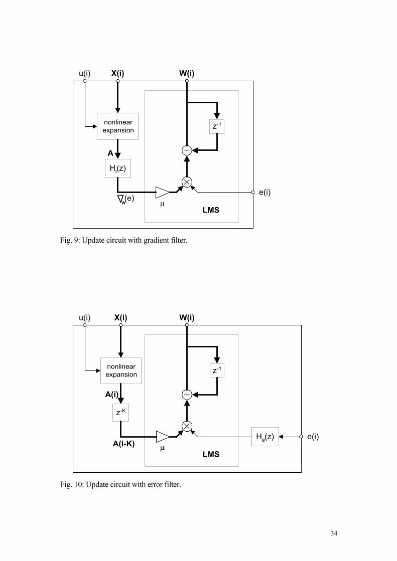
4.1.2.1 Filtered-Gradient Algorithm For He(z)=1 the additional filter in the error path can be omitted and the update equation reduces to
( )[ ]W W A( ) ( ) ( ) * 'i i e i h+ = +1 1µ (21)
related to the diagram presented in Fig. 9. Each element of the gradient vector requires a separate linear filter H1‘(z) which is an estimate of the true response H1(z) in the plant. Whereas an error in the identificaton of the amplitude response is acceptable deviations in the estimated phase response should not exceed ± 90o to keep the update process stable.
4.1.2.2 Filtered-Error Algorithm
The filtered-gradient LMS algorithm is impractical if the dimension of the expansion vector A is high and/or the filter function H1(z) is very complex. In such cases it is advisable to omit additional filtering of the state vector and to use an additional filter He(z) in the error path. If the filter function
H z zH ze
K
( )( )
=−
1
(22)
is just the inverse of the first-order system function H1(z), including an additional time delay of K samples to make He(z) causal, the update algorithm reduces to
( )[ ]W W A( ) ( ) ( ) * ( )i i e i h i Ke+ = + −1 µ . (23)
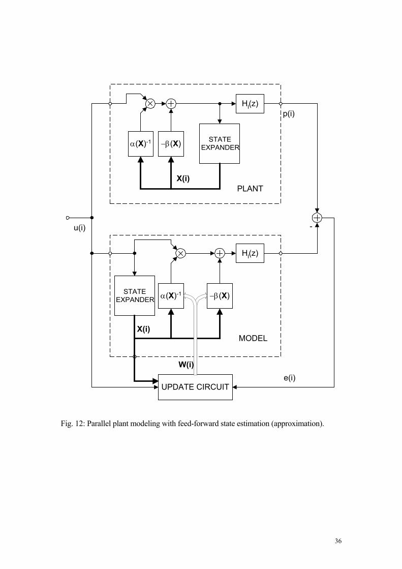
The corresponding diagram of the update circuit is presented in Fig. 10. The additional time delay of the nonlinear state vector and the filter in the error path can easily be implemented in DSP systems. If a permanent measurement of the states at the plant is not practical a state expander is required in the model. According to the structure of the plant the state expander is connected with the nonlinear functions forming a feedback loop as shown in Fig. 11. This model is precise but has the potential for oscillating if the parameter vector W causes a high positive feedback in the loop. Precautions are required in choosing the right starting parameters W(0). This problem can be avoided by using a modified model having a feed-forward structure as shown in Fig. 12. The input u(i) is directly supplied via the state expander to the nonlinear functions. This guarantees stability for all variations of the parameter vector W. Most of the generic nonlinear filters belong to this family. For example the adaptive polynomial filters based on Volterra theory [18] has been used frequently for parallel modeling of loudspeaker systems. The polynomial filters comprise a tapped delay line for producing the state vector X, multipliers and weights for power series expansion of the state vector. These parts can be viewed as the state expander and the nonlinear function β(X) in Fig. 12. Sufficient agreement has been found at small amplitudes when the woofer behaves weakly nonlinear and the effect of the feedback loop can be ignored. However, the feed-forward model fails in explaining the behavior of the woofer at larger

24
amplitudes when the nonlinear distortions of the woofer come in the order of magnitude of the fundamental as shown in prior investigations [22]. The structural disagreement also impairs the accuracy of parameter estimation discussed in the following simulation in greater detail.
4.1.2.3 Simulations in Parallel Plant Modeling The way of generating the state information in parallel plant modeling has a strong influence on the accuracy of the parameter estimation and consequently on the performance of the control system. This effect can systematically be investigated by simulating the adaptive process for a simple example. A woofer mounted in a closed-box has a strong symmetrical nonlinearity in the mechanical suspension represented by the stiffness
k x k k x( ) = +0 22 (24)
where x is the displacement of the voice coil. From the view point of the plant model given in Eq. (1) the quadratic term in the stiffness yields the nonlinear function β(x) = k2x2 which requires the displacement x as state information only. Since all the other elements of the woofer are assumed to be linear the nonlinear function α=1 becomes constant and has not to be considered in the simulation. The state expander is a linear second-order lowpass with a resonance frequency f0 and loss factor Q=2 providing the displacement to the nonlinear function β(x). Using a laser displacement meter as sensor the linear system Hl(s) in the plant is a lowpass which is identical with the state expander. The transfer response of this nonlinear system in respect to the fundamental frequency can be calculated by solving the nonlinear differential equation well known as Duffing’s equation [21]. Fig. 13 shows the frequency response of the displacement as a function of the amplitude U of the sinusoidal input voltage. The bending of the resonance curve to higher frequencies with increasing voltage is a typical effect caused by the progressive stiffness. For a sinusoidal input with U=15V the nonlinear system starts with bifurcation and produces three different solutions (only two of them are stable) causing very interesting jumping effects well known in practice and theory [22], [23], [24], [25]. Applying parallel modeling with state measurement as shown in Fig. 8 to this particular plant we investigate the properties of the cost function defined in Eq. (17) for He(z)=1 in greater detail. For a sinusoidal input with a frequency of f=1.9f0 the mean squared error is depicted in Fig. 14 as a function of estimated parameter k2 normalized to the precise parameter k2 and the amplitude U of the electric input. The mean squared error is zero if the estimated parameter equals the true parameter for all amplitudes U. The error grows smoothly with increasing difference for lower values of the amplitude U. In the region of bifurcation the error surface is not unique but depends on the instantaneous state of the system. However, the filtered-gradient and the filtered-error method represented by Eqs. (21) and (23), respectively, use the exact gradient vector which leads the parameter search downhill on the cost function to the optimal parameter estimate. The cost function of the parallel plant modeling with precise state estimation within the model according to Fig. 11 is presented in Fig. 15. If the amplitude is small the state estimation in the feedback loop generates almost the same cost function as the state measurement. Only for high amplitudes the two nonlinear systems bifurcate separately to different states generating a complicated error surface. Fortunately, the filtered-gradient
25
and the filtered-error method presented here always calculate the exact gradient vector on this surface which also leads to the optimal parameter where the error vanishes for all amplitudes of the electric input. Adaptive parallel modeling with a feed-forward structure such as found in polynomial filters works on a cost function depicted in Fig. 16. This cost function has also a minimum but it turns to higher values of the parameter estimate for increasing amplitude of the input voltage U. Only for low amplitudes of the input signal the estimated parameter corresponds with the true one. The feed-forward structure is not capable to model the bifurcation of the plant at high amplitudes at all and the residual error remains high for any choice of parameter k2. The filtered-gradient and the filtered-error method guarantee a robust and stable convergence to a temporary optimum but the search for the optimal parameters starts again when the amplitude and the spectral properties of the electric signal changes. In summary the parallel modeling of the woofer with a feed-forward structure produces biased estimates on the control parameters which impair the performance of the controller.
4.2 DIRECT UPDATING OF THE CONTROL PARAMETERS Despite the problems already discussed in parallel and inverse plant modeling both techniques require an additional nonlinear system which has almost the same com-plexity as the controller itself. This increases the costs of DSP implementation and might be an obstacle for real time processing. Direct updating of the controller as shown in Fig. 17 is an interesting alternative because it dispenses not only with additional system iden-tification and cumbersome parameter transformation but evaluates the final performance of the controller - the reduction of distortion in the reproduced sound. However, direct updating of the control parameters has been avoided so far because the nonlinearities of the plant have to be considered in the update process. In this paper a novel update algorithm will be presented which copes with this issue. For a controller using permanent measurement of the state vector X at the plant the error signal becomes
( )( ) ( )( ) ( )e i p i p i w i w i hd( ) ( ) ( ) ( ) $ $
( ) *= − = + − −
β
αα
βXXX
X 1 (25)
where the nonlinear function are expanded into ( )$α α αX A W= +1 T
( )$β β βX A W= T . (26)
Like the derivation of the parallel plant modeling the cost function is defined as the mean squared filtered error
( )[ ]MSFE J E e i he≡ = ( ) * 2 (27)
The minimum of the cost function is found by the stochastic gradient-based method
( ) ( )( )[ ]W Wα α αµ( ) ( ) ( ) * *i i e i h e he e+ = + ∇1 (28)
( ) ( )( )[ ]W Wβ β βµ( ) ( ) ( ) * *i i e i h e he e+ = + ∇1 (29)
with the gradient vector
26
( ) ( )( )∇ = ∗ + +
α
ααα
β( ) ( ) ( ) $ ( )e h i w i elA
XX R (30)
and [ ]∇ = ∗ +β β β( ) ( ) ( )e h i el A R (31)
where Rα(e) and Rβ(e) represent further partial derivatives of e(i) in respect to Wα and Wβ. However if the amplitude of the error signal is sufficiently small the right terms Rα(e) and Rβ(e) in Eqs. (30) and (31) vanish and the gradient vectors come close to
( ) ( )( )∇ → ∇ = ∗ +
→ =α α
α
αβ( ) ( ) ( )
$( ) $e e h i w ie e l0 0
AX
X (32)
and ∇ → ∇ = ∗→ =β β β( ) ( ) ( )e e h ie e l0 0
A . (33)
This property gives the idea for developing an intermittent update circuit which dispenses with complicated calculation of the terms Rα(e) and Rβ(e) in a DSP. This system monitors the amplitude of the error and calculates new estimates of the parameter only if the amplitude of the error is below an allowed threshold emax and the simplified gradients∇α(e)|e=0 and∇β(e)|e=0 are good approximations of the true ones.
4.2.1 Intermittent Filtered-Gradient LMS Algorithm For He(z)=1 the additional filter in the error path can be omitted and the update equation reduces to
( ) ( )( )W W AX
Xα ααµ
αβ( ) ( ) ( ) *
$( ) $
( ) max
i i e i h w il
e i e
+ = + ⋅ +
<
1 (34)
( )W W Aβ β βµ( ) ( ) ( )( ) max
i i e i hl e i e+ = + ⋅ ∗
<1 (35)
Fig. 18 shows the corresponding update circuit comprising a nonlinear expansion system, a linear filter H1(z) and an LMS update circuit for each element of the parameter vector. The nonlinear expansion of the state vector and the multiplication with the input signal w(i) can be realized using signals generated in the control law. A switch connected in the error path interrupts the learning when the error e(i) exceeds an allowed threshold.
4.2.2 Intermittent Filtered-Error LMS Algorithm
The complexity of the update circuit can substantially reduced by using an inverse linear filter in the error path prior to the correlation with the gradient. Each element of the gradient vector requires only a delay of K samples to make the error filter with He(z) causal. The update equations
( ) ( ) ( )( )W WA
XXα α
αµα
β δ( ) ( ) ( )$
( ) $ * ( )( ) max
i i h e i w i i Ke
e i e
+ = + ∗ ⋅ +
−
<
1 (36)
( ) ( )W W Aβ β βµ( ) ( ) ( ) ( )( ) max
i i h e i i Ke e i e+ = + ∗ ⋅ −
<1 (37)
correspond with the signal flow chart given in Fig. 19.

27
The update algorithm is not restricted to state feedback control but can also applied to controllers having a separate state expander when using the estimated states X in Eqs. (34) to (37).
4.2.3 Simulations in Direct Control A state feedback controller with direct updating is applied to the woofer defined in section 4.2.3 to investigate the adaptive algorithm in greater detail. Fig. 20 shows the cost function as define in Eq. (27) in dependence of the control parameters k2/k2 and the amplitude U of an excitation tone at 1,9f0. The mean squared error grows with the ampli-tude U and the disagreement between the control parameter k2 and the “true” parameter k2 of the plant. If the nonlinear control is not active (k2<<k2) the state of the plant bifur-cates into different solutions for high amplitudes of U. Improving the adjustment the bi-furcation stops (contrary to the parallel plant modeling) and the woofer behaves more and more like a linear system. Finally, when the controller matches the plant (k2/k2=1) the nonlinearities are completely compensated in the overall system and the error vanishes for all amplitudes U. However, the update circuit needs the gradient vector to find the optimal parame-ters in the minimum of the cost function. Figs. 21 and 22 shows the amplitude and phase, respectively, of the gradient vector ∇β(e) as functions of the control parameter and the amplitude U. These functions represented by both kinds of symbols (cross and circled cross) are almost constant over a wide range but develop a complicated characteristic in the region of bifurcation. If the phase of gradient is not calculated precisely and deviates more than 900 from the true values the update algorithm diverges. Since, the precise cal-culation of the gradient vector can not realized on current DSP-systems the proposed in-termittent learning procedure uses the simplified gradient ∇β(e)|e=0 as a sufficient ap-proximation for the precise gradient in the area of the circled crosses in Figs. 21 and 22. The update process is interrupted when the error exceeds an allowed threshold (emax= -20 dB) and the simplified gradient is likely to fail. The abandoned gradient signals are repre-sented by crosses in the plot. For stochastic signals with persistent excitation (e.g. the most audio signals) the normal fluctuations in amplitude and spectral characteristics ensure that the learning process is not permanently blocked as observed in present simulation using stationary si-nusoidal tones. The number and duration of the interruptions decrease with the progress of the adaptation until the error is small enough that the update circuit can permanently use the simplified gradient for all input signals.
5. PRACTICAL IMPLEMENTATION The mirror filter with direct parameter updating has been implemented in a DSP56002 and has been used for controlling a woofer mounted into a closed-box system. A Laser displacement meter Keyance LB72 provided the adaptive filter with the measured displacement of the cone. Exciting the speaker via the controller with noise or music the control parameters converged to optimal values after a few minutes. The intermittent technique assures robustness of the update process even for loudspeakers with strong nonlinearities.
28
Fig. 23 shows the initial error signal e(t) as upper curve and the residual error eopt(t) after the adjustment of the nonlinear control parameters as middle curve and the displacement x(t) below. Without nonlinear control we find in the error signal e(t) nonlinear distortion components which grow rapidly with the displacement x. Although the used displacement meter produces by itself 1% nonlinear distortion the adaptive controller reduced the total distortion in the output signal by more than 15 dB.
6. CONCLUSION Nonlinear controllers for loudspeaker systems require self-tuning capabilities to make the parameter adjustment practical and to ensure optimal performance of the controller under changing conditions. The known adaptive controllers based on generic structures were reviewed and new algorithms for the special controllers dedicated to loudspeakers were presented. The behavior of the different approaches was also investigated by numerical simulations and their performance was compared in respect to accuracy, robustness and computational complexity. The indirect update techniques which identify the loudspeaker parameter by an adaptive model and transform them into control parameters produce high computational burden. Inverse loudspeaker modeling and parallel modeling with a feed-forward structure (e.g. Volterra filter) can not assure optimal adjustment of the controller. Direct updating of the control parameters has clear advantages. A nonlinear model of the loudspeaker is not required and the adaptive circuit searches for minimal distortion in the loudspeaker output by correlating the gradient signals from the controller with the error signal. However, the update algorithm has to “look” through the nonlinear loudspeaker and the calculation of the precise gradient can not be performed by a DSP in real time. The novel intermittent update algorithm solves this problem by using a simplified calculation of an approximative gradient and interrupts the learning when the estimation becomes invalid. This technique proves to be robust and convenient. It is not limited to the gradient-based algorithms presented in this paper but can also be applied to the recursive least-square algorithm. Adaptive control still requires the measurement of the loudspeaker output signal for parameter updating. A high quality sensor can only be used in few applications. Microphones or accelerometers are already parts of systems for active sound attenuation and can also be used for loudspeaker control. However, the breakthrough of this technique to wide applications requires a precise and reliable sensor at low cost. A most inexpensive solution would be to use the loudspeaker itself as sensor while reproducing sound. The back EMF found in electrodynamical transducers can be used for generating a motional signal from the measured electric input current. Recently, adaptive nonlinear control systems with current monitoring have been developed for AC and DC motors dispensing with torque and speed sensors. Thus, there is still a challenge for further research in digital signal processing dedicated to loudspeakers.
7. PATENT PROTECTION The basic principle of direct updating of a nonlinear controller, presented in this paper, is the subject of patent applications.

29
−β(X)α(X)-1 STATEEXPANDER
X(i)
Hl(z)p(i)u(i)
PLANT
n(i)
LOUDSPEAKER SENSORu(t) p(t)
Fig. 1: Nonlinear model of the plant (loudspeaker + sensor).
α(X) −β(X)α(X)-1β(X) STATEEXPANDER
X
Hl(z)p(i)u(i)w(i)
PLANTCONTROLLER
n(i)
Fig. 2: State feedback control based on state measurement.
30
α(X)β(X)
X
u(i)w(i)
CONTROLLER
−β(X)α(X)-1 STATEEXPANDER
X
STATEOBSERVER
−β(X)α(X)-1 STATEEXPANDER
X
Hl(z)p(i)
PLANT
n(i)
Fig. 3: State feedback control with state observer.
α(X) −β(X)α(X)-1β(X)STATEEXPANDER
STATEEXPANDER
XX
Hl(z)p(i)u(i)w(i)
Mirror Filter PLANT
n(i)
Fig. 4. State feed-forward control with state estimation (filter technique).
31
CONTROLLERp(i)
w(i)
W
-
UPDATECIRCUIT
n(i)
PLANTu(i)
e(i)
z-K
W
MODEL
X
Fig. 5: Adaptive inverse control based on inverse plant modeling.
CONTROLLER
e(i)
p(i)w(i)
WC
-
UPDATECIRCUIT
TRANSFORMATION
MODEL
n(i)
PLANT
u(i)
X
e(i)
W
Fig. 6: Adaptive inverse control based on parallel plant modeling.

32
p(i)
u(i)
α(X)β(X)STATEEXPANDER
XINVERSE MODEL
−β(X)α(X)-1 STATEEXPANDER
X
Hl(z)
PLANT
n(i)
z-K
1Hl(z)zK
UPDATECIRCUIT
e(i)
W
-
Fig. 7: Inverse plant modeling with state estimation.

33
u(i)
−β(X)α(X)-1 STATEEXPANDER
X
Hl(z)p(i)
PLANT
−β(X)α(X)-1
X
MODEL
Hl(z)
W
e(i)
UPDATE CIRCUIT
-state
measurement
p(i)
Fig. 8: Parallel plant modeling with state measurement.
34
nonlinearexpansion z-1
Hl(z)
X(i)u(i) W(i)
e(i)
LMSµW
(e)
A
Fig. 9: Update circuit with gradient filter.
nonlinearexpansion z-1
z-K
He(z)
X(i)u(i) W(i)
e(i)
A(i)
LMSµA(i-K)
Fig. 10: Update circuit with error filter.

35
u(i)
−β(X)α(X)-1 STATEEXPANDER
X
Hl(z)p(i)
PLANT
−β(X)α(X)-1 STATEEXPANDER
X(i)MODEL
Hl(z)
W(i)e(i)
-
UPDATE CIRCUIT
Fig. 11: Parallel plant modeling with precise state estimation (feedback model).
36
u(i)
−β(X)α(X)-1 STATEEXPANDER
X(i)
Hl(z)p(i)
PLANT
−β(X)α(X)-1
X(i)MODEL
Hl(z)
W(i)e(i)
UPDATE CIRCUIT
-
STATEEXPANDER
Fig. 12: Parallel plant modeling with feed-forward state estimation (approximation).

37
Fig. 13: Amplitude response of the displacement of a woofer with nonlinear suspen-sion in dependence on the input voltage.

38
Fig. 14: Mean squared error as a function of parameter ratio and voltage of the sinu-soidal input for parallel plant modeling with state measurement.
Fig. 15: Cost function depending on parameter ratio and voltage of the sinusoidal in-put for parallel plant modeling with feedback state estimation (precise model).

39
Fig. 16: Cost function depending on parameter ratio and voltage of the sinusoidal in-put for parallel modeling based on feed-forward state estimation.


41
CONTROLLERp(i)w(i)
W(i)
-
UPDATECIRCUIT
n(i)
PLANTu(i)
e(i)
Hl(z)
X(i)
pD(i)
Fig. 17: Direct adaptive inverse control.
nonlinearexpansion z-1
Hl(z)
X(i)u(i) W(i)
e(i)
LMSµW
(e)|e|>emax
A(i)
Fig. 18: Intermittent update circuit for direct adaptive control with gradient filter.

42
nonlinearexpansion z-1
X(i)w(i) W(i)
e(i)
LMSµ |e|>emax
He(z)
z-K
Α(ι−Κ)
Fig. 19: Intermittent update circuit for direct adaptive control with error filter.

43
Fig. 20: Cost function depending on parameter ratio and voltage of the sinusoidal input for direct adaptive control.

44
Fig. 21: Amplitude of the gradient signal as a function of parameter ratio and volt-age of the sinusoidal input in direct adaptive control.

45
Fig. 22: Phase of the gradient signal as a function of parameter ratio and voltage of the sinusoidal input in direct adaptive control.

46
Fig. 23: Error signal without (above) and with (middle) nonlinear control and the displacement of the voice coil (below).
8. REFERENCES [1] A.J. Kaiser, “Modeling of the Nonlinear Response of an Electrodynamic Loudspeaker by a Volterra Series Expansion,” J. Audio Eng. Soc. 35 (1987) 6, p. 421. [2] W. Klippel, “The Mirror filter - a New Basis for Reducing Nonlinear Distortion Reduction and Equalizing Response in Woofer Systems,” J. Audio Eng. Soc., Vol. 32, No. 9, pp. 675-691, (1992). [3] J. Suykens, J. Vandewalle and J. van Gindeuren, “Feedback Linearization of Nonlinear Distortion in Electrodynamic Loudspeakers,” J. Audio Eng. Soc., Vol. 43, No. 9, pp. 690-694 (1995). [4] R. A. Greiner and T. M. Sims, “Loudspeaker Distortion Reduction,” J. Audio Eng. Soc., Vol. 32, No. 12, pp. 956 - 963 (1984). [5] J.A. M. Catrysse, “On the Design of Some Feedback Circuits for Loudspeakers,” J. Audio Eng. Soc, Vol. 33, No. 6, pp. 430- 435 (1985).

47
[6] W. Klippel, “Direct Feedback Linearization of Nonlinear Loudspeaker Systems,” pre-sented at the 102nd Convention of the Audio Eng. Soc., Munich, March 22-25, 1997, preprint 4439. [7] H. Nijmeijer and A.J. van der Schaft, Nonlinear Dynamical Control Systems (Springer, New York, 1990). [8] H. Schurer, C.H. Slump and O.E. Herrmann, “Exact Input-Output Linearization of an Electrodynamical Loudspeaker,” presented at the 101th Convention of the Audio Eng. Soc., Los Angeles, November 8 - 11, 1995, preprint 4334. [9] M.A.H. Beerling, C.H. Slump, O.E. Herrman, “Reduction of Nonlinear Distortion in Loudspeakers with Digital Motional Feedback,” presented at the 96th Convention of the Au-dio Eng. Soc., Amsterdam, February 26 - March 1, 1994, preprint 3820. [10] W. Klippel, “Compensation for Nonlinear Distortion of Horn Loudspeakers by Digital Signal Processing,” J. Audio Eng. Soc., vol. 44, pp. 964-972, (1996 Nov.). [11] W. A. Frank, “An Efficient Approximation to the Quadratic Volterra Filter and its Appli-cation in Real-Time Loudspeaker Linearization,” Signal Processing, vol. 45, pp. 97-113, (1995). [12] S. Low and O.J. Hawksford, “A Neural Network Approach to the Adaptive Correction of Loudspeaker Nonlinearities,” presented at the 95th Convention 1993 October 7-10, New York, preprint 3751. [13] P. Chang, C. Lin and B. Yeh, “Inverse Filtering of a Loudspeaker and Room Acoustics us-ing Time-delay Neural Networks,” J. Acoust. Soc. Am. 95 (6), June 1994, pp. 3400 -3408. [14] H. Schurer, C.H. Slump and O.E. Herrmann, “Second-order Volterra Inverses for Com-pensation of Loudspeaker Nonlinearity,” Proccedings of the IEEE ASSP Workshop on appli-cations of signal processing to Audio & Acoustics, New Paltz, October 15-18, 1995, pp. 74-78. [15] S. Haykin, “Adaptive Filter Theory,” Prentice Hall, 1991, Englewood Cliffs, New Jersey. [16] F. X.Y. Gao, “Adaptive Linear and Nonlinear Filters,” PhD Thesis, University of Toronto, 1991. [17] F.Y. Gao, “Adaptive Linearization of a Loudspeaker,” presented at 93rd Convention of the Audio Eng. Soc., October 1 -4, 1992, San Francisco, preprint 3377. [18] V.J. Mathews, “Adaptive Polynomial Filters,” IEEE Signal Processing Magazine, pp. 10 - 26, July (1991).

48
[19] K. Hornik, M. Stinchcombe, and H. White, “ Multilayer Feedforward Networks are Universal Approximators, “ Neural Networks, Vol. 2, pp. 359-366 (1989). [20] B. Widrow, D. Shur, and S. Shaffer, “On Adaptive Inverse Control,” in Proceedings of the 15th Asilomar Conference on Circuits, Systems and Computers, 9-11 Nov. 1981, Pacific Grove, CA (IEEE, New York, 1982), pp. 185-189. [21] H. Chihiro, “Nonlinear Oscillations in Physical Systems (McGraw-Hill, New York, 1964). [22] W. Klippel, “Nonlinear Large-Signal Behavior of Electrodynamic Loudspeakers at Low Frequencies,” J. Audio Eng. Soc., Vol. 40, No. 6, pp. 483-496 (1992). [23] W. Klippel, “Das nichtlineare Übertragungsverhalten elektroakustischer Wandler,” Habi-litationsschrift der Technischen Universität Dresden, March 1994. [24] A. Dobucki, “Nontypical Effects in an Electrodynamic Loudspeaker with a Nonhomoge-neous Magnetic Field in the Air Gap and Nonlinear Suspension,” J. Audio Eng. Soc., Vol. 42, No. 7/8, pp. 565-576, (1994). [25] C.H. Sherman and J.L. Butler, “Perturbation Analysis of Nonlinear Effects in Moving Coil Transducers,” J. Acoust. Soc. Am., Vol. 94, No. 5, pp. 2485-2496.