ADAPTIVE IMPLICIT-EXPLICIT FINITE ELEMENT ALGORITHMS … · computer methods in applied mechanics...

COMPUTER METHODS IN APPLIED MECHANICS AND ENGINEERING 78 (1990) 165-179 NORTH-HOLLAND

ADAPTIVE IMPLICIT-EXPLICIT FINITE ELEMENT ALGORITHMS FOR FLUID MECHANICS PROBLEMS*

T.E. TEZDUYAR and J. LIOU Department of Aerospace Engineering and Mechanics and Minnesota Supercomputer Institute,

University of Minnesota, Minneapolis, MN 55455, U.S.A.

Received 10 November 1988 Revised manuscript received 17 April 1989

The adaptive implicit-explicit (ALE) approach is presented for the finite element solution of various problems in computational fluid mechanics. In the AlE approach the elements are dynamically (adaptively) arranged into differently treated groups. The differences in treatment could be based on considerations such as the cost efficiency, the type of spatial or temporal discretization employed, the choice of field equations, etc. Several numerical tests are performed to demonstrate that with this approach substantial savings in the CPU time and memory can be achieved.

1. Introduction

Large-scale problems in computational fluid mechanics may involve linear equation systems with massive global matrices. Matrices of this size usually arise from the implicit time- integration of spatially discretized time-dependent equations or from a direct solution approach to spatially discretized time-independent equations. For example, the incompressible Navier-Stokes equations in the vorticity-stream function formulation involve a time-dependent convection-diffusion equation for the vorticity and a Poisson equation for the stream function. For most problems of practical interest, especially in three dimensions, handling of large global matrices places a very heavy demand on the computational resources in terms of the CPU time and memory. This demand is too heavy to accommodate even for the largest and fastest computers available today. In this paper we describe, in the context of the vorticity-stream function formulation, alternative solution techniques which substantially reduce the need for the storage and factorization of large global matrices.

The implicit-explicit algorithm proposed by Hughes and Liu [1, 2] (for solid mechanics and heat conduction problems) involves static allocation of the implicit and explicit elements based on the stability limit of the explicit algorithm. In [3] the same static allocation approach was applied to fluid mechanics problems. The adaptive implicit-explicit (AIE) scheme was first presented, in its preliminary stage, in [3]. It is based on dynamic grouping of the elements into the implicit and explicit subsets as dictated by the element level stability and accuracy considerations. For this purpose the algorithm monitors the element level Courant number

*This research was sponsored by NASA-Johnson Space Center under contract NAS-9-17892 and by NSF under grant MSM-8796352.

0045-7825/90/$3.50 (~) 1990, Elsevier Science Publishers B.V. (North-Holland)

166 T.E. Tezduyar, J. Liou~ Adaptive implicit-explicit .finite element algorithms

and some measure of the dimensionless wave number. The element level Courant number is based on the local convection and diffusion transport rates whereas the dimensionless wave number reflects the local smoothness of the 'previous' solution and the spatial discretization. The 'previous' solution can come from the previous time step, nonlinear iteration step, or pseudo-time iteration step, whichever is appropriate. In this approach we can have 'implicit refinement' where it is needed. Elsewhere in the domain, computations are performed explicitly thus resulting in savings in memory and CPU time. The savings can be further increased by performing, as often as desired, an equation renumbering at the implicit zones to obtain optimal bandwidths. Compared to the adaptive schemes based on grid-moving or element-subdividing, the AIE method involves minimal bookkeeping and no geometric constraints.

It is important to note that the dynamic grouping of the AIE scheme does not necessarily have to be with respect to implicit and explicit elements. The letters T and 'E' in 'AIE' could be referring to any two procedures. In fact, there is no reason for the number of possible choices to be limited to two. For a given element, the rationale for favoring one procedure over another one could be based on any factor, such as the cost efficiency, the type of spatial or temporal discretization, the differential equations used for modelling, etc. In this paper, as an example, we implement the AIE scheme also in conjunction with the flux corrected transport (FCT) method [4, 5].

2. Problem statement and the finite element formulation

We consider problems governed by the convection-diffusion equation and the two- dimensional incompressible Navier-Stokes equations. For the Navier-Stokes equations we use the vorticity-stream function formulation; this formulation consists of a time-dependent transport equation for the vorticity co and a Poisson equation relating the stream function qJ to the vorticity. Since the procedures for the spatial and temporal discretizations for the convection-diffusion equation are similar to those for the transport equation of the vorticity- stream function formulation, only the latter will be discussed in this section.

The field equations for the vorticity-stream function formulation of the two-dimensional incompressible Navier-Stokes equations are given as

a"t" + u .Vce--- vV=ce, (2.1)

V2~ - -co , (2.2)

where u is the velocity and v is the kinematic viscosity. The incompressibility condition is automatically satisfied by the following definition of the stream function:

~x 2 = u l , (2.3a)

a¢, c~xl = -u2 . (2.3b)

T.E. Tezduyar, J. Liou, Adaptive implicit-explicit finite element algorithms 167

The flow domain can have several internal boundaries corresponding to possible obstacles (holes) in the flow field. In such cases the unknowns of the problem are: the value of the vorticity at all interior points (to,), the value of the vorticity at all boundary points where both components of the velocity are specified (tooq) (this includes all the external and internal solid boundaries), and the value of the stream function at all interior points and on the internal boundaries (0 , q).

The differential equations given by (2.1) and (2.2), together with the initial condition for the vorticity and the suitable boundary conditions for the vorticity and the stream function, can be translated, via a proper variational formulation [6], into a set of ordinary differential equations. That is

]~/l(d,q)a, "!" C,(d,q)O, = F(d,q , OOq, aGq) ,

v,(O)- (V,)o, gd,q - F n ( v , , VGq ) ,

MVGq = Fro(d, q, v , ) ,

where d,q , o , , a , , OGq and aGq c~¢oGq

at ,respectively.

are the vectors of nodal values of ,/,,q, to,,

(2.4a)

(2.4b) (2.5a) (2.5b)

Bt ' °JGq and

R E M A R K 2.1. Particular attention must be paid to the boundary conditions for the vorticity on the (external and internal) solid surfaces and for the stream function on the internal boundaries. Discussion of these boundary conditions and the derivation of the proper variational formulations can be found in [6].

R E M A R K 2.2. Equation systems (2.4a) and (2.5) are derived from the variational formulations corresponding to (2.1) and (2.2), respectively. The initial condition for (2.1) is represented by (2.4b).

R E M A R K 2.3. The matrices X and M are symmetric and positive-definite. The matrix M is topologically one-dimensional because it is associated with the vector VOq co~cresponding to the (unknown) value of the vorticity on the boundaries. The matrices ,t4 and C are functions of the stream function because in the variational formulation of (2.1) we employ a Petrov-Oalerkin method [7] with weighting functions dependent upon the velocity field.

R E M A R K 2.4. Equations (2.4) and (2.5) are solved by employing a predictor/multicorrector algorithm in conjunction with a block-iteration scheme [6]. In fact the way we have written these equations reflects the way the block-iteration scheme works. In the blocks corresponding to (2.4a), (2.5a) and (2.5b), we update v , , d,q and voq, respectively. To move from time step n to n + 1 we start with the predictions

(v , ) °+ l = ( v , ) . + (1 - a ) A t ( a , ) . , (2.6a)

(a,)°+~ = 0 , (2.6b)

168 T.E. Tezduyar, J. Liou, Adaptive implicit.-explicit finite element algorithms

and perform the following iterations:

block 1"

where

and

-- Rn+ ! ,

- i *" i U n + 1 = M ( ( d , q ) . + t ) + a A t C ( ( d , q ) ~ . + t )

Ri,+l

with updates

-- F((d,q)~n+l, (VGq)~n+,, (aGq)in+l) - (l~l((d,q)~n+t)(a,)~,,+~ + C((d,q)in+l)(V,)in+,),

(2.7a)

(2.7b)

(2.70

K(d,q~i+l J+1 i , .+, = Fu( (v , ) , ,+I , (VGq)n+l ) '

M(VGq~i+I i + 1 - ~ i + 1 , . +, = F m ( ( d . q ) . +,, ~,v. ).+ x ) .

The iterations continue until a predetermined convergence criterion is met.

3. The adaptive implidt-explicit (ALE) scheme

In our block-iterative procedure, at every iteration we need to solve three equation systems: (2.7a), (2.8) and (2.9). The cost involved in (2.9) is not major (see Remark 2.3) and therefore we solve it with a direct method. We are mainly interested in minimizing the CPU time and memory demands of equations (2.7a) and (2.8) which, after dropping all the subscripts and superscripts, can be rewritten as follows:

Y¢ Aa = R , (3.1)

Kd = F . (3.2)

(2.8)

(2.9)

block 3:

block 2:

(v, ~+z = (v,)~.+~ + a At(Aa,)~.+~ (2.7d) / n + l

~,+I , , (2.7e) = (a.), ,+, + (Aa.),,+x a, /n+

Here i is the iteration count, At is the time step and a is a parameter which controls the stability and accuracy of the time integration.


We need to remember that K is symmetric and positive-definite but hi, in general, is not. We propose to employ the AIE scheme for both of these equations.

The AIE scheme in the context of the vorticity transport equation B

Let $' be the set of all elements, e = 1, 2 , . . . , nero. The assembly of the global matrix M in (3.1) can be expressed as follows:

M= ~ M', (3.3) ee~g

where , ~ is the element contribution matrix which is obtained by permuting the element level matrix Jfi~. It should be noted that M" has the same dimension as the global matrix ,~ but only as many nonzero entries as n~e (e.g. 4 x 4 for a two-dimensional quadrilateral element with a scalar unknown).

Let $'~ and $'E be the subsets of $' corresponding to the implicit and explicit elements, respectively, such that

,~ffi ~ U ~e, (3.4a)

= $'~ n $'E. (3.4b)

Consequently, from (3.3) we get

ee~ t ee~R

(3.5)

The AIE scheme is based on modifying M by replacing ~ e (Ve E ~E) with its lumped mass matrix part, that is

eE~ ! e E ~ .

(3.6)

The grouping given by (3.4) is done dynamically (adaptively) based on the stability and accuracy considerations.

The stability criterion is in terms of the element Courant number Ca, which is defined as

cA,- Ilull At/h, (3.7)

where h is the 'element length' [7]. Any element with its Courant number greater than the stability limit of the explicit method should belong to the implicit group $'~.

For accuracy considerations we use a quantity which is meant to be a measure of the dimensionless wave number [7]. For this purpose, in [3] the 'jump' in the solution across an element was defined as

j ' ( ~ ) = (max ( ~ ] ) - main (~e))/((Oma x - - ~min) , (3.8)

170 T.E. Tezduyar, J. Liou, Adaptive implicit-explicit finite element algorithms

where a is the element node number and co~ is the value of the dependent variable co at node a of the element e. The instantaneous global maximum and minimum values of ~o are denoted by COm, , and Wmi n. This definition reflects the magnitude of the variation of the solution across an element. It was proposed in [3] that the elements with jumps greater than a predetermined value should belong to the group ~ .

In our numerical tests involving one-dimensional propagation of various triangular profiles we observed that the accuracy of the solution is affected not only by the jump in the solution but also by the derivative of the flux of the dependent variable. Therefore, as an alternative criterion we propose to employ the product of the jump and the derivatives of the flux; that is

++=r(°)Cl+,°)l a x I

+ 1+2o) 1) a x 2

A global scaling is needed for this quantity and we propose the following one:

where

, + ( 3 . 1 o ) 0"~ ---- O" ]O'ma x ,

e O'ma x = m a x

e e ~ aX t

+ I a(u2c°) I)e (3.11) ax 2

In this case the elements with cr~ greater than a predetermined value belong to group $'~. Implementation of the AIE scheme is quite straightforward. A global search is performed

on the entire set of elements. With this search, based on the two criteria given by (3.7) and (3.10), the elements are grouped into the subsets ~'~ and ~ .

REMARK 3.1. In the AIE approach one can have a high degree of refinement throughout the mesh and raise the implicit flag only for those elements which need to be treated implicitly.

REMARK 3.2. The savings in the CPU time and memory can be maximized by performing, as often as desired, an equation renumbering at the 'implicit zones' to obtain optimal bandwidths. Bandwidth optimizers are already available for finite element applications, especially in the area of structural mechanics.

REMARK 3.3. Time-dependent convection-diffusion of a passive scalar can be treated as a

special case of (2.1) with the velocity field u given. The only equation system that needs to be solved is (3.1).

The AIE scheme in the context of the flux.corrected transport (FCT) method

The AIE scheme does not have to be based only on implicit-explicit grouping. It can be based on any element level, dynamic, and rational selection between an 'I-procedure' and an 'E-procedure'. Here we give an example by employing the AIE scheme in conjunction with the FCT method described in [4, 5]. We apply this method to the time-dependent convection- diffusion of a passive scalar (see Remark 3.3).


The FCT method given in [4,5] is based on correction of the flux obtained with a lower-order scheme with the flux obtained with a higher-order scheme, while limiting the maximum allowable correction. The balance law is satisfied at the element level. In our case, as the lower-order scheme we use the one-pass explicit SUPG method and as the higher-order scheme the multi-pass explicit SUPG method. With a sufficient number of iterations (typically three) the multi-pass explicit method produces solutions indistinguishable from those obtained by the implicit method. In the utilization of our AIE scheme we define the 'E-procedure' to be the one-pass explicit SUPG method alone and the 'I-procedure' to be the FCT method based on the lower- and higher-order schemes described above.

R E M A R K 3 .4 . Variations of the Taylor-Galerkin method have been used in [5] as lower- and higher-order discretization techniques. We consider the Taylor-Galerkin method to be a close kin (under some circumstances a special case) of the SUPG method proposed in [8-!0]. One can easily see the close connection between the Taylor-Galerkin method and the one-pass explicit 'temporal criterion'-based 'A2-form ' of the SUPG method described in [8-10]. It is not our intention here to make any statement about what lower- and higher-order schemes should be used with the FCT method or about whether the FCT method should be preferred over some other method. We just want to give an example.

For the AIE scheme we employ the explicit 'v-form' of the predictor/muiticorrector algorithm described by (2.7). That is

ML(&v*)',,+I - R',,+t, (3.12a)

where M L is the (diagonal) lumped mass matrix version of .~ and

- A t e , ÷ ° " ÷, +1 - M ( ( v , ) ' . - (v , ) . ) - A t C ' ( a ( v , ) ' . + 1 + (1 - a ) ( v , ) . ) . (3.12b)

Note that these expressions are quite simple due to the fact that this is a linear problem and that no stream function is involved. - i

The nodal value correction vector (&v,)i,+l and the residual vector R.+t can be written as sums of their element level contribution vectors:

Y. (AV: ' ) n + l , eE~g

+1 eEg

(3.13)

(3.14)

The AIE/FCT scheme employed is outlined below:

1. Given (v , ) , , calculate a predicted value for (v,).+l"

(v,)°.. ÷ _ (v,). + (I - At(a, ). I (3.15)

2. Based on this predicted value, by using a lower-order scheme calculate a lower-order residual t~e~°w VeE ~'; compute the lower-order correction corresponding to this V'" ] n + l

172 T.E. Tezduyar, J. Liou, Adaptive implicit-explicit Jinite element algorithms

residual and determine the lower-order solution:

(Av~l°w =ML 1 ~low VeE ,.+1 (R',,.+, , (3.16)

.,o~ o + y. (Av:~,ow V*)n+1-'(V*)n+l In+l" eE~

(3.17)

3. Based on the predicted value (v,)°+l calculate the residual - e 0 (R) .+ 1 Ve E ~ and compute the correction corresponding to this residual:

(AV,)n+,e o = MLX(~.)0+x V e E ~i. (3 .18)

4. Shift the correction (Avg)°+! Ve~ ~i by subtracting the lower-order corrections and determine the first iterative solution:

i~ -0 ,

(AAv~ o ( ( A v : o ~ , o ~ )n+1 ~-~ (ce)O+1 )n+1 - ( A v , ) . + I ) Ve e ~I (3.19)

_- ~ow 0 (3.20) (v,)'.+, (v,,.÷, + Y~ (AAv:).÷x. e ~ I

Here , i (c)n+l is a parameter [4, 5] determined by the maximum correction allowed for element e.

5. Perform a desired number of iterations (nvcv); in each iteration, compute the higher- order correction and determine the FCT solution (based on the higher-order correction and the lower-order solution):

i * " i + l ,

(Av~ I -1 -~ i ).+1 Ve , =M~ (S) .+ , ~Z , (3.21)

(AAv: ' ((AAv: ~-~ ).÷~=(c')'.÷, ).÷, +(a~: ) .÷ , ) V e ~ , , (3.22)

~,i+1 ,~low i V,)n+~ ffi (v, + ~ (AAv.~ (3.23) n + I I n + l

if i < nFc r then goto 5.

6. Pick up the value of the last iterative solution:

( V '~i+1 (v*).+1 ~ *J.+1

and goto the next time step:

(3.24)

n ~ n + l

goto 1.

Limiting the steps 3-6 to the group ~ results in savings in the computational cost involved.


Solution o f the discrete Poisson equation

We use a preconditioned conjugate gradient method [11] to solve the equation system given by (3.2). In conjunction with the AIE scheme employed for (3.1) we define our pre- conditioner matrix P to be

P = ~ K*+ ~ diag(K*), (3.25)

where K e is the element contribution matrix of K. If ~F = ~ then P = g and the solution technique becomes a direct one. If ~[ = g then the method becomes a Jacobi iteration [11]. Other definitions for P are of course possible; the one given by (3.25) is quite simple to implement.

R E M A R K 3.5. The incompressible Navier-Stokes equations in the velocity-pressure formulation, upon spatial and temporal discretizations, can also translate to a set of equations given by (3.1) and (3.2). In this case (3.1) and (3.2) would correspond, respectively, to the momentum equation and the incompressibility constraint. The latter would consist of a discrete Poisson equation for pressure.

R E M A R K 3.6. Another example for the type of problems which can translate to (3.1) and (3.2) is the electrophoresis separation process (see [12]). In the context of a block-iteration scheme, the time-dependent transport equation for the chemical species and the equation for the electric potential would transform to (3.1) and (3.2), respectively.

4. Numerical tests

We have tested the AIE algorithm on problems governed by the convection-diffusion and the two-dimensional incompressible Navier-Stokes equations.

One-dimensional pure advection o f a cosine wave

The purpose of this simple test is to pro;~de a conceptual illustration of the way the AIE scheme works. A cosine wave of unit amplitude is being advected from the left to the right with an advection velocity of 1.0. A uniform mesh is being used and the element Courant number is 0.8.

The AIE scheme is based on selection between the implicit and the one-pass explicit versions of the streamline-upwind/Petrov-Galerkin (SUPG) procedure. The threshold value for the test parameter given by (3.10) is 10 -s. Figure 1 shows the solution and the corresponding distribution of the implicit elements at time steps 0, 50 and 100. Compared to the implicit method, the AIE scheme results in a reduction of 80% in the CPU time and 81% in the memory needed for the global matrix; the solutions obtained by the implicit and the AIE schemes are indistinguishable.


/ l l IlHIll1111111111111111111[llllllllllltlllll, I ~ t ~ i ~ i ~ t ~ i ~ t ~ t i ~ q ~ i ~ i ~ u ~ 1 ~ 1 ~ t ~ 1 1 ~ i ~

~llill~llll~Hll~lli~ll~HlllllilHilllllll~llfllllil~llilllll~ll~lllltilll~i~_ln~lllllllllllltli~li~ill~lllll~llltlllililll~llillllllllh~Lllllllll1ll~lll~lliHl l•lllllL•[llllil1llllllll1llL•illlllllllhl•l•lllilllllllllllll••llllllllllll•l•ll•l•t•tlll••••ll•llllllllilllllllllllllillillllllllHllll•illll•lllllll•lll•lllllill•q•[ulll•ll•l•l•lillq• j

Fig. 1. One-dimensional pure advection of a cosine wave: solution obtained by the AIE SUPG scheme and the corresponding distribution of the implicit elements at t - 0.0, 0.2, 0.4.

•••i•••••i••i••••••T•••i•••••••••••••1••••••••••••i•••••••••••1••••••••1••••1••u••••••••••t••••ji••••••••••••••••••••••••i•••••i•••••• tltllllllllllllllllllllllllllllllllllllnl~llllll

Fig. 2. One-dimensional pure advection of a discontinuity: solution obtained by the AIE/FCT scheme and the corresponding distribution of the FCT elements at t = 0.0, 0.2, 0.4.

One-dimensional pure advection of a discontinuity

The conditions in this case are nearly identical to those in the previous case. This time the profile which is being advected is a discontinuity which initially spans four elements. The AIE scheme is based on selection between the one-pass explicit SUPG method and the SUPG/FCT method implemented as described in Section 3. The threshold value for the parameter given by (3.10) is 10 -7. Figure 2 shows the solution and the corresponding distribution of the FCT elements, at time steps 0, 50 and 100. Compared to the full FCT approach the savings in the CPU time is 45%.

Two-dimensional pure advection of a plateau

This test case is for evaluating the performance of the AIE approach for two-dimensional problems with moving sharp fronts. A 40 x 40 mesh is chosen in a 1.0 x 1.0 computational domain. All boundary conditions are Dirichlet type. The advection velocity is in the diagonal direction and has unit magnitude. The time step is 0.01.

The first AIE scheme is based on selection between the explicit and discontinuity-capturing [13]/implicit versions of the SUPG procedure. The threshold value for the parameter given by (3.10) is 10 -4. Figure 3 shows the solution and the distribution of the discontinuity-capturing/ implicit elements at time steps 0, 16 and 32. Compared to the implicit method, the AIE scheme results in a reduction of 45% in the CPU time and 69% in the memory needed for the global matrix.

The second AIE scheme is based on selection between the one-pass explicit and FCT


i • • u m • w w . • . m w • m w l m m m ~ • w s m s m m m m m m m m m m m • m m i w m w m l w m m m m m m m l m w m m m m m m m m m . m . m . m m • m • . m m • ~ i m i m m . m i m m i i m W i l l i m m m w m w m m m w m m m m m l m m m m w , • m m m m • m m l m m m m . m m . • . m • • • • • . m . m • m . l • . m • • m n i m n a m l m m m m m n m m m m o m e l m | m m | m m m m m u m e m l m i • • , i i m m i m m p m u • i i i m i m m i i • • m i m m m a i i i m • • m • i • • I m m m m m i m m m m m m m m m m m m a | m m m m m m m n m m m m n m m m n m i i • • m m m i m m m m m m m m • m m m m m m • m m • m i e • m • i n m m m • i u n m m e l m n m m m m n m m n m m m e m m m m m m m m m m n i m m u m e m e m i i m • m • m i u m m m m m i m m m n m m n m • m i • • m n • i m m i • • • i m i i • • m m m • m m m m • m i m m l m • m m m m m i • • • • m m m m m u i i • e m ~ i • l m i n w m i n i i • n i m n n i i i m i n e i u i s m m i i • n l i i i n • m m m m • m • m • m l m m i m w • m u m m m m n i • m i • i • • i m i m i • I m m m • m m m i m m m m n • i m m m m i • m m • • i i m i l l i • a m • • • • i n m m m m • m m m m m i m m • m m m m m m • m m m m • m i m m l • • • i • • i i m m m n • m m a m m n m m n m m • i m m m i m n m m m m | m | i n • • m m m m i • • • m m n w m m m m m m m m m l i m i • • i m l m • m m m • i m m m i • • n l i • m m m m m m m m m m m i • m • l n • m m m m m i • m m m i i m i m i m m m

e m n m m m m m m n m n m m m m n m m m • m l m m i • m m m m • • m i u

N m B B U W B B B B • B B B • • • • • i i • • • i • • • s i • i i i i m l n r i i i • i W i l l i m i m i e l i m m • • • • m a i l i e i • m m o m m i n m i m i m m m m • • a m • • m m i m m l i • u • m m | m m m i u l m • u u i • i m m m m m m n i m m n m n • m u m n i • • m i w l m i n a e l a m m | n m m m i • n • ~ m • m m m m i m m i m i i m m l • m l m i • m l i i i i | n m m m n m | m n m n n m i n n m a | m n m n n n m m n m i m n e m n g l i n a m n i m m • m m m i m m m m m m i m m i m m m m i m • m m m i m m n • m n i m u m m i m i n n m n m m • m m m m g • i m m m m i u n m m n m m m e m n i l l i l i • • ~ i i l m i i • i l i i i • i n n i i m i i p i i w i i n n m m m n m n m m m w m m m m m m m m m m m m a m m m m m m m m | m m m m n

n m m l m l m m m m m m w • l m l m • w : n m m . w • m • l . • . . • . . | n • m m m l u m • m m = m m m m . m m l m m m m m m l l m m m m m l • • • | l i m m i m | m m m m m m n m m m m m m • n m m m m m m m m m • m m • n l i

n ~ i n m m i m m m n • i n n u i m m l l m m m • i i m i m m u a n o m a n n m m a n a m m n e i n m m a n m n n n i m m m m n n m g m m m • m m m m n n i m i m m | m m m n m m m m m m m m m • n i i m a n n m • i m u i J m | n n n m m m m m m n m m m m • • n m m e m • • • • • i n m e m n n a e m m m n n m m m m m i m • m i m m m m m m m m a m m i a e m l n n m m n • m w m m l

i m m w m m l m . . m m • e

~i~:' . ............ : 11:" . 1 . . . . . . . . . . . . . . . . . : , . • • . . . . . . • • . • . . . . . - • •

' l . l l l l : : : : : : : : : : : : : : : : . . . . . . . . . . : :

. . . . . . . . . . . . . . . . . . . . . . . . . . . .

: : : : : : : : : : : : : : : : : : : : : : : : : : : : : - .1

: : : : : : : : : : : : : : : : : : : : : : : : : : .1:111:1 , . . . . . , . . . . . . . . . . . . . . . . . . • • • . m • . . . . . . . . . . • • . • . . . . . . . . • . . . . . . ° . . . , . . . . . . . . . . . . . . . . . . . . , m . w . . i • m . • |

i w • • m m m m m • H m n w • l • m • • . • • • • . • • m • | • • = . o • . • . . . . . • |

Fig. 3. Two-dimensional pure advection of a plateau: solution obtained by the AIE SUPGIdiscontinuity-capturing scheme and the corresponding distribution of the discontinuity-capturing/implicit elements at t = 0.0, 0.24, 0.48.

versions of the SUPG procedure. The threshold value for the paramete~ given by (3.10) is 10 -4. Figure 4 shows the solution and the distribution of the FCT elements at time steps 0, 16 and 32. Compared to full FCT approach the AIE scheme results in a 35% reduction in CPU time.

Flow past a circular cylinder at Reynolds number 100

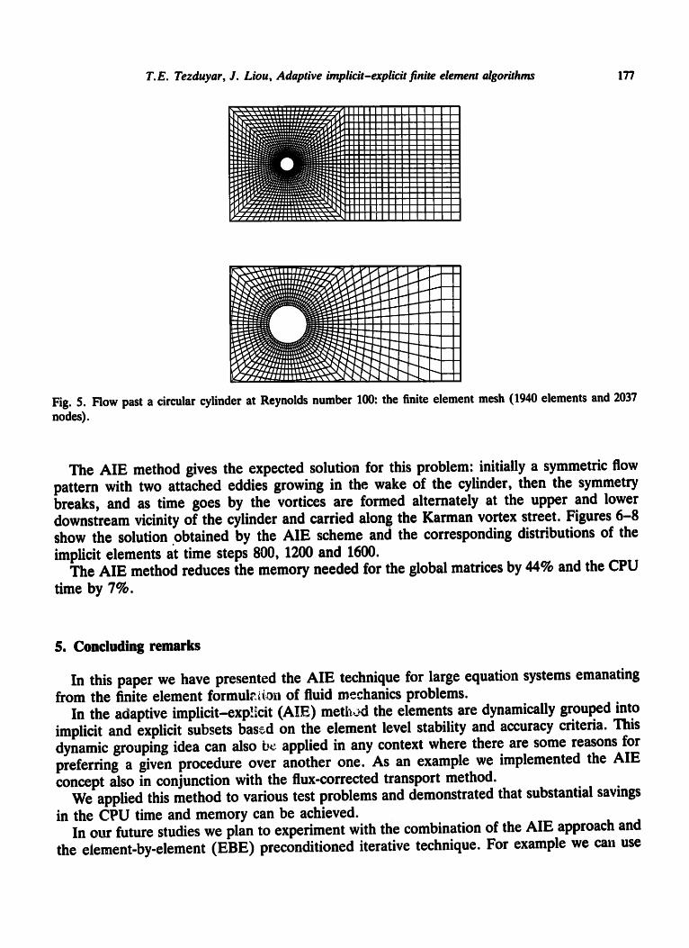
In this problem we use a mesh (see Fig. 5) with 1940 elements and 2037 nodal points. The dimensions of the computational domain, normalized by the cylinder diameter, are 16 and 8 in the flow and the cross flow directions, respectively. The free-stream velocity is 0.125 and the initial value of the vorticity is zero everywhere in the domain. The time step is 1.0.

176 T.E. Tezduyar, J. Liou, Adaptive implicit-e~'plicit finite element algorithms

I I I I I I l l l l l l l l I I I I I I I I I I I I l l l l l l l l l l l l l I l l l l I I I I I I I m l l l l l l l l l l I I I I I I I n l l l l l l l l I I I IN I I I I I I I I I I I I I I I I I I I I I I I I I I I I I I I I I I I I I l l I I I I I I I I I I I I I I I I I I I I I I I I I I I I I I I I I I I I I I I I I I I I I I I I I m l l • I I N I I I I m i l l I I I I I I I I I I I I I ilmni iN nlmmlm nmmlmml miNI mnmmmmmmmmmmmmmmmml

lmml~mmmmm_.llmm mmmmmmmm mmmm)mm~m_mm_mml mm_mmmmmmmmmmmmmmmmmmmmm-ml mmmmI

ii mm mlm mmm mmmmmm mm~mmmm mmmmlmmmmmm mmmmmmmmmmmlmm mmmm mmmmlm imm mm mmmmmmm mmm mm iN mmmmmlmm~mmmm mmmmml immmmmmm mmmlmmmmmmmlmlmmmmmmlmlm im mmm mmlm mmmmmm mmm ma ii m m im m mm m im m mm mmm m m Im mm m mm mm m m i m mm m I mm mm mmlm m mm m m m m m m m ~mmmm mmml imm mm nmlmllmmmmmmmm mm mmmmllm mmmmmmmm immmmmmmmm mmm mmm mmmmmmm mmmm m mmmmmmmmmmmmmmmmmmml ii mmmlm mini mmmm mm mmmmm mmm mmlm mmlmmmm mmmmm mmm mmmm mmmmm ~mm m mmmm mmm m m mm m m mmLm mm mm m m m mmm m mmmmmmmmmmmmmmmmmmm

Mm im mmmmm mmmmmmmmmlmmm immmmlmmmmmmmmmmmmml

im mlm mmmmll m mm mml mllm m m m m m mlm mmmmmmmImmmmm immmmml

i ummmmmmmmmmmmmmmmmm I 11111111111111111111 i i i i i i i i i i i i i i i i i i i i i i i i l l l l l l l l l l l l l i i i i i l l l l l l l l m l l l l i i i i i i i i i l l l l l l l l l l l i l m l l l l l l l l m m N i l l l i i i i i i i i i i l l l l l l l l l l i i i i i i i l l l m l l l l l l l I i i l l l l l l l l l l l l l l l l l i i i i i i i i i i i i i i i i i i i i m l l l l l m l l l l l l l m l l l m i lm l l l l I l = l l l lN I Im l l

I I I I I I I I I l l i l l m i l l ~ l n lmnmmmmml l l lmmml l m HNI I I I I I I I I I IN I I I I I i l l i i i i i i l un i i i i i i i i I I I I

I I I I m l l l l l l l l l l l l l l l I I I I I I I I I I I I I N I I I I i l m l l l m l l l l l l l l l l l l N I I I N I I I N I I I N I N I I I I i i i i i i i I i mN Im l l l I I I I I i i i i I I I I i m l l l l l l l l l I I I I I I I I I I I I I I I I I I I I I I I I I I I I l l l IN I I I I i i i i i i i i i i i i i i i i i i i i I I I IN I I I l l l I I I I I lm l l I I I I m i l l I I I I I I I m l lR I I Im NN I I I IN I I I I I I I I IN I I I I i i i i i i i i i i i i i i i i i i i I I I I I I I I I I I I I I I I I I I I I I l l l l l l l l l l l l l l l N I I I I N I N I N I I I I I I N N I I I I I I I I N m l l l l l l l l l l l l l I I I I N N I I I I I I I I ~ I I I I

n | | |mmm| | | | |m | | | |m |mmmmm| | |m |mmmnm|m|mml immmmmmmmmmmmmmmmammmmmmmmmmmmmmmammmmma immmmmmmlmmmmmmmmmmmmmmmmmmmmmmmmmmmmmml immmmmmmmmmmmmmmmmmmmmmmmmmummmmmmmnmmmn i lmmmmmmmammmmmamlmmmlm lum lmAmlwmmmmmmml L N I I I I I I I I I I I I I I I I I I I N I I I I N I I I I I I I N I I I I

iiiii! iii!ii iii!iiii!!ii :iii Q{iil Lmmm ~mmmmmmmn Immm mmmmmmmmu mum mmmmmmmmmn Im mmmmmmmmmn

immmmmmmmmmmmmmmm~mmi ImmmmNmmml mmmmmmmmlmmmlmmmmmmmmm~ mmmmmmmmmu

mmmmmmmmmmmmmmmmmmmNmmu mmlmmlmmma nmmlmmmmmlm lmmmmmmlwmmmmw mmNmmlmmmn I I I I I I N I I I I I I I I I I I I I I R I I I IN I IN I IN I I i i I N N I N I i I m l n I I I I I N I I I I I I I I I N N I I I I I I I I I I I l l l l l l l l l l l l l l l I m N I INUNI I IN I I i I I I I I I R I I I I I I m l l l l l l R N I I I I I I m l l l l l I N I I I N I R I I I I I I N I I I I I I N l l l I I I I I I I I I I I N I I I I I m N I I I l I I I I I N I m l l l l H I I lm l l lm l I I I l m I I I l l l m l l m m R I I I I R I I I I l U l l l l l l l I I I I I I I I I I N I I I N I I I I I I R I I I I I I N I I I I I I n m l l n l l l l l l l l N i m l l l n l l l m l NNNIN INNI I I I I I I I N R I I I I I I I I I I N I I I I N I I I I I I I I I I I i l n n l n N N i n l l l l . l l l l l l l l l l l l l l l l l l l l I I I I l l l m m l l n l l l l n l l l l h U l l I I I N I I I I I I | N I I N N I I I B N I N I I I I N I N I m l l mN I I l l lm l l I m l l l m l l l l l m l l l l l l l l l l l l I I I I m N I I I I I l l l l l l l l l l l l l . l l l l l l m l I I I I I I I I I I I I I I I I I I m l m l m l l l m l l l l l l I I I I I N g l l l l l l I I I I N N I I N I N I I I I I I I N I N I l I I I I I I I I I I I I l l l lmmNml l lm lm l i i im l I I I I I I m l l l l l m N I I I I I I I N I I I I m l I I I m m l l I I I I I I I I I I I I N I I I

Fig. 4. Two-dimensional pure advection of a plateau: solution obtained by the AIE SUPGIFCT scheme and the corresponding distribution of the FCT elements at t - 0.0, 0.24, 0.48.

The AIE scheme employed .to solve the vorticity transport equation and the Poisson equation is exactly as described in Section 3. For the vorticity transport equation, both the implicit and the explicit methods are SUPG based and involve three iterations per time step. In this problem we estimate the maximum element Courant number to be somewhere around 1.5-1.6; therefore the stability criterion given by (3.7) also becomes active in the implicit- explicit grouping. In fact our numerical experiments show that the computations de not converge when the entire set of elements belong to the explicit group. The threshold value of the parameter given by (3.10) is 10 -5. For the solution of the discrete Poisson equation, the iterations continue until the residual norm falls below 10 -6 or its ratio to the initial residual norm reaches 10 -4 .


lm, l s s m im mm me mw~ar

lUUU ue. :~'." : ::~.~ ~ ' : : ' . ' - ' . .mn l l m g e m - - ; ' . ' - : - ~ - O ~ - ' : l : ' ' 'mummmNil

m -

Fig. 5. Flow past a circular cylinder at Reynolds number 100: the finite element mesh (1940 elements and 2037 nodes).

The AIE method gives the expected solution for this problem: initially a symmetric flow pattern with two attached eddies growing in the wake of the cylinder, then the symmetry breaks, and as time goes by the vortices are formed alternately at the upper and lower downstream vicinity of the cylinder and carried along the Karman vortex street. Figures 6-8 show the solution obtained by the AIE scheme and the corresponding distributions of the implicit elements at time steps 800, 1200 and 1600.

The AIE method reduces the memory needed for the global matrices by 44% and the CPU time by 7%.

S. Concluding remarks

In this paper we have presented the AlE technique for large equation systems emanating from the finite element formul~ion of fluid mechanics problems.

In the adaptive implicit-exp!icit (AIE) met|~od the elements are dynamically grouped into implicit and explicit subsets based on the element level stability and accuracy criteria. This dynamic grouping idea can also b~ applied in any context where there are some reasons for preferring a given procedure over another one. As an example we implemented the AIE concept also in conjunction with the flux-corrected transport method.

We applied this method to various test problems and demonstrated that substantial savings in the CPU time and memory can be achieved.

In our future studies we plan to experiment with the combination of the AIE approach and the element-by-element (EBE) preconditioned iterative technique. For example we can use


~..-_.-,-.-.-.-'.':.:::--:.-_~.~pmilmum m, ••• •••••• ~ ~)-'-'_" - - - -.-.::: - -:; .... ~-w~wmmmmmmmmmmimmimmm ~ ( ~-.-';-.'-_'~ ......... ;y;.'-:w~o m m mm mm mmm mi m m i mmmimm

' k~ ~ q q - ~ . ' . ' : . t " " : : "" "." ".'.;~.~'~ ~ ~o cp mmlnm minim mm mm mmmmmiUini Ivm~.k~--.'.'."," : ,','-t't--,~,.%~¢mmmmmmmmmmmimiummmmm [ t I [ • ~ ) ; .'~..:.-6F:::." ':: i:.::.}~t, -. ; • • S, ~' • . . . . . . . . . . mmmmmm~imm~mm~

• :::::::::-'"'T I [ ) ' )~ ; ) ' ;~ ' . ' i ; ; ' -L " ; : ' : - ' ' . . ' 4 ra t w m w s s l l i i i l m m m i m m i ~ # ~ ~ ~-.,t'.-.,/~z:~t-.,;;;.--~( ~ ~ ~ 4 ~ l n i n i l l I l i l i I m i l i I~ p) ~ w'-.?.'y.";::i-t'.-'.'.'~.-q ~ ~ ~ q u q i m |n i m aN i m U m mi m m i m l-~ooj~--- ......... ".-"--'~ ~ ~(~ n n mm m m m m m m m i m mm mm mm I'@ - . . . . : ; ' . ' : : : : . . . . . . . q~.qimiimmimim m m m m i m m i m i lp . , m , ~ m . o . . . . . . . . . . . . . ~ ' , ~ : ~q ~ " ~ ' ~ ' ~ ' ~ ; - : • : --~.~'~'.,,~,~-?~ll i I m m m m i mm m m m m m m m m m

i . . . . . . . . . ". -." ::..-_.'_."_:_.-___%1". ~ I n i m i u u II n u u i m u m m n i q e - . . . . .~;.:.: . . . . . . . - ,p .p l i iNN l min im mini u l m m n It ] t~.'.--'-'..'-, • •;: •: ..'..'.'..'_~-'-=.~la ~ p ,, u m nu m m m m m mm mm m n s m m •

[ ~ { ~ ~ ~ - ~ . ~ ! : : : , ' i . ' ~ ~ ~ j ~ ~ I i I i I in i S l i S i naB imn me i q ~n q t k ~ ~",.- ".',', " . . . . . . . . . . . ".;;;-e ~ ~ w- ~ - i i l i l i n i i R i i l m ~ , l , , . . . . . . . . . . . . . , , # al i i ~ l u . [ . . . ; . : : ". . . . . . i i N N

iiiiiii!i o • . - = :

k j¢~o)~.)'.t..,;.,;;;:t . . . . . . ~.~ ~,,volt limllmiii mml I) @ ~ (~'--.;'.':.':-':-':'.:"-:-~ ~) ~ ~ ~Imm i m m m m i m n m mimmm i:~ ~ ';~:':':';;-':::':-"-'-'-* ~ ~ z ~ m m m m m m m m mm m mm m m mm mm mm m

I~I~-:-:4-~::::::~-~-~111111111111111111

¢

Fig. 6. Flow past a circular cylinder at Reynolds number 100: solution obtained by the AIE SUPG scheme at t--800; from top to bottom: distribution of the implicit elements, vorticity, streamlines and relative streamlines.

Fig. 7. Flow past a circular cylinder at Reynolds number 100: solution obtained by the AIE SUPG scheme at t-1200; from top to bottom: distribution of the implicit elements, vorticity, streamlines, and relative streamlines.

Fig. 8. Flow past a circular cylinder at Reynolds number 100: solution obtained by the AIE SUPG scheme at t--1500; from top to bottom: distribution of the implicit elements, vorticity, streamlines and relative streamlines.

the EBE scheme to solve the discrete Poisson equation for the stream function, employ the AIE scheme to solve the time-dependent transport equation for the vorticity, but use, again, the EBE scheme at the implicit zones of the implicit-explicit distribution.

References

[1] T.J.R. Hughes and W.K. Liu, Implicit-explicit finite elements in transient analysis: Stability theory, J. Appl. Mech. 45 (1978) 371-374.

[2] T.J.R. Hughes and W.K. Liu, Implicit-explicit finite elements in transient analysis: Implementation and numerical examples, J. Appi. Mech. 45 (1978) 375-278.


[lO1

[11] [121

[131

[3] T.E. Tezduyar and J. Liou, Element-by-element and implicit-explicit finite element formulations for computational fluid dynamics, in: R. Olowinski, G.H. Oolub, G.A. Meurant and J. Periaux, eds., First Internat. Symp. Domain Decomposition Methods for Partial Differential Equations, (SIAM, Philadelphia, PA, 1988) 281-300.

[4] $.T. Zalesak, Fully multidimensional flux-corrected transport algorithms for fluids, J. Comput. Phys. 31 (1979) 335-362.

[5] R. Lohner, K. Morgan, J. Peraire and M. Vahdati, Finite element flux-corrected transport (FEM-FCT) for the Euler and Navier-Stokes Equations, in: R.H. Gallagher, R. Olowinski, P.M. Oresho, J.T. Oden and O.C. Zienkiewicz, eds., Finite Elements in Fluids 7 (Wiley, New York, 1987) 105-121.

[6] T.E. Tezduyar, R. Olowinski and J. Liou, Petrov-Oaierkin methods on multiply-connected domains for the vorticity-stream function formulation of the incompressible Navier-Stokes equations, Internat. J. Numer. Methods Fluids 8 (1988) 1269-1290.

[7] T.E. Tezduyar and D.K. Oanjoo, Petrov-Oalerkin formulations with weighting functions dependent upon spatial and temporal discretization: Application to transient convection-diffusion problems, Comput. Methods Appl. Mech. Engrg. 59 (1986) 47-71.

[8] T.E. Tezduyar and T.J.R. Hughes, Development of time-accurate finite element techniques for first-order hyperbolic systems with particular emphasis on the compressible Euler equations, Report prepared for NASA-Ames University Consortium Interchange No. NCA2-OR745-104, May 1982.

[9] T.E. Tezduyar and T.J.R. Hughes, Finite element formulations for convection dominated flows with particular emphasis on the compressible Euler equations, Proc. AIAA 21st Aerospace Sciences Meeting, AIAA Paper 83-0125 (Reno, Nevada, January 1983). T.J.R. Hughes and T.E. Tezduyar, Finite element methods for first-order hyperbolic systems with particular emphasis on the compressible Euler equations, Comput. Methods Appl. Mech. Engrg. 45 (1984) 217-284. R. Glowinski, Numerical Methods for Nonlinear Variational Problems (Springer, New York, 1984). D.K. Ganjoo, W.D. Goodrich and T.E. Tezduyar, A new formulation for numerical simulation of electrophoresis separation processes, Comput. Methods Appi. Mech. Engrg. 75 (1989) 515-530. T.E. Tezduyar and Y.J. Park, Discontinuity-capturing finite element formulations for nonlinear convection- diffusion-reaction equations, Comput. Methods Appl. Mech. Eng. 59 (1986) 307-325.

ADAPTIVE IMPLICIT-EXPLICIT FINITE ELEMENT ALGORITHMS … · computer methods in applied mechanics...

Documents

Transcript of ADAPTIVE IMPLICIT-EXPLICIT FINITE ELEMENT ALGORITHMS … · computer methods in applied mechanics...