ADAPTIVE CONTROL OF THE ERROR INDIRECT NUMERICAL APPROXIMATIONS OF

THE TRANSIENT NAVIER-STOKES EQUATIONS

S. Prudhomme and .J.T. OdenTexas Institute of Computational and Applied Mathematics

University of Texas at AustinAustin, Texas, USA.

FIRST AFOSR INTERNATIONAL CONFERENCE ONDIRECT NUMERICAL SIMULATION AND LARGE

EDDY SIMULATION (DNSjLES)

August 4-8, 1997

Louisiana Tech University, Ruston, Louisiana, USA

ADAPTIVE CONTROL OF THE ERROR INDIRECT NUMERICAL APPROXIMATIONS OF

THE TRANSIENT NAVIER-STOKES EQUATIONS

S. Prudhomme* and J.T. Odent

Texas Institute of Computational and Applied wIathematicsUniversity of Texas at Austin

Austin, Texas, USA.

Abstract. Advances in Computational Fluid Dynamics and progress in comput.er performanceshave justified the use of direct numerical simulations t.o investigate transitional incompressible flowsat the onset of turbulence. However, such time-dependent simulations produce large amounts ofoutput information, and one faces the major issue of assessing the accuracy, and a fortiori thevalidity, of numerical approximations of fluid flow problems. Here, we develop an eTTO/' estimatorfor time-dependent approximations of the Navier-Stokes equations. based on residuallllethods, andpropose a. strategy to automatically control t.he numerical error within some preset tol('l'C\.lIces. Theperformance of the methodology is demonstrated for two-dirnensiona.l channel flows past a cylinderin the periodic regime.

1 Introduction

The error estimation method considered here belongs to the family of Error Residual Meth-ods. These methods were originally developed for linear elliptic problems [1], and were laterextended to the Stokes [2, 3, 4], and steady-state Navier-Stokes problem [2, 5, 6]. Tn thepresent approach, we introduce two residuals, one deriving from the momentllIl1 equationand the other from the continuity equation. These residuals represent the S01lrccs of errorsin the numerical approximations, and, as such, are related to the actual errors in some ap-propriate measures in order to provide meaningful error estimates. The objective in errol'control is to contain the estimated numerical errors within some preset tolerances. This ispossible by reducing the effects of the source terms, i.e., the residuals, as SOOIl as the er-rors exceed the prescribed tolerances. III finite element methods this amounts to performingmesh adaptation. One advantage of our method is the possibility to prescribe two differenttolerances, one for each of the two residuals, in order to adequately control their respec-tive effects. Numerical experiments perfonned on channel flows past a cylinder at moderateHeynolds numbers show the efficiency of such a strategy.

'Graduate Research Assistant.t Director. TICAM, Cockrell Family Regents Chair in Engineering.

2 Prelilninaries

Let n denote an open bounded domain in ffr, n = 2 or 3, with boundary an. The flow ofa viscolls incompressible fluid in n is modeled by the Navier-Stokes equations, given here innondimensionalized form,

atU + (u· \7)u - Re-l~u + \lp = f\l·u = 0

in n x (0,1')

ill n x (0,1')(1)

with boundary condition u(x, t) = g(x, t), for all x E an and t E (0,1'), and initial conditionu( x, 0) = uo( x), for all x E n. Here u = u(x, t) and p = p(x, t) are respectively the velocityvector and the pressure scalar at point x E n and at time t E [0, T), Re is the Reynoldsnumber, f = f(~, t) is a prescribed body force and Uo = uo(~) a prescribed initial velocityfield that satisfies the continuity equation \7 . Uo = o.

For the sake of simplicity in the mathematical development, we consider only homoge-neous boundary conditions g = 0 on an. vVethen introduce the trial spaces of velocities Vand pressures Q with associated norms and inner products:

v = H~(n) = (Hci(n))n,

Q = {q E U(n): fnqdx = O},

Ivl~= (\7v, \7v) = r \7v . Vv <lx,inIlqll~= (q,q) = In q2dx.

We alsc introduce the bilinear rorl11sa and b, as well as the trilinear rorm c, such that ror allu, v, w E V and q E Q:

a(u, v) = Re-1 in \7u : \lv d.r,

b(v,q) = - In q\l. vdx,

c(u,v,w) = In (u· V)v· wdx.

The forms are all continuous on their respective spaces of definition. IVloreover, the bilinearform b is known to satisfy the standard inf-sup condition [7], and in particular, there existsa constant /3 > 0 such that;

sup Ib(v,q)1v E V\ {O} Ivll 2 /3 I\qllo' 'VqE Q. (2)

Solutions of the Navier-Stokes problem are given by the pair of functions (u, p) E V x Q,

for all t E [0, T), which satisfy:

(OtU, v) + c(u, u, v) + (l(u, v) + b(v,p)

b( u, q)

U

= (j,v), VvEY.

= O. Vq E Q,Un, at t = O.

The above problem is then approximated using h-p finite element spaces yh C Y andQh E Q [8} and any numerical time marching scheme we wish. Next, we define and studynumerical errors in finite element approximations (Uh, Ph) E yh X Qh, for t E [0, T), of theNavier-Stokes equations.

3 Error Estimation

The numerical error is defined as the pair (e, E) = (u - Uh,P - Ph). It belongs to the spacey X Q for each time t E [0, T). Substituting U and P respectively with (Uh +e) and (ph + E)in (3), the error (e, E), due to the discretization in space, is shown to satisfy the followingtime evolution equation and cOIlstraint:

(Ote,v) + c(e,uh,v) + c(uh,e,v) + c(e,e,v)

+a(e,v)+b(v,E) = n7:(v), VvEV, (4)

bee, q) = 'R·h(q), Vq E Q,

where the residual R7: in the momentum equation and the residual Rh in the continuityeq uation are the linear funct ionals

R7:(v)

Rh(q)

= (j,v) - (OtUh,V) - C(Uh,Uh,V) - a(uh'v) - b(V,ph),

= -b(Uh~q).

The objective in error estimation is to relate, inexpensively but accurately, the residualsto the errors in some relevant measures. We establish here the relationship between thequantity lell to the norms of the residuals RJ: and Rh' defined as

IIR!:II. = sup Inh(v)1v E V\ {OJ Ivll

IIRhll* = sup IRh(q)Jq E Q\{O} Ilqllo .

(5)

The key point. in our approach is to decompose the error e into two unique vectors ed E Jand e,L E J.J. such that e = ed+e.J.. The norm of e is then given by lel~ = ledl~+ le.Ll~ since

the space J is the subspace of V (Hb(O)) which contains all the divergence-free functionsof V, whereas JJ.. is the orthogona.l complement of J with respect to the inner product(\7 " \7.) (see [7]).

Theorem 1 Let eJ.. E JJ.. be the error component in the numerical velocity Uh. Then, forall t E (0, T),

(6)

o

Such a result shows that IIRhll. provides a reasonable estirnate of leJ..II' In order to evaluatethe quantity ledl!? we assume that eJ.. is maintained so as to be negligible with respect toed. Replacing e and v by ed in the time evolution (4), we obtain:

(7)

where 11·11 denote the L2(0) norm in V. Applying Kolmogorov's scaling theory [9], whichconjectures the existence of a dissipation length scale below which viscosity dominates thedynamics, we are allowed to neglect the inertial term with respect to the viscous term, sothat:

(8)

"\Then the error "increases", i.e. d IIedll2 /dl ~ 0, we can further get. the bound:

(9)

Therefore, the cost in evaluating the error estimates amounts to calculating the norm ofR/: and Rh' On one hand, the computation of IIRhII. is shown to be exact and cheap, asfor all t E [0, T),

(10)

On the other hand, the calculation of IIR/: II.. is more complicated. By virtue of the RieszRepresentation theorem, there exists a unique function <P E V such that:

1<p11 = IIR!:II ... (11)

Unfortunately, such a function <P can not in general be computed exactly, but low-costiterative methods have been developed to calculate a.ccurate approximations <Ph of <P insome suitable finite element subspaces of V, such that l<Phll ~ 1<p11'

4 Adaptive Control of the Error

The objective in adaptive control is to cOlltain the error within some preset tolerances byreducing the local effects of the residuals R7: and Rh' Tn time-dependent simulations weexpect the numerical errors to grow when degrees of freedom are lacking. Therefore, weneed to define local quantities in terms of the residuals which would serve as indicators forelement refinement as soon as they exceed some threshold values. The refinement procedureconsists here in dividing a given element into smaller elements. An alternative would be toincrease the polynomial degree of the shape functions in the same element. Tn what followswe devise elementwise indicators as well as a strategy to control the numerical error. Let Nebe the number of elements in the fillite element mesh. By defining the quantities 1Je.K and1Jm,K for each element nJ(, J{ = 1, ... , Ne:

the norms of the residuals are decomposed as:

Ne

IIRh II: = L 1}~,l<'K=1

Ne

IIRhll: = L 17;'1,]('/(=1

(12)

(13)

It is then natural to define the elemcntwise indicators ~c.K and ~m,K for each element n/,'bythe following quantities:

[N: 17c.K.- Ne-,~c.J\ - IUhll ~m.K = Re /fie 1}m.I,·

IUhl1(14)

and, given some constants ee and em, we check that ~e.K::;ee, and em.I< ::; em. \Vhen therearc elements for which these criteria are not satisfied, they need to be refined. Otherwisethe relative global errors:

(15)

arc showll to be controlled within the tolerances ee and em, since:

le.L11 ~ IIRhll. ::; ee IUhl, 'ledll ::; Re IIR7:II. ~ Re \rphll ::; em IUhll .

The tolerances ec and em are user prescribed. Such a flexibility in selecting different valuesfor ee and em allows tiS to control the errors e.L and ed accordingly. Indeed, one wants tocarefully control the component e.L as it is responsible for generating Ilndesimble nllmeriCClIinstabilities in the simulated flows. On the other hand, the perturbation ed, comparable toperturbations in experimental flows, requires less precision in its control.

5 N l..unerical Experiments

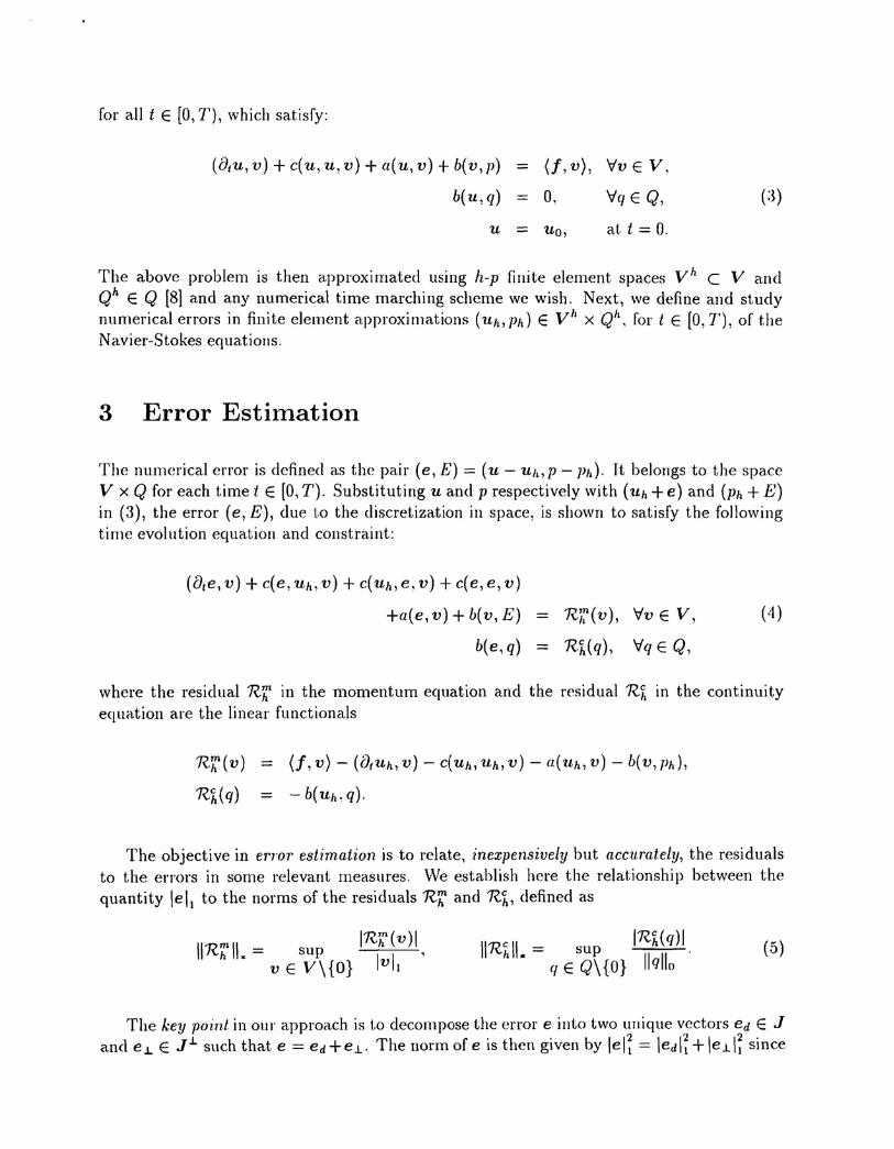
The above error control strategy is tested on the simulation of channel flow past a cylinder.It is well-known that such a flow develops into a periodic vortex shedding as it becomesunstable to unsymmetric perturbations past a critical value of the Reynolds number. Theflow domain n is initially discrctized into the 160-element mesh shown in Figure 1. Thecylinder is slightly moved off-center in order to generate unsymmetric perturbations. TheReynolds number is defined as He = Ucd/v where d is the diameter of the cylinder andUc the maximal velocity of the parabolic profile at the inflow. We select Re = 100 in thepresent experiment. The basis functions for the velocity and pressure consist in piecewise

::2 0 5 10 15 20

Figure 1: Geometry and initial mesh.

-32

o

(d)

(b)

I'~,

0

·1

tt='/ I! \\~ I !

-1 0 1 2 3

(c)

'~0

.,I)=;'/li~., 0 1 2 3

-~

(a)

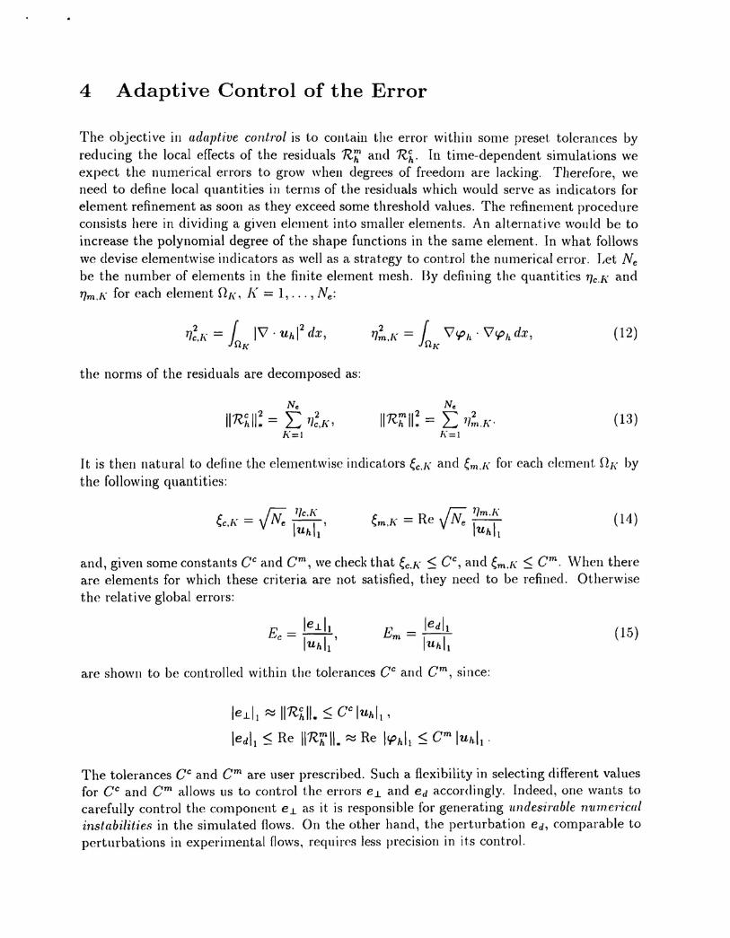
Figure 2: Evolution of the adapted mesh (close-up views around the cylinder)at (a) t = 5 (b) t = 25 (c) t = 50 (d) t = 200.

biquadratic and bilinear functions respectively. The numerical solution is advanced in tirneusing the Adams-Bashforth Cranck-Nicolson scheme (ABCN). The dimensionless timestep isfixed to the value D.l = 0.01 so that the errors due to the time discretization are kept sma.ll.Finally, the initial state Uo is chosen as the Navier-Stokes solution computed at He = 1.

We show in Figure 2 the adapted mesh at various times of the simulation. At t = 50,for example, the mesh is made of 532 elements while the final mesh contains 967 elements.'rVe remark, however, that no adaptation was performed in the time period [100,200] as theflow had reached the permanent periodic regime. The tolerances Ce and Cm are chosen asfunctions of time in order to allow for larger numerical errors during the transients. Theestimated relative global errors Ee and Em, given in (15), are eventually reduced to about5% a.nd 10.5% respectively. The evolution of the tolerances and relative errors is shown inFigure 3. In comparison, the estimated global errors grow very fast during the transients andstabilize around 15% and 55%, when the numerical solution is calculated on the initial meshwithout performing any error control, i.e. without mesh adaptation, as shown in Figure 3.

200150

Em with error control -Ec with error control _Uno

Em w/o error control .Ec w/o error conlrol .

100Time (s)

50

............ ----.--- ...--.-...-------- ...... - --- ---------- -..---- ..oo

0.2

0.8

1.2

0.4 J:.! - ..0.6

200150

Relative error Em -Tolerance Cm -----

Relative error Ec ..Tolerance Cc ..n .

100Time (s)

50

,,,,-,

'-,~:-,

'-,.....~ '. ---- .... -- ----- -- - ....... - -- ------ .. P"

0.2

1.2

0.8

Figure 3: Time evolution of the tolerances Ce and em and estimated rela.tiveerrors Ec and Em with and without error control.

2.301 2.3054

2.3 2.3052

~ ~or or:£ :£

2.299 2.305

2.298 2.30482.298 2.299 2.3 2.301 23048 2305 2.3052 2.3054

Ke(t) Ke(t)

Figure 4: Phase portraits (left) with error control (right) without error control.

In addition, we use the time delay reconstruction technique to create phase portraitsbased on the global kinetic energy signal /(e(t). Tn Figure 4, we show the phase portraits [or

the numerical solutions calculated with error control (left) and without error control (right).They reveal that the solution obtained with error control is periodic with time, as expected,whereas the solution obtained on the initial mesh with no a.da.ptation clearly converges to asteady-state regime. This confirms that it is essential to control the quality of the spatialdiscretization in order to capture the right dynamical flow properties.

6 Conclusion

vVe have proposed a fully automatic adaptive strategy for the control of t.he numerical errorfor the time-dependent. Navier-Stokes equations. It. has been successfully tested on the simu-lation of a channel flow past a cylinder in the periodic regime, for which a numerica.l solutionhas been controlled within some preset error tolerances. The proposed error estimation andadaptive strategy methods a.re nevertheless applicable to flows at any given Reynolds num-ber and work is currently in progress to utilize them for direct numerical simulations of flowtransition and turbulence.

Acknowledgement. The support of this work by the Office of Na.val Research undercontract N00014-95-1-0401 is gra.tefully acknowledged.

References[1] I. Babuska and W. Rhcinboldt, "A posteriori error estimates for the finite element method." Int. J. JOI'

Num. Meth. in Eng .. vo\. 12, pp. 1597-lG15, 1978.

[2] J. T. aden, W. Wu, and M. Ainsworth, "An a posteriori error estimate for finite element approximationsof the Navier-Stokes equations," Compo Meth. in Appl. Mec/1. and EII9., vol. 111, pp. 185-202,1993.

[3] R. Verfiirth, "A posteriori error estimators for the Stokes equations," Numer. Math .. vol. 55, pp. 309-325,1989.

[4] R. E. Bank and B. D. Welfert, "A posteriori error estimates for the Stokes problem," SIAM J. Numer·.Anal., vol. 28, pp. 591-623, 1991.

[5] .I.-F. Hetu and D. H. Pelletier, "Fast, adaptive finite element scheme for viscous incompressible flows,"AIAA JOIJ1'lI(lI, va\. 30, 1992.

[6] R. Verfiirth, A Review of A posteri01·j Error Estimation and Adaptive Mesh-refinement Techniques.Wiley-Teubner, 1996.

(7] V. Girault and P.-A. Raviart, Finite Element Methods Jor Navier-Stokes Equations. Springer-Verlag.1986.

[8] J. T. aden. L. Demkowicz, W. Hachowicz, and O. Hardy. "Toward a universal h-p adaptive finite elementstrategy. Part 1: Constrained approximation and data st.ructure," Comp. Meth. in Appt. J\Jech. and Eng.,vo\. 77, pp. 113-180, \989.

(9] C. R. Doering and J. D. Gibbon, Applied Analysis of the Navier-Stokes Equations. Cambridge UniversityPress, 1995.