Adapting Guidance Methodologies for Trajectory Generation ...
88
Adapting Guidance Methodologies for Trajectory Generation in Entry Shape Optimization
Transcript of Adapting Guidance Methodologies for Trajectory Generation ...

Adapting Guidance Methodologies for Trajectory Generation in Entry Shape
Optimization

Motivation
2
Flight Feasible Trajectories will
Model Realistic In-Flight Thermal States:
• Allow for increased accuracy in Thermal Protection System sizing
(potential mass savings)
• Reduce the number of design cycles required to close an entry
spacecraft design (potential cost savings)

Novel Research Objective
3
Develop a planetary guidance algorithm that is adaptable to:-Mission Profiles-Vehicle Shapes
Alti
tude
Time
Mission Profiles
Vehicle Shapes
Develop a planetary guidance algorithm that is adaptable to:-Mission Profiles-Vehicle Shapes
Develop a planetary guidance algorithm that is adaptable to:-Mission Profiles-Vehicle Shapesfor integration into vehicle optimization. Skip
Loft
Direct

4
Sample Concept of Spaceflight Operations* Adapted graphic from NASA Johnson Space Center
Launch to:• Earth Orbit• Planetary Body
Exploration:Vehicle completes mission over several day or weeks
De-Orbit Separation
Atmospheric Entry
Descent
Landing
De-Orbit
EDL

Planetary Entry Spacecraft Design (cont’d)
5
L
– variable bank angle fixed angle of attack
Mid - Low L/D Spacecraft
High L/D Spacecraft
L
– variable bank angle variable angle of attack
* Space ShuttleAIAA 2006-659
* NASPAIAA 2006-8013
* HL-20AIAA 2006-239
* Orion Capsulewww.nasa.gov
* MSL CapsulePrakash et al., NASA JPL
* EllipsledGarcia et al.,AIAA Conf. Paper

Multi-Disciplinary Design, Analysis, and Optimization
6
(MDAO)
Vehicle Optimization
Entry Trajectory Modeling
Guidance, Navigation, & Control
Flight Feasible Trajectory Database
(replace Traj. Opt.)
Aerodynamic (CD, CL) & Aerothermodynamic ( ) Databases
Decoupled IterationsDecoupled
Iterations
Planetary Models
Un/manned
Available Descent Technologies
Computer Generated Spacecraft Models
Thermal Protection System (TPS) Sizing
Structures
Coupled q
Minimize:Heat Rate (Trajectory/Shape)Ballistic Coefficient (Shape)
Mission Profile

Trajectory Optimization vs. Guidance
7
Trajectory Optimization Guidance
Constraints Multiple included Minimal included
Objective Any variable of interest Target specific
Solution Purely numerical Combination of numerical and analytical
Time to Solution Minutes to hours Seconds
Guaranteed Solution No Must enforce that a solution is found
Parameter Changes Handles large parameter changes
Handles parameter changes that are relatively small
Result Nominal Trajectory – not always realistic control
Flight Feasible Trajectory with realistic controls

Guidance Development Trade-Offs
8
Adaptability Numerical formulation for adaptability to different vehicles and missions
without significant changes
Rapid Trajectory Generation Analytical driving function keep time to a solution low
Minimize Range Error & HeatloadOptimal Control theory to introduce heat load as an additional objective
Guidance Development Criteria
9
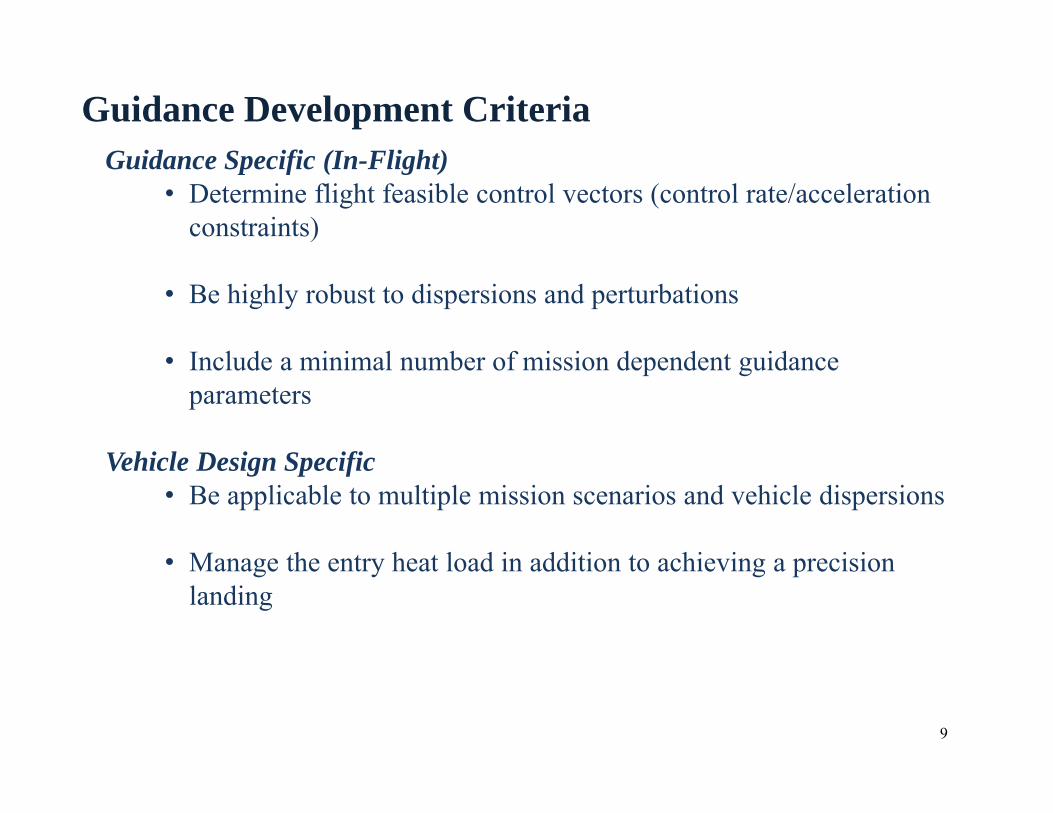
Guidance Specific (In-Flight)• Determine flight feasible control vectors (control rate/acceleration
constraints)
• Be highly robust to dispersions and perturbations
• Include a minimal number of mission dependent guidance parameters
Vehicle Design Specific • Be applicable to multiple mission scenarios and vehicle dispersions
• Manage the entry heat load in addition to achieving a precision landing

Types of Guidance Techniques
10
Reference Tracking Only – follow a pre-defined track
In-flight Reference Generation & Tracking – Generate a real-time reference trajectory and follow that track
In-flight Controls Search – One dimensional search, usually solving equations of motion numerically
In-flight Optimal Control – Requires numerical methods to meet some cost function

Types of Guidance Formulations
11
Analytical Guidance Numerical Guidance
Advantages• Simple to Implement• Computation time minimal• Solution Guaranteed
• Accurate trajectory solutions• No simplifying assumptions
(possibility of multiple entry cases to be simulated with few modifications)
Disadvantages
• Simplifications reduce accuracy of the trajectory solution
• Formulation tied to a specific entry case
• Convergence is not assured• Convergence is not timely

Novel Approach to Guidance for MDAO
12
Adaptability Numerically solve entry equations of motion
Use generalized analytical functions to represent the reference
Rapid Trajectory Generation Use analytical driving function keep time to a solution low
Use Single Optimal Control Point with Blending
Minimize Range Error & HeatloadOptimal Control theory used to introduce heat load objective
Real-Time Trajectory Generation and Tracking
Adaptation of Shuttle Entry Guidance Techniques
Adaptation of Energy State Approximation Techniques

Skip Entry Critical Points
13
Begin with 1st Entry portion of the trajectory and gradually includes remaining phases.
Test Case: Orion Capsule, L/D 0.4
Control: Bank Angle only

Trajectory Simulation Validation
14
Open Loop Simulation (MATLAB)Open Loop Reference (SORT)Closed Loop Simulation (MATLAB)Closed Loop Reference (SORT)
Simulation of Rocket Trajectories (SORT) Developed by NASA Johnson Space Center for Space Shuttle Launch/Entry Simulations
Truth Model

Flight Dynamics
15
rV
V Vproj
V
LD
xb
zb
XECF
YECF
ZECF
Horizontal Plane Diagrams
ECF – Earth Centered Fixed
- longitude - latitude - flight path angle - azimuth
b – body fixed coordinate
Horizon
L
– bank angle
Landing Site

Trajectory Modeling
16
rV
rVVr
coscoscos
sincossin
cossinsincos
sincoscostan2tansincoscossin1
sincossincoscoscossincos2coscos1cossincoscossincossin
22
22
2
rVr
VLV
rVgr
VLV
rgDV
State Variables r - radial distanceV - relative velocity - longitude - latitude - flight path angle - azimuth
Vehicle and Planet VariablesL, D - Lift, Drag Accelerationg - gravity - Earth‘s Rotation – atmospheric density
Control Variables - bank angle - angle of attack

General Entry Guidance Block Diagram
17
Trajectory SolverReference Trajectory: Analytical functions adapted from Shuttle Entry GuidanceBank Schedule Solution: Range Prediction: numerically solve equations of motion, range calculation
Rerr ~= 0
No
Yes
Targeting Algorithm
Solver: Single Point Optimal Control Solution from Energy State Approximation
Purpose: Targeting for precision landing and minimizing heatload
Dispersed State:
Sendto flight simulation
dispy
cmd
cmd
new

18
Shuttle Entry Guidance (SEG) Concept: Temperature Phase• Reference Tracking Algorithm, Closed Form Solution
Control Solution: Shuttle Entry Guidance Adaptation
Reference Trajectory Bank Schedule Solution () Range Prediction
ref = constant
fV
V ref
rr
gDdVVs
1
refref
ref
ref
refref
v Dg
Dg
rV
Vh
Dh
DL 22 1
D
D
ref
refsref C
CVV
DD
hh
2
2
222
VVD
VD
DD
DD
hh refref
ref
ref
ref
refsref
mACVD
dtd Dr
2
2
012
2ref CVCVC D

19
Control Solution: Shuttle Entry Guidance AdaptationImprovements on Shuttle Entry Guidance “Drag Based Approach”•Increase # of segments•Increase order of polynomial•Change Atmospheric Model representation•Modify flight path angle representation
Challenges with Drag Based Approach• Discontinuities between segments• Increasing # of coefficients for storage with increasing segments and/or
order• Effect of small flight path angle assumption unknown• Formulations are derived from 2DOF Longitudinal EOMs

20
Control Module: Shuttle Entry Guidance AdaptationSensitivity to atmospheric non-linearity is significant during initial and final segments. Need an Alternative Analytical Equation!
Reference Trajectory Analytic Bank Angle Control Equation
rref
rrD
refref
V withTable Stored
VCVmACD
22
2
cos
)y(cos1
,
2
,
totalrefv
rrefr
refrefv
DL
DL
Cgr
VVDL
Trajectory ModuleNPC Solves 3DOF EOMs
Controls ModuleDrag and FPA Rate
Reference Trajectories
Range Prediction (R)Great Circle Range
Current State Vectoryo = [r V ]
yii
ytotal
Final Trajectory Solver Approach

Automated Selection of Transition Events
21
Framework:- Allows for adaptability- Automated generation of Reference Trajectory- Open loop
Study Objective: Define bank profile for trajectory phases
Phase Bank DescriptionEntry Interface to
Guidance Start Constant Bank
Guidance Start to Guidance End Trajectory Solver
Guidance End to Exit Linear Transition to Meet 2nd Entry Bank
Exit to 2nd Entry Attitude Hold

Automated Selection of Transition Events
22
• Metric to determine best trajectory: lowest range error, lowest heat load from EI to 2nd Entry, and bank transitions

Automated Selection of Transition Events
23
Study Results:Phase Bank Description
Entry Interface to Guidance Start Constant Bank = 57.95o
Guidance Start to Guidance End Trajectory Solver{0.12 0.11} G’s
Guidance End to Exit Linear Transition to Meet 2nd Entry BankLinear Transition Velocity: 23,784.65 ft/s
Exit to 2nd Entry Bank Attitude Hold = 70o
Guidance StartGuidance End
2nd Entry Bank

General Entry Guidance Block Diagram
24
Trajectory SolverReference Trajectory: Analytical functions adapted from Shuttle Entry GuidanceBank Schedule Solution: Range Prediction: numerically solve equations of motion, range calculation
Rerr ~= 0
No
Yes
Targeting Algorithm
Solver: Single Point Optimal Control Solution from Energy State Approximation
Purpose: Targeting for precision landing and minimizing heatload
Dispersed State:
Sendto flight simulation
dispy
cmd
cmd
new

Targeting Algorithm Development
25
When is Targeting Activated?
1.Overshoot – Vehicle is predicted to fly way past target2.Undershoot – Vehicle is predicted to fly short of the target
How to find a set of controls to Correct Over/Underhoot?
Adapt Energy State Approximation Methods: Optimal control method that replaces altitudeand velocity with specific energy height (e) h
gVe
o
r 2
2
Advantages: Allows for a compact set of analytical equations
Add heat load to the range error objective function
Disadvantage: Optimal control formulations may not converge to a solution
Solution: Derive a localized optimal control point instead and blend back reference trajectory

26
Targeting Algorithm DevelopmentMust Relate Euler-Lagrange Equation
To Reference Trajectory Variables
)(cos1cos
2
yCgr
VVDL r
refrreftotal
Using trigonometry and other manipulations, the control equation isfound

Targeting Algorithm Development
27
2
2 rref
Dref V
mAC
Least Squares Curve Fitting:
3 Interpolation PointsControl Point
dV
Targeting Algorithm Development
28
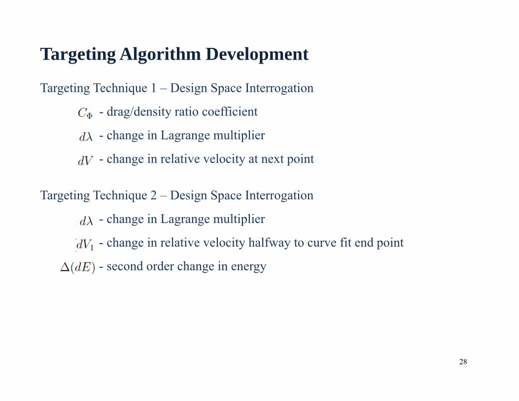
Targeting Technique 1 – Design Space Interrogation
- drag/density ratio coefficient
- change in Lagrange multiplier
- change in relative velocity at next point
Targeting Technique 2 – Design Space Interrogation
- change in Lagrange multiplier
- change in relative velocity halfway to curve fit end point
- second order change in energy

Lower Limit
Upper Limit
Incr. units
0 1 ND
0 1 0.01 ND
100 1000 100 ft/s
Targeting Algorithm Development
29
Targeting Technique 1 – Design Space Interrogation
Case Dispersion Target Miss1 Increase Entry Flight
Path AngleUndershoot
2 Decrease Entry Flight Path Angle
Overshoot
3 L/D Dispersion Overshoot

Targeting Algorithm Development
30
FPA Dispersion - Undershoot

Targeting Algorithm Development
31
FPA Dispersion - Overshoot

Targeting Algorithm Development
32
Aerodynamic Dispersion - Overshoot

Shape Optimization Analog
33
MDAO
Geometry #3: CL = 1.95, CD = 3.9
Geometry #2: CL = 1.90, CD = 3.8
Geometry #1: CL = 1.70, CD = 3.4
ANALOG: Changing angle of attack
disperses CL and CD
Current Guidance Algorithms – Robust to ~20% aerodynamic dispersions
Must exceed 20% to demonstrate potential for integration into MDAO
velocity
+5%
-50%

Targeting Algorithm Development
34
Guidance Algorithm for Comparison – Apollo Derived Final Phase Guidance
Reference Tracking to a stored trajectory database, function of relative velocity
Performance Results – Threshold Miss Distance, 1 nmi

Targeting Algorithm Development
35
Targeting Technique 1 – Targeting Procedure
1. Guess a value for d
2. Iterate on dV using secant method to converge on a zero range error trajectory
3. If no solution is found, d is incremented and the iteration is repeated
4. Solution is then flown in flight simulation
Targeting Algorithm Development
36
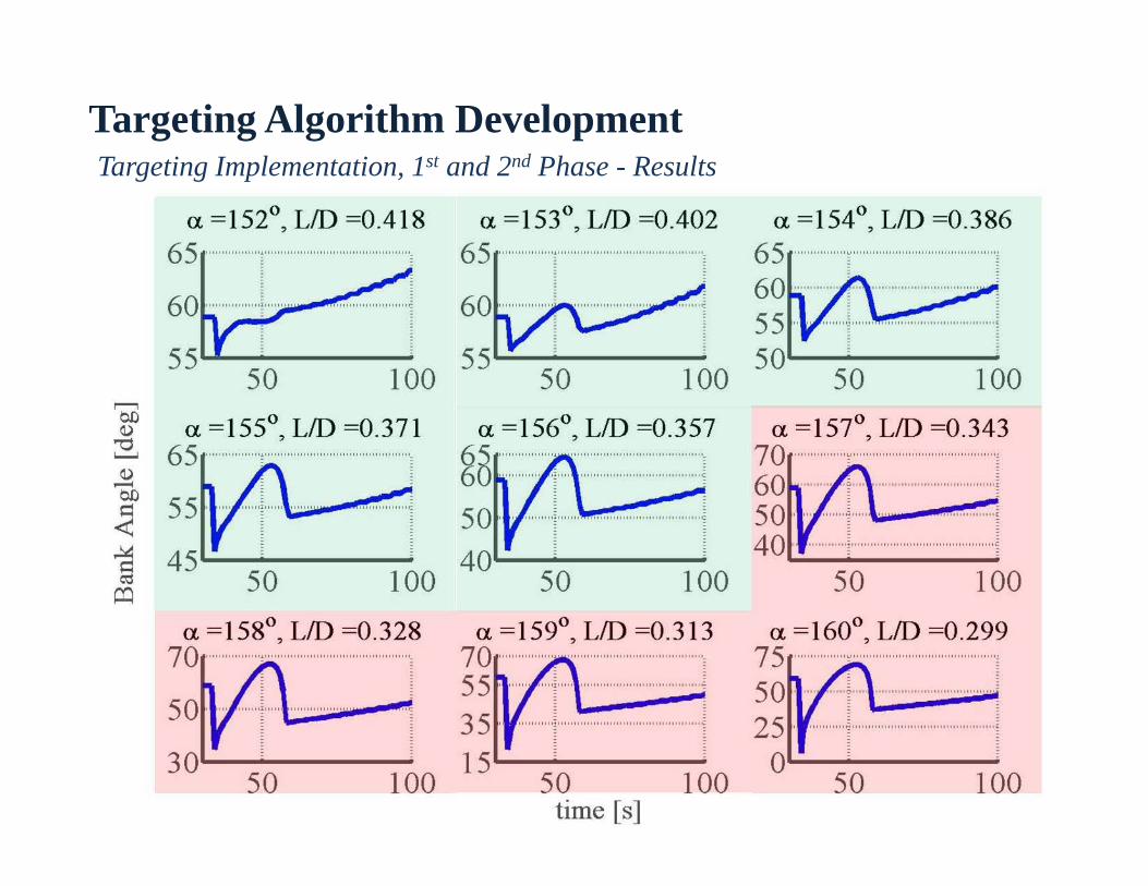
Targeting Implementation, 1st and 2nd Phase - Results

Targeting Algorithm Development
37
Targeting Technique 2
Use Energy Height to determine Control Pointhg
Veo
r 2
2
Undershoot → energy dissipating (de/dt) too fast
Overshoot → energy dissipating (de/dt) too slow
Since Velocity is an independent variable and a pseudo control de/dV is examined

Targeting Algorithm Development
38
Targeting Technique 2Recall the equation for the ratio of drag acceleration to density:
-Extract altitude and velocity from to find
2
2 rD VmACD
new

Targeting Algorithm Development
39
Targeting Technique 2 – Design Space Interrogation
Lower Limit Upper Limit Incr. units0 ND0 1524 Predict m/s0 Predict m
Limit are trajectory dependent and control system dependent
Dispersion Cases:
1st Phase Only [deg] L/D Dispersion Target Miss
Nominal 0.4 (0%)152 0.42 (+5%) Undershoot162 0.28 (-30%) Overshoot165 0.23 (-43%) Overshoot167 0.2 (-50%) Undershoot

Targeting Algorithm Development
40
Design Space Interrogation, Results: Range Error [%] = 152o, Undershoot = 162o, Overshoot
= 165o, Overshoot = 167o, Undershoot
Targeting Algorithm Development
41
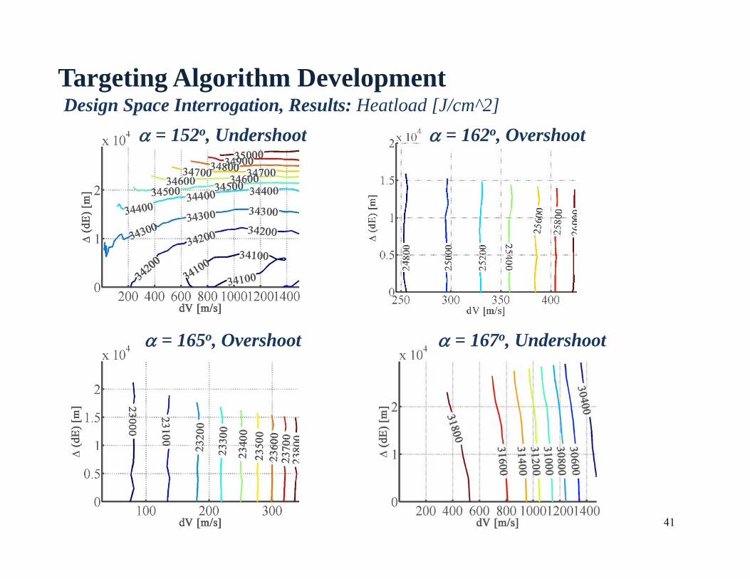
Design Space Interrogation, Results: Heatload [J/cm^2] = 152o, Undershoot = 162o, Overshoot
= 165o, Overshoot = 167o, Undershoot
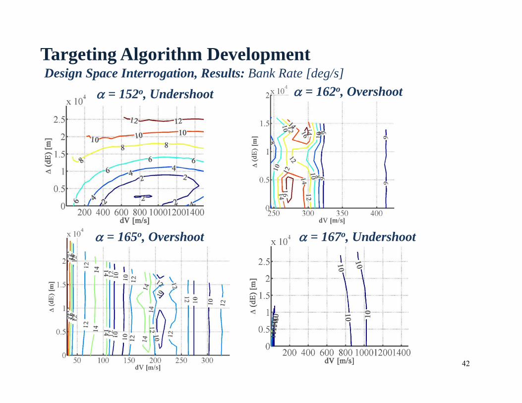
Targeting Algorithm Development
42
Design Space Interrogation, Results: Bank Rate [deg/s] = 152o, Undershoot = 162o, Overshoot
= 165o, Overshoot = 167o, Undershoot

Targeting Algorithm Development Results
43
Dispersions –
Apollo Derived Guidance = -20% dispersion
MDAO Algorithm = -43% dispersion
Managing heatload may be a challenge for dispersions greater than 20%
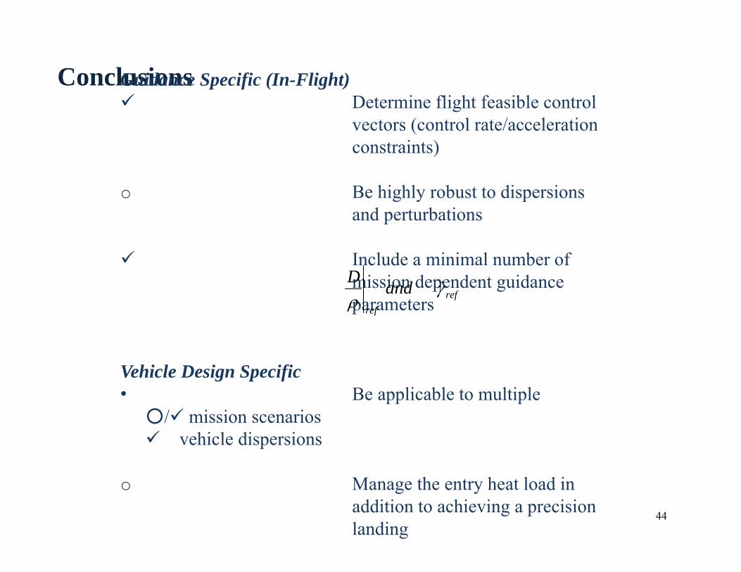
Conclusions
44
Guidance Specific (In-Flight) Determine flight feasible control
vectors (control rate/acceleration constraints)
o Be highly robust to dispersions and perturbations
Include a minimal number of mission dependent guidance parameters
Vehicle Design Specific • Be applicable to multiple
○/ mission scenarios vehicle dispersions
o Manage the entry heat load in addition to achieving a precision landing
refref
andD

45
AcknowledgemetsUniversity of California, Davis
Dr. Nesrin Sarigul-KlijnDissertation Chair
Dr. Dean KarnoppDissertation Committee Member
UC Davis Mechanical and Aerospace Engineering Faculty
UC Davis Mechanical and Aerospace Engineering Staff
NASA Ames Research Center
Dr. Dave KinneyDissertation Committee Member
Mary LivingstonSupervisor
Colleagues in Systems Analysis Office
Thank You !!!

Questions?
46

Additional Slides(optional)
47

Overview
48
Background & Motivation Elements of Spacecraft Design
Introduction to Planetary Entry Guidance
Dissertation Research Plan and Status
MAPGUID Development MAPGUID Proposed Approach
Key Results #1
Key Results #2
Key Results #3
Key Results #4
Aerothermal ManagementDuring Guidance
Proposed Approach
Key Results #1
Key Results #2
Guidance/COBRAIntegration
Proposed ApproachKey Results #1
Key Results #2
Key Results #3
Closing Remarks Dissertation Findings and Status

Big Picture:Spacecraft Design Process
49

MDAO Literature Review
50
Vehicle Optimization and TPS Sizing
Example Objective Function:
Results
• Most studies use a single trajectory to find altitude-velocity corresponding to
maximum heat rate
• Used for all geometries within optimization to find heat rate
• Some studies use new trajectories, but there is no accounting for bank constraints or
target accuracy
• None of these studies incorporated flight feasible trajectories
What is Flight Feasible?
• Reaches Target @ Landing Speeds
• Control does not exceed system limits

Proposed Approach to MDAO for Spacecraft Design
51
Vehicle Optimization
Planetary Entry Guidance
Guidance, Navigation, & Control
Flight Feasible Trajectory Database
Aerodynamic (Cd, CL) & Aerothermodynamic ( ) Databases
Reduced Decoupled Iterations
Reduced Decoupled Iterations
Thermal Protection System (TPS) Sizing
Structures
Coupled
Planetary Models
Un/manned
Available Descent Technologies
Computer Generated Spacecraft Models
Mission Profile

Trajectory Modeling for Design vs. In-Flight Trajectory Modeling
52

Planetary Entry Guidance Literature Review
53
• High L/D, Earth: Space Shuttle, X-33, X40A
• Most Robust: In Flight Trajectory Shaping with Reference
Tracking
• Least Robust: Reference Tracking Only
• Low L/D, Earth: Apollo, Orion
• Most Robust: In-Flight Controls Search
• Least Robust: Reference Tracking Only
• Other Planetary Entry Vehicles: MSR, MSL, Biconic
• Flight Tested algorithms preferred

Planetary Entry Guidance Literature Review (cont’d)
54
Robust guidance algorithms: combo of numerical and analytical approaches
Key Results
Least robust algorithms: purely analytical solutionsAdaptability of guidance algorithms: very little among all algorithmsModern guidance algorithms: optimal control is potential framework, but
convergence still an issueHeat load management: not included

Trajectory Optimization Literature Review
55
Trajectory Optimization
Traj - Nonlinear constrained optimization
Mission - Sequential Quadratic Programming
Energy State Method – Reduced Order Modeling, one dimensional
parameter search
Pseudospectral Methods – Combination indirect and direct
method, mapping and discretization of domain

Trajectory Optimization Literature Review (cont’d)
56
Curse of dimensionality: Convergence time increases with dimensionality
Key Results
No convergence to a solutionFidelity of modeling may be compromised

Introduction to Planetary Entry Guidance
57

Guidance Development Process
58
*Guidance must be robust to many dispersions:(Atmospheric properties, Aerodynamics properties, Navigational Inputs, Entry Interface Conditions, Mass, Control System performance, and many others)

Baseline Vehicle & Mission
59

Case Study Parameters
60
Vehicle Orion Capsule, L/D = 0.4
Trajectory Skip Entry for Lunar Return
Control Bank Angle only
Atmospheric Model 1976 Standard Atmosphere
Gravity Model Central Force + Zonal Harmonics
Aerodynamics CL, CD corresponding to Mach #
CBAERO Databases, function of Mach #, Dynamic Pressure, and Angle of Attack
Trajectory Simulation MATLAB Simulation validated against SORT Trajectories

Trajectory Simulations Developed
61
3DOF Rotating Spherical Planet
rV
rVVr
coscos
cossincossin
cossinsincos
sincoscostan2tansincoscossin1
sincossincoscoscossincos2coscos1cossincoscossincossin
22
22
2
rVr
VLV
rVgr
VLV
rgDV
Flight Simulation - Closed Loop Guidance TestingUsing equations derived from Newton’s 2nd Law, dynamics of relative motion, and Earth Centered Inertial (ECI) coordinate system
Open Loop Numerical Predictor- Corrector (NPC) SimulationUsed to test guidance formulations

Trajectory Solver Development
62

63
Control Solution: Shuttle Entry Guidance AdaptationDrag Curve Fit Accuracy
Segments Order # of stored coefficients
7 (3) Irrational 1681058421
7 (5) Irrational14 57 2
012 x0
x1
x2ref VCVCVC D

64
Control Solution: Shuttle Entry Guidance AdaptationWould Cubic Spline Interpolation work?

Targeting Algorithm Development
65

Targeting Algorithm Development
66
Targeting Technique 1 – Trajectory Behavior to Full Set of Aerodynamic Dispersion
Can Technique 1 find a trajectory that points toward correcting the range error?

General Conclusions
67

Euler-Lagrange Equation
The optimal control satisfies several constraints including the Euler-Lagrange Equation:
68
Targeting Algorithm DevelopmentPontryagin’s Principle in Optimal Control
Find Optimal Control
for dynamic system

Targeting Algorithm Development
69
Targeting Technique 1
→ new→
→
→
Determines new bank angle at current time step
Calibrated for Each Dispersed Case
Determines Blended Trajectory that nulls range error

Targeting Algorithm Development
70
Targeting Technique 1 – Design Space Interrogation
• The blending technique exhibits potential to find new bank profiles that null the range error
• The design space is constrained by control system limitations
• There is a zero range error solution for each change in d
Targeting Algorithm Development
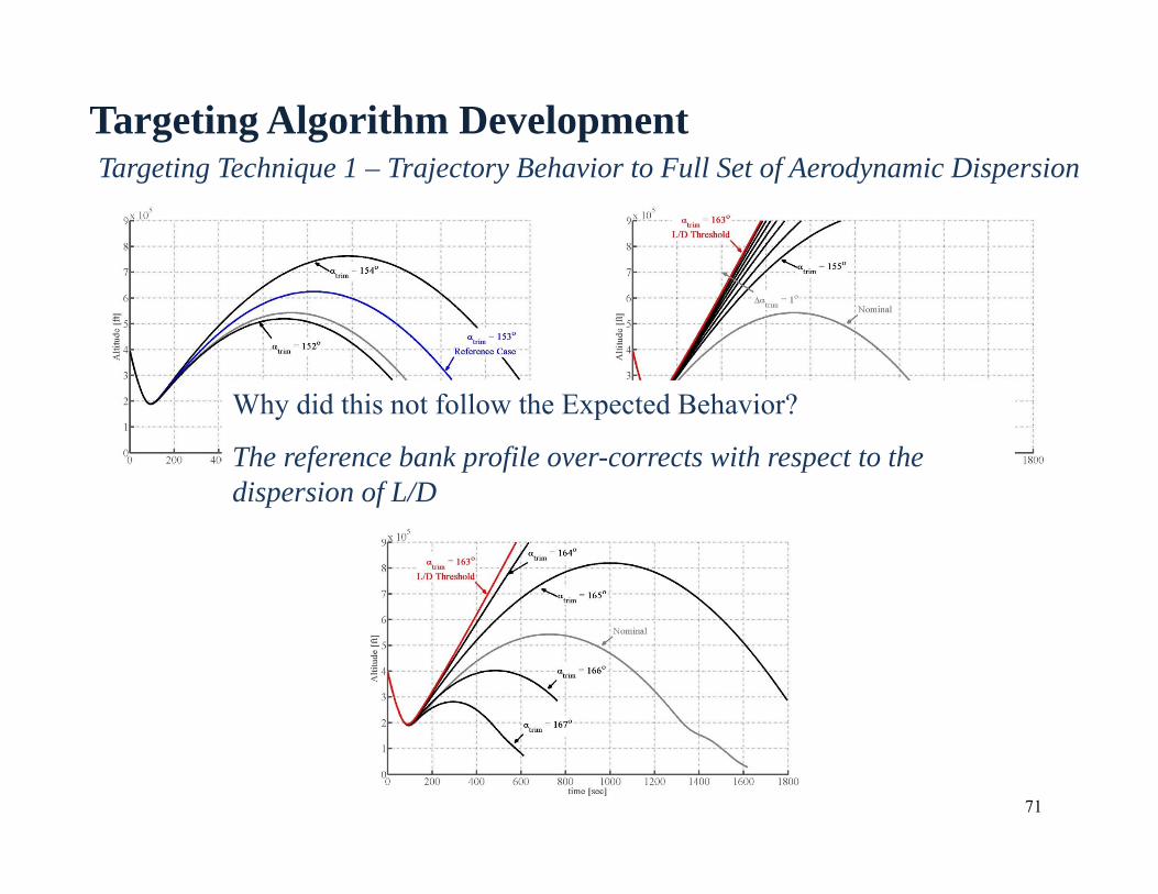
71
Targeting Technique 1 – Trajectory Behavior to Full Set of Aerodynamic DispersionExpected Behavior –
Increasing angle of attack causes an UndershootDecreasing angle of attack causes an Overshoot
Why did this not follow the Expected Behavior?
The reference bank profile over-corrects with respect to the dispersion of L/D

Targeting Algorithm Development
72
Targeting Technique 2Now that the blended function is fully defined
The following equation can be used to solve for:
The FPA rate table is shifted accordingly

Targeting Algorithm Development
73
Design Space Interrogation, Results: Bank Acceleration [deg/s^2] = 152o, Undershoot = 162o, Overshoot
= 165o, Overshoot = 167o, Undershoot

Targeting Algorithm Development
74
Targeting Technique 1 – Targeting Implementation, 1st and 2nd Phase
1. Guess a value for d
2. Iterate on dV using secant method to converge on a zero range error trajectory
3. If no solution is found d is incremented and the iteration is repeated
4. Solution is then flown in flight simulation
Performance Metric –
Compare range of aerodynamic dispersions this algorithm can handle to the range of aerodynamic dispersions a heritage algorithm can handle.
Trajectory Solver Research Questions
75
Can a simplification in the equations of motion be made without loss of accuracy?
Can a simplification on flight path angle be made without loss of accuracy?

Simplified Equations of Motion Study
76
3DOF Rotating , Spherical Earth (3RSP)
cossinsin
cos)sincoscos(tan2tansincos
cossin1 22 rV
rVL
V
tansincos
cossin1 2
rVL
V
cossin1 L
V
gr
VLV
gDVVsVh
2
coscos1sin
cossin
Apollo and Shuttle Entry Guidance
3DOF Non-Rotating Spherical Planet
3DOF Non-Rotating Flat Planet
2DOF Longitudinal Equations (2LON)
Coriolis and CentripetalAcceleration

Simplified Equations of Motion Study (cont’d)
77
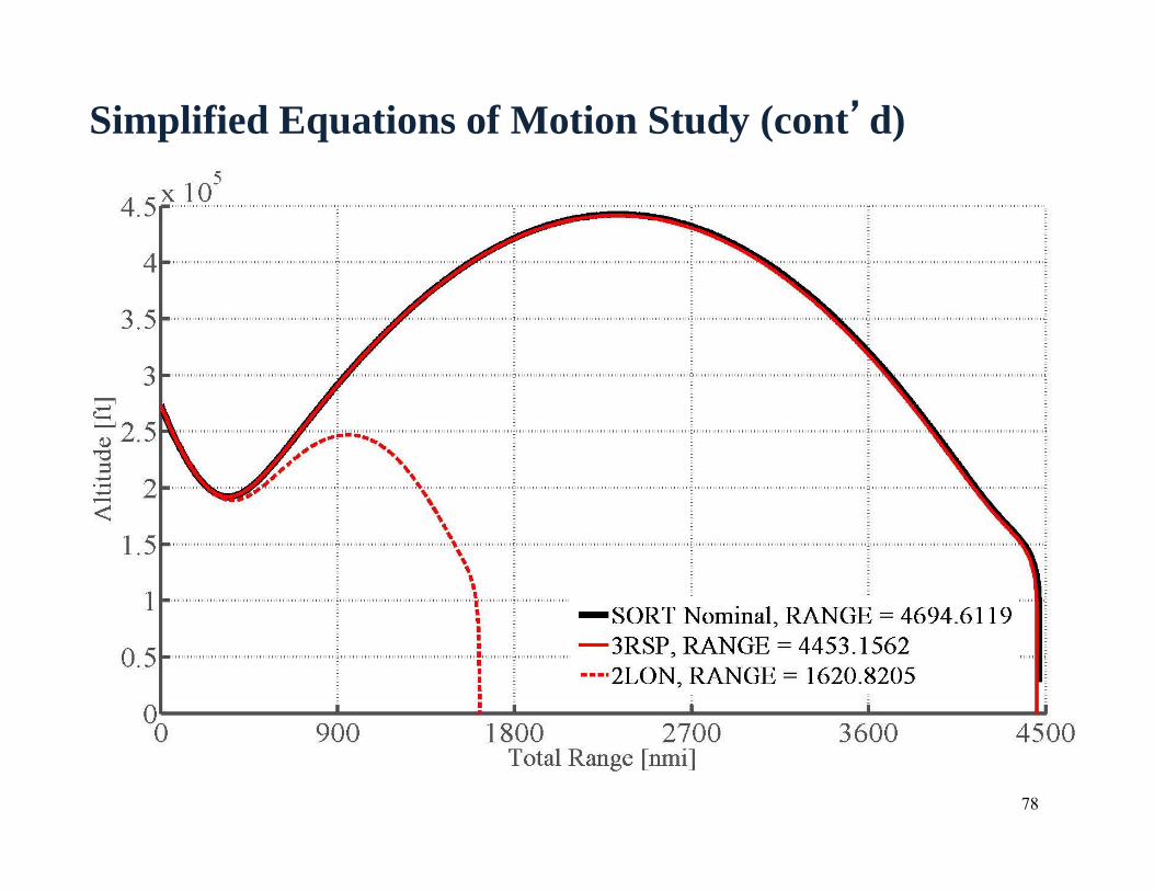
Simplified Equations of Motion Study (cont’d)
78

Trajectory Solver Research Questions
79
Can a simplification in the EOMs be made without loss of accuracy? Not for a skip trajectory
Can a simplification on flight path angle be made without loss of accuracy?

80
Control Solution: Shuttle Entry Guidance Adaptation
D
D
ref
refsref C
CVV
DD
hh
2

81
Control Solution: Shuttle Entry Guidance Adaptation

82
Control Solution: Shuttle Entry Guidance Adaptation

83
Control Solution: Shuttle Entry Guidance AdaptationNeed to Resolve 1st Segment to Capture Atmospheric Non-LinearityIDEA: Curve fit drag with Mach Number
n
1i
iiref aMC D

84
Control Solution: Shuttle Entry Guidance AdaptationCheck Altitude Acceleration Approximation

Trajectory Solver Research Questions
85
Can a simplification in the EOMs be made without loss of accuracy? Not for a skip trajectory
Can a simplification on flight path angle be made without loss of accuracy?

Range Prediction Sensitivity to Flight Path Angle Assumption
86
• Apollo and Shuttle Entry guidance formulations approximate flight path angle (FPA) to be small:
sradrad /1and/or1
Why does this matter?• If predicted range does not equal the range to landing site then targeting is
erroneously active• Are model reductions in the Trajectory Module and Control Module valid
based on the nominal case?

Range Prediction Sensitivity to Flight Path Angle Assumption
87
Trajectory ModuleNPC Solves 3DOF EOMs
Controls ModuleDrag and FPA Rate
Reference Trajectories
Case Studies:A. Apply to Trajectory
Module only
B. Apply to Controls Module only
C. Apply to bank equation only
)y(cos1 2
,
Cg
rVV
DL r
refrrefrefv
rad1
srad /1
rad1

Range Prediction Sensitivity to Flight Path Angle Assumption
88
Nominal 661.73 [nmi]
Case Total Range [nmi] % Range Error TerminationA 662.39 0.099% Drag LimitB 649.74 1.813% Drag LimitC 632.13 4.474% Velocity Limit
Conclusion FPA approximation can be applied to the trajectory module, but not to the control module