Adaptation techniques to improve ASR performance on ...

Adaptation techniques to improve ASRperformance on accented speakers

Udhyakumar Nallasamy

CMU-LTI-16-012

Language Technologies InstituteSchool of Computer ScienceCarnegie Mellon University

5000 Forbes Avenue, Pittsburgh, PA 15213www.lti.cs.cmu.edu

Thesis Committee:Florian Metze Chair,

Tanja Schultz Co-Chair,Alan W. Black,

Monika Woszczyna, M*Modal Inc.

Submitted in partial fulfillment of the requirementsfor the degree of Doctor of Philosophy

in Language and Information Technologies

Copyright c© 2016 Udhyakumar Nallasamy

Abstract

Speech interfaces are becoming pervasive among the common pub-lic with the prevalence of smart phones and cloud-based computing.This pushes Automatic Speech Recognition (ASR) systems to handle awide range of factors including different channels, noise conditions andspeakers with varying accents. State-of-the-art large vocabulary ASRsperform poorly when presented with accented speech, that is eitherunseen or under-represented in the training data. This thesis focuses onproblems faced by accented speakers with various ASR configurationsand proposes several adaptation techniques to address them.

The influence of accent is examined in three different ASR setupsincluding accent dependent, accent independent and speaker dependentmodels. In the case of accent dependent models, a source ASR trainedon resource-rich accent(s) is adapted to a target accent using a limitedamount of training data. Semi-continuous decision tree based adaptationis proposed to efficiently model contextual phonetic changes betweensource and target accents and its performance is compared against tradi-tional techniques. Active and semi-supervised learning techniques thatcan exploit the contemporary availability of extensive, albeit unlabeleddata resources are also investigated.

In accent independent models, a novel robustness criterion is in-troduced to evaluate the impact of accent in various ASR front-endsincluding MFCC and Bottle-neck features. Accent questions are intro-duced in addition to phonetic ones, to measure the ratio of accent modelsin the ASR contextual decision tree. Accent aware training is also pro-posed in the context of deep bottle-neck front-end to derive canonicalfeatures robust to accent variations.

Finally, problems faced by accented speakers in speaker-dependentASR models is addressed. Several neighbour selection and adaptation al-gorithms are proposed to improve the performance of accented speakersusing only a few minutes of data from the target speaker. Extensive anal-ysis is performed to measure the influence of accent in the neighboursselected for adaptation. Neighbour selection using textual features andlanguage model adaptation using neighbours data is also investigated.

Contents

I Introduction 1

1 Introduction 3

1.1 Accent variations . . . . . . . . . . . . . . . . . . . . . . . . . . . . . 3

1.2 Related work . . . . . . . . . . . . . . . . . . . . . . . . . . . . . . . 4

1.3 Thesis contributions . . . . . . . . . . . . . . . . . . . . . . . . . . . 6

1.4 Thesis organization . . . . . . . . . . . . . . . . . . . . . . . . . . . . 7

II Accent dependent modeling 9

2 Target accent adaptation 11

2.1 Related work . . . . . . . . . . . . . . . . . . . . . . . . . . . . . . . 12

2.2 PDT adaptation . . . . . . . . . . . . . . . . . . . . . . . . . . . . . . 12

2.3 Semi-continuous PDT adaptation . . . . . . . . . . . . . . . . . . . . 13

2.4 CMU setup - speech corpus, language model and lexicon . . . . . . . 15

2.5 Baseline systems . . . . . . . . . . . . . . . . . . . . . . . . . . . . . 16

2.6 Accent adaptation experiments . . . . . . . . . . . . . . . . . . . . . 18

2.7 M*Modal setup - speech corpus, language model and lexicon . . . . 21

2.7.1 Database . . . . . . . . . . . . . . . . . . . . . . . . . . . . . 21

2.7.2 Baseline . . . . . . . . . . . . . . . . . . . . . . . . . . . . . . 22

2.8 Summary . . . . . . . . . . . . . . . . . . . . . . . . . . . . . . . . . 24

v

vi CONTENTS

3 Extensions to unlabelled data 25

3.1 Active learning . . . . . . . . . . . . . . . . . . . . . . . . . . . . . . 25

3.1.1 Active learning for accent adaptation . . . . . . . . . . . . . . 26

3.1.2 Uncertainty based informativeness criterion . . . . . . . . . . 27

3.1.3 Cross-entropy based relevance criterion . . . . . . . . . . . . 27

3.1.4 Score combination . . . . . . . . . . . . . . . . . . . . . . . . 30

3.1.5 Experiment setup . . . . . . . . . . . . . . . . . . . . . . . . . 31

3.1.6 Implementation details . . . . . . . . . . . . . . . . . . . . . . 32

3.1.7 Active learning results . . . . . . . . . . . . . . . . . . . . . . 34

3.1.8 Analysis . . . . . . . . . . . . . . . . . . . . . . . . . . . . . . 35

3.2 Semi-supervised learning . . . . . . . . . . . . . . . . . . . . . . . . 37

3.2.1 Self-training . . . . . . . . . . . . . . . . . . . . . . . . . . . . 39

3.2.2 Cross-entropy based data selection . . . . . . . . . . . . . . . 39

3.2.3 Implementation details . . . . . . . . . . . . . . . . . . . . . . 40


3.3 Summary . . . . . . . . . . . . . . . . . . . . . . . . . . . . . . . . . 46

III Accent robust modeling 47

4 Robustness analysis 49

4.1 Related work . . . . . . . . . . . . . . . . . . . . . . . . . . . . . . . 49

4.2 Accent normalization or robustness . . . . . . . . . . . . . . . . . . . 50

4.2.1 Decision tree based accent analysis . . . . . . . . . . . . . . . 50

4.3 Accent aware training . . . . . . . . . . . . . . . . . . . . . . . . . . 51

4.4 Experiments . . . . . . . . . . . . . . . . . . . . . . . . . . . . . . . . 53

4.4.1 RADC setup . . . . . . . . . . . . . . . . . . . . . . . . . . . . 53

4.4.2 M*Modal setup . . . . . . . . . . . . . . . . . . . . . . . . . . 60

4.5 Summary . . . . . . . . . . . . . . . . . . . . . . . . . . . . . . . . . 64

CONTENTS vii

IV Speaker dependent modeling 67

5 Speaker dependent ASR and accents 69

5.1 Motivation for SD models . . . . . . . . . . . . . . . . . . . . . . . . 69

5.2 Accent issues in SD models . . . . . . . . . . . . . . . . . . . . . . . 72

5.3 Related work . . . . . . . . . . . . . . . . . . . . . . . . . . . . . . . 72

5.3.1 Subspace based speaker adaptation . . . . . . . . . . . . . . . 73

5.3.2 Speaker clustering . . . . . . . . . . . . . . . . . . . . . . . . 74

5.3.3 Speaker selection . . . . . . . . . . . . . . . . . . . . . . . . . 75

5.4 Neighbour selection and adaptation . . . . . . . . . . . . . . . . . . . 76

6 Maximum likelihood neighbour selection and adaptation 77

6.1 Neighbour selection . . . . . . . . . . . . . . . . . . . . . . . . . . . 77

6.2 Experiments . . . . . . . . . . . . . . . . . . . . . . . . . . . . . . . . 78

6.2.1 Varying number of neighbours . . . . . . . . . . . . . . . . . 80

6.2.2 Varying the amount of adaptation data . . . . . . . . . . . . . 81

6.2.3 Varying target speaker’s data . . . . . . . . . . . . . . . . . . 82

6.3 Analysis . . . . . . . . . . . . . . . . . . . . . . . . . . . . . . . . . . 83

6.3.1 Influence of gender and accent . . . . . . . . . . . . . . . . . 83

6.3.2 Automatic selection vs. manual annotations . . . . . . . . . . 84

6.4 Unsupervised adaptation . . . . . . . . . . . . . . . . . . . . . . . . . 86

6.5 Summary and discussion . . . . . . . . . . . . . . . . . . . . . . . . . 88

7 Discriminative neighbour selection and adaptation 91

7.1 Discriminative training of SI model . . . . . . . . . . . . . . . . . . . 92

7.2 Discriminative neighbour adaptation . . . . . . . . . . . . . . . . . . 93

7.3 Discriminative neighbour selection . . . . . . . . . . . . . . . . . . . 95

7.4 Deep bottle-neck features . . . . . . . . . . . . . . . . . . . . . . . . 96

7.5 DBNF neighbour selection and adaptation . . . . . . . . . . . . . . . 97


viii CONTENTS

8 Text based neighbour selection 99

8.1 Textual features for neighbour selection . . . . . . . . . . . . . . . . 99


8.1.2 Experiments . . . . . . . . . . . . . . . . . . . . . . . . . . . . 101

8.2 Language model adaptation . . . . . . . . . . . . . . . . . . . . . . . 102

8.3 Analysis . . . . . . . . . . . . . . . . . . . . . . . . . . . . . . . . . . 103

8.4 ASR experiments . . . . . . . . . . . . . . . . . . . . . . . . . . . . . 104


V Conclusion 107

9 Summary and Future Directions 109

9.1 Thesis contributions . . . . . . . . . . . . . . . . . . . . . . . . . . . 109

9.2 Future Directions . . . . . . . . . . . . . . . . . . . . . . . . . . . . . 110

Bibliography 113

Part I

Introduction

1

Chapter 1

Introduction

Speech recognition research has made great strides in the recent years and currentstate-of-the-art ASRs scale to large systems with millions of parameters trainedon thousands of hours of audio data. For many tasks such as broadcast newstranscription, the Word-Error Rate (WER) has been reduced to less than 10% fora handful of languages [MGA+06, SSK+09, GAAD+05, HFT+09]. This has ledto increased adoption of speech recognition technology in desktop, mobile andweb platforms for applications such as dictation, voice search [BBS+08], naturallanguage queries, etc. However, these systems suffer high vulnerability towardsvariations due to accents that are unseen or under-represented in the training data[SMB11, NMS12b]. The WER has been to shown to nearly double for mismatchedtrain/test accent pairs in a number of languages such as English [HW97, NMS12b],Arabic [SMB11, NMS12b], Mandarin Chinese [HCC01] or Dutch/Flemish accents[Com01]. Moreover, accent-independent ASRs trained on multiple, pooled accentsachieve 20% higher WER than accent-specific models [SMB11, BMJ12, Com01].

1.1 Accent variations

Human speech in any language, exhibits a class of well-formed, stylized speakingpatterns that are common across members that belong to the same clique. Thesegroups can be characterized by geographical confines, socio-economic class, ethnic-ity or for second-language speakers, by the speakers’ native language. These spokenlanguage patterns can vary in their vocabulary, syntax, semantics, morphology andpronunciation. These set of variations are termed as ’Dialects’ of a language. Accent

3

4 Chapter 1: Introduction

is a subset of dialect variations that is concerned mainly with the pronunciation,although pronunciation can influence other choices such as vocabulary and word-frequency [Wel82, MHu]. Although non-native pronunciations are influenced bythe speakers’ native language, we do not focus on explicitly modeling L2 variationsin this thesis. Pronunciation variations between different accents can be furthercharacterized by

• Phoneme inventory - Different accents can rely on different set of phonemes

• Phonetic realization - The same phoneme can be realized differently in eachaccent

• Phonotactic constraints - The distribution of phonemes can be different

• Lexical distribution - The choice of words can vary between the accents

Speakers of a specific accent express both unique and common speech patternswith members of other accents of the same language. These accent variations canbe represented by contextual phonological rules of the form

L −m+R → s (1.1)

where L represents the left-context, R the right-context, m the phone to betransformed and s the realized phone. Such rules result in changes to canonicalpronunciation including addition, deletion and substitutions of sounds units. [Uni]used such rules in a hierarchical way to convert an accent-independent pronuncia-tion lexicon to a variety of English accents spanning across US, UK, Australia andNew Zealand.

1.2 Related work

The two main approaches for accent adaptation include lexical modeling and acous-tic adaptation. Lexical modeling accounts for the pronunciation changes betweenaccents by adding accent-specific pronunciation variants to the ASR dictionary. Itis accomplished by either rules created by linguistic experts [BK03, Tom00] or au-tomatically learned using data-driven algorithms [LG, HW97, NGM+11]. [Tom00]used both knowledge-based and data-driven methods to generate pronunciation

1.2 Related work 5

variants for improving native American ASR on Japanese English. In [Hum97], thetransformation rules from source accent (British English) to target accent (Ameri-can English) pronunciations are automatically learnt using a phone decoder anddecision trees. It has also been shown that adding pronunciation variants to thedictionary has a point of diminishing returns, as over-generated pronunciations canlead to ambiguity in the decoder and degrade its performance [RBF+99].

The phonetic variations between accents can also be addressed by acoustic adap-tation techniques like MLLR/MAP [LW95, GL94a] estimation. They are generallymodel accent variations by linear transforms or Bayesian statistics [VLG10, DDNK97,SK11, Tom00]. However, both MLLR and MAP adaptation are generic adaptationtechniques that are not designed to account for the contextual phonological varia-tions presented by an accent. [CJ06] showed that MLLR has some limitations inmodeling accented speech, particularly if the target accent has some new phoneswhich are not present in the source. The polyphone decision tree in ASR, which isused to cluster context-dependent phones based on phonetic questions is also a can-didate for accent adaptation. It decides which contexts are important to be modeledand which ones are merged, thus directly influencing the pronunciation. [WS03]used Polyphone Decision Tree Specialization (PDTS) to model the pronunciationchanges between native and non-native accents. One of the limitations of PDTS isthat it creates too few contextual states at the leaf of the original decision tree withthe available adaptation data, thus having less influence in overall adaptation.

All these supervised adaptation techniques require manually labeled (accentlabels) target accent data for adaptation. The adaptation can benefit from additionaldata, however it is costly to collect and transcribe sufficient amount of speechfor various accents. Active and semi-supervised training for the goal of accentadaptation has received less attention in the speech community. [NSK11] usesself-training to adapt Modern Standard Arabic (MSA) ASR to Levantine with limitedsuccess. Self-training assumes the unlabeled data is homogeneous, which is notthe case for multi-accented datasets. [SMB11] used an accent classifier to selectappropriate data for MSA to Levantine adaptation on GALE BC corpus. It requiressufficiently long utterances (≈ 20s) for both accents to reliably train a discriminativephonotactic classifier to choose the data.

Finally, real-world datasets have multiple accents and the ASR models should beable to handle such accents without compromising on the performance. The mainapproaches used in these conditions are multi-style training, which simply pools allthe available data to train accent-independent model. Borrowing from Multilingualspeech recognition, [CMN09, KMN12] have used tagged decision trees to train

6 Chapter 1: Introduction

accent-adaptive models. In a similar problem of speaker and language adaptivetraining in speech synthesis, [ZBB+12] used acoustic factorization to simultaneouslytrain speaker and language adaptive models.

1.3 Thesis contributions

• Accent dependent modeling. Semi-continuous, polyphone decision trees areintroduced to adapt a source accent ASR to a target accent using relativelylimited adaptation data. The performance is evaluated on Arabic and Englishaccents produces a relative improvement of 4-13.6% WER compared to exist-ing adaptation techniques [NMS12b]. The adaptation technique is extendedwith active and semi-supervised learning algorithms using unlabelled data.Relevance based biased sampling is proposed to augment traditional dataselection to choose an appropriate subset from a large speech collection withmultiple accents. The selected data is used to retrain the ASR for additionalimprovements on the target accent. These techniques provide an additionalimprovement of 8.5%-20.6% relative WER over supervised adaptation inArabic and English respectively [NMS12c, NMS12a].

• Accent independent modeling. An evaluation framework is proposed totest various front-ends based on their robustness to accent variations. Theperformance of MFCC and Bottle-neck features are analyzed on a multi-accent Arabic and English datasets and showed that this framework can aidin choosing accent robust features. Accent aware training is introduced toefficiently using accent labels in the training data to derive bottle-neck featuresand compared against accent agnostic training [NMS11, NGM+11].

• Speaker dependent modeling. The problems faced by accent speakers in thecontext of speaker dependent ASR are analyzed and several neighbour selec-tion and adaptation algorithms are proposed. Both maximum likelihood anddiscriminative versions are investigated. It is shown that using 5 mins of targetspeaker audio can be used to select neighbours to obtain an improvement of10.1% relative WER over the MAP adapted model. Finally, neighour selectionusing text based features and language model adaptation using neighboursdata have been investigated. The text based features are shown to augmentacoustic based neighbour selection for additional improvements [NFW+13].

1.4 Thesis organization 7

1.4 Thesis organization

In section II Accent dependent modeling, target accent adaptation using semi-continuous polyphone decision tree adaptation is discussed. Several existing adapta-tion techniques have been reviewed and a semi-continuous decision tree adaptationis proposed. Additional gains from unlabelled data is also investigated using activeand semi-supervised learning. The section III on accent robust modeling dealswith evaluation of accent robustness in the ASR among MFCC and MLP Bottle-neckfront-ends. Accent robustness measure is introduced using accent-dependent ques-tions in the ASR decision tree. Finally in section IV, the influence of accent in theperformance of speaker-dependent models is discussed in detail.

Part II

Accent dependent modeling

9

Chapter 2

Target accent adaptation

In this chapter, we investigate techniques that can adapt an ASR model trained onone accent (source) to a different accent (target) with limited amount of adaptationdata. With the wide-spread adoption of speech interfaces in mobile and webapplications, modern day ASRs are expected to handle speech input from a range ofspeakers with different accents. The trivial solution is to build a balanced trainingdatabase with representative accents in the target community. It is quite expensiveto collect and annotate a variety of accents for any language, even for the fewmajor ones. While a one-size-fits-all ASR that can recognize seen/unseen accentsequally well may be the holy-grail, the practical solution is to develop accent-specificsystems, at least for a handful of major accents in the desired language. Since, itis difficult to collect large amount of accented data to train an accent-dependentASR, the source models are adapted using a relatively small amount of targetdata. The initial ASR is trained on available training data and adapted to requiredtarget accents using the target adaptation data. It is imperative that the adaptationtechnique should be flexible to efficiently use the small amount of target data toimprove the performance on the target accent. The target accent can either be a newunseen accent or it can be a regional accent, under-represented in the training data.In both cases, the source ASR models are adapted to match the target adaptationdata better.

11

12 Chapter 2: Target accent adaptation

2.1 Related work

Two main approaches to target accent adaptation include lexical modeling andacoustic model adaptation. In lexical modeling, the ASR pronunciation dictionary ismodified to reflect the changes in the target accent. Both rule-based and data-driventechniques have been used to generate additional pronunciation variants to bettermatch the decoder dictionary to the target accent.

The Unisyn project [Uni] uses a hierarchy of knowledge-based phonologicalrules to specialize an accent-independent English dictionary to a variety of accentsspanning different geographical locations including, US, UK, Australia and NewZealand. [BK03] used these rules on the British English BEEP dictionary to createaccent-specific ASRs and showed improved performance on cross-accent scenarios.[Tom00] used both rule-based and data-driven rules to recognize Japanese-accentedEnglish. [HW97, GRK04, NGM+11] also used data-driven rules to model differentaccents in cross-accent adaptation. The main component of these data-drivenmethods is a phone-loop recognizer which decodes the target adaptation data torecover the ground truth pronunciations. These pronunciations are then alignedwith an existing pronunciation dictionary and phonological rules are derived. Duringdecoding, the learnt rules are applied to the existing dictionary to create accent-dependent pronunciation variants.

In the case of acoustic model adaptation, [VLG10] used MAP adaptation andcompared the performance on multi-accent and cross-accent scenarios. [Liv99]employed different methods including model interpolation to improve the perfor-mance of a native American English recognizer on non-native accents. [SK11]created a stack of transformations to factorize speaker and accent adaptive trainingand reported improvements on the EMMIE English accent setup. Finally, [Hum97]compared both the lexical and acoustic model adaptation techniques and showedthey can obtain complementary gains on two accented datasets. The polyphonedecision tree (PDT), in addition to the GMMs can also be a candidate for accentadaptation. [SW00, Stu08] adapted the PDT on the target language/accent andshowed improved performance over MAP adaptation.

2.2 PDT adaptation

A polyphone decision tree is used to cluster context-dependent states to enablerobust parameter estimation based on the available training data. Phonetic binary

2.3 Semi-continuous PDT adaptation 13

questions such as voiced yes/no, unvoiced yes/no, vowel yes/no, consonant yes/no,etc. are used in a greedy, entropy-minimization algorithm to build the PDT basedon the occupational statistics of all the contexts in the training data. These statisticsare accumulated by forced-aligning the training data with context-independent (CI)models. The leaves of the PDT serve as final observation density functions in theHMM models. The PDT has great influence in the overall observation modeling as itdetermines how different contexts are clustered. Since the acoustic variations ofdifferent accents in a language are usually characterized by contextual phonologicalrules, it makes PDT an attractive candidate for accent adaptation.

PDT adaptation has been shown to improve the ASR adaptation for new lan-guages [SW00] and non-native speech [WS03]. It involves extending the PDTtrained on the source data with relatively small amount of adaptation data. Theextension is achieved by force-aligning the adaptation data with the existing PDTand its context-dependent (CD) models. The occupational statistics are obtainedin the same way as before based on the contexts in the adaptation dataset. ThePDT training is restarted using these statistics, from the leaves of the original tree.The parameters of the resulting states are initialized from their parent nodes andupdated on the adaptation set using a MAP training. The major limitation of thisframework is that, each of the newly created states has a set of state-specific param-eters (means, variance and mixture-weights) that need to be estimated from therelatively small adaptation dataset. This limits the number of new contexts createdto avoid over-fitting.

For example, let us assume we have 3 hours of adaptation data and our sourceaccent model has 3,000 states with 32 Gaussians per state. We enforce a minimumcount of 250 frames (with 10ms frame-shift) per Gaussian. The approximate numberof additional states that can be created from the adaptation dataset is 135 or only4.5% of the total states in the source model. Such small number of states have quiteless influence on the overall acoustic model. One solution is to significantly reducethe number of Gaussians in the new states, but this will lead to under-specifieddensity functions. In the next section, we review the semi-continuous models withfactored parameters to address this issue.

2.3 Semi-continuous PDT adaptation

We propose a semi-continuous PDT adaptation to address the problem of data-sparsity and robust estimation for PDT adaptation. A semi-continuous model extends


a traditional fully-continuous system to incorporate additional states with GMMmixture weights which are tied to the original codebooks. This factorization allowsmore granulated modeling while estimating less parameters per state, thus efficientlyutilizing the limited adaptation data. We briefly review the semi-continuous modelsand present the use of it in accent adaptation.

In a traditional semi-continuous system, the PDT leaves have a common poolof shared Gaussians (codebooks) trained with data from all the context-dependentstates. Each leaf has a unique set of mixture weights (distribution) over these code-books trained with data specific to the state. The fully-continuous models on theother hand, have state-dependent codebooks (Gaussians) and distributions (mixtureweights) for all the leaves in the PDT. Although traditional semi-continuous modelsare competitive in low-resource scenarios, they lose to fully-continuous modelswith increasing data. The multi-codebook variant of semi-continuous models canbe thought of as an intermediary between semi-continuous and fully-continuousmodels. They follow a two-step decision tree construction process: in the firstlevel, the scenario is the same as for fully continuous models, with clustered leavesof PDT having individual codebooks and associated mixture-weights. The PDT isthen further extended with additional splitting into the second level, where allthe states that branched out from the same first level node, share the same code-books, but have individual mixture-weights. For more details on the differencebetween fully-continuous, traditional and multi-codebook semi-continuous models,refer to [RBGP12]. These models are being widely adopted in ASR having per-formed better than its counterparts, in both low-resource [RBGP12] and large-scalesystems [SSK+09].

One of the interesting features of multi-codebook semi-continuous models is thatthe state-specific mixture weights are only a fraction of size of the shared Gaussianparameters, i.e means and variances even in the diagonal case. This allows us tohave more states in the second-level tree with robustly estimated parameters, thusmore suitable for PDT adaptation on a small dataset of target accent. The codebookscan also be reliably estimated by pooling data from all the shared states. The accentadaptation using this setup is carried out as follows:

• We start with a fully-continuous system and its associated PDT trained on thesource accent.

• The CD models are used to accumulate occupation statistics for contextspresent in the adaptation data.

2.4 CMU setup - speech corpus, language model and lexicon 15

• The second-level PDT is trained using these statistics, creating new states withshared codebooks and individual mixture-weights.

• The mixture-weights of the second-level leaves or adapted CD models are theninitialized with parameters from their root nodes (fully-continuous leaves).

• Both the codebooks and mixture-weights are re-estimated on the adaptationdataset using MAP training.

Recalling the example from previous section, if we decide to train semi-continuousPDT on a 3 hour adaptation set and a minimum of 124 frames per state (31 freemixture-weight parameters per state), we will end up with ≈8,000 states, 2.6 timesthe total number of states in the source ASR (3,000)! The MAP update equationsfor the adapted parameters are shown below.

Table 2.1: Multi-codebook semi-continuous model estimates.

Estimate Equation

Likelihood p(ot|j) =∑Nk(j)

m=1 cjmN (ot µk(j),m,Σµk(j),m)

Mixture-weight cMAPjm =

γjm+τMcjm∑Mm=1 γjm+τ

Mean µMAPkm = θkm(O)+τµkm

γkm+τ

Variance σMAP 2

km =θkm(O2)+τ(µ2km+σ2

km)

γkm+τ− µMAP 2

km

γ, θ(O) and θ(O2) refer to zeroth, first and second-order statistics respectively.The subscripts j refers to states, k to codebooks and m to Gaussian-level statistics.k(j ) refers to state-to-codebook index. τ is the MAP smoothing factor.

2.4 CMU setup - speech corpus, language model andlexicon

We evaluate the adaptation techniques on three different setups on Arabic andEnglish datasets. The training data for Arabic experiments come from BroadcastNews (BN) and Broadcast Conversations (BC) from LDC GALE corpus. The BNpart consists of read speech from news anchors from various Arabic news channelsand the BC corpus consists of conversational speech. Both parts mainly includes


Modern Standard Arabic (MSA) but also various other dialects. LDC provided dialectjudgements (Mostly Levantine, No Levantine & None) produced by transcribers ona small subset of the GALE BC dataset automatically chosen by IBM’s Levantinedialect ID system. We use 3 hours of ’No Levantine’ and ’Mostly Levantine’ segmentsas source and target test sets and allocate the remaining 30 hours of ’MostlyLevantine’ segments as adaptation set. The ’No Levantine’ test set can have MSAor any other dialect apart from Levantine. The Arabic Language Model (LM) istrained from various text and transcription resources made available as part ofGALE. It is a 4-gram model with 692M n-grams, interpolated from 11 different LMstrained on individual datasets [MHJ+10]. The total vocabulary is 737K words. Thepronunciation dictionary is a simple grapheme-based dictionary without any shortvowels (unvowelized). The Arabic phoneset consists of 36 phones and 3 specialphones for silence, noise and other non-speech events. The LM perplexity, OOV rateand number of hours for different datasets are shown in Table 2.2.

We use the Wall Street Journal (WSJ) corpus for our experiments on accentedEnglish. The source accent is assumed to be US English and the baseline models aretrained on 66 hours of WSJ1 (SI-200) part of the corpus. We assign UK English asour target accent and extract 3 hours from the British version of the WSJ corpus(WSJCAM0) corpus as our adaptation set. We use the most challenging configurationin the WSJ test setup with 20K non-verbalized, open vocabulary task and defaultbigram LM with 1.4M n-grams. WSJ Nov 93 Eval set is chosen as source accenttest set and WSJCAM0 SI ET 1 as target accent test set. Both WSJ and WSJCAM0were recorded with the same set of prompts, so there is no vocabulary mismatchbetween the source and target test sets. We use US English CMU dictionary (v0.7a)without stress markers for all our English ASR experiments. The dictionary contains39 phones and a noise marker.

2.5 Baseline systems

For Arabic, we trained an unvowelized or graphemic system without explicit modelsfor the short vowels, which are not written. The acoustic models use a standardMFCC front-end with mean and variance normalization. To incorporate dynamicfeatures, we concatenate 15 adjacent MFCC frames (±7) and project the 195dimensional features into a 42-dimensional space using a Linear DiscriminantAnalysis (LDA) transform. After LDA, we apply a globally pooled ML-trainedSTC transform. The speaker-independent (SI), CD models are trained using an

2.5 Baseline systems 17

Table 2.2: Database Statistics.Dataset Accent #Hours Ppl %OOV

ArabicTrain-BN-SRC Mostly MSA 1092.13 - -Train-BC-SRC Mostly MSA 202.4 - -Adapt-TGT Levantine 29.7 - -Test-SRC Non-Levantine 3.02 1011.57 4.5Test-TGT Levantine 3.08 1872.77 4.9

EnglishTrain-SRC US 66.3 - -Adapt-TGT UK 3.0 - -Test-SRC US 1.1 221.55 2.8Test-TGT UK 2.5 180.09 1.3

entropy-based polyphone decision tree clustering process with context questions ofmaximum width ±2, resulting in quinphones. The speaker adaptive (SA) systemmakes use of VTLN and SA training using feature-space MLLR (fMLLR). Duringdecoding, speaker labels are obtained after a clustering step. The SI hypothesis isthen used to calculate the VTLN, fMLLR and MLLR parameters for SA decoding. Theresulting BN system consists of 6K states 844K Gaussians and and the BC systemhas 3,000 states and 141K Gaussians. We perform our initial experiments with thesmaller BC system and evaluate the adaptation techniques finally on the bigger BNsystem.

The BC SA system produced a WER of 17.8% on the GALE standard test setDev07. The performance of the baseline SI and SA on source and target accentsare shown in Table 6.1. We note that the big difference in WER between thesetest sets and the Dev07 is due to relatively clean Broadcast News (BN) segmentsin Dev07, while our new test sets are based on BC segments. Similar WERs arereported by others on this task [SMB11]. The absolute difference of 7.8-9.0% WERbetween the two test sets shows the mismatch of baseline acoustic models to thetarget accent. For further analysis, we also include the WER of a system trained juston the adaptation set. The higher error rate of this TGT ASR indicates that 30 hoursis not sufficient to build a Levantine ASR that can outperform the baseline for thistask. As expected, the degradation in WER is not uniform across the test sets. TheTGT ASR performed 11.1% absolute worse on unmatched source accent while only0.4% absolute worse on matched target accent compared to the baseline.


The English ASR essentially follows the same framework as Arabic ASR withminor changes. It uses 11 adjacent MFCC frames (±5) for training LDA and triphonemodels (±1 contexts) instead of quinphones. The decoding does not employ anyspeaker clustering, but uses the speaker labels given in the test sets. The final SRCEnglish ASR has 3,000 states and 90K Gaussians. The performance of TGT ASRtrained on the adaptation set is worth noting. Although it is trained on only 3hours, it has a WER 6.4% absolute better than the baseline source ASR, unlike itsArabic counterpart. This result also shows the difference in performance of ASR indecoding an accent, which is under-represented in the training data (Arabic setup)compared to the one in which the target accent is completely unseen during training(English setup). The large gain of 6.7% absolute for English SA system compared toSI system on the unseen target accent, unlike the Arabic setup, also validates thishypothesis.

Table 2.3: Baseline Performance.

System Training SetTest WER (%)SRC TGT

ArabicSRC ML SI Train-SRC 51.2 59.0SRC ML SA Train-SRC 47.1 56.7TGT ML SA Adapt-TGT 58.2 57.1

EnglishSRC ML SI Train-SRC 13.4 30.5SRC ML SA Train-SRC 13.0 23.8TGT ML SA Adapt-TGT 33.5 17.4

2.6 Accent adaptation experiments

We chose to evaluate accent adaptation with three different techniques: MAPadaptation, fully-continuous PDTS as formulated in [SW00] and semi-continuousPDTS or SPDTS. MLLR is also a possible candidate, but its improvement saturatesafter 600 utterances (≈ 1 hour), when combined with MAP [HAH01]. MLLR isalso reported to have issues with accent adaptation [CJ06]. The MAP smoothingfactor τ is set to 10 in all cases. We did not observe additional improvements byfine-tuning this parameter. The SRC Arabic ASR had 3,000 states - the adapted

2.6 Accent adaptation experiments 19

fully-continuous PDTS had 256 additional states, while semi-continuous adaptedPDTS (SPDTS) ended up with 15K final states (3,000 codebooks). In a similarfashion, SRC English ASR had 3k states - Adapted English PDTS had 138 additionalstates while the SPDTS managed 8,000 final states (3,000 codebooks). In spite ofthe difference in the number of states, PDTS and SPDTS have approximately thesame number of parameters in both setups. We evaluate the techniques under twodifferent criterion: Cross-entropy of the adaptation data according to the model andWER on the target accent test set

The per-frame cross-entropy of the adaptation data D according to the model θis given by

Hθ(D) = − 1

T

U∑u=1

uT∑t=1

log p(ut|θ)

where U is the number of utterances, uT is the number of frames in utteranceu and T = ΣuuT refers to total number of frames in the training data. The cross-entropy is equivalent to average negative log-likelihood of the adaptation data. Thelower the cross-entropy, the better the model fits the data. Figure 2.1 shows that theadaptation data has the lowest cross-entropy on SPDTS adapted models comparedto MAP and PDTS.

The adapted models are used to decode both source and target accent test setsand the WER of all the adaptation techniques are shown in Table 2.4.

Table 2.4: WER of MAP, PDTS and SPDTS on Accent adaptation.

SystemTest WER (%)SRC TGT

ArabicMAP SA 47.6 51.2PDTS SA 47.9 50.1SPDTS SA 48.1 47.6

EnglishMAP SA 14.7 16.8PDTS SA 15.1 15.6SPDTS SA 16.7 14.5

MAP adaptation achieves a relative improvement of 9.7% for Levantine Arabic


Figure 2.1: Cross-entropy of adaptation data for various models

and 29.4% for UK English. As expected, PDTS performs better than MAP in bothcases, but the relative gap narrowed down for Arabic. SPDTS achieves additionalimprovement of 7% relative for Levantine Arabic and 13.6% relative for UK Englishover MAP adaptation.

Finally, we tried MAP, PDTS and SPDTS techniques on our 1,100 hour large-scale Arabic BN GALE evaluation ML system. We used a 2-pass unvowelized systemtrained on the GALE BN corpus for this experiment. It has the same dictionary,phoneset and front-end as the 200 hour BC system and it has 6,000 states and 850KGaussians. The results are shown below

We get 5.1% relative improvement for SPDTS over MAP in adapting a large-scaleASR system trained on mostly BN MSA speech to BC Levantine Arabic. It is alsointeresting to note the limitation of PDTS for large systems as discussed in Section2.2. This experiment shows that Semi-continuous PDT Adaptation can scale well toa large-scale, large vocabulary ASR trained on 1000s of hours of speech data.

2.7 M*Modal setup - speech corpus, language model and lexicon 21

Table 2.5: Per-frame cross-entropy on the adaptation set.

System Cross-entropyArabic

Baseline SA 49.43MAP SA 47.21PDTS SA 46.89SPDTS SA 46.28

EnglishBaseline SA 55.99MAP SA 55.53PDTS SA 55.01SPDTS SA 54.75

Table 2.6: Accent adaptation on GALE 1100 hour ML system.


ArabicBaseline ML SA 43.0 50.6MAP ML SA 44.5 49.1PDTS ML SA 44.9 48.8SPDTS ML SA 48.9 46.6

2.7 M*Modal setup - speech corpus, language modeland lexicon

2.7.1 Database

M*Modal dataset consists of anonymized medical reports in the internal medicinedomain, dictated by doctors across various US hospitals. The dictations are fast-paced speech over a 8KHz telephony channel lasting approximately 5 mins each.The dataset has speakers with wide variety of accents, recorded over differentdevices from cellphones to landline telephones and with varying background noiselevels. The training dataset contains 1878 training speakers with a maximum of 1hour per speaker. The total size of the corpus is 1,450 hours. Native US English is


the majority accent in this dataset, while South-Asian speakers form the next majorgroup, which is our target accent. These speakers are from various countries inthe subcontinent including India, Pakistan, Bangladesh and Sri Lanka. We use 168South Asian speakers as our adaptation set. For the test set, we use the 15 medicalreports from these same speakers with approximately an hour of speech per speaker.For comparison we also include a second test set with 15 native US English speakers.Table 2.7 shows the different datasets and their statistics.

Table 2.7: M*Modal datasets and their statistics.Dataset Accent Speakers #Hours words

Train-SRC Multiple 1878 1450 1.2MAdapt-TGT SouthAsian 168 132 126KTest-TGT SouthAsian 10 10.72 86KTest-SRC US English 15 6.23 32K

2.7.2 Baseline

The SI system is a fully-continuous, ML trained, GMM-HMM based ASR using3,000 context-dependent states and 86K gaussians. The system uses MFCC features,appended by first and second derivates and transformed to a 32 dimensional spaceusing a global HLDA matrix trained using the ML criterion. Additional improvementscan be obtained by training canonical models using Speaker Adaptive Training(SAT) and Constrained Maximum Likelihood Linear Regression (CMLLR) matrices.However, this is a one-pass system aimed at interactive dictation so we did notinclude SAT in our baseline. The decoder uses a 4-gram language model with avocabulary size of 53K words. The language model has a OOV of 0.8% on the testset.

Table 6.1 shows the WER of the SI system on the South Asian and Native USEnglish test sets.

Table 2.8: Baseline WERs.System Test set WERSI South Asian 45.73SI US English 29.89

2.7 M*Modal setup - speech corpus, language model and lexicon 23

Table 2.8 shows that SI WER on South Asian accented speakers is significantlyworse (53% relative) than native US English speakers, before any adaptation. Weconducted MAP and SPDTS adaptation and the results are shown in Table 2.9. Thefinal SPDTS system had 8,000 semi-continuous states, while PDTS ended up with3200 fully-continuous states.

Table 2.9: Accent adaptation on M*Modal setup.


ArabicBaseline ML SI 29.89 45.73MAP Adapt 31.17 36.89PDTS Adapt 32.0 36.37SPDTS Adapt 33.20 35.09

From the table, SPDTS system obtains 23.3% relative improvement over SIbaseline, 4.9% relative improvement over MAP and 3.5% relative improvement overPDTS adaptation. Table 2.10 shows the results for discriminative baseline.

Table 2.10: Accent adaptation on M*Modal setup.


ArabicBaseline DT SI 22.79 34.55sMBR MAP Adapt 25.41 32.67PDTS Adapt 26.10 32.32SPDTS Adapt 27.62 31.30

For discriminative adaptation, we implemented sMBR MAP, using 4 iterations ofextended Baum-Welch (EBW) updates. SPDTS is performed on top of the DT adaptmodel. The mixture weights are calculated with ML training as in the previous ex-periments. The final SPDTS system produced 4.2% relative improvement over sMBRMAP and 3.2% relative improvement over PDTS. This shows that SPDTS adaptationretains improvement over baseline and MAP adaptation involving discriminativesetup.


2.8 Summary

We have introduced semi-continuous based decision tree adaptation for supervisedaccent adaptation. We showed that the SPDTS model achieves better likelihood onthe adaptation data than other techniques. The technique obtains 7-13.6% relativeimprovement over MAP adaptation for medium-scale and 4.2% - 5.1% relative forlarge scale systems. SPDTS is evaluated under discriminative SI and adaptationto show that the technique retains most of the improvement under discriminativeobjective functions.

Chapter 3

Extensions to unlabelled data

Supervised adaptation using MAP/SPDTS requires transcribed accented target datafor adapting the source model to the target accent. As discussed in the previouschapter, it is prohibitively costly to obtain large accented speech datasets, due tothe effort involved in collecting and transcribing speech, even for a few of themajor accents. On the other hand, for tasks like Broadcast News (BN) or Voicesearch, it is easy to obtain large amounts of speech data with representative accents.However, it is still difficult to reliably identify the accent of the speakers in such alarge collection. To make use of these data sets, active and semi-supervised accentadaptation are explored in this chapter, in the context of building accent-dependentmodels.

3.1 Active learning

Active learning is a machine learning technique commonly used in fields where thecost of labeling the data is quite high [Set09]. It involves selecting a small subsetfrom vast amount of unlabeled data for human annotation. To reduce the cost andensure minimum human effort, the goal of data selection is to choose an appropriatesubset of the data, that when transcribed and used to retrain the model, providesthe maximum improvement in the accuracy. Active learning has been applied innatural language processing [TO09], spoken language understanding [THTS05],speech recognition [RHT05, YGWW10, YVDA10, ISJ+12], etc.

Many of the approaches in active learning, rely on some form of uncertaintybased measure for data selection. The assumption is that adding the most uncertain

25

26 Chapter 3: Extensions to unlabelled data

utterances provide the maximum information for re-training the model in thenext round. Confidence scores are typically used for active learning in speechrecognition [HTRG02] to predict uncertainty. Lattice [YVDA10] and N-best [ISJ+12]based techniques have been proposed to avoid outliers with 1-best hypothesis.Representative criterion in addition to uncertainty have also been shown to improvedata selection in some cases [HJZ10, ISJ+12].

In the case of accent adaptation, active learning is used to extend the improve-ments obtained by supervised adaptation by using additional data from a largespeech corpus with multiple accents, but without transcriptions or accent labels.The goal of active learning here, is to choose a relevant subset from this largedataset that matches the target accent. The subset is then manually transcribed andused to retrain the target adapted ASR, to provide additional improvements on thetarget accent.

3.1.1 Active learning for accent adaptation

Most of the active learning algorithms strive to find the smallest subset from theuntranscribed data set that when labeled and used to re-train the ASR will have thesame effect of using the entire dataset for re-training, thereby reducing the cost.However, in the case of accent adaptation using a dataset with multiple accents, ourgoal is not to identify the representative subset but to choose relevant utterancesthat best match the target test set. Data selection only based on informativeness oruncertainty criterion, can lead to selecting utterances from the mis-matched accent.Such a subset, when used to retrain the ASR, can hurt the performance on thetarget accent. Hence the key in this case, is to choose both informative and relevantutterances for further retraining to ensure improvements on the target accent.

A relevance criterion is introduced in addition to uncertainty based informativemeasure for data selection to match the target accent. The experiment starts with theASR trained on a source accent. A relatively small, manually labeled adaptation datais then used to adapt the recognizer to the target accent. The adapted model is thenemployed to choose utterances from a large, untranscribed mixed dataset for humantranscription, to further improve the performance on the target accent. To thisend, a cross-entropy measure is calculated based on adapted and unadapted modellikelihoods, to assess the relevance of an utterance. This measure is combined withuncertainty based sampling to choose an appropriate subset for manual labeling.The technique is evaluated on Arabic and English accents and shown to achieve50-87.5% data reduction for the same accuracy of the recognizer using purely

3.1 Active learning 27

uncertainty based data selection. With active learning on the additional unlabeleddata, the accuracy of the supervised models is improved by 7.7-20.7% relative.

3.1.2 Uncertainty based informativeness criterion

In speech recognition, uncertainty is quantified by the ASR confidence score. It iscalculated from the word-level posteriors obtained by consensus network decoding[MBS00]. Confidence scores calculated on 1-best hypothesis are sensitive to outliersand noisy utterances. [YVDA10] proposed a lattice-entropy based measure andselecting utterances based on global entropy reduction. [ISJ+12] observed thatlattice-entropy is correlated with the utterance length and showed N-best entropyto be an empirically better criterion. In this work, an entropy-based measure isalse used as an informative criterion for data selection. The average entropy of thealignments is calculated in the confusion network as a measure of uncertainty ofthe utterance with respect to the ASR. It is given by

Informative score ui =

∑A∈uEADA∑A∈uDA

(3.1)

where EA is the entropy of an alignment A in the confusion network and DA is theduration of the link with best posterior in the alignment. EA is calculated over allthe links in the alignment.

EA = −∑W∈A

PW log PW (3.2)

3.1.3 Cross-entropy based relevance criterion

In this section, a cross-entropy based relevance criteria is derived for choosingutterances from the mixed set, for human annotation. The source-target mismatchis formulated as a sample selection bias problem [CMRR08, BI10, BBS09] undertwo different setups. In the multi-accented case, the source data consists mixedset of accents and the goal is to adapt the model trained on the source data to thespecified target accent. The source model can be assumed as a background modelthat has seen the target accent during training, albeit it is under-represented alongwith other accents in the source data. In the second case, the source and target databelong to two mis-matched accents. The source model is adapted to a completelydifferent target accent, unseen during training. The biased sampling criterion for


both the multi-accented and mis-matched accent cases is derived separately in thefollowing sections.

Multi-accented case

In this setup, the source data contains a mixed set of accents. The target data, asubset of the source represents utterances that belong to a specific target accent. Anutterance u in the data set is represented by a sequence of observation vectors andits corresponding label sequence. Let X denote the space of observation sequencesand Y the space of label sequences. Let S denote the distribution over utterancesU ∈ X × Y from which source data points (utterances) are drawn. Let T denotethe target set distribution over X × Y with utterances U ⊆ U . Now, utterances in Tare drawn by biased sampling from S denoted by the random variable σ ∈ {0, 1} orthe bias. When σ = 1, the randomly sampled u ∈ U is included in the target datasetand when σ = 0 it is ignored. Our goal is to estimate the bias Pr[σ = 1|u] givenan utterance u, which is a measure for how likely is the utterance to be part of thetarget data. The probability of an utterance u under T can be expressed in terms ofS as

PrT [u] = PrS[u|σ = 1] (3.3)

By Bayes rule,

PrS[u] =PrS[u|σ = 1]Pr[σ = 1]

Pr[σ = 1|u]=

Pr[σ = 1]

Pr[σ = 1|u]PrT [u] (3.4)

The bias for an utterance u is represented by Pr[σ = 1|u]

Pr[σ = 1|u] =PrT [u]

PrS[u]Pr[σ = 1] (3.5)

The posterior Pr[σ = 1|u] represents the probability that a randomly selectedutterance u ∈ U from the mixed set belongs to the target accent. It can be usedas a relevance score for identifying relevant target accent utterances in the mixedset. Since we are only comparing scores between utterances for data selection,Pr[σ = 1] can be ignored in the above equation as it is independent of u. Further, wecan approximate PrS[u] and PrT [u], by unadapted and adapted model likelihoods.Substituting and changing to log domain,

Relevance Score ur ≈ log Pr[u|λT ]− log Pr[u|λS] (3.6)


The utterances in the mixed set can have different durations, so we normalize thelog-likelihoods to remove any correlation of the score with the duration. The lengthnormalized log-likelihood is also the cross-entropy of the utterance given the model[ML10, NMS12c] with sign reversed. The score that represents the relevance of theutterance to target dataset is given by

Relevance Score ur = (−HλT [u])− (−HλS [u]) (3.7)

where

Hλ(u) = − 1

Tu

Tu∑t=1

log p(ut|λ) (3.8)

is the average negative log-likelihood or the cross-entropy of u according to λ andTu is the number of frames in utterance u.

Mis-matched accents case

In this case, source and target correspond to two different accents. let A denotethe distribution over observation and label sequences U ∈ X × Y . Let S and T bethe source and target distributions over X × Y and subsets of A, US, UT ⊆ U . Thesource and target utterances are drawn by biased sampling from A governed bythe random variable σ ∈ {0, 1}. When the bias σ = 1, the sampled utterance u isincluded in the target dataset and σ = 0 it is included in the source dataset. Thedistributions S and T can be expressed in terms of A as

PrT [u] = PrA[u|σ = 1];PrS[u] = PrA[u|σ = 0] (3.9)

By Bayes rule,

PrA[u] =Pr[σ = 1]

Pr[σ = 1|u]PrT [u] =

Pr[σ = 0]

Pr[σ = 0|u]PrS[u] (3.10)

Equating LHS and RHS

PrS[u]

PrT [u]=

Pr[σ = 1]

Pr[σ = 0]

Pr[σ = 0|u]

Pr[σ = 1|u](3.11)

=Pr[σ = 1]

Pr[σ = 0]

[1

Pr[σ = 1|u]− 1

]


As in the previous case, we can ignore the constant terms that don’t depend onu as we are only comparing the scores between utterances. The relevance score,which is an approximation of Pr[σ = 1|u] is given by

Relevance score ur ≈PrT [u]

PrT [u] + PrS[u](3.12)

Changing to log-domain,

Relevance score ur ≈ log PrT [u]

− log (PrT [u] + PrS[u])

= log PrT [u] (3.13)

− log

(PrT [u]

[1 +

PrS[u]

PrT [u]

])= − log

(1 +

PrS[u]

PrT [u]

)log is a monotonous function, hence log(1 + x) > log(x) and since we are onlycomparing scores between utterances, we can replace log(1 + x) with log(x). Therelevance score is then the same as the multi-accented case

Relevance Score ur ≈ log PrT [u]− log PrS[u]

≈ log Pr[u|λT ]− log Pr[u|λS]

Normalizing the score to remove any correlation with utterance length,

Relevance Score ur = (−HλT [u])− (−HλS [u]) (3.14)

3.1.4 Score combination

Our final data selection algorithm uses a combination of relevance and uncertaintyscores for active learning. The difference in cross-entropy is used a measure ofrelevance of an utterance. The average entropy based on the confusion network isused as a measure of uncertainty or informativeness. Both the scores are in log-scaleand we use a simple weighted combination to combine both the scores [ISJ+12].The final score in given by

Final score uF = ur ∗ θ + ui (3.15)

The mixing weight, θ is tuned on the development set. The final algorithm for activelearning that uses both the relevance and informativeness scores is given below.


Algorithm 1 Active learning using relevance and informativeness scoresInput: XT := Labeled Target Adaptation set ; XM := Unlabeled Mixed set ; λS :=

Initial Model ; θ := Mixing weight minScore := Selection ThresholdOutput: λT := Target Model

1: λT := Adapt(λS,XT )2: for all x in XM do3: LoglikeS := −CrossEntropy(λS, x)4: LoglikeT := −CrossEntropy(λT , x)5: Len := Length(x)6: RelevanceScore := (LoglikeT − LoglikeS)/Len7: InformativeScore := −AvgCNEntropy(λT , x)8: FinalScore := RelevanceScore ∗ θ + InformativeScore9: if (FinalScore > minScore) then

10: Lx := QueryLabel(x)11: XT := XT ∪ (x,Lx)12: XM := XM \ x13: end if14: end for15: λT := Adapt(λS,XT )16: return λT

3.1.5 Experiment setup

Datasets

Active learning experiments are conducted on both multi-accented and mis-matchedaccent cases. Multi-accented setup is based on GALE Arabic database discussed inthe previous chapter. 1100 hours of Broadcast News (BN) is used as the sourcetraining data. It contains mostly Modern Standard Arabic (MSA) but also varyingamounts of other dialects. Levantine is assigned as the target accent and randomlyselected 10 hours from 30 hour LDC Levantine annotations and created our adapta-tion dataset. The remaining 20 hours of Levantine speech is mixed with 200 hoursof BC data to create the Mixed dataset. This serves as our unlabeled dataset foractive learning.

For mis-matched accent case, English WallStreet Journal (WSJ1) is chosen as thesource data, as in the previous chapter. British English is used as the target accentand the British version of WSJ corpus (WSJCAM0) for adaptation. 3 hours from


WSJCAM0 are randomly sampled for the adaptation set. The remaining 12 hoursof British English speech is mixed with 15 hours of American English from WSJ0corpus to create our mixed dataset. The test sets, LM and dictionary are similar toour earlier setup. Table 3.1 provides a summary of the datasets used.

Table 3.1: Database Statistics.Dataset Accent #Hours Ppl %OOV

ArabicTraining Mostly MSA 1092.13 - -Adaptation Levantine 10.2 - -Mixed Mixed 221.9 - -Test-SRC Non-Levantine 3.02 1011.57 4.5Test-TGT Levantine 3.08 1872.77 4.9

EnglishTraining US 66.3 - -Adaptation UK 3.0 - -Mixed Mixed 27.0 - -Test-SRC US 1.1 221.55 2.8Test-TGT UK 2.5 180.09 1.3

Baseline systems

HMM-based, speaker-independent ASR systems are built on the training data.They are Maximum Likelihood (ML) trained, context-dependent, fully-continuoussystems with global LDA and Semi-Tied Covariance (STC) transform. More detailson the front-end, training and decoding framework are explained in [MHJ+10,NMS12b]. We initially adapt our baselines systems on the relatively small, manuallylabeled, target adaptation dataset. We used semi-continuous polyphone decisiontree adaptation (SPDTS) [NMS12b] for the supervised adaptation. The WER of thebaselines and supervised adaptation systems are given in Table 3.2.

3.1.6 Implementation details

We use the supervised adapted systems to select utterances from the mixed set forthe goal of target accent adaptation. Our mixed sets were created by combining two


Table 3.2: Baseline and Supervised adaptation WERs.

System # HoursTest WER (%)SRC TGT

ArabicBaseline 1100 46.3 53.7Supervised Adapt +10 51.4 52.1

EnglishBaseline 66 13.4 30.5Supervised Adapt +3 21.0 17.9

datasets, American and British English or BC and Levantine Arabic. We evaluate 3different data selection algorithms for our experiments: Random sampling, Uncer-tainty or informative sampling and relevance augmented uncertainty sampling. Ineach case, we select fixed amounts of audio data alloted to each bin and mix it withthe adaptation data. We then re-adapt the source ASR on the newly created dataset.For this second adaptation, we reuse the adapted polyphone decision tree from thesupervised case, but we re-estimate the models on the new dataset using MaximumA Posteriori (MAP) adaptation.

In random sampling, we pick at random the required number of utterances fromthe mixed dataset. The performance of the re-trained ASR directly depends on thecomposition of source and target utterances in the selected subset. Thus, ASR re-trained on randomly sampled subsets will exhibit high variance in its performance.To avoid varying results, we can run random sampling multiple times and report theaverage performance. The other solution is to enforce that the randomly selectedsubset retains the same composition of source and target utterances in the mixedset. We use the latter approach for the results reported here.

For uncertainty based sampling, we used average entropy calculated over theconfusion networks (CN) as explained in section 3.1.2. We decode the entire mixedset and choose utterances that have the highest average CN entropy. In the caseof relevance augmented uncertainty sampling, we use a weighted combinationof relevance and uncertainty or informativeness scores for each utterance. Therelevance score is derived from adapted and unadapted model cross-entropies withrespect to the utterance. We calculate cross-entropy or average log-likelihood scoresusing the lattices produced during decoding. The uncertainty score is calculatedusing average CN entropy as before. We tuned the mixing weights on the Englishdevelopment set and we use the same weight (0.1) for all the experiments. We


selected 5, 10, 15, 20 hour bins for English and 5, 10, 20, 40, 80 bins for Arabic.We choose utterances for each bin and combine it with the initial adaptation set,re-adapt the ASR and evaluate it on the target test set.

Table 3.3 shows WER of the oracle and select-all benchmarks for the two datasets.The oracle involves selecting all the target (relevant) data for human transcription,that we combined with source data to create the mixed dataset. The selected datais added to the initial adaptation set and used to re-adapt the source ASR. We notethat in the case of Arabic, the source portion (BC) of the mixed dataset can haveadditional Levantine utterances, so oracle WER is not the lower bound for Arabic.Select-all involves selecting the whole mixed dataset for manual labeling. FromTable 3.3, we can realize the importance of the relevance measure for active learning.In the case of Arabic, one-tenth of relevant data produces better performance onthe target test set than the whole mixed dataset. The case is similar for English,where half of the relevant utterances help ASR achieve better performance thanpresenting all the available data for labeling.

Table 3.3: Oracle and Select-all WERs.System # Hours Target WER

ArabicOracle 10 + 20 48.7Select-all 10 + 221.9 50.8

EnglishOracle 3 + 12 14.2Select-all 3 + 27 14.9

3.1.7 Active learning results

The results for active learning for Arabic is shown in Figure 3.1. It is clear from theplot that the weighted combination of relevance and informative scores performsignificantly better than uncertainty based score and random sampling techniques.We observe a 1.7% absolute WER reduction at the peak (40hours) for the weightedscore when compared to the CN entropy based data selection technique. Also, withonly 5 hours, the weighted score reaches WER of 49.5% while the CN-entropy basedtechnique required 40 hours of data to reach a similar WER of 49.8%. Thus thecombined score requires 87.5% less data to reach the same accuracy of CN-entropybased sampling. It is also interesting to note that our algorithm has identified


additional Levantine data than the oracle from the generic BC portion of the mixedset which resulted in further WER reductions.

Figure 3.1: Active learning results for Arabic

Figure 3.2 shows the equivalent plots for English. The combined score outper-forms other techniques in terms of the WER and reaches the performance of theoracle benchmark. It obtains similar performance with 10 hours of data (14.5%)compared to CN-entropy based technique at 20 hours (14.8%), thus achieving a50% reduction in labeling costs.

3.1.8 Analysis

In this section we analyze the influence of relevance score in choosing the utterancesthat match the target data in both the setups. We plot the histogram of both CN-entropy and weighted scores for each task. Figure 3.3 shows the normalizedhistograms for the American and British English utterances in the mixed set. Wenote that the bins for these graphs are in the ascending order of their scores. Data


Figure 3.2: Active learning results for English

selection starts with the high-scoring utterances, hence the utterances from the rightside of the plot are chosen first during active learning. Figure 3.3(a) shows theentropy scores for source (American English) and target (British English) are quitesimilar and the algorithm will find it harder to differentiate between relevant andirrelevant utterances based solely on uncertainty score. Figure 3.3(b) shows theinfluence of adding relevance scores to uncertainty scores. In this case, the targetutterances have higher scores than source utterances and the algorithm choosesrelevant ones for re-training the ASR.

Figure 3.4 shows similar plots for Arabic. The distinction between CN-entropyand the weighted score in source/target discrimination is less clear here comparedto English plots. However, we can still see that target utterances achieve betterscores with weighted combination than the CN-entropy score. We observed manyof the utterances from ‘LBC NAHAR’ shows, part of the BC portion of the mixedset, ranked higher in the weighted score. The plot of LBC scores in the histogramshows these utterances from the BC portion have high scores in the weighted case.They are recording of the ‘Naharkum Saiid’ (news) programmes from LebaneseBroadcasting Corporation originating from the Levantine region and likely to have

3.2 Semi-supervised learning 37

(a) Entropy (b) Weighted Score

Figure 3.3: Histogram of source and target scores for English.

Levantine speech. This observation shows that the relevance score identifies addi-tional Levantine speech from the BC utterances.

3.2 Semi-supervised learning

Semi-supervised learning has become attractive in ASR given the high cost oftranscribing audio data. Unlike active learning, where one chooses a subset ofthe untranscribed data for manual transcription, semi-supervised learning uses theexisting ASR to choose and transcribe the required data for further training.

Self-training is a commonly used technique for semi-supervised learning inspeech recognition [YGWW10, WN05, KW99, Ram05, MS08], whereby the initialASR trained using carefully transcribed speech is used to decode the untranscribeddata. The most confident hypotheses are chosen to re-train the ASR. Self-traininghas been successfully employed under matched training conditions where thelabeled training set used to train the seed ASR and the unlabeled dataset havesimilar acoustic characteristics. It has also enjoyed some success in cross-domainadaptation where the source seed ASR is adapted using untranscribed data from adifferent target language, dialect or channel [LGN09, NSK11]. In the latter task the


(a) Entropy (b) Weighted Score

Figure 3.4: Histogram of source and target scores for Arabic.

target data, while different from the initial source training dataset, is still assumedto be homogeneous. Our work differs from these setups as the unannotated data inour experiments is not homogeneous. It can have multiple accents, with or withouttranscriptions. The goal is to select the relevant subset to match the target accent.Hence, choosing hypotheses solely based on confidence scores is not ideal for accentadaptation in this case.

In this section we discuss cross-entropy based data selection to identify speakersthat match our target accent, before filtering the utterances by confidence scores.The seed ASR is initially adapted on the target accent using limited, manuallylabeled adaptation data. We then make use of the adapted and unadapted models toselect speakers based on their change in average likelihoods or cross-entropy underadaptation. We couple the speaker selection with confidence based utterance-levelselection to choose an appropriate subset from the unlabeled data to further improvethe performance on the target accent. We evaluate our technique with Arabicand English accents and show that we achieve between 2.0% and 15.9% relativeimprovement over supervised adaptation using cross-entropy based data selection.Self-training using only confidence scores fails to achieve any improvement overthe initial supervised adaptation in both tasks.

Semi-supervised learning for ASR adaptation involves three steps - training/adapting


initial ASR on limited target data with manual labels, decoding the unlabeled datawith the initial adapted model and selecting a suitable subset to re-train the seedASR, thereby improving its performance on the target test set. The criteria to selectan utterance for further re-training, can be based on the following:

• Confidence - How confident is the system about the newly generated hypothe-sis for the utterance?

• Relevance - How relevant is the utterance for additional improvement in thetarget test set?

3.2.1 Self-training

Self-training employs confidence scores to select the data for re-training. Confidencescores in ASR are computed using word-level posteriors obtained from consensusnetwork decoding [MBS00]. The selection can be done at utterance, speaker orsession level. The average confident score for the appropriate level is calculated as

CSS =

∑WεS CWTW∑

WεS TW(3.16)

where S can be utterance or speaker or session, CSS is average confidence scorefor S and CW , TW are the word-level score and duration respectively for the 1-besthypothesis. To avoid outliers with 1-best hypothesis, lattice-level scores have alsobeen proposed for semi-supervised training [YVDA10, FSGL11]. One of the issueswith self-training is that it assumes all the data to be relevant and homogeneous. So,data selection is based only on ASR confidence and the relevance criteria is ignored.In our experiments, the unlabeled data has speakers with different accents and dataselection based entirely on confidence scores fails to find suitable data for furtherimprovement with re-training.

3.2.2 Cross-entropy based data selection

In this section, we formulate cross-entropy based speaker selection to inform rele-vance in addition to confidence based utterance selection for semi-supervised accentadaptation. Let us assume that the initial model λS is trained on multiple accentsfrom unbalanced training set. It is then adapted on a limited, manually labeled


target accent data set to produce the adapted model λT . We have available a largemixed dataset without any accent labels. The goal is to select the target speakersfrom this mixed dataset and re-train the initial ASR for improved performance onthe target test set. We formulate the problem of identifying target data in a mixeddataset similar to sample selection bias correction [BI10, CMRR08, BBS09]. Wefollow the same derivation as the active learning, but we calculate the relevanceat the speaker-level, as we work with speaker-adapted systems in the followingexperiments.

The final score for target data selection for both the multi-accented and mis-matched accents case is given by

Selection Score = (−HλT [s])− (−HλS [s]) (3.17)

where

Hλ(s) = − 1

Ts

Us∑u=1

uT∑t=1

log p(ut|λ) (3.18)

is the average negative log-likelihood or the cross-entropy of s according to λ, Us

is the number of utterances for s, uT is the number of frames in utterance u andTs = ΣuuT refers to total number of frames for s.

We can now sort the speakers in the mixed dataset using this selection scoreand choose the top scoring subset based on a threshold. The algorithm 2 showsthe pseudo code for cross-entropy based semi-supervised learning for target accentadaptation.

3.2.3 Implementation details

We start with a GMM-HMM model trained on the source data. We adapt this modelto the target accent using a small amount of manually transcribed target data. Weuse enhanced polyphone decision tree adaptation based on semi-continuous models(SPDTS) [NMS12b] for supervised adaptation. It involves using the fully continuoussource model to collect occurance statistics for each state in the target data. Thesestatistics are used to grow a semi-continuous, second-level decision tree on theadaptation dataset to better match the new contexts with the target accent. Wethen use Maximum A Posteriori (MAP) adaptation [GL94a] to refine the Gaussians(codebooks) and associated mixture weights (distributions) on the adaptation data.SPDTS gives additional improvements over the traditional MAP adaptation.


Algorithm 2 Cross-entropy based semi-supervised learningInput: XT := Target Adaptation set ; XM := Mixed set ; λS := Initial Model ;

minScore := Selection ThresholdOutput: λT := Target Model

1: λT := Adapt(λS,XT )2: for all x in XM do3: LoglikeS := Score(λS, x)4: LoglikeT := Score(λT , x)5: Len := Length(x)6: Score := (LoglikeT − LoglikeS)/Len7: if (Score > minScore) then8: XT := XT ∪ x9: XM := XM \ x

10: end if11: end for12: λT := Adapt(λS,XT )13: return λT

We use the target accent adapted ASR as the baseline and select suitable datafrom the mixed set for further improvements on the target test set. Data selectioncan be performed at multiple level segments: utterance, speaker or session. Inour experiments, we rely on both speaker-level and utterance-level scores forboth self-training and cross-entropy based data selection. All our baselines arespeaker adapted systems, so we need a reasonable amount of speaker-specific data(minimum 15s) for robust Constrained Maximum Likelihood Linear Regression(CMLLR) based speaker-adaptive training [PY12a]. Utterance-level selection alonedoes not ensure this constraint. Secondly, the accent information (relevance)and hypothesis accuracy (confidence) can be asserted reliably at the speaker andutterance levels respectively. For self-training, we sort the speakers based on speaker-level, log-likelihood scores normalized by number of frames. For each best-scoringspeaker in the list, we enforce the additional limitation that the selected speakershould have at least 15s of utterances that passed the minimum confidence threshold.This allows us to choose speakers with enough utterances for reliable CMLLR basedspeaker-adaptive (SA) training. For cross-entropy based data selection, we replacethe speaker-level confidence score with the difference of length normalized log-likelihoods as specified in Equation 3.17.

We experiment with two different setups. In the first task, the mixed set has


transcriptions available, but doesn’t have accent labels. The goal is to choose arelevant subset of audio and its transcription for re-training the initial model. Weevaluate both self-training and cross-entropy based data selection for choosinguseful data from the mixed set. Given that we have transcriptions available, we omitconfidence-based filtering at the utterance level during data selection for this task.In self-training, we use the adapted model to Viterbi align the transcription with theaudio for the utterances of each speaker in the mixed set. The confidence score inEquation 3.16 is replaced with the speaker-level, length normalized alignment scorefor this task. We then select different amounts of data by varying the threshold andre-train the seed ASR to test for improvements. In cross-entropy based data selection,the normalized log-likelihoods corresponding to the adapted and unadapted modelsare used to select the relevant speakers. Given the transcriptions for each utteranceof speaker s, Equation 3.18 becomes

Hλ(s) = − 1

Ts

Us∑u=1

uT∑t=1

log p(ut|λ,Wr) (3.19)

where Wr is the transcription of the audio.

For the second task, the mixed set does not have either transcriptions or accentlabels available. Self-training in this case, relies on confidence scores obtainedby consensus network decoding [MBS00]. The speaker-level scores are used tochoose the most confident speakers and for each speaker, utterances that havean average confidence score greater than 0.85 are selected. 0.85 threshold waschosen as it gave us a good trade-off between WER and amount of available datafor selection. Additionally, we enforce the 15s minimum constraint for all selectedspeakers as explained above. In the case of cross-entropy based selection, wereplace the speaker-level confidence score with difference in cross-entropy betweenadapted and unadapted models. The cross-entropy of a speaker with a model iscalculated based on the lattice instead of 1-best hypothesis to avoid any outliers.The lattice-based cross-entropy can be calculated as

Hλ(s) = − 1

Ts

Us∑u=1

uT∑t=1

log p(ut|λ,W ) (3.20)

where W is the set of paths in the lattice of the decoded hypothesis and

p(u|λ,W ) =W∑w=1

p(u|λ,w)p(w) (3.21)


where p(w) is LM prior probability of path w. We choose best scoring speakers on thecross-entropy based selection score and for each speaker, we select utterances sameas self-training with minimum confidence score of 0.85. Speakers are constrainedto have minimum of 15s duration as above. We re-train the seed ASR using theadditional data and report improvements on the test set.


We used the same setup as active learning for semi-supervised learning experiments.However, unlike the SI baseline in active learning experiments, we used a speaker-adaptive setup with CMLLR-SAT training and MLLR based model adaptation duringdecoding. For semi-supervised learning, we start off with supervised adaptation ofbaseline systems on the target accent using limited, manually labeled Adaptation set.These adapted systems are used as seed models to select an appropriate subset fromthe Mixed set to further improve the performance on the target accent. Table 3.4shows the WER of the baseline and adapted systems.

Table 3.4: Baseline and Supervised adaptation WERs.

System # HoursTest WER (%)SRC TGT

ArabicBaseline 1100 43.0 50.6Supervised Adapt +10 44.0 47.8

EnglishBaseline 66 12.9 23.6Supervised Adapt +3 13.7 14.5

Semi-supervised learning experiments

In this section we study semi-supervised learning on the Mixed set in two differentsetups. In the first, we assume that the Mixed set is transcribed, but with no accentlabels. We compare self-training and cross-entropy data selection based on Viterbialignment scores to select appropriate speakers for improving the initial system.In the second setup, we assign the Mixed set to have neither transcriptions noraccent labels. In this experiment, we decode the utterances using initial ASR(s) to


obtain the likely hypotheses. We then use lattice likelihoods and confidence scoresto choose the appropriate subset for accent adaptation.

Task 1 - Mixed set with transcriptions, no accent labels

For English, we choose 5, 10, 12, 15, 20 hours of audio from the mixed set tore-train the initial ASR in the case of self-training and cross-entropy based selection.We selected 10, 20, 30, 40 and 50 hours of audio data for Arabic from the mixed set.Figure 1 shows the WER of English and Arabic semi-supervised data selection withself-training and cross-entropy difference. The bin 0 corresponds to the supervisedadaptation on manually labeled adaptation data. The graphs contain two baselinesin addition to self-training and cross-entropy plots. Select-ALL refers to the scenariowhere all of the available data in the mixed set (27 hours for English and 222hours for Arabic) are selected for re-training. This corresponds to the lower boundfor semi-supervised learning. ORACLE refers to selection of all of the target datain the mixed set. This includes 12 hours of British accent in the case of Englishand 20 hours of Levantine for Arabic. We note that, ORACLE is only included forcomparison and doesn’t correspond to the upper bound for our task. A robust dataselection would exclude utterances with noise, wrong transcriptions, etc. which willimprove the accuracy of the re-trained model. In the case of Arabic, 20 hours ofLevantine only correspond to data annotated by LDC. The remaining BC data canhave more Levantine speech, which will also help improve on the ORACLE.

In both Arabic and English, self-training does not produce any improvementsfrom semi-supervised learning over the supervised adaptation baseline. In Table.3.4,the WER on the target test set is higher than the source test set, even for theadapted systems. Hence, log-likelihood or confidence based data selection based onthe adapted model cannot differentiate between relevant data (target accent) andirrelevant data (source accent). The initial speakers selected for self-training belongexclusively to the source accent which is the reason for the poor performance ofre-trained models. This experiment clearly shows that data selection based only onconfidence scores fails when the source ASR is adapted on a limited target data andthe unlabeled data is not homogeneous. Cross-entropy based selection on the otherhand, relies on change in log-likelihood before and after adaptation to identify therelevant speakers from the mixed set. It obtains an improvement of 2.3% absolute(or 15.9% relative @12 hours) for English and 1.8% absolute (or 3.8% relative @20hours) for Arabic over the supervised baseline.

It is also interesting to note that in the case of English 90% of the selected


Figure 3.5: Semi-supervised data selection with transcriptions

speakers at 12 hours were WSJCAM0 (British English) speakers, while only 40% ofthe Arabic speakers at 20 hours were from the LDC annotated Levantine set. It isalso shown that some of the remaining speakers from the target accent left out fordata selection, had worse scores due to transcription errors, etc. This is probably thereason for slight improvement of the best semi-supervised system over the ORACLE(or fully-supervised) adaptation.

Task 2 - Mixed set without transcriptions and no accent labels

The same framework and bins are used as in the previous experiment. For self-training, speaker and utterance selection rely on confidence scores as in Eq. 3.16.For cross-entropy based data selection, speaker level selection is based on thedifference in lattice likelihoods as in Eq 3.20. Figure 2 shows the WER of semi-supervised data selection with self-training and cross-entropy difference for Englishand Arabic datasets. The Select-ALL and ORACLE numbers correspond to 1-besthypothesis from the adapted target ASR.

As expected, the results are similar to the previous experiment as self-trainingfails to obtain any additional improvements with the mixed data. 2% absolute


Figure 3.6: Semi-supervised data selection without transcriptions

(or 13.8% relative @12 hours) improvement is obtained over supervised baselinefor English and 0.8% absolute (or 2.0% relative @12 hours) for Arabic. The totalimprovement is lower for Arabic compared to English (2.0-3.8% relative vs. 13.8-15.9% relative). However, it is comparable to the gain obtained using a dialectclassifier on a similar setup [SMB11].

3.3 Summary

In this chapter, the use of additional untranscribed data for the goal of accentadaptation is investigated. A relevance criterion based biased sampling is proposed,in addition to the informativeness criterion for data selection. The combinedcriterion was evaluated under active and semi-supervised learning scenarios. Itperformed better than random and informative sampling techniques in identifyingthe relevant data for additional improvements on the target test set.

Part III

Accent robust modeling

47

Chapter 4

Robustness analysis

In this chapter, we deal with training ASR models on datasets with multiple accents.Given that real-world datasets often have speakers with varying accents, it isnecessary for ASR to cope with such diversity in the training data. It can be achievedin two different ways. In accent normalization, we seek models that are robust toacoustic variations presented by different accents. As we discussed earlier, thesevariations can include pronunciation changes, prosody and stress. In accent adaptivetraining, we use a factorized model with accent-specific parameters and accent-independent, canonical models. The goal is that the accent-specific parameters willlearn the intricate variations specific to a particular accent, while the canonicalmodels will learn the shared patterns between different accents. We explore boththe approaches in this chapter. Finally, we show that making the models aware ofthe accent during training or accent-aware training, allows to reduce the influenceof accent in the final model.

4.1 Related work

Accent normalization has very little prior work in ASR, however robust ASR modelsto compensate for other variations such as noise, channel, gender, etc. have beeninvestigated in the past. The normalization can be performed at the feature-levelor model-level. At the feature-level, front-ends such as PLP [HJ91] and RASTA[HM94] have been proposed earlier. Probabilistic front-ends based on Multi-LayerPerceptron (MLP) have also been tested for their noise robustness [IMS+04]. Areview of feature-based and model based techniques for noise robustness in speech

49

50 Chapter 4: Robustness analysis

recognition is presented in [Den11, Gal11a]. The idea behind the design of noise-robust features is that these front-ends are independent of the noise conditions,while still maintaining the discrimination in the phonetic space. Thus, when trainedon datasets with multiple noise conditions, the ensuing models are unaffected bythese variations. In a similar manner, we seek to evaluate different front-ends basedon their robustness to different accents.

Accent adaptive training has mainly involved techniques borrowed from multi-lingual speech recognition. They include simple data pooling based multi-styletraining, using accent-tags in the phonetic decision tree for data sharing [Che01,CMN09, KMN12] and using individual distributions while sharing the codebooks[KMN12]. [SK11] introduced stacked transforms, a two-level MLLR transforms tointegrate accent and speaker adaptation, similar to factorized CMLLR proposed in[SA11]. As in normalization, accent adaptive training has also commonalities withspeaker [Gal11b] and noise [KG09] adaptive training.

4.2 Accent normalization or robustness

We focus on seeking robust features that will ensure accent-independent acousticmodels when trained on datasets with multiple accents. We formulate a frameworkwhich can be used to evaluate different front-ends on their ability to normalize theaccent variations. We use ASR phonetic decision trees as a diagnostic tool to analyzethe influence of accent in the ASR models. We introduce questions pertaining toaccent in addition to context in the building of the decision tree. We then buildthe tree to cluster the contexts and calculate the number of leaves that belong tobranches with accent questions. The ratio of such ’accent’ models to the total modelsize is used as a measure for accent normalization. The higher the ratio, the moremodels are affected by the accent, hence less normalization and vice versa.

4.2.1 Decision tree based accent analysis

Phonetic decision trees have been traditionally used in ASR to cluster context-dependent acoustic models based on the available training data. The number ofleaves in a phonetic decision tree refers to the size of the acoustic model. In ourtraining process, the decision tree building is initialized by cloning the CI modelsto each available context in the training data. Two iterations of Viterbi trainingare performed to update the distributions while the codebooks remain tied to their

4.3 Accent aware training 51

respective CI models. Several phonetic classes of the underlying phones such asvoiced/unvoiced, vowels/consonants, rounded/unrounded, etc are presented asquestions, to the decision tree algorithm. The algorithm then greedily choosesthe best question at each step that maximizes the information gain in a top-downclustering of CD distributions. The clustering is stopped once the desired model sizeis reached or when the number of training samples in the leaves has reached theminimum threshold.

In this framework, we combine questions about the identity of accents withcontextual questions and let the entropy-based search algorithm to choose the bestquestion at each stage. The resulting decision tree will have a combination ofaccent and contextual phonetic questions. An example is shown in Figure 4.1. Asshown in the figure, the begin state of phoneme /f/ is clustered into 4 contexts.f-b(1) and f-b(2) are considered accent-dependent contexts, as they are derived bychoosing a accent question (Is current phone belong to IRAQI accent?). f-b(3) andf-b(4) are accent-independent contexts, because their derivation does not involve aaccent question in the decision tree. The earlier the question is asked, the greaterits influence on the ensuing models. In the above tree, a robust front-end shouldpush the accent questions as low as possible in the tree, so only a few models areinfluenced by them. Hence, the ratio of accent leaves to total model size is used asan estimate to evaluate MFCC and MLP front-ends. We build a decision tree usingthe combined set of questions. For each leaf node, we traverse the tree back to theroot node. If we encounter a accent question in a node, then that leaf is assignedas a accent-dependent model. The ratio of accent-dependent to total leaves is thencalculated. The experiment is repeated by varying the model size.

4.3 Accent aware training

In this section, we try to leverage accent labels on each speaker available duringtraining of ASR models. Accent labels can be obtained by eliciting from speakersduring enrollment or determined automatically using auxiliary information suchas geographic region or even manually labelling a small number of speakers. Weintroduce the accent label as an additional feature in the training of bottle-neckneural network. The accent is encoded as a 1-hot vector to the input of the neuralnetwork and weights of these augmented features are trained along with otherfeature weights during back-propagation. We compare the performance of theaccent-aware BN features to the one that is agnostic to the accent of the speaker.


Figure 4.1: Decision tree for begin state of /f/

4.4 Experiments 53

We also compare the influence of the accent in accent-aware Vs accent-agnostic BNfront-ends using the decision tree based analysis described in the section above.

4.4 Experiments

Our experiments are carried out on the Pan-Arabic dataset provided by AFRLand medical transcription by M*Modal. We analyze the influence of accents intwo different front-ends, MFCC and MLP. The following sections describe theexperiments carried out in each setup.

4.4.1 RADC setup

Dataset

RADC database consists of Arabic speech collected from regional Arabic speakers,corresponding transcriptions and lexicons for 5 different accents - United ArabEmirates (UAE), Egyptian, Syrian, Palestinian and Iraqi. It is a balanced dataset with approximately 50 recording sessions for each accent, with each sessioncomprising two speakers. The amount of data broken down according to accent isshown in Table 4.1 below.

Table 4.1: PanArabic DatasetDataset Num. Hours

UAE (AE) 29.61Egyptian (EG) 28.49

Syrian (SY) 28.51Palestinian (PS) 29.29

Iraqi (IQ) 24.92Total 140.82

Each speaker is recorded on separate channels, including long silences betweenspeaker-turns. Hence the actual conversational speech in the dataset amounts toaround 60 hours. The transcriptions of the speech are fully diacritized and includedboth UTF8 and Buckwalter representations. The first 5 sessions in each accent areheld out and used as test data, while the remaining form the training set. The


database also contains accent-specific pronunciation dictionaries. All the accentshave a common phone set, except for one minor variation. UAE, Egyptian and Iraqihave the voiced postalveolar affricate, /dZ/ phone. Palestinian and Syrian havethe voiced post-alveolar fricative, the /Z/ phone instead. These two phones aremerged into one, while designing the ASR phone set. The final phone set contains41 phones, including, 6 vowels, 33 consonants in SAMPA representation plus a noiseand a silence phone.

Baseline

The baseline ASR is trained on speech data pooled from all five accents. The individ-ual, accent-specific dictionaries are merged to form a single ASR dictionary whichcontains pronunciation variants derived from each accent. The total vocabularysize is 75046 words with an average of 1.6 pronunciations per word. The languagemodel is a 3-gram model trained on the training transcriptions and Arabic back-ground text, mainly consisting of broadcast news and conversations. The OOV rateof the LM on the test data is 1.8%. The perplexity of LM on the test set is 112.3.

We trained two sets of acoustic models based on MFCC and MLP features.For MFCC features, we extract the power spectrum using an FFT with a 10 msframe-shift and a 16 ms Hamming window from the 16 kHz audio signal. Wecompute 13 MFCC features per frame and perform cepstral mean subtraction andvariance normalization on a per-speaker basis. To incorporate dynamic features, weconcatenate 15 adjacent MFCC frames (7) and project the 195 dimensional featuresinto a 42-dimensional space using a Linear Discriminant Analysis (LDA) transform.After LDA, we apply a globally pooled ML-trained semi-tied covariance matrix. Forthe development of our context dependent (CD) acoustic models, we applied anentropy-based, poly-phone decision tree clustering process using context questionsof maximum width 2, resulting in quinphones. The system uses 2000 states with atotal of 62K Gaussians with diagonal covariance matrices assigned using merge andsplit training. The total number of parameters in the acoustic model amounted to7.8M.

In addition to MFCC system, we trained another set of acoustic models usingMLP Bottle-neck features [GF08, FWK08]. A multi-layer perceptron is trained usingICSI’s QuickNet MLP package [Qui]. We stack 7 MFCC frames, which serve as inputto the MLP. The context-independent (CI) state labels are used as targets. TheMLP has a 4-layer architecture - input (195), 2 intermediate (1000, 42) and output(125) layers, with a total of 243,292 parameters. The training data for the MLP

4.4 Experiments 55

is derived from the ASR training set, 90% of the training speaker list is used fortraining MLP while the remainder 10% of the speakers is used as a developmentset. For each training iteration MLP’s accuracy on the development set is calculated.The training is stopped when the accuracy saturates on the development set. In ourcase, MLP training took 5 epochs and reached a frame-level accuracy of 63.86%on the training data and 63.56% on the development data. The activations in thethird layer, also called the bottle-neck layer [GKKC07] are used as inputs to buildGMM-based HMM acoustic models. Apart from MLP parameters, the MFCC andMLP acoustic models used same number of parameters. The baseline Word ErrorRate (WER) for the MFCC and MLP system is given in Table 4.2 below. The WERof MLP ASR system is 0.6% (absolute) lower than the MFCC system. The speakeradapted system produces a WER of 26.8%

Table 4.2: Baseline Performance.

AccentBaseline ASRMFCC MLP

AE 28.7 28.2EG 30.0 29.5SY 27.9 27.2PS 29.4 28.6IQ 27.7 27.0Average 28.7 28.1

Accent robustness

In the first experiment, we examine the influence of accent in MFCC front-end.Table 4.3 summarizes the accent analysis for different model sizes.

We observe that speaker adaptation, including vocal tract length normalization(VTLN) and feature space adaptation (FSA) training, only marginally reduce theinfluence of accent (≈ 0.5% absolute) in the acoustic models. In the resultingdecision trees, we observe that the /Z/ appears very early in the split. This is thephone we merged from /dZ/ and /Z/ that belongs to two different accent classes.accent questions in the decision tree allowed the phone to split into its accentcounterparts. The distribution of different accents for each model size is shown inFigure 4.2.


Table 4.3: Ratio of accent nodes in MFCC decision tree.

Model Size Accent Nodes Non-Accent Nodes RatioMFCC

1000 13 987 1.3%2000 82 1918 4.1%3000 224 2776 7.5%4000 483 3517 12.1%

MFCC (VTLN + FSA)1000 9 991 0.9%2000 72 1928 3.6%3000 226 2774 7.5%4000 465 3535 11.6%

Figure 4.2: Accent Distribution in MFCC models

4.4 Experiments 57

We noticed that most accent models belong to Egyptian across different modelsizes. This behavior is consistent with the results found in the literature, whereEgyptian is found to be most distinguishable from other accents [BHC10]. We alsoobserved that vowels are more influenced by accent than consonants. Table 4.4shows the ratio of accent models to all clustered models for vowels and consonants.Except for the case of model size 1000, vowels have more accent models and hencemore accent influence, than consonants. This result is in line with the fact that themajority of differences between Arabic accents are characterized by vowels. Theseobservations indicate that decision trees can be used as an effective analytic tool toevaluate the effect of different accents in acoustic models.

Table 4.4: Ratio of accent models for vowels and consonants.

Model Size Accent modelsRatio of Accent ModelsVowels Consonants

1000 13 1.1% 1.4%2000 82 6.2% 2.9%3000 224 10.8% 5.4%4000 483 17.1% 8.8%

MFCC vs. MLP accent analysis

In this section, we examine the influence of accent in MLP and MFCC front-ends.The number of accent models for MLP and MFCC systems is shown in Figure 4.3.From the graph, it can be seen that speaker adaptation marginally reduces theinfluence of accent in the final models, in both MFCC and MLP. Comparing, the twofront-ends, MFCC has less accent models than MLP for all cases.

To confirm the hypothesis that MLP features are more sensitive to accent, wecreated a more rigorous setup. The pilot experiment used a combined dictionaryobtained by composing individual, accent-specific dictionaries. The use of different”accent”’ pronunciation variants can render the models to be insensitive to accentvariations. Hence, in our next experiment, we constrained the dictionary to haveonly one pronunciation for each word. The training data is force-aligned with thecombined dictionary and the most frequent pronunciation variant is selected foreach word, which is the only variant used in the experiment. Also, in the previousexperiment only singleton accent questions (eg. Is current phone IRAQI?) wereused. We experimented with combinations of accent questions in the following


Figure 4.3: MLP vs. MFCC models

4.4 Experiments 59

setup (eg. Is current phone IRAQI OR EGYPTIAN?). This would allow more accentquestions to be available for clustering. Figure 4.4 shows the results of the newsetup. It can be observed that more MLP models are influenced with accent thanin the case of MFCC. These results show that MLP features are more sensitive tolinguistic variations, i.e. accent. We also note that similar framework has been usedfor gender analysis and we find that both MLP and FSA based speaker adaptationgreatly reduce the influence of gender in the clustered models.

Figure 4.4: Single Pronunciation models

To analyze the accent sensitive behavior of MLP, we calculated the frame-levelaccuracy of vowels and consonants in the MLP outputs on the development set. Theaverage accuracy for vowels and consonants is shown in Table 4.5.

It is clear from Table 4.5 that MLP frame level accuracy is higher for vowels thanconsonants. We already observed that accented models are dominated by vowels,which indicates that most accent variations occur in vowels in Arabic. Hence, wehypothesize that the low MLP frame accuracy for vowels, rendered MLP to be moresensitive to accent variations.


Table 4.5: MLP frame accuracy for Vowels and Consonants.

Phone Class MLP AccuracyVowels 26.41

Consonants 40.80Noise/Silence 85.78

4.4.2 M*Modal setup

The dataset and baseline for the M*Modal medical transcription setup has beenexplained in chapter 3. In this section, we evaluate the accent robustness of MFCCand Neural-network bottle-neck features on accented English.

Dataset and baselines

The 1876 training speakers in the M*Modal data set were manually classified intoone of 8 different accents. Table 4.6 shows the breakdown of the training speakersinterms of their accents.

Table 4.6: Accent distribution in M*Modal training set.

Accent # Speakers Ratio (%)US 1397 74.4South Asian 168 9.3East Asian 106 5.6Hispanic 93 4.9Middle Eastern 52 2.7African 24 1.2Eastern European 17 0.9Western European 11 0.5Others 10 0.6

The MLP system included a 4-layer bottle-neck MLP trained using frame-levelcross-entropy with CI targets. Table 4.7 gives the WER of MFCC and MLP basedsystems. We use two test sets as before, South Asian and US Native English.

4.4 Experiments 61

Table 4.7: WER of MFCC and MLP models .

SystemWER (%)

Native South AsianMFCC 45.73 19.89MLP 42.07 28.75

Accent analysis

Accent questions are introduced in the decision tree build process as in Arabicsystem. The accent models for different model sizes are calculated and shown inFigure 4.5. The figure shows very minimal difference between MFCC and MLPbased systems.

0

200

400

600

800

1000

1200

1400

1600

1000 1500 2000 2500 3000 3500 4000 4500 5000 5500 6000

Acce

nt m

odel

s

# Models

MFCCMLP

Figure 4.5: MFCC Vs MLP models

Given the recent interest in deep architectures for neural networks in ASR[HDY+12], different Neural networks are trained to measure the robustness offeatures with respect to accents. Table 4.8 shows 3 different NN setups. The firstsystem is trained with CI targets and 4 layer MLP as discussed in the previousexperiment. The second one has the same number of layers, but trained with CD


labels. The 3000 context-dependent states are reduced to 1000 CD states by pruningthe decision tree. The alignments are still produced by the 3000 state system, whilethey are mapped to 1000 CD states before NN training. The last system is a ”‘deep”’NN with 7 layers and Bottle-neck layer in the 5th layer. All NN models have thesame number of 1M parameters. The hidden layers are adjusted accordingly toachieve the desired parameter size. From the table, it is clear that Deep Bottle-NeckFeatures (DBNF) perform the best with WER close to MFCC sMBR system.

Table 4.8: WER of MFCC and DBNF models .

Target # layersWER (%)

South Asian NativeCI 4 42.07 28.75CD 4 41.52 28.21CD 7 34.75 24.96

The corresponding robustness analysis plot for the 3 systems are shown in 4.6.The graph clearly shows that DBNF can do better normalization of accents thanMFCC and other 4 layer NNs.

0

200

400

600

800

1000

1200

1400

1600

1000 1500 2000 2500 3000 3500 4000 4500 5000 5500 6000

Acce

nt m

odel

s

# Models

MFCCMLP

DBNF (4 layers)DBNF (7 layers)

Figure 4.6: MFCC Vs DBNF models

4.4 Experiments 63

The effectiveness of accent normalization at different layers of DNN is exploredin Table 4.9. The table shows that the deeper layers provide better accuracy andbetter accent normalization. Figure 4.7 shows accent robustness at different layersof the DNN.

Table 4.9: WER of varying bottle-neck layer .

Bottle-neck Layer #WER (%)

South Asian Native3 42.10 28.864 37.33 25.875 35.74 24.96

0

200

400

600

800

1000

1200

1400

1000 1500 2000 2500 3000 3500 4000 4500 5000 5500 6000

Acce

nt m

odel

s

# Models

BN-3rd layerBN-4th layerBN-5th layer

Figure 4.7: Robustness analysis of Bottle-neck layers

Accent aware training

In this experiment, we augment the input spectral features to the BN neural networkwith the accent label of each training speaker. In the M*Modal dataset, each speakeris assigned a label corresponding to one of 9 accent groups. The baseline neural


network has an input dimension of 150 while the accent-aware neural network has150 + 9 = 159 input features. Their weights are learnt along with other parametersof the BN network during back-propagation. During testing, the accent of the testspeaker is added to the input to generate their BN features. The performance of theaccent-aware BN features is shown in Table 4.10.

Table 4.10: WER of accent-ware BN features.

Target # Training HoursWER (%)

South Asian NativeAccent agnostic 150 35.74 25.41Accent-aware 150 33.38 24.21Accent agnostic 450 34.75 24.96

The results show that the accent-aware BN front-end has 6.6% lower relativeWER than accent-agnostic BN front-end for South Asian speakers and 4.7% lowerrelative WER for Native US speakers. The table also shows the benefit of labeling asubset of the training data with accent labels. Accent-aware model trained on 150hours of training data with accent annotations performs better (33.38% Vs 34.75%and 24.21% Vs 24.96%) than accent-agnostic model trained on 450 hours of speechdata. We also use decision tree framework to analyze the influence of accent inaccent-aware Vs accent agnostic front-ends. Figure 4.8 shows that the accent-awaremodel is more robust to accent variations than the accent agnostic model.

4.5 Summary

We have presented an evaluation framework to test different front-ends for theirability to normalize accent variations. We analyzed MFCC and MLP front-ends andshowed that decision tree based accent robustness is an effective tool to measuretolerance to accent variations. Various architectures of MLP are analyzed and theirrobustness towards accent variations is evaluated. It is shown that Deep neuralnetworks with bottle-neck layer close to the output layer produces lower WER andbetter accent normalization criterion. We also show that annotating a subset ofspeakers with accent labels and using them in an accent-aware training reduces theWER over an accent agnostic ASR model trained on a larger dataset.

4.5 Summary 65

0

200

400

600

800

1000

1200

1400

1600

1000 2000 3000 4000 5000 6000

Acce

nt m

odel

s

# Models

MFCCAccent agnostic

Accent aware

Figure 4.8: Robustness analysis of accent aware BN front-end

Part IV

Speaker dependent modeling

67

Chapter 5

Speaker dependent ASR and accents

Speaker dependent (SD) models trained with sufficient data from a target speakerperform significantly better than speaker independent (SI) models trained by poolingdata from multiple speakers. They form an important class of ASR models, widelyemployed in applications characterized by personal and sustained usage over anextended length of time. Traditionally, this use case was limited to dictation taskssuch as medical or law transcription services where a single user can potentiallydictate over 100s of hours of reports throughout his/her career on a personalcomputer. However, with the recent adoption of smartphones and other handhelds,speech interfaces are becoming more pervasive outside of desktop computers. Thesedevices also sport a large resident memory and increased computational power toaccommodate SD ASR models customized for the target user. This section of thethesis is devoted to analyzing the influence of accents in SD ASR and addressingsome of the issues faced by accented speakers through speaker-based data selectiontechniques.

5.1 Motivation for SD models

Speaker specific characteristics such as age, gender, vocal-tract length and accenthave significant influence on the ASR acoustic models. Speaker-independent systemstrained by pooling data from wide range of speakers perform poorly for speakerswhose features are under-represented in the training set, e.g. non-natives, femalespeakers, etc. Speaker-adaptive systems handle these variations by mapping theinput signal to a canonical space using various normalization [ZW97] and adap-

69

70 Chapter 5: Speaker dependent ASR and accents

tation techniques [Gal98] and training the ASR models in this new feature space.Speaker-dependent systems on the other hand, address this issue by fitting the ASRmodels on the target speaker’s acoustic space using increased training data specificto the speaker. This is achieved by either training SD models solely on the targetspeaker or adapting an SI model using speaker-specific data. The following graphsshow the effectiveness of 1 hour of target speaker data on ASR performance.

10

20

30

40

50

60

70

0 2 4 6 8 10 12 14 16 18 20 22 24

WER

(%

)

Speaker Rank

SISD (1 hour)

Figure 5.1: WER of SI Vs 1-hour SD models

Figure 5.1 shows test speakers from the two test sets discussed in 2.7.1 arrangedin ascending order of their SI WER. The graph also shows the WER of the samespeakers after adapting the SI models using 1 hour of speaker-specific data usingMAP adaptation. It is clear from the graph that there is significant improvementacross all speakers with SD data. More importantly, the speakers at the tail of theWER curve improve a lot (50% relative) compared to the speakers who have a low SIWER. Hence, SD systems trained on data from a specific speaker have the potentialto increase the reach of ASR to wider range of speakers, who would otherwise finda generic ASR unusable. This is also an important advantage of SD models over SIcounterpart in the context of unsupervised training. Given the availability of largeamounts of speech data in many applications, modern day ASR systems employ acombination of first pass hypothesis and confidence based data selection for training.The speakers with high SI WER will have erroneous transcriptions or get filtered

5.1 Motivation for SD models 71

during data selection due to low confidence and hence are unlikely to have lowerWER with SI models even if more data becomes available. SD systems on the otherhand, can produce significant improvements by adapting the SI model using lessspeaker-specific data.

SD models, by virtue of being trained on the target speaker are sharper than theSI models. They are more accurate, so they can effectively prune unlikely hypothesesearly in the decoding resulting in faster run-time performance. This is crucial forASR applications that require strict real-time performance on resource-constrainedenvironments such personalized assistants. Figure 5.2 plots WER and real-timeperformance of SI and SD models for the same speakers in Figure 5.1.

0

10

20

30

40

50

60

70

0.5 1 1.5 2 2.5 3

WER

(%

)

xRT

SISD (1 hour)


The Real-Time Factor (RTF) is calculated for the same beam and other pruningsettings in the decoder for both the models. The graph shows that SD models are2-3 times faster than SI models across a wide range of WERs. If there is a real timeconstraint on the ASR, more aggressive pruning has to be employed for SI modelswhich will result in further degradation of WER. SD models on the other hand, arealready close to 1xRT constraints and thus require less aggressive or no pruning.These characteristics ensure even less powerful SD models residing on the client toperform better for the target speaker than powerful SI models hosted on the server.


5.2 Accent issues in SD models

Although it has been established that SD models perform significantly better com-pared to an SI ASR, they require sufficient data from the target speaker, which istime-consuming to collect. In a real-world task, the user starts off with SI modelsout of the box and the system adapts to the speaker’s data with continued usage.This transition period from SI to a significantly better speaker-specific model withdata collected over time, is termed as the adaptation phase. A new speaker hasto painfully navigate through this adaptation phase with a low accuracy SI systemuntil he/she has produced sufficient data for adapting the initial model. Customersatisfaction and adoption rates for commercial ASR systems suffer significantlythroughout this transition period.

This issue is more serious for accented speakers who encounter significantlyhigher word error rates with SI system compared to native speakers. Figure 5.3shows the same xRT Vs WER graph, but with additional accent information. It isclear that accented speakers start off nearly 50% relative worse than native speakers.After an hour of SD data, there is significant improvement in both the WER and RTFfor these speakers. However, during this period, they have to rely on inaccurate SIsystem, which is almost unusable for applications such as dictation.

This section of the thesis aims to address the problem of building reliable speaker-dependent models using limited target speaker’s data to reduce the adaptationphase for accented speakers. The performance of the adaptation algorithms will bemeasured on both accented and native speakers to analyze the influence of accent.

5.3 Related work

Speaker adaptation has a long history in ASR with popular techniques such asMaximum A-Poteriori (MAP) adaptation [GL94b], Maximum Likelihood LinearRegression (MLLR) [LW94] and Constrained-MLLR (CMLLR) [Gal98]. All ofthese techniques are confined to the available adaptation data, which is only a fewminutes in our case. Several techniques have been exploreed in the literature toaddress the problem of speaker adaptation with limited data. They can be classifiedinto 3 groups: subspace based adaptation, speaker clustering and speaker selection.

5.3 Related work 73

0

10

20

30

40

50

60

70

0.5 1 1.5 2 2.5 3

WER

(%

)

xRT

Native SINative SD (1 hour)

South Asian SISouth Asian SD (1 hour)


5.3.1 Subspace based speaker adaptation

Motivated by the success of Eigen faces in face recognition task, [KNJ+98] intro-duced Eigen voices for speaker adaptation. It involves identifying a subspace ofmodel parameters that best explains the speaker variability in the training datausing fewer parameters. Principal Component Analysis (PCA) was performed onspeaker-dependent mean supervectors to project them onto a low-dimensionalsubspace. The first few eigen vectors are chosen as representative dimensions orEigen voices and speakers are represented as a weighted combination of these basisvectors. During adaptation, the weights for the new speaker in this low-dimensionalspeaker space can be efficiently estimated on adaptation data using MaximumLikelihood Eigen Decomposition (MLED). [NWJ99] proposed maximum likelihoodbased instead of PCA to directly estimate the low-dimensional basis vectors referredto as Maximum Likelihood Eigen Space (MLES). It used traditional Baum-Welchlike iterative estimation and the technique also supported Bayesian MAP estima-tion with gender or dialect based priors, known as MAP Eigen Space (MAPES).[MH07] introduced non-linear extensions to Eigen voices using kernel techniqueswith additional improvements.


An alternative to low-dimensional projection of SD mean vectors is to apply eigenbased methods for the estimation of transform parameters. [CLWL00] proposedEigen-MLLR, which is a low-dimensional estimation of MLLR transform on fewseconds of speaker’s data. The MLLR matrix space is decomposed into a set ofbasis eigen matrices using PCA on the training speakers. The weights of these basismatrices are estimated on the adaptation data using maximum likelihood. MAPLR[CLWL00] extended MAP adaptation using eigen-based priors. It used ProbabilisiticPCA (PPCA) to derive the eigen voices and during adaptation the transformedmodel is used as a prior for further MAP estimation. [PY12b] provided a detailedrecipe for estimating CMLLR using subspace projection and dynamically varyingthe basis dimension based on the available adaptation data. Recently, [Bac13]introduced efficient implementation of iVector based speaker adaptation for shortutterances using Map-Reduce framework. All of these subspace based techniquesprovided significant improvements over unadapted baseline, for data between 5and 15 seconds of speech. The performance saturates to traditional methods after20 seconds of adaptation data. In the current experiments, the adaptation data isassumed to be few minutes of audio for the target speaker obtained either by initialspeaker enrollment or after dictating the first report.

5.3.2 Speaker clustering

In clustering based techniques, the training dataset is grouped into multiple clustersbased on some similarity criterion. Model templates are trained for each cluster,reducing the variability in the overall speaker space. During adaptation, the newspeaker is assigned to a specific cluster based on the same similarity criterionbetween the adaptation data and the individual models. The target cluster modelsare then used to decode the new speaker. [Fur89] introduced hierarchical clusteringand adaptation in the context of Vector Quantization (VQ) based ASR. This conceptwas extended to HMM-GMM based ASR in [SBD95]. A hierarchical cluster tree isbuilt using agglomerative clustering based on relative entropy distance betweenthe training speakers. Instead of training individual models from scratch, onlytransformation parameters are stored for each cluster. For a new test speaker, top Nclusters are chosen based on the relative entropy distance and their parameters areaveraged to derive the adapted model. [BVS10] experimented with KL divergenceon context-independent gaussian posteriors as a distance measure to build thecluster tree. The hierarchical clustering was initialized with PCA and refined usingdistributed VQ in a MAP-Reduce framework. Further analysis of the resulting

5.3 Related work 75

clusters showed that pitch and loudness had significant influence which showedthat the clusters represented different gender and noise conditions.

[Gal00] introduced cluster-adaptive training (CAT), a form of soft-clustering ofthe training speakers. The mean vectors of the models are represented as a weightedcombination of cluster means. The technique is similar to the eigen voices, howeverboth the cluster weights and the resulting clusters themselves are iteratively trainedusing ML criterion. The eigen voices can also be used to initialize the clusters forCAT training. [Gal01] evaluated various forms of CAT training schemes includingmodel, transform and bias clusters. [YG06] proposed a discriminative version ofCAT. The clustering based adaptation techniques are computationally efficient astraining the clusters can be done offline and only the cluster assignment is carriedout during adaptation. However, it is sub-optimal to precluster the speakers as itsdifficult to obtain representative clusters for different factors such as age, gender,accent, etc. that influence the acoustic space of each speaker.

5.3.3 Speaker selection

Speaker selection techniques extend the clustering based schemes by consideringone cluster for each speaker in the training data. The adaptation phase is thena nearest neighbour selection problem, where the source (training) speakers areranked based on a similarity score calculated on the adaptation data of the targetspeaker. It can also be viewed as an instance of exemplar-based technique [SRN+12]at the speaker level. Top N neighbours are selected and their data is used to adaptthe SI model to represent the new speaker’s acoustic space. Many similarity criteriahave been proposed in the literature to compute acoustically similar speakersand adaptation techniques to compute the adapted model. [PBNP98] trainedsingle gaussian source SD models and selected top N neighbours based on theirlikelihood on the adaptation data. [WC01] used MLLR to approximate sourcespeakers and the likelihood of the adapted models as a similar criterion to the targetspeaker. [HCC02] experimented with different configuration of source modelsand similarity scores and concluded that GMM based likelihood score was bothaccurate and efficient to compute compared to HMM based score and PCA onMLLR matrices. Motivated by the work in speaker recognition using MLLR matrixsupervectors, [VRF10] proposed a distance measure adaptation matrices to selectsimilar speakers.

Once the neighbours are selected for a new speaker, several adaptation tech-niques have been attempted on the neighbours’ data. [HP99] experimented with


different ways to compute the SD models, including weighted MLLR means andstatistics, MAP adaptation and their combination. [YBM+01] used a simple strat-egy to store SD accumulators separately which allowed quick re-estimation of theadapted model on the selected speaker. [WC01] used a single-pass re-estimationcarried out on the neighbour’s data, weighted by the similarity scores. [HCC02]proposed adaptive model combination to compute the adapted model using the pa-rameters of the source models. MLLR and MAPLR have been compared in [VRF10]in supervised and unsupervised setups. They also contrasted the speaker selectionapproach with eigen voices and showed that its hard to scale the latter to largesystems due to significant computational issues in calculating the basis vectors.

In this thesis, the existing ASR models are used to directly compute the similarityscore between the source and target speakers. Several variations of this techniqueare explored and empirically evaluated based on their performance on the targetspeaker test set. Different parameters involved in the selection including the numberof neighbours, size of adaptation data, etc are also investigated in detail.

5.4 Neighbour selection and adaptation

This section of the thesis addresses the challenge of building SD models by auto-matically selecting acoustically similar speakers to the target accented speaker, orneighbours from a large and diverse set of existing users with large amounts oftraining data. A few minutes of the speaker’s data is used to select the neighbours,so the adaptation can be performed sooner than waiting for sufficient data fromthe user. The neighbours’ data is utilized to build an initial SD system for thetarget speaker. Such a neighbours initialized SD system performs significantly bettercompared to the baseline SI models, thus helping to reduce the adaptation intervalfor the accented speakers. Several speaker selection and adaptation techniquesare investigated in this section. Chapters 6 and 7 deal with using acoustic datato select the target speaker’s neighbours. The neighbour selection and adaptationusing maximum likelihood criterion are explained in 6. Chapter 7 investigatesexperiments with discriminative methods including State-level Minimum Bayes Risk(sMBR) training and Deep Bottle-neck Features (DBNF). Chapter 8 explores the useof text data in selecting neighbours for improved performance.

Chapter 6

Maximum likelihood neighbourselection and adaptation

This chapter explores building SD models using only a few minutes of adaptationdata using neighbour selection and adaptation under maximum likelihood (ML)criterion. Various parameters involved in selection including the number of neigh-bours, the amount of adaptation data, etc are empirically evaluated. The influenceof accent in automatic neighbour selection is analyzed and the automatic selectionis compared to accent adaptation using manual annotations. Finally, unsupervisedadaptation is explored in the context of both neighbour selection and adaptation.

6.1 Neighbour selection

The goal of the neighbour selection is to identify a group of speakers who areacoustically close to the target speaker using few mins of adaptation data. Twodifferent speaker selection techniques are studied in this chapter - likelihood basedand transformation based. The likelihood based approach aims to find sourcespeakers in the training set who are close to the given target speaker. It is performedusing the following steps:

• The SI model is adapted to each of the source speakers in the database.

• The resulting source SD models are used to calculate the likelihood of thetarget speaker’s data, which serves as a similarity score between source and

77

78 Chapter 6: Maximum likelihood neighbour selection and adaptation

target speakers. Given a source model λS for the source speaker S, adaptationutterances UT and their reference transcriptions Wr, for the target speaker T ,the similarity score SST (S) is calculated as

SST (S) =∑u∈UT

logP (Ou,Wr|λS) (6.1)

• The training speakers are ranked based on their likelihoods and top N speakersare selected for target speaker adaptation.

The transformation based approach attempts to choose neighbours who can betransformed into the target speaker. It follows the likelihood based technique incomputing the source SD models. In addition, the SD models are adapted on thetarget speaker’s data before calculating the likelihood score. The similarity score intransformation based approach is given by

SST (S) =∑u∈UT

logP (Ou,Wr|fT (λS)) (6.2)

where fT (λS) is the source model adapted on the target speaker’s data. Aregression-tree based MLLR [Gal96] is used as the transformation function fT inthe experiments. The source speakers are ranked as before for the selection. Thefinal SD model will be calculated by adapting the source model on the neighbours’data. Hence any mismatch between the source and target speakers, that can bemodeled by linear transformations, e.g. channel variations can be ignored duringneighbour selection. This is achieved by the additional adaptation step beforecalculating the similarity score.

6.2 Experiments

The M*Modal data set described in section 2.7.1 is used for all experiments in thischapter. Five mins for each speaker in the development data is used to choose theneighbours and the results are evaluated on the test set. As a first step, the SI modelis adapted on 5 mins of the development set using regression-tree based MLLR. Thenumber of transforms for MLLR is automatically selected based on the amount ofavailable adaptation data. In the experiments reported, an average of 10 MLLRtransforms are used given 5 mins of adaptation data for each target speaker.

6.2 Experiments 79

Table 6.1 shows the WER of SI and MLLR adapted systems. The MLLR adaptedsystem produces a relative improvement of 10.4% over the SI model. Additionalimprovements can be obtained by training canonical models using SAT and CMLLR.However, the CMLLR matrices for the test speakers have to be computed on theadaptation data as this is a one-pass dictation system. Such a SAT setup didn’t giveany significant improvement on top of regression-tree based MLLR adaptation with5 mins of speaker-specific data in our previous experiments, so SAT is not includedin the baseline.

Table 6.1: Baseline WERs.System Test set WERSI South Asian 45.73SI + MLLR South Asian 40.99

In likelihood based selection, the SI model is adapted to the source speaker usingMAP adaptation. The likelihood of the target speaker’s data on the adapted modelis computed. The source speakers are ranked based on their similarity score. Inthe transformation based technique, an additional regression-tree based MLLR iscomputed for the source model on the target data before the likelihood computation.20 neighbours are selected using each criteria. The neighbours are constrained tohave at least 15 minutes of speech to ensure sufficient data for adaptation. Oncethe neighbours are selected, MAP is used to adapt the SI model on the neighbours’data. The neighbour initialized model is then further adapted using MLLR on thetarget speaker’s data. The final target SD models are used to decode the test set.Table 6.2 shows the WER for the likelihood and transformation based selection.The results show that transformation based neighbour selection outperforms thelikelihood based approach. It also has 26.3% relative lower WER than the SI and17.8% relative lower than MLLR adapted baseline.

The setup of creating SD models for each source speaker might seem compu-tationally demanding. However, the neighbours are chosen from a set of existingspeakers with large amounts of data. Hence the SD models need to be createdonly once for all new speakers in the development set, which can be done offline.Moreover these speakers already have SD systems trained for their own dictation.Only their parameters need to be accessed instead of creating source SD modelsfrom scratch during selection. Only after the neighbours are chosen for a newspeaker, the data of these neighbours are accessed for adapting the SI model. Table6.3 shows speaker-wise WER for the SI, SI + MLLR and neighbour MAP + MLLR


Table 6.2: WER for neighbour selection techniques on South Asian speakers.

SystemSelection

WER (%)Source Target

SI - - 45.73SI + MLLR - - 40.99Likelihood MAP - 36.32Transformation MAP MLLR 33.71

systems. The improvements over SI+MLLR are between 10.9% and 31.2% on thistest set. This shows that neighbour selection produces improvements for speakersover a wide range of WERs. The following sections will analyze varying theseparameters and their influence on target WER. All the experiments from here onwill use transformation based neighbour selection.

Table 6.3: Adaptation WERs for South-Asian speakers.

SpeakerTest WER (%)

Impr (%)SI SI + MLLR Neighbour

1 19.7 15.9 12.9 18.92 30.5 27.6 24.6 10.93 42.7 37.4 32.6 12.84 37.3 30.2 23.3 22.95 48.0 44.9 30.9 31.26 58.5 52.5 41.4 21.17 63.8 56.1 45.5 18.98 59.7 55.7 49.1 11.89 53.5 48.6 41.6 14.4

10 43.6 41.0 35.2 14.1Avg 45.73 40.99 33.71 17.8

6.2.1 Varying number of neighbours

In this section, the number of neighbours chosen are varied from 1 to 80 and used toinitialize the SD system for the target speaker. Table 6.4 lists the WERs of adaptingwith varying the neighbours. The adaptation step after neighbour selection involves

6.2 Experiments 81

MAP adaptation on the neighbour data followed by MLLR adaptation on the targetdata. The respective WERs are listed below.

Table 6.4: Analysis of varying neighbours.

NeighboursWER (%)

Neighbour MAP + Target MLLR1 43.21 41.585 38.32 34.57

10 36.81 34.1820 36.49 33.7140 40.72 36.4880 42.21 37.81

From Table 6.4, it is clear that 20 neighbours produces the lowest WER. However,neighbours 5 and 10 are very close to the WER of 20 neighbours.

6.2.2 Varying the amount of adaptation data

In this experiment, the amount of target adaptation data is varied to measure itseffect on the neighbour selection. It should be noted that, to select different amountsof target speaker data the utterances for each speaker are added to the developmentset until the desired time in minutes is reached. However, the audio is not excised inthe middle of utterance to meet the time limit, so the exact duration will be slightlyhigher than the expected length. The target data is varied by 1, 2, 5 and 60 minutesfor neighbour selection. In each case, 20 neighbours are chosen and adaptationis carried out using neighbours-MAP followed by target-MLLR. Table 6.5 lists theWERs for neighbour selection carried out for different amounts of developmentdata. To add clarity, the exact amount of target adaptation data (averaged acrossspeakers) chosen for each case is listed in the table.

Neighbour MAP WER in Table 6.5 can be used to compare the speaker selectionacross different amount of adaptation data. The results show several interestingproperties. Focusing on the first three rows, better neighbours are obtained withincreasing target data. However, the neighbours chosen with just 2.58 minutesperform quite close to the ones selected with 5.82 minutes of target speaker data.This is attractive as most dictation systems perform an enrollment step which guidesthe new user to read out a few phonetically balanced sentences. The average


Table 6.5: Analysis of varying adaptation data.

Target speaker dataWER (%)

Neighbour MAP + Target MLLR1.63 37.21 36.022.68 36.93 35.175.82 36.46 33.8760.85 36.48 30.40

amount of data collected during the enrollment step is from 2 to 5 minutes whichcould be used to select the neighbours to build a better SD model, rather thanwaiting for the speaker to start using the system.

The last row reports results for neighbours selected with 1 hour of target speakerdata. It doesn’t perform any better than neighbours selected with 5 minutes. Thisshows that neighbour selection can be performed with just a few minutes andthey don’t need to be re-selected them as more SD data becomes available. TheTarget MLLR results for 60 minutes on the other hand is better than 5 minutesdue to additional speaker’s data available for adaptation and not because of betterneighbours.

6.2.3 Varying target speaker’s data

In this section, the behavior of SI and neighbours initialized SD models are examinedwith increasing adaptation data. For each datapoint, both systems are adapted onthe chosen amount of adaptation data and evaluated on the test set. The MLLRis calculated on the target data and the transformed means act as a prior modelfor the ensuing MAP adaptation. The combined adaptation performed better thanusing MLLR or MAP alone. Figure 6.1 shows the WER plot for SI and neighbourinitialized models. The datapoint at zero SD data, refers to the SI baseline. It isinteresting to note that, although the neighbours are chosen with only 5 minutes oftarget speech, the neighbours initialized system continues to perform better thanadapted SI model with increased data.

To understand the impact of the neighbour adaptation technique on nativespeakers, the same experiment was conducted on the test set of 15 US Englishspeakers. As in the South-Asian case, 5 minutes of each speaker is used to select theneighbours. Figure 6.2 shows the WER plots for SI-Init and Neighbours-Init systems

6.3 Analysis 83

25

30

35

40

45

50

0 10 20 30 40 50 60

WER

(%

)

SD data in mins

SI InitNeighbours Init

Figure 6.1: WER for SouthAsian speakers

with increasing adaptation data. The same pattern is shows for native speaker asseen with accented speakers. However, the total improvement is less (7% relative at5 minutes) compared to the South-Asian case (15% relative at 5 minutes), which isexpected as the majority of training set data is from native speakers.

6.3 Analysis

This section conducts an analysis of the neighbours selected and the influence ofaccent and gender in automatic selection is reported.

6.3.1 Influence of gender and accent

The training data is manually annotated with accent and gender labels. For a fewspeakers without gender labels, it is assigned based on VTLN [ZW97] warp factors.These annotations are used to measure the influence of gender and accent on theneighbours selected for a target speaker. 99% of the neighbours selected matchthe gender of the target speaker. Hence, it can be concluded that gender has a


20

21

22

23

24

25

26

27

28

29

30

0 10 20 30 40 50 60

WER

(%

)

SD data in mins


Figure 6.2: WER for Native speakers

decisive impact in the neighbour selection. Figure 6.3 shows the cumulative countof South-Asian and non-South-Asian neighbours in each rank added across all targetspeakers.

The graph clearly shows that South-Asian speakers are ranked higher than othersin the neighbours list. Mann-Whitney U test [MW47], a non-parametric rank testis conducted to verify the influence of accent. 100 ranked neighbours selected foreach speaker are grouped into South-Asian and non-South-Asian categories. Thetest showed significant difference (p < 0.001) between the ranks of the two groups,thus confirming accent has significant influence on choosing neighbours.

6.3.2 Automatic selection vs. manual annotations

In this experiment, automatic selection is compared against choosing neighboursbased on the manual annotations. There are 168 South-Asian speakers labeled inthe training set. Gender and accent labels are used to explicitly choose neighboursthat match the target speaker and the WER of the resulting SD models is comparedagainst the automatic selection technique. In all cases, once the neighbours aredecided adaptation is performed on neighbours’ data using MAP and MLLR on

6.3 Analysis 85

0

20

40

60

80

100

120

140

0 2 4 6 8 10 12 14 16 18 20

Cum

ulat

ive

Freq

.

Neighbours Rank

SouthAsianOthers

Figure 6.3: WER of SI Vs 1-hour SA models

the target speaker’s speech. Table 6.6 shows the WERs of adapted systems onautomatically selected neighbours and the ones based on manual labels.

Table 6.6: Automatic selection Vs. Manual annotations.System Neighbours Selection WER (%)Transform 20 Automatic 33.71Accent 168 Accent 36.89Random 20 Accent & Gender 36.35

The first row represents the best automatic selection technique, transformationbased 20 neighbours selection using 5 minutes of target speaker’s data. The secondrow shows the WER of SI model adapted on the South-Asian subset. It is 3.2%absolute worse than transformation based automatic selection. In the third row,randomly selected 20 neighbours from a set of matched accent and gender speakersis shown. The results were averaged across 5 trials in this case. Still the adaptedsystem is 2.6% absolute worse than the best system. Both of these results show that,although gender and accent have significant influence on neighbours, the automaticselection is better than using accent and gender labels for choosing neighbours.


In the second set of experiments, automatic selection is combined with manualannotations, by running transformation based neighbour search on the accent subsetinstead of the whole training set. Table 6.7 lists the WER of automatic selectionwithout and with manual annotations.

Table 6.7: Automatic selection using manual annotations.

System Neighbours Selection WER (%)Transform 20 Automatic 33.71Accent 20 Automatic + Accent 33.73

The results show no major difference in performance between the two systems.From both the above experiments, it can be concluded that gender and accenthave significant influence in automatic neighbours selection. However, the manualannotations of these speaker characteristics don’t provide any additional benefitsover transformation based approach, whether used by themselves or combined withautomatic selection, except for reducing the search space.

6.4 Unsupervised adaptation

The experiments so far assumed availability of manual transcriptions for both theneighbours and target speaker. However in many real-world cases only a subsetof available speakers are transcribed. Any additional target speaker data obtainedover time is folded into the training set using initial hypothesis obtained from theexisting ASR, as transcriptions. This section analyzes unsupervised training in thecontext of neighbour selection and adaptation. Figure 6.4 shows the differencebetween supervised and unsupervised adaptation with respect to the SI model.In the unsupervised case, the adaptation makes use of automatic transcriptionsobtained using the SI model.

For the experiments in this section, the speakers in the training set and hencethe neighbours are assumed to have manual transcriptions. In the first task, thesupervised neighbour selection and adaptation is compared against the unsupervisedcase. Unsupervised neighbour selection involves automatically transcribing thebeginning 5 mins of the target speaker and using it for selecting acoustically closeneighbours. Once the neighbours are selected, their manual transcriptions areused to adapt the initial SI model and further adaptation is performed on the

6.4 Unsupervised adaptation 87

26

28

30

32

34

36

38

40

42

44

46

0 10 20 30 40 50 60

WER

(%

)

SD data in mins

SupervisedUnsupervised

Figure 6.4: WER of supervised Vs unsupervised adaptation

automatic transcriptions from the target speaker. As more data from the targetspeaker becomes available, it is further automatically transcribed and used foradaptation.

Figure 6.5 shows the WER for South Asian speakers using SI- and neighbour-initalized models with additional unsupervised data. Neighbour selection achieveslarge improvements in the unsupervised case. With only 5 mins of target speakerdata, neighbour initialized models achieve WER of 35.60%, while SI-initializedmodels require around 1 hour of data to obtain a similar improvement of 35.29%.

In the second experiment, unsupervised neighbour selection is compared againtthe supervised case. It is assumed that the beginning 5 mins of target speaker datahas manual transcriptions. As explained in section 6.2.2, this is practically feasiblewith the enrollment step for the new speakers. Figure 6.6 shows the differencebetween supervised and unsupervised neighbour selection. Table 6.8 compares thequality of neighbours selected using manual Vs automatic transcription of the first 5mins of target speaker data. The supervised selection produces better neighbours,however the difference is very minimal, only 0.19% absolute.

Figure 6.6 shows the effect of additional target speaker data with supervisedand unsupervised neighbour selection. To directly compare both experiments,


32

34

36

38

40

42

44

46

0 10 20 30 40 50 60

WER

(%

)

SD data in mins

SI-InitNeighbours-Init

Figure 6.5: WER of unsupervised neighbour selection andadaptation

Table 6.8: WER for supervised Vs unsupervised neighbour selection.

Neighbour selection WER (%)None (SI) 45.73Unsupervised 38.12Supervised 37.93

once the neighbours are selected only automatic transcriptions are used for furtheradaptation. In this graph, the manual transcriptions for the first 5 mins of the targetspeaker are only used for selection and not adaptation. As in Table 6.8, althoughsupervised selection produces lower WER, it is only 0.5-1.3% absolute lower thanthe unsupervised case.

6.5 Summary and discussion

This chapter presented an adaptation technique to build SD models with a fewminutes of target speaker’s data. An improvement of 23% relative over SI is obtained

6.5 Summary and discussion 89

30

32

34

36

38

40

42

44

46

0 10 20 30 40 50 60

WER

(%

)

SD data in mins

SI-InitSupervised selection

Unsupervised selection

Figure 6.6: WER of supervised Vs unsupervised neighbour selection

with just 5 mins of the adaptation data. In the unsupervised case, 5 mins of targetspeaker data produced the same WER with neighbour selection as the SI-initializedmodels with 1 hour of adaptation data. The selected neighbours are analyzed toshow that accent and gender play a crucial role in their selection. The automaticselection is compared against choosing neighbours based on manual annotationsand concluded that the automatic approach performed better.

Chapter 7

Discriminative neighbour selectionand adaptation

This chapter investigates neighbour selection and adaptation in the context ofdiscriminative objective functions. Maximum Likelihood (ML) training aims tomaximize the likelihood of the model generating the data, given the referencetranscriptions. It guarantees optimal parameters assuming model correctness andinfinite data. Real speech is not produced by a Markovian process and there is onlya limited training data in practice, thus rendering ML objective function sub-optimal.Discriminative training (DT) has been proposed to compensate for these limitationsof ML training. It makes use of information in the reference transcription andcompeting hypothese to estimate the model parameters. The competitors in thehypothesis space are usually compactly represented by a lattice. Different objectivefunctions for DT have been proposed in the literature including Maximum MutualInformation (MMI) [VOWY97], Minimum Phone Error (MPE) [PW02], State-levelMinimum Bayes Risk (sMBR) [GH06], etc. In the experiments described here,sMBR is used as a discriminative objective function. Discriminative training can alsobe achieved by using bottle-neck features obtained by training a Neural networkusing frame-level cross-entropy objective function.

In the experiments described in the previous chapter, various steps involved MLobjective functions. They are listed as follows along with the specific estimationtechnique.

• Estimating SI model parameters (ML training).

• Neighbour selection (Likelihood/Transformation based selection).

91

92 Chapter 7: Discriminative neighbour selection and adaptation

• Neighbour adaptation (MAP adaptation).

• Target speaker adaptation (MAP adaptation).

All of these steps can use discriminative objective functions to potentially improvethe performance of the final ASR. The first section analyzes neighbour selectionand adaptation using a discriminatively trained SI model. The following sectiondescribes discriminative adaptation as an alternative to ML-based MAP adaptationon neighbours’ data. Finally, neighbour selection involving a discriminative score isinvestigated. Combination of these techniques is also presented.

7.1 Discriminative training of SI model

In this section, the ML-trained SI model is updated with few iterations of discrim-inative training. The objective function used is state-level MBR which is givenby

F (λ) =∑u∈U

∑W∈W ′

P (W |Ou, λ)A(Wr,W ) (7.1)

where λ represents model parameters and U the list of training utterances. Thereference transcription for a particular utterance is given by Wr and W ′ representsits hypothesis space. The loss between the reference and a hypothesis transcriptionis given by A(Wr,W ), which is this case is a hamming distance between frame-levelstate labels. The optimization is achieved using Extended Baum-Welch (EBW) styleiterative updates with I-smoothing in each iteration to back-off to previous iteration.The DT SI model is trained using 8 iterations of sMBR training weight of 350.

Table 7.1: Discriminative SI model.System WER (%)

ML 45.73DT (sMBR) 34.55

ML Neighbour Adapt 34.49

From Table 7.1, DT model obtains a WER of 34.55% which is 24.4% relativelylower than ML SI model. The new SI model is used in transformation based speaker

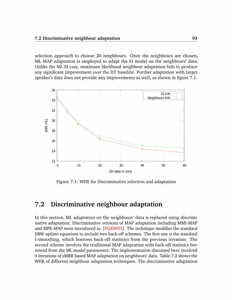
7.2 Discriminative neighbour adaptation 93

selection approach to choose 20 neighbours. Once the neighbours are chosen,ML MAP adaptation is employed to adapt the SI model on the neighbours’ data.Unlike the ML SI case, maximum likelihood neighbour adaptation fails to produceany significant improvement over the DT baseline. Further adaptation with targetspeaker’s data does not provide any improvements as well, as shown in figure 7.1.

22

24

26

28

30

32

34

36

0 10 20 30 40 50 60

WER

(%

)

SD data in mins


Figure 7.1: WER for Discriminative selection and adaptation

7.2 Discriminative neighbour adaptation

In this section, ML adaptation on the neighbours’ data is replaced using discrimi-native adaptation. Discriminative versions of MAP adaptation including MMI-MAPand MPE-MAP were introduced in [PGKW03]. The technique modifies the standardEBW update equations to include two back-off schemes. The first one is the standardI-smoothing, which borrows back-off statistics from the previous iteration. Thesecond scheme involves the traditional MAP adaptation with back-off statistics bor-rowed from the ML model parameters. The implementation discussed here involved4 iterations of sMBR based MAP adaptation on neighbours’ data. Table 7.2 shows theWER of different neighbour adaptation techniques. The discriminative adaptation


involving sMBR-MAP on neighbours’ data produced 8.5% relative improvementover baseline SI model.

Table 7.2: Discriminative neighbour adaptation.

SI training Neighbour adaptation WER (%)sMBR - 34.55sMBR ML MAP 34.49sMBR sMBR MAP 31.60

Further addition of target speaker adaptation continued to produce lower WERfor Neighbour-initialized model over the SI-initialized one, as shown in figure7.2. The improvements however is lower compared to ML case. Discriminativeadaptation can also be applied to the target speaker data, however, with a maximumof 1 hour of data sMBR-MAP did not produce significant improvement over theML-MAP hence the ML counterpart retained for this case.

22

24

26

28

30

32

34

36

0 10 20 30 40 50 60

WER

(%

)

SD data in mins



Table 7.3 shows the WER for different selection and adaptation setups. It canbe seen that there is almost no improvement by adapting the SI model on theneighbours data using ML-MAP criterion. Discriminative adaptation [PGKW03]

7.3 Discriminative neighbour selection 95

of the SI model on the neighbours data yielded a relative improvement of 8.5%compared to the unadapted model.

7.3 Discriminative neighbour selection

Discriminative criterion can also be used for neighbour selection in addition toadaptation. In this approach, the adaptation data of 5 mins is decoded using the SImodel to create lattices for the target speaker. Source speakers are chosen whosemodels maximize the average sMBR accuracy on the target speaker lattices. ThesMBR accuracy is calculated as

sMBR AccuracyT (S) =∑u∈UT

∑W∈W ′

γ(Ou,W |fT (λS))A(Wr,W ) (7.2)

where Wr is the reference transcription, W ′ are the competitor paths in thedenominator lattice, γ(Ou,W/λS) is the posterior of a lattice path according to the(adapted) source model fT (λS). A(Wr,W ) is the raw accuracy between the referenceand competitor state sequences. Analogous to likelihood and transformation basedneighbour selection, discriminative method leads to choosing neighbours who makeless error on the target speaker’s data.

Table 7.3: Discriminative selection and adaptation.

Selection Adaptation WER (%)- - 34.55 (SI)

ML transformation ML MAP 34.49ML transformation sMBR MAP 31.60

sMBR Acc. ML MAP 31.97sMBR Acc. sMBR MAP 31.00

From Table 7.3, it is interesting to note that neighbours selected using sMBRaccuracy produce 7.5% relative improvement over SI model, using ML MAP adap-tation. Comparing rows 2 and 3, it is noted that discriminative selection canlead to neighbours who produce less WER on target speaker data than ML basedselection. While the gains from discriminative selection and adaptation are notadditive, the combined technique still produces the best result of 10.3% relative


22

24

26

28

30

32

34

36

0 10 20 30 40 50 60

WER

(%

)

SD data in mins



improvement over the unadapted system. Figure 7.3 shows the WER of SI andneighbours-initialized systems with increasing target data.

7.4 Deep bottle-neck features

In this section, neighbour selection and adaptation is studied in the context ofa neural network based ASR system. The GMMs in the system are trained withfeatures from the bottle-neck layer of a multi-layered perceptron (MLP). The inputto the neural network are the same features the GMMs are trained with in the MFCCbased system, i.e MFCC followed by LDA and STC. These features are stacked witha window size of 5 and projected down to 150 dimensions using a second LDAmatrix. The second matrix helps with whitening the input features to the MLP inaddition to dimensionality reduction. This setup corresponds to the Type IV featuresinvestigated in [RPVC13].

The MLP has 4 hidden layers with dimensionality 465 and a bottle-neck layerof size 32. The architecture of the MLP is 150x465x465x465x32x465x1000 andit has a total of 1M parameters. The output layer has 1000 nodes representing

7.5 DBNF neighbour selection and adaptation 97

context-dependent states in the MFCC based system. The contextual decision treewith 3000 states is pruned down to 1000 leaves, which are used as targets for theMLP. However, the labels are obtained by force-aligning the utterances with the3000 state system similar to [SHRY13]. It has been shown that bottle-neck featuresperformed better with a lower number of targets than the original MFCC system[CCR+13]. Once the MLP is trained, the activations from the bottle-neck featuresare extracted, stacked with a window size of 9 and projected down to 32 dimensionswith a final LDA transform.

MLP is trained using backpropagation using the ’newbob’ learning rate schedule.The training starts with a learning rate of 0.008 until the accuracy on the held-outdata reduces and then it is divided in half for remaining epochs. The training stopsif there is no improvement of accuracy on the held-out set. The available trainingdata is subsampled to reduce the training time for the MLP. All the training speakersare retained, but they are restricted to a maximum of 15 mins to ensure there isample diversity in the MLP training data. 450 hours from 1691 speakers is used asa training set and 15 hour of data from 187 speakers is used as held-out set. Thetraining continued for 9 epochs with a batch size of 256. The final frame accuracyof the MLP on the training set is 46.3% and 43.0% on the held-out set.

7.5 DBNF neighbour selection and adaptation

The neighbour selection for DBNF system follows the transformation based tech-nique using ML criterion. The source speakers are ranked with the similarity scoreusing 5 mins of adaptation data. Top 20 neighbours are selected for each targetspeaker. Once the neighbours are chosen, MAP adaptation is performed on theneighbours data. Finally MLLR followed MAP adaptation is carried out on the targetspeaker’s data. Figure 7.4 shows the WER plots of neighbour-initialized and SIadapted systems for increasing target speaker’s data.

It is interesting to note that although DBNF system used ML based neighbourselection and adaptation, its performance is similar to MFCC system with discrimi-native adaptation. The additional MLP layers act as discriminatively trained modelsfor the ASR system.


22

24

26

28

30

32

34

36

0 10 20 30 40 50 60

WER

(%

)

SD data in mins


Figure 7.4: WER for DBNF neighbour selection and adaptation


The neighbour selection and adaptation techniques are studied for discriminativemodels in this chapter. A discriminative version of neighbour selection is introducedand compared with the DT adaptation. Their combination showed additionalimprovements. Finally, neighbour selection using DBNF features is studied andcompared against MFCC based systems.

Chapter 8

Text based neighbour selection

This chapter explores text-based neighbour selection techniques for improved speechrecognition. In the first set of experiments, text-based selection is used to augmentacoustic data selection. When not enough acoustic data is available, it is shown thattext based selection improves the reliability of neighbours selected for adaptation.In the second set of experiments, text based speaker selection is used to selectneighbours for language model adaptation. LM neighbours are analogous to acousticneighbours for a speaker, selected to reduce the perplexity of the target speaker onthe test set. Analysis on the neighbours selected based on domain and accent is alsopresented.

8.1 Textual features for neighbour selection

The previous chapters presented various neighbour selection and adaptation tech-niques using few mins of audio data from the target speaker. It is shown that asthe audio data available for the target speaker decreases, the quality of neighbourselected for adaptation of target SD models also decreases. In this section, textbased features are investigated to augment the acoustic data selection. There aremany applications where text data for a speaker is available in abundance, while it isdifficult to collect the audio data. For example, in the case of medical transcriptionif the doctor is starting with ASR for the first time, it is easy to access a list ofarchived reports while the corresponding audio data may not be available. Thereare also auxilliary text sources available in many applications to help improve theperformance of SD models. For example, in the case of desktop dictation, the users’

99

100 Chapter 8: Text based neighbour selection

emails may serve as representative text for the domain.

In this section, text-based features are used to select neighbours for adaptationof the SI model. In the acoustic neighbour selection, source speaker models areused to calculate likelihoods on the target speaker data. The speakers with thehighest likelihood are chosen as neighbours for adaptation. It was observed thatthe majority of selected neighbours belong to the same accent. However when theamount of adaptation data is varied, there was a deterioration in the quality ofneighbours selected. Table 6.2.2 showed WER of neighbour adapted system basedon the amount of target data available for selection. The goal of the followingexperiment is to compensate this lack of acoustic data using text-based features. Itexplores if additional text data can be used to augment acoustic neighbour selection.

A classifier is trained on the source speakers and their top 20 acoustic neighboursusing bag-of-word features. During testing, available text data for the test speakeris used to pre-select the neighbours for adaptation. The second round of selectionis carried out using the small amount of enrollment audio data. Since the secondround of selection is carried out on pre-selected source speakers, it produces betterneighbours compared to choosing neighbours considering the whole training data.


The same M*Modal medical transcription dataset is used here. For each of the 1876training speakers, neighbours are calculated by scanning through the entire trainingdataset. Choosing 20 neighbours was found to give the best acoustic adaptationperformance in the previous chapter. Hence the top 20 neighbours are used aspositive examples for the source speaker and 20 speakers with the lowest likelihoodscore as negative examples. A vocabulary of 20k words based on frequency is usedto calculate the bag of word features. The steps for preparing a training dataset fortext-based neighbour predictor is listed as follows.

• For each source speaker, calculate 20 speakers that produce the highest likeli-hood and 20 which produce the lowest likelihood.

• For each training example, 20k text features are extracted from the sourcespeaker’s reports based on unigram counts.

• It is appended with 20k text features extracted from the neighbour’s text data.

8.1 Textual features for neighbour selection 101

• The output class is based on whether the neighbour belong to the highest orlowest likelihood group.

Once the training examples are collected for all source speakers, a binary classi-fier is trained based solely on text features. In this experiment, 90% of the sourcespeakers (1690) formed the training set and remaining 10% is used as a devel-opment set. Linear SVM is used to train the text based neighbour predictor withthe help of LIBLINEAR [Lib] tool. The regularization constant is tuned usingthe development set. The classifier had an accuracy of 68% but the classificationperformance is not the main focus of this experiment. We are mainly interested inthe quality of neighbours selected for each test speaker. It is assumed we have 15reports for each speaker during training and test. In testing, the text data availablefor the test speaker and the source speaker is used to form the feature vector. Theoutput determines if the source speaker is a good neighbour for the test speaker.Once the neighbours are chosen, acoustic adaptation of the SI model is carried outusing the audio data from the neighbours.

8.1.2 Experiments

Table 8.1 shows the WER 20 neighbours selected randomly (5 trials) and using atext-based neighbour predictor. We can see that text-based neighbours provided 5%relative improvement over the baseline. One of the reasons the random selectionyield poor results is that the training dataset has less than 10% of South-Asianspeakers. Hence most of the random neighbours belong to the different accent. Inthe text-based selection, there are 40% South-Asian speakers on average, in the 20neighbours selected for adaptation. It is still less than nearly 70% of neighbours withmatched accent using acoustic data. Hence, there is only a moderate improvementwith text-based features. However, the text-based predictor can be used as a pre-selection criteria to augment acoustic selection in the case where there is only asmall amount of available target speech data.

Table 8.1: WER of neighbour selection using text-based selection.

Neighbour selection WER (%)- (SI) 45.73Random 50.12Text-based 43.20


The text-based predictor can be used as a first step to select matching accentneighbours for cases where enough speech data is not available for the targetspeaker. These neighbours can be rescored using the available audio data. In thisexperiment, the amount of target speech data available is varied from 1 to 5 mins.An initial set of 100 neighbours is chosen using the text-based selection and theyare rescored to choose 20 neighbours using acoustic neighbour selection as thesecond step. Table 8.2 shows the WER of acoustic and combined neighbour selectiontechniques. It can be seen that while reducing the amount of acoustic data from 5mins to 1 min caused 0.75% absolute reduction in WER, the text based pre-selectionreduced it to only 0.4%.

Table 8.2: WER of neighbour selection using audio and text-based selection.

Target speaker dataWER (%)

Acoustic data + Text data1.63 37.21 36.612.68 36.93 36.425.82 36.46 36.21

8.2 Language model adaptation

In the previous sections, we focussed our attention on adapting the acoustic modelto better model the target speaker. In this section, the neighbour selection andadaptation is carried out for the goal of language model adaptation. The languagemodel can be influenced by a variety of factors including dialect/accent of thedoctor, vocabulary choices based on geographical origin, hospital they work for,speciality of dictated content, etc. We use a different dataset with richer annotationsto allow us analyze these different factors influencing the language model. The newM*Modal dataset consists of 1350 speakers from 27 different specialties includingInternal medicine, Radiology, Pediatrics, etc. Each specialty contained 50 doctorsin the training set. Each doctor in the dataset is also annotated with the hospitalthey are from. The dataset contained 300K reports in total with 72M tokens and avocabulary of 58K words.

The LM neighbours are chosen as follows

• SI LM is trained using data from all source speakers.

8.3 Analysis 103

• For each source speaker, SD LM is trained using text data from the sourcespeaker.

• The 2 LMs are interpolated on the target speaker data, aka. transformationbased selection.

• The likelihood is then calculated on the target text data.

Once the neighbours are ranked based on the likelihood, the top N neighoursare chosen for adaptation. A neighbour LM is trained on their pooled data andinterpolated with the SI LM using the target speaker’s text data. We used the SI andSouth Asian adapted acoustic models to label speaker whether they are South-Asianor not based on the respective acoustic likelihood.

A test set of 15 speakers of South Asian accent with 50 reports each is used toanalyze the neighbour selection for LM adaptation. An additional 5 reports for eachspeaker is used for neighbour selection and adaptation. They are randomly selectedfrom different specialties to ensure there is no significant overlap. The followingsections analyze the influence of various dialectal factors such as accent, hospitalorigin and specialty in neighbour selection.

8.3 Analysis

In the first experiment, the influence of different factors in neighbour selection isanalyzed. Speciality of the doctor had the most significant influence on the LMneighours compared to the accent and the hospital labels (Mann-Whitney U test,p < 0.001). Figure 8.1 shows the neighbours at different ranks separated by thosefrom same domain as the target speaker and others. As the rank increases, the ratioof same domain neighbours increases. There is a cross-over between the two curvesat the end, as all the neighbours from the same domain have been selected and theremaining are out of domain ones. The graph clearly shows that the specialty of thetarget speaker has significant influence in neighbours selected for LM adaptation.

These documents are highly specific reports of patients, so it is obvious to seespeciality playing a larger role in the language model compared to accent labelsautomatically derived from acoustics. Comparing the experiments in section 8.1 and8.2, we can confirm that accent manifests itself in textual content in addition to thespeech data. We can automatically identify this influence using a classifier trainedsolely on the text, albeit with accents labels obtained using acoustic likelihoods. It


0

100

200

300

400

500

600

700

800

0 20 40 60 80 100

Cum

ulat

ive

Freq

.

Neighbours Rank

SpecialtyOthers

Figure 8.1: Rank of neighbours from same and different specialties

is helpful for choosing neighbours for acoustic model adaptation, particularly whenonly a small amount of target speech data is available. The neighbour selection andadaptation can be extended to LM adaptation where the technique automaticallypicks neighbours related to the speciality of the target speaker which has the highestinfluence on the content of the speech data.

8.4 ASR experiments

In this section, LM neighbour selection and adaptation is carried out for the testspeakers in original M*Modal test set. We start with determining the optimalnumber of neighbours for LM adaptation. Table 8.3 shows that perplexity of thetarget LM adapted using varying number of neighbours. The best result can beobtained using 30 neighbours.

In the next experiment, 30 neighbours are chosen for each test speaker and theirSD LMs are used in ASR decoding. Table 8.5 shows the WER of SI and neighbouradapted LMs on the South Asian test set. It is to be noted that the SI LM trained onthe new M*Modal dataset is used to obtain the baseline WER instead of internal

8.5 Summary and discussion 105

Table 8.3: Perplexity for varying neighbours in LM adaptation.

Rank Perplexity1 97.010 95.120 92.730 88.140 89.580 91.3100 93.7

medicine LM as in the previous experiments. Hence, the baseline WER is worse(47.7%) than reported before (45.73%). From the table, there is 11.5% relativereduction is perplexity which resulted in 6.7% relative reduction in WER.

Table 8.4: WER for neighbour selection based LM adaptation.

LM Perplexity WER (%)SI 83.9 47.8Neighbour adapt 74.2 44.6

Table 8.5 shows speaker WER for unadapted and neighbour adapted LMs. It canbe seen that the improvement is consistent across all speakers.


This chapter explored the use of text data for neighbour selection and adaptation.Text-based features can be shown to augment acoustic neighbour selection, whenthere is limited amount of speech data from the target speaker. The neighbourselection in the context of LM adaptation is discussed. The specialty of the targetspeaker is shown to influence LM neighbour selection through empirical analysis.The neighbour adapted LM produced 11.5% reduction in perplexity and 6.7%reduction in WER across 10 speakers.


Table 8.5: WER for LM adaptation using neighbour selection.

SpeakerWER (%)

SI-LM Neighbour Adaptation1 20.4 19.32 31.2 30.13 44.0 41.24 38.6 36.75 49.5 46.96 61.0 58.17 65.9 62.58 61.2 58.29 55.7 52.810 44.3 42.3Avg 47.8 44.6

Part V

Conclusion

107

Chapter 9

Summary and Future Directions

9.1 Thesis contributions

This thesis quantified the problems faced by accented speakers in 3 different ASR sce-narios and proposed novel research to address them. Techniques are introduced tohandle accented speakers in accent dependent systems, accent independent systemsand speaker dependent systems. The following list summarizes the contributions ineach ASR setup.

• Accent dependent systems: A decision tree based adaptation technique isproposed to specifically handle accent variations from source accent to thetarget, given the limited amount of adaptation data. Semi-continuous poly-phone decision tree specialization (SPDTS) is shown to efficiently use smallamount of adaptation data to adapt the baseline model to the target accent.The technique is evaluated on different datasets ranging from medium-scaleto large-scale tasks including WSJ, GALE and M*Modal medical dictation intwo languages. Compared to traditional MAP adaptation, SPDTS obtained arelative WER reduction of 4.2-13.6% on ML and discriminative baseline ASRmodels.

Bias sampling is proposed in the context of active and semi-supervised learningto leverage unlabeled target accent data in a large corpus. Active learningtechnique resulted in a reduction of labelling cost by 50% and semi-supervisedlearning provided additional improvement of 2-15.9% relative WER oversupervised baseline.

109

110 Chapter 9: Summary and Future Directions

• Accent independent systems: Decision tree based accent robustness analysis isintroduced to measure the accent normalization characteristics of differentfront-ends. Traditional 4-layer bottle-neck MLP is shown to normalize for gen-der, but are still sensitive to accent variations. Deeper architectures and deeperbottle-neck layers are shown to have better normalization characteristics whencompared to MFCC or MLP.

Accent-aware training is proposed to augment accent labels to spectral featuresduring training of BN front-ends. It is shown that labelling a subset of speakerswith accents (150 hours) and using them as additional features in accent-aware training results in a WER of 33.78% which is better than 34.75% WERobtained by training an accent agnostic model on a much larger dataset (450hours).

• Speaker dependent systems: The problems faced by accented speakers in thecontext of speaker dependent models are highlighted. Neighbour selectionand adaptation techniques are proposed to create target speaker-dependentASR model using few mins of adaptation data. These technique produce animprovement of 31.2% relative over SI+MLLR baseline. The neighbours arefurther analyzed to show that accent plays a crucial role in the neighbours cho-sen automatically for the target speaker. The neighbour selection is extensivelyanalyzed in different experiments including varying the number of neighbours,amount of adaptation data and supervised Vs unsupervised adaptation.

A discriminative version of the neighbour selection using sMBR is formulatedand shown to provide gains of around 10.1% relative over ML neighbourselection. Text-based neighbour selection is explored in the case of lack ofsufficient or no audio data from the target speaker and shown to provideconsistent gains of around 1-2% over audio-only neighbour selection. Thetechnique is ported to LM adaptation and the neighbour selection is analyzedalong different factors such as accent, speciality of the dictation content andplace of work. LM adaptation resulted in 11.5% reduction in perplexity and6.7% relative reduction in WER compared to the unadapted LM.

9.2 Future Directions

This work can have several future directions. Some of them are listed below

• Dialect modeling using RNNLM: The current experiments mainly use Ngram

9.2 Future Directions 111

models for language model adaptation. It will be interesting to think aboutlanguage model adaptation and interpolation in the context of RNN architec-ture.

• The thesis has explored on acoustic and language model adaptation in thecontext of accented speakers. Other models in the ASR such as vocabularycan be adapted based on the dialect of the user.

• The accent dependent chapter introduced decision tree based accent adapta-tion to model contextual rules in the target accent. This technique is comple-mentary to pronunciation modeling whose aim is to change the surface formsin the dictionary using re-write rules. It will be interesting to compare theinterplay between these two modules and investigate tighter integration ofboth techniques.

Bibliography

[Bac13] Michiel Bacchiani. Rapid adaptation for mobile speech applications.In ICASSP, 2013. 74

[BBS+08] Michiel Bacchiani, Francoise Beaufays, Johan Schalkwyk, Mike Schus-ter, and Brian Strope. Deploying goog-411: Early lessons in data,measurement, and testing. In ICASSP, pages 5260–5263, 2008. 3

[BBS09] Steffen Bickel, Michael Bruckner, and Tobias Scheffer. Discriminativelearning under covariate shift. Journal of Machine Learning Research,10, 2009. 27, 40

[BHC10] Fadi Biadsy, Julia Hirschberg, and Michael Collins. Dialect recognitionusing a phone-gmm-supervector-based svm kernel. In INTERSPEECH,pages 753–756, 2010. 57

[BI10] John Blitzer and Hal Daume III. ICML tutorial on domain adaptation.http://adaptationtutorial.blitzer.com, June 2010. 27, 40

[BK03] Christophe Van Bael and Simon King. An accent-independent lexiconfor automatic speech recognition. In ICPhS, pages 1165–1168, 2003.4, 12

[BMJ12] Fadi Biadsy, Pedro Moreno, and Martin Jansche. Google’s cross-dialectarabic voice search. In ICASSP, 2012. 3

[BVS10] Francoise Beaufays, Vincent Vanhoucke, and Brian Strope. Unsuper-vised discovery and training of maximally dissimilar cluster models. InINTERSPEECH, pages 66–69, 2010. 74

[CCR+13] Jia Cui, Xiaodong Cui, Bhuvana Ramabhadran, Janice Kim, BrianKingsbury, Jonathan Mamou, Lidia Mangu, Michael Picheny, Tara N.

113

http://adaptationtutorial.blitzer.com

114 Bibliography

Sainath, and Abhinav Sethy. Developing speech recognition systemsfor corpus indexing under the iarpa babel program. In ICASSP, 2013.97

[Che01] Rathinavelu Chengalvarayan. Accent-independent universal hmm-based speech recognizer for american, australian and british english.In INTERSPEECH, pages 2733–2736, 2001. 50

[CJ06] Constance Clarke and Daniel Jurafsky. Limitations of mllr adaptationwith spanish-accented english: an error analysis. In INTERSPEECH,2006. 5, 18

[CLWL00] Kuan-Ting Chen, Wen-Wei Liau, Hsin-Min Wang, and Lin-Shan Lee.Fast speaker adaptation using eigenspace-based maximum likelihoodlinear regression. In INTERSPEECH, pages 742–745, 2000. 74

[CMN09] Monica Caballero, Asuncion Moreno, and Albino Nogueiras. Multi-dialectal spanish acoustic modeling for speech recognition. SpeechCommunication, 51(3):217–229, 2009. 5, 50

[CMRR08] Corinna Cortes, Mehryar Mohri, Michael Riley, and Afshin Ros-tamizadeh. Sample selection bias correction theory. In ALT, pages38–53, 2008. 27, 40

[Com01] Dirk Van Compernolle. Recognizing speech of goats, wolves, sheepand ... non-natives. Speech Communication, 35(1-2):71–79, 2001. 3

[DDNK97] V. Digalakis, V. Digalakis, L. Neumeyer, and J. Kaja. Developmentof dialect-specific speech recognizers using adaptation methods. InICASSP, pages 1455–1458, 1997. 5

[Den11] Li Deng. Front-end, back-end, and hybrid techniques for noise-robustspeech recognition. In Robust Speech Recognition of Uncertain or MissingData, pages 67–99. 2011. 50

[FSGL11] Thiago Fraga-Silva, Jean-Luc Gauvain, and Lori Lamel. Lattice-basedunsupervised acoustic model training. In ICASSP, pages 4656–4659,2011. 39

[Fur89] Sadaoki Furui. Unsupervised speaker adaptation method based onhierarchical spectral clustering. In ICASSP, 1989. 74

115

[FWK08] Joe Frankel, Dong Wang, and Simon King. Growing bottleneck featuresfor tandem asr. In INTERSPEECH, page 1549, 2008. 54

[GAAD+05] Jean-Luc Gauvain, Gilles Adda, Martine Adda-Decker, Alexandre Al-lauzen, Veronique Gendner, Lori Lamel, and Holger Schwenk. Whereare we in transcribing french broadcast news? In INTERSPEECH, pages1665–1668, 2005. 3

[Gal96] M. J. F. Gales. The generation and use of regression class trees forMLLR adaptation. Technical report, Cambridge University, 1996. 78

[Gal98] M. J. F. Gales. Maximum likelihood linear transformations for HMM-based speech recognition. Computer Speech & Language, 12(2):75–98,1998. 70, 72

[Gal00] Mark J. F. Gales. Cluster adaptive training of hidden markov models.IEEE Transactions on Speech and Audio Processing, 8(4):417–428, 2000.75

[Gal01] M. J. F. Gales. Multiple-cluster adaptive training schemes. In ICASSP,2001. 75

[Gal11a] M. J. F. Gales. Model-based approaches to handling uncertainty. InRobust Speech Recognition of Uncertain or Missing Data, pages 101–125.2011. 50

[Gal11b] M. J. F. Gales. Model-based approaches to handling uncertainty. InRobust Speech Recognition of Uncertain or Missing Data, pages 101–125.2011. 50

[GF08] Frantisek Grezl and Petr Fousek. Optimizing bottle-neck features forlvcsr. In ICASSP, pages 4729–4732, 2008. 54

[GH06] Matthew Gibson and Thomas Hain. Hypothesis spaces for minimumbayes risk training in large vocabulary speech recognition. In INTER-SPEECH, 2006. 91

[GKKC07] Frantisek Grezl, Martin Karafiat, Stanislav Kontar, and Jan Cernocky.Probabilistic and bottle-neck features for lvcsr of meetings. In ICASSP,volume 4, pages IV–757 –IV–760, april 2007. 55

116 Bibliography

[GL94a] Jean-Luc Gauvain and Chin-Hui Lee. Maximum a posteriori estimationfor multivariate gaussian mixture observations of markov chains. IEEETransactions on Speech and Audio Processing, 2(2):291–298, 1994. 5,40

[GL94b] Jean-Luc Gauvain and Chin-Hui Lee. Maximum a posteriori estimationfor multivariate gaussian mixture observations of markov chains. IEEETransactions on Speech and Audio Processing, 2(2):291–298, 1994. 72

[GRK04] Silke Goronzy, Stefan Rapp, and Ralf Kompe. Generating non-nativepronunciation variants for lexicon adaptation. Speech Communication,42(1):109–123, 2004. 12

[HAH01] Xuedong Huang, Alex Acero, and Hsiao-Wuen Hon. In Spoken LanguageProcessing: A Guide to Theory, Algorithm and System Development.Prentice Hall, 2001. 18

[HCC01] Chao Huang, Eric Chang, and Tao Chen. Accent issues in large vocabu-lary continuous speech recognition. Technical Report MSR-TR-2001-69,Microsoft Research, 2001. 3

[HCC02] Chao Huang, Tao Chen, and Eric Chang. Speaker selection trainingfor large vocabulary continuous speech recognition. In ICASSP, pages609–612, 2002. 75, 76

[HDY+12] Geoffrey Hinton, Li Deng, Dong Yu, George Dahl, Abdel rahman Mo-hamed, Navdeep Jaitly, Andrew Senior, Vincent Vanhoucke, PatrickNguyen, Tara Sainath, and Brian Kingsbury. Deep neural networks foracoustic modeling in speech recognition. Signal Processing Magazine,2012. 61

[HFT+09] Roger Hsiao, Mark Fuhs, Yik-Cheung Tam, Qin Jin, Ian Lane, and TanjaSchultz. The cmu-interact mandarin transcription system for gale. InGALE Book, 2009. 3

[HJ91] Hynek Hermansky and Louis Anthony Cox Jr. Perceptual linear pre-dictive (plp) analysis-resynthesis technique. In EUROSPEECH, 1991.49

[HJZ10] Sheng-Jun Huang, Rong Jin, and Zhi-Hua Zhou. Active learning byquerying informative and representative examples. In NIPS, pages892–900, 2010. 26

117

[HM94] Hynek Hermansky and Nelson Morgan. Rasta processing of speech.IEEE Transactions on Speech and Audio Processing, 2(4):578–589, 1994.49

[HP99] Jing Huang and Mukund Padmanabhan. A study of adaptation tech-niques on a voicemail transcription task. In EUROSPEECH, 1999. 75

[HTRG02] Dilek Z. Hakkani-Tur, Giuseppe Riccardi, and Allen L. Gorin. Activelearning for automatic speech recognition. In ICASSP, pages 3904–3907, 2002. 26

[Hum97] J.J. Humphries. Accent modelling and adaptation in auto-matic speech recognition. http://svr-www.eng.cam.ac.uk/~jjh11/publications/PhD_thesis.ps.gz, 1997. 5, 12

[HW97] J. J. Humphries and Philip C. Woodland. Using accent-specific pronun-ciation modelling for improved large vocabulary continuous speechrecognition. In EUROSPEECH, 1997. 3, 4, 12

[IMS+04] Shajith Ikbal, Hemant Misra, Sunil Sivadas, Hynek Hermansky, andHerve Bourlard. Entropy based combination of tandem representationsfor noise robust asr. In INTERSPEECH, 2004. 49

[ISJ+12] N. Itoh, T.N. Sainath, D.N. Jiang, J. Zhou, and B. Ramabhadran. N-bestentropy based data selection for acoustic modeling. In ICASSP, pages4133–4136, 2012. 25, 26, 27, 30

[KG09] D. K. Kim and M. J. F. Gales. Adaptive training with noisy constrainedmaximum likelihood linear regression for noise robust speech recogni-tion. In INTERSPEECH, pages 2383–2386, 2009. 50

[KMN12] Herman Kamper, Felicien Jeje Muamba Mukanya, and Thomas Niesler.Multi-accent acoustic modelling of south african english. Speech Com-munication, 54(6):801–813, 2012. 5, 50

[KNJ+98] Roland Kuhn, Patrick Nguyen, Jean-Claude Junqua, Lloyd Goldwasser,Nancy Niedzielski, Steven Fincke, Ken Field, and Matteo Contolini.Eigenvoices for speaker adaptation. In ICSLP, 1998. 73

[KW99] Thomas Kemp and Alex Waibel. Unsupervised training of a speechrecognizer: recent experiments. In EUROSPEECH, 1999. 37

http://svr-www.eng.cam.ac.uk/~jjh11/publications/PhD_thesis.ps.gz

http://svr-www.eng.cam.ac.uk/~jjh11/publications/PhD_thesis.ps.gz

118 Bibliography

[LG] Karen Livescu and James Glass. Lexical modeling of non-native speechfor automatic speech recognition. In ICASSP, pages 1683 – 1686. 4

[LGN09] Jonas Loof, Christian Gollan, and Hermann Ney. Cross-language boot-strapping for unsupervised acoustic model training: rapid developmentof a polish speech recognition system. In INTERSPEECH, pages 88–91,2009. 37

[Lib] Phoneme. http://www.csie.ntu.edu.tw/~cjlin/liblinear/. 101

[Liv99] K. Livescu. Analysis and modeling of non-native speech for au-tomatic speech recognition. http://www.sls.lcs.mit.edu/sls/

publications/1999/msthesis-livescu.pdf, 1999. 12

[LW94] C. J. Leggetter and Philip C. Woodland. Speaker adaptation of con-tinuous density HMMs using multivariate linear regression. In ICSLP,1994. 72

[LW95] C.J. Leggetter and P.C. Woodland. Maximum likelihood linear re-gression for speaker adaptation of continuous density hidden markovmodels. Computer Speech & Language, 9(2):171–185, 1995. 5

[MBS00] Lidia Mangu, Eric Brill, and Andreas Stolcke. Finding consensus inspeech recognition: word error minimization and other applications ofconfusion networks. Computer Speech & Language, 14(4), 2000. 27,39, 42

[MGA+06] Spyridon Matsoukas, Jean-Luc Gauvain, Gilles Adda, ThomasColthurst, Chia-Lin Kao, Owen Kimball, Lori Lamel, Fabrice Lefevre,Jeff Z. Ma, John Makhoul, Long Nguyen, Rohit Prasad, Richard M.Schwartz, Holger Schwenk, and Bing Xiang. Advances in transcriptionof broadcast news and conversational telephone speech within thecombined ears bbn/limsi system. IEEE Transactions on Audio, Speech &Language Processing, 14(5):1541–1556, 2006. 3

[MH07] Brian Kan-Wing Mak and Roger Wend-Huu Hsiao. Kernel eigenspace-based mllr adaptation. IEEE Transactions on Audio, Speech & LanguageProcessing, 15(3):784–795, 2007. 73

[MHJ+10] Florian Metze, Roger Hsiao, Qin Jin, Udhyakumar Nallasamy, andTanja Schultz. The 2010 cmu gale speech-to-text system. In INTER-SPEECH, pages 1501–1504, 2010. 16, 32

http://www.csie.ntu.edu.tw/~cjlin/liblinear/

http://www.sls.lcs.mit.edu/sls/publications/1999/msthesis-livescu.pdf

http://www.sls.lcs.mit.edu/sls/publications/1999/msthesis-livescu.pdf

119

[MHu] Accents research. http://www.phon.ucl.ac.uk/home/mark/accent.4

[ML10] Robert C. Moore and William Lewis. Intelligent selection of languagemodel training data. In ACL (Short Papers), pages 220–224, 2010. 29

[MS08] Jeff Z. Ma and Richard M. Schwartz. Unsupervised versus supervisedtraining of acoustic models. In INTERSPEECH, pages 2374–2377, 2008.37

[MW47] H. B. Mann and D. R. Whitney. On a test of whether one of two randomvariables is stochastically larger than the other. Annals of MathematicalStatistics, 18(1):50–60, 1947. 84

[NFW+13] Udhyakumar Nallasamy, Mark Fuhs, Monika Woszczyna, Florian Metze,and Tanja Schultz. Neighbour selection and adaptation for rapidspeaker-dependent asr. In ASRU, 2013. 6

[NGM+11] Udhyakumar Nallasamy, Michael Garbus, Florian Metze, Qin Jin,Thomas Schaaf, and Tanja Schultz. Analysis of dialectal influencein pan-arabic asr. In INTERSPEECH, pages 1721–1724, 2011. 4, 6, 12

[NMS11] Udhyakumar Nallasamy, Florian Metze, and Thomas Schaaf. Nor-malization of gender, dialect and speaking style using probabilisticfront-ends. In DAGA, 2011. 6

[NMS12a] Udhyakumar Nallasamy, Florian Metze, and Tanja Schultz. Activelearning for accent adaptation in automatic speech recognition. In SLT,2012. 6

[NMS12b] Udhyakumar Nallasamy, Florian Metze, and Tanja Schultz. Enhancedpolyphone decision tree adaptation for accented speech recognition.In Interspeech, 2012. 3, 6, 32, 40

[NMS12c] Udhyakumar Nallasamy, Florian Metze, and Tanja Schultz. Semi-supervised learning for speech recognition in the context of accentadaptation. In MLSLP Symposium, 2012. 6, 29

[NSK11] Scott Novotney, Richard M. Schwartz, and Sanjeev Khudanpur. Unsu-pervised arabic dialect adaptation with self-training. In INTERSPEECH,pages 541–544, 2011. 5, 37

http://www.phon.ucl.ac.uk/home/mark/accent

120 Bibliography

[NWJ99] Patrick Nguyen, Christian Wellekens, and Jean-Claude Junqua. Maxi-mum likelihood eigenspace and mllr for speech recognition in noisyenvironments. In EUROSPEECH, 1999. 73

[PBNP98] Mukund Padmanabhan, Lalit R. Bahl, David Nahamoo, and Michael A.Picheny. Speaker clustering and transformation for speaker adaptationin speech recognition systems. IEEE Transactions on Speech and AudioProcessing, 6(1):71–77, 1998. 75

[PGKW03] Daniel Povey, M. J. F. Gales, Do Yeong Kim, and Philip C. Woodland.MMI-MAP and MPE-MAP for acoustic model adaptation. In INTER-SPEECH, 2003. 93, 94

[PW02] Daniel Povey and Philip C. Woodland. Minimum phone error andi-smoothing for improved discriminative training. In ICASSP, pages105–108, 2002. 91

[PY12a] Daniel Povey and Kaisheng Yao. A basis representation of constrainedmllr transforms for robust adaptation. Computer Speech & Language,26(1):35–51, 2012. 41

[PY12b] Daniel Povey and Kaisheng Yao. A basis representation of constrainedmllr transforms for robust adaptation. Computer Speech & Language,26(1):35–51, 2012. 74

[Qui] Quicknet toolkit. http://www1.icsi.berkeley.edu/Speech/qn.html.54

[Ram05] Bhuvana Ramabhadran. Exploiting large quantities of spontaneousspeech for unsupervised training of acoustic models. In INTERSPEECH,pages 1617–1620, 2005. 37

[RBF+99] Michael Riley, William Byrne, Michael Finke, Sanjeev Khudanpur, An-drej Ljolje, John W. McDonough, Harriet J. Nock, Murat Saraclar,Charles Wooters, and George Zavaliagkos. Stochastic pronunciationmodelling from hand-labelled phonetic corpora. Speech Communica-tion, 29(2-4):209–224, 1999. 5

[RBGP12] K. Reidhammer, T. Bocklet, A. Ghoshal, and D. Povey. Revisitingsemi-continuous hidden markov models. In ICASSP, 2012. 14

http://www1.icsi.berkeley.edu/Speech/qn.html

121

[RHT05] Giuseppe Riccardi and Dilek Hakkani-Tur. Active learning: theory andapplications to automatic speech recognition. IEEE Transactions onSpeech and Audio Processing, 13(4):504–511, 2005. 25

[RPVC13] Shakti Rath, Daniel Povey, Karel Vesely, and Jan Cernocky. Improvedfeature processing for deep neural networks. In ICASSP, 2013. 96

[SA11] Michael L. Seltzer and Alex Acero. Factored adaptation for separablecompensation of speaker and environmental variability. In ASRU, pages146–151, 2011. 50

[SBD95] Ananth Sankar, Francoise Beaufays, and Vassilios Digalakis. Trainingdata clustering for improved speech recognition. In EUROSPEECH,1995. 74

[Set09] Burr Settles. Active learning literature survey. Computer SciencesTechnical Report 1648, University of Wisconsin–Madison, 2009. 25

[SHRY13] Andrew Senior, Georg Heigold, Marc’aurelio Ranzato, and Ke Yang. Anempirical study of learning rates in deep neural networks for speechrecognition. In ICASSP, 2013. 97

[SK11] Peter Smit and Mikko Kurimo. Using stacked transformations forrecognizing foreign accented speech. In ICASSP, pages 5008–5011,2011. 5, 12, 50

[SMB11] Hagen Soltau, Lidia Mangu, and Fadi Biadsy. From modern standardarabic to levantine asr: Leveraging gale for dialects. In ASRU, pages266–271, 2011. 3, 5, 17, 46

[SRN+12] Tara N. Sainath, Bhuvana Ramabhadran, David Nahamoo, DimitriKanevsky, Dirk Van Compernolle, Kris Demuynck, Jort F. Gemmeke,Jerome R. Bellegarda, and Shiva Sundaram. Exemplar-based process-ing for speech recognition: An overview. IEEE Signal Process. Mag.,29(6):98–113, 2012. 75

[SSK+09] Hagen Soltau, George Saon, Brian Kingsbury, Hong-Kwang Jeff Kuo,Lidia Mangu, Daniel Povey, and Ahmad Emami. Advances in arabicspeech transcription at ibm under the darpa gale program. IEEETransactions on Audio, Speech & Language Processing, 17(5):884–894,2009. 3, 14

122 Bibliography

[Stu08] Sebastian Stuker. Modified polyphone decision tree specialization forporting multilingual grapheme based asr systems to new languages.In ICASSP, pages 4249–4252, 2008. 12

[SW00] T. Schultz and A. Waibel. Polyphone decision tree specialization forlanguage adaptation. In ICASSP, 2000. 12, 13, 18

[THTS05] Gokhan Tur, Dilek Z. Hakkani-Tur, and Robert E. Schapire. Combiningactive and semi-supervised learning for spoken language understand-ing. Speech Communication, 45(2):171–186, 2005. 25

[TO09] Katrin Tomanek and Fredrik Olsson. A web survey on the use of activelearning to support annotation of text data. In Workshop on ActiveLearning for NLP, HLT ’09, pages 45–48, Stroudsburg, PA, USA, 2009.25

[Tom00] Laura Mayfield Tomokiyo. Lexical and acoustic modeling of non-nativespeech in lvscr. In INTERSPEECH, pages 346–349, 2000. 4, 5, 12

[Uni] Unisyn lexicon. http://www.cstr.ed.ac.uk/projects/unisyn. 4, 12

[VLG10] Dimitra Vergyri, Lori Lamel, and Jean-Luc Gauvain. Automatic speechrecognition of multiple accented english data. In INTERSPEECH, pages1652–1655, 2010. 5, 12

[VOWY97] V. Valtchev, J. J. Odell, Philip C. Woodland, and Steve J. Young. Mmietraining of large vocabulary recognition systems. Speech Communica-tion, 22(4):303–314, 1997. 91

[VRF10] Ravichander Vipperla, Steve Renals, and Joe Frankel. Augmentationof adaptation data. In INTERSPEECH, pages 530–533, 2010. 75, 76

[WC01] Jian Wu and Eric Chang. Cohorts based custom models for rapidspeaker and dialect adaptation. In INTERSPEECH, pages 1261–1264,2001. 75, 76

[Wel82] J.C. Wells. Accents of English:. Accents of English. Cambridge UniversityPress, 1982. 4

[WN05] Frank Wessel and Hermann Ney. Unsupervised training of acousticmodels for large vocabulary continuous speech recognition. IEEETransactions on Speech and Audio Processing, 13(1):23–31, 2005. 37

http://www.cstr.ed.ac.uk/projects/unisyn

123

[WS03] Zhirong Wang and Tanja Schultz. Non-native spontaneous speechrecognition through polyphone decision tree specialization. In INTER-SPEECH, 2003. 5, 13

[YBM+01] Shinichi Yoshizawa, Akira Baba, Kanako Matsunami, Yuichiro Mera,Miichi Yamada, Akinobu Lee, and Kiyohiro Shikano. Evaluation onunsupervised speaker adaptation based on sufficient hmm statictics ofselected speakers. In INTERSPEECH, pages 1219–1222, 2001. 76

[YG06] Kai Yu and M. J. F. Gales. Discriminative cluster adaptive training.IEEE Transactions on Audio, Speech & Language Processing, 14(5):1694–1703, 2006. 75

[YGWW10] Kai Yu, Mark J. F. Gales, Lan Wang, and Philip C. Woodland. Unsuper-vised training and directed manual transcription for LVCSR. SpeechCommunication, 52(7-8):652–663, 2010. 25, 37

[YVDA10] Dong Yu, Balakrishnan Varadarajan, Li Deng, and Alex Acero. Ac-tive learning and semi-supervised learning for speech recognition: Aunified framework using the global entropy reduction maximizationcriterion. Computer Speech & Language, 24(3), 2010. 25, 26, 27, 39

[ZBB+12] Heiga Zen, Norbert Braunschweiler, Sabine Buchholz, Mark J. F. Gales,Kate Knill, Sacha Krstulovic, and Javier Latorre. Statistical parametricspeech synthesis based on speaker and language factorization. IEEETransactions on Audio, Speech & Language Processing, 20(6):1713–1724,2012. 6

[ZW97] Puming Zhan and Alex Waibel. Vocal tract length normalization forlarge vocabulary continuous speech recognition. Technical report,Carnegie Mellon University, 1997. 69, 83

Adaptation techniques to improve ASR performance on ...

Documents

Transcript of Adaptation techniques to improve ASR performance on ...