AD-All 774 MASSACHUSETTS INST OF TECH CAMBRIDGE AEROPHYSICS LAB F/B 20/1DEVELOPMENT OF AN AIRBORNE SONIC THERMOMETER(U)FO9A28-8B-K-OBB9

UNCLASSIFIED AFGL-TR-82-017q NL

IILIlIIIIIIIIlIIIIIIIIIIhhIlIIIlffIIII lfllfIIIfEEIEEEEIIIIEII

llllllIlllEllE

iib

UnclassifiedSECURITY CLASSIFICATION OF THIS PAGE (Winm Doat ntered)

REPORT DOCUMENTATION PAGE BEFORE CMPL oN1. REPORT NUMBER 2. GOVT ACCESSION NO. 3. RECIPIENT'S CATALOG NUMBER

AFGL-TR-82-0179 P I%4 4. TITLE (md Subtitle) S. TYPE OF REPORT A PERIOD COVERED

, Final ReportDevelopment of an Airborne Sonic Thermometer Inal Report1 July 1980 - 30 Sept. 1982

6. PERFORMING ORG. REPORT NUMBER

7. AUTHOR(*) 6. CONTRACT OR GRANT NUMBER(s)

Tore R. Christiansen F19628-80-K-0089

9. PERFORMING ORGANIZATION NAME AND ADDRESS 10. PROGRAM ELEMENT. PROJECT, TASICAREA & WORK UNIT NUMBERS

Aerophysics LaboratoryMassachusetts Institute of Technology 2310G3 AV

Cambridge, Massachusetts 02139

It. CONTROLLING OFFICE NAME AND ADDRESS 12. REPORT DATE

Air Force Geophysics Laboratory September 1982Hanscom AFB, MA 01731 13. NUMBER OF PAGESMonitor/Edmund A. Murphy/LKD 124

14. MONITORING AGENCY NAME A ADDRESS(if dflferent from Controlling Office) IS. SECURITY CLASS. (of this report)

Unclassified

1S.. DECLASSIFICATION/OOWNGRADING.SCHEDULE

IS. DISTRIBUTION STATEMENT (of this Report)

Approved for public release; distribution unlimited

I?. DISTRIBUTION STATEMENT (of the abstract entered In Block 20, It different from Report)

18. SUPPLEMENTARY NOTES

It. KEY WORDS (Continue on reverse side If necessary and Identify by block number)

Acoustic thermometerSound speed measurementTroposphere/stratosphereTemperature fluctuation

SO. ABSTRACT (Continue on rever" side It neoeesary and Identify by block number)

An airborne sonic thermometer has been developed asid is now ready for

flight testing. The designed instrument uses a specially developed electro-

magnetic transmitter, a sensitive condenser microphone and integrated circuit

components.The air temperature is determined by measuring the phase difference betwmen

the transmitted and received signals across an acoustic path in the medium.

The phase information is delivered as a changing dc-level voltage, as a digital

DD I OM 1473 EITION OF I NOV 65 IS OBSOLETE UnclassifiedSECURITY CLASSIFICATI' 0 THIS PAGE (linen Data EtoMee)

SECUIUYv CLASSFICATION OF THIS PAGS(Whaf ONG. Eabecrd

Block 20. cont'd.signal and in the form of two phase shifted squarevaves.

Improvements of the present design are needed to exclude the effect ofwind speed on the temperature measurement and in the accuracy of the calibration

of the signal outputs. Onice these are included. howvewr, temperature measure-ments to an accuracy of plus minus one tenth of a degree centigrade, over atemperature range from plus 250 C to minus WOC, should be available.

Uniclassi fied

SeCUo"Vt CtASSIPICAIO4 dip THIS PA*36Umbs Do*. antend)

-3-

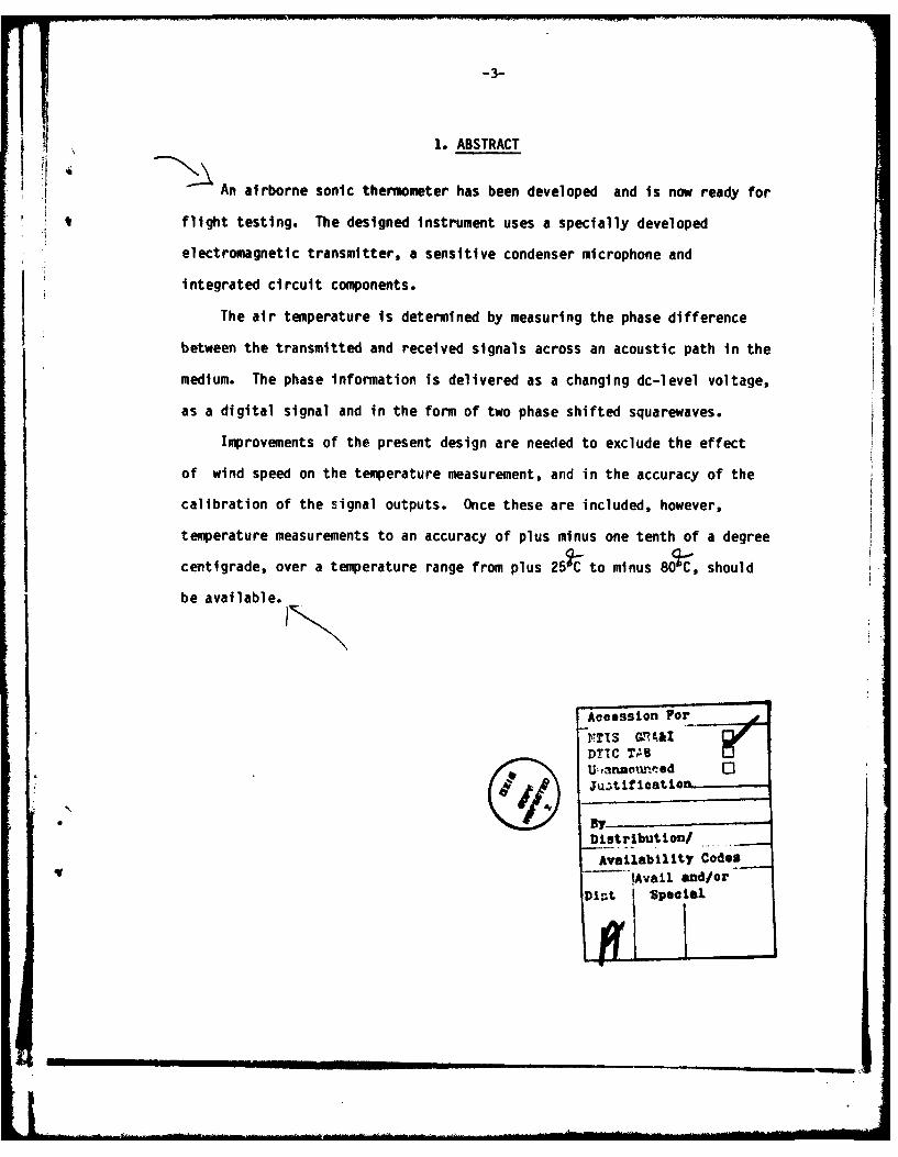
1. ABSTRACT

An airborne sonic thermometer has been developed and is now ready for

t flight testing. The designed instrument uses a specially developed

electromagnetic transmitter, a sensitive condenser microphone and

integrated circuit components.

The air temperature is determined by measuring the phase difference

between the transmitted and received signals across an acoustic path in the

medium. The phase information is delivered as a changing dc-level voltage,

as a digital signal and in the form of two phase shifted squarewaves.

Improvements of the present design are needed to exclude the effect

of wind speed on the temperature measurement, and in the accuracy of the

calibration of the signal outputs. Once these are included, however,

temperature measurements to an accuracy of plus minus one tenth of a degree

centigrade, over a temperature range from plus 25Cto minus 80bC, should

be available.

AcoessiOn For

TITS CG'AhIDTTC TABUt anaowned 01JuztiAicatlon

• ByDlstribution/Availability Codes

Avail and/or

Dict SPGO lal

T I

2. CONTENTS

1. SUMMARY 32. CONTENTS 5

-with list of Appendicies and Figures

3. INTRODUCTION 9

- outlines the reasons for, and scope of the project

4. ACOUSTIC FLOW MEASUREMENT TECHNIQUES 11

- an explanation of the principles of sonic thermometry and anemometry

5. SONIC THERMOMETRY IN THE ATMOSPHERE 20

- some problems of measureing in the atmosphere, and a theoretical

estimate of the possible ranges of measurement

6. THE BALLOONBORNE ACOUSTIC THERMOMETER (BAT) 25

- a description of the final instrument as delivered for flight

testing

The electronic components

The acoustic components

The casing and insulation

7. TEMPERATURE MEASUREMENT 51

- gives calibration curves, together with the expected sensitivity

in atmospheric temperature measurements

8. METEOROLOGICAL SIGNIFICANCE 63

6 - reasons for measuring temperature sonically rather than by

other means.

9. CONCLUSIONS AND RECOMMENDATIONS 66

-final words with possible future improvements

- ,- -

10. ACKNOWILEDGEMENTS 69

11. REFERENCES 71

APPENDIC JES 75

LIST OF FIGURES AND TABLES

1. Sound ray vectors showing the principle of sonic velocity 15

measurement

2. Temperature ranges for different choices of length of acoustic path 23

3. Block diagram of the Balloonborne Sonic Thermometer (BAT) 27

4. Component side of the electronic circuit boards 36

5. Reverse side of the electronic circuit boards 37

6. The electromagnetic transmitter and condenser microphone 43

7. The arm for holding the acoustic components 48

8. Exterior view of the flight instrument 49

9. Interior view of the flight instrument 50

10. The expected sensitivity of the phase comparator output 51

11. The expected sensitivity of the digital phase meter output 51

12. The expected behaviour of the final design 52

13. The one-dimensional theoretical response of the dc-telemetry 56

signal

14. The set up for calibration at AFGL 59

15. The results of calibration with theoretical predictions 61

... ..

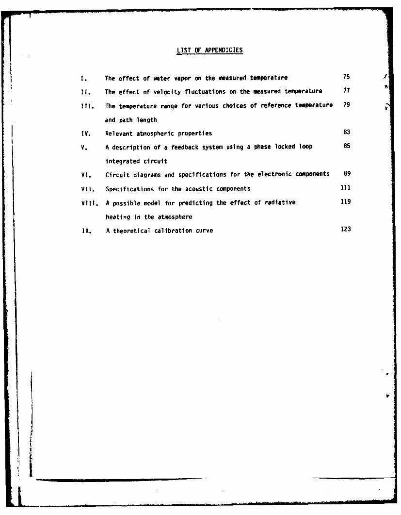
LIST OF APPENDICIES

I. The effect of water vapor on the measured temperature 75

II. The effect of velocity fluctuations on the measured temperature 77

III. The temperature range for various choices of reference temperature 79 I

and path length

IV. Relevant atmospheric properties 83

V. A description of a feedback system using a phase locked loop 85

integrated circuit

VI. Circuit diagrams and specifications for the electronic components 89

VII. Specifications for the acoustic components ill

VIII. A possible model for predicting the effect of radiative 119

heating in the atmosphere

IX. A theoretical calibration curve 123

,~ I.

-9-

3. INTRODUCTION

In order to study in m~ore detail the thermal composition and the

turbulence structure of the atmosphere, more accurate and time responsive

thermometers would be of great value. Sonic thermometry provides a means

of measuring at very short intervals, the sonic velocity of a sample of air

from which the static temperature can be found. Up to an altitude of about

60 km the ideal gas approximation can be used for this. At higher

altitudes a more sophisticated theory is required.

This thesis describes the results of the second year of an intended

three year program undertaken by the Aerophysics laboratory at the

Massachusetts Institute of Technology for the U.S. Air Force Geophysics

Laboratory at Hanscomb AFB, to develop a rocket-borne sonic thermometer

for use in the upper atmosphere.

Since a probe carrying rocket will ascend through the atmosphere at

supersonic velocities for most of its flight path it is essential, if good

spatial resolution is to be obtained, that the rate of data aquisition be

very high. Also, by measuring a property of the undisturbed air one elimina-

tes the problems of dissipative heating through shockwaves, encountered by

any conventional thermometer at supersonic velocities.

In the first year of the program, Chen (1981) found that at low

pressures the ratio of the speed of sound at a given frequency to the speed

of sound at zero frequency changes with altitude as a result of dispersion.

Consequently, for a fixed frequency signal, the speed of sound depends on

the pressure as well as on the temperature, and pressure information in

addition to the measured speed of sound would be necessary to obtain the

correct temperature value.

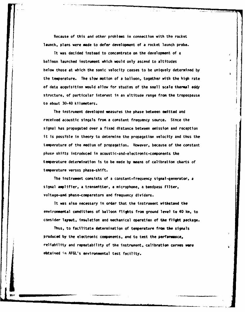
Because of this and other problems in connection with the rocket

launch, plans were made to defer development of a rocket launch probe.

It was decided instead to concentrate on the development of a

balloon launched instrument which would only ascend to altitudes

below those at which the sonic velocity ceases to be uniquely determined by

the temperature. The slow motion of a balloon, together with the high rate

of data acquisition would allow for studies of the small scale thermal eddy

structure, of particular interest in an altitude range from the tropospause

to about 30-40 kilometers.

The instrument developed measures the phase between emitted and 4received acoustic singals from a constant frequency source. Since the

signal has propagated over a fixed distance between emission and reception

it is possible in theory to determine the propagation velocity and thus the

temperature of the medium of propagation. However, because of the constant

phase shifts introduced in acoustic-and-electronic-components the

temperature determination is to be made by means of calibration charts of

temperature versus phase-shift.

The instrument consists of a constant-frequency signal-generator, a

signal amplifier, a transmitter, a microphone, a bandpass filter,

voltage-and phase-comparators and frequency dividers.

It was also necessary in order that the instrument withstand the

environmental conditions of balloon flights from ground level to 40 kin, to

consider layout, Insulation and mechanical operation of the flight package.

Thus, to facilitate determination of temperature from the signals

produced by the electronic components, and to test the perfornmce,

reliability and repeatability of the instrument, calibration curves wore

obtained in AFGL's environmental test facility.

i,

-11-

4. ACOUSTIC FLOW MEASUREMENT TECHNIQUES

It is shown in standard works on acoustics or physics

/e.g. Morse & Ingard 1968) that the velocity at which small disturbances

are propagated through a compressible fluid is given by the relation:

C2 (dP/aP)S (1)

where c is the wave propagation speed, p is the static pressure, p

the density, and s the entropy of the gas.

The temperature and velocity gradients produced in a fluid by

a sound wave are so small that each fluid particle undergoes a nearly

isentropic process. For purposes of computing the wave speed we assume

the process to be strictly isentropic and envoke the isentropic relation

for a perfect gas, p = const-p , where y(= Cp/Cv) is the ratio of the

specific heats.

We also use the equation of state of an ideal gas, pm = pRT, where

m is the molecular weight, R is the universal gas constant and T is

the absolute temperature. This gives an expression for c which is

independent of static pressure:

c = (yRT/m)l& (2)

On substitution of numerical values for the constants 7, R, and m

(for dry air) this equation reduces to:

c = 20, 067 TW (3)

where c is expressed in meters per second and T in degrees Kelvin.

We thus have a simple relation between the acoustic propagation

velocity, and the ambient temperature.

Having derived this fundamental relationship we must examine the

underlying assumptions.

The requirement that the wave Is adiabatic is only satisfied if the

incremental pressure due to the sound wave is very small compared to the

static pressure of the medium. This condition is met in the atmosphere

near the surface of the earth even with quite loud sounds. However, at

heights of 25 km the sound pressure from intense sources become an

appreciable fraction of the ambient pressure (19 torr - 2500Pa). There-

fore, if the sound impulse is transmitted at excessively high intensity the

velocity becomes a function of the ambient pressure and equation (1) is no

longer valid.

The signal picked up by the microphone at an ambient pressure

corresponding to 25 km corresponds to only about 0.5 Pa (down from about 20

Pa at atmospheric pressure). Thus we see that the amplitude employed is

small in comparison to the pressure at 25 km and that this requirement

imposes no practical limitation on the present investigation.

Another assumption is made in treating I as constant for a given gas or

mixture. For waves of very high frequency a velocity dispension w.r.t. the

sound frequency exists, the velocity showing an increase with frequency.

An explanation for this dispersion is given by Kneser (1933). It is based

upon the assumption that due to the great acceleration of the molecules

produced by the high frequency sound waves, energy imparted to the

molecules cannot be distributed among the various vibrational degrees of

freedom in accordance to equilibrium theory.

-13-

A small but finite "relaxation time" is required for a molecule to

adjust itself to a change in total energy imposed trom the outside. If the

sonic pressure changes act in too rapid succession, the molecule cannot

achieve equilibrium. Since y depends upon the specific heats, Cp and Cv,

and these in turn depend on the energy distribution among the various

translational, rotational and vibrational degrees of freedom of the

molecules, it follows that y cannot be regarded as a constant, but is a

* 6 frequency-dependent variable. Barret & Soumi (1949) point out that this

dispersion can be neglected when the sound frequency is less than about 500

kiloHertz.

Chen (1981) in his theoretical study on the feasibility of high

altitude atmospheric temperature probes, points out that when dispersion

occurs the ratio of the speed of sound at a certain frequency

to the speed of sound at zero frequency depends on both pressure and

temperature for a sound wave of a fixed frequency. Therefore, one

would need pressure information together with the speed of sound to

obtain the correct temperature.

In figure 13 of Chen's paper the speed of sound for a wide range

of frequencies is seen to double between altitudes of about 65 and

90 kilometers. It should be pointed out that increasing the altitude

also increases the mean free path of the molecules and thus has the

same effect on the ratio of the wavelength of the sound wave to the

mean free path as does increasing the frequency. Thus, the explanation

of Kneser above is thought to be relevant to the behaviour of the

propagation velocity found by Chen, and Chen points out that the influenceof relaxation should be studied.

During the course of the investigation it was decided that developing

a rocket launched instrument for studies of spatial temperature

distribution in the high atmosphere (60 to 90 kin) would be too difficult

and lengthy as a first project goal. Therefore, efforts were concentrated

on development of a balloon launched instrument for studies of the

microscale thermal eddies in the mid-atmosphere (in particular from 15 to

40 kcm). Below 60 km the propagation speed of a signal of the frequency

employed (8KHz) is equal to that at zero frequency and dispersion is

therefore not considered a problem.

That the acoustic speed is not dependent on pressure at these

altitudes (up to 30 kmn) has been verified in tests done at AFGL.

A third restriction lies in the fact that both y and mn must be

considered as functions of chemical composition of a gas mixture.

Atmospheric observations indicate that the composition of the atmosphere

remains substantially constant up to heights well in excess of 30 kin; with

the exception of water vapor and carbon dioxide.

The small carbon dioxide content of the normal atmosphere may be

neglected in this study. However, the water-vapor variation cannot be

neglected without causing appreciable error since the speed of sound in

pure water-vapor is much higher than in dry air.

It is possible to compute a correction factor based on the vapor

pressure of water, on the assumption that the speed of sound may be

regarded as a linear function of the relative concentration of the

components of a mixture.

This is done In Appendix I where it is found that 100 percent relative

humidity would cause 2"C error in a temperature measurement at 30*C, but

only 0.30C error at 00C. At -50*C the error is totally negligible and the

effect of water vapor is therefore not considered further. This agrees

with Barret & Soumi (1940) who state: "As in the case of ordinary virtual

temperature, the correction becomes small at higher altitudes in the

atmosphere and may be neglected above about 15000 ft." This will be

particularly valid even at ground-level in the first balloon flight which

is scheduled to take place in south-eastern New Mexico, an area not noted

for its high humidity. However, the effect should be kept in mind during

the first few thousand meters of ascent.

To measure the propagation velocity we consider a transmitter

and a receiver separated by a distance d (figure 1)

Fig. 1. Sound ray vectors showing the principle of sonic velocity

measurement (adapted from Kaimal & Businger (1963)).

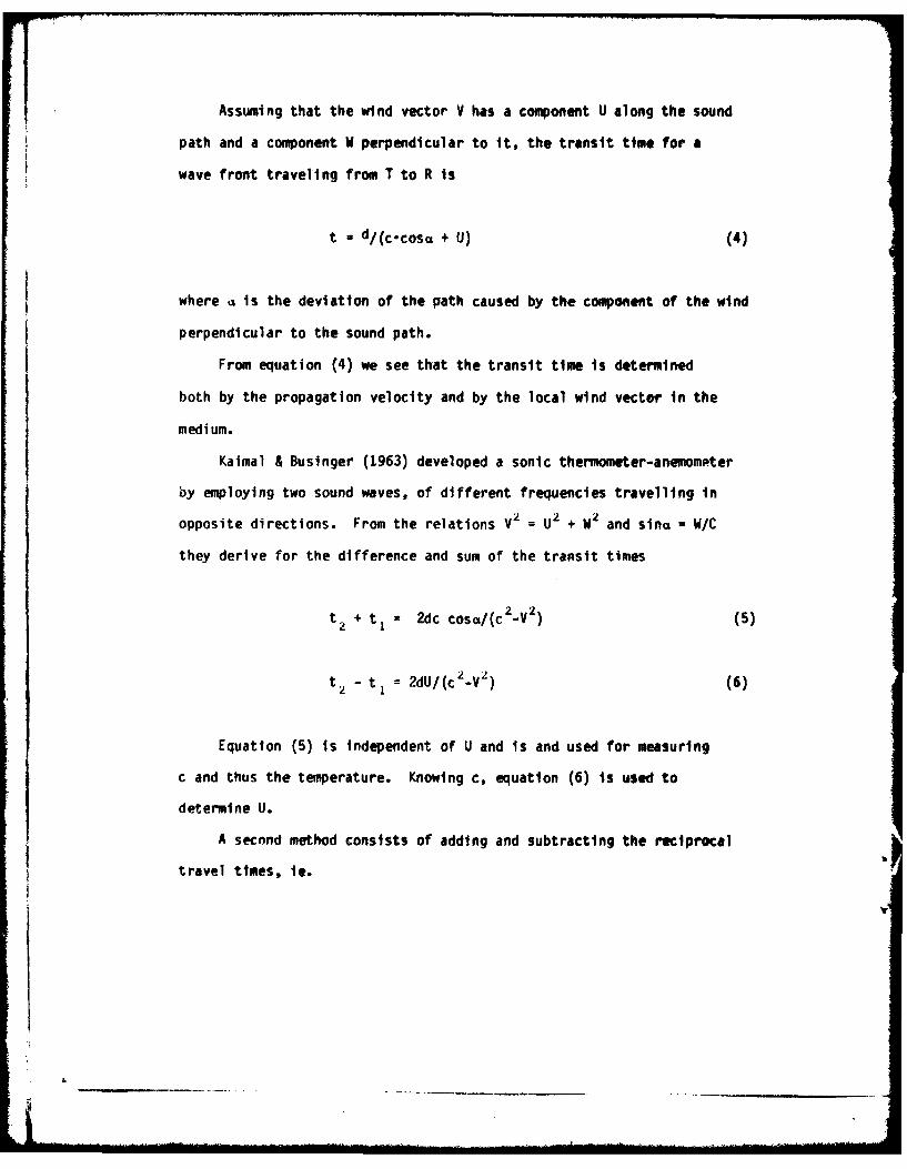
Assuming that the wind vector V has a component U along the sound

path and a component W perpendicular to it, the transit time for a

wave front traveling from T to R is

t . d/(c-cosa + U) (4)

where a Is the deviation of the path caused by the component of the wind

perpendicular to the sound path.

From equation (4) we see that the transit time is determined

both by the propagation velocity and by the local wind vector in the

medium.

Kaimal & Businger (1963) developed a sonic thermometer-anemompter

by employing two sound waves, of different frequencies travelling in

opposite directions. From the relations V2 = U2 + W2 and sin =- W/C

they derive for the difference and sum of the transit times

t 2 + t i = 2dc cosa/(c2 -V 2) (5)

t t I = 2dU/(c -V) (6)

Equation (5) is independent of U and is and used for measuring

c and thus the temperature. Knowing c, equation (6) is used to

determine U.

A second method consists of adding and subtracting the reciprocal

travel ttmes, ie.

-17-

t- +t' = 2 (c'cosu)/d (7)

t2 t 1 2 U/d (8)

Thirdly, the instrument of Larsen, Weller, and Businger (1979)

uses a phase-locked loop to keep the phase difference across the

soundpath constant, irrespective of wind and sound-speed variations,

by varying the frequency of the sound waves.

By assuming perfect phase lock they derive the equivalent expression

to (5)-(6) and (7)-(8):

(W - W0)/t0 + (WIi10)/10 = 2(c/c 0 cosa -1) (9)

- W0)/w0 - (= -, 10)/w10 ZU/c o (10)

were (w-wo) and (wl-uiO) are the differences between the actual transmitter

frequency and the free running frequency of the phase locked loop in the

two opposing directions.

Comparing these three sets of equations we observe that the phase-

locked loop method has the advantage that the path length d drops out

and that only measurements of relative frequency variations are necessary.

However, considered as a dynamic system a phase-locked loop, even

when phase-lock is achieved, is controlled by a highly nonlinear equation.

Consequently the system will become unstable if the phase difference across

the feed-back becomes equal to or larger than w radians, and also whenever

the transmitter frequency goes outside of the so called "lock-range" of the

phase-locked loop circuit. Prototype circuits using phase-locked loops

where tried out and severe problems of stability and loss of locks '.are

encountered. Because of the large temperature difference experienced wnienascending from ground level to 25 km in the atmosphere it would have been

necessary for the transmitter frequency to change from about 5 to 11 kHz if

the free-running frequency of the phase-locked loop was set at 8 KflZ.

Whereas this is possible, it requires that in this frequency interval the

phase characteristics of the transducers must be rather flat. Larsen,

Weller A Businger (1979) concludes that the only transducers fulfilling

this requirement seem to be condenser microphones. These transducers,

however, have a number of drawbacks, such as the need for a high bias

voltage (200 V) and special preamplifers. They would also only be capable

of producing sound of relatively limited amplitude, incompatible with the

strong attenuation in the mid and upper-atmosphere.

For these reasons it was decided not to pursue the phase-locked loop

principle but to concentrate on simple measurement of transit times from

the phase difference introduced by the acoustic path. Further details on

the phase-locked "closed-loop" principle can be found in Appendix V.

From the above it is noted that in the "inverse method",

equations (7) and (8), U measurements are not contaminated with variations

in c and W. However, since we are chiefly concerned with measurements of

c, which in all three methods is contaminated by velocity fluctuations, it

is not thought that going through the extra complication of trying to

obtain t 1 would result in any major improvement of the instrument during

the first few launches. Also, if required, the additional apparatus needed

-19-

to invert the measured transit times could probably be ground-based and

added at a later stage.

As has been pointed out, and as can be seen from equation (5) the

measured sound speed will be contaminated by the wind vector, V. This

will be considered in the following chapter.

I __ -__ __ _I__ __ _JLI__ __ __I _ __Ji__ __l_ ___I__ __ _

5. SONIC TEMPERATURE MEASUREMENT IN THE ATMOSPHERE

From equation (4) above the transit time for a wave to propagate from

the transmitter to the receiver is given as:

t = d/(C.cos a + U)

which with = sin- W/c becomes

c (W/c) 2 + U I'

Thus, the transit time is seen to be dependent both on the

wind velocity transverse to the soundpath, W, and along the soundpath,

U; as well as on the sound speed. However, since W/c < 1 we can ignore

the effect of W and set

t .. d ( +u -, (11)

The effect of the wind velocity along the soundpath is considered in

Appendix II were it is estimated that the error in temperature reading

would be 0.6*C and 3*C for mean wind velocities of 5 m/s and 20 m/s

respectively, with ten percent turbulent intensity.

This is a very serious error and on subsequent flights it will be

necessary to add another transmitter and receiver, with soundwaves of

different frequencies travelling in opposite directions, in order to

eliminate the effect of the wind fluctuations, U; as is outlined in the

previous chapter.

i

-21-

Neglecting this velocity contamination for the first launch of the

instrument we see that if the soundpath is chosen to correspond to an

integral number of wavelengths at some reference temperature To, we have

the transit time:

to = d/co = n/f (12)

where n is chosen.

For this temperature the phase difference across the acoustic

path is an integral number of 2% - i.e. zero. As the temperature changes,

the resulting change in sound speed will introduce an acoustic phase

difference. Thus, the transit time becomes

t = d/c = (n+ */2w)/f (13)

Integrated circuit phase comparators give an output voltage which is

proportional to cost and thus, for a single valued correspondence between

this output voltage and the measured temperature, the phase difference

across the acoustic path must lie between zero and 180 degrees.

Thence, the maximal and minimal sonic velocities that can be measured

are given by equations (12) and (13):

cmax co = d-f/n

cmin =d-f/(n+1/2) (14)

mn .

I m

We see that the maximum temperature range is obtained when the

receiver is only one wavelength away from the transmitter. This would,

however, require a very low frequency for the sound wave to travel across

an air sample of meaningful size. Also, choosing n to be very small would

give low sensitivity since there would be a large temperature change for

little phase change.

On the other hand, if we choose a very high transmitter frequency, n

will be a large number even for moderate propagation distances. This would

give very good sensitivity, but a small interval of temperature over which

we could measure unambigously.

Also, the attenuation of sound signals at low pressures requires that

the acoustic path be limited to some ten to twelve centimeters in order for

the microphone to pick up the transmitter signal at altitudes of 25 km and

above. This could of course be compensated by transmitting a stronger

signal, but a stronger signal would require much higher signal levels to

the transmitter and be incompatible with the weight and space limitations

of a balloon package.

Finally, d/e, the ratio of soundpath to transmitter diameter should

not be too much smaller than one as this would put the microphone in a

sound-field where the phase-change due to attenuation may not be

repeatable.

Considering all these requirements, a transmitter frequency of between

five and ten kilohertz was found to give both fair sensitivity and adequate

temperature range.

Becanse the electromagnetic transmitter (see chapter 6) was found to

produce a particulary strong signal for a-n eight kilohertz input this was

chosen as transmitter frequency.

-23-

Choosing an appropriate reference temperature and using equations (3)

and (14) we can calculate the measurable temperature range for given

lengths of the acoustic path. This is done in Appendix 111, from which we

sumrmarize four alternatives

Ref temp Acoustic path length Minimum temp Temp range for a +-v

a) 40*C d = xA40 = 4.43 cm -134 0C 1740C

b) 25-C d = 2,x25 = 8.66 cm -820C 1070C

c) 200C d = U 20 = 12.9 cm, -580C 780C

d) 00C d = 40. = 16.6 cm -570C 570C

Figure 2. Temperature ranges for different choices of length of acousticpath

From the physical properties listed in Appendix IV we see that the

expected temperature changes during flight will be from plus 200C at ground

level to minus 56*C at altitudes of 15 to 20 kilometers.

Thus alternatives a) and d) above have too large and too small

temperature range respectively. Letting d equal to 4X 0 would also make the

acoustic path too long to overcome the atmospheric attenuation.

However, choosing d equal to either 2X 25 or 3X 20 is seen to fit the

expected environmental conditions well. Alternative c) would have better

sensitivity but somewhat more limited temperature range than would

alternative b).

In order to make practical use of the above relations and results it

is necessary to (1) generate sound waves by electrical, or mechanical,

means; (2) transmit the sound through the atmosphere; (3) receive the sound

and convert it to electrical impulses; (4) express the time of travel of

the soundwave in terms of some electrical parameter; and (5) provide for

telemetry.

The last point is done by the telemetery unit at AFGL and will only be

briefly considered in Chapter 7 when performance estimates of the airborne

instrument are made.

In the following chapter we consider in more detail the first four

points.

-25-

6. THE BALLOONBORNE ACOUSTIC THERMOMETER (BAT)

As noted above the chosen design measures the phase shift of a

constant frequency sound wave over a fixed distance, rather than measuring

the frequency of a sound wave which has a fixed phase shift over a certain

distance.

The flight instrument, named BAT for Balloonborne Acoustic Thermo-

meter, employs a precision waveform generator using a crystal to control

the frequency of its sinusoidal output. A linear, bi-directional power-

operational-amplifier amplifies the sine-wave before it is converted into

an acoustic signal by a specially developed electromagnetic transmitter.

The acoustic signal is picked up, after having propagated across the air,

by a sensitive condenser microphone, and filtered through a narrow active

bandpass filter to remove the effect of any microphone pick-up from sources

other than the transmitter. The filtered signal and a reference signal

from the waveform generator are applied to voltage comparators that convert

the sinewaves into squarewaves, but do not alter their phase. This is done

to eliminate possible phase-errors introduced by small dc-offsets of the

sinewaves. Thus we have two 8 kHz squarewaves whose phase difference is due

to the passage of the signal through the acoustic medium and any phase dif-

ferences introduced by acoustic and electrical components. Assuming the

latter to be constant the change of phase difference between the signals

should be uniquely related to the temperature of the acoustic medium.

Originally the phase shifted waves were used as inputs to a phase

comparato;, the output voltage at which was passed on to a voltage

controlled oscillator which transformed the phase information into a

-26-

variable frequency and allowed for ease in interpretation of data using a

frequency counter and calibration curves.

However, after discussion with engineers from AFGL, the circuit for

the flight unit was altered slightly and the phase information presented

for telemetry to ground in three different forms.

Both the filtered signal and the reference signal are delivered for

telemetry after having been divided down from their original frequency by a

factor of 20. This is done both as a check of the electronic circuitry and

for possible application of signal processing techniques after receiving

the telemetered signals on the ground. The frequency division to 500 Hz is

made since no channels for telemetry are available at 8 kHz.

Both 8 kHz squarewaves are applied to an operational multiplier set up

as a phase comparator with a dc-level output which varies between plus and

minus w volts. Only signal levels between zero and ftve volts can be used

for telemetry and consequently the amplitude of the dc-signal is reduced by

one third in an attenuator and 2.5 volts added to it in a summing amplifier

before it is delivered.

Finally, a digital phase counter* uses flip-flops, a binary counter,

latches, digital gates and a high frequency clock to produce a digital

signal proportional to the phase shift. By using a 4 MHz crystal as clock

and letting the zero crossings of the two phase shifted signals determine

whether the counter is enabled or disabled this circuit gives 500 digial

counts for 360 degrees of phase shift.

A block diagram of this set up can be found in figure 3.

* This was developed by Gautham Ramohalli.

-27-

MITTEP )) L PHONE

AMPLIFR AMP F.[RAWIE

5cNAL-POWLRGENERATOR I.,UPPL'

VOLTAG E VOLT AGF

COMPARA. I COMPAA.

PHASE- , DC

COMP- LEVEL-ARATOR SHIFTER I

DIGITAL ._ _ _ _y__ DIGIALPHASE-MLTER _ _ _ _

I FREUN FRF.QL)INC.FREQUENG DI VIDEF

IFFER _.

'I ; A L

Figure 3. Block diagram of the Balloonborne Acoustic Themometer (BAT)

I,t * A

-28-

The route leading to the final design was by no means straightforward

and a variety of set ups, using partly different circuit components have

been tried.

A description of a "closed loop" feedback system using a phase locked

loop integrated circuit is given in Appendix V. This set-up is similar to

the one of Larsen, Weller and Businger (1979), mentioned previously.

Further details on the evolution of the final instrument are not

thought to be essential and are not included. The interested reader is

refered to internal memos AR 1042, AR 1044 and AR 1045 of M.I.T.'s

Aerophysics Laboratory as well as to the quarterly progress reports fur-

nished by the Aerophysics Laboratory to AFGL.

Below is given a fairly brief description of the individual com-

ponents. For a more detailed description with circuit diagrams and speci-

fications, refer to Apendices VI and VII, or to the "user-manual" supplied

to AFGL with the finished instrument.

THE ELECTRONIC COMPONENTS

The electronic circuitry, apart from the power operational amplifier

and relays, is placed on five 4x4" pc-boards which are connected to a con-

mon 50 strip bus line by cartridge connectors. Because of the large

changes in ambient temperature during a balloon flight, and to ensure

precision and reliability, high grade electronic components have been used

wherever possible.

For picthres of the circuit boards see figures 4 and 5.

The Generator board

This circuit board consists of nn XR 8038M precision waveform genera-

tor, set up to produce a low distortion sinewave. To ensure minimal

-29-

frequency drift the waveform generator is crystal controlled. Thus a 8 kliz

quartz crystal is set up to act as a parallel resonant device. This

crystal has an equivalent capacitance of 6 to 9 picoFarad. The generator

will free-run, without the crystal installed, at approximately 9.8 kHz and

will lock in on the quartz crystal which will then act as the primary

frequency control element.

Typical specifications for the generator board are:

Generator frequency: fp = 8000 Hz

Frequency calibration: ± 0.003% at +25*C

(equivalent to ± 0.24 Hz at 8000 Hz)

Drift with temperature: Parabolic curve centered at 25°C, with

negative temperature coefficient above and

below this temperature. Typically for

-250C < T < 50°C: Ap = ± 0.005%.

Temperature range of operation of electronic components:

-550C, +125 0C.

Distortion level of signal output THD = 0.5%.

The sinusoidal output signal is buffered using an operational amplifier to

eliminate unwanted feedback effects from other circuit components. The

output is passed on to the power amplifier and is also used as the

reference signal for phase measurement.

For more complete technical specifications and a circuit diagram of

the generator board see Appendix VI.

I

-301The power amplifier

The sinusoidal signal from the generator board is amplified by a

Torque Systems PA 112 linear bidirectional power op-amp to about 15 Watts

before being applied to the electromagnetic transmitter.

Operating temperature range of power amplifier: 00C to 500C.

The filter board

To remove any effect on the measured phase difference of acoustic

signals from sources other than the transmitter it was thought necessary to

pass the microphone signal through an extremely narrow bandpass filter,

centered at the transmitter frequency.

The filter chosen is a 2 pole (4th order) state-variable active band-

pass filter based on a general design given in "the Active Filter Cookbook"

by Lancaster (1975).

rhe filter consists of six high class operational amplifiers, L14 101,

and has the following characteristics.

Center frequency: f e = 8000 Hz

Amplification ratio for each stage (pole): Q, z Q2-10

Staggering value for maximum flatness in response: a -1.005

Staggered filter response e ot/e in 59 dB - 7 dB (insertion loss)

= 398.

Temperature range of electronic components -55*C, +125*C.

-31-

To avoid any interference by the filter on the microphone the

microphone signal is buffered before the filter input. After this buffer

the microphone signal is attenuated to avoid saturation due to the high

amplification ratio of the filter. The sinusoidal filter output is passed

on to a voltage comparator for transformation to a square wave.

A more detailed account of the filter board is given In Appendix VI.

The comparator board

Both the filtered microphone signal and the reference signal are

passed on to this board where they are converted from sinewaves to

squarewaves by two LM 111 voltage comparators. This is done because

voltage comparators operate at saturation and thus will produce constant

amplitude outputs (5 Volts), as long as the input amplitude is larger than

some threshold value (-4 mV). Hence, the voltage comparator outputs are

independent of the changing attenuation of the acoustic signal as the

balloon ascends and descends.

Also, if the microphone signal is small, any offset voltage, even if

very small, may alter its phase information. This will not be the case,

however, for the square-wave signal unless the offset is larger than half

its signal amplitude.

The phase information is extracted and presented for telemetry by

three different methods:

(1) Using two LM 14040B 16 stage binary counters, the 8 kHz signals

are changed to 500 Hz for telemetry. This was necessary to make the

signals compatible with available channels in the telemetry unit.

In dividing down the signal frequencies by a factor of 16 we also

reduce the phase shift between the signals by the same factor. Thus

instead of a maximum phaseshift of 180 degrees we get only 11.250.

-32-

However, the time-difference between the cycles is still the same (a 500 Hz

cycle is 16 times as long as an 8 kHz cycle!) and hence, if the signals can

be treated by timebased signal processing techniques, no loss of resolution

should result.

By tying the 250 Hz ouptut of the "reference-counter" to the enable

input of the "phase shifted-counter" the waveform of the phase-shifted

signal is modulated by the phase shift. This makes recording of the data

easier. In order to be able to calibrate out any phase shift introduced in

the telemetry equipment it was necessary to provide a possibility for

looking at the same signal on both telemetry channels simultaneously. This

is done by a switching relay, set up such that whenever a "command on"

pulse is applied to the instrument the reference signal will also be on the

channel which otherwise holds the phase shifted signal.

(2) Further, the 8 kHz signals are passed on as the inputs to an

XR 2208M4 four quadrant multiplier, set up as a phase comparator.

The differential dc voltage, V, at the two multiplier outputs is

related to the phase difference between the two input signals as:

V 0aK d Cos * (15)

where K dis the phase detector conversion gain. For input signals above

50 m0, K d is given by Exar as approximately 2 V/radian and is independent

of signal amplitude. Thus the phase comparator will vary from 3.14 volts,

at * equals zero degrees, to -3.14 volts, at # equals 180 degrees.

However, since only signal levels between zero and five volts are

acceptable for telemetry, the signal is passed through a difference -

-33-

amplifier, an attenuator and a summing amplifier where +2.5 volts dc is

added.

Both V and the two 500 Hz signals are buffered before being delivered

to the telemetry unit.

Temperature range of electronic components: -55°C to 125°C

For specifications and circuit diagrams of the comparator board see

Appendix VI.

The dgital board

(3) A digital phase counter, developed by Gautham Ramohalli*, has

been incorporated into the design. This circuit uses Motorola CMOS digital

logic circuitry and a 4 megaHertz crystal as a clock to count the number of

clockpulses between the cycles of the two 8 kiloHertz squarewaves from the

voltage comparators described above.

The 8 kHz signals are applied to dual type flip flops which enable and

disable a binary counter. Thus, when the first square wave goes high the

counter starts counting clockpulses. When the second squarewave goes high

the counter Is disabled and thus information about the phase between the

two waves now exists in the counter in the form of a digital number of

clockpulses counted. This 8 bit digital number is then latched into three

dual latches If enabled by a master sampler. The master sampler is derived

from the clock through a 24-stage frequency divider and can be changed for

*Now with Honeywell Inc., Minneapolis, MN.

-34-

compatibility with the telemetry equipment. It is presently set at one

Hertz, the expected transfer rate of the digital signal to ground.

After opening the latch gates the circuit waits two clock pulses to

ensure that the data have been latched in. Then the gates are closed so

that the data will not change as the counter is reset. Two more clock-

pulses are counted to make sure that the gates are closed, whereupon the

counter is reset and the cycle starts again.

It should be noted that this digital counter is capable of delivering

digital phase information at rates approaching & kHz if the master sampler

is changed appropriately, and also that it operates over 360 degrees of

phase shift.

The digital circuit components used include MC 14011B NAND-gates,

MC 14013 Dual type flip flops, an MC 14040B Binary Counter, MC 14042B Quad

latches, MC 14049B Hex buffers and an MC 14521B 24 stage frequency divider.

The temperature range for these components: -400C to +750C.

For more information, specifications and a circuit diagram of the

digital board, see Appendix VI.

The regulator board

The circuitry described above operates between ± 12 Volts with the

following exceptions:

- the power amplifier requires ± 24 V;

- the voltage comparators and binary counters are set up to work

between +5 Volts and ground to make the level of the 500 Hz

signals compatible with telemetry requirements;

- all digital circuitry works off + 5 Volts.

-35-

The airborne power supply will be 23 times 1.5 Volt batteries,

initially delivering 1 34.5 Volts. This is regulated down to ±t 24 Volts,

1 12 Volts and + 5 Volts, using Motorola voltage regulators of the MC 78-

and MC 79-series. The use of voltage regulators ensures a constant supply

voltage as the batteries use up part of their charge throughout the'flight.

The power requirements for the electronic circuitry is only some one

hundred milliAmperes at most. The power amplifier delivers about 15 Watts

at 1 24 Volts to the transmitter. From specifications about power

dissipation at max supply (60 Watts) the amplifier should draw well under

24 Watts, which would be equivalent to 1 Ampere.

The voltage regulators are rated for 1.5 Amperes continuous supply but

because of the harsh environment, and to minimize the possibility of power-

failure, the regulators were set up for much less than full load. Thus two

pairs of regulators are set up in parallel to supply plus and minus 24

Volts to the amplifier only. The outputs of these regulators are connected

by diodes to avoid current flow between them due to small differences In

the regulated voltage.

To supply the electronic components the plus and minus 24 Volt regula-

tors are powering ± 12 Volt regulators, the + 12 Volt regulator supplying a

+ 5 Volt regulator.

The voltage regulators have been tested at AFGL In temperatures down

to -600C. When turned off and allowed to cool down to ambient temperature,

they required some 20 seconds before regulating the correct voltage level

when turned on again.

For specifications and circuit diagram of the regulator board see

Appendix VI.

-36-

yiqre . Cmpoentside Of the electronic

circuit boards

-37-

-j~ MO

~j~Ur 5* everse side 0f the eectrolc

-38-

THE ACOUSTIC COMPONENTS

To overcome the severe attenuation experienced during ascent through

the atmosphere a transmitter capable of producing a fairly intense acnustic

signal Is required.

In the first year of this program an electrostatic transmitter was

developed and shown to be capable of producing the necessary signal ampli-

tude for use up to 90 km of altitude (see Chen (1981)). However, repeated

problems with arcing across the aluminized Mylar film rendered this

transmitter far too unreliable for airborne testing purposes.

Commercially available speakers of type JBL 2105 were tried and found

to give the required amplitude. But during tests in the Aerophysics

laboratory they were found to have inconsistent and unrepeatable phase

characteristics. Thus, the phase difference measured when cooling the

acoustic path, and transmitter, down was not the same as that measured at

the same air temperature when letting the medium warm up.

It is believed that this is because these speakers employ viscous

suspension of the transmitter cone to its casing. The viscosity of the

suspending substance would most probably change with temperature, with a

delay relative to the ambient temperature, and this would explain the

observed change in phase characteristics. However, the change of viscosity

is likely to be dependent on localized temperature varia'Io%s across the

transmitter surface due to both the rate of cooling of the medium and the

power dissipation, thus accounting for the unrepeatability.

Consequently it was necessary to develop and test an alternative

transmitter.

-39-

The electromagnetic transmitter

The designed transmitter relies on electromagnetically induced

vibrations for its sound production. An aluminumized-Mylar laminated film

has been etched such that only a conducting spiral pattern remains on the

Mylar surface. This diaphragm is suspended in the fringing radial field of

a Samarium-Cobolt permanent magnet disc.

The magnetic disc is centered inside an aluminum drum and mounted to

the top of an adjustable screw which is attached through the back-surface

of the drum casing. Thus the distance between the magnet and the mylar

membrane is adjustable, since the membrane is stretched tightly over the

top of the drum by an aluminum ring. The attachment method being totally

independent of any viscous suspension is thought to be of great importance,

as mentioned above.

The spiral pattern membranes were constructed at AFGL by sensitizing,

photographically exposing, developing and etching aluminized mylar film of

total thickness two thousandths of an inch.

The amplified sine signal from the power amplifier is passed on

through the magnet support screw and the magnet and then through the con-

ducting spiral to ground potential in the drum casing. Since an alter-

nating current is passing through a magnetic field that has a component at

right angles to the conductor the resulting electromagnetic force causes

the mylar film to vibrate at the frequency of the ac-signal.

The transmitter proved to have a highly frequency-dependent amplitude

response. This, however, is not a major concern since the present instru-

ment employs a constant frequency transmitter signal. The output charac-

teristics of the speaker were nearly independent of membrane tension. The

j

-40-

distance of the magnet from the membrane had a somewhat stronger effect on

the output and a spacing of some one fifth of an inch was found to give the

largest amplitude.

Furthermore, the position of the magnet strongly changes the phase

characteristics of the transmitter. This is to be expected since moving

the magnet will change the ratio of the radial component to the axial com-

ponent of the magnetic field which pass through the diaphragm. Since the

radial component induces axial vibrations and the axial component seeks to

induce radial components the deflection mode of the diaphragm will change,

thus altering the phase characteristics.

Typical performance of the electromagnetic transmitter, when tuned for

*8000 Hz, which turned out to be one of many "resonant peaks", was found to

be 2 Volts of signal picked up by the condenser microphone at atmospheric

pressure when a 10 Volt signal (15 Watts) was applied to the transmitter

* and the sound path was some 10 cins long. This gives a -14 dB fall off due

to the transmitter, the microphone and the acoustic path.

At the lowest pressure tested, 10 mbdr, corresponding to some 31 kms

of altitude, the falloff ratio was -54 dB. This is equivalent to a

microphone signal of 21 mV, which when applied to the filter input gave

some 0.2 V filter output and resulted in proper operation of the phase

measuring part of the circuit.

The transmitter was cooled down while operating at AFGL in order to

test its ability to withstand the expected environmental conditions. At

an air temperature of -600C the transmitter was shut off and the diaphragm

allowed to cool down to air temperature. When reapplying the amplifier

signal the transmitter was found to consistently resume operation.

For specifications on the transmitter see Appendix VII.

-41-

The condenser microphone

To pick up the acoustic signal, which may be strongly attenuated from

passing through a low density medium, use of a microphone of very high sen-

sitivity is necessary.

The microphone used, a Bruel & Kjaer Type 4165 condenser microphone

with a half inch diameter cartridge, has a sensitivity of 50 millivolts per

Pascal pressure change. With the microphone signals mentioned above this

corresponds to ratios of sound pressure to sea level atmospheric pressure

and 30 km atmospheric pressure of 4.10 -4 and 3.10 -4 respectively. Thus,

the requirement of low sound pressure relative to ambient pressure,

examined in the theoretical analysis, is met.

The microphone is attached to a Bruel & Kjaer Type 2619, half inch

preamplifier. The microphone cartridge needs 200 Volts dc polarizatrion

voltage on one side of its diaphragm for operation. This, as well as 28

Volts dc needed to power the preamplifier, is supplied by a B&K Type 2804

Microphone power supply which in turn is powered by three 1.5 Volt alkaline

batteries. Ths power supply is capable of driving two microphone/pre-

amplifier units for 40 hours before change of batteries is necessary.

The microphone power supply also serves as an adapter for passing the

microphone signal from B&K's microphone cable and plugs onto a Bnc

connector.

Some important characteristics of the microphone, pre-amp and supply

are:

Microphone, B&K 4165 --

Open circuit sensitivity 50 mV/PaTemperature coefficient(between -50C and +600C) 0.0012 dB/OC (-100 ppm)

-42-

Influence of realtive humidity <0.1 dB(in absence of condensation)

Preamplifier, B&K 2619 --

Maximum sinusoidal output voltage 4V rms

Power supply, B&K 2804 --

Signal attenuation 0 dBTemperature range 00C to 40°C.

The microphone and preamplifier were tested and found to operate nor-

mally down to temperatures of -600C.

For more detailed specifications of these components see Appendix VII.

For pictures of the electromagnetic transmitter and condenser

microphone with Its preamplifier attached, see figure 6.

-43-

Figure 6. Front view of the electromagnetic transmitter and

condenser microphone

- | 1 1 I I : :- - -- I

-44-

THE CASING AND INSULATION

The electronic components described above plus the power supply for

the condenser microphone'are contained in a 17xl5x6u aluminum chassis box

with a removable aluminum top surface. A hinged lid is placed in the top

surface and this lid opens to allow easy access to the circuitry. For ease

of transportation the chassis box is equipped with a removable

carrying-handle.

The five circuit boards are inserted in Scotchflex cartridge connec-

tors that are tied together with a 50 line bus strip. This allows easy

interconnection of the boards, which can be removed from the chassis box

individually for maintenance and troubleshooting. The multistrip is

attached in the middle of the chassis box floor with the microphone power

supply and power amplifier on each side.

One of the "end walls" of the box hold all the electrical connections.

Thus, plus and minus 30 Volts supply voltage and ground are received

through three Bnc connectors. Seven additional Bnc connectors deliver and

receive various signals for connection with the acoustic components,

telemetry and for troubleshooting. They are, the power amplifier signal to

the transmitter; the filter input to the bus strip from the microphone

supply; the dc voltage from the phase comparator and the two 500 Hz signals

for telemetry; and the oscillator-and filter outputs for troubleshooting.

Also, a 4 foot multistrand cable with a 26 pin Bendix connector is

passed out of the chassis box to the telemetry unit. This cable and Bendix

plug holds the eight bit digital signal for telemetry; connections for the

*on" and "off" commands for the power supply of the flight instrument; and

two free connections that can be used to obtain information about, and

monitor, the temperature in the chassis box. The "on" and 'off" commands

.

-45-

are applied to a latching relay which is connected up in parallel with the

switching relay described in the section on the comparator board.

For pictures of the chassis box with the electronic circuitry

installed, see figures 7, 8 and 9.

For more details on the flight instrument, with wiring diagrams and

scale drawings, refer to the Instruction Manual for "Ballonborne Acoustic

Thermometer," to be delivered with the instrument to AFGL.

The question on whether and how much insulation will be needed is far

more complex than it might seem at first sight.

The instrument, on ascent to altitudes of 25 kms will be exposed to

temperatures ranging from ground temperature (-20'C) down to about -560C.

The transmitter and receiver have been tested and found to operate satis-

factorily in this temperature range. This is also the case for the voltage

regulators.

Most of the electronic components are of milspec rating with

operating temperature ranges down to -55*C. However, the PA 112 power

amplifier and the B&K 2804 power supply are only rated down to O°C.

It is important to remember that because of radiative heating in the

atmosphere, the temperature of the gondola of the balloon and of the

instruments attached to it will not be the same as the temperature of the

surrounding air. Experience from previous balloon flights of AFGL indicate

that the temperature in the gondola can be as much as 60 to 700C above

ambient in flights to about twenty kilometers altitude. Thus it is feared

that power dissipation may cause certain of the electronic components, in

particular the voltage regulators, to overheat and malfunction if the

flight instrument is insulated too thoroughly.

it

-46-

Calculation of the expected heat transfer and temperatures across the

walls of the chassis box was attempted by following the methods described

by Lichfield A Carlson (1967). This analysis can be found in Appendix

VIII. However, their procedure involve far too many uguesstimates" of

factors like "percentage of flight package being exposed to sunlight" to

give any meaningful answer.

Correspondingly it is believed that the only possible method of

dealing with the question of insulation lies in actually trying the

instrument out in the atmosphere. The electronic components have been

moderately insulated by surrounding them with foam. (As can be seen in

figure 9; note in particular the complete enclosure of the microphone

power supply.)

If necessary it is possible to wrap the chassis box and surrounding

gondola with aluminized mylar as a radiation shield, and /or heat the non-

wnilspec electronic components using the excess heat from the voltage

regulators.

Both the attachment of the chassiz. box to the gondola and the support

boom for positioning the transmitter and microphone some distance away from

the gondola have been designed by Richard Borgesen at AFGL.

The mounting for the chassis box is to be by means of screw-rivets to

a mounting bracket.

The transmitter ard receiver are to be held rigidly with respect to

one another in a craddle which thus ensures that the acoustic path is of

constant length. It will however be possible to adjust the length of the

acouistic path to compensate for any constant phase shift in the acoustic-

and electronic-components.

-47-

The craddle holding the acoustic instrumentation will be positioned

about four feet from the gondola at the end of a telescopic retractable

am. The balloon will take off with the arm extended but on coming down to

land the telmetry comnand to deploy the parachute will cause a

constant-torque* spring to retract the arm and pull the craddle inside of

the gondola. (See figure 7 for a picture.)

More details on these components will be found in the instruction

manual for the instrument.

The weight of the chassis box and electronic components is soe 10 to

12 pounds, whilst the transmitter and microphone weigh less than 5 pounds.

Thus, the total weight of the experimental equipment, including the

craddle, chassis box mounting and retractable arm, as well as batteries for

the 1 35 volts power supply, is estimated to be well under 75 pounds.

-48-

Figure 7. The arm for holding the acoustic components

-49-

Figure 8. Exterior

view of the flight instrument

iOA

-50-

Figure 9. Interior view of the flight instrument

-51-

7. TEMPERATURE MEASUREMENT

We now calculate the expected sensitivity of the three telemetry

signals containing the air-temperature information.

The dc voltage from the phase comparator varies between zero and five

volts. Taking 10 m as a representative number for the smallest meaningful

voltage change (this is also suggested as a typical value of the noise

level in telemetry) we get as a rough estimate of the sensitivity for the

different acoustic paths considered in chapter 5.

x ATttI AV/oC ATin for AV

b) 2x25 1070C 47 mV 1/5 OC 9.3 mV

c) 3 20 780C 64 m 1/6 -C 10.7 m

d) 4.0 570C 87 mV 1/8 °C 10.9 mv

Fig. 10 The expected sensitivity of the phase comparator output

The digital phasemeter uses a 4 MHz clock to count the phaseshift

between two 8 kHz signals and thus produces 500 counts for a phase shift of

one full cycle. Consequently we have 250 digital bits for 1800 of phase

shift which results in the following sensitivities.

x bit/°C °C/bit

a) 2x25 2.3 0.43

b) 3 20 3.2 0.31

c) 4Ao 4.4 0.23

!0

Figure 11. The expected sensitivity of the digital phase meter output

±IiI-

-52-

For the modulated 500 Hz signal the full scale difference

corresponding to 180' of phase shift between the 8 kHz signals will give

11.25° of phase shift. This corresponds to 0.10, 0.150 and 0.20 of phase

shift per degree centigrade of temperature change for alternatives b), c)

and d), respectively.

Had the instrument been ground based these sensitivities could have

been realised with rates of data aquisition of 8000 times per second.

However, in the telemetry process some of the sensitivity and much of the

rapidity is lost.

Thus the phase comparator voltage can only be telemetered twice per

second and with a maximum accuracy of about 0.2 OC. The digital signal

will only be available once every second with the sensitivity halved due to

telemetry. The 500 Hz signals, however, can be telemetered continuously.

Since the limiting sensitivity of the signal which has the highest

resolution, the phase comparator signal, is set by telemetry we see from

figure 10 that the obvious choice of acoustic path is b). This choice

qives the largest temperature range, in case anomalous atmospheric con-

ditions are encountered and also has the shorter acoustic path, giving the

least attenuation of the acoustic signal.

This choice gives the following specifications for the instrument:

Length of acoustic path x = 2x25 = 8.7 cm (3.41")

Phase comparator signal Twice per second with 0.2°C accuracy

Digital phasemeter signal Once per second with 0.80C accuracy

Continuous wave signal Continuous with unknown accuracy(would depend on method of datatreatment)

Figure 12. The expected behavior of the final design

-53-

In the previous estimate of the response we assumed that all signals

vary linearly with temperature over the complete temperature range.

However, this is not an exact assumption since the temperature is propor-

tional to the square of the sound speed. Moreover, the most sensitive

signal, the phase comparator output voltage, changes as the cosine of the

temperature induced phase change.

To indicate that this does not seriously affect the above assumptions

we present below the derivation of the exact response of the dc-level

telemetry signal from the phase comparator for a one-dimensional source.

Denote

T temperature

c soundspeed

x wavelength

d acoustic path length

f frequency

A phase difference across the acoustic path

Oc phase difference across the acoustic and electroniccomponents

OT=A+¢c total phase difference as seen by the phase

c omparator

Let subscript zero denote reference conditions

-54-

At To:

Initially set the acoustic path length d - 2x0

The resulting output of the phase compactor #T = +c

Increase the acoustic path by a distancex such that T = 0

Thence, we can write the acoustic path as -

d = 2x + x= + * )/2n) X (16)

At some general temperature T, the phase comparator will see

T = A + Oc

and thus the acoustic path length can be written as

d = 2x + x + - A271 +(17)

4 it + ' c + A

d-2xEquating (16) and (17) and writing *c as ) 2n we get

upon rearranging-

A 2n (d/x) 1o/X,-11 (18)

We now use equation (15) for the phase comparator voltage and

A0/A = c0/c = (T /T)I/2 , to get

V K cos[2Pj(d/xo)((To/T) - 1] (19)

* d 0o

The manufacturer, Exar Inc., gives the phase comparator conversion gain of

their XR 2208 integrated circuit component as "roughly 2V/rad." It has

been found however, during testing of the circuitry, that 3.7 Volts is the

-55-

exact value. Thus, the equation for determining the attenuated, dc-shifted

telemetry signal as a function of the ambient temperature becomes

V+ 2.5)

= [. 1 + cos(2w{(d/x )((T /T)/ ' )j' (20)

Equation (20) is plotted as V vs. T for T = 25*C in figure 13 where it

can be seen that it approximates closely the following straight line

segments

Temperature range Slope AT min

-65*C to -15*C 70 mV/*c 1/70C

-15°C to 50C 38 mV/*c 1/4-C

5°C to 250C 14mV/*c 1°C

Thus we see that over most of the expected temperature range (above an

altitude of about 5 km), the one-dimensional theory predicts that the

telemetry equipment will set the limit to the attainable sensitivity.

Having chosen a final design we go on now to consider the

environmental testing and calibration of the finished instrument, the

problems encountered, and their subsequent solution.

- ... . .. . . ..A. . . . | .. II. . ..""°" . ..

-56-

'

0 1* .. ...

o * .. . ".... 4. i. .

U I

z . ,

-- .. ..... .. .% ,o.

N '

it

*00

4 rO I

* I

Figure 13. The one-dimensional theoretical response of the dc-teleaetrysignal.

-57-

The environmental testing and calibration of the instrument took place

in AFGL's low-pressure chamber. This chamber allows for temperature

control by cooling the chamber walls with liquid nitrogen. The flow of

nitrogen, through channels in the walls, is controlled by an adjustable

thermostat. Thus it was believed that the environmental conditions

encountered in flight could be closely modelled.

The acoustic components were tested in the chamber with the necessary

electrical signals fed in through connections in the chamber walls. When

the temperature was lowered to -580C both the transmitter and the

microphone were operating satisfactorily. The amplified sinesignal was

disconnected from the transmitter and the temperature of the diaphragm

allowed to cool down to that of the ambient air (-57*C). When the

transmitter signal was reapplied after some 15 minutes, the transmitter

resumed normal operation.

With an acoustic pathlnnmgth of some four inches, the amplitude of the

received microphone signal was found to be sufficient for operation at

least down to 10 torr (corresponding to an altitude of about 30 kin).

Furthermore, the observed phase difference between the transmitted and

received signals, as displayed on a dual-beam oscilloscope during the

environmental test, did not seem to be a function of pressure. This agrees

with Chen's (1981) findings as noted in chapter 4.

The chassis box containing the electronic components was placed in

the temperature chamber and found to operate satisfactorily down to -20*C.

When the temperature, as measured inside of the box, was lowered to -22*C

the instrument malfunctioned. The reason for the malfunctioning seemed to

be failure of the microphone power supply due to the alkaline batteries

being too cold. However, when the temperature of the instrument increased

-58-

to -15*C normal operation resumed.

It is important to recall that due to radiation heating in the

atmosphere the temperature of the chassis box is not expected to fall as

low as -20C. Experience from previous launches indicate typical gondola

temperatures of around O*C at altitudes of 20 to 30 km's. Also, as noted

in the previous chapter the dissipative heating from the voltage regulators

causes the chassis box to be at a temperature considerably above that of

the surrounding medium, and thus it is not thought that cooling of the

electronic components and power supply presents a serious problem.

For calibration of the flight instrument the chassis-box was

positioned outside of the temperature chamber, which thus contained only

the transmitter and microphone, as well as the temperature sensors used for

reference. This was done to obtain a more uniform temperature field and

slower changes of the air temperature in the acoustic path. For a picture

of the calibration set-up see figure 14.

The temperature sensors used were; 3 copper-constantan thermocouples

(wire diameter of about 1 mm), 1 iron-constantan thermocouple (#40, wire

diameter of about 0.05 mm), 2 thin film and 2 bead thermistors*.

Initially all eight temperature sensors agreed (during set-up and

adjustment of the acoustic path, with T = 25*C). However, once the

temperature was lowered it soon became evident that the above temperature

sensors had a much slower response to temperature changes than that

indicated by the output of the flight instrument with equation (20).

*(Omega Products, Hartford, Connecticut).

-59-

Figure 14. The set-up for calibration at APGL

ili I I

-60-

The problem of slow response of the thermocouples and thermistors

remained at all temperatures. In particular, when cooling the chamber down

the discrepancy was found to be large. Consequently, all calibration data

was taken while the air in the chamber was allowed to warm up from a

minimum temperature by conduction through the chamber walls.

The resulting calibration data, with the linear estimate and the

prediction of equation (20), is given in figure 15. It should be noted

that the difference between the experimental points, which were obtained

using thermocouple readings, and the theoretical estimates is less than the

difference between different thermocouples and thermistors (which at times

read as much as 10 to 15*C differences.)

It must also be remembered that equation (20) is a one-dimensional

result, assuming a point source transmitter. In reality the transmitter

is of finite size (4" diameter) and any accurate theoretical prediction

would be, at best, complicated.

Therefore, it is believed that the discrepancies do not point to any

deficiency of the instrument, but rather show that measurement of the sound

speed indicates temperture changes much more rapidly than does the

thermocouples and thermistors employed.

In order to resolve this problem satisfactorily additional calibration

using finer thermocouples would be necessary. However, since the

launch-date for the planned first flight test of the instrument is

approaching rapidly it was decided to postpone this until after the flight.

Two possibilities exist for obtaining a reference for the data of the first

flight.

(1) Attempts to calibrate will be made at the launch site (Hollomn

AFB, New Mexico). Since the night and day temperatures my fall down

-61-

IL.!1

zV0W

Ix<

1 <0

L

T-Q:

Fiur 5. Th eslt f albato wthteoetcl reitin

-62-

below freezing and reach 25 to 300C respectively a partial calibration

curve could be constructed.

(11) The one dimensional analysis leading to equation (20) could be

used as a "best approximation" during the first flight.

It would be necessary to choose some reference temperature, To,

and calculate the resulting xo; adjust the length of the acoustic path

to make the phase difference between the comparator inputs, *T' zero.

Then, measuring the length of the acoustic path, d, we could apply

equation (20) to find the air temperature from the dc-level telemetry

signal.

This has been done for To = 25% and d = 2x s for every degree cen-

tigrade from +29* to -84%. The result of the "theoretical calibration" is

plotted in figure 13, detailed results can be found in Appendix IX.

Since the position of the transmitter and microphone in the afore-

mentioned craddle is thought to slightly alter the phase characteristics of

the acoustic path, it will be necessary to carry out the final calibration

once this craddle is available from AGFL.

Furthermore, it is proposed to calibrate the digital phase signal

against the dc-signal during the first flight.

-63-

8. METEOROLOGICAL SIGNIFICANCE

At this stage it seems appropriate to quote from one of the earliest

papers on sonic thermometry. In 1948, Earl Barret and Verner Suomi of the

University of Chicago undertook a study sponsored by the Signal Corps

Engineering Laboratories to develop "...practical equipment which can be

utilized in routine balloon soundings from the ground to altitudes of about

30 km." The instrument they developed used short pulses of high frequency

sound,generated by applying a pulse voltage to a piezo-electric crystal.

Whether their laboratory model was ever balloon-launched is not known to

the present author, but in their 1949 J.A.M. paper they sum it up

beautifully:

Having shown that it is possible to automatically andremotely measure the velocity of sound at various levelsthroughout the free atmosphere, it becomes desirable to indicatethose special advantages which accrue from the use of thistechnique as contrasted with other methods of temperaturemeasurement now employed. The foremost of these advantages,from the viewpoint of higher-atmosphere sounding, arises fromthe almost complete indifference to radiation effects resultingfrom the sonic technique. All existing thermometer devices withwhich the writers are acquainted make use of some piece ofmatter as a measuring element, with the assumption that thispiece of matter is in thermal equilibrium with the atmosphere inits vicinity. The actual measurement involves a determinationof the numerical value of some physical variable quantitlywithin this piece of matter, with the supposition that a uniquecorrespondence exists between this variable (electricalresistance, volume, density, thermal e.m.f, etc.) and the"temperature" of the surrounding air. Because of the fact thatthermometers of these types have been most useful practically,physicists and engineers have defined "temperature" in terms ofthese physical variables inside the piece of matter used in thethermometer.

Experience in~dicates that for a very large number ofapplications these techniques and definitions are satisfactory.For the case of atmospheric temperature in particular, however,care muist be exercised, since the piece of matter may be actedupon by two principal physical variables. The first of these isthe air temperature, which for purposes of this paper will be

-64-

defined as being directly proportional to the mean translationalkinetic energy for a large number of air molecules. In theabsence of any other physical forces or energies, experience andthermodynamic considerations indicate that the moleculescomposing the thermometer will, in time, acquire energy from theair until the net trdnsfer of energy between air and thermometerapproaches zero. Under these conditions, the internalproperties of the thermometer may be considered as uniquelydetermined by the energy of the surrounding air, i.e., the airtemperature. However, as the instrument ascends higher into theatmosphere, the number of molecules which can exchange energywith the thermometer decreases, while another physical factor,namely radiant energy from the sun, becomes more prominent.This radiation is capable of supplying energy to the thermometerquite independently of the effect of air molecules. In thelimiting case, the effect of air molecules approaches zero andthe "thermometer" becomes a pyrheliometer or bolometer andmeasures *temperature" at which energy gained by radiationequals that lost by radiation. Thus it is clear that twoconflicting definitions of temperature at a point in theatmosphere can exist and that ordinary thermometers cannotclearly distinguish between them. Practical devices such asradiation shields and highly reflective coatings serve to reducethis ambiguity but cannot entirely eliminate it.

In contrast to the conventional thermometer, the sonicthermometer yields a measurement based upon the very propertywhich is used to define molecular temperature, namely themolecular energy of the air. Since it is unnecessary to utilizean intermediate step involving the internal properties of apiece of matter, the ambiguity in the meaning of "temperature"is reduced. Thus the introduction of sonic thermometers wouldtend to reduce the confusion which confronts physicists of thetipper atmosphere who attempt to abstract information fromordinary radiosonde data at high levels.

The second major advantage may be considered as a corollaryof the first. Since no piece of matter acts as an Intermediaryin the measurement, the time lag associated with ordinarythermometers is not inherent in the sonic technique. Notransfer of "heat energy" from air to thermometer, with theusual exponential relationship to time, is required. A time lagdoes exist, but the magnitude of this lag is of the order of0.001 sec; that is, the time required for one pulse to travelthe fixed distance. Thus, the sonic technique is highly suitedto measurements of temperature where the temperature varieswidely in short time intervals. This feature makes thetechnique invaluable for micrometerological studies oftemperature variations.

-65-

A third advantage obtainable by the sonic techniqueinvolves the property of space integration which is inherent inthe method. Because of the high velocity of sound waves it ispossible to lengthen the distance through which the soundtravels to fairly large values, of the order of hundreds ofmeters. If the atmosphere through which the sound passes is nothomogeneous in temperature, the temperature indicated by thesonic method represents an average over the travel distance.The integration cannot be considered as absolutely independentof time, of course, since the velocity of sound cannot beinfinite; however, the time interval over which the integrationis made is so small in comparison with the rapidity of localtemperature fluctuations in the atmosphere that for practicalpurposes the measurement may be regarded as a space integrationmade at a particular instant of time. Such space integrationsmay be of value in determining representative surfacetemperatures of air masses by elimination of the local effectswhich affect "spot" temperature measurements at weather stationsand by at least a partial averaging of such variations intemperature as are due to local ground heating and/or turbulentmotion along the path.

-66-

9 CONCLUSIONS AND RECOMMENDATIONS

An airborne sonic thermometer has been designed and developed and now

appears ready for testing in the atmosphere. Flight tests, using balloons

to carry the instrument to altitudes of 25 to 30 kilometers, are planned.

The instrument incorporates a specially developed electro-magnetic

transmitter, a very sensitive condenser microphone, Integrated circuit

components and a small power amplifier. The balloon launched instrument

consists of an aluminum chassis box wV".h a purpose-built craddle holding

the transmitter and microphone on the end of a four foot retractable arm.

Tests have shown that the intensity of the sound produced by the

transmitter makes the instrument capable of operation to altitudes of at

least 30 kilometers. Also, the components of the instrument are thought to

be able to withstand the changes of ambient temperature met in flights to

these altitudes.

The instrument produces information about the ambient temperature in

three different forms

(1) A dc-voltage level varying between zero and five volts.

(2) A digital 250 bit signal.

(3) Two phase shifted 500 Hz signals.

The sensitivity of signal (1), as indicated both by theoretical

calculations and by calibration is thought to be about 0.20C over a temper-

ature range of 105*C, from +251C to -80°C.

The corresponding sensitivity of the digital signal will be some

0.8°C; whilst the sensitivity of 500 Hz waves will be determined by the

chosen method of signal processing.

-67-

The temporal resolution of the instrument is set by the transmitter

frequency, 8 kHz. However, for balloon launched operations the telemetry

of the signals back to ground will be a practical limit. In the first

scheduled flight the telemetry rate has been set at two hertz for signal

(1) and one hertz for signal (2), whilst signal (3) will be transmitted

continuously.

In its present form the instrument suffers from the effect of velocity

contamination of the measured acoustic propagation velocity which can cause

errors of up to one degree centigrade in the measured temperature. To

eliminate this error it is proposed that a second sound path, with an

acoustic signal of a suitably spaced frequency to avoid signal crosstalk,

be incorporated in the next design. This would allow simultaneous

measurements of the ambient velocity and temperature and accurate

determination of quantities like flux Richardson number and turbulence

structure-constant should be possible.

Another difficulty concerns the need for a better calibration

technique. The available calibration, whilst confirming thle overall

response and measuring range, is too erratic and unrepeatable to be used

for accurate temperature determination. Thus it is proposed that during

the first flight the instrument be calibrated outdoors on site, or, failing

this, that the theoretical response for a point source transmitter be used

in lieu of a good calibration curve. Future work should be focused on

developing a good method of calibration; possibly by using very fine

thermocouple wire probes and a very large chamber.

In summary it may be concluded that the present instrument should be

capable of delivering measurements of the ambient air temperature with an

-68-

accuracy of i 0.1*C at a rate determined by the telemetry frequency, up to

8000 times per second. It should constitute a major improvement over other

procedures for obtaining airborne atmospheric temperature measurements due

to its indifference to radiative heating, its ability to spatially

integrate over the acoustic path to obtain more representative values of

the air temperature and its extremely rapid time response.

-69-

Acknowledgements

I would like to take this opportunity to thank everybody that, in some

way or other, helped me complete this thesis. Mentioning every name would

be impossible but some of the important ones in the Aerophysics Lab were...

...my advisor, Dr. Charles W. Haldeman, who guided me though my first

stumbling steps in electronic design and always remained a source of

information and inspiration.

...Professor K. Uno Ingard who helped initiate the project and was the

ultimate reference on any problem concerning acoustics.

...Gautham Ramohalli, who in a very real sense endured the

frustrations associated with electronic design -- through sharing the same

office -- and who devoted much time in chasing "electronic bugs." Gautham

also designed the digital phasemeter described in chapter 6.

...James Nash for all his help, and for always knowing where to locate

that particular little "gizzmo."

...Victor Dubrowski for all the excellent machine work he did, and

for always finding time to do it in impossibly busy hours.

In transforming the prototype into a flight instrument I got great

help from a lot of people at the Airforce Geophysics Lab. In particular

from ...

...Edmund Murphy of the Atmospheric Composition Branch, who not only

funded the project, but who also worked very hard to complete it, and kept

things going by his belief that we could make it.

-70-

...Hans Lapping, Ron Lavigne and Ken Murphy of the Balloon

Instrumentation Branch who came up with the all-important diaphragms for

the transmitter, and also made available their facilities for printed

circuit-board production, their vast stock of electronic components and

lots of advice.

...Richard "Dick" Borgesen of the Mechanical design group who designed

the support arm and craddle for the acoustic components, and did an

excellent job of it.

Other people who deserve particular mention include...

...Maureen Ahern of M.I.T.'s Purchasing office, who was most helpful

in locating those 'hard-to-find" electronic components.

...Jim Lange of Exar Inteqrated Systems, Sunnyvale, California, for

his advice on uses of Exar components.

...Gary Lanydon of Northern Engineering Laboratories, Burlington,

Wisconsin, who made the initial design for the crystal controlled signal

generator.

...Doreen Antonelli and Paul McLaughlin of the MIT Word Processing

Center for skillful use of their "machine".

Many names, lots of help. To all of you, thank you!

Mentioning these names I do of course not try to involve them in any error

associated with this thesis, for which I bear full responsibility.

In closing, since this is the last thesis to come out of the now

defunct Aerophysics Laboratory, I would like to close in honor of "the

lab." It's sad to see it go.

-71-

References

Barret, E.W. and Suomi, V.E. (1947).Preliminary report on temperature measurement by sonic means.J. Meteor., 6, pp. 273-276.

Chen, Z.Y. (1981).Feasibility study of acoustic thermometry in the upperatmosphere.Master's Thesis, M.I.T., March 1981.

ICAO (1962).U.S. Standard Atmosphere, 1962.NASA, USAF, USWB.

Kaimal, J.C. and Businger, J.A. (1962).

A continuous wave sonic anemometer - thermometer.J. Appl. Meteor., 2, pp. 156-164.

Kneser, H.O. (1933).Schallabsorption in mehratomigen gasen.Ann. Physik, 16, pp. 337-348.

Lancaster, D. (1975).Active filter cookbook.Howard W. Sams and Co., Inc., Indianapolis, Indiana.

Larsen, S.E., Weller, F.W. and-Businger, J.A. (1978).A phase-locked loop continuous wave sonic anemometer-thermometer.J. Appl. Meteor., 18, pp. 362-368.

Lichfield, E.W., and Carlson, N.E. (1967).Temperature control of balloon packages.NCAR, TN-32, Boulder, Colorado

Morse, P. and Ingard, K.U. (1968).Theoretical acousticsMcGraw Hi 11, New York

. .i _ _.. ........ . ... .._ _

-72-

Information pertaining to the development of the present instrument hasappeared in the following reports published at M.I.T.'s AerophysicsLaboratory --

ALP 79-16 Work statement (Dec. 79)Quarterly progress report #1 (Sep. 80)

12 (Dec. 80)#3 (Mar. 81)#4 (Jun. 81)#5 (Sep. 81)#6 (Dec. 81)

AR 1042 (Feb. 81)1044 (May 81)1045 (Aug. 81)

Specifications on the acoustic and electronic components can be foundin product information from the following companies --

Bruel & Kjaer, Naerum, DenmarkExar Inc., Sunnyvale, CaliforniaLamotite Products, Cleveland, OhioMotorola Semiconductor Products, Pheonix, ArizonaRotron, Torque systems, Watertown, Massachusetts

Other references on sonic anemometry and thermometry include --

Beaubien, D.J., Bisberg, A. and Pappas, A. (1967).Design, development and testing of an acoustic anemometer.Final rept., AFCRL-66-650, Cambridge Systems Inc., 48 pp.

Bovsheverov, V.M., and Voronov, V.P. (1960).Acoustic anemometer.Izvestia Geophys. series, 6, 882-885.

Corby, R.E. (1950).Acoustic anemometer - anemoscope.Electronics, 23, (1), 88-90

Fox, H.L. (1968).Continuous wave three-component sonic anemometer.Final rept., AFCRL 68-0180, Bolt, Beranek and Newman, Inc., 57 pp.

-73-

Friehe, C.A. (1976).Effect of sound speed fluctuations on sonic anemometermeasurements.J. Appl. Meteor., 15, 607-610.

Kaimal, J.C. (1966).The analysis of sonic anemometer measurements from the Cedar Hilltower.Environ. Res. Paper, AFCRL 66-542, 153 pp.

Kaimal, J.C., Haugen, D.A. and Newman, J.T. (1966).A computer-controlled mobile micrometeorological observationsystem.J. Appl. Meteor., 5, 411-420.

Kaimal, J.C., Wyngard, J.C. and Haugen, D.A. (1968).Deriving power spectra from a three-component sonic anemometer.J. Appl. Meteor., 7, 827-837.

Mitsuta, Y. (1966).Sonic anemometer-thermometer for general use.J. Meteor. Soc. Japan., 44, 168-172.

Mitsuta, Y., Miyatse, M. and Kobori, Y. (1967).Three-dimensional sonic anemometer-thermometer for atmosphericturbulence measurements.Disast. Prey. Res. Inst., Kyoto Univ., WDD Tech note, Japan.

Mitsuta, Y. (1971).Development of the sonic-anemometer thermometer and itsapplications.Final report, WDD Tech. note no. 6, Disastr. Prey. Res. Inst.,Kyoto Univ., Japan.

Schotland, R.M. (1956).Measurement of wind velocity by sonic means.J. Meteor., 12, 386-390.

Suomi, V.E. and Businger, J.A. (1959).Principle of the sonic anemometer-thermometer.AFCRC-TR-58-235, Geophys. reso papers, no. 59, 673 pp.

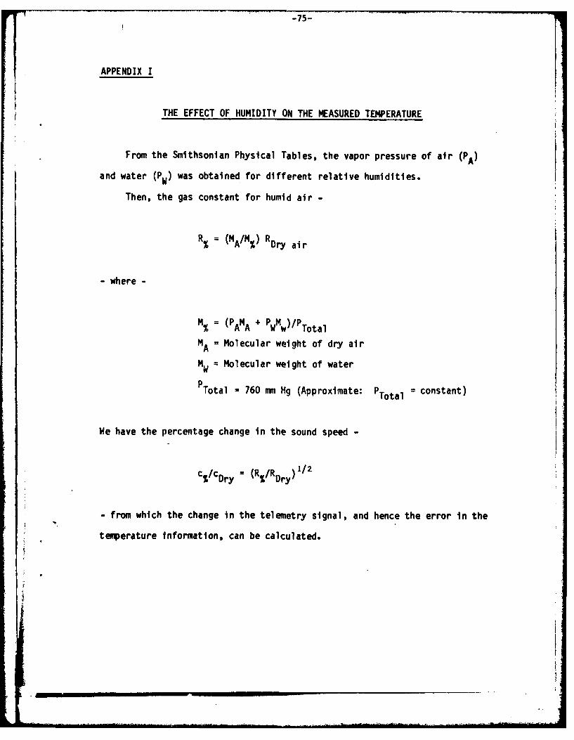
r7 -75-

APPENDIX I

THE EFFECT OF HUMIDITY ON THE MEASURED TEMPERATURE

From the Smithsonian Physical Tables, the vapor pressure of air (PA)

and water (Pw) was obtained for different relative humidities.

Then, the gas constant for humid air -

R = (MA/M%) RDry air

- where -

M% (PAMA + PwMw)/PTotal

M = Molecular weight of dry air

M = Molecular weight of water

PTotal = 760 mm Hg (Approximate: PTotal = constant)

We have the percentage change in the sound speed -

1/2c%/CDry = (R%/RDry)

- from which the change in the telemetry signal, and hence the error In the

temperature information, can be calculated.

-, b-

This gives -

T/ btent Humidity C%/Cdry AV# ATerror

300C 100% relative 1,0080 981Y 20C

200C 1,0045 72mV 1.4C

OOC 1,0011 130Y 0.25C

-500C 1,0000 0 0

(using &T/Av, - 0.2 °C/1lmV)

From the US Standard Atmosphere tables we have -

Tk m = -17.50C

Tlkm = - 56C

Thus, this effect is seen to be unimportant in the upper atmosphere.

It should, however, be kept in mind at low altitudes and on the ground.

-77-

Appendix 11

THE EFFECT OF VELOCITY FLUCTUATIONS ON THE MEASURED TEMPERATURE

The present design is intended for use as a balloon launched

instrument, and we must therefore take into consideration the velocities in

the soundpath that are associated with such operation.

The windspeed perpendicular to the soundpath, W, will arise from two

sources. During ascent or descent of the balloon it will consist mostly

of the rate of change of altitude. When the balloon is making measurement

at the pre-determined ' float-altitudes' it will be due to gusts in

the mean wind direction. Assuming an ascent rate of 6 m/s and a sound

speed of 295 m/s - the lowest sound speed in a flight to 25 km altitude,

which will give the largest relative error for a given wind speed - we find

that the contaminated temperature reading is some 0.10C below the true

temperature.

If we take 10% as a maximum turbulence level encountered by the

balloon and assume that the mean wind is not greater than 50 m/s (112 mph!)

we find that the effect of W while the balloon is floating is even less,

and hence we neglect it.

Splitting the wind velocity along the soundpath up into its mean and

fluctuating components - U = U + U' - we note that 17 will have no effect on

the measured temperature since the balloon is assumed to move with the mean

wind. However, U', the fluctuating part of the wind along the soundpath,

is of concern, as it will add'linearly to c in equation (11) in the text.

The gondola is spherical of roughly 12 feet diameter, and made of

aluminum tubing, with the transmitter and receiver positioned some 4 feet

away from it. Typical Reynolds numbers based on the gondola diameter will

be between one hundred thousand and one million depending on the gusts, and

the soundpath wil.l be in a mainly turbulent flowfield.

Also, the frame of the gondola will scatter the gusts and produce

additional turbulence.

The error in the temperature reading has been calculated, assuming

again 10% turbulent intensity. Some typical values are displayed -

U1~ O.U TApparent aTError

Away from gondola

-56.4°C(T ) lw/s 295 m/s -55.1 0C 1.30Cm Ps -52.0*C 4.40C

5 /s " -49.10C 7.30C

Towards gondola

N 1m, -57.9 0C -1.5oC

"/ -/s " -60.90C -4.40C-5/s -63.70C -7.30C

The Reynolds number quoted is based on the gondola diameter

(d 12 feet) -

Red .16 1107

d -" a 0- . -1 .

-79-

Appendix III

THE TEMPERATURE RANGE FOR VARIOUS CHOICES OF REFERENCE TEMPERATURE

AND PATH LENGTH

We will consider four different alternatives for pathlength and

reference temperature

(1)

Reference temperature T 0 25C = 298K0

Propagation velocity and wavelength at reference temperature

1/2

co = [yRT o = 346.4m/s

= co/f = 4.33 cm

where the signal frequency is constant f = 8000,0 Hz

Pathlength d = 2Ao = 8.66 cm

Te

rhus, at T=To the phase difference across the acoustic path Is zero.

-80-

The minimum temperature that can be measured unambiguously will cause

a phase difference of 180 degrees. That is, when-

d = (2 + 1/2)x

or

2orn = d = 3.46 cm

Thus, the minimum propagation velocity and temperature

cmin = mi; f = 277 mA

T m = 190.7K = - 82*C

ie - for this pathlength the dc-voltage output from the phase comparator

will decrease from it's maximum to its' minimum value as the air

temperature changes from plus 25 to minus 82 degrees centigrade. If the

temperature falls further the dc-voltage will increase again and cause

embi guity.

However, the digital phasemeter can measure over a full cycle (3600)

and would therefore give unambiguous readings down to -1410C.

In exactly the same manner we find

(2)Reference conditions T = 20°C = 293K0

co = 343.5 m/s

A° = 4.29 cm

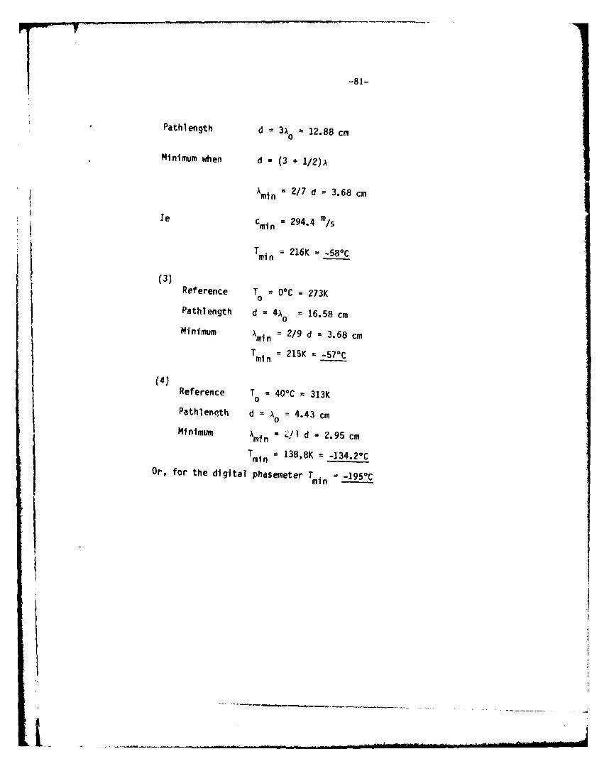
-81-

Pathlength d = 3x 0 12.88 cm

Minimum when d = (3 + 1/2)A

min = 2 /7 d = 3.68 cm

mmmle Cmi n =294.4 m/S

Tmin = 216K --580C

(3)Reference T = 0°C = 273K0

Pathlength d = 4x° = 16.58 cm

Minimum Amin = 2/ d = 3.68 cm

Tmi n = 215K -570C

Reference T = 400C - 313K0

Pathlenqth d = x = 4.43 cm0

Minimum Amin = :/ d = 2.95 cm

Tmi = 138,8K -134.2oC

Or, for the digital phasemeter Ti = .195c

IIi

[ ...... .... .. ...... ......... .........I

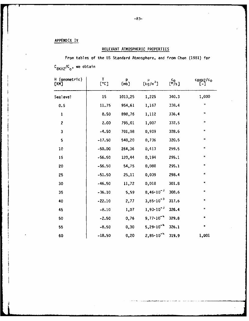
-83-

APPENDIX IV

RELEVANT ATMOSPHERIC PROPERTIES

From tables of the US Standard Atmosphere, and from Chen (1981) for

C 8KHZ /Co0, we obtain

H (geometric) T p P Oc8KHj/Co[KM] [0C] Emb] [kg/rn ] [mis]

Sealevel 15 1013,25 1,225 340.3 1,000

0.5 11.75 954,61 1,167 338.4 s

1 8.50 898,76 1,112 336.4

2 2.00 795,01 1,007 332.5 If

3 -4.50 701,08 0,909 328.6 i

5 1.0 540,20 0,736 320.5

10 -50.00 264,36 0,413 299.515 -56.50 120,44 0,194 295.1

20 -56.50 54,75 0,088 295.1s

25 -51.50 25,11 0,039 298.4

30 -46.50 11,72 0,018 301.8 I

35 -36.10 5,59 8,46-10- 308.6 s

40 -22.10 2,77 3,85-10- 317.6 o

45 -8.10 1,07 1,93-10 - 326.4

50 -2.50 0,76 9,77-10- 4 329.8

55 -8.50 0,30 5,29-10O' 326.1

60 -18.50 0,20 2,85-10-' 319.9 1,001

-85-

APPENDIX V

A DESCRIPTION OF A FEEDBACK SYSTEM USING A PHASE LOCKED LOOP INTEGRATED

CIRCUIT

Description of the Circuit

The closed loop circuit uses an XR-2212 phase locked loop Integrated

circuit whose VCO generates a squarewave signal of a frequency determined

by the phase and frequency of the input signals to the phase comparator.

This squarewave signal, after having been converted into a sine-wave is

amplified and used as the input signal to the transmitter.

After having been picked up by the microphone it is fed back through

the frequency analyzer as the input to the phase comparator. The reference

signal at the phase comparator is the squarewave generated by the VCO and

thus the phase difference measured by the phdse comparator is determined by

the phase lag of the acoust~c path (and across the various components

through which the signal passes).

The phase comparator produces an error voltage proportional to the

phase difference between its inputs

* d K cos at

-where Kd is the phase detector conversion gain and At the measured phase

difference.

This error voltage, after filtering, is the input to the VCO and hence

the frequency of the transmitted signal will depend on the phase difference

of the acoustic path. Thus changing the acoustic path will cause a change

in the transmitted signal in a direction that reduces the phase difference

between the transmitter and the microphone.

A simplified block diagram for the closed loop circuit, displaying its

operating principle, is given below.

-

4 - ---

7.L4 C~ 07'' -'c'j eS~ MOA1

, 'A-,c'.7r*.

The Performance of the Closed Loop

The lockrange of the phase-locked loop extends from about five to

eleven-and-a-half kilohertz.

Considering only the static response of the loop, we find that a

temperature fluctuation of 1 K will result in a frequency change of

between 4.5Hz and 15 Hz at different altitudes and for frequencies at the

two ends of the lock range.

-87-

Thus the closed loop does not appear to be as sensitive as the open

loop but the frequency change for a temperature change of 1 K is still

believed to be sufficient to obtain a temperature resolution of one degree

centigrade.

However, this analysis models the locked loop as a linear system and

is at best simplified. It does, for instance, not consider its stability.

For more information including circuit diagram and calculation of the

circuit parameters see AR 1044 of the Aerophysics Lab, MIT; from which we

quote the following conclusion--

the open loop, being a linear circuit as opposed to the non-

linear closed loop, is very much simpler to analyze and would thus appear

more suitable for the initial design efforts. It would also put less

stringent requirements on the acoustic properties of the transmitter and

experience none of the problems associated with loop stability.

-89-

APPENDIX VI

CIRCUIT DIAGRAMS AND SPECIFICATIONS FOR THE ELECTRONIC COMPONENTS

This appendix contains circuit diagrams and component listings for the

following electronic components (in the order listed).

Generator board

Filter board

Comparator board

Digital board

Regulator board

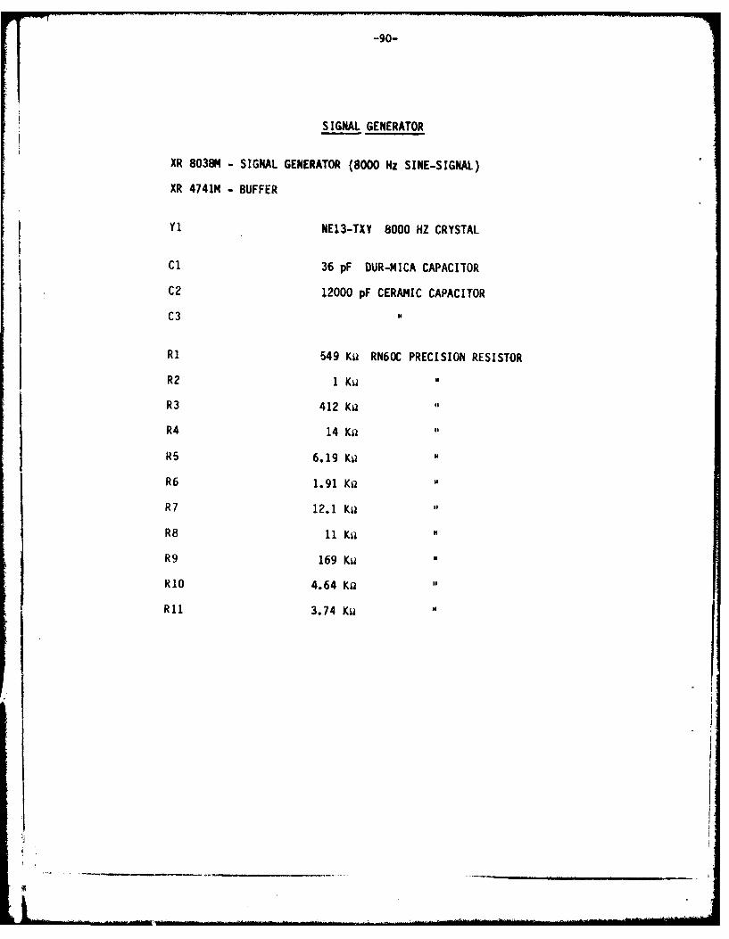
-90-

SIGNAL GENERATOR

XR 8038M - SIGNAL GENERATOR (8000 Hz SINE-SIGNAL)

XR 4741M4 - BUFFER

Y1 NE13-TXY 8000 HZ CRYSTAL

Cl 36 pF OUR-MICA CAPACITOR

C2 12000 pF CERAMIC CAPACITOR

C3a

Ri 549 Ka RN60C PRECISION RESISTOR

R2 1iKw u

R3 412 Ka 0

R4 14 Ka t

R5 6.19 Kw g

R6 1.91 Ka '

R7 12.1 Ka

R8 11 Kw

R9 169 Ku

R10 4.64 Ka

Rul 3.74 Ku N

.~U .-- -

8

a~~ Litl

0 cc

SE-

wA>I

+ MR.I~

0'

(D 00

cmTo

PO

0 m

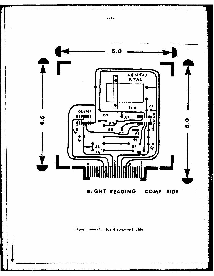
-92-

4*- 5.0

X44?41 0 : JCi

Is$ A IJ-'A

RIH EDN CO MP SIDSial ge a a r i0 II..h.'.uEh....~LEJ/s-*J ,

fn i

if _

-93-

@0

Ililil11li l 11II 1lIGROUND SIDE

Signal generator board ground side

-94-

FILTER

XR 4741 BUFFER

LM 101 FILTER OP AMP

Cl 2000 pF DUR-MICA CAPACITOR

C2 5 pF

C3 [Removed]

C4 1 UF CERAMIC CAPACITOR

Ri 3.91 Ka RN60C PRECISION RESISTOR

R2 6.01 K9

R3 9.96 Kil

R4 1.5 Mu

R5 1.5 No

R6 9.97 Ka

R7 4.49 Ku

R8 1.5 Mu

R9 9.98 Kw

RIO 100. 4 a

RII 301 Ks4

R12 IKit

R13 9.09 Ka

R14 82.5 Kia

R15 200 Ka

R16 1.5 Mu

(NJ

LL * L.

- *-

LL *u- tLa

a:0,4-

-NOI- - -

00

C- - 2

100crI

xa - U

U a: U) -

T JC)U

a , II

et

COMIP SIDEr

Efd

Eight khz b~ndpass filter board component s'ide

-97-

GROUN SIDE0

Eih kh0adasfle or gon side

.lose .--.-. logo- - -. ,-- less-- 0

-98-

COMPARATOR

LM 311/111 MOTOROLA VOLTAGE COMPARATOR MILSPEC

XR 2208 M EXAR PHASE COMPARATOR

MC 14040 B MOTOROLA 12 BIT COUNTER

XR 4741 M EXAR OP AMP

Ri 4.99 Ku RN 60C R17 10 Ka RN 60C

R2 4.99 Ku " Ri8 10 Ku "

R3 1 Ki " R19 2 Ka

R4 [REMOVED] R20 2 Kai

R5 3.01 K " R21 2 Ka

R6 2 Ki " R22 100 Ku RN 65 D

R7 1.5 Mu

R8 1.5 Mii Cl 330 pF DUR-MICA CAP.

R9 1.5 Ms2 22000 pF CERAMIC CAP.

RIO 1.5 M2 " C3 22000 pF

R11 1.5 Mu " C4 10 pF

R12 1KQ " C5 2200 pF

R13 2 Ku " C6 I PF

R14 1 Ku " C7 12000 VF "

R15 3.92 Xa " C8 I lF"

RIb 10 K

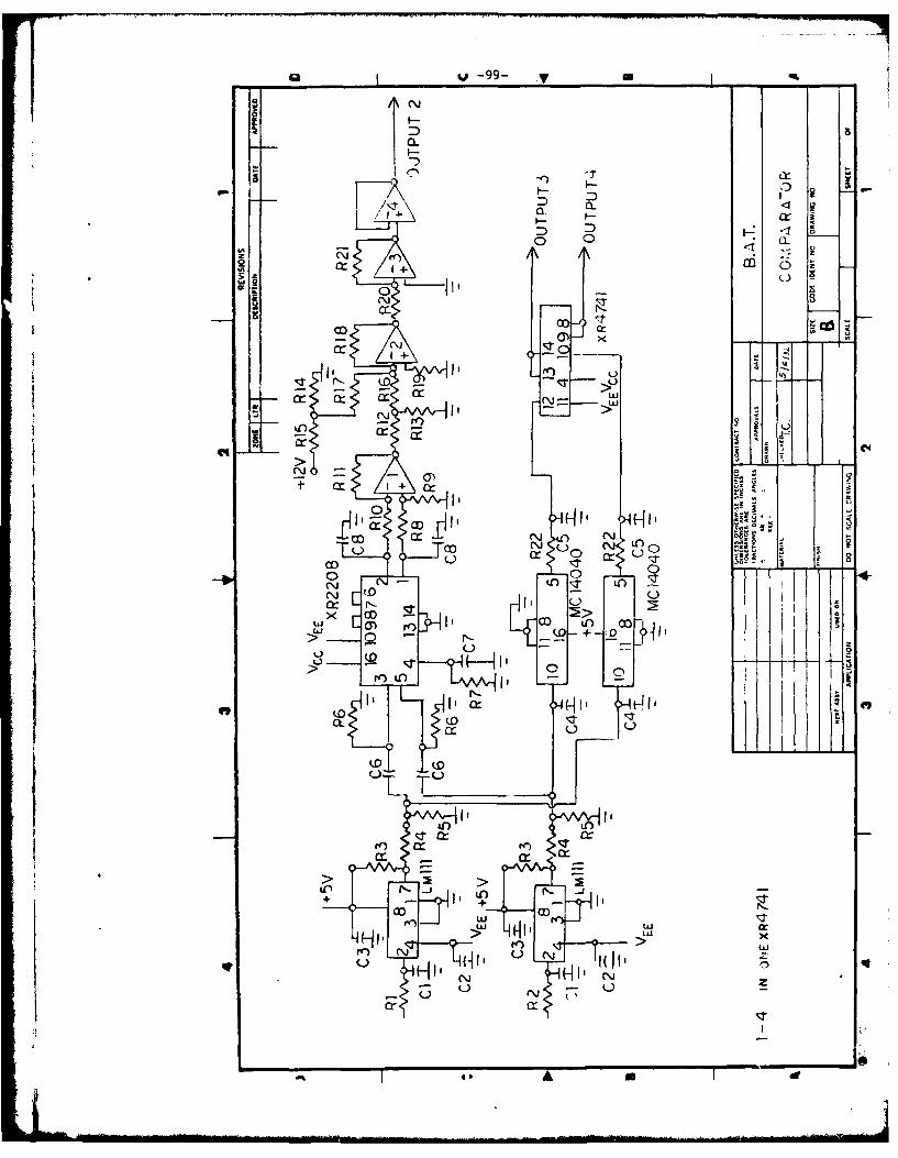
w u- 9 9 - -T m

a.9-. HI

c'Ja. l-~ C 0

94-4

0 Ii' C>co C

'o '

(D - LU _

L) (D

(\J------4(D r -

0 cc

(D N f) c 0

u .

(%4Dt0: c0c .4

coJ CM

010

x

T toWz

C~j C~jA V

I AD-A1i1 774 MASSACHUSETTS INST OF TECH CAMBRIDGE AEROPHYSICS LAB F/6 20/1

DEVELOPMENT OF AN AIRBORNE SONIC THERMOMETER. (U)SEP 82 T R CHRISTIANSEN F19628-80-K-0089

UNCLASSIFIED AFGL-TR-82-119 NLSaflllllflllfll

INNhNlNNNNlk

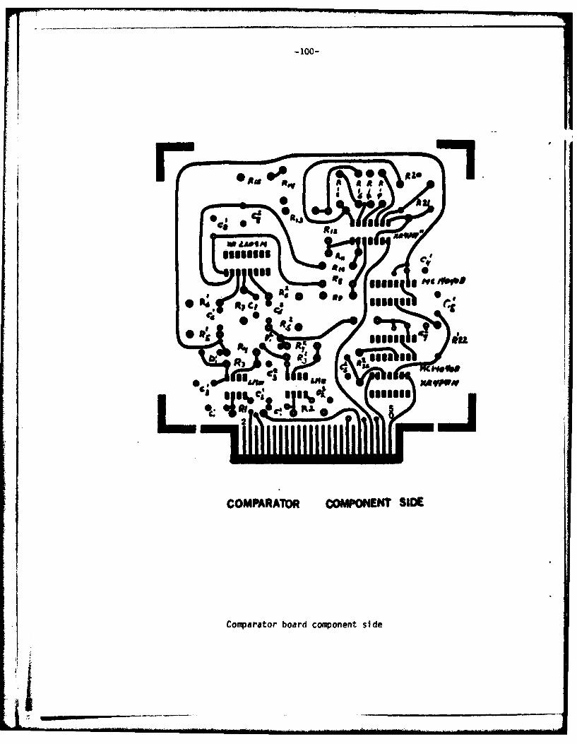
-100-

it' Row It A

A o;it ato, bor cornn sde s

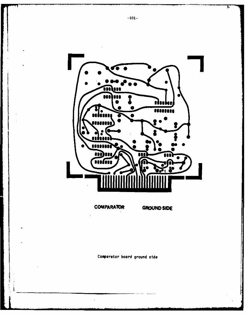
oi Is

COMARTO seeN SD

Coprtrbar rudsd

DIGITAL PHiASEMETER

MC 14011 B MOTOROLA QUAD 2-INPUT NANO-GATE

MC 14013 B NDUAL TYPE D FLIP-FLOP

MC 14040 B 12 BIT BINARY COUNTER

MC 14042 8BS QUAD LATCH

MC 14049 B8S HEX BUFFER

MC 14521 B 24 STAGE FREQUENCY DIVIDER

MC 14521 B DUAL COMPLEMENTARY PAIR PLUS INVERTER

8 MHz CRYSTAL

R1 3.3 Ka CARBON RESISTOR 6%

C1 330 pF OUR-MICA CAPACITOR

C2 330 pF

(Miscellaneous capacitors from V c and V EE to ground)

K~~ ~~~~~ ~~~ ._____________ .___. __.__.....___

-103-

+vM10C 1 MC 1K140138 IM 314-4042B (U JI

4011P2 129

14040 +5V _y

;'D S2402WA '1

0 -j( 27

IV Mc14013 ~ ~ BA 12042831

6~ (74IR2 02

1 4 102* CCD NNEC E

Diia paemee chmtc iga

-104-

uso

Mel I fof ie

ConPONU?4F 3106

Digital phase meter board component side

-105-

" 1 .....IN,,,M

r0

Dtgttal~~ ~ AILs mete or rudsd

.. .. .. . . Il i, = / - I ": . . .. l -

: " : . . . . .

-106-

REGULATOR

MC 7824 + 24 V REGULATOR

MC 7812 + 12 V

MC 7805 + 5V "

MC 7924 - 24 V

MC 7912 - 12 V

Cl 1 AF CERAMIC CAPACITOR

Dl 1N91 DIODE

RI 220 i - 470 u RN 60C PRECISION RESISTOR

LEOI LIGHT EMITTING DIODE

.,t-. -- --.- __I_ _ -__I

II

ILI

U'0

Fli +I-

- 'a j

5i >i

Of :

CD co o cm

(uJ CN50'n f-f'+)t\

-108-

0 0

00

*0 C0L 0

REGLATOR COMPONT SID

Voltage regulator board component side

-109-

0O

0S.

0 00

0

REGULATOR GROUND SIDE

Voltage regulator board ground side

-111-

Appendix VII

SPECIFICATIONS FOR THE ACOUSTIC COMPONENTS

This appendix contains information about the following acoustic

components --

The electrostatic transmitter

The condenser microphone and preamplifier.

For more complete technical Information about the microphone,

pre-amplifier and supply see AR 1042 of the Aerophysics Lab and technical

literature from Bruel and Kjaer.

ELECTROMAGNET7IC TRANSMITTERSCL

ALUMINUM SPIRALMYLARi DIAPHRAGM

-I C 3OLTR IN (S A N D SQCR LW

~29 1NAY AR OPRWR

HOLES FOR PRESSUREEQUAL ISAT ION

~~44

T/16

?'CAA

kEW~ FOR -YL - -

A TIAC iIIN~i DIAPHRAMTfANSMIT Ttf,' T@

-

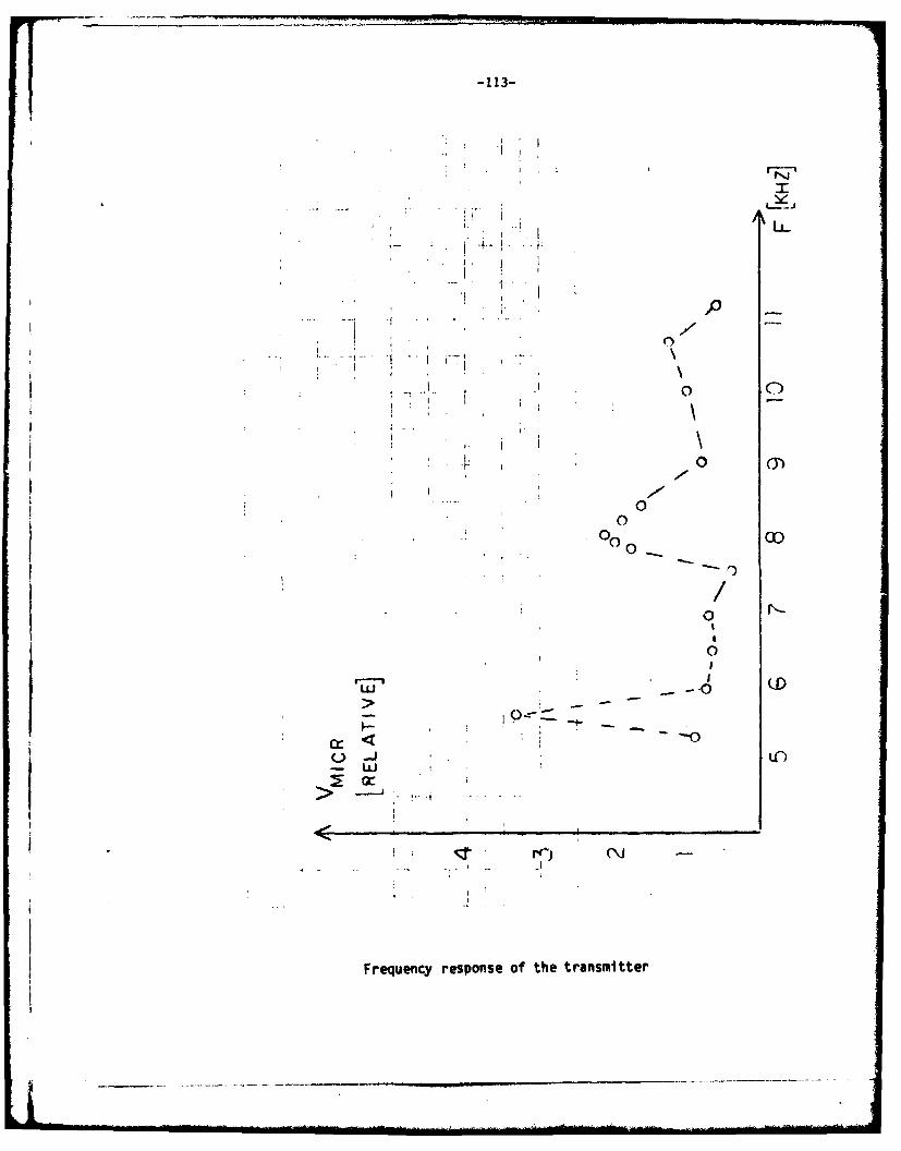
-113-

C7

I0 C)

0 f-

-0

Frequency ~ ~ ~ repneoftetanmte

**)/

co-

/

0

wP

, -

J Frequency response of the transmitter

-"14-

SPECIFICATIONS FOR THE ALUMINIZED 1MYLAR -

products2909 East 79th Street, Cleveland. Ohio 44104 * Area Code 216 Phone: 883-8484 .Telex: 980-591

LAMOTAPE 951 TENTATIVE PRODUCT DATA SHEET

Description: Electrical Shielding Tape

Construction: .00092" Polyester Film.001" Aluminum Foil

951 Physical Data

Finished Weight: 3.04 oz./SY f 5%

Specific Gravity: 2.028

Breaking Strength: 28 lbs. per inch width

Tensile Strength: 14,000 p.s.i.

Elongation at Break: 100%

Gauge: 0.0020 t 5%

Color: Natural - Aluminum

Weight: 1,000 ft., 1" wide - 1.76 lbs.

Yield: 5.3 square yards per lb.

s. -115-

ITHE CONDENSER MICROPHONE

Some tmportant data -

! .11 .0

JI:'1 " I II !1I- IIII0

Le

114146

lowp~

a. ITs46 46

I I

m~l so mi I Ik 6 3 f Y o o

so s 70 100 20

Powiatei ehg

Fig. 6.44. Sensitivity variation of half-inch microphones Types 4165and 4166 at 250 Hr *as a function of polarization voltage

-41Tye 16

PI Pe 416

-117-

-ni -- 9 1 s

Fi. 6.5 7. Effect of low Pressure on frequency response of half-inch microphone

Type 4165Note that 760 mmr HV 1 1~3 mbarI arm,

'14-I-4- IM 1 111

-4

Fig.6.62. Variatio of aeSWIh*t ot 250H.- with ambient static pes.SAM 1Wr h lich microphones Type 45

APPENDIX VIII

A POSSIBLE MODEL FOR PREDICTING THE EFFECT OF RADIATION HEATING IN THE

ATMOSPHERE

The following estimate is based on numerical values given by Lichfield

& Carlson (1967) for solar input and blackbody radiation.

Approximate surface area of chassis box: Top 0.16 m2

Bottom

Short sides 2 x 0.06 m

Long sides 2 x 0.07 m

Total .58 m

Assume roughly one fifth of the chassis box is exposed to the sun

A ex.~0.1 m 2

exp.

The power radiated in will be due to direct solar - and to infrared -

radiation.

2A typical solar input at float is 1200 w/m . Hence -

Power received from solar radiation - 120 W

A typical value for infrared radiation is given as 128 W/m2 and hence,

if assuming that the whole chassis box receives this, we have -

........ __.... . ................ . I________.. . ... ___-_....._____-__

Power received from infrared radiation 65W

Thus, the total power input at float is 185 Watts.

The surface temperature is at equilibrium when the incoming energy

equals the outgoing energy. The relationship between radiated power and

temperature is -

E a ekT

- where e is the emissivity, a characteristic of the radiating surface and

k is the Stefan-Boltzmann constant.

For a blackbody, where e is one, the outside surface temperature

obtained from this power input would be about -30*C. For the aluminum

chassisbox the exact emissivity would probably be about 0.1 thus lowering

the surface temperature.

Assume for this simplified analysis that the chassisbox has no thermal

resistance, but is covered by insulation with surface characteristics like

a black body.

If the minimum tolerable temperature inside the chassisbox is +50C

the temperature difference across the insulation must be at least 35*C.

Since we have very low densities in the high atmosphere we ignore

heat transfer by convection. Assuming pure conduction, with a linear

temperature distribution, the heat transfer across the insulation Is given

by-

IL

q - k dT/dx

a (k/h)insulation (Tinside- Toutside)

- where h is the thickness of the insulation.

Now, the amount of heat we need to conduct out of the chassisbox is

that dissipated in the electronic circuitry, given by

d = I vj -I iI

The total amount of power drawn by the instrument is approximately 27

watts but out of this some 13 watts is dissipated in conducting spiral of

the transmitter. Thus the power dissipated in the box is about 14 watts.

Assuming that this power is conducted out evenly by the total box sur-

face gives the heat transfer as 24 W/m. Note that the assumption

of even distribution of heat transfer is unrealistic since it would require

mixing of the air inside of the box by convection; but that we will use it

here in lack of any better prediction.

Thus if we assume an Insulation thickness of 2 cm's we get the

following requirement to its' condutivity -

k ins (4,)h

* (j v I jl/AT)h

- 1.4 1 101 W/m°C

-12 1-

This is about one tenth of the conductivity of the chassis box, and

thus shows that insulation is necessary.

Although this analysis contains the theoretical framework for finding

the necessary requirements of the insulation, it involves too many

'guesstimates' to yield meaningful information at present (eg - percentage

of the chassisbox exposed to sunlight, emissisivity of the insulation,

thermal resistance and heat transfer distribution in the chassisbox, etc.).

For the first launch time does not permit a closer analysis, so it was

decided to insulate moderately and measure the temperature in the chassis

box throughout the flight. However, the problems associated with

controlling the temperature of the instrument should be carefully

considered in the future.

OI

-123-

APPENDIX IX

A THEORETICAL CALIBRATION CJRVE

Equation 20 gives, with To - 25*C

T(C] Vs[Volta] T['C] VS[Volts] TICI VS[Volts]

29 0.009 9 0.161 -11 0.864

28 0.005 8 0.182 -12 0.914

27 0.002 7 0.205 -13 0.966

26 0.001 6 0.229 -14 1.019

25 0.000 5 0.255 -15 1.073

24 0.001 4 0.282 -16 1.129

23 0.002 3 0.311 -17 1.186

22 0.005 2 0.341 -18 1.244

21 0.010 1 0.372 -19 1.304

20 0.015 0 0.405 -20 1.365

19 0.022 -1 0.440 -21 1.427

18 0.030 -2 0.475 -22 1.491

17 0.039 -3 0.513 -23 1.555

16 0.049 -4 0.552 -24 1.621

15 0.061 -5 0.592 -25 1.688

14 0.074 -6 0.633 -26 1.756

13 0.089 -7 0.677 -27 1.825

12 0.105 -8 0.721 -28 1.894

11 0.122 -9 0.767 -29 1.965

10 0.141 -10 0.815 -30 2.037

-124-

T[°CI vo1volts] T['C) va[volts] T[°C) vo[voltsl

-31 2.110 -49 3.489 -67 4.660

-32 2.183 -50 3.565 -68 4.706

-33 2.257 -51 3.640 -69 4.749

-34 2.332 -52 3.715 -70 4.789

-35 2.407 -53 3.788 -71 4.826

-36 2.483 -54 3.861 -72 4.860

-37 2.560 -55 3.932 -73 4.890

-38 2.637 -56 4.003 -74 4.918

-39 2.714 -57 4.071 -75 4.941

-40 2.791 -58 4.139 -76 4.961

-41 2.869 -59 4.205 -77 4.976

-42 2.947 -60 4.269 -78 4.988

-43 3.025 -61 4.331 -79 .996

-44 3.103 -62 4.391 -80 5.000

-45 3.181 -63 4.450 -81 4.999

-46 3.259 -64 4.506 -82 4.994

-47 3.336 -65 4.560 -83 4.984

-48 3.413 -66 4.611 -84 4.970

I __ ____ ____