Actuator Networks for Navigating an Unmonitored Mobile Robot

Jeremy Schiff§, Anand Kulkarni†, Danny Bazo§, Vincent Duindam§,Ron Alterovitz§, Dezhen Song‡, Ken Goldberg§†

§ Dept. of Electrical Engineering and Computer Sciences, University of California, Berkeley, CA 94720-1770, USA† Dept. of Industrial Engineering and Operations Research, University of California, Berkeley, CA 94720-1777, USA

‡ Dept. of Computer Science, Texas A&M University, College Station, TX, 77843-3112, USA{jschiff|anandk|dbazo|vincentd|ronalt|goldberg}@berkeley.edu, dzsong@cs.tamu.edu

Abstract— Building on recent work in sensor-actuator net-works and distributed manipulation, we consider the use ofpure actuator networks for localization-free robotic navigation.We show how an actuator network can be used to guide anunobserved robot to a desired location in space and introducean algorithm to calculate optimal actuation patterns for such anetwork. Sets of actuators are sequentially activated to inducea series of static potential fields that robustly drive the robotfrom a start to an end location under movement uncertainty.Our algorithm constructs a roadmap with probability-weightededges based on motion uncertainty models and identifies anactuation pattern that maximizes the probability of successfullyguiding the robot to its goal.

Simulations of the algorithm show that an actuator networkcan robustly guide robots with various uncertainty modelsthrough a two-dimensional space. We experiment with additiveGaussian Cartesian motion uncertainty models and additiveGaussian polar models. Motion randomly chosen destinationswithin the convex hull of a 10-actuator network succeeds withwith up to 93.4% probability. For n actuators, and m samplesper transition edge in our roadmap, our runtime is O(mn6).

Keywords: Sensor Networks, Actuator Networks, RoboticNavigation, Potential Fields, Motion Planning

I. INTRODUCTION

As robots become smaller and simpler and are deployed inincreasingly inaccessible environments, we need techniquesfor accurately guiding robots in the absence of localization byexternal observation. We explore the problem of observation-and localization-free guidance in the context of actuatornetworks, distributed networks of active beacons that imposeguiding forces on an unobserved robot.

In contrast to sensor networks, which passively observetheir environment, actuator networks actively induce a phys-ical effect that influences the movement of mobile elementswithin their environment. Examples include light beaconsguiding a robot with an omni-directional camera through thedark, electric fields moving a charged nano-robot througha fluid within a biological system, and radio transmitterson sensor motes guiding a robot with a single receiver.

*This research is supported in part by NSF CISE Award: Collabo-rative Observatories for Natural Environments (Goldberg 0535218, Song0534848), Netherlands Organization for Scientific Research (NWO), NIH(F32CA124138), by NSF Science and Technology Center: TRUST, Team forResearch in Ubiquitous Secure Technologies, with additional support fromCisco, HP, IBM, Intel, Microsoft, Symmantec, Telecom Italia and UnitedTechnologies, and by the AFOSR Human Centric Design Environmentsfor Command and Control Systems: The C2 Wind Tunnel, under thePartnership for Research Excellence and Transitions (PRET) in HumanSystems Interaction.

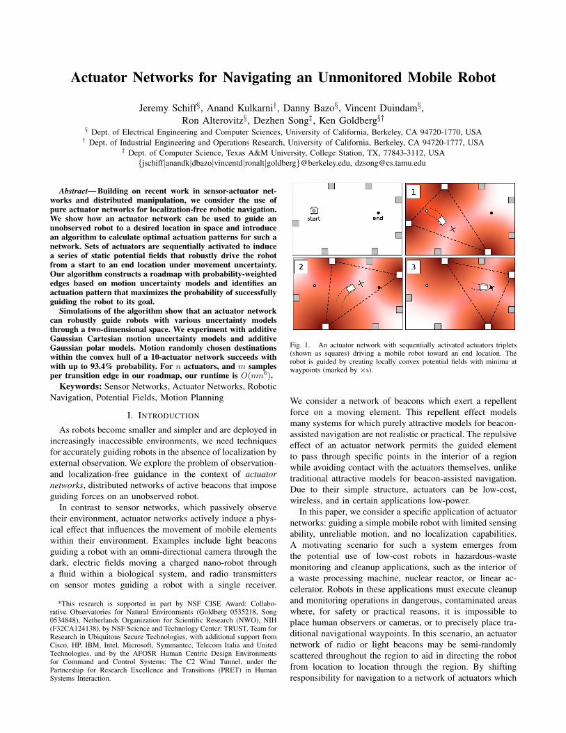
Fig. 1. An actuator network with sequentially activated actuators triplets(shown as squares) driving a mobile robot toward an end location. Therobot is guided by creating locally convex potential fields with minima atwaypoints (marked by ×s).

We consider a network of beacons which exert a repellentforce on a moving element. This repellent effect modelsmany systems for which purely attractive models for beacon-assisted navigation are not realistic or practical. The repulsiveeffect of an actuator network permits the guided elementto pass through specific points in the interior of a regionwhile avoiding contact with the actuators themselves, unliketraditional attractive models for beacon-assisted navigation.Due to their simple structure, actuators can be low-cost,wireless, and in certain applications low-power.

In this paper, we consider a specific application of actuatornetworks: guiding a simple mobile robot with limited sensingability, unreliable motion, and no localization capabilities.A motivating scenario for such a system emerges fromthe potential use of low-cost robots in hazardous-wastemonitoring and cleanup applications, such as the interior ofa waste processing machine, nuclear reactor, or linear ac-celerator. Robots in these applications must execute cleanupand monitoring operations in dangerous, contaminated areaswhere, for safety or practical reasons, it is impossible toplace human observers or cameras, or to precisely place tra-ditional navigational waypoints. In this scenario, an actuatornetwork of radio or light beacons may be semi-randomlyscattered throughout the region to aid in directing the robotfrom location to location through the region. By shiftingresponsibility for navigation to a network of actuators which

directs a passive robot, smaller and more cost-effective robotsmay be used in these applications.

We consider the 2D case, where the actuator networkconsists of beacons at different locations in a planar environ-ment. The actuator network is managed by control softwarethat does not know the position of the robot, but it is awareof the positions of all of the actuators. Such software maybe either external to the system, or distributed across theactuators themselves, as in the case of a sensor network.We assume only that the robot’s sensor is able to detectand respond consistently to the strength and direction ofeach actuation signal. Such a general framework accuratelyrepresents a wide variety of real-world systems in use todayinvolving deployed navigational beacons, while significantlyreducing the technical requirements for both the beacons andthe robots.

We present an algorithm that sequentially switches be-tween sets of actuators to guide a robot through a planarworkspace towards an end location as shown in Figure 1.Using three non-collinear actuators, each one generating arepellent force field with intensity falling off inversely pro-portional to the square of the distance, we generate potentialfields that drive the robot from any position within the convexhull of the actuators to a specific position within the interiorof the triangle formed by the actuators (the local minimum ofthe potential field). The optimal sequence of potential fieldsto move the robot to a specific point within the interior of theworkspace is determined using a roadmap that incorporatesthe possible potential fields as well as uncertainty in thetransition model of the robot. Despite this uncertainty and theabsence of position measurement, the locally convex natureof potential fields ensures that the robot stays on track. Wepresent results from simulated actuator networks of smallnumbers of beacons in which a robot is successfully guidedbetween randomly chosen locations under varying modelsof motion uncertainty. With as few as 10 actuators in arandomly-placed actuator network, our algorithm is able tosteer a robot between two randomly selected positions withprobability 93.4% under motion uncertainty of 0.2% standarddeviation Gaussian Polar motion uncertainty (perturbing therobot’s magnitude and angle with additive Gaussian motionuncertainty).

II. RELATED WORK

There is a long history of investigation into the charac-teristics of potential fields induced by physical phenomenaand how objects are affected by these fields. Some of theearliest work, related to the study of gravitational, electricand magnetic fields, as well as topological properties of suchfields, was pioneered by Newton, Gauss, Laplace, Lagrange,Faraday, and Maxwell [1], [2].

Potential functions for robotic navigation have been stud-ied extensively as tools for determining a virtual field which arobotic element can follow to an end location while avoidingobstacles. See Choset et al. [3] for an in-depth discussion.Khatib proposed a model where an end location is repre-sented as an attractor, obstacles are represented as repulsers,

and the overall field is determined by the superposition ofthese fields [4], [5]. While these fields are typically referredto as potential fields, they are actually treated as vector fieldsthat provide the desired velocity vector for the robot at anylocation in space. While moving, the robot performs simplegradient descent on this space. Motion planning requiresdefining attractive and repulsive fields such that the robotwill always settle at a local minimum created at the endlocation. Several extensions exist to this classical approach,for example to prevent the robot from getting stuck at a localminimum [6] and to deal with moving obstacles [7], [5].

Rimon and Koditschek addressed this problem by deter-mining the attractive and repulsive potential functions neces-sary to guarantee unique minima [8]. They accomplished thisby defining functions over a “sphere world” where the entirespace and all obstacles were restricted to be n-dimensionalspheres. They discovered a mapping from this solution toother types of worlds such as “star-shaped worlds”, allowingfor a general solution to this problem. Connolly et al. [6] useharmonic functions in the repulsive and attractive functionsto avoid local minima. In our work, we also address theproblem of local minima, but are restricted in our choice ofpotential functions.

Whereas past research has treated modeling a robot’senvironment and guidance instructions as an arbitrary virtualpotential function, our work considers a network of actuatorswhich emit signals from given, fixed positions and explicitlymodels physical phenomena. In our formulation, these actu-ators are the sole contributors to the potential field, ratherthan the environment or guidance information. In addition,the potential fields in our algorithm transition at discrete timesteps, and problems related to local minima are avoided bysteering the robot through waypoints, rather than directlyfrom start to end location.

The concept of distributed actuation has been studied invarious contexts. Li et al. [9] examined how to directlyapply potential functions in a distributed fashion over sen-sor networks, focusing on formulating the algorithm in adistributed manner. Pimenta et al. [10] addressed the robotnavigation problem by defining force vectors at the nodes ofa graph. They assume, however, that nodes can be arbitrarilyadded to the graph, contrary to our problem formulation inwhich the actuators are provided as input and are fixed.Finally, research in distributed manipulation has examinedhow to leverage many actuators to perform coordinatedmanipulation, focusing primarily on the use of vibratoryfields to place and orient parts [11], [12], [13], [14], [15].

To actively construct potential fields to steer a mobile robotsubject to uncertainty in motion and sensing, we build onprevious results in motion planning under uncertainty [16].Motion planners using grid-based numerical methods and ge-ometric analysis have been applied to robots with motion andsensing uncertainty using cost-based objectives and worst-case analysis [17], [18], [16]. Markov Decision Processeshave been applied to motion planning with uncertainty inmotion, but these methods generally require state sensingand are not directly applicable to actuator networks [19],

[20], [21], [16].In this paper, we consider a hybrid sensing uncertainty

model: the actuator network cannot sense the mobile robotbut the mobile robot can sense the potential field. Lazanasand Latombe proposed a landmark-based approach in whichthe robot has improved sensing and actuation inside land-mark regions, reducing the complexity of the motion plan-ning problem to moving between these regions [22]. Anactuator in an actuator network can be viewed as a gen-eralization of a landmark that can be controlled and canexert influence over the mobile robot at arbitrary distances.As with sensing uncertainty, this paper considers a hybridactuation uncertainty model: the actuator network generatesa precise potential field with no uncertainty while the mobilerobot is subject to uncertainty in its motion. To addressmotion uncertainty, Alterovitz et al. introduced the StochasticMotion Roadmap (SMR), a sampling-based method thatexplicitly considers models of motion uncertainty to computeactions that maximize the probability that a robot will reachan end location [21]. As in SMR, we use the objectiveof maximizing probability of success over a roadmap. Butunlike SMR, which assumes perfect sensing, the maximumprobability path for an actuator network must be computedbefore plan execution is begun since sensing feedback is notavailable.

III. PROBLEM FORMULATION

A. Assumptions

We consider the control of a single mobile robot in aplanar environment, influenced by an actuator network. Then actuators are located at known positions xi ∈ R2. Eachactuator can be controlled independently to produce a signalwith piece-wise constant amplitude ai(t) ≥ 0. Each actuatorgenerates a radially symmetric potential field Ui of the form

Ui(x) =ai

|x− xi|(1)

The direction and magnitude of the gradient of this field canbe observed from any location x ∈ R2 and are given by thevector field Fi

Fi(x) =∂Ui

∂x= −ai(x− xi)

|x− xi|3(2)

i.e. the signal strength |Fi(x)| is inversely proportional tothe square of the distance to the actuator, as is common forphysical signals.

The aim of the actuator network is to guide a mobilerobot along the direction of steepest descent of the combinedpotential field U(x) =

∑i Ui(x). The position of the robot

as a function of time is denoted by p(t) ∈ R2, and the robotis assumed to have sufficient local control to be able to moveapproximately in a given direction vector v (relative to itsown coordinate frame). The desired motion direction v isequal to the direction of steepest descent of the combinedpotential field U and is hence given by the vector sum

v = −∑

i

Fi(x) =∑

i

ai(x− xi)|x− xi|3

(3)

Under this control strategy, each of the actuators serveseffectively as a “robot repulser”, causing the robot’s directionof motion to be determined by the total combined force fromall actuators. We only assume that the robot can continuouslymeasure the direction and strength of the superimposedactuator signals. In particular, no global position sensors orodometry is required. Its motion is described by a generalmodel p = R(v), which may include stochastic componentsto represent sensor and actuator uncertainty, or general un-certainty in movement across the workspace due to viscosityin a fluid environment, uneven terrain causing wheel slip, orsimply unreliability in the robot’s design.

The design of a suitable sensor for the robot to measurethe actuator signals depends on the type of actuation used.For light-based actuation, one could use an omni-directionalcamera. Each actuator signal from a certain direction causesa specific spot in the image to light up with a brightnessdepending on the actuator strength and distance. The desiredmotion vector v can then be computed simply by adding theforce directions corresponding to all image pixels, weightedby their brightness.

A centralized controller is assumed to know the location ofthe actuators and to be able to control the actuator amplitudesin a time-discrete manner. It does not have other sensinginformation; in particular, it cannot measure the robot’sposition.

B. Inputs and Output

The inputs of the control algorithm are the initial locationp0 = p(0) ∈ R2, the end location pe ∈ R2 of the robot, andthe locations of each actuator xi ∈ R2. The actuator locationscan either be determined a priori, or via some localizationscheme. The key aspect is that the actuators will not observeor track the robot.

The proposed algorithm returns a sequence of actuatoramplitudes {ai(tj)} at discrete time instants tj that maxi-mizes the probability that the robot successfully moves fromthe start location p0 to the end location pe. If no pathfrom p0 to pe can be found, the algorithm returns theempty sequence. Each set of amplitudes contains exactlythree nonzero values corresponding to a particular triangleof actuators and an associated start and destination location.The use of only three actuators at a time has the advantageof simplifying the analysis of the system and potentiallyreducing power consumption of the network by limiting thenumber of active actuators at any time. To conserve power,all idle actuators can go into a low-power state. Each timeinstance is separated by a sufficiently large duration that arobot starting at the associated start location will by this timeeither have migrated to the associated target location movingat minimum velocity or will be outside the actuator triangleand get progressively farther away. This time is determinedby the minimum speed of the robot.

C. Motion Uncertainty

To investigate the utility of actuator networks in steeringrobots with uncertain motion, we considered two uncertainty

models R(v): one using additive random Gaussian noise onthe robot’s Cartesian coordinates, and one using additiverandom Gaussian noise on the robot’s polar coordinates.In other words, the Cartesian motion uncertainty modeldescribes the uncertain motion of the robot as[

px

py

]= p = R(v) =

[N(vx, σ

2)

N(vy, σ

2)] (4)

while the polar motion uncertainty model is given by[px

py

]= p = R(v) =

[r cos(θ)r sin(θ)

](5)

where r and θ are drawn from Gaussian distributions as

r = N(|v|, σ2

)θ = N

(atan2(vy, vx),

σ2

4π2

)IV. MOTION CONTROL USING ACTUATOR NETWORKS

To solve the problem of finding a valid actuation sequence(if one exists), the algorithm first generates all possible

(n3

)triangles that can be formed using the n actuators. Then,it computes the incenters of these triangles (as discussed inSection IV-A) to be used as local minima of the potentialfields. These incenters define the vertices in a graph, and thenext step of the algorithm is to determine the weights of allpossible edges between the vertices. We define the weightof an edge to be the probability that the robot successfullynavigates from one vertex to the other, as defined by the robotmotion model R(v). The resulting graph defines a roadmapfor the robot, and the last step of the algorithm is to insertthe start and end locations into the roadmap and determinethe path between them that maximizes the probability ofsuccessfully reaching the end location.

A. Local control using actuators triplets

The following assumes the actuators we choose are notcollinear. Consider a potential field U generated by anactuators triplet i, j, and k (and all the other actuators inthe network set to zero amplitude). If the amplitudes of theactuator triplet is strictly positive, the potential field willhave a local minimum at some point inside the triangle.This location is called the waypoint of the potential field.In our global algorithm, we may traverse many waypoints toget from the start to the end location. The final waypoint isdefined to be the end location. For a given triangle structure,we define the feasible region as the set of locations that canbe made waypoints, that is, local minima of the potentialfield. The feasible region is clearly strictly smaller than thetriangle defined by the active actuators.

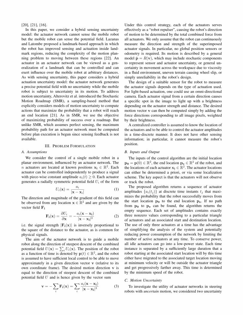
For a given waypoint x, C(x) is the capture region of awaypoint as the set of all points x ∈ R2 such that, whenfollowing the direction of steepest descent from x, one willeventually arrive at x. Some examples of capture regions forvarious triangles and waypoints are given in Figure 2.

For a point x to be a local minimum of the potential field,the gradient ∂U

∂x at x should be zero, and the Hessian matrix

Fig. 2. Examples of two different triangles and three different waypoints(denoted as circles) and their capture regions (shaded areas) for bothtriangles. The incenter of each triangle is marked with a ’+’.

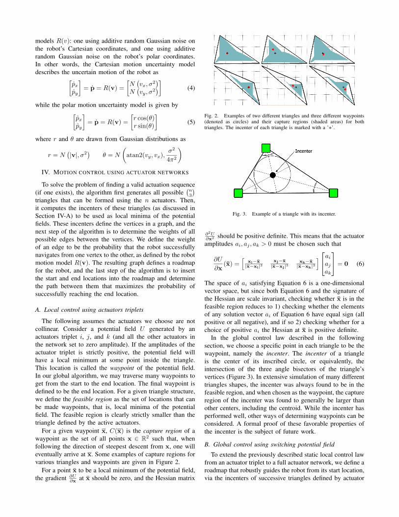
Fig. 3. Example of a triangle with its incenter.

∂2U∂x2 should be positive definite. This means that the actuatoramplitudes ai, aj , ak > 0 must be chosen such that

∂U

∂x(x) =

[xi−x|x−xi|3

xj−x|x−xj|3

xk−x|x−xk|3

]ai

aj

ak

= 0 (6)

The space of ai satisfying Equation 6 is a one-dimensionalvector space, but since both Equation 6 and the signature ofthe Hessian are scale invariant, checking whether x is in thefeasible region reduces to 1) checking whether the elementsof any solution vector ai of Equation 6 have equal sign (allpositive or all negative), and if so 2) checking whether for achoice of positive ai the Hessian at x is positive definite.

In the global control law described in the followingsection, we choose a specific point in each triangle to be thewaypoint, namely the incenter. The incenter of a triangleis the center of its inscribed circle, or equivalently, theintersection of the three angle bisectors of the triangle’svertices (Figure 3). In extensive simulation of many differenttriangles shapes, the incenter was always found to be in thefeasible region, and when chosen as the waypoint, the captureregion of the incenter was found to generally be larger thanother centers, including the centroid. While the incenter hasperformed well, other ways of determining waypoints can beconsidered. A formal proof of these favorable properties ofthe incenter is the subject of future work.

B. Global control using switching potential field

To extend the previously described static local control lawfrom an actuator triplet to a full actuator network, we define aroadmap that robustly guides the robot from its start location,via the incenters of successive triangles defined by actuator

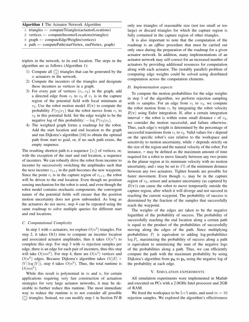
Algorithm 1 The Actuator Network Algorithm1: triangles ← computeTriangles(actuatorLocations)2: vertices ← computeIncenterLocations(triangles)3: graph ← computeEdgeWeights(vertices)4: path ← computePath(startVertex, endVertex, graph)

triplets in the network, to its end location. The steps in thealgorithm are as follows (Algorithm 1):

1) Compute all(n3

)triangles that can be generated by the

n actuators in the network.2) Compute the incenters of the triangles and designate

these incenters as vertices in a graph.3) For every pair of vertices (v1, v2) in the graph, add

a directed edge from v1 to v2 if v1 is in the captureregion of the potential field with local minimum atv2. Use the robot motion model R(v) to compute theprobability P (v2|v1) that the robot moves from v1 tov2 in this potential field. Set the edge weight to be thenegative log of this probability: − logP (v2|v1).

4) The weighted graph forms a roadmap for the robot.Add the start location and end location to the graphand run Dijkstra’s algorithm [16] to obtain the optimalpath from start to goal, or, if no such path exists, theempty sequence.

The resulting shortest path is a sequence {vi} of vertices, or,with the exception of the start and end location, a sequenceof incenters. We can robustly drive the robot from incenter toincenter by successively switching the amplitudes such thatthe next incenter vi+1 in the path becomes the new waypoint.Since the point vi is in the capture region of vi+1, the robotwill be driven to the end location. Even though no positionsensing mechanism for the robot is used, and even though therobot model contains stochastic components, the convergentnature of the potential fields will ensure that the positionmotion uncertainty does not grow unbounded. As long asthe actuators do not move, step 4 can be repeated using thesame roadmap to solve multiple queries for different startand end locations.

C. Computational Complexity

In step 1 with n actuators, we explore O(n3) triangles. Forstep 2, it takes O(1) time to compute an incenter locationand associated actuator amplitudes, thus it takes O(n3) tocomplete this step. For step 3 with m rejection samples peredge, there is an edge for each pair of incenters, thus this stepwill take O(mn6). For step 4, there are O(n3) vertices andO(n6) edges. Because Dijkstra’s algorithm takes O(|E| +|V | log |V |), step 4 takes O(n6). Thus, the total runtime isO(mn6).

While this result is polynomial in m and n, for certainapplications requiring very fast construction of actuationstrategies for very large actuator networks, it may be de-sirable to further reduce this runtime. The most immediateway to reduce the runtime is to not consider all possible(n3

)triangles. Instead, we can modify step 1 in Section IV-B

only use triangles of reasonable size (not too small or toolarge) or discard triangles for which the capture region isfully contained in the capture region of other triangles.

It is also important to note that the computation of theroadmap is an offline procedure that must be carried outonly once during the preparation of the roadmap for a givenactuator network. In addition, many implementations of anactuator network may self-correct for an increased number ofactuators by providing additional resources for computationalong with each actuator. The (notably parallel) problem ofcomputing edge weights could be solved using distributedcomputation across the computation elements.

D. Implementation aspects

To compute the motion probabilities for the edge weightsin step 3 of the algorithm, we perform rejection samplingwith m samples. For an edge from v1 to v2, we computethe robot motion from v1 by integrating the robot velocityR(v) using Euler integration. If, after a certain integrationinterval τ the robot is within some small distance ε of v2,we consider the motion successful, and failure otherwise.Thus, each edge’s weight is determined by the percentage ofsuccessful transitions from v1 to v2. Valid values for ε dependon the specific robot’s size relative to the workspace andsensitivity to motion uncertainty, while τ depends strictly onthe size of the region and the natural velocity of the robot. Forinstance, τ may be defined as the maximum amount of timerequired for a robot to move linearly between any two pointsin the planar region at its minimum velocity with no motionuncertainty, and ε may be set to 1% of the minimum distancebetween any two actuators. Tighter bounds are possible forfaster movement. Even though v1 may be in the captureregion of v2, sensor and actuator uncertainty (as captured byR(v)) can cause the robot to move temporarily outside thecapture region, after which it will diverge and not succeed inreaching the current waypoint. The probability of success isdetermined by the fraction of the samples that successfullyreach the waypoint.

The weights of the edges are taken to be the negativelogarithm of the probability of success. The probability ofsuccessfully reaching the end location along a certain pathis equal to the product of the probabilities of successfullymoving along the edges of the path. Since multiplyingprobabilities Pi is equivalent to adding log-probabilitieslogPi, maximizing the probability of success along a pathis equivalent to minimizing the sum of the negative logsof the probabilities along a path. Thus, we can efficientlycompute the path with the maximum probability by usingDijkstra’s algorithm from p0 to pe using the negative log ofthe probability at each edge.

V. SIMULATION EXPERIMENTS

All simulation experiments were implemented in Matlaband executed on PCs with a 2.0GHz Intel processor and 2GBof RAM.

We fixed the workspace to be 5×5 units, and used m = 10rejection samples. We explored the algorithm’s effectiveness

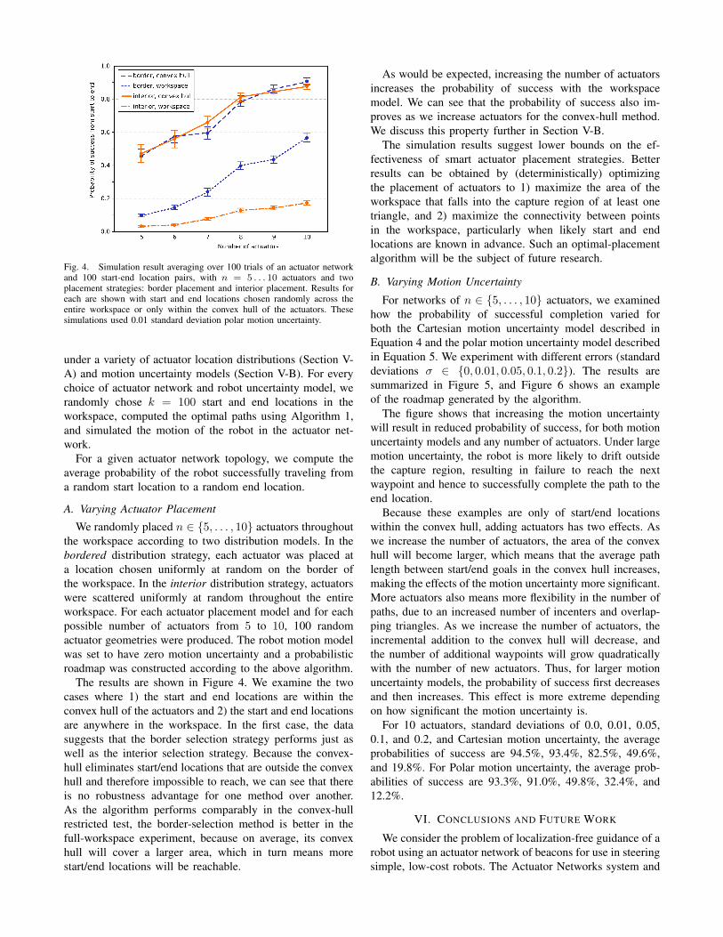
Fig. 4. Simulation result averaging over 100 trials of an actuator networkand 100 start-end location pairs, with n = 5 . . . 10 actuators and twoplacement strategies: border placement and interior placement. Results foreach are shown with start and end locations chosen randomly across theentire workspace or only within the convex hull of the actuators. Thesesimulations used 0.01 standard deviation polar motion uncertainty.

under a variety of actuator location distributions (Section V-A) and motion uncertainty models (Section V-B). For everychoice of actuator network and robot uncertainty model, werandomly chose k = 100 start and end locations in theworkspace, computed the optimal paths using Algorithm 1,and simulated the motion of the robot in the actuator net-work.

For a given actuator network topology, we compute theaverage probability of the robot successfully traveling froma random start location to a random end location.

A. Varying Actuator Placement

We randomly placed n ∈ {5, . . . , 10} actuators throughoutthe workspace according to two distribution models. In thebordered distribution strategy, each actuator was placed ata location chosen uniformly at random on the border ofthe workspace. In the interior distribution strategy, actuatorswere scattered uniformly at random throughout the entireworkspace. For each actuator placement model and for eachpossible number of actuators from 5 to 10, 100 randomactuator geometries were produced. The robot motion modelwas set to have zero motion uncertainty and a probabilisticroadmap was constructed according to the above algorithm.

The results are shown in Figure 4. We examine the twocases where 1) the start and end locations are within theconvex hull of the actuators and 2) the start and end locationsare anywhere in the workspace. In the first case, the datasuggests that the border selection strategy performs just aswell as the interior selection strategy. Because the convex-hull eliminates start/end locations that are outside the convexhull and therefore impossible to reach, we can see that thereis no robustness advantage for one method over another.As the algorithm performs comparably in the convex-hullrestricted test, the border-selection method is better in thefull-workspace experiment, because on average, its convexhull will cover a larger area, which in turn means morestart/end locations will be reachable.

As would be expected, increasing the number of actuatorsincreases the probability of success with the workspacemodel. We can see that the probability of success also im-proves as we increase actuators for the convex-hull method.We discuss this property further in Section V-B.

The simulation results suggest lower bounds on the ef-fectiveness of smart actuator placement strategies. Betterresults can be obtained by (deterministically) optimizingthe placement of actuators to 1) maximize the area of theworkspace that falls into the capture region of at least onetriangle, and 2) maximize the connectivity between pointsin the workspace, particularly when likely start and endlocations are known in advance. Such an optimal-placementalgorithm will be the subject of future research.

B. Varying Motion Uncertainty

For networks of n ∈ {5, . . . , 10} actuators, we examinedhow the probability of successful completion varied forboth the Cartesian motion uncertainty model described inEquation 4 and the polar motion uncertainty model describedin Equation 5. We experiment with different errors (standarddeviations σ ∈ {0, 0.01, 0.05, 0.1, 0.2}). The results aresummarized in Figure 5, and Figure 6 shows an exampleof the roadmap generated by the algorithm.

The figure shows that increasing the motion uncertaintywill result in reduced probability of success, for both motionuncertainty models and any number of actuators. Under largemotion uncertainty, the robot is more likely to drift outsidethe capture region, resulting in failure to reach the nextwaypoint and hence to successfully complete the path to theend location.

Because these examples are only of start/end locationswithin the convex hull, adding actuators has two effects. Aswe increase the number of actuators, the area of the convexhull will become larger, which means that the average pathlength between start/end goals in the convex hull increases,making the effects of the motion uncertainty more significant.More actuators also means more flexibility in the number ofpaths, due to an increased number of incenters and overlap-ping triangles. As we increase the number of actuators, theincremental addition to the convex hull will decrease, andthe number of additional waypoints will grow quadraticallywith the number of new actuators. Thus, for larger motionuncertainty models, the probability of success first decreasesand then increases. This effect is more extreme dependingon how significant the motion uncertainty is.

For 10 actuators, standard deviations of 0.0, 0.01, 0.05,0.1, and 0.2, and Cartesian motion uncertainty, the averageprobabilities of success are 94.5%, 93.4%, 82.5%, 49.6%,and 19.8%. For Polar motion uncertainty, the average prob-abilities of success are 93.3%, 91.0%, 49.8%, 32.4%, and12.2%.

VI. CONCLUSIONS AND FUTURE WORK

We consider the problem of localization-free guidance of arobot using an actuator network of beacons for use in steeringsimple, low-cost robots. The Actuator Networks system and

(a) Average success rate under Cartesian motion uncertainty.

(b) Average success rate under polar motion uncertainty.

Fig. 5. Comparison of the results of varying Gaussian motion uncertaintyfor a fixed set of actuator locations under two motion uncertainty models,with start and end locations chosen within the convex hull of the actuators.

algorithm steer unmonitored robots between points using anexternal network of actuators and a probabilistic roadmap.Our algorithm was able to produce relatively high proba-bilities of successful navigation between randomly-selectedpoints even in the presence of motion uncertainty.

The low number of actuators necessary for successfulsteering in our technique has important consequences for therobustness of these methods in practice. An inexpensive wayto guarantee continuous operation of an actuator network isto use more than the minimum number of actuators requiredfor high-probability performance; as an example, with 20actuators under border placement and 1% Cartesian motionuncertainty, even if half of the actuators eventually fail, theprobability of completion would not drop significantly.

We plan to explore several extensions in future work. Thetechnique of actuator networks can be extended to considerobstacles in the workspace. An obstacle can affect an Ac-tuator Network in three ways: (1) the obstacle restricts themotion of the mobile robot in the workspace, (2) the obstacleblocks the signal from an actuator, and (3) the obstacle causesmulti-path effects as the signals from the actuators reflectoff the obstacles. To model case 1, we can represent obsta-cles implicitly in the graph via the edge weights encoding

(a) Triangles and corresponding in-centers (denoted ∗) generated from8 randomly placed actuators.

(b) Roadmap showing edges be-tween incenters and an example path(thick line) through the network.

Fig. 6. Example of a simulation of the actuator-networks algorithm withn = 8 actuators and Cartesian motion uncertainty with σ = 0.01. Theactuators are placed randomly on the border of a square workspace, theincenters of all possible triangles between them form vertices in a roadmapwith edges containing the probability of successful transition by activationof an actuator triplet.

transition success probabilities. As discussed in Sec. IV-D,we estimate the probability P (v2|v1) of successfully movingfrom vertex v1 to vertex v2 by simulating the robot’s motionas it follows the gradient of the signal generated by theactuators. If the mobile robot’s motion intersects an obstacleduring a simulation, we determine that a failure has occurredin our rejection sampling step. For case 2, we can modifythe simulation so the gradient used by the mobile robot doesnot include signal from a particular actuator if a line segmentbetween that actuator and the mobile robot’s current locationintersects an obstacle. Since the probability of success foredges in the graph will decrease when obstacles are present,the number of actuators necessary in order to find a feasibleplan will increase. Case 3 is known to be difficult to modeleffectively, and is a significant problem for certain domainssuch as RSSI localization. As future work, we can alsoevaluate how different multi-path models will affect the robotby including this in the determination of the edge-weights ina similar fashion as case 2.

We would also like to explore the alternative problem ofdesigning an algorithm for placement of actuators.

VII. ACKNOWLEDGMENTS

We thank the members of the UC Berkeley AutomationSciences Lab for their feedback and support, includingparticularly helpful contributions from Ephrat Bitton, JijieXu, and Menasheh Fogel. We also thank Claire Tomlin, andShankar Sastry for their support.

REFERENCES

[1] O. D. Kellogg, “Foundations of potential theory,” 1969.[2] J. C. Maxwell, “On hills and dales,” The Philosophical Magazine,

vol. 40, no. 269, pp. 421–427, 1870.[3] H. Choset, K. M. Lynch, S. Hutchingson, G. Kantor, W. Burgand,

L. E. Kavraki, and S. Thrun, Principles of Robot Motion: Theory,Algorithms, and Implementations, 1st ed. MIT Press, 2005.

[4] O. Khatib, “Commande dynamique dans l’espace operationnel desrobots manipulateurs en presence d’obstacles,” Ph.D. dissertation,Ecole Nationale Superieure de l’Aeronautique et de l’Espace,Toulouse, France, 1980.

[5] ——, “Real-time obstacle avoidance for manipulators and mobilerobots,” The International Journal of Robotics Research, vol. 5, no. 1,pp. 90–98, 1986.

[6] C. Connolly, J. Burns, and R. Weiss, “Path planning using Laplace’sequation,” in Proceedings of the IEEE International Conference onRobotics and Automation, May 1990, pp. 2102–2106.

[7] W. S. Newman and N. Hogan, “High speed robot control and obstacleavoidance using dynamic potential functions,” in Proceedings of theIEEE International Conference on Robotics and Automation, 1987,pp. 14–24.

[8] E. Rimon and D. E. Koditschek, “Exact robot navigation usingartificial potential functions,” IEEE Trans. Robotics and Automation,vol. 8, no. 5, pp. 501–518, 1992.

[9] Q. Li, M. D. Rosa, and D. Rus, “Distributed algorithms for guidingnavigation across a sensor network,” in MobiCom ’03: Proceedingsof the 9th annual international conference on Mobile computing andnetworking. New York, NY, USA: ACM Press, 2003, pp. 313–325.

[10] L. C. A. Pimenta, G. A. S. Pereira, and R. C. Mesquita, “Fullycontinuous vector fields for mobile robot navigation on sequences ofdiscrete triangular regions,” in Proceedings of the IEEE InternationalConference on Robotics and Automation, 2007, pp. 1992–1997.

[11] K. F. Bohringer and H. Choset, Distributed Manipulation, 1st ed.Kluwer Academic Publishers, 2000.

[12] K.-F. Bhringer, V. Bhatt, B. R. Donald, and K. Goldberg, “Algorithmsfor sensorless manipulation using a vibrating surface,” Algorithmica,vol. 26, no. 3, pp. 389–429, April 2000.

[13] A. Sudsang and L. Kavraki, “A geometric approach to designing aprogrammable force field with a unique stable equilibrium for partsin the plane,” in Proceedings of the IEEE Interational Conference onRobotics and Automation, vol. 2, 2001, pp. 1079–1085.

[14] F. Lamiraux and L. E. Kavraki, “Positioning of symmetric andnon-symmetric parts using radial and constant fields: Computationof all equilibrium configurations,” International Journal of RoboticsResearch, vol. 20, no. 8, pp. 635–659, 2001.

[15] T. H. Vose, P. Umbanhowar, and K. M. Lynch, “Vibration-inducedfrictional force fields on a rigid plate,” in Proceedings of the IEEEInternational Conference on Robotics and Automation, April 2007,pp. 660–667.

[16] S. M. LaValle, Planning Algorithms. Cambridge, U.K.: CambridgeUniversity Press, 2006.

[17] B. Bouilly, T. Simeon, and R. Alami, “A numerical technique for plan-ning motion strategies of a mobile robot in presence of uncertainty,”in Proceedings of the IEEE International Conference on Robotics andAutomation, vol. 2, Nagoya, Japan, May 1995, pp. 1327–1332.

[18] S. M. LaValle and S. A. Hutchinson, “An objective-based frameworkfor motion planning under sensing and control uncertainties,” Inter-national Journal of Robotics Research, vol. 17, no. 1, pp. 19–42, Jan.1998.

[19] T. Dean, L. P. Kaelbling, J. Kirman, and A. Nicholson, “Planningunder time constraints in stochastic domains,” Artificial Intelligence,vol. 76, no. 1-2, pp. 35–74, Jul. 1995.

[20] D. Ferguson and A. Stentz, “Focussed dynamic programming: Exten-sive comparative results,” Robotics Institute, Carnegie Mellon Univer-sity, Pittsburgh, PA, Tech. Rep. CMU-RI-TR-04-13, Mar. 2004.

[21] R. Alterovitz, T. Simeon, and K. Goldberg, “The Stochastic MotionRoadmap: A sampling framework for planning with Markov motionuncertainty,” in Robotics: Science and Systems, 2007.

[22] A. Lazanas and J. Latombe, “Motion planning with uncertainty: Alandmark approach,” Artificial Intelligence, vol. 76, no. 1-2, pp. 285–317, 1995.