Active and passive damping systems for vibration control ......Active and passive damping systems...

Active and passive damping systems forvibration control of metal machiningequipment

Ole Christian Hermanrud

Master of Science in Mechanical Engineering

Supervisor: Bjørn Haugen, MTPCo-supervisor: Olav Egeland, IPK

Dan Östling, Sandvik Teeness AS

Department of Mechanical and Industrial Engineering

Submission date: May 2017

Norwegian University of Science and Technology

AcknowledgementsI would like to express my gratitude to my supervisor Bjørn Haugen for his supervisionand help during this thesis. His contributions have been much needed and greatly valued.He made sure that the paper would be my own work, but steered me in the right thedirection whenever he thought I needed it. He was also very understanding during thedifficult times while working with the thesis.

I would also like to thank Dan Østling for his input and ideas. He has played an importantrole in enabling me to finish the thesis. All the employees at Teeness have been veryhelpful and interested in finding the best solution.

Finally, I must express my very profound gratitude to my parents and to my spousefor providing me with unfailing support and continuous encouragement throughout myyears of study and through the process of researching and writing this thesis. Thisaccomplishment would not have been possible without them. Thank you.


i

Active and passive damping systems for vibrationcontrol of metal machining equipment


Abstract

Passive damping is used to reduce vibrations of machining tools. The drawback with thepassive damping system is that it is adjusted to damp out vibrations in one restrictedfrequency range. Active damping uses real time measurements to dampen the vibrationsand is not tuned for one specific frequency range. Teeness AS wants to be able to investi-gate different ways of regulating an active damping system on a physical test bench andto investigate if an Arduino is suited for regulating the system.

This paper presents the design development of the physical test bench, simulations of thedesigned test bench and an electrical setup with Arduino as the regulating controller.

Actuators were evaluated and purchased. The test bench was designed to fit the actuatorsusing Siemens NX as CAD program. The components of the test bench were producedby Teeness AS. Simulations of the designed test bench were conducted using FEDEM toinvestigate the dynamics of the system. Requirements for the Arduino were investigatedand regulating scripts were coded, tested and evaluated.

The simulated test bench was able to significantly reduce the vibrations investigated.However there were some behaviours of the simulated test bench that differ from themeasurements made of the physical test bench. This was most likely a result of themodeling of actuators. The results from the simulations give an indication of the generalbehaviour of the test bench, but the use of exact values should be avoided. To improvethe validity of the simulations, further work with the simulation of the actuators shouldbe conducted. Using an Arduino as a control mechanism seems promising, but furtherwork needs to be done to reduce the noise of the sensor data and the regulating scriptpresented in this paper should be improved.

ii

Active and passive damping systems for vibrationcontrol of metal machining equipment


Sammendrag

Passiv demping er brukt for a redusere vibrasjoner pa metal bearbeidende verktœy. Ulem-pen med passive dempesystem er at systemet er justert for a dempe ut vibrasjoner rundten gitt frekvens. Aktiv demping pa den andre siden bruker natids data for a regulereet system som demper ut vibrasjoner og er ikke avhengig av a bli justert for en bestemtfrekvens. Teeness AS ønsker a undersøke forskjellige mater a regulere et aktivt dem-pesystem pa en fysisk testbenk og a undersøke om det er mulig a bruke Arduino somreguleringsmekanisme.

Denne oppgaven presenterer utviklingen av den fysiske testbenken, simuleringer av denmodellerte testbenken og et elektrisk oppsett der en Arduino er brukt for a reguleresystemet.

Aktuatorer ble evaluert og anskaffet. Deretter ble testbenken designet rundt aktuatoreneved a bruke Siemens NX som modelleringsverktøy. Delene modellert ble produsert avTeeness AS. Simuleringer av den modellerte testbenken ble gjennomført i FEDEM for aundersøke de dynamiske egenskapene til testbenken. Krav til Arduino ble undersøkt ogskript ble laget og evaluert.

Den simulerte testbenken kunne redusere de undersøkte vibrasjonene signifikant. Det varnoe avvik fra simuleringer og resultater fra testing av den fysiske testbenken. Avviketoppstar mest sannsynlig grunnet modellering av aktuator ikke er slik som i virkeligheten.Eksakte verdier fra simuleringer blir da ikke vektlagts, men fokus er pa den generelleoppførselen. Videre arbeid med modellering av aktuatorer er anbefalt for fa mere repre-sentative simuleringer. A bruke Arduino som kontroll mekanisme viker lovende. Viderearbeid med a redusere støy og forbedring av script ma gjennomføres for a gi en sikkerkonklusjon pa om Arduino er egnet eller ikke.

iii

Contents

Acknowledgements i

Abstract ii

Sammendrag iii

List of Figures vi

List of Tables viii

Abbreviations ix

1 Introduction 1

2 Theory 32.1 Arduino boards . . . . . . . . . . . . . . . . . . . . . . . . . . . . . . . . 32.2 Hook’s law . . . . . . . . . . . . . . . . . . . . . . . . . . . . . . . . . . . 52.3 Harmonic motion . . . . . . . . . . . . . . . . . . . . . . . . . . . . . . . 62.4 Newtons second law . . . . . . . . . . . . . . . . . . . . . . . . . . . . . . 72.5 Dynamics modeling of system . . . . . . . . . . . . . . . . . . . . . . . . 8

2.5.1 Spring . . . . . . . . . . . . . . . . . . . . . . . . . . . . . . . . . 82.5.2 Damper . . . . . . . . . . . . . . . . . . . . . . . . . . . . . . . . 102.5.3 Forced harmonic vibrations . . . . . . . . . . . . . . . . . . . . . 122.5.4 Support motion . . . . . . . . . . . . . . . . . . . . . . . . . . . . 152.5.5 System with two degrees of freedom . . . . . . . . . . . . . . . . . 172.5.6 Rayleigh damping . . . . . . . . . . . . . . . . . . . . . . . . . . . 19

2.6 Piezoelectric actuators . . . . . . . . . . . . . . . . . . . . . . . . . . . . 19

3 Test bench and virtual model setup 243.1 Choosing the actuator . . . . . . . . . . . . . . . . . . . . . . . . . . . . 263.2 Electrical setup . . . . . . . . . . . . . . . . . . . . . . . . . . . . . . . . 283.3 Mechanical setup . . . . . . . . . . . . . . . . . . . . . . . . . . . . . . . 30

3.3.1 Main mass . . . . . . . . . . . . . . . . . . . . . . . . . . . . . . . 313.3.2 Counter mass . . . . . . . . . . . . . . . . . . . . . . . . . . . . . 323.3.3 Rubber sandwich . . . . . . . . . . . . . . . . . . . . . . . . . . . 333.3.4 Spring . . . . . . . . . . . . . . . . . . . . . . . . . . . . . . . . . 36

iv

Contents v

3.4 The simulation setup . . . . . . . . . . . . . . . . . . . . . . . . . . . . . 393.4.1 Rubber modeling . . . . . . . . . . . . . . . . . . . . . . . . . . . 413.4.2 The actuator . . . . . . . . . . . . . . . . . . . . . . . . . . . . . 45

4 Tests, calibrations and scripts 504.1 Noise in the circuit . . . . . . . . . . . . . . . . . . . . . . . . . . . . . . 51

4.1.1 Noise between accelerometer and Arduino . . . . . . . . . . . . . 514.1.2 Noise in the rest of the circuit . . . . . . . . . . . . . . . . . . . . 52

4.2 Time used by functions in script . . . . . . . . . . . . . . . . . . . . . . . 534.3 Accelerometer . . . . . . . . . . . . . . . . . . . . . . . . . . . . . . . . . 554.4 Scripts used in the Arduino Due . . . . . . . . . . . . . . . . . . . . . . . 62

4.4.1 Frequency and amplitude estimation . . . . . . . . . . . . . . . . 624.4.2 Stroke of actuator . . . . . . . . . . . . . . . . . . . . . . . . . . . 634.4.3 Regulating output signal . . . . . . . . . . . . . . . . . . . . . . . 644.4.4 Initiating the signal . . . . . . . . . . . . . . . . . . . . . . . . . . 67

4.5 Adjusting properties in the simulations . . . . . . . . . . . . . . . . . . . 69

5 Results 735.1 Active damping simulations . . . . . . . . . . . . . . . . . . . . . . . . . 73

5.1.1 Amplitude of stack displacement . . . . . . . . . . . . . . . . . . 745.1.2 Phase specter resulting in vibration reduction . . . . . . . . . . . 765.1.3 Change in frequency affects the delay specter . . . . . . . . . . . 775.1.4 Effect of change in amplitude . . . . . . . . . . . . . . . . . . . . 77

5.2 Active damping regulation . . . . . . . . . . . . . . . . . . . . . . . . . . 795.2.1 Measurement of frequencies . . . . . . . . . . . . . . . . . . . . . 795.2.2 Reading the frequency with Arduino . . . . . . . . . . . . . . . . 805.2.3 Calculating the acceleration with Arduino . . . . . . . . . . . . . 805.2.4 Applying regulating signal in correct phase . . . . . . . . . . . . 81

6 Discussion 846.1 Simulations . . . . . . . . . . . . . . . . . . . . . . . . . . . . . . . . . . 846.2 Test bench as demonstrator for active damping . . . . . . . . . . . . . . 876.3 Arduino as control mechanism . . . . . . . . . . . . . . . . . . . . . . . . 90

7 Conclusion and Further Work 93

A Appendix 95

Bibliography 99

List of Figures

2.1 Layout of the Arduino Due board. . . . . . . . . . . . . . . . . . . . . . . 32.2 PWM used to represent a quasi-sine wave form. . . . . . . . . . . . . . . 42.3 Acceleration-frequency relationship with 420µm amplitude . . . . . . . . 82.4 Different types of damping models[1] . . . . . . . . . . . . . . . . . . . . 92.5 Model of mass-spring system . . . . . . . . . . . . . . . . . . . . . . . . . 92.6 Model of mass-spring-damper system . . . . . . . . . . . . . . . . . . . . 102.7 Vector relationship between spring-, damping force and force caused by

acceleration . . . . . . . . . . . . . . . . . . . . . . . . . . . . . . . . . . 132.8 Phase shift between applied force and oscillation of mass . . . . . . . . . 142.9 Amplified force in a mass-spring-damper system with damping coefficients

from 0.01 to 0.1 . . . . . . . . . . . . . . . . . . . . . . . . . . . . . . . . 152.10 Model of a mass-spring-damper system with oscillating base . . . . . . . 152.11 Model of a two mass-spring system . . . . . . . . . . . . . . . . . . . . . 172.12 Typical hysteresis of Piezoelectric stack[2] . . . . . . . . . . . . . . . . . 212.13 Typical relationship between applied force and stroke of a piezoelectric

actuator[2] . . . . . . . . . . . . . . . . . . . . . . . . . . . . . . . . . . . 212.14 Working curve of piezoelectric stack with mass load[2] . . . . . . . . . . . 22

3.1 Simple model of the dynamic representation . . . . . . . . . . . . . . . . 253.2 Actuator without protective cover . . . . . . . . . . . . . . . . . . . . . . 263.3 Simplified layout of the electrical circuit . . . . . . . . . . . . . . . . . . 283.4 Simple model of the test bench . . . . . . . . . . . . . . . . . . . . . . . 303.5 Design of the main mass . . . . . . . . . . . . . . . . . . . . . . . . . . . 323.6 Design of the rubber sandwich . . . . . . . . . . . . . . . . . . . . . . . . 353.7 Illustration of distance the bolt can be screwed . . . . . . . . . . . . . . . 373.8 Physical test bench . . . . . . . . . . . . . . . . . . . . . . . . . . . . . . 383.9 Components in the FEDEM simulation . . . . . . . . . . . . . . . . . . . 393.10 Deformations from simulation in NX, fixed bottom and free displacement

in x-y plane on top . . . . . . . . . . . . . . . . . . . . . . . . . . . . . . 423.11 Deformations from simulation in NX, fixed bottom and fixed in x-y plane

on top . . . . . . . . . . . . . . . . . . . . . . . . . . . . . . . . . . . . . 423.12 Deformations in eigenmode analysis with RBE2 elements . . . . . . . . . 443.13 Deformations in eigenmode analysis with RBE3 elements . . . . . . . . . 443.14 Compression of rubber. . . . . . . . . . . . . . . . . . . . . . . . . . . . . 453.15 Render of the flexure . . . . . . . . . . . . . . . . . . . . . . . . . . . . . 46

vi

List of Figures vii

3.16 Comparing displacements of the sphere. Flexure modelled as one partcompared with eight parts . . . . . . . . . . . . . . . . . . . . . . . . . . 46

3.17 FEDEM model of the flexure in eight parts . . . . . . . . . . . . . . . . . 473.18 Displacement of sphere with force and displacement regulation using values

from data sheet. . . . . . . . . . . . . . . . . . . . . . . . . . . . . . . . . 48

4.1 Script for measuring the time consumption for code instructions . . . . . 534.2 Signal from ADXL335 at 1g acceleration at various frequencies . . . . . . 564.3 Signal from ADXL335 while mounted on shaker with 10Hz frequency and

varying acceleration . . . . . . . . . . . . . . . . . . . . . . . . . . . . . . 564.4 Signal from ADXL335 while mounted on shaker with 50Hz frequency and



varying acceleration . . . . . . . . . . . . . . . . . . . . . . . . . . . . . . 584.7 Relationship between acceleration and analog read value . . . . . . . . . 594.8 Relationship between analogRead()-value amplitude and frequency . . . . 604.9 Script calculating the frequency . . . . . . . . . . . . . . . . . . . . . . . 634.10 Voltage displacement relationship of actuators . . . . . . . . . . . . . . . 654.11 Script for the ωt-sine representation . . . . . . . . . . . . . . . . . . . . . 664.12 Script for the matrix-element sine representation . . . . . . . . . . . . . . 674.13 Script determining when to initiate the regulating signal . . . . . . . . . 684.14 Results from Vibration View, frequency sweep at 0.1g acceleration without

damping components . . . . . . . . . . . . . . . . . . . . . . . . . . . . . 694.15 Results from FEDEM, frequency sweep at 0.1g acceleration without damp-

ing components before adjustments . . . . . . . . . . . . . . . . . . . . . 704.16 Results from FEDEM, frequency sweep at 0.1g acceleration without damp-

ing components after adjustments . . . . . . . . . . . . . . . . . . . . . . 714.17 Results from Vibration View, frequency sweep at 0.1g acceleration with

damping components . . . . . . . . . . . . . . . . . . . . . . . . . . . . . 714.18 Results from FEDEM, frequency sweep at 0.1g acceleration with damping

components . . . . . . . . . . . . . . . . . . . . . . . . . . . . . . . . . . 72

5.1 Amplitude for main body with varying amplitudes regulating the piezo-electric stack-function . . . . . . . . . . . . . . . . . . . . . . . . . . . . . 75

5.2 Fraction of phase vs. amplification of vibrations . . . . . . . . . . . . . . 765.3 Displacement of main mass with and without damping by actuators . . . 775.4 Specter of phase delay with vibration reduction for different frequencies . 785.5 Maximum deviation from applied frequency fro oscilioscope and estimated

frequency by Arduino . . . . . . . . . . . . . . . . . . . . . . . . . . . . . 815.6 Error occurring as a result of time used by code instructions. . . . . . . . 825.7 Measured maximum error compared to calculated maximum error. . . . . 83

6.1 Maximum acceleration exerted by the shaker which the actuators candampen optimally . . . . . . . . . . . . . . . . . . . . . . . . . . . . . . . 89

List of Tables

2.1 Arduino boards with key properties . . . . . . . . . . . . . . . . . . . . . 5

3.1 Properties of PK2FVF1 actuator[3] . . . . . . . . . . . . . . . . . . . . . 273.2 Properties of PK2FVP1 stack[3] . . . . . . . . . . . . . . . . . . . . . . . 273.3 Values used for calculating thickness of counter mass . . . . . . . . . . . 333.4 Cross section area dimensions for rubber . . . . . . . . . . . . . . . . . . 343.5 Material properties for different rubbers . . . . . . . . . . . . . . . . . . 343.6 Material properties used for the parts used in the simulations . . . . . . . 393.7 Deviation in properties used in parts in simulation compared with data sheet 48

4.1 Data from noise test of the ADXL326 accelerometer . . . . . . . . . . . . 524.2 Data from noise test of the ADXL335 accelerometer . . . . . . . . . . . . 524.3 Time in µs used by code instructions . . . . . . . . . . . . . . . . . . . . 544.4 Tests conducted to investigate accelerometer data precision . . . . . . . . 554.5 The percentage change of analogRead()-value due to increasing acceleration 594.6 R2 values for the different accelerations . . . . . . . . . . . . . . . . . . . 614.7 Applied voltage and corresponding displacement of actuators . . . . . . . 644.8 analogWrite()value, arduino voltage, amplified voltage . . . . . . . . . . 644.9 Delay in matrix-element script and corresponding frequency. . . . . . . . 66

5.1 Input for sine function governing the base excitation function(SI units) . 745.2 Frequencies and corresponding minimum and maximum phase delay . . . 785.3 Reduction(negative values) and gain(positive values) of displacement am-

plitude . . . . . . . . . . . . . . . . . . . . . . . . . . . . . . . . . . . . . 795.4 Acceleration calculated with Arduino . . . . . . . . . . . . . . . . . . . . 81

viii

Abbreviations

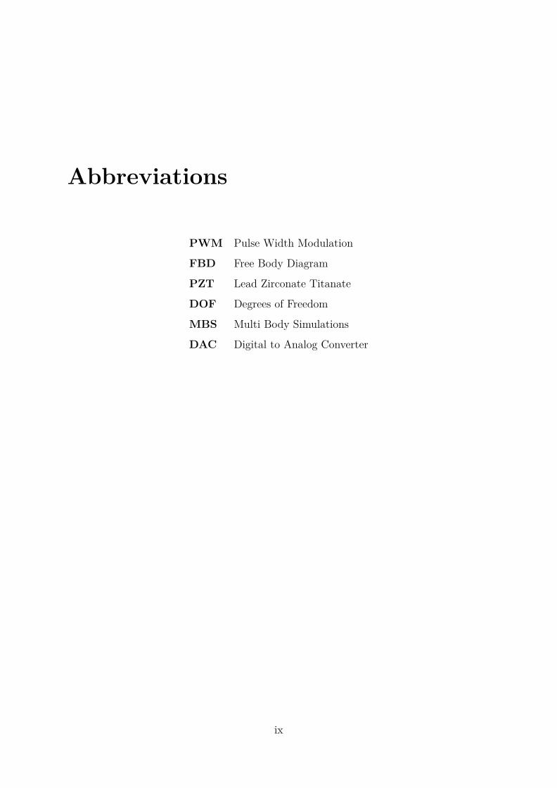
PWM Pulse Width Modulation

FBD Free Body Diagram

PZT Lead Zirconate Titanate

DOF Degrees of Freedom

MBS Multi Body Simulations

DAC Digital to Analog Converter

ix

Chapter 1

Introduction

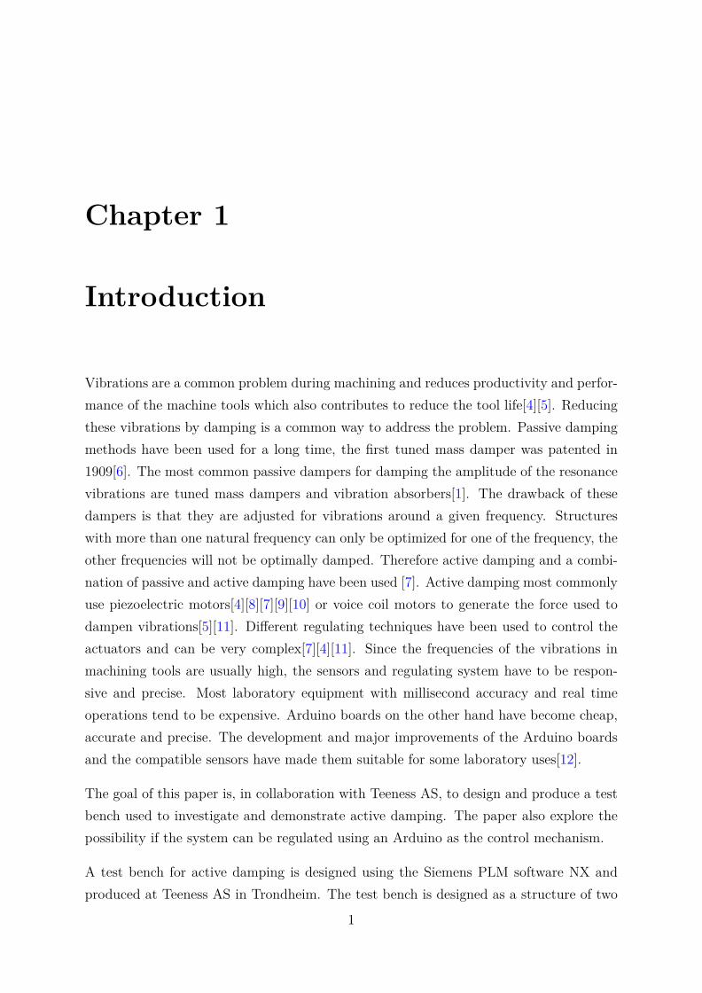
Vibrations are a common problem during machining and reduces productivity and perfor-mance of the machine tools which also contributes to reduce the tool life[4][5]. Reducingthese vibrations by damping is a common way to address the problem. Passive dampingmethods have been used for a long time, the first tuned mass damper was patented in1909[6]. The most common passive dampers for damping the amplitude of the resonancevibrations are tuned mass dampers and vibration absorbers[1]. The drawback of thesedampers is that they are adjusted for vibrations around a given frequency. Structureswith more than one natural frequency can only be optimized for one of the frequency, theother frequencies will not be optimally damped. Therefore active damping and a combi-nation of passive and active damping have been used [7]. Active damping most commonlyuse piezoelectric motors[4][8][7][9][10] or voice coil motors to generate the force used todampen vibrations[5][11]. Different regulating techniques have been used to control theactuators and can be very complex[7][4][11]. Since the frequencies of the vibrations inmachining tools are usually high, the sensors and regulating system have to be respon-sive and precise. Most laboratory equipment with millisecond accuracy and real timeoperations tend to be expensive. Arduino boards on the other hand have become cheap,accurate and precise. The development and major improvements of the Arduino boardsand the compatible sensors have made them suitable for some laboratory uses[12].

The goal of this paper is, in collaboration with Teeness AS, to design and produce a testbench used to investigate and demonstrate active damping. The paper also explore thepossibility if the system can be regulated using an Arduino as the control mechanism.

A test bench for active damping is designed using the Siemens PLM software NX andproduced at Teeness AS in Trondheim. The test bench is designed as a structure of two

1

Chapter 1 2

masses, one large and one small. The large mass is placed on a rubber cylinder fastenedto a shaker. The base excitation of the shaker causes vibrations to the large mass andactuators, fastened to the large mass, regulate the displacement of the small mass todampen the vibrations of the large mass.

Scripts on an Arduino Due board were used to investigate whether the regulation of theactive damping system could be performed with satisfying results. The data used in thescripts are read from Arduino compatible components.

Multi body simulations(MBS) are simulations that are composed of elastic bodies and arelation described between them. The test bench consists of many parts and MBS aretherefore used to investigate the properties. FEDEM was the chosen MBS program usedfor simulating the virtual the bench. Components were investigated and modified bythem selves and later joined together in simulations containing all parts.

Chapter 2

Theory

2.1 Arduino boards

Arduino boards are cheap multipurpose micro controller boards that are designed to beuser friendly[13]. On the boards there are pins to connect to components as sensors oractuators. The digital pins are I/O pins, meaning that they have two states, on and off.While the I/O pin is on, a current is sent through the pin usually, 5V or 3.3V, dependingon the board and its configurations. The I/O pins can also measure voltages wherethe signal is read as either ”High”(1) when there is a measurable current or ”Low”(0)otherwise.

Figure 2.1: Layout of the Arduino Due board.

3

Chapter 2 4

The analog input pins can measure the current and return a value between 0 and thehighest number the resolution of the analog to digital converter(ADC) allows. This valueis function of the bit resolution of the board and is given by equation 2.1.

Resolution = 2bits (2.1)

Some pins have the possibility of using pulse width modulation(PMW) and can give anaverage output between 0V and maximum output voltage of the board. The resolutionfor these regulations are also determined by equation 2.1.

PWM is a technique using digital means to represent analogue values. The current isswitched on and off at a high frequency and the relationship between the on/off timedetermines the average current. With this control mechanism a quasi-sine wave form canbe generated[14]. An analog signal would give the desired voltage as a continuous signaland not a signal that alters between 0V and the maximum voltage the board can deliver.

Figure 2.2: PWM used to represent a quasi-sine wave form.

There are over 20 different original Arduino boards and countless clones. Table 2.1 showssome of the Arduino broads available and some of their key properties[15]. The CPU speeddetermines how many instructions per second the Arduino is capable of executing. Theflash memory (program space), is where the Arduino sketch is stored, while the SRAM(static random access memory) is where the sketch creates and manipulates variableswhen it runs[16]. A sketch is the name that Arduino uses for a program. It is the codethat is uploaded to and run on an Arduino board[17]. ”Analog in/out” in the table showshow many digital to analog converter pins the board has. For the Arduino Due these pinsprovide true analog outputs with 12-bits resolution (4096 levels) with the analogWrite()function and not a value represented by using PWM. The DAC output range is actuallyfrom 0.55V to 2.75V on the Due.

Chapter 2 5

Table 2.1: Arduino boards with key properties

Name CPU Analog in/out Bit resolution SRAM[kB] Flash[kB]Uno 16 MHz 6/0 8 2 32Due 84 MHz 12/2 12 96 512

Mega 16 MHz 16/0 8 8 256Mini 16 MHz 8/0 8 2 32

Arduino uses a scripting language that is based on C/C++ and open source librarieswith scripts are available on-line[18].There is a large open source community, where trou-bleshooting and examples of scripts are posted. Some instructions in the codes in theArduino language such as ”micros()”, which returns the number of microseconds sincethe Arduino started running, has a resolution dependent on the CPU speed.

There are many Arduino compatible components and modules available, making proto-typing convenient as there is a large variety of components to choose from. There areanalog devices which are passive, and there are modules that have small processors thatprocess data before sending the data to the Arduino board. Signals from components aresent digitally, analogue or via serial communication.

2.2 Hook’s law

Using springs, the relationship between applied force and the displacement of a homo-geneous material was discovered to be dependent on the stiffness of the material [19].Hook’s law states that the force by a solid (in compression or tension) is proportional tothe product of the body’s stiffness and its displacement. This can be generally expressedby equation 2.2[20].

Force = Stiffness ∗Displacement (2.2)

Hook’s law is valid for linear elastic materials. The unload curve of these materials followthe load curve, while no plasticity has occurred. Equation 2.2 is valid for both compressionand tension as long as the material has linear elastic behaviour. The direction of the forceby the body is in the opposite direction of applied displacement relative to its equilibrium.

Hooke’s law can be written asσ = Eε (2.3)

Chapter 2 6

Where σ is the stress, E is the Young’s modulus and ε is strain. The relationship betweenthe axial force, F, on a solid and the stress is shown below[21].

F = σA (2.4)

Where A is the cross section area of the body. Strain is defined as the length of thedeformation relative to the original length.

ε = δ

L (2.5)

Combining equations 2.3, 2.4 and 2.5 yields equation 2.6[22].

F = δEAL (2.6)

Equation 2.6 shows the relation between compression- of tension force needed to deforma body with a constant cross section area. This means that the material stiffness can beexpressed by

k = EAL (2.7)

The pressure needed to compress a solid body with the displacement δ will then beexpressed with

p = F

A= AEδ

AL= Eδ

L(2.8)

The relationship between the modulus of elasticity and the share modulus in isotropicmaterials is given by equation 2.9.[23]

G = E

2(1 + ν) (2.9)

2.3 Harmonic motion

When the motion of an object is repeated regularly in equal intervals of time τ , its motionis considered as periodic. The time for one repetition of the motion is called the period,denoted here by τ . Its reciprocal is called the frequency, f.

Chapter 2 7

f = 1τ

(2.10)

Harmonic motion is the simplest form of periodic motion [24] and can be expressed by

x = Asin(2π tτ

) (2.11)

The angular velocity is denoted with ω and measured in radians per second.

ω = 2πf (2.12)

By combining equation 2.12 and 2.10 we get the equation for harmonic motion

x = Asin(ωt) (2.13)

with its derivatives which describe the velocity and the acceleration of the harmonicmotion.

x = ωAcos(ωt) (2.14)

x = -ω2Asin(ωt) = -ω2x (2.15)

From this we can see that the acceleration is heavily affected by the angular velocity andthereby the frequency of the harmonic motion. The relationship between acceleration andfrequency is represented in figure 2.3. Angular velocity is used to describe the frequencyusing radians pr second.

2.4 Newtons second law

The force needed to accelerate an object is proportional to the product of the objectsmass and the acceleration. Thus;

F = ma (2.16)

Where F represents force, m represents mass, and a represents the acceleration.

Chapter 2 8

Figure 2.3: Acceleration-frequency relationship with 420µm amplitude

2.5 Dynamics modeling of system

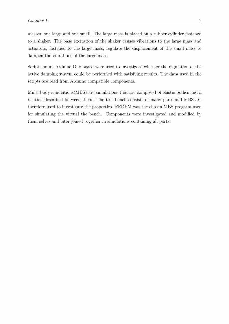
There are many different ways to regulate vibrations of a mass[1]. The motion of thebody in a mass-spring-damper system is dependent on its mass, spring stiffness, dampingcoefficients and applied forces. Figure 2.4 shows different ways to regulate the oscillationsin the main mass by damping. In the representation shown in the figure, it is assumedthat the ground has a harmonic single degree of freedom(DOF) motion and there are noexternal forces. The figure shows graphs of the amplification of a relative motion of thelarge mass, M, compared to the motion of the ground(y-axis) and the frequency of theoscillation of the support structure(x-axis). The peaks of the relative displacement occuron the natural frequency/frequencies of the systems.

2.5.1 Spring

Springs follow Hook’s law and the force-displacement relation by a spring is given byequation 2.17

F = kx (2.17)

Where F represents force, k represents the spring stiffness, and x represents the displacement[25].

When looking at a mas spring system with no damper or external forces acting on thesystem, we can obtain the equations of motion from the free body diagram(FBD). The

Chapter 2 9

Figure 2.4: Different types of damping models[1]

Figure 2.5: Model of mass-spring system

equation of motions is obtained by balancing the forces acting on the body. When themass is stationary, the gravitational force, mg is equal to the reaction force by the springgiven by equation 2.17, thus;

k∆ = mg (2.18)

When the displacement of the mass relative to its stationary position is denoted by x, andusing Newton’s second law of motion 2.16 we obtain the equation of motion by lookingat the FBD.

mx = mg − k(∆ + x) (2.19)

Chapter 2 10

Subsituting equation 2.18 into eqation 2.19 we obtain

mx = −kx (2.20)

By including equation 2.15 we get

−mω2x = −kx (2.21)

solving for ω

ω =√k

m(2.22)

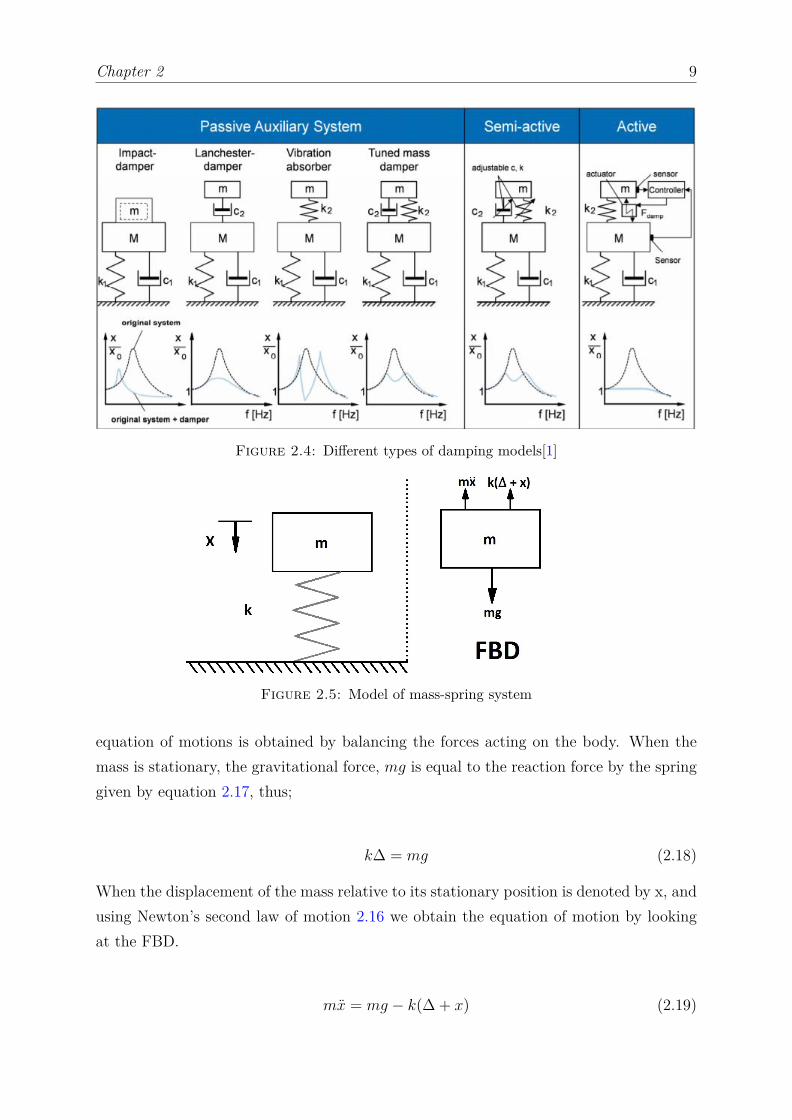
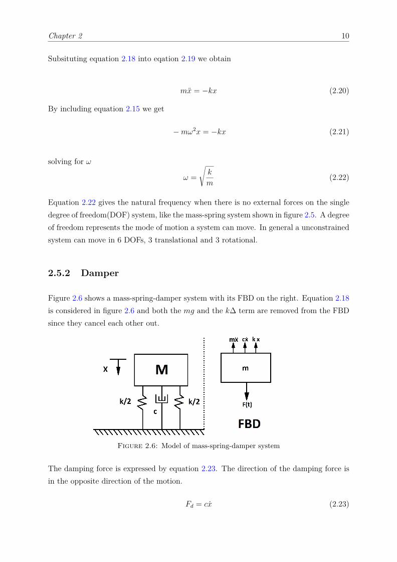
Equation 2.22 gives the natural frequency when there is no external forces on the singledegree of freedom(DOF) system, like the mass-spring system shown in figure 2.5. A degreeof freedom represents the mode of motion a system can move. In general a unconstrainedsystem can move in 6 DOFs, 3 translational and 3 rotational.

2.5.2 Damper

Figure 2.6 shows a mass-spring-damper system with its FBD on the right. Equation 2.18is considered in figure 2.6 and both the mg and the k∆ term are removed from the FBDsince they cancel each other out.

Figure 2.6: Model of mass-spring-damper system

The damping force is expressed by equation 2.23. The direction of the damping force isin the opposite direction of the motion.

Fd = cx (2.23)

Chapter 2 11

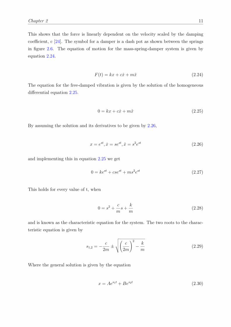
This shows that the force is linearly dependent on the velocity scaled by the dampingcoefficient, c [24]. The symbol for a damper is a dash pot as shown between the springsin figure 2.6. The equation of motion for the mass-spring-damper system is given byequation 2.24.

F (t) = kx+ cx+mx (2.24)

The equation for the free-damped vibration is given by the solution of the homogeneousdifferential equation 2.25.

0 = kx+ cx+mx (2.25)

By assuming the solution and its derivatives to be given by 2.26,

x = est, x = sest, x = s2est (2.26)

and implementing this in equation 2.25 we get

0 = kest + csest +ms2est (2.27)

This holds for every value of t, when

0 = s2 + c

ms+ k

m(2.28)

and is known as the characteristic equation for the system. The two roots to the charac-teristic equation is given by

s1,2 = − c

2m ±

√√√√( c

2m

)2

− k

m(2.29)

Where the general solution is given by the equation

x = Aes1t +Bes2t (2.30)

Chapter 2 12

By combining the expressions for s1 and s2 from equation 2.29 to 2.30 we can rewrite2.30.

x = e− c2m

t(Ae√

(( c2m

)2− km

)t +Be−√

(( c2m

)2− km

)t) (2.31)

By investigating equation 2.31 we can see that when the term ( c2m)2 − k

m is positive,the exponents in the large parenthesis in equation 2.31 are real numbers and thereforeequation 2.31 can only yield positive values. The first term in equation 2.31 e− c

2m t is adecreasing function when t increases. When the ( c

2m)2− km term is positive, the magnitude

of the decreasing exponent in the function is reduced and the system is referred to as aover damped system[26].

If the exponent in equation 2.31 is complex, the equation has both positive and negativevalues, meaning oscillation will occur. This case is referred to as under damped.

If ( c2m)2 − k

m is 0, the motion is described by e− c2m t and the amplitudes A and B. This

case is called critical damped and occurs when

(c

2m

)2

= k

m(2.32)

The damping coefficient yielding critical damping is therefor given by

cc = 2mωn = 2√km (2.33)

Damping can then be expressed in relation to the critical damping and called dampingratio and is denoted with ξ. Materials have an internal damping that is often denoted byusing a %-based value.

ξ = c

cc(2.34)

2.5.3 Forced harmonic vibrations

As seen from previous subsection the FBD in figure 2.6 show us that the equation ofmotion can be expressed by by equation 2.35 [25]. During forced harmonic vibrationsfunction describing the external forces F (t) is not equal to 0.

Chapter 2 13

F (t) = kx+ cx+mx (2.35)

The function describing the forced harmonic vibrations is expressed with an amplitude ofF0 and an angular velocity is given by ωt, the differential equation describing the motionof the FBD will be 2.36

F0sin(ωt) = kx+ cx+mx (2.36)

We can assume the particular solution to be of the form[24].

x = Xsin(ωt− φ) (2.37)

Where X is the amplitude, φ is the phase and x expresses the displacement. The velocityis given by 2.38 and the acceleration is given by 2.39.

x = ωXcos(ωt− φ) (2.38)

x = −ω2Xsin(ωt− φ) (2.39)

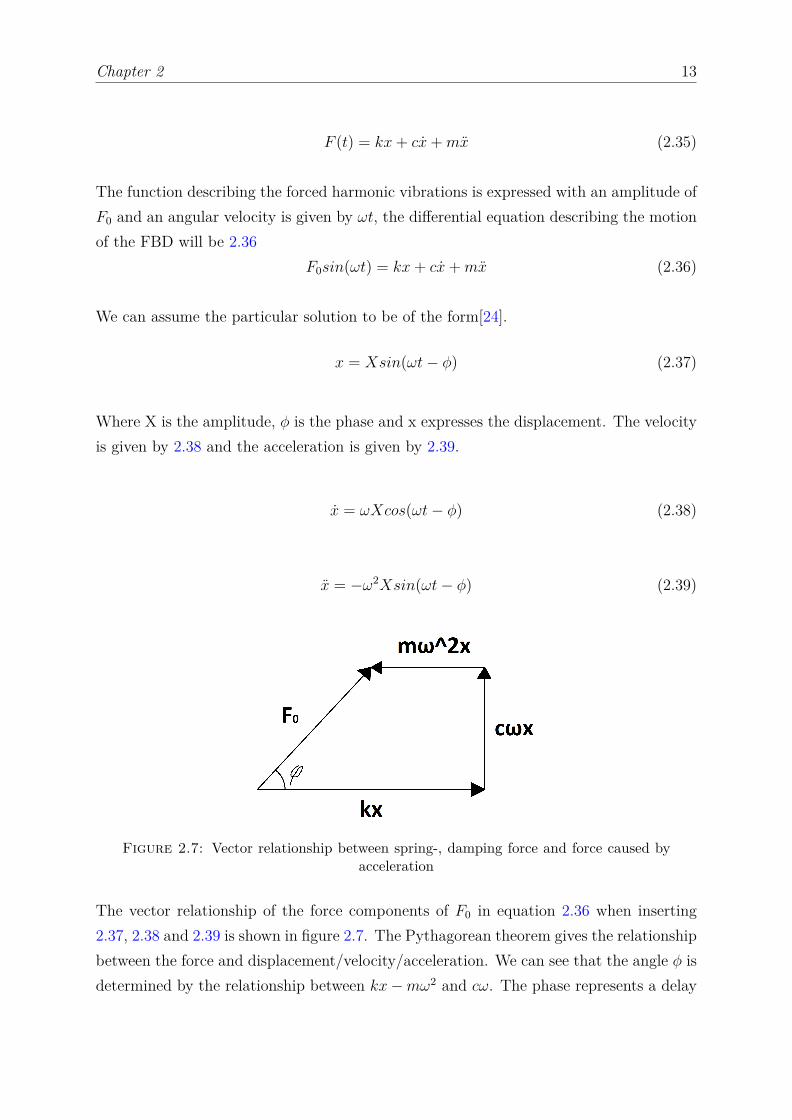
Figure 2.7: Vector relationship between spring-, damping force and force caused byacceleration

The vector relationship of the force components of F0 in equation 2.36 when inserting2.37, 2.38 and 2.39 is shown in figure 2.7. The Pythagorean theorem gives the relationshipbetween the force and displacement/velocity/acceleration. We can see that the angle φ isdetermined by the relationship between kx−mω2 and cω. The phase represents a delay

Chapter 2 14

in the oscillation of the mass applied force. Figure 2.8 shows a the motion of the massand the applied force with a 45 degree phase shift, which is when cω is equal to kx−mω2.

Figure 2.8: Phase shift between applied force and oscillation of mass

F 20 = (X((k −mω2))2 + (cω)2) (2.40)

F 20 = X2(k −mω2)2 +X2(cω)2 (2.41)

F0 = X√

(k −mω2)2 + (cω)2 (2.42)

X = F0√(k −mω2)2 + (cω)2

(2.43)

Deviding the numerator and denominator by k, we obtain:

X =F0k√

(1− mω2

k)2 + ( cω

k)2

(2.44)

When including equations 2.34, 2.33 and 2.22 and moving the F0k term over to the left

side of the equation to make the equation non-dimensional we get

Chapter 2 15

kX

F0= 1√

(1− ( ωωn

)2)2 + (2ξ ωωn

)2(2.45)

This equation describes the amplification of the force in the spring in proportion to theharmonic exited force on the mass. In other words this shows the amplified force on themass due to the systems natural frequencies.

Equation 2.45 is shown in the figure 2.9 below with different damping ratios.

Figure 2.9: Amplified force in a mass-spring-damper system with damping coefficientsfrom 0.01 to 0.1

2.5.4 Support motion

Figure 2.10: Model of a mass-spring-damper system with oscillating base

When the ground in which the mass is supported by is moving, the mass also will move.The motion of the mass relative to the ground will be given by equation 2.46.

Chapter 2 16

z = x− y (2.46)

The case where the motion of the ground is harmonic and is given by equation

y = Y sin(ωt) (2.47)

y = ωY cos(ωt) (2.48)

y = −ω2Y sin(ωt) (2.49)

Using the FBD of the model, we can obtain the equation of motion.

mx = −k(x− y)− c(x− y) (2.50)

Combining equations 2.50, 2.46 and 2.49 we can rewrite the equation to 2.51

mz + cz + kz = mω2Y sin(ωt) (2.51)

Equation 2.51 is similar to equation 2.36. The differences are that the variable x describingthe motion of the body is substituted with z describing the relative distance between thebody and the oscillating base. F0 is substituted for mω2Y. Making the same assumptionas discussed in section 2.5.3, the amplitude is given by equation 2.52.

Z = mω2Y√(k −mω2)2 + (cω)2

(2.52)

The steady state amplitude can be derived by using exponential form to describe themotion and substituting into equation 2.50. This leads to the amplitude given by equation2.53.

∣∣∣∣XY∣∣∣∣ =

√√√√ k2 + (ωc)2

(k −mω2)2 + (cω)2 (2.53)

Chapter 2 17

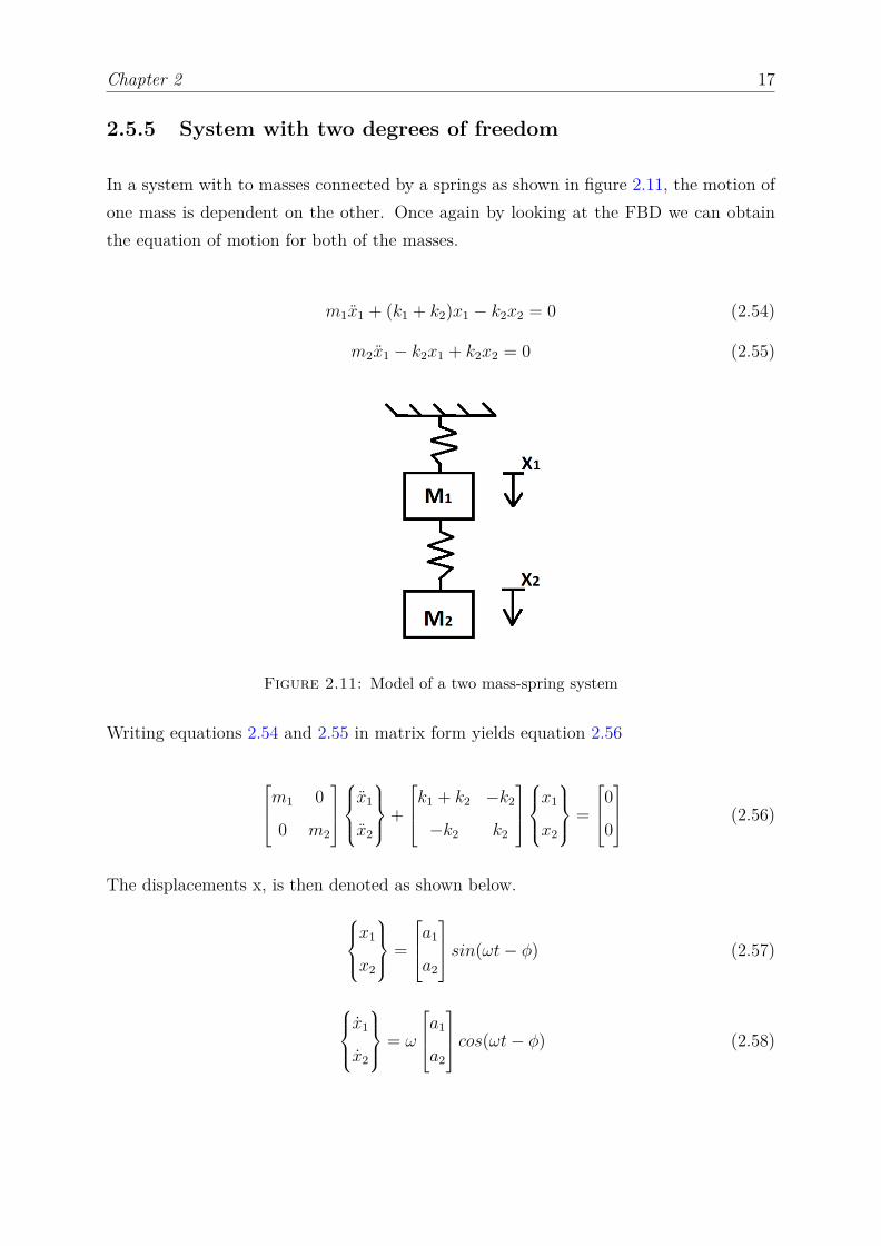
2.5.5 System with two degrees of freedom

In a system with to masses connected by a springs as shown in figure 2.11, the motion ofone mass is dependent on the other. Once again by looking at the FBD we can obtainthe equation of motion for both of the masses.

m1x1 + (k1 + k2)x1 − k2x2 = 0 (2.54)

m2x1 − k2x1 + k2x2 = 0 (2.55)

Figure 2.11: Model of a two mass-spring system

Writing equations 2.54 and 2.55 in matrix form yields equation 2.56

m1 0

0 m2

x1

x2

+

k1 + k2 −k2

−k2 k2

x1

x2

=

0

0

(2.56)

The displacements x, is then denoted as shown below.x1

x2

=

a1

a2

sin(ωt− φ) (2.57)

x1

x2

= ω

a1

a2

cos(ωt− φ) (2.58)

Chapter 2 18

x1

x2

= −ω2

a1

a2

sin(ωt− φ) (2.59)

Combining the equations above gives

− ω2

m1 0

0 m2

a1

a2

sin(ωt− φ) +

k1 + k2 −k2

−k2 k2

a1

a2

sin(ωt− φ) =

0

0

(2.60)

Deviding by sin(ωt - φ) gives

− ω2

m1 0

0 m2

a1

a2

+

k1 + k2 −k2

−k2 k2

a1

a2

=

0

0

(2.61)

Collecting the terms will give−ω2m1 + k1 + k2 −k2

−k2 −ω2m2 + k2

a1

a2

=

0

0

(2.62)

Solving for a1 and a2

det

∣∣∣∣∣∣∣−ω2m1 + k1 + k2 −k2

−k2 −ω2m2 + k2

∣∣∣∣∣∣∣ = 0 (2.63)

Giving the characteristic equation 2.64

(-ω2m1+k1+k2)(-ω2m2 + k2)-(-k2)(-k2) = 0 (2.64)

simplifying this equation gives

-ω4(m1m2)+-ω2(m2k1 + m2k2+ m1k2)+ k1k2= 0 (2.65)

To find the natural frequency we have to find the roots of equation 2.65. When the twonatural frequencies are found, we can values in equation 2.62. We can then calculate theamplitude ratio by dividing the amplitudes with each other.

Chapter 2 19

2.5.6 Rayleigh damping

Rayleigh damping, or proportional damping, consists of two proportional relations, mass-and stiffness proportional damping. Rayleigh damping is given by equation 2.66.

C = α1m+ α2k (2.66)

Where α1 and α2 are constants given by equations 2.67 and 2.68, m is the mass and k thestiffness. λi are the damping ratios for the selected vibration modes which are expressedwith the internal damping given in equation 2.34. This is used in FEDEM where neededtheory is provided in the FEDEM theory guide.

α1 = 2ω1ω2

ω22 − ω2

1(λ1ω2 − λ2ω1) (2.67)

α2 = 2(λ1ω2 − λ2ω1)ω2

2 − ω21

(2.68)

2.6 Piezoelectric actuators

Piezoelectrics either produce a voltage in response to mechanical stress, direct mode, ora physical displacement as a result of an applied electrical field, indirect mode. Due tothis property, piezoelectric materials are used in both actuators and sensors. One of themost common piezoelectric materials is lead-zirconate-titanate (PZT).

The piezoelectric effect, which can be described through a coupling the electric fieldequations with the strain tensor of HookeâĂŹs law that is shown below[8][9].

Dε

=

eσ dd

dc sE

Eσ

(2.69)

Here D is the electric displacement vector, ε is the strain vector, E is the applied electricfield vector, σm is the stress vector, eσij is the dielectric permittivity, ddim and dcjk are thepiezoelectric coefficients, and sEkm is the elastic compliance.

Chapter 2 20

There are 3 main categories for PZT actuators: low voltage, high voltage, and ringactuators. For any given height, h, of an actuator, a stacked device can produce adisplacement proportional to the number of stacks, as described by equation 2.70:

∆h = nd33V (2.70)

Here n is the number of stacks and the change in height is proportional to the number ofstacks. These stacked structures require a low driving voltage and have a quick responsetime whilst having a high force generation. The driving voltage for one stack and theresponse time is the same as the whole stack structure because the stacks are coupled inparallel.

Low voltage actuators tend to have operating voltages below 200 V. These devices aremonolithic stacks devices, meaning that the stacked structure is produced through sin-tering rather than gluing individual layers. They have an electrical capacitance on theorder of a few ÂţF and tend to have a high elastic modulus.

PZTs are often used where precision is key and are also capable of producing high forceswhile the stiffness is high. Piezoelectric actuator have been used by NASA to stabilizeinstruments during take of.

The hysteresis loop of a open-loop system will be similar to the one shown in figure2.12[2]. The three different curves show the hysteresis loop with different maximumvoltages applied. The hysteresis will be affected by the load applied and environmentalconditions.

The force the actuator can generate and the stroke is dependent on the load applied. Thegraph below shows a typical relationship between the stroke and the force applied on theactuator.

When no forces are applied on the actuator, the maximum stroke is achieved when apply-ing the maximum operating voltage. This stroke length is referred to as the free stroke∆LFS. The block force, FBlock is defined as the force needed to be applied to compressthe the actuator back to its original length after the maximum operational voltage isapplied. The stiffness of the actuator can be calculated by using the free stroke and theblocking force[2].

kA = FBlock∆LFS

(2.71)

Chapter 2 21

Figure 2.12: Typical hysteresis of Piezoelectric stack[2]

Figure 2.13: Typical relationship between applied force and stroke of a piezoelectricactuator[2]

The stroke and the force of the actuator is dependent on the load applied. If the loadapplied on the actuator behaves like a spring, the length of the stroke will be given byequation 2.71 and the force will be given by equation 2.73

Chapter 2 22

∆L ≈ ∆LFS(

kAkA + kL

)(2.72)

∆Feff = FBlock

(kL

kA + kL

)(2.73)

We see that the stroke is reduced when the stiffness of the load spring increases. This isbecause of the force the spring exerts back on the piezo.

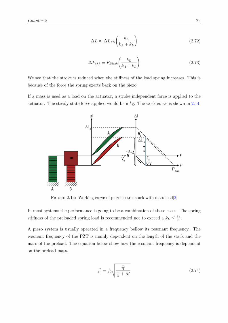
If a mass is used as a load on the actuator, a stroke independent force is applied to theactuator. The steady state force applied would be m*g. The work curve is shown in 2.14.

Figure 2.14: Working curve of piezoelectric stack with mass load[2]

In most systems the performance is going to be a combination of these cases. The springstiffness of the preloaded spring load is recommended not to exceed a kL ≤ kA

10 .

A piezo system is usually operated in a frequency bellow its resonant frequency. Theresonant frequency of the PZT is mainly dependent on the length of the stack and themass of the preload. The equation below show how the resonant frequency is dependenton the preload mass.

f′

0 = f0

√√√√ m3

m3 +M

(2.74)

Chapter 2 23

Where M is the preloaded mass, m is the mass of the actuator and f0 is the resonantfrequency with no load. For primarily dynamic applications, the lowest resonant fre-quency of the piezo with preload must be well above the driving frequency of the piezoactuator[27]. The time it takes the piezo to expand is given by

t ≈ 13f0

(2.75)

The maximum velocity of the actuator is dependent on the peak current of the powersupply used to regulate the actuator. The acceleration response is dependent on the slewrate of the power supply.

The necessary current to drive the actuator in a sine motion is given by the formula 2.76

IMax = πfCVpp (2.76)

The maximum power needed for the same operation is given by

PMax = πfCV 2pp (2.77)

Where C is the capacitance, Vpp is the peak-to-peak voltage and f is the frequency.

PZTs are brittle and have a low tensile strength. The stacks are not designed to withstandlateral, transverse of bending forces. Therefore most of the actuator have a mountingsystem for external loads that ensures that only compression is possible.

The driving power source has to be able to output the required voltage at the requiredslew rate and with the desired current. The slew rate is given by

Slew rate = δV

δt= IMax

C(2.78)

The maximum bandwidth of the amplifier is then given by

fMax = IMax

πVPPC(2.79)

Chapter 3

Test bench and virtual model setup

Firstly an actuator that is suitable to regulate the counter mass with desired speed andprecision was chosen. The actuator had to be able to be regulated by simple means sothat an Arduino board could be used as the control unit.

Secondly sensors and equipment that were used to drive the motors were chosen. Theequipment to drive the actuator must satisfy the demands of the actuators.

After the components were chosen, the test bench was designed using Siemens NX. Thedesign was made considering the chosen components and how to mount them. Machinedrawings of the designed parts were made for production.

The virtual parts in NX were given material properties, meshed and used for MBS toinvestigate the dynamic and damping properties of the test bench.

The dynamic properties of the test bench as a whole were the main dimensioning criteria.Some off the criteria for the design are listed below.

1. The test bench was desired to have a natural frequency of around 100Hz-200Hz.

2. The mass of the test bench was desired to be fairly small and set to under 4kg.

3. Actuators have to be able to regulate the vibrations of the measured body.

4. The test bench has to be easily mounted on the shaker at Teeness’ laboratory.

The general design of the test bench is a two mass system where each mass has one DOF inthe same direction. The main mass was connected to a shaker by a rubber cylinder acting

24

Chapter 3 25

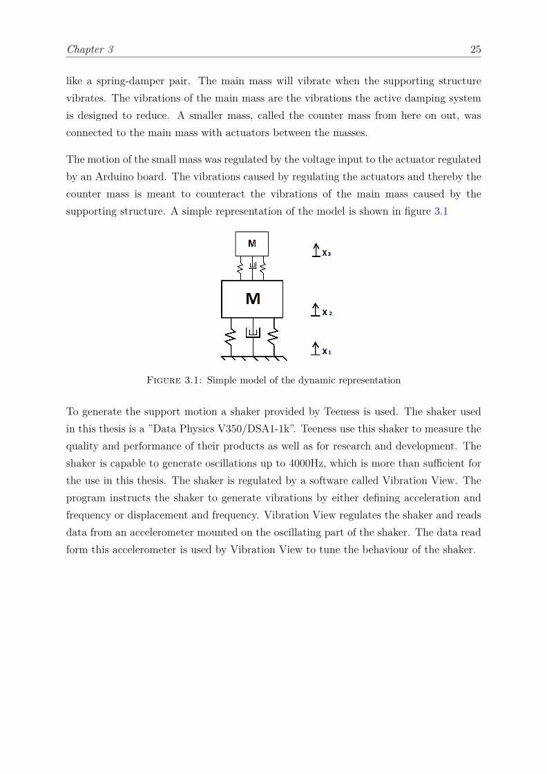
like a spring-damper pair. The main mass will vibrate when the supporting structurevibrates. The vibrations of the main mass are the vibrations the active damping systemis designed to reduce. A smaller mass, called the counter mass from here on out, wasconnected to the main mass with actuators between the masses.

The motion of the small mass was regulated by the voltage input to the actuator regulatedby an Arduino board. The vibrations caused by regulating the actuators and thereby thecounter mass is meant to counteract the vibrations of the main mass caused by thesupporting structure. A simple representation of the model is shown in figure 3.1

Figure 3.1: Simple model of the dynamic representation

To generate the support motion a shaker provided by Teeness is used. The shaker usedin this thesis is a ”Data Physics V350/DSA1-1k”. Teeness use this shaker to measure thequality and performance of their products as well as for research and development. Theshaker is capable to generate oscillations up to 4000Hz, which is more than sufficient forthe use in this thesis. The shaker is regulated by a software called Vibration View. Theprogram instructs the shaker to generate vibrations by either defining acceleration andfrequency or displacement and frequency. Vibration View regulates the shaker and readsdata from an accelerometer mounted on the oscillating part of the shaker. The data readform this accelerometer is used by Vibration View to tune the behaviour of the shaker.

Chapter 3 26

3.1 Choosing the actuator

The test bench was modelled to fit the actuators regulating the counter mass. Thereforeit was preferable that the actuator had a simple design with options for mounting. Thedesired frequencies in question are about 100Hz-200Hz, therefore the actuator had to beable to operate under these frequencies, preferably with a safety margin. The actuatorwas preferred to be fairly small, so that the actuator is easy to handle and that thedesigned test bench could be small. Reliability was also an important factor for ensuringan efficient regulating system. Furthermore the actuator had to provide a sufficient forceto dampen the oscillations of the main body when it was subjected to the vibrationscaused by the shaker. The actuator had to be able to be regulated by an Arduino andtherefor have a simple regulating mechanism or a simple driver that could use the signalsfrom the Arduino. The price was also important because the test bench was a prototypethat had no guarantee for being successful.

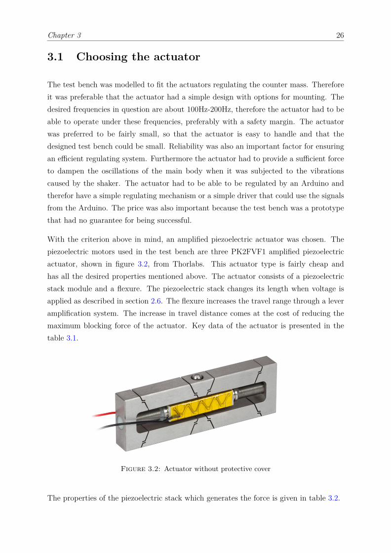
With the criterion above in mind, an amplified piezoelectric actuator was chosen. Thepiezoelectric motors used in the test bench are three PK2FVF1 amplified piezoelectricactuator, shown in figure 3.2, from Thorlabs. This actuator type is fairly cheap andhas all the desired properties mentioned above. The actuator consists of a piezoelectricstack module and a flexure. The piezoelectric stack changes its length when voltage isapplied as described in section 2.6. The flexure increases the travel range through a leveramplification system. The increase in travel distance comes at the cost of reducing themaximum blocking force of the actuator. Key data of the actuator is presented in thetable 3.1.

Figure 3.2: Actuator without protective cover

The properties of the piezoelectric stack which generates the force is given in table 3.2.

Chapter 3 27

Table 3.1: Properties of PK2FVF1 actuator[3]

Property ValueDrive voltage range Maximum: 0-75 V

Displacement (Free Stroke) av 75V 420µm + 15%Maximum push force in motion direction 100NMaximum pull force in motion direction 5N

Table 3.2: Properties of PK2FVP1 stack[3]

Property ValueDrive voltage range Maximum: 0-75 V

Displacement (Free Stroke) av 75V 44.8µm + 15%Maximum push force in motion direction 1000N

Capacitance 16.5 µF

As seen in the table 3.2, the driving voltage range is from 0V to 75V. Arduino boardscan only deliver up to 5V. Therefore, an amplifier to amplify the signal from the Arduinobecame a necessity. To drive these actuators the amplifier had to be able to deliversufficient current and be able to alter between these voltage levels as fast or faster thanthe Arduino. By rearranging equation 2.79, using the data in the data sheet for theactuator and assuming we want to be able to regulate the actuators up to 200Hz we cancalculate the required current.

IMax = fMax π VPP C = 200Hz π 75V 16.5µF = 0.78A (3.1)

The power needed to drive the actuator is given by equation 2.77

PMax = π 200 16.5µF (75V )2 = 58.3VA (3.2)

Chapter 3 28

3.2 Electrical setup

The sensors have to be fast, since the oscillations investigated are at a frequency upto 200Hz. The desired number of measurements for each oscillation is 20. The sensorsmust therefore be able to output values every 250µs with a satisfying resolution. Bothprecision and accuracy are desired, where precision is the most important. The scriptused to interpret data can adjust for the errors in the potential accuracy when sufficientlycalibrated. The sensors also had to be Arduino compatible so that sensors and theArduino can communicate. The sensors had to be small so that they could be mountedon the test bench without significantly changing the dynamic properties or design space.

Figure 3.3: Simplified layout of the electrical circuit

Two different accelerometers were chosen as sensors for the test bench, the ADXL335 andthe ADXL326. Both accelerometers are analog accelerometers meaning that they sendout a voltage continually while powered. The voltage varies between 0 and the voltageused to power the sensor(1.8V-3.6V). The ADXL335 can measure accelerations from -3gto 3g, while the ADXL326 can measure accelerations from -16g to 16g.

The chosen Arduino used for controlling the active damping system was the Arduino Due.The cost of this board is 36 euro compared to the 20 euro the original Arduino(UNO).The Properties that sets the Due apart from the other board is that it has analog outputsand a faster CPU than the other boards. This means that the calculations and actionsof the Arduino board is faster compared to the other boards. Further the resolution ofthe ”micros()”- function is 1µs compared to the resolution of UNO which returns values

Chapter 3 29

of multiples of 4µs. By having analog outputs the signal sent from the Arduino will be acontinuous voltage output and not a PWM as shown in figure 2.2. Since the output fromthe Arduino has to be amplified to drive the actuators, a continuous signal seems like amore reliable choice of regulation.

The amplifier used in the circuit is a ”Piezomechanic LE 200/150-1”. The data sheet forthe amplifier could not be found on the web page[28], so there is some uncertainty toits performance. The output voltage from the amplifier was measured with a multimeterbefore applied to the actuators. The slew rate/bandwidth is unknown for this amplifier.The demands for the amplifier are given 3.1 and 3.2.

The ADXL335 accelerometer was mounted on the main mass and was connected to theArduino with the jumper wires that came with the official Arduino beginners kit. TheADXL326 accelerometer was used to read the acceleration of the counter mass and there-for mounted on the counter mass. The Arduino processes the signals from the ADXL335accelerometer and sends out a signal that regulates the actuator via the DAC0 pin on theboard. Since the DAC pins on the Arduino only can output voltages between 0.55V and2.75V the signal has to be amplified. The amplifier is adjusted by manually adjusting thegain of the signal and the offset level. The output of the amplifier is directly coupled tothe three actuators using a modified coax cable.

Chapter 3 30

3.3 Mechanical setup

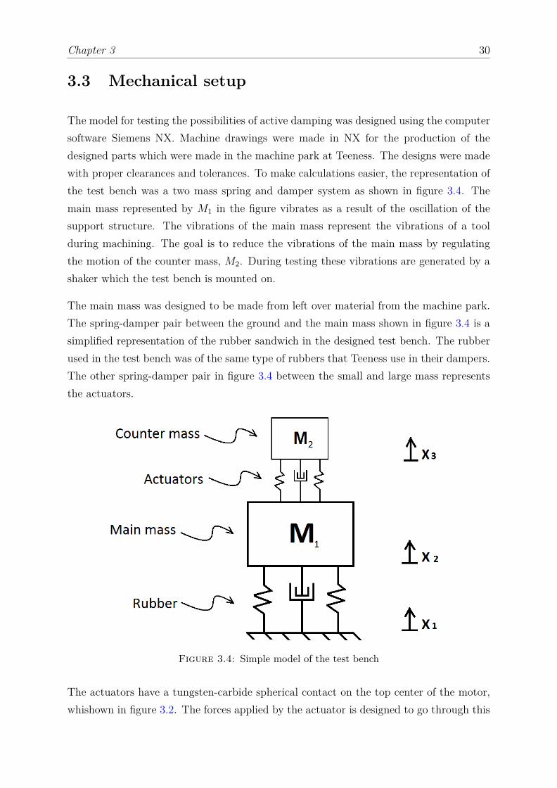
The model for testing the possibilities of active damping was designed using the computersoftware Siemens NX. Machine drawings were made in NX for the production of thedesigned parts which were made in the machine park at Teeness. The designs were madewith proper clearances and tolerances. To make calculations easier, the representation ofthe test bench was a two mass spring and damper system as shown in figure 3.4. Themain mass represented by M1 in the figure vibrates as a result of the oscillation of thesupport structure. The vibrations of the main mass represent the vibrations of a toolduring machining. The goal is to reduce the vibrations of the main mass by regulatingthe motion of the counter mass, M2. During testing these vibrations are generated by ashaker which the test bench is mounted on.

The main mass was designed to be made from left over material from the machine park.The spring-damper pair between the ground and the main mass shown in figure 3.4 is asimplified representation of the rubber sandwich in the designed test bench. The rubberused in the test bench was of the same type of rubbers that Teeness use in their dampers.The other spring-damper pair in figure 3.4 between the small and large mass representsthe actuators.

Figure 3.4: Simple model of the test bench

The actuators have a tungsten-carbide spherical contact on the top center of the motor,whishown in figure 3.2. The forces applied by the actuator is designed to go through this

Chapter 3 31

sphere. Since the force from each motor goes through the contact point connecting thesphere and the counter mass, balancing of the counter mass could be challenging withone motor. With one motor the counter mass would be free in all 3 rotational DOFsand extra boundary conditions would have to be made to keep the counter mass fromsliding off. Three motors were chosen to make sure that the motion of the counter massis translational and kept from sliding of, assuming all three motors behave identically.

Two accelerometers were mounted on the test bench. One on the counter mass and one onthe main mass. The accelerometer on the main mass sends data which is used to regulatethe actuators. The accelerometer on the top mass is there to enable the surveillance theacceleration of the counter mass.

3.3.1 Main mass

The main mass was made from left over material found at the workshop at Teeness. Thiswas done to keep the costs low. Since Teeness AS specialise in damping tools used inmetal working machines, including turning machines, they have bolts of both steel andaluminum which they use for production and testing. Their largest scrap bolts availablewere 100mm in diameter and this diameter was used to restrict the design space. Thebolt used for the main mass was turned from a initial diameter of 100mm to 95mm,this was done to ensure the bolt was circular. With a cross section that is circular theCNC-machining is independent of the rotation of the cross section of the bolt and lesstime for calibrating the CNC-machine is needed.

Three slots were milled for the actuators. The design enables the actuator to slide inthe slots, making it possible to regulate the distance from the center of the main massand the sphere of the actuator. Each actuator have two threaded M2.5 holes on thebottom of the protective cover which were used for mounting the actuator to the mainmass. Countersunk holes were drilled in the main mass in order to fasten the cover of theactuators to the main mass. The actuators can be mounted in three different places in theslot with different radii from the center of the main mass to the sphere of the actuator.The depth of the slots was made shallower than the height of the actuator. This was doneso that the sphere on the actuator in its fully retracted position is higher than the mainbody. This was done to ensure that the counter mass does not collide with the main masswhen in use. In the center of the main mass a M8 threaded hole was designed. This wasdone to be able to fasten a bolt that tightens a spring holding the counter mass in place.Three countersunk holes were made in the main mass for M5 screws to be able to fasten

Chapter 3 32

to the rubber sandwich to the main mass. Two threaded holes were mad on the side ofthe main mass to mount the ADXL335 accelerometer.

Figure 3.5: Design of the main mass

3.3.2 Counter mass

The counter mass should be approximately 115 of the main mass, which would be about

0.1kg. By looking at equation 2.74 we can see that a low mass is needed to keep resonantfrequency of the actuator high. As mentioned in section 2.6 the resonant frequency ofthe actuator is must be well above the driving frequency. The resonant frequency of theactuators with the counter mass is calculated below, with the assumption that the massis evenly distributed between the three actuators. The resonant frequency of the actuatoris over three times the maximal driving frequency and therefore considered to meet therequirements mentioned in section2.6.

f′

0 = 1000

√√√√ 0.073

0.073 + 0.033 = 642Hz (3.3)

The counter mass was made from excess material. The dimensions of the bolts availablewere the same as the bolts described for the main mass. The outer dimension wasmachined down to a diameter of 95mm. A hole with a diameter of 8.5mm in the center ofthe counter mass was made so that the M8 bolt tightening the spring holding the counter

Chapter 3 33

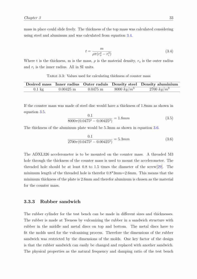
mass in place could slide freely. The thickness of the top mass was calculated consideringusing steel and aluminum and was calculated from equation 3.4.

t = m

ρπ(r2o − r2

i )(3.4)

Where t is the thickness, m is the mass, ρ is the material density, ro is the outer radiusand ri is the inner radius. All in SI units.

Table 3.3: Values used for calculating thickness of counter mass

Desired mass Inner radius Outer raduis Density steel Density aluminium0.1 kg 0.00425 m 0.0475 m 8000 kg/m3 2700 kg/m3

If the counter mass was made of steel disc would have a thickness of 1.8mm as shown inequation 3.5.

0.18000π(0.04752 − 0.004252) = 1.8mm (3.5)

The thickness of the aluminum plate would be 5.3mm as shown in equation 3.6.

0.12700π(0.04752 − 0.004252) = 5.3mm (3.6)

The ADXL326 accelerometer is to be mounted on the counter mass. A threaded M3hole through the thickness of the counter mass is used to mount the accelerometer. Thethreaded hole should be at least 0.8 to 1.5 times the diameter of the screw[29]. Theminimum length of the threaded hole is therefor 0.8*3mm=2.6mm. This means that theminimum thickness of the plate is 2.6mm and therefor aluminum is chosen as the materialfor the counter mass.

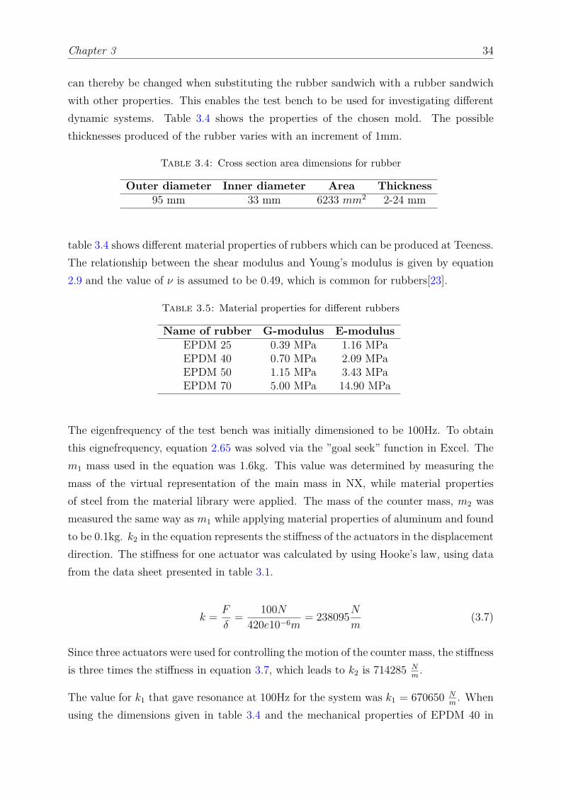
3.3.3 Rubber sandwich

The rubber cylinder for the test bench can be made in different sizes and thicknesses.The rubber is made at Teeness by vulcanizing the rubber in a sandwich structure withrubber in the middle and metal discs on top and bottom. The metal discs have tofit the molds used for the vulcanising process. Therefore the dimensions of the rubbersandwich was restricted by the dimensions of the molds. One key factor of the designis that the rubber sandwich can easily be changed and replaced with another sandwich.The physical properties as the natural frequency and damping ratio of the test bench

Chapter 3 34

can thereby be changed when substituting the rubber sandwich with a rubber sandwichwith other properties. This enables the test bench to be used for investigating differentdynamic systems. Table 3.4 shows the properties of the chosen mold. The possiblethicknesses produced of the rubber varies with an increment of 1mm.

Table 3.4: Cross section area dimensions for rubber

Outer diameter Inner diameter Area Thickness95 mm 33 mm 6233 mm2 2-24 mm

table 3.4 shows different material properties of rubbers which can be produced at Teeness.The relationship between the shear modulus and Young’s modulus is given by equation2.9 and the value of ν is assumed to be 0.49, which is common for rubbers[23].

Table 3.5: Material properties for different rubbers

Name of rubber G-modulus E-modulusEPDM 25 0.39 MPa 1.16 MPaEPDM 40 0.70 MPa 2.09 MPaEPDM 50 1.15 MPa 3.43 MPaEPDM 70 5.00 MPa 14.90 MPa

The eigenfrequency of the test bench was initially dimensioned to be 100Hz. To obtainthis eignefrequency, equation 2.65 was solved via the ”goal seek” function in Excel. Them1 mass used in the equation was 1.6kg. This value was determined by measuring themass of the virtual representation of the main mass in NX, while material propertiesof steel from the material library were applied. The mass of the counter mass, m2 wasmeasured the same way as m1 while applying material properties of aluminum and foundto be 0.1kg. k2 in the equation represents the stiffness of the actuators in the displacementdirection. The stiffness for one actuator was calculated by using Hooke’s law, using datafrom the data sheet presented in table 3.1.

k = F

δ= 100N

420e10−6m= 238095N

m(3.7)

Since three actuators were used for controlling the motion of the counter mass, the stiffnessis three times the stiffness in equation 3.7, which leads to k2 is 714285 N

m.

The value for k1 that gave resonance at 100Hz for the system was k1 = 670650 Nm

. Whenusing the dimensions given in table 3.4 and the mechanical properties of EPDM 40 in

Chapter 3 35

table 3.5 in a rearranged form of equation 2.7, be obtain the desirable length of the rubberprofile to be 19.4mm.

L = AE

k=

0.006233m22090000 Nm2

670650Nm

= 0.0194m = 19.4mm (3.8)

The rubbers produced at Teeness have a minimum thickness of 2mm with a thicknessincrement of 1mm. Therefor rounding 19.4 to the closest whole number, we get 19 whichwill be the length of the rubber in mm. This will lead to a slightly higher stiffness in therubber compared to its calculated length of 19.4mm. This will result in a slightly highernatural frequency, which can bee seen from equation 2.65.

Figure 3.6: Design of the rubber sandwich

While assuming that the shaker, which is the supporting structure of the test bench,oscillates at the test bench’s natural frequency with a constant acceleration, the acceler-ation of the main mass will be amplified. With the assumption of that the damping ofthe rubber is between 3-5% we can use equation 2.45 to see that the amplification ratiois between 10.0 and 16.7.

The disc on the top of the rubber has three threaded holes in which bolts going throughthe main mass is fastened with M5 bolts. The plate itself is only 5mm thick and thereforethe length of threaded area is equal to the diameter of the screw, which is almost theminimum thickness recommended for the threaded length for screw connections [29].The bottom disc of the rubber sandwich also has threaded holes so that it can be joinedto the first coupling disk with M5 screws. The coupling between the shaker and therubber sandwich is made out of two discs with a diameter of 120mm. These discs wereconnected to each other with M8 screws. The top plate has a M5 threaded hole to mountthe reference accelerometer used by Vibration View to tune the shaker.

Chapter 3 36

A key property of the rubber sandwich is that is is easily changed. If it is desired tochange the stiffness or the damping ratio of the rubber one can simply change the rubbersandwich.

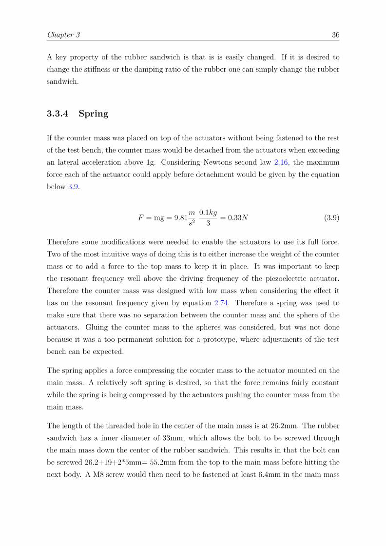
3.3.4 Spring

If the counter mass was placed on top of the actuators without being fastened to the restof the test bench, the counter mass would be detached from the actuators when exceedingan lateral acceleration above 1g. Considering Newtons second law 2.16, the maximumforce each of the actuator could apply before detachment would be given by the equationbelow 3.9.

F = mg = 9.81ms2

0.1kg3 = 0.33N (3.9)

Therefore some modifications were needed to enable the actuators to use its full force.Two of the most intuitive ways of doing this is to either increase the weight of the countermass or to add a force to the top mass to keep it in place. It was important to keepthe resonant frequency well above the driving frequency of the piezoelectric actuator.Therefore the counter mass was designed with low mass when considering the effect ithas on the resonant frequency given by equation 2.74. Therefore a spring was used tomake sure that there was no separation between the counter mass and the sphere of theactuators. Gluing the counter mass to the spheres was considered, but was not donebecause it was a too permanent solution for a prototype, where adjustments of the testbench can be expected.

The spring applies a force compressing the counter mass to the actuator mounted on themain mass. A relatively soft spring is desired, so that the force remains fairly constantwhile the spring is being compressed by the actuators pushing the counter mass from themain mass.

The length of the threaded hole in the center of the main mass is at 26.2mm. The rubbersandwich has a inner diameter of 33mm, which allows the bolt to be screwed throughthe main mass down the center of the rubber sandwich. This results in that the bolt canbe screwed 26.2+19+2*5mm= 55.2mm from the top to the main mass before hitting thenext body. A M8 screw would then need to be fastened at least 6.4mm in the main mass

Chapter 3 37

to satisfy the 0.8 times diameter criteria[29].This leads to that the remaining 48.8mm canbe used to adjust the compression of the spring as shown in figure 3.7.

Figure 3.7: Illustration of distance the bolt can be screwed

The total blocking force of the three actuators combined is at 300N. A spring with stiffness6700N

mwas used in the test bench to hold the counter mass in place. This would mean

that the screw had to compress the spring 22.4mm to pretension the spring with half ofthe blocking force(150N). This is shown in equation 2.17.

x = Fk

= 150N6700N

m

= 0.0224m (3.10)

The ISO standard for the pitch of the threads of an M8 are 1.25mm. This leads to thatthe bolt tightening the spring has to be turned 18 times to compress the spring with22.4mm. This would also result in the force form the spring by tightening the bolt withone revolution would be 8.4N.

The reduction of the stroke is given by equation 2.72. Inserting values from 3.7 gives thenew stroke length to be

L = 420µm 238095238095 + 6700 = 409µm (3.11)

This means that the difference in force by the spring when fully retracted compared tofully expanded is 2.73.

Chapter 3 38

∆F = 409µm6700Nm

= 2.73N (3.12)

The produced test bench mounted on the shaker is shown in figure 3.8.

Figure 3.8: Physical test bench

Chapter 3 39

3.4 The simulation setup

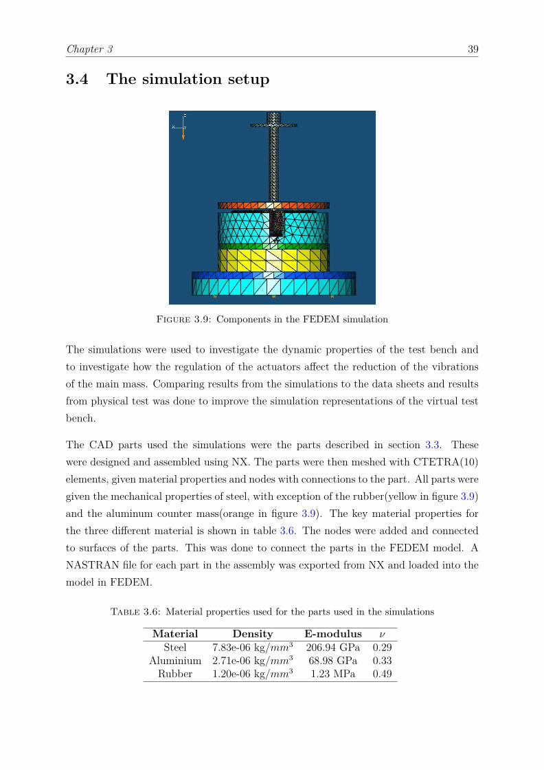
Figure 3.9: Components in the FEDEM simulation

The simulations were used to investigate the dynamic properties of the test bench andto investigate how the regulation of the actuators affect the reduction of the vibrationsof the main mass. Comparing results from the simulations to the data sheets and resultsfrom physical test was done to improve the simulation representations of the virtual testbench.

The CAD parts used the simulations were the parts described in section 3.3. Thesewere designed and assembled using NX. The parts were then meshed with CTETRA(10)elements, given material properties and nodes with connections to the part. All parts weregiven the mechanical properties of steel, with exception of the rubber(yellow in figure 3.9)and the aluminum counter mass(orange in figure 3.9). The key material properties forthe three different material is shown in table 3.6. The nodes were added and connectedto surfaces of the parts. This was done to connect the parts in the FEDEM model. ANASTRAN file for each part in the assembly was exported from NX and loaded into themodel in FEDEM.

Table 3.6: Material properties used for the parts used in the simulations

Material Density E-modulus νSteel 7.83e-06 kg/mm3 206.94 GPa 0.29

Aluminium 2.71e-06 kg/mm3 68.98 GPa 0.33Rubber 1.20e-06 kg/mm3 1.23 MPa 0.49

Chapter 3 40

FEDEM(Finite Element Dynamics in Elastic Mechanisms) is a MBS program designedfor solving dynamic problems. Imported parts are treated as individual objects and therelationship between these object are determined by interactions between triads set bythe user. Triads are connected to a node on a part and some connections between triadsdemand that the triads have the exact same coordinates. The interaction between thetriads can be determined by either joints, gears, springs or dampers.

A virtual spring was placed between the top of the bolt(grey in figure 3.9) and was giventhe stiffness of 6700 N

m. In the physical test bench the spring is compressed by screwing

the bolt with the spring between the washer and the counter mass. This was modeledin FEDEM by setting of initial stress free length to be longer than the initial length ofthe spring in the model. This would be the same as defining the original length of thespring to be the stress free length while the length of the spring in the model representsthe length of the compressed spring. The added stress free length to preload the springwas calculated to be 0.0224m in equation 3.10.

The steel parts in the model were connected by RBE2 connections in a rigid joint inFEDEM. Rigid joints are joints between two triads at the same coordinate. The jointhave all the relative translational- and rotational DOFs between the triads fixed, hence arigid connection between the two triads.

To represent the motion of the shaker, free joints were modeled to be at the bottommost plate in the numerical model. Free joints are joints between two triads where all6 DOFs are initially free, but can be altered by the user. This choice allows the user toset the relationship between triads to be free, fixed, prescribed or by a spring-damperrelationship. The motion of the shaker is modeled as a free joint where the only DOFthat is not fixed is in the z-direction(orange arrow) shown in figure 3.9. This motion isdetermined by a mathematical formula describing the oscillation of the virtual shaker.

Virtual sensors were added to triads to generate graphs of displacements, and to acquireacceleration data of the simulation. A control editor in FEDEM has to be used whenrequesting output from the sensors. The editor has different components that can beused to create a control system. These components can be used to model properties ofthe regulation system, such as delays and restrictions given by time response.

Rayleigh damping is used to simulate the internal proportional damping. Both stiffnessproportional and mass proportional damping was calculated for all parts using equations2.67 and 2.68.

Chapter 3 41

3.4.1 Rubber modeling

The rubber between the main mass and the shaker has a great influence on the dynamicsof the system. The stiffness of the rubber affects the eigenfrequency of the test bench andis represented as k2 in equation 2.65. The damping of the rubber determines how muchthe amplification of the force the main mass has compared to the base. How the rubberdeforms is also essential for the models used in the FEDEM simulations to represent thereal test bench. Firstly simulations were conducted to investigate the stiffness added bythe transverse constraints of the rubber body. Secondly the deformation mode of therubber was investigated in FEDEM. RBE2 and RBE3 connections used to couple thecenter node of the rubber to the surface area gave different deformation modes. Thirdlythe Young’s modulus of the material in the FEDEM model was adjusted to represent thestiffness of the transverse constrained rubber body with the selected RBE connection.

Stiffness of the rubber sandwich

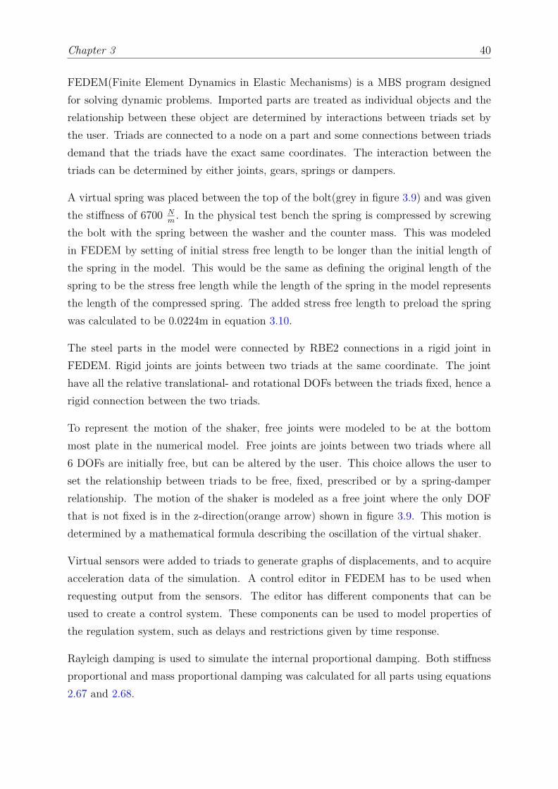
The rubber used in the test bench is vulcanized between two plates during production.When compressed or elongated along one axis it deforms by increasing or decreasing thecross section of the middle of the thickness of the rubber. Because the rubber is fixed inthe the x- and y-plane shown in figure 3.11, structural stiffness is added to the rubber.This means that the rubber 2.2 not only is dependent on the material stiffness shownin equation2.7. The stiffness of the rubber body is larger than what equation 2.7 wouldyield, since the equation does not consider structural stiffens. Two simulations using NXwere conducted to determine the added stiffness due to the transverse constraints of therubber.

Two simulations to investigate the added structural stiffness of the rubber due to thetransverse constraints were conducted. In the first simulation the rubber was fixed in thez-translation, but free to move in the x-y plane on the bottom and a load representedby pressure was added to the top. The pressure needed to deform the rubber 0.1mmwas calculated by using equation 2.8 and inserting material properties from table 3.5 andusing the cross section area from table 3.4. The equation with the values described aboveis shown in equation 3.13.

2.086 Nmm2 ∗ 0.0001m0.019m = 0.01098 N

mm2 (3.13)

The displacement resulting from the pressure in this case was 0.1mm as expected fromequation 3.13.

Chapter 3 42

Figure 3.10: Deformations from simulation in NX, fixed bottom and free displacementin x-y plane on top

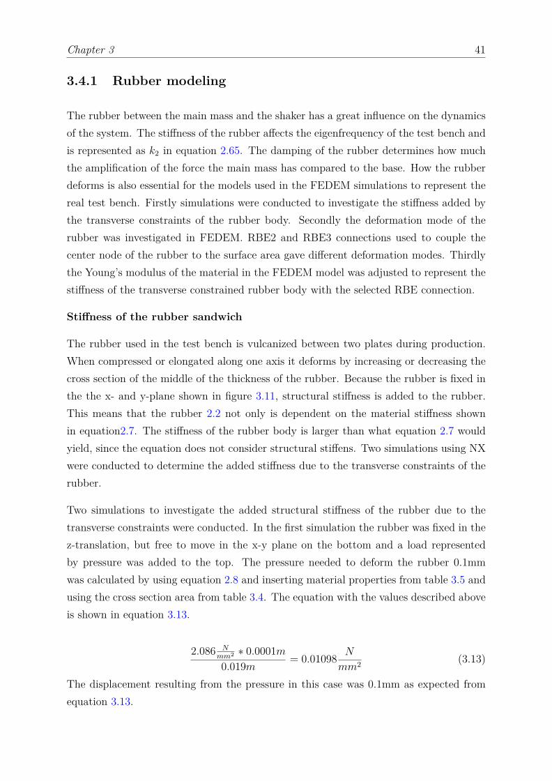
The second simulation was conducted while the bottom was fixed in all translations andthe cross section at the top was fixed in the x-y plane. This was done so that the simulatedrubber was constrained in a similar way like it would be in real life when it was vulcanisedto the rigid plates. The deformations from this simulation are shown in figure 3.11.

Figure 3.11: Deformations from simulation in NX, fixed bottom and fixed in x-yplane on top

Chapter 3 43

The simulated displacement in z-direction here was 0.0552mm compared to the 0.1mmin the first simulation. This will imply that the stiffness of the body is almost doubleddue to the added structural stiffness.

The stiffness of the rubber body was then calculated using the values found in the simu-lations. The total force on the body is 68.4N as shown in equation 3.14.

F = pA = 0.01098 N

mm2 ∗ 6233mm2 = 68.4N (3.14)

The stiffness of the rubber body can then be calculated by

k = F

δ= 68.4N

0.0000552m = 1239130Nm

(3.15)

This compared to the originally calculated stiffness of 670650 Nm

. This would result in anatural frequency of 136Hz by using equation 2.65. The stiffness found in equation 3.15was further used to adjust the Young’s modulus of the virtual rubber part exported tothe FEDEM simulation.

Deformation mode of the rubber sandwich

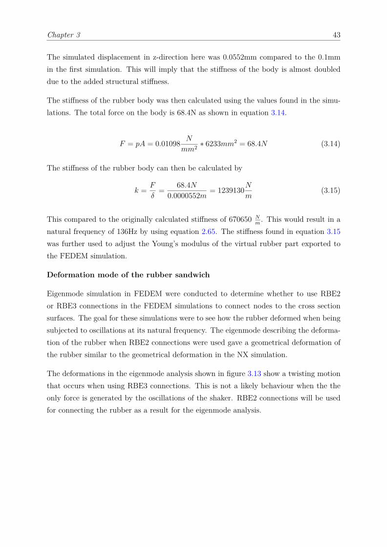
Eigenmode simulation in FEDEM were conducted to determine whether to use RBE2or RBE3 connections in the FEDEM simulations to connect nodes to the cross sectionsurfaces. The goal for these simulations were to see how the rubber deformed when beingsubjected to oscillations at its natural frequency. The eigenmode describing the deforma-tion of the rubber when RBE2 connections were used gave a geometrical deformation ofthe rubber similar to the geometrical deformation in the NX simulation.

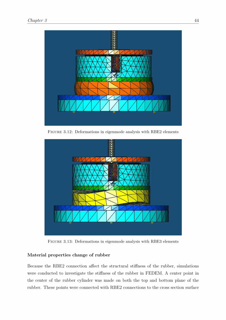
The deformations in the eigenmode analysis shown in figure 3.13 show a twisting motionthat occurs when using RBE3 connections. This is not a likely behaviour when the theonly force is generated by the oscillations of the shaker. RBE2 connections will be usedfor connecting the rubber as a result for the eigenmode analysis.

Chapter 3 44

Figure 3.12: Deformations in eigenmode analysis with RBE2 elements

Figure 3.13: Deformations in eigenmode analysis with RBE3 elements

Material properties change of rubber

Because the RBE2 connection affect the structural stiffness of the rubber, simulationswere conducted to investigate the stiffness of the rubber in FEDEM. A center point inthe center of the rubber cylinder was made on both the top and bottom plane of therubber. These points were connected with RBE2 connections to the cross section surface

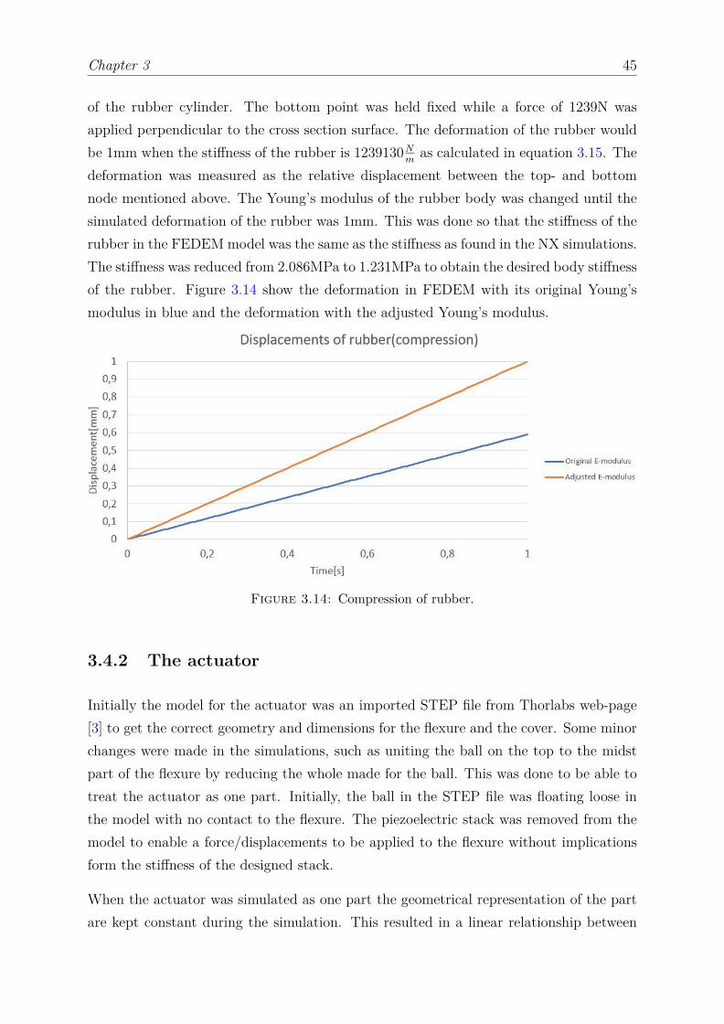
Chapter 3 45

of the rubber cylinder. The bottom point was held fixed while a force of 1239N wasapplied perpendicular to the cross section surface. The deformation of the rubber wouldbe 1mm when the stiffness of the rubber is 1239130N

mas calculated in equation 3.15. The

deformation was measured as the relative displacement between the top- and bottomnode mentioned above. The Young’s modulus of the rubber body was changed until thesimulated deformation of the rubber was 1mm. This was done so that the stiffness of therubber in the FEDEM model was the same as the stiffness as found in the NX simulations.The stiffness was reduced from 2.086MPa to 1.231MPa to obtain the desired body stiffnessof the rubber. Figure 3.14 show the deformation in FEDEM with its original Young’smodulus in blue and the deformation with the adjusted Young’s modulus.

Figure 3.14: Compression of rubber.

3.4.2 The actuator

Initially the model for the actuator was an imported STEP file from Thorlabs web-page[3] to get the correct geometry and dimensions for the flexure and the cover. Some minorchanges were made in the simulations, such as uniting the ball on the top to the midstpart of the flexure by reducing the whole made for the ball. This was done to be able totreat the actuator as one part. Initially, the ball in the STEP file was floating loose inthe model with no contact to the flexure. The piezoelectric stack was removed from themodel to enable a force/displacements to be applied to the flexure without implicationsform the stiffness of the designed stack.

When the actuator was simulated as one part the geometrical representation of the partare kept constant during the simulation. This resulted in a linear relationship between

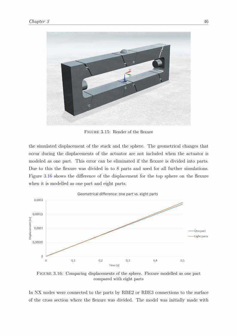
Chapter 3 46

Figure 3.15: Render of the flexure

the simulated displacement of the stack and the sphere. The geometrical changes thatoccur during the displacements of the actuator are not included when the actuator ismodeled as one part. This error can be eliminated if the flexure is divided into parts.Due to this the flexure was divided in to 8 parts and used for all further simulations.Figure 3.16 shows the difference of the displacement for the top sphere on the flexurewhen it is modelled as one part and eight parts.

Figure 3.16: Comparing displacements of the sphere. Flexure modelled as one partcompared with eight parts

In NX nodes were connected to the parts by RBE2 or RBE3 connections to the surfaceof the cross section where the flexure was divided. The model was initially made with

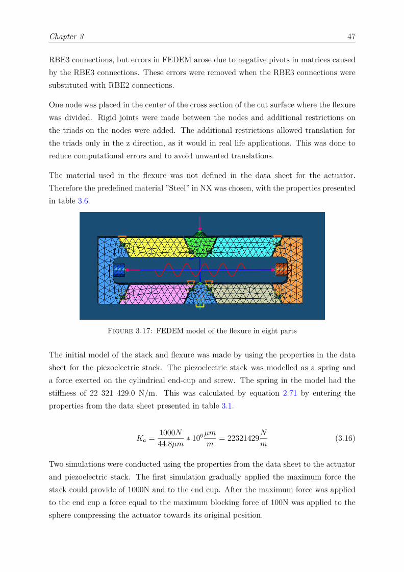
Chapter 3 47

RBE3 connections, but errors in FEDEM arose due to negative pivots in matrices causedby the RBE3 connections. These errors were removed when the RBE3 connections weresubstituted with RBE2 connections.

One node was placed in the center of the cross section of the cut surface where the flexurewas divided. Rigid joints were made between the nodes and additional restrictions onthe triads on the nodes were added. The additional restrictions allowed translation forthe triads only in the z direction, as it would in real life applications. This was done toreduce computational errors and to avoid unwanted translations.

The material used in the flexure was not defined in the data sheet for the actuator.Therefore the predefined material ”Steel” in NX was chosen, with the properties presentedin table 3.6.

Figure 3.17: FEDEM model of the flexure in eight parts

The initial model of the stack and flexure was made by using the properties in the datasheet for the piezoelectric stack. The piezoelectric stack was modelled as a spring anda force exerted on the cylindrical end-cup and screw. The spring in the model had thestiffness of 22 321 429.0 N/m. This was calculated by equation 2.71 by entering theproperties from the data sheet presented in table 3.1.

Ka = 1000N44.8µm ∗ 106µm

m= 22321429N

m(3.16)

Two simulations were conducted using the properties from the data sheet to the actuatorand piezoelectric stack. The first simulation gradually applied the maximum force thestack could provide of 1000N and to the end cup. After the maximum force was appliedto the end cup a force equal to the maximum blocking force of 100N was applied to thesphere compressing the actuator towards its original position.

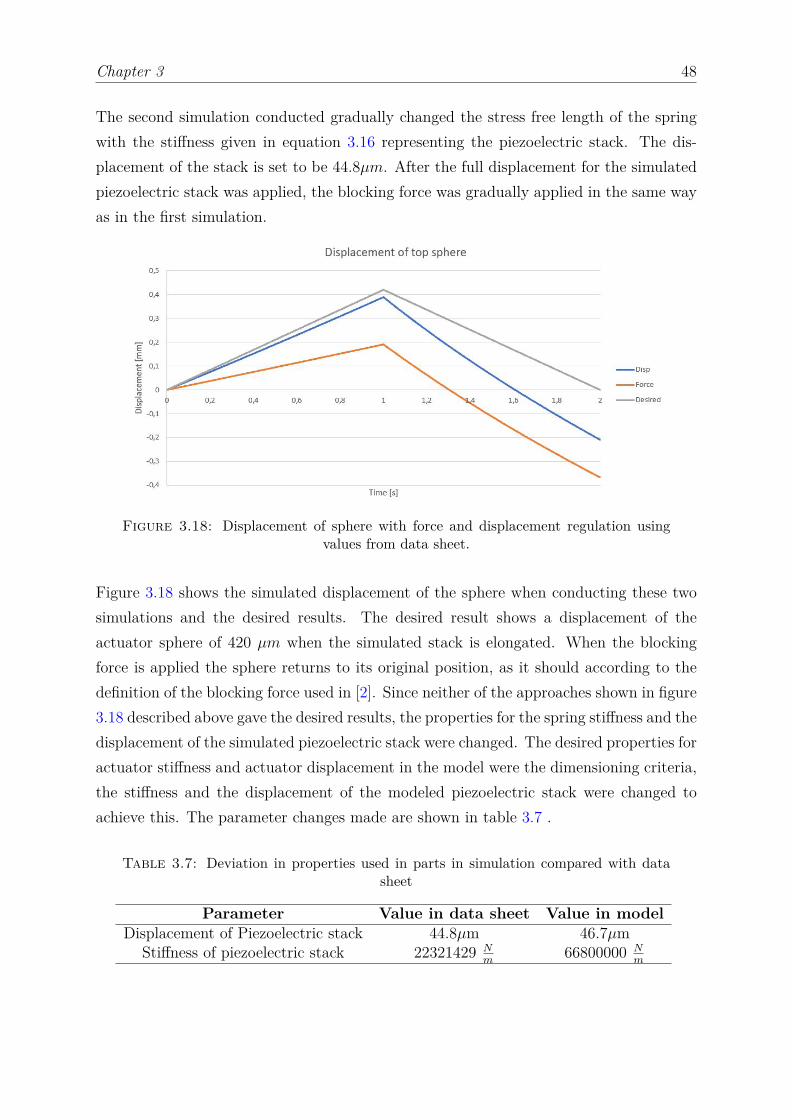
Chapter 3 48

The second simulation conducted gradually changed the stress free length of the springwith the stiffness given in equation 3.16 representing the piezoelectric stack. The dis-placement of the stack is set to be 44.8µm. After the full displacement for the simulatedpiezoelectric stack was applied, the blocking force was gradually applied in the same wayas in the first simulation.

Figure 3.18: Displacement of sphere with force and displacement regulation usingvalues from data sheet.

Figure 3.18 shows the simulated displacement of the sphere when conducting these twosimulations and the desired results. The desired result shows a displacement of theactuator sphere of 420 µm when the simulated stack is elongated. When the blockingforce is applied the sphere returns to its original position, as it should according to thedefinition of the blocking force used in [2]. Since neither of the approaches shown in figure3.18 described above gave the desired results, the properties for the spring stiffness and thedisplacement of the simulated piezoelectric stack were changed. The desired properties foractuator stiffness and actuator displacement in the model were the dimensioning criteria,the stiffness and the displacement of the modeled piezoelectric stack were changed toachieve this. The parameter changes made are shown in table 3.7 .

Table 3.7: Deviation in properties used in parts in simulation compared with datasheet

Parameter Value in data sheet Value in modelDisplacement of Piezoelectric stack 44.8µm 46.7µm

Stiffness of piezoelectric stack 22321429 Nm

66800000 Nm

Chapter 3 49

The relations of the stack displacement and the sphere displacement can be approximatedto be linear as shown in figure 3.16. By using the stack displacement value shown in table3.7 and remembering that the maximum displacement of the actuator is simulated to be420µm we can obtain the amplification factor, Af between the stack displacement andthe sphere displacement.

Af = 420µm46.7µm = 8.99 (3.17)

Chapter 4

Tests, calibrations and scripts

Several tests and were conducted to investigate how the coupling between the Arduinoand the accelerometer should be, how the Arduino should be programed, and how thesimulations should be adjusted to have dynamic properties that are similar to the physicaltest bench. A list over the tests and calibrating measures are listed below.

1. Noise in the circuit was measured with different hook up configurations betweenthe Arduino and other components to find the best configuration in section 4.1.

2. The time different commands in the scrips used were investigated to point out whatcommands to be avoided in the scripts in section 4.2.

3. Data from the accelerometers were investigated to find the relations between themeasured voltage and acceleration in section 4.3.

4. Scripts were developed and physical relations were investigated to be able to makea suitable way regulate the actuators in section 4.4.

5. Data from physical tests of the test bench using Vibration View and the shakerprovided by Teeness were conducted to adjust the properties in the simulations insection 4.5.

50

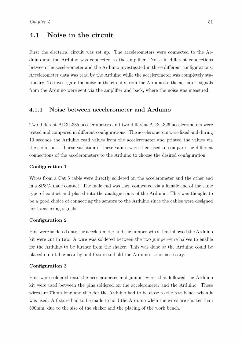
Chapter 4 51

4.1 Noise in the circuit

First the electrical circuit was set up. The accelerometers were connected to the Ar-duino and the Arduino was connected to the amplifier. Noise in different connectionsbetween the accelerometer and the Arduino investigated in three different configurations.Accelerometer data was read by the Arduino while the accelerometer was completely sta-tionary. To investigate the noise in the circuits from the Arduino to the actuator, signalsfrom the Arduino were sent via the amplifier and back, where the noise was measured.

4.1.1 Noise between accelerometer and Arduino

Two different ADXL335 accelerometers and two different ADXL326 accelerometers weretested and compared in different configurations. The accelerometers were fixed and during10 seconds the Arduino read values from the accelerometer and printed the values viathe serial port. These variation of these values were then used to compare the differentconnections of the accelerometers to the Arduino to choose the desired configuration.

Configuration 1

Wires from a Cat 5 cable were directly soldered on the accelerometer and the other endin a 8P8C- male contact. The male end was then connected via a female end of the sametype of contact and placed into the analogue pins of the Arduino. This was thought tobe a good choice of connecting the sensors to the Arduino since the cables were designedfor transferring signals.

Configuration 2

Pins were soldered onto the accelerometer and the jumper-wires that followed the Arduinokit were cut in two. A wire was soldered between the two jumper-wire halves to enablefor the Arduino to be further from the shaker. This was done so the Arduino could beplaced on a table near by and fixture to hold the Arduino is not necessary.

Configuration 3

Pins were soldered onto the accelerometer and jumper-wires that followed the Arduinokit were used between the pins soldered on the accelerometer and the Arduino. Thesewires are 70mm long and therefor the Arduino had to be close to the test bench when itwas used. A fixture had to be made to hold the Arduino when the wires are shorter than500mm, due to the size of the shaker and the placing of the work bench.

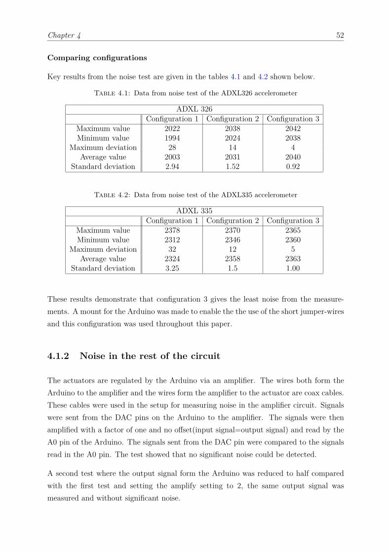
Chapter 4 52

Comparing configurations

Key results from the noise test are given in the tables 4.1 and 4.2 shown below.

Table 4.1: Data from noise test of the ADXL326 accelerometer

ADXL 326Configuration 1 Configuration 2 Configuration 3

Maximum value 2022 2038 2042Minimum value 1994 2024 2038

Maximum deviation 28 14 4Average value 2003 2031 2040

Standard deviation 2.94 1.52 0.92

Table 4.2: Data from noise test of the ADXL335 accelerometer

ADXL 335Configuration 1 Configuration 2 Configuration 3

Maximum value 2378 2370 2365Minimum value 2312 2346 2360

Maximum deviation 32 12 5Average value 2324 2358 2363

Standard deviation 3.25 1.5 1.00

These results demonstrate that configuration 3 gives the least noise from the measure-ments. A mount for the Arduino was made to enable the the use of the short jumper-wiresand this configuration was used throughout this paper.

4.1.2 Noise in the rest of the circuit

The actuators are regulated by the Arduino via an amplifier. The wires both form theArduino to the amplifier and the wires form the amplifier to the actuator are coax cables.These cables were used in the setup for measuring noise in the amplifier circuit. Signalswere sent from the DAC pins on the Arduino to the amplifier. The signals were thenamplified with a factor of one and no offset(input signal=output signal) and read by theA0 pin of the Arduino. The signals sent from the DAC pin were compared to the signalsread in the A0 pin. The test showed that no significant noise could be detected.

A second test where the output signal form the Arduino was reduced to half comparedwith the first test and setting the amplify setting to 2, the same output signal wasmeasured and without significant noise.

Chapter 4 53

4.2 Time used by functions in script

The speed of the code is important to ensure rapid output signals to generate smoothsignals at high frequencies. Therefore a script was run on the Arduino Due to measurethe time each instruction used in the script. This is done so that the speed of the scriptscan be improved and to investigate if there are some instructions in the code that shouldbe avoided due to time consumption. The script used to measure the time is shown infigure 4.1.

Figure 4.1: Script for measuring the time consumption for code instructions

The script outputs the number of rounds the loop can run within one second. The outputof the code was then used to calculate the time spent by each code by using equation 4.1.

Time used by instruction in µs = 1000000µsnumber of rounds (4.1)

The time used for some investigated codes are presented in table 4.3. When the loop ranwith no other function in it(NONE), the code spent 2µs. The ”Time added pr cycle”shows the time added as a result of including the function.

From this we can see that the Serial.print() command uses 83µs pr character sent via theserial communication. The analogRead()-values with a 12 bit resolution consist of up to4 characters leading to 83*4µs(332µs) spent for printing one output vale. For this reason

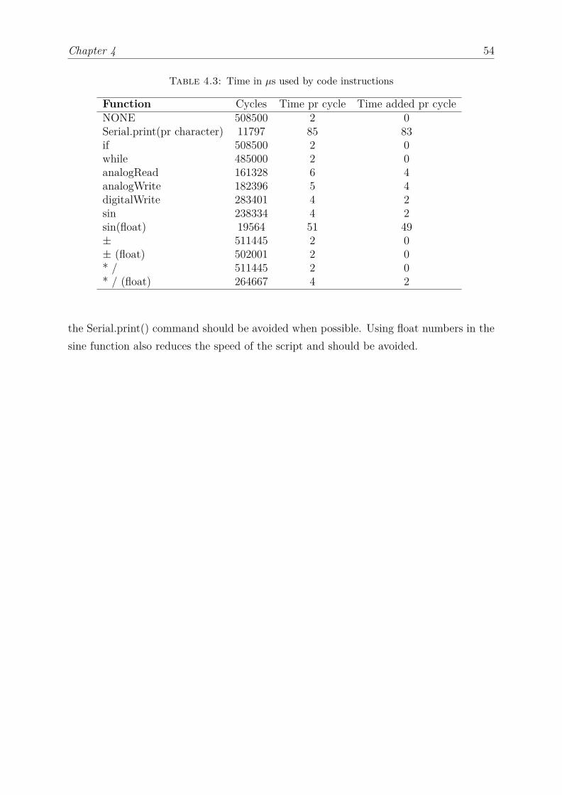
Chapter 4 54

Table 4.3: Time in µs used by code instructions

Function Cycles Time pr cycle Time added pr cycleNONE 508500 2 0Serial.print(pr character) 11797 85 83if 508500 2 0while 485000 2 0analogRead 161328 6 4analogWrite 182396 5 4digitalWrite 283401 4 2sin 238334 4 2sin(float) 19564 51 49± 511445 2 0± (float) 502001 2 0* / 511445 2 0* / (float) 264667 4 2

the Serial.print() command should be avoided when possible. Using float numbers in thesine function also reduces the speed of the script and should be avoided.

Chapter 4 55

4.3 Accelerometer

The accelerometers used are the ADXL335 and the ADXL326. The ADXL335 accelerom-eter is mounted on the main mass and the data from this accelerometer is used by theArduino to regulate the actuators. This makes the data form the ADXL335 imperativefor the regulation system. The ADXL326 accelerometer on the other hand is used usedto measure accelerations of the counter mass and not used for the regulation of the ac-tuators. Therefor the acceleration data from the main mass was deemed more importantthan the acceleration of the counter mass. Therefor the focus of the testing was on theADXL335 accelerometer.

A series of tests were conducted to investigate the performance of the ADXL335 ac-celerometer. Tests with frequencies ranging from 10Hz-150Hz and with 1, 2 and 3 timesthe acceleration of the gravity was applied to the accelerometer. A list of the tested pa-rameter combinations is shown in table 4.4. The accelerations and the frequencies wereinput in Vibration View and the Arduino compatible accelerometer was mounted on theshaker.

Table 4.4: Tests conducted to investigate accelerometer data precision

Acceleration Frequency1g 10 Hz1g 50 Hz1g 100 Hz1g 150 Hz2g 10 Hz2g 50 Hz2g 100 Hz2g 150 Hz3g 10 Hz3g 50 Hz3g 100 Hz3g 150 Hz

The raw data was logged for 10 seconds while the shaker applied the acceleration at thegiven frequency. The test at 10Hz giving an acceleration equal to 3 times of the gravity,could not be preformed because of a restriction of the translation length of the shaker.

The comparison of the values of the accelerometer output while varying the frequencyand acceleration was set to 1g is shown in figure 4.2. The graph shows that there is

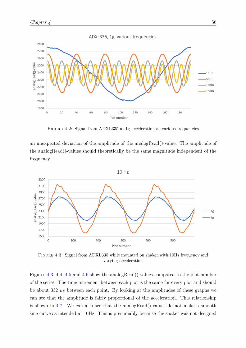
Chapter 4 56

Figure 4.2: Signal from ADXL335 at 1g acceleration at various frequencies

an unexpected deviation of the amplitude of the analogRead()-value. The amplitude ofthe analogRead()-values should theoretically be the same magnitude independent of thefrequency.

Figure 4.3: Signal from ADXL335 while mounted on shaker with 10Hz frequency andvarying acceleration

Figures 4.3, 4.4, 4.5 and 4.6 show the analogRead()-values compared to the plot numberof the series. The time increment between each plot is the same for every plot and shouldbe about 332 µs between each point. By looking at the amplitudes of these graphs wecan see that the amplitude is fairly proportional of the acceleration. This relationshipis shown in 4.7. We can also see that the analogRead()-values do not make a smoothsine curve as intended at 10Hz. This is presumably because the shaker was not designed

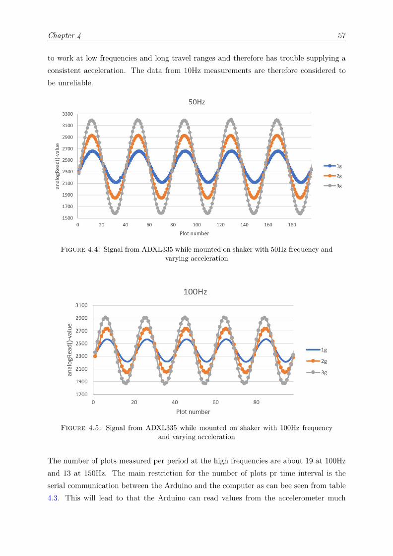
Chapter 4 57

to work at low frequencies and long travel ranges and therefore has trouble supplying aconsistent acceleration. The data from 10Hz measurements are therefore considered tobe unreliable.

Figure 4.4: Signal from ADXL335 while mounted on shaker with 50Hz frequency andvarying acceleration

Figure 4.5: Signal from ADXL335 while mounted on shaker with 100Hz frequencyand varying acceleration

The number of plots measured per period at the high frequencies are about 19 at 100Hzand 13 at 150Hz. The main restriction for the number of plots pr time interval is theserial communication between the Arduino and the computer as can bee seen from table4.3. This will lead to that the Arduino can read values from the accelerometer much

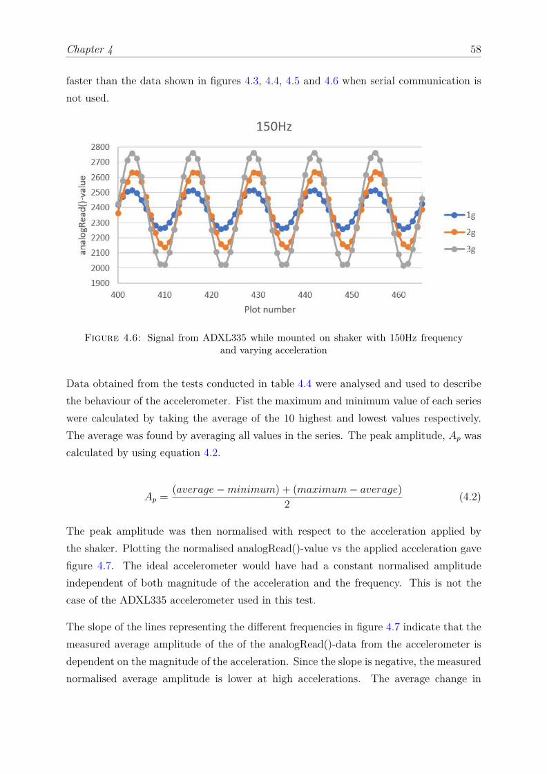
Chapter 4 58

faster than the data shown in figures 4.3, 4.4, 4.5 and 4.6 when serial communication isnot used.

Figure 4.6: Signal from ADXL335 while mounted on shaker with 150Hz frequencyand varying acceleration

Data obtained from the tests conducted in table 4.4 were analysed and used to describethe behaviour of the accelerometer. Fist the maximum and minimum value of each serieswere calculated by taking the average of the 10 highest and lowest values respectively.The average was found by averaging all values in the series. The peak amplitude, Ap wascalculated by using equation 4.2.

Ap = (average−minimum) + (maximum− average)2 (4.2)

The peak amplitude was then normalised with respect to the acceleration applied bythe shaker. Plotting the normalised analogRead()-value vs the applied acceleration gavefigure 4.7. The ideal accelerometer would have had a constant normalised amplitudeindependent of both magnitude of the acceleration and the frequency. This is not thecase of the ADXL335 accelerometer used in this test.

The slope of the lines representing the different frequencies in figure 4.7 indicate that themeasured average amplitude of the of the analogRead()-data from the accelerometer isdependent on the magnitude of the acceleration. Since the slope is negative, the measurednormalised average amplitude is lower at high accelerations. The average change in

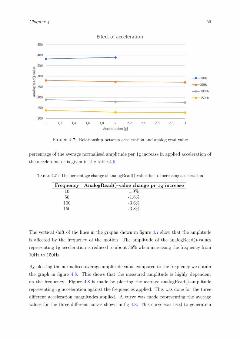
Chapter 4 59

Figure 4.7: Relationship between acceleration and analog read value

percentage of the average normalised amplitude per 1g increase in applied acceleration ofthe accelerometer is given in the table 4.5.

Table 4.5: The percentage change of analogRead()-value due to increasing acceleration

Frequency AnalogRead()-value change pr 1g increase10 1.9%50 -1.6%100 -3.6%150 -3.8%

The vertical shift of the lines in the graphs shown in figure 4.7 show that the amplitudeis affected by the frequency of the motion. The amplitude of the analogRead()-valuesrepresenting 1g acceleration is reduced to about 36% when increasing the frequency from10Hz to 150Hz.

By plotting the normalised average amplitude value compared to the frequency we obtainthe graph in figure 4.8. This shows that the measured amplitude is highly dependenton the frequency. Figure 4.8 is made by plotting the average analogRead()-amplituderepresenting 1g acceleration against the frequencies applied. This was done for the threedifferent acceleration magnitudes applied. A curve was made representing the averagevalues for the three different curves shown in fig 4.8. This curve was used to generate a

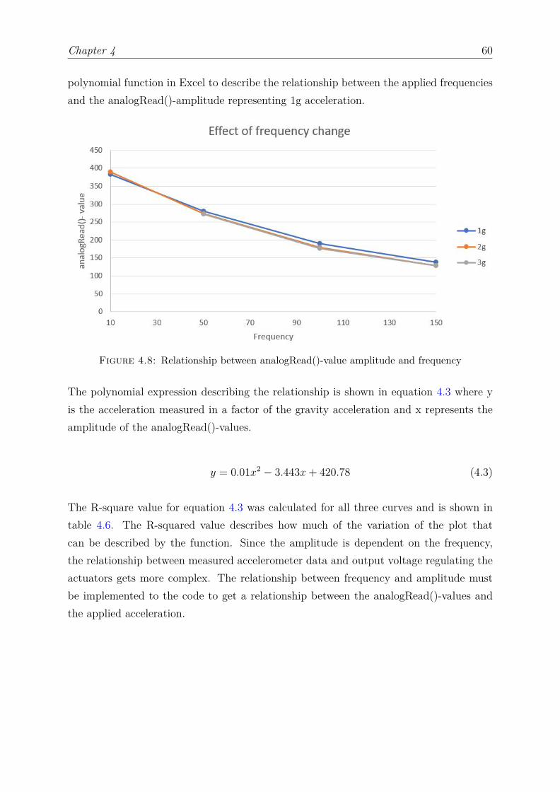
Chapter 4 60

polynomial function in Excel to describe the relationship between the applied frequenciesand the analogRead()-amplitude representing 1g acceleration.

Figure 4.8: Relationship between analogRead()-value amplitude and frequency

The polynomial expression describing the relationship is shown in equation 4.3 where yis the acceleration measured in a factor of the gravity acceleration and x represents theamplitude of the analogRead()-values.

y = 0.01x2 − 3.443x+ 420.78 (4.3)

The R-square value for equation 4.3 was calculated for all three curves and is shown intable 4.6. The R-squared value describes how much of the variation of the plot thatcan be described by the function. Since the amplitude is dependent on the frequency,the relationship between measured accelerometer data and output voltage regulating theactuators gets more complex. The relationship between frequency and amplitude mustbe implemented to the code to get a relationship between the analogRead()-values andthe applied acceleration.

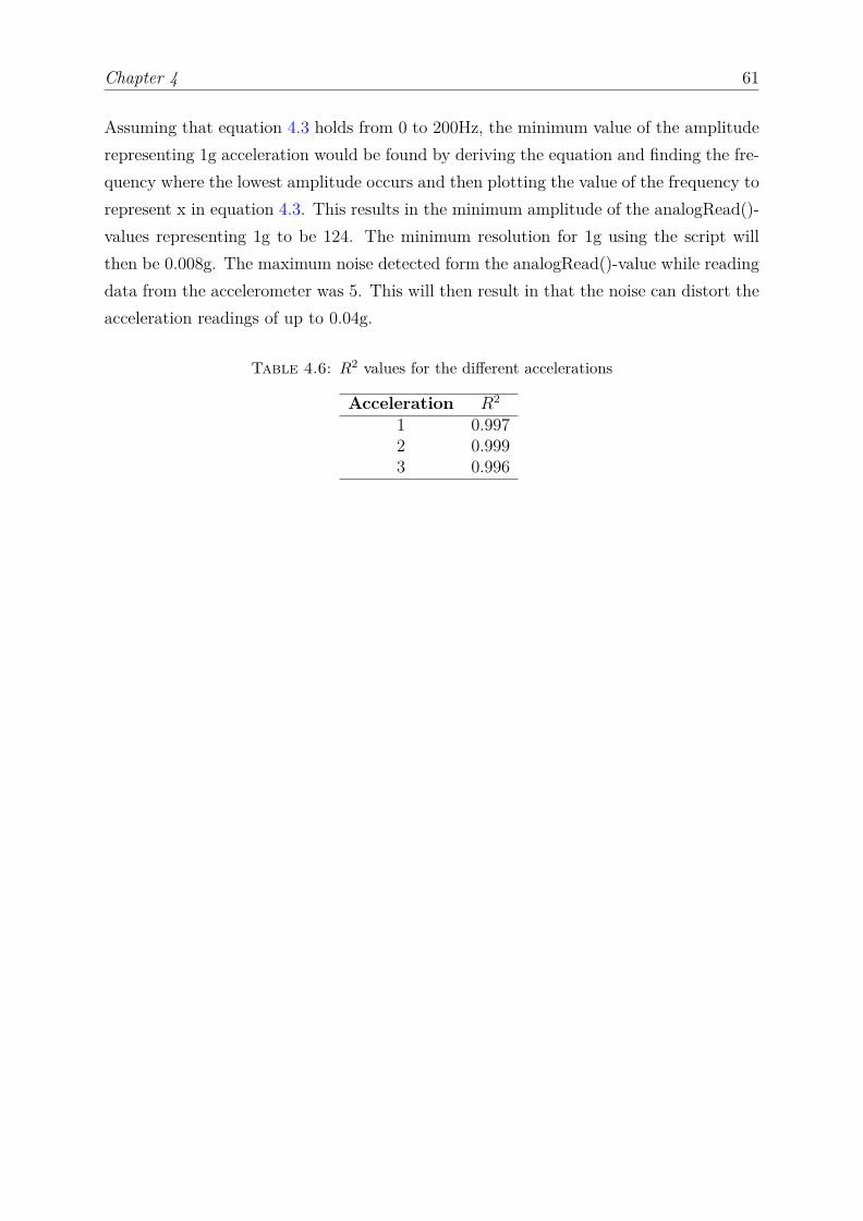
Chapter 4 61

Assuming that equation 4.3 holds from 0 to 200Hz, the minimum value of the amplituderepresenting 1g acceleration would be found by deriving the equation and finding the fre-quency where the lowest amplitude occurs and then plotting the value of the frequency torepresent x in equation 4.3. This results in the minimum amplitude of the analogRead()-values representing 1g to be 124. The minimum resolution for 1g using the script willthen be 0.008g. The maximum noise detected form the analogRead()-value while readingdata from the accelerometer was 5. This will then result in that the noise can distort theacceleration readings of up to 0.04g.

Table 4.6: R2 values for the different accelerations

Acceleration R2

1 0.9972 0.9993 0.996

Chapter 4 62

4.4 Scripts used in the Arduino Due

The signals from the accelerometers had to be treated to create an output from theArduino that regulates the actuators to dampen the vibrations. This was done by creatingscripts that interpret the accelerometer data to determine an output signal.

The amplitude, minimum, maximum and average of the analogRead()-values had to bemeasured and calculated to further be used to calculate the frequency of the input signal.These values were put in equation 4.3 to obtain the estimation of the acceleration. Therelationship between the output signal from the Arduino and the displacement of theactuator was calculated. The output signal algorithm has to be chosen and lastly a scriptto determine when to initiate the regulating signal in the desired phase was used.

The signal output from the Arduino is then sent via the amplifier to the actuator. It istherefor important that the signal from the Arduino is consistent and precise. Deviationsfrom the Arduino will also be amplified and will affect the regulation of the actuator andtherefor the damping properties of the active system.

4.4.1 Frequency and amplitude estimation

To be able to regulate the actuators with the correct signal, the data from the accelerome-ter had to be used to estimate the frequency and amplitude. The data has to be convertedto determine the amplitude and frequency of the motion of the accelerometer to be ableto generate the signal regulating the actuators. The Arduino must also be able to ensurethat the motion of the counter mass has the desired phase compared to the main mass.The script used for obtaining the frequency and amplitude follows the following steps:

1. Obtain minimum and maximum analogReadd()-values from the accelerometer.

2. Calculate the average analogRead()-value.

3. Measure time when the analogRead()-value is below average.

4. Measure time when the analogRead()-value is above average.

5. Calculate time of one cycle form time spent over and below the average.

6. Calculate frequency of cycle.

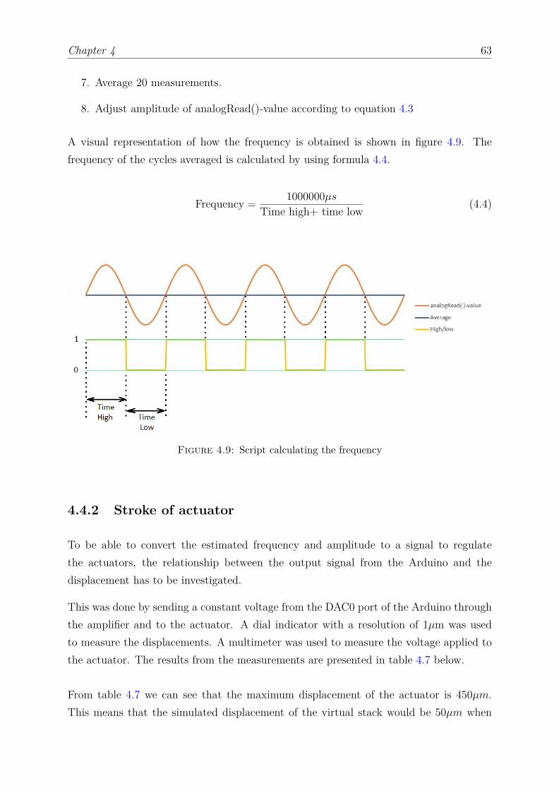
Chapter 4 63

7. Average 20 measurements.

8. Adjust amplitude of analogRead()-value according to equation 4.3

A visual representation of how the frequency is obtained is shown in figure 4.9. Thefrequency of the cycles averaged is calculated by using formula 4.4.

Frequency = 1000000µsTime high+ time low (4.4)

Figure 4.9: Script calculating the frequency

4.4.2 Stroke of actuator

To be able to convert the estimated frequency and amplitude to a signal to regulatethe actuators, the relationship between the output signal from the Arduino and thedisplacement has to be investigated.

This was done by sending a constant voltage from the DAC0 port of the Arduino throughthe amplifier and to the actuator. A dial indicator with a resolution of 1µm was usedto measure the displacements. A multimeter was used to measure the voltage applied tothe actuator. The results from the measurements are presented in table 4.7 below.

From table 4.7 we can see that the maximum displacement of the actuator is 450µm.This means that the simulated displacement of the virtual stack would be 50µm when

Chapter 4 64

Table 4.7: Applied voltage and corresponding displacement of actuators

Actuator 16.2V 33.5V 51.7V 71.0V1 98 µm 221 µm 350 µm 450 µm2 99 µm 224 µm 352 µm 453 µm3 98 µm 224 µm 351 µm 451 µm

dividing the measured maximum displacement with the amplification factor found inequation 3.17. This was implemented in the simulations by having a restriction of thepeak-to-peak amplitude of the simulated piezoelectric stack in the actuators to be 50µm.

Table 4.8: analogWrite()value, arduino voltage, amplified voltage

analogWrite()-value Arduino voltage output amplified voltage output0 0.55V 0.0V

1023 1.09V 16.2V2046 1.62V 33.5V3069 2.16V 51.7V4092 2.69V 71.0V

The relationship between the analogWrite()-values measured voltage from the Arduinoand measured voltage from the amplifier is shown in table 4.8. The graph in figure 4.10shows the relationship between the applied voltage an the displacement of the actuator.Using data from table 4.8 and table 4.7 a linear representation of the relationship betweenthe analogWrite()-values and the displacement of the actuator was calculated shown inequation 4.5.

Displacement of actuator = 0.105 analogWrite()-value (4.5)

4.4.3 Regulating output signal

A function to provide the desired output signal with amplitude and frequency estimatedin the scripts mentioned is needed to regulate the signal for the actuator. Two differentalgorithms to generate a sine signal were investigated and compared to choose the bestalgorithm.

ω t-sine function

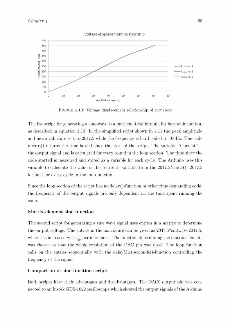
Chapter 4 65

Figure 4.10: Voltage displacement relationship of actuators

The fist script for generating a sine-wave is a mathematical formula for harmonic motion,as described in equation 2.13. In the simplified script shown in 4.11 the peak amplitudeand mean value are sett to 2047.5 while the frequency is hard coded to 100Hz. The codemicros() returns the time lapsed since the start of the script. The variable ”Current” isthe output signal and is calculated for every round in the loop section. The time since thecode started is measured and stored as a variable for each cycle. The Arduino uses thisvariable to calculate the value of the ”current”-variable from the 2047.5*sin(ωt)+2047.5formula for every cycle in the loop function.

Since the loop section of the script has no delay()-function or other time demanding code,the frequency of the output signals are only dependent on the time spent running thecode.

Matrix-element sine function

The second script for generating a sine wave signal uses entries in a matrix to determinethe output voltage. The entries in the matrix are can be given as 2047.5*sin(ωt)+2047.5,where t is increased with 1

50 per increment. The function determining the matrix elementswas chosen so that the whole resolution of the DAC pin was used. The loop functioncalls on the entries sequentially with the delayMicroseconds()-function controlling thefrequency of the signal.

Comparison of sine function scripts

Both scripts have their advantages and disadvantages. The DAC0 output pin was con-nected to an Instek GDS-1022 oscilloscope which showed the output signals of the Arduino

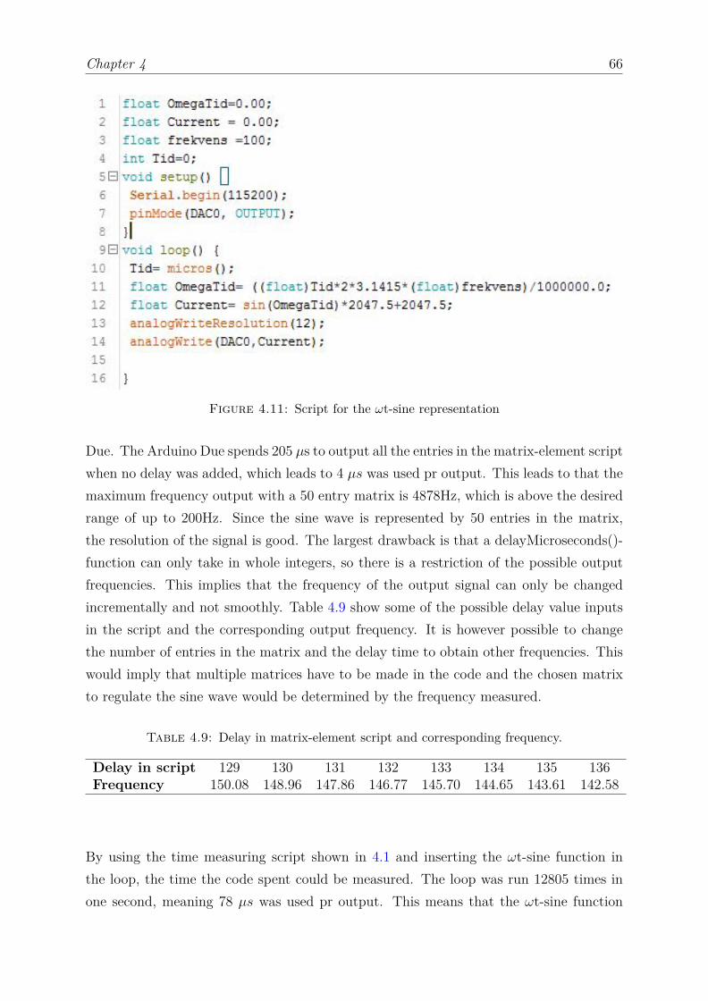
Chapter 4 66

Figure 4.11: Script for the ωt-sine representation

Due. The Arduino Due spends 205 µs to output all the entries in the matrix-element scriptwhen no delay was added, which leads to 4 µs was used pr output. This leads to that themaximum frequency output with a 50 entry matrix is 4878Hz, which is above the desiredrange of up to 200Hz. Since the sine wave is represented by 50 entries in the matrix,the resolution of the signal is good. The largest drawback is that a delayMicroseconds()-function can only take in whole integers, so there is a restriction of the possible outputfrequencies. This implies that the frequency of the output signal can only be changedincrementally and not smoothly. Table 4.9 show some of the possible delay value inputsin the script and the corresponding output frequency. It is however possible to changethe number of entries in the matrix and the delay time to obtain other frequencies. Thiswould imply that multiple matrices have to be made in the code and the chosen matrixto regulate the sine wave would be determined by the frequency measured.

Table 4.9: Delay in matrix-element script and corresponding frequency.

Delay in script 129 130 131 132 133 134 135 136Frequency 150.08 148.96 147.86 146.77 145.70 144.65 143.61 142.58

By using the time measuring script shown in 4.1 and inserting the ωt-sine function inthe loop, the time the code spent could be measured. The loop was run 12805 times inone second, meaning 78 µs was used pr output. This means that the ωt-sine function

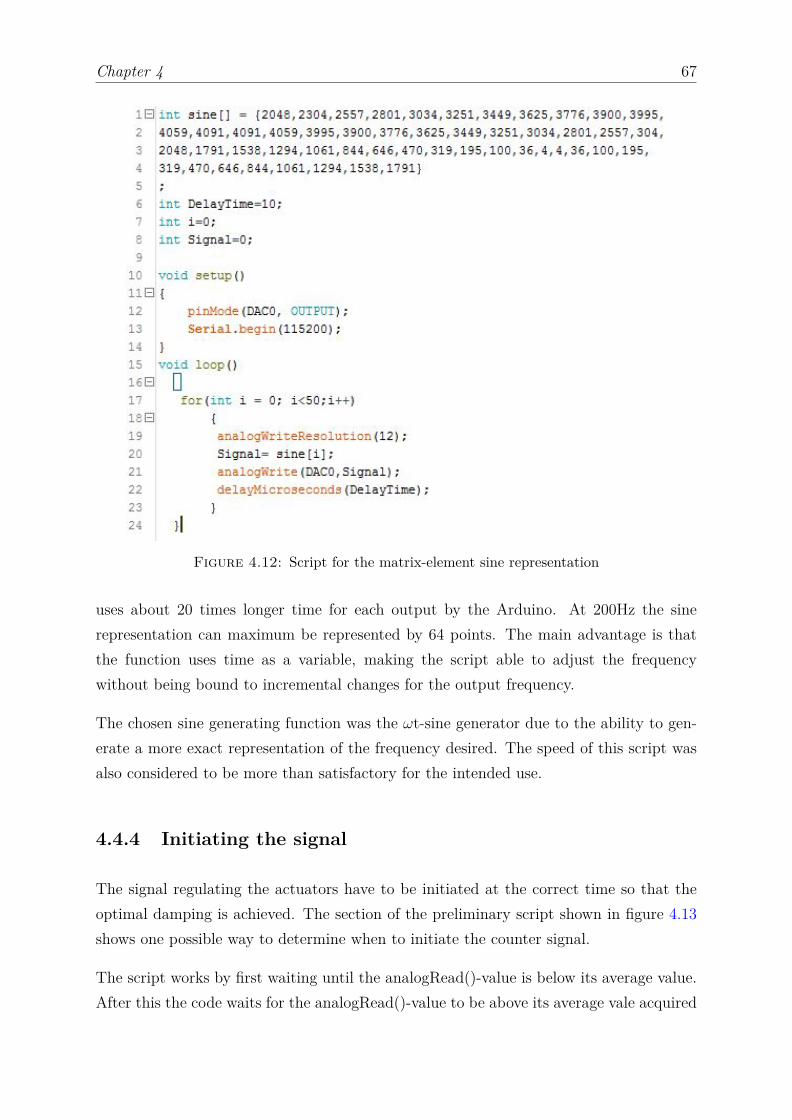
Chapter 4 67

Figure 4.12: Script for the matrix-element sine representation

uses about 20 times longer time for each output by the Arduino. At 200Hz the sinerepresentation can maximum be represented by 64 points. The main advantage is thatthe function uses time as a variable, making the script able to adjust the frequencywithout being bound to incremental changes for the output frequency.

The chosen sine generating function was the ωt-sine generator due to the ability to gen-erate a more exact representation of the frequency desired. The speed of this script wasalso considered to be more than satisfactory for the intended use.

4.4.4 Initiating the signal

The signal regulating the actuators have to be initiated at the correct time so that theoptimal damping is achieved. The section of the preliminary script shown in figure 4.13shows one possible way to determine when to initiate the counter signal.

The script works by first waiting until the analogRead()-value is below its average value.After this the code waits for the analogRead()-value to be above its average vale acquired

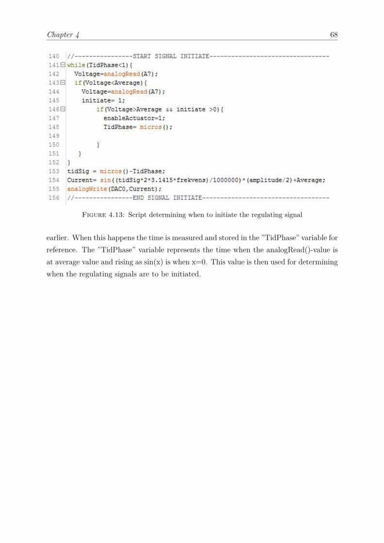
Chapter 4 68

Figure 4.13: Script determining when to initiate the regulating signal

earlier. When this happens the time is measured and stored in the ”TidPhase” variable forreference. The ”TidPhase” variable represents the time when the analogRead()-value isat average value and rising as sin(x) is when x=0. This value is then used for determiningwhen the regulating signals are to be initiated.

Chapter 4 69

4.5 Adjusting properties in the simulations

Firstly a sweep test of the whole test bench was conducted to compare the simulated re-sults with the measured results using Vibration View and the ”Data Physics V350/DSA1-1k” shaker. The sensors, software and the shaker provided by Teeness are assumed to betuned correctly and will be used as reference for calibrating the Arduino components.

A physical sine sweep test with the shaker and Vibration View was conducted fist with thestructure while the counter mass, bolt, washer and spring were removed. This was doneto compare the behaviour of the real life test bench with the simulated test bench beforeadding the counterweight. This was partly done because the modeling of the actuatorscould be a source of error and partly because the modeling of the rubber could be a sourceof error.

A physical test using the shaker to oscillate in a motion described by a sine wave with anincreasing frequency from 20Hz to 250Hz. The a maximum absolute peak acceleration wasset to 0.1g. Figure 4.14 shows the graph in dark blue(Ch2) representing the accelerationof the main mass as a function of frequency. The maximum acceleration was measured tobe 1.7g at 178Hz. This is an amplification of 17 compared to the acceleration regulatedby the shaker. By considering equation 2.45 the amplification factor of 17 would indicatea damping ration of the rubber to be slightly below 3%. The green line show the appliedacceleration by the shaker and light blue line show the measured acceleration of the base.The red lines show half/double of the demand output and the yellow striped lines showthe 50% increase/decrees of the demand acceleration.

Figure 4.14: Results from Vibration View, frequency sweep at 0.1g acceleration with-out damping components

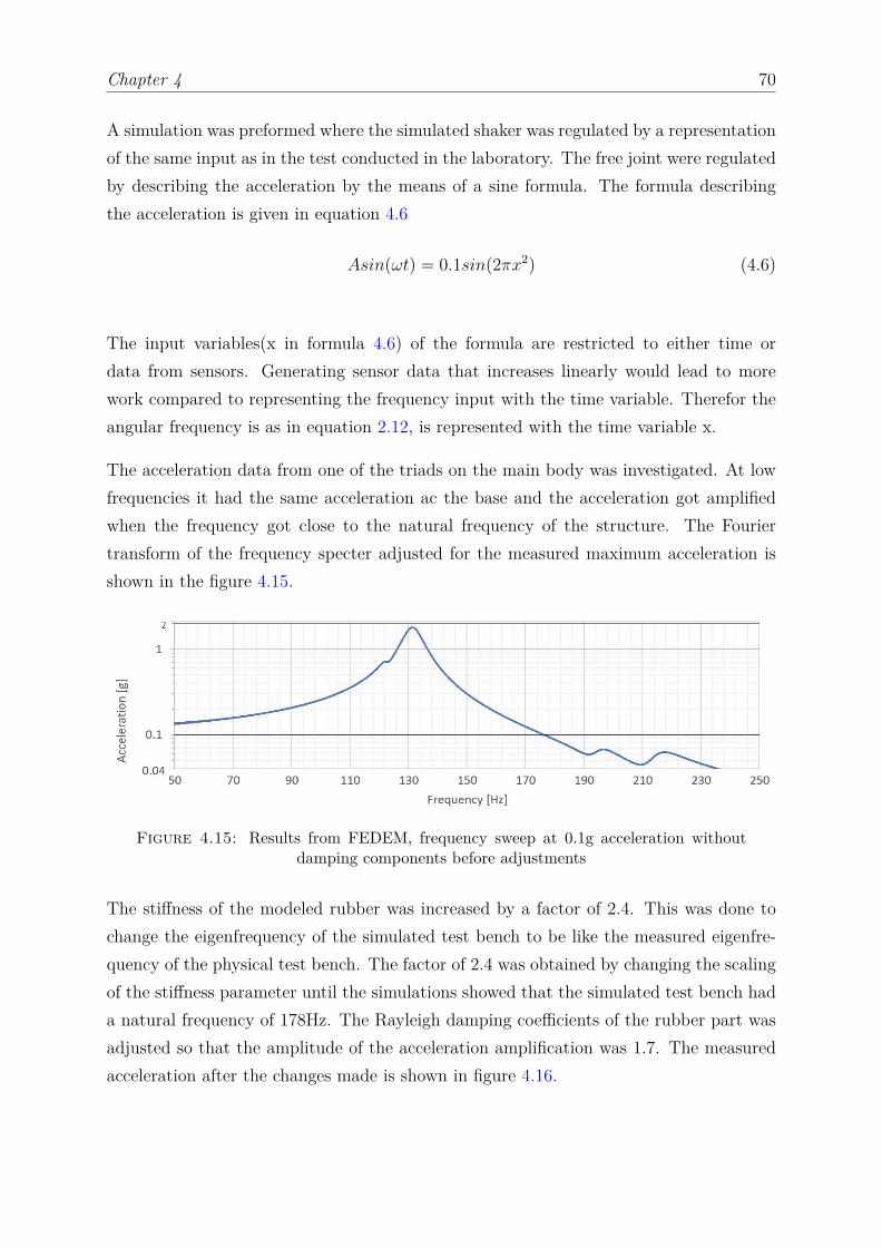
Chapter 4 70

A simulation was preformed where the simulated shaker was regulated by a representationof the same input as in the test conducted in the laboratory. The free joint were regulatedby describing the acceleration by the means of a sine formula. The formula describingthe acceleration is given in equation 4.6

Asin(ωt) = 0.1sin(2πx2) (4.6)

The input variables(x in formula 4.6) of the formula are restricted to either time ordata from sensors. Generating sensor data that increases linearly would lead to morework compared to representing the frequency input with the time variable. Therefor theangular frequency is as in equation 2.12, is represented with the time variable x.

The acceleration data from one of the triads on the main body was investigated. At lowfrequencies it had the same acceleration ac the base and the acceleration got amplifiedwhen the frequency got close to the natural frequency of the structure. The Fouriertransform of the frequency specter adjusted for the measured maximum acceleration isshown in the figure 4.15.

Figure 4.15: Results from FEDEM, frequency sweep at 0.1g acceleration withoutdamping components before adjustments

The stiffness of the modeled rubber was increased by a factor of 2.4. This was done tochange the eigenfrequency of the simulated test bench to be like the measured eigenfre-quency of the physical test bench. The factor of 2.4 was obtained by changing the scalingof the stiffness parameter until the simulations showed that the simulated test bench hada natural frequency of 178Hz. The Rayleigh damping coefficients of the rubber part wasadjusted so that the amplitude of the acceleration amplification was 1.7. The measuredacceleration after the changes made is shown in figure 4.16.

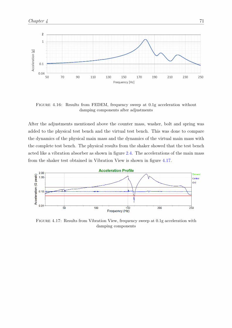
Chapter 4 71

Figure 4.16: Results from FEDEM, frequency sweep at 0.1g acceleration withoutdamping components after adjustments

After the adjustments mentioned above the counter mass, washer, bolt and spring wasadded to the physical test bench and the virtual test bench. This was done to comparethe dynamics of the physical main mass and the dynamics of the virtual main mass withthe complete test bench. The physical results from the shaker showed that the test benchacted like a vibration absorber as shown in figure 2.4. The accelerations of the main massfrom the shaker test obtained in Vibration View is shown in figure 4.17.

Figure 4.17: Results from Vibration View, frequency sweep at 0.1g acceleration withdamping components

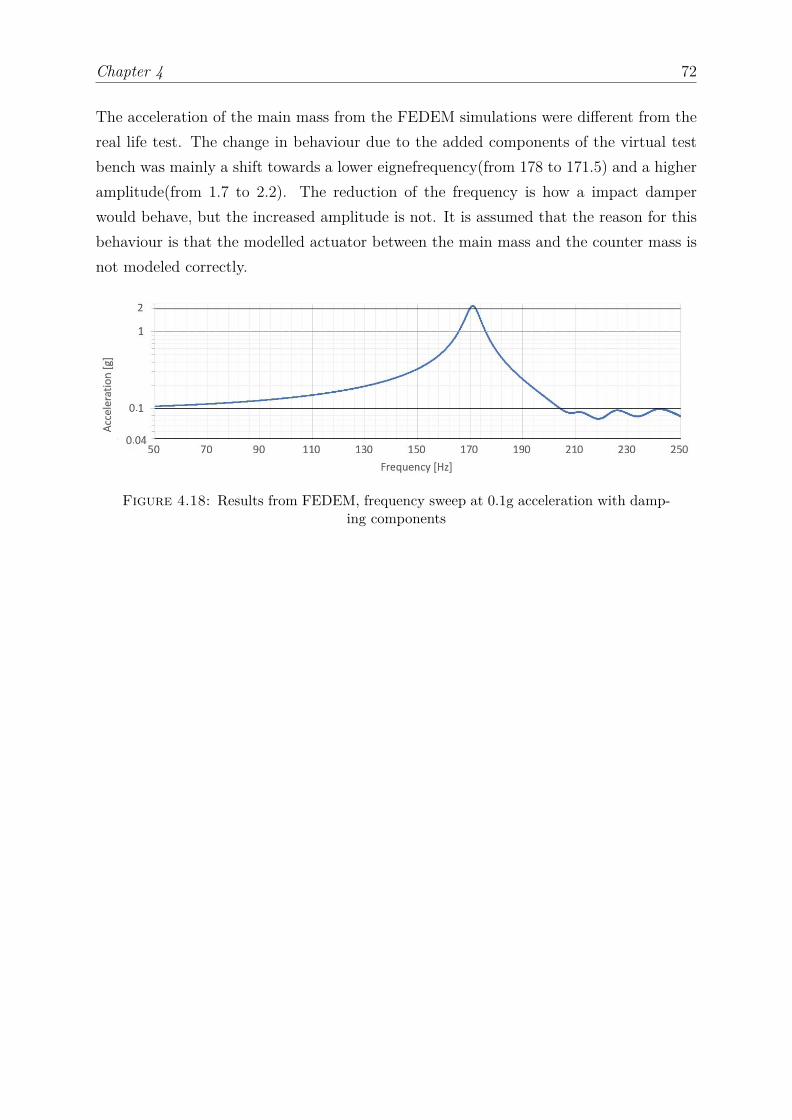
Chapter 4 72

The acceleration of the main mass from the FEDEM simulations were different from thereal life test. The change in behaviour due to the added components of the virtual testbench was mainly a shift towards a lower eignefrequency(from 178 to 171.5) and a higheramplitude(from 1.7 to 2.2). The reduction of the frequency is how a impact damperwould behave, but the increased amplitude is not. It is assumed that the reason for thisbehaviour is that the modelled actuator between the main mass and the counter mass isnot modeled correctly.

Figure 4.18: Results from FEDEM, frequency sweep at 0.1g acceleration with damp-ing components

Chapter 5

Results

Several simulations were preformed to investigate the dynamics of the virtual test benchand how the actuators should be regulated to reduce the vibrations of the main mass.Further tests were conducted to measure the error of the Arduino readings and calcu-lations. These results were used to evaluate if the Arduino is suited for regulating theactive damping system.

5.1 Active damping simulations

The goal of these simulations were to investigate how to dampen the vibrations of the mainmass. The effect of deviations in both amplitude and frequencies were also investigated.

In these simulations the simulated base excitation had a constant frequency of 140Hzwas chosen as reference while the acceleration was set to 5m

s2 unless otherwise is specified.The frequency was chosen because it is a high frequency far from the natural frequency,making it a suited reference frequencies for general behaviour of the virtual test bench.The low value of the acceleration was due to the restrictions of the actuators. Also in reallife testing of the test bench it is preferable to start with low forces for safety reasons. Thefree joins representing the shaker were regulated by displacements. The values describingthe displacement of the shaker is given in table 5.1

The amplitude of the motion of the free joints was calculated by choosing the desiredacceleration to be 5m

s2 and rearranging equation 2.15. The simulated displacement of thevirtual main mass was obtained during the simulation when the displacement change of

73

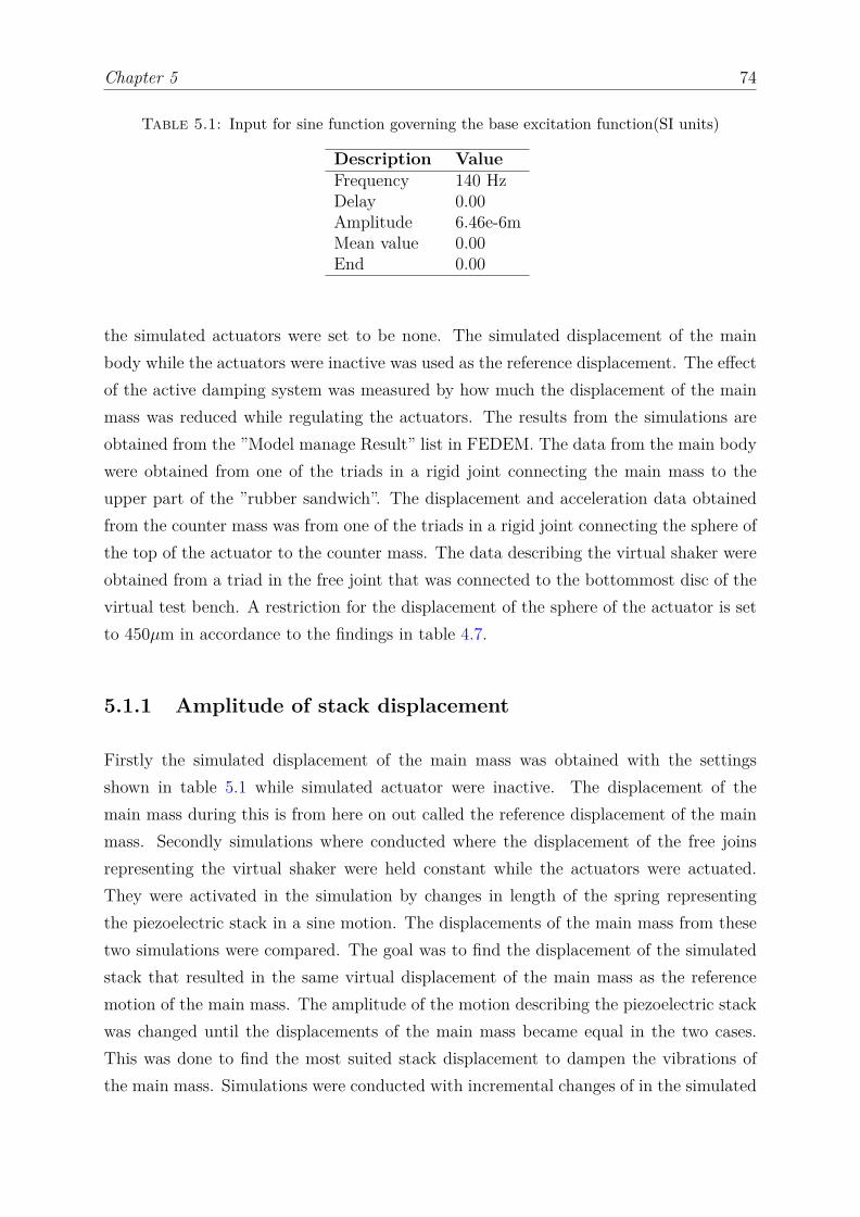
Chapter 5 74

Table 5.1: Input for sine function governing the base excitation function(SI units)

Description ValueFrequency 140 HzDelay 0.00Amplitude 6.46e-6mMean value 0.00End 0.00

the simulated actuators were set to be none. The simulated displacement of the mainbody while the actuators were inactive was used as the reference displacement. The effectof the active damping system was measured by how much the displacement of the mainmass was reduced while regulating the actuators. The results from the simulations areobtained from the ”Model manage Result” list in FEDEM. The data from the main bodywere obtained from one of the triads in a rigid joint connecting the main mass to theupper part of the ”rubber sandwich”. The displacement and acceleration data obtainedfrom the counter mass was from one of the triads in a rigid joint connecting the sphere ofthe top of the actuator to the counter mass. The data describing the virtual shaker wereobtained from a triad in the free joint that was connected to the bottommost disc of thevirtual test bench. A restriction for the displacement of the sphere of the actuator is setto 450µm in accordance to the findings in table 4.7.

5.1.1 Amplitude of stack displacement

Firstly the simulated displacement of the main mass was obtained with the settingsshown in table 5.1 while simulated actuator were inactive. The displacement of themain mass during this is from here on out called the reference displacement of the mainmass. Secondly simulations where conducted where the displacement of the free joinsrepresenting the virtual shaker were held constant while the actuators were actuated.They were activated in the simulation by changes in length of the spring representingthe piezoelectric stack in a sine motion. The displacements of the main mass from thesetwo simulations were compared. The goal was to find the displacement of the simulatedstack that resulted in the same virtual displacement of the main mass as the referencemotion of the main mass. The amplitude of the motion describing the piezoelectric stackwas changed until the displacements of the main mass became equal in the two cases.This was done to find the most suited stack displacement to dampen the vibrations ofthe main mass. Simulations were conducted with incremental changes of in the simulated

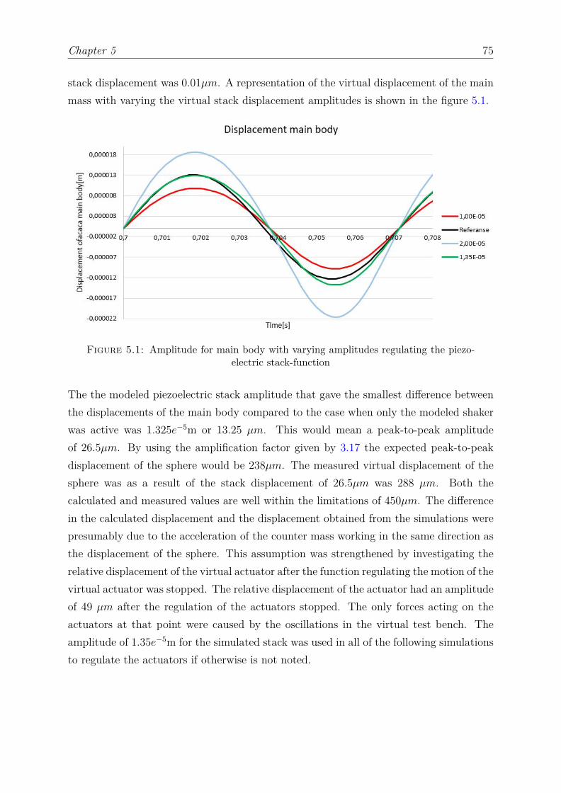
Chapter 5 75

stack displacement was 0.01µm. A representation of the virtual displacement of the mainmass with varying the virtual stack displacement amplitudes is shown in the figure 5.1.

Figure 5.1: Amplitude for main body with varying amplitudes regulating the piezo-electric stack-function

The the modeled piezoelectric stack amplitude that gave the smallest difference betweenthe displacements of the main body compared to the case when only the modeled shakerwas active was 1.325e−5m or 13.25 µm. This would mean a peak-to-peak amplitudeof 26.5µm. By using the amplification factor given by 3.17 the expected peak-to-peakdisplacement of the sphere would be 238µm. The measured virtual displacement of thesphere was as a result of the stack displacement of 26.5µm was 288 µm. Both thecalculated and measured values are well within the limitations of 450µm. The differencein the calculated displacement and the displacement obtained from the simulations werepresumably due to the acceleration of the counter mass working in the same direction asthe displacement of the sphere. This assumption was strengthened by investigating therelative displacement of the virtual actuator after the function regulating the motion of thevirtual actuator was stopped. The relative displacement of the actuator had an amplitudeof 49 µm after the regulation of the actuators stopped. The only forces acting on theactuators at that point were caused by the oscillations in the virtual test bench. Theamplitude of 1.35e−5m for the simulated stack was used in all of the following simulationsto regulate the actuators if otherwise is not noted.

Chapter 5 76

5.1.2 Phase specter resulting in vibration reduction

If the relative displacement of the actuator work in the same direction as the displace-ment of the shaker simultaneously, the resulting displacement of the main mass would beamplified as a result for the actuation of the actuators. This would result in the displace-ment of the main mass getting a constructive interference, increasing the displacementof the main mass. To reduce the vibrations of the main mass a phase shift is applied tothe function representing the piezoelectric stack. This is done so that the displacementsby the main mass caused by the actuators work against the displacements caused by theshaker.

To investigate how the phase delay of the function regulating the actuators affects thedisplacement of the main body several simulations were conducted. Fist simulations witha phase delay fraction of a period varying from 0.0 to 1.0 were conducted with 0.1 fractionof a period as increment. Later simulations with 0.01 increment of fraction of period wereconducted near the phases where the maximum reduction of vibrations were achieved andwhere the effect of the vibration reduction got near none. A representation of the delayin the function regulating the actuators versus the amplification of the amplitude to thedisplacement of the main mass is show in figure 5.2.

Figure 5.2: Fraction of phase vs. amplification of vibrations

The graph shows that at a delay of a 0.49 phase reduces the amplitude of the vibrationsof the main mass about 90%. Further the graph shows that when the delay is between

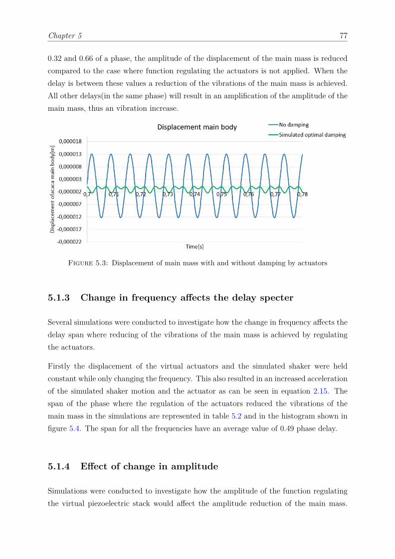
Chapter 5 77

0.32 and 0.66 of a phase, the amplitude of the displacement of the main mass is reducedcompared to the case where function regulating the actuators is not applied. When thedelay is between these values a reduction of the vibrations of the main mass is achieved.All other delays(in the same phase) will result in an amplification of the amplitude of themain mass, thus an vibration increase.

Figure 5.3: Displacement of main mass with and without damping by actuators

5.1.3 Change in frequency affects the delay specter

Several simulations were conducted to investigate how the change in frequency affects thedelay span where reducing of the vibrations of the main mass is achieved by regulatingthe actuators.

Firstly the displacement of the virtual actuators and the simulated shaker were heldconstant while only changing the frequency. This also resulted in an increased accelerationof the simulated shaker motion and the actuator as can be seen in equation 2.15. Thespan of the phase where the regulation of the actuators reduced the vibrations of themain mass in the simulations are represented in table 5.2 and in the histogram shown infigure 5.4. The span for all the frequencies have an average value of 0.49 phase delay.

5.1.4 Effect of change in amplitude

Simulations were conducted to investigate how the amplitude of the function regulatingthe virtual piezoelectric stack would affect the amplitude reduction of the main mass.

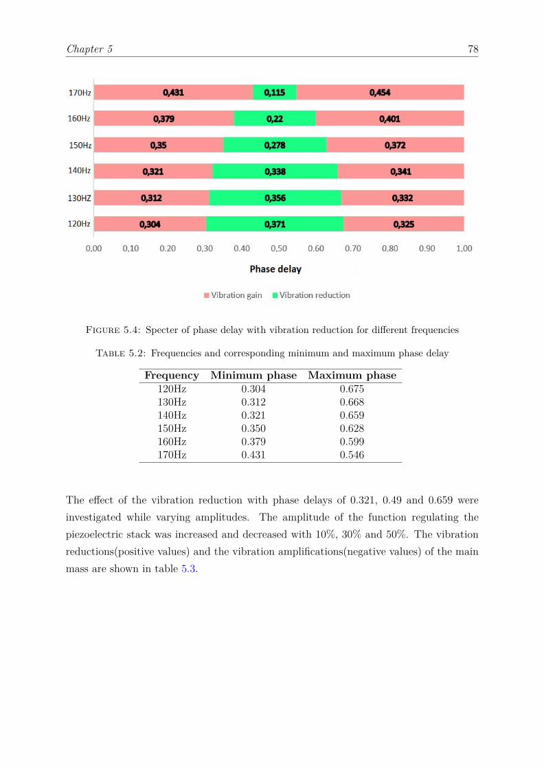
Chapter 5 78

Figure 5.4: Specter of phase delay with vibration reduction for different frequencies

Table 5.2: Frequencies and corresponding minimum and maximum phase delay

Frequency Minimum phase Maximum phase120Hz 0.304 0.675130Hz 0.312 0.668140Hz 0.321 0.659150Hz 0.350 0.628160Hz 0.379 0.599170Hz 0.431 0.546

The effect of the vibration reduction with phase delays of 0.321, 0.49 and 0.659 wereinvestigated while varying amplitudes. The amplitude of the function regulating thepiezoelectric stack was increased and decreased with 10%, 30% and 50%. The vibrationreductions(positive values) and the vibration amplifications(negative values) of the mainmass are shown in table 5.3.

Chapter 5 79

Table 5.3: Reduction(negative values) and gain(positive values) of displacement am-plitude

Amplitude 0.49 Phase delaydamping 0.321 Phase delay 0.659 Phase delay6.750e−6 54.7% 16.9% 17.0%8.508e−6 67.9% 15.3% 15.4%1.215e−5 89.5% 5.6% 5.5%1.325e−5 90.1% -0.1% -0.1%1.485e−5 81.4% -6.6% -6.6%1.755e−5 61.2% -21.7% -21.5%2.025e−5 39.7% -38.9% -38.5%

5.2 Active damping regulation

The main goal for this section is to investigate the scripts used for reading data from theaccelerometers and how the data is treated.

5.2.1 Measurement of frequencies

Errors in the frequency estimations may occur, when measuring the frequency of theoscillations of the main body form the accelerometer with the Arduino. The small de-viation between the real frequency of the main body and the applied control signal tothe actuators will over time result in a phase shift between the signals. Assuming thata script similar to the script described in section 4.4.1 can be modified to read the errorand adjust the control signal regulating the actuators an estimation of the allowed errorcan be made. The script uses 20 oscillations to determine the frequency. In calculatingthe allowed frequency error some assumptions have to be made.

1. There are 20 oscillations between every time the frequency can be changed by theArduino.

2. The script regulating the frequencies shifts the frequency to obtain a phase that iscloser to the optimal damping phase.

3. The first phase delay is exact, only the frequency is wrong.

4. The amplitude of the displacement of the main body should not be increased.

5. The time the Arduino needs to do calculations is during the sampling time.

Chapter 5 80

In the case where the frequency is 140Hz and the amplitude of the stack regulatingfunction is 13.25µm the allowed error is 0.00845, calculated from equation 5.1. If theerror is larger than this then the phase shift after 20 oscillations will be outside the phasespan where teh vibrations of the main mass are reduced, shown in figure 5.2. This willresult in that the amplitude of the displacement of main mass will be amplified in thelast oscillations before the regulating script can adjust the error.

Maximum frequency error = positive delay specter2 ∗ oscillations in one set = 0.338

2 ∗ 20 = 0.00845 (5.1)

This gives a maximum tolerated error of of 0.06% on the frequency estimation at 140Hz.

5.2.2 Reading the frequency with Arduino

The Arduino was hooked up to an oscilloscope to investigate how precise the scriptcould estimate the frequency. The oscilloscope is assumed to be perfect and thereforeall deviations from the applied frequency to the estimated frequency of the Arduino areexplained by error in the code or the Arduino.

The error from the measurements by the Arduino vs. the frequency is plotted in figure 5.5.40 reading samples for the frequency measurements were used to calculate the maximumerror and the standard deviation error. The plotted maximum allowed error is calculatedfor 120Hz to 170Hz by using equation 5.1. For the frequencies below 120Hz, the increasein allowed error was estimated by using the increase of allowed error found in the lowestthree measured frequencies. This will not give exact values, but it may give an indicationof the measured errors and the maximum errors allowed.

5.2.3 Calculating the acceleration with Arduino

The ADXL335 accelerometer was mounted on a disc that was fastened to the shaker.The shaker was set to generate a motion with the frequencies 50Hz, 100Hz and 150Hz atdifferent accelerations. The script first estimated the frequency and then estimated theacceleration of the accelerometer. The results from the test is shown in table 5.4.

The script is sensitive to noise, because it uses the extreme values to determine the spanof the analogRead()-values. These values are then used to determine the acceleration of

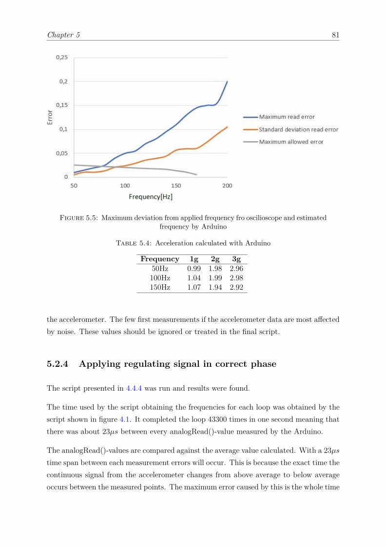
Chapter 5 81

Figure 5.5: Maximum deviation from applied frequency fro oscilioscope and estimatedfrequency by Arduino

Table 5.4: Acceleration calculated with Arduino

Frequency 1g 2g 3g50Hz 0.99 1.98 2.96100Hz 1.04 1.99 2.98150Hz 1.07 1.94 2.92

the accelerometer. The few first measurements if the accelerometer data are most affectedby noise. These values should be ignored or treated in the final script.

5.2.4 Applying regulating signal in correct phase

The script presented in 4.4.4 was run and results were found.

The time used by the script obtaining the frequencies for each loop was obtained by thescript shown in figure 4.1. It completed the loop 43300 times in one second meaning thatthere was about 23µs between every analogRead()-value measured by the Arduino.

The analogRead()-values are compared against the average value calculated. With a 23µstime span between each measurement errors will occur. This is because the exact time thecontinuous signal from the accelerometer changes from above average to below averageoccurs between the measured points. The maximum error caused by this is the whole time

Chapter 5 82

span between the measured points which in this case is 23µs. For a complete sine periodthe error due to this can be ± 23µs. Figure 5.6 show a graphical representation of howthe error occurs. The figure shows points which represent the analogRead()-values readby the Arduino. The line between the points represent the continuous signal from theaccelerometer. The horizontal line represents the average value which the analogRead()-values are compared up against.

Figure 5.6: Error occurring as a result of time used by code instructions.

The error caused by this is assumed to be evenly distributed from the minimum valueof 0 µs to the maximum of 23µs. The worst case error caused by this reading error isdependent on the frequency. This can be shown by investigating the formula for theestimation of the frequency when the error is included shown in equation 5.2.

Frequency = 1000000µs(Time high+ time low)± 23µs (5.2)

The scaled maximum error caused by the time increment between the analogRead()-values and the maximum read error measured is shown in figure 5.7. The error wasscaled by dividing the maximum error by 9.5. The scaling factor was chosen to fit thecurve representing the measured error and is a consequence from the averaging. This wasdone to show the correlation between the maximum measured error and the maximumcalculated error.

The error discussed above will also affect the time for when the regulating signal shouldbe initiated. The code uses 6 µs from the instruction to initiate has been sent to thesignal is sent. This was found by the ”tidSig” variable shown in the script shown in figure4.13. The initiation of the signal will then initiate from between 6µs to 29 µs after theacceleration voltage rises from below average to above average. An error of 23µs is about

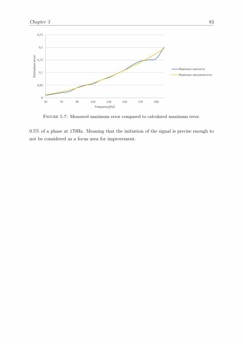
Chapter 5 83

Figure 5.7: Measured maximum error compared to calculated maximum error.

0.5% of a phase at 170Hz. Meaning that the initiation of the signal is precise enough tonot be considered as a focus area for improvement.

Chapter 6

Discussion

The goal of the discussion consists of the three parts presented in the list below.

1. First to discuss if the simulations are representable and how the results from thesesimulations should be used.

2. Secondly to discus whether the physical test bench and the components chosen arewell suited to demonstrate active damping systems or not.

3. Thirdly to discuss if an Arduino is suited for regulating the active damping system.

6.1 Simulations

Simulations are representations of the real world and some simplifications are made.Factors like humidity, temperature, noise from the surroundings are not included in thesimulations. All the factors that affect the simulated test bench are therefor not addressed,only the assumed most important factors. The factors not implemented are considerednot to affect the results in any significant way. The setup of the simulations is the mainfactor that determines how well it represents the physical test bench. The setup in thisthesis is assumed to be fairly good, but improvements are possible with more data fromtesting.

The materials used in the simulations are chosen from the material list provided by theNX software. The material properties of the metals used in the real test bench, however,have not been investigated. This was not done because it is assumed that the potential

84

Chapter 6 85

effect on the results would be neglectable when typical values were used in the simulations.The weight of the parts is the most important property for the metal parts. The partswere control weighed to compare to the simulations and make potential adjustments inthe simulations. No changes were made due to weight difference between measure andsimulated weight.

FEDEM only operates with linear elastic materials. The most important disadvantage ofthe linear representation is that the modeling of the rubber. The rubber has viscoelasticbehavior in real life and the deformation of the rubber in the simulations are linear elastic.The stiffness of the rubber would be affected by the speed of the compression and themagnitude force acting on it. This could be modeled with by using data from testingof the rubber and adding a set dampers to the rubber making a KelvinâĂŞVoigt modelrepresentation of the viscoelastic rubber.

The simulations where the actuators had a flexure represented by one part seemed to givea better representation of the sphere displacement compared to the simulation where theflexure was modelled with eight parts. This can bee seen by comparing figure 3.16 andfigure 4.10. The actuators had an almost linear relationship as described in the data sheet4.10. Further tests should be conducted to verify that the simulated actuators behavein the same way as the physical actuators. The results from the tests should be used toadjust the parameters in the simulations to minimize the deviation.

The eight parts used for representing the flexure of the actuators actuators were modeledwith RBE2 connections and with a spring representing the piezoelectric stack and theflexure was connected. Choosing the stiffness and displacements of the spring used inthe simulations were obtained by adjusting the spring stiffness and the stress free lengthof the spring so that the actuators gave the correct displacement and blocking force.However since the values used in the simulation model are far from the values presentedin the data sheet, we can assume that the simulated model may behave differently fromthe actual actuator.

In the simulations the counter mass is connected to the top of the sphere of the flexurewith a rigid joint. This is not like it is in the physical test bench. In the test bench thecounter mass is placed on top of the spheres and is pushed down with the force comingfrom the tightened spring. The simulated test bench was made this way to eliminatesimulation errors that occurred when other joints were used.

In the simulations the regulating signals are smooth and there is no deviation from the sentsignal to the received signal or noise. In real life applications there will be noise altering

Chapter 6 86

the signals slightly. This will probably increase the requirements for the regulating scriptsince the noise may increase the error of the measurements.

Since the simulated test bench does not act like a vibration absorber, there is a differencein the fundamental dynamic behaviour of the test bench and the simulated test bench.The simulated test bench without the counter weight, spring, washer and bolt had thesame behaviour as the results from Vibration View, after the stiffness of the rubber wasadjusted. The effective stiffness of the rubber can be calculated by rearranging equation2.22 and 2.12.

k = ω2m = 1.6(2π178)2 = 2001335Nm

(6.1)

The error occurred when the parts mentioned above were included in the simulations.Because of this it is assumed that the reason why the complete test bench did not actlike a vibration absorber is due to the modeling of the actuators and how the countermass is modeled to be connected to the actuators. The results from the simulations ofthe components show that the simulations give a good representation of the components’main physical properties. However there were some differences in the results from thesimulations compared to the real life testing when all the components were included inthe MBS. The results from the simulations should therefor be used for describing generalproperties and not to focus on the exact values found.

To find the optimal phase delay from the the measured accelerometer signals to theinitiation of the regulating script, physical tests should be conducted. The optimal phasecan be found in the same way as in the simulations by investigating the effect of delayon the vibrations.

The virtual models used for simulations were adjusted to fit the results from the real liferesults from the shaker. The stiffness and damping of the rubber was adjusted and simu-lating of the piezoelectric stack. This resulted in the simulations being more representableof the physical test bench.

The simulations represented the physical behaviour of the test bench and its componentsrelatively good. The deviations from the simulated dynamic response occurred when thecounter mass, spring bolt and washer were included in the simulations. The error itassumed to arise due to the modeling of the actuators. However the general dynamicbehaviour is assumed to give a representation of the real test bench that can be used to

Chapter 6 87

determine the general properties. Therefore exact values should only be used to give anindication of what the values should be.

6.2 Test bench as demonstrator for active damping

The calculations used for designing the mechanical setup are simplified versions of the realapplications. Therefor deviations between calculated properties and measured propertiesare to be expected. The natural frequency the rubber was dimensioned after was 100Hz,this frequency was calculated to increase to 136Hz when including the structural stiffness.The measured natural frequency of the test bench was however 178Hz. The increase from136Hz to 178Hz may be a result from the viscoelastic properties of the rubber. With alower eigenfrequency of the test bench a working demonstration of the regulating systemwould have less demanding requirements to the scripts and the regulating components.Therefor a real life demonstration could be achieved with less demands for the regulatingsystem.

Achieving a lower natural frequency of the physical test bench is done by using a rubberwith a lower stiffness. Changing the rubber is easy since the test bench is designed with anexchangeable rubber sandwich. Further the test bench can easily change the compressingspring and the counter mass if other physical properties of the test bench is desired.An extra disc can also be mounted between the rubber sandwich and the main mass toincrease the vibrating mass the actuators are designed to reduce. This would also reducethe natural frequency of the test bench as shown by equation 2.65.

The chosen actuators were easily mounted with the screw holes on the protection cover.The design of the main mass made adjusting distance between the center of the mainmass and the actuator possible. This might be practical if the counter mass of the testbench is changed with some other mass with different geometry. The discs made for thetest bench were made with a flat cross section so that there were no unwanted wigglingbetween the plates. The parts were designed with tolerances and clearances so the testbench was easily assembled. The spring was easy to compress using the bolt to regulatethe compression. The compressing of the spring with the bolt has a resolution of 8.4Npr revolution making the load from the spring fairly accurate. It is recommended tocreate a mark on the bolt to make it easier to see the rotation of the bolt and count therevolutions. The test bench as a whole was easy to move, assemble, mount on the shakerand parts were easily changed when desired.

Chapter 6 88

The actuators were designed in a way that made the design of the main mass fairly easyand the actuators are easily regulated by voltage and do not need any external regulation.According to the data sheet and using the theory presented in chapter 2, the actuatorchosen are well suited for being the actuator in a active damping system. To ensure thatthe actuator can operate at the desired frequencies with the full amplitude, testing at thelaboratory should be conducted. These test should also be done with the counter massmounted to see if the actuator behaves as described in the data sheet. Tests to investigatethe phase delay of the regulating signals from the Arduino and the acceleration of themain mass will give needed data for the regulating script. The delay is needed to instructthe Arduino when the initiation of the regulating signal controlling the actuators shouldstart. The delay should also be included in the simulations.

The slew rate of the amplifier can be a restricting factor. This can be investigated byrunning a a frequency sweep test with a constant voltage amplitude. If the stroke of theactuator decreases with the frequency of the signal, the the slew rate probably is notsufficient. The amplifier used in this paper is an old Piezomechanic LE 200/150-1. Datasheet for this amplifier is not available due to its age. One of the more critical drawbackswith this amplifier is that it has only one output channel. The current from the outputchannel of the amplifier has to provide current demanded by all three actuators. A wayto ensure that the amplifier is not a restricting factor is to acquire an amplifier with thedesired properties. Thorlabs sells amplifiers designed to control piezoelectric actuators,some with three output channels and high current output. The ”BPC303 - 3-Channel150 V Benchtop Piezo Controller with USB” sold by Thorlabs can provide a 212Hz signalwith 75V peak to peak amplitude[30] with sufficient current for the actuators presentedin this paper from three channels. Therefore this amplifier is recommended by the authorfor the described application.

The simulations show promising result for how well the test bench can reduce the vibra-tions. The simulations showed a vibration reduction of over 90%. This implies that theconcept used for damping the vibrations can give very good results. This vibration reduc-tion is achieved while the peak-to-peak amplitude of the stack displacement is 26.5 µm.The maximum displacement of the stack regulation is 50µm as mentioned in section 4.4.2.The maximum displacement of the stack is roughly double of the displacement used in thesimulations. This implies that the maximum acceleration of the virtual shaker causingthe vibrations of the main mass can be doubled before the actuators are the restrictingfactor at 140Hz. This is an acceleration of about 10m

s2 or 1g. The acceleration will varywith the frequency as can be seen from equation 2.15 and figure 2.3. The maximum

Chapter 6 89

acceleration the shaker can provide when the actuators as the restricting factor is shownas a function of frequency in figure 6.1. This was calculated by using equation 2.15 andthe restriction of 1g as maximum acceleration at 140Hz

Figure 6.1: Maximum acceleration exerted by the shaker which the actuators candampen optimally

By increasing the displacement of the actuators an increase in the vibrations of the mainmass was shown in the simulation output. The maximum vibration damping at 140Hzwas reduced as a result of a reduced displacement of the virtually regulated stack. At thesame time the span of the fraction of the phase where damping was achieved increased.This means that there is a trade of with damping effect and span width where damping isachieved. This should be further investigated to find the best suited stack displacementwhen the precision of the script is known since this phase span determines the precisiondemand of the regulating script.

The results from the simulations show the span of where the actuation of the actuatorsreduce the vibrations to be about 0.3 of the oscillation period. This fraction can be higherif a lower stack displacement is used resulting in a reduced maximum damping effect.

In general the test bench should be able to demonstrate active vibration damping in therange of 100Hz to 200Hz when the accelerations are kept under the restriction given infigure 6.1. The time period fraction of 0.3 of a period is fairly small and decreasing with

Chapter 6 90

an increasing frequency. This should however be possible to regulate with a precise andaccurate regulation system.

6.3 Arduino as control mechanism

The voltage output for 1g acceleration of the ADXL335 accelerometer varies with thefrequency. This is in this paper handled by using an equation to adjust the signal tonormalize it with respect to the frequency. An ideal accelerometer should not give differentvoltage outputs when the frequency is within the bandwidth of the accelerometer.

By changing the ADXL335 with an accelerometer with an output independent of fre-quency, less calculations have to be run in the code, making the code faster. Further,equation 4.3 is a source to error that can reduce the precision of the regulating algorithm.The elimination of the frequency dependency of the voltage output to the Arduino mayalso be obtained by changing the circuit of the Arduino setup.

The noise in the circuit is fairly low as shown in tables 4.1 and 4.2. For the ADXL335accelerometer this will result on an maximum reading error of 0.04g due to the noise inthe circuit. This will most likely not result in any implications that will noticeably reducethe damping properties of the active damping system.

The noise will also affect the data used for estimating the frequency. The error that ispresented in figure 5.7 and explained by equation 5.2 can be reduced and even eliminatedby using a linear regression to estimate the exact time value when the signal from theaccelerometer crosses the average. If a linear regression is used for this, the noise will be anissue and might result in error in the frequency estimation. The error caused by the noisehas little effect on the precision of the initiation of the regulating signal. One possibleway to reduce the implications of an error in the estimation is to reduce the numberof samples used to calculate the frequency. Reducing the number of measurements tohalf allows the error to be twice as large with the same phase error after the signal hasoscillated the number of periods equal to the sample size.

The Arduino Due has a clock speed at 84MHz, which means the CPU is 5.25 times fasterthan the Arduino UNO. The speed of the CPU is sufficient to do simple calculations withsub microsecond speed. By avoiding float numbers in complex formulas the high codespeed result in a sufficient code speed for calculations. Data from the analog pins canbe read or written within 2 µs. The main issue for using the Arduino to regulate the

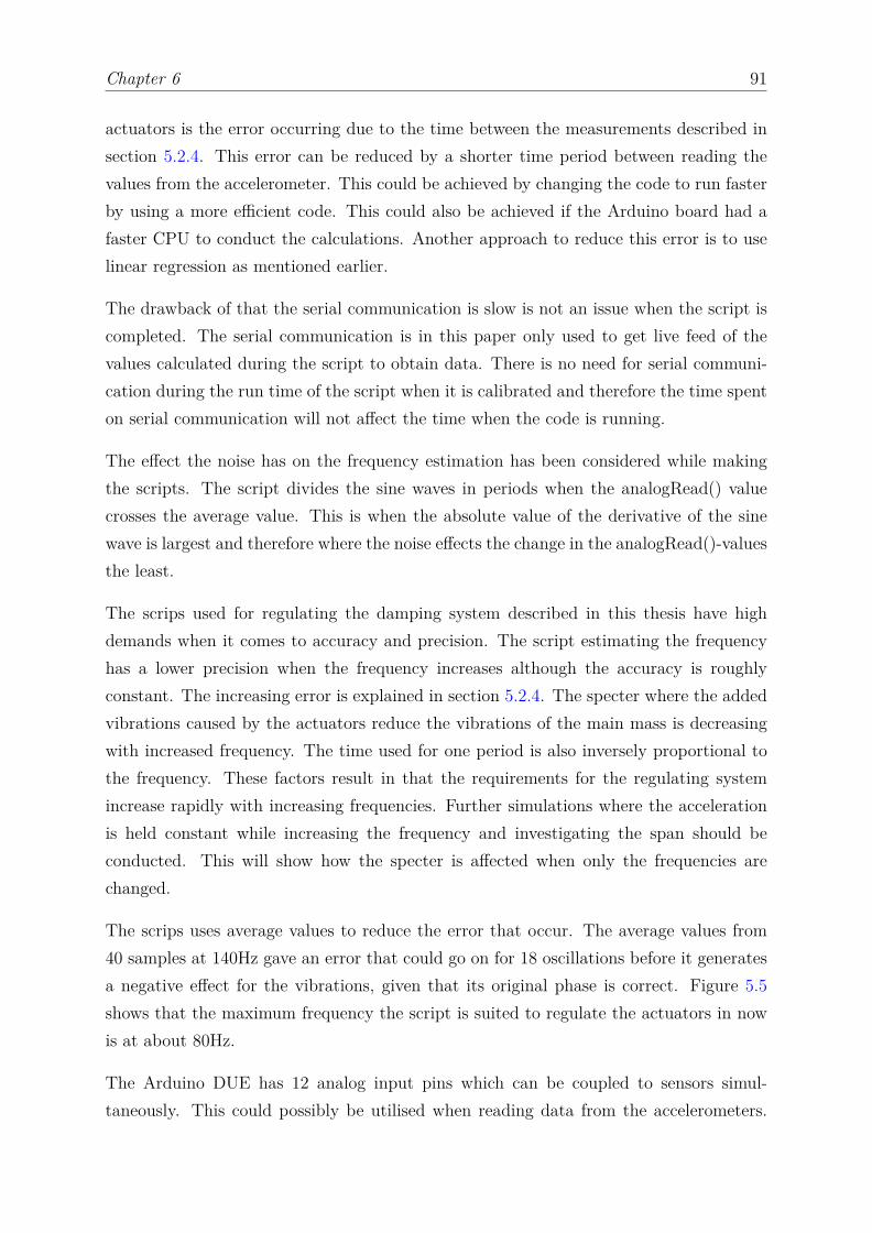
Chapter 6 91

actuators is the error occurring due to the time between the measurements described insection 5.2.4. This error can be reduced by a shorter time period between reading thevalues from the accelerometer. This could be achieved by changing the code to run fasterby using a more efficient code. This could also be achieved if the Arduino board had afaster CPU to conduct the calculations. Another approach to reduce this error is to uselinear regression as mentioned earlier.

The drawback of that the serial communication is slow is not an issue when the script iscompleted. The serial communication is in this paper only used to get live feed of thevalues calculated during the script to obtain data. There is no need for serial communi-cation during the run time of the script when it is calibrated and therefore the time spenton serial communication will not affect the time when the code is running.

The effect the noise has on the frequency estimation has been considered while makingthe scripts. The script divides the sine waves in periods when the analogRead() valuecrosses the average value. This is when the absolute value of the derivative of the sinewave is largest and therefore where the noise effects the change in the analogRead()-valuesthe least.

The scrips used for regulating the damping system described in this thesis have highdemands when it comes to accuracy and precision. The script estimating the frequencyhas a lower precision when the frequency increases although the accuracy is roughlyconstant. The increasing error is explained in section 5.2.4. The specter where the addedvibrations caused by the actuators reduce the vibrations of the main mass is decreasingwith increased frequency. The time used for one period is also inversely proportional tothe frequency. These factors result in that the requirements for the regulating systemincrease rapidly with increasing frequencies. Further simulations where the accelerationis held constant while increasing the frequency and investigating the span should beconducted. This will show how the specter is affected when only the frequencies arechanged.

The scrips uses average values to reduce the error that occur. The average values from40 samples at 140Hz gave an error that could go on for 18 oscillations before it generatesa negative effect for the vibrations, given that its original phase is correct. Figure 5.5shows that the maximum frequency the script is suited to regulate the actuators in nowis at about 80Hz.

The Arduino DUE has 12 analog input pins which can be coupled to sensors simul-taneously. This could possibly be utilised when reading data from the accelerometers.

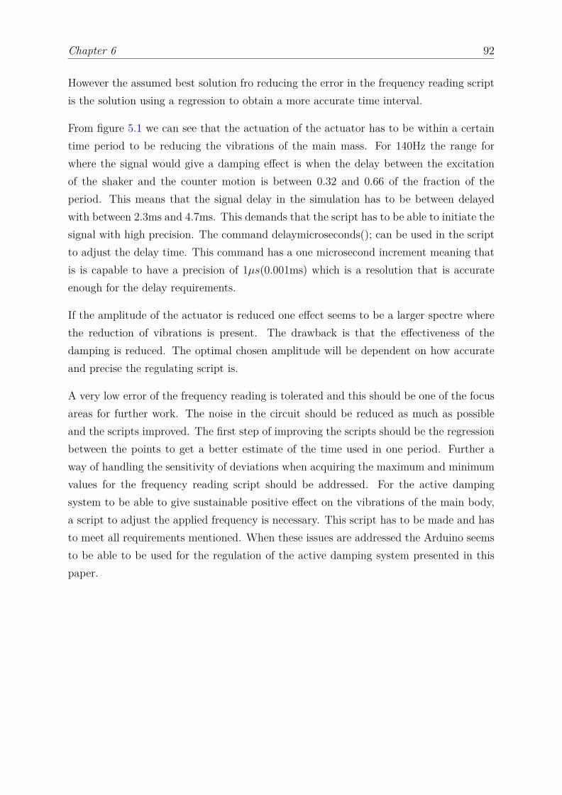
Chapter 6 92

However the assumed best solution fro reducing the error in the frequency reading scriptis the solution using a regression to obtain a more accurate time interval.

From figure 5.1 we can see that the actuation of the actuator has to be within a certaintime period to be reducing the vibrations of the main mass. For 140Hz the range forwhere the signal would give a damping effect is when the delay between the excitationof the shaker and the counter motion is between 0.32 and 0.66 of the fraction of theperiod. This means that the signal delay in the simulation has to be between delayedwith between 2.3ms and 4.7ms. This demands that the script has to be able to initiate thesignal with high precision. The command delaymicroseconds(); can be used in the scriptto adjust the delay time. This command has a one microsecond increment meaning thatis is capable to have a precision of 1µs(0.001ms) which is a resolution that is accurateenough for the delay requirements.

If the amplitude of the actuator is reduced one effect seems to be a larger spectre wherethe reduction of vibrations is present. The drawback is that the effectiveness of thedamping is reduced. The optimal chosen amplitude will be dependent on how accurateand precise the regulating script is.

A very low error of the frequency reading is tolerated and this should be one of the focusareas for further work. The noise in the circuit should be reduced as much as possibleand the scripts improved. The first step of improving the scripts should be the regressionbetween the points to get a better estimate of the time used in one period. Further away of handling the sensitivity of deviations when acquiring the maximum and minimumvalues for the frequency reading script should be addressed. For the active dampingsystem to be able to give sustainable positive effect on the vibrations of the main body,a script to adjust the applied frequency is necessary. This script has to be made and hasto meet all requirements mentioned. When these issues are addressed the Arduino seemsto be able to be used for the regulation of the active damping system presented in thispaper.

Chapter 7

Conclusion and Further Work

The test bench was modeled and produced to fit the chosen actuators. The test benchwas easily mounted on the shaker provided and the regulating system using an ArduinoDue was easily mounted. Simulations for analysing the dynamics of the test bench wereconducted and scripts on the Arduino were investigated. The speed and precision of theresults form the scripts were compared to the demands obtained form the simulations.

The general behaviour of the components in the simulation model behave as desired wheninvestigated as independent components. However when they are combined in the MBSwith all parts included the general dynamics of the virtual test bench was not as themeasured dynamics of the real test bench.

The difference between the virtual and real the bench is assumed to be a result for themodeling of the piezoelectric actuators. The results from the simulations were used todescribe the general behaviour. The maximum reduction of the vibrations achieved inthe simulations was about 90% compared to when the actuators were inactive. The phaseof the signal regulating the actuators affect the vibration reduction. The phase of theactuators must be regulated wit sub millisecond precision.

The precision of the script estimating the frequencies is not good enough as it is presentedin this paper. The demands for the script increase while the precision decreases with anincrease of frequency. The script presented is precise enough to regulate be used for regu-lating a system of about 80Hz and below when assuming perfect phase initiation. Furtherwork on the scripts measuring the frequency and the initiation of the signal is imperativefor the active damping system to preform. The relationship between the measured accel-eration and the applied displacement which gives the most effective vibration reduction is

93

Chapter 94

not obtained in this thesis. This should however be obtained either by simulations or byresults form physical testing before the script regulating the active damping is suitable.

An amplifier better suited for regulating the actuators should be used for regulatingthe actuators. Furthermore noise from the accelerometer should be reduced or an otheraccelerometer should be used. The simulations of the actuator should be improved for theto make the simulations of the test bench more representable of the physical test bench.

Appendix A

Appendix

int Voltage = 0;int maxVoltage=0;int minVoltage=4094;int spanVoltage=0;int noice=0;int Current=0;int SampleSize=0;int Average=0;int initiate=0;int state=0;int mwp=0;int grit=0;int trig=0;int pwm=0;int Print=0;int amplitude=0;int enableActuator=0;int startAcceleration=0;int count=0;unsigned long Tid=0;unsigned long Tid1=0.00;unsigned long tidSig=0;unsigned long TidPhase=0;float sample=0.00;

95

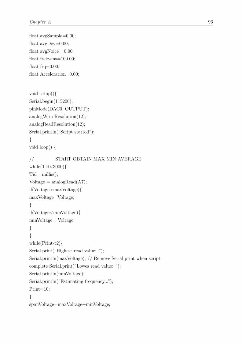
Chapter A 96

float avgSample=0.00;float avgDev=0.00;float avgNoice =0.00;float frekvens=100.00;float frq=0.00;float Acceleration=0.00;

void setup(){Serial.begin(115200);pinMode(DAC0, OUTPUT);analogWriteResolution(12);analogReadResolution(12);Serial.println(”Script started”);}void loop() {

//————–START OBTAIN MAX MIN AVERAGE————————while(Tid<3000){Tid= millis();Voltage = analogRead(A7);if(Voltage>maxVoltage){maxVoltage=Voltage;}if(Voltage<minVoltage){minVoltage =Voltage;}}while(Print<2){Serial.print(”Highest read value: ”);Serial.println(maxVoltage); // Remove Serial.print when scriptcomplete Serial.print(”Lowes read value: ”);Serial.println(minVoltage);Serial.println(”Estimating frequency...”);Print=10;}spanVoltage=maxVoltage+minVoltage;

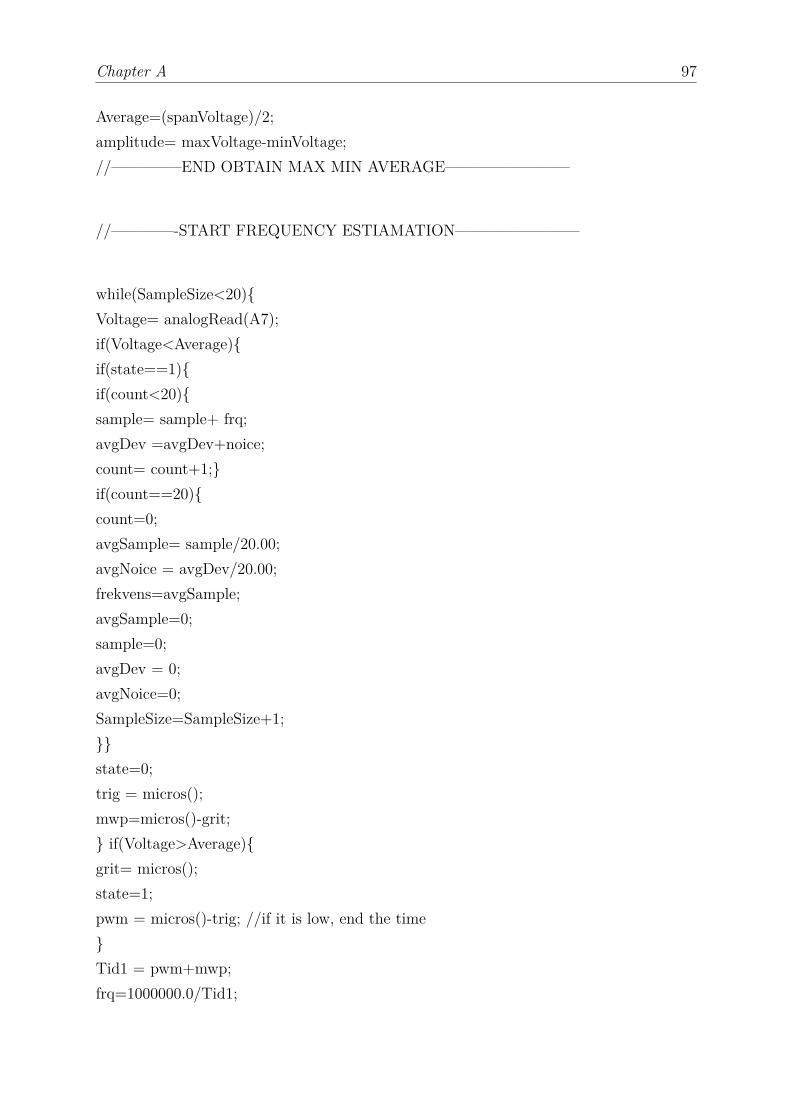
Chapter A 97

Average=(spanVoltage)/2;amplitude= maxVoltage-minVoltage;//————–END OBTAIN MAX MIN AVERAGE————————

//————-START FREQUENCY ESTIAMATION————————

while(SampleSize<20){Voltage= analogRead(A7);if(Voltage<Average){if(state==1){if(count<20){sample= sample+ frq;avgDev =avgDev+noice;count= count+1;}if(count==20){count=0;avgSample= sample/20.00;avgNoice = avgDev/20.00;frekvens=avgSample;avgSample=0;sample=0;avgDev = 0;avgNoice=0;SampleSize=SampleSize+1;}}state=0;trig = micros();mwp=micros()-grit;} if(Voltage>Average){grit= micros();state=1;pwm = micros()-trig; //if it is low, end the time}Tid1 = pwm+mwp;frq=1000000.0/Tid1;

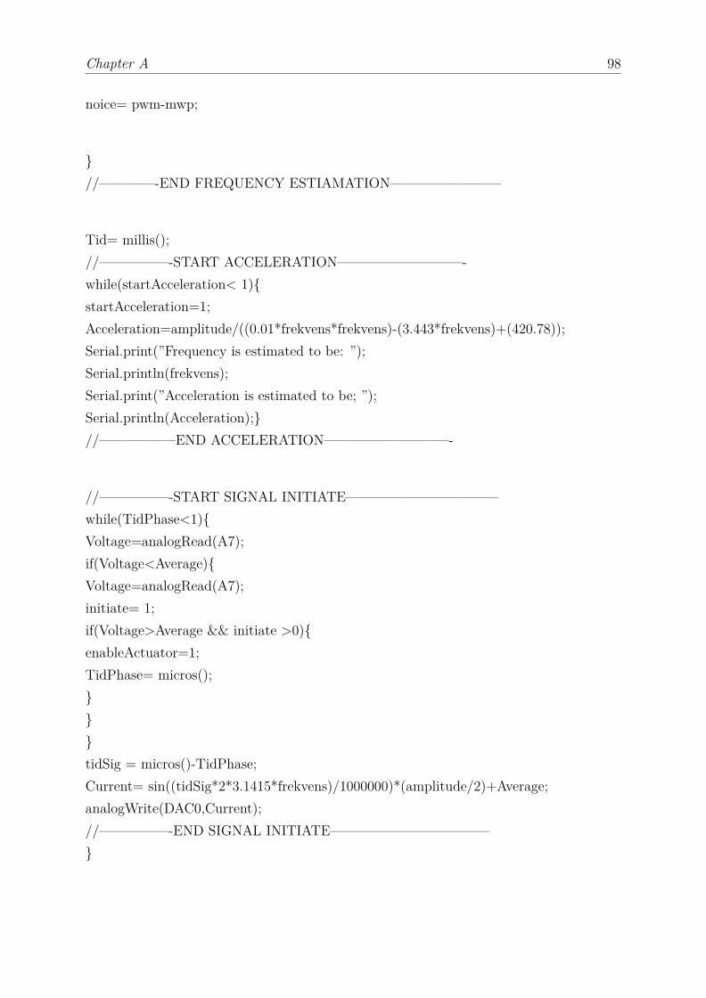
Chapter A 98

noice= pwm-mwp;

}//————-END FREQUENCY ESTIAMATION————————

Tid= millis();//—————-START ACCELERATION—————————-while(startAcceleration< 1){startAcceleration=1;Acceleration=amplitude/((0.01*frekvens*frekvens)-(3.443*frekvens)+(420.78));Serial.print(”Frequency is estimated to be: ”);Serial.println(frekvens);Serial.print(”Acceleration is estimated to be; ”);Serial.println(Acceleration);}//—————–END ACCELERATION—————————-

//—————-START SIGNAL INITIATE———————————while(TidPhase<1){Voltage=analogRead(A7);if(Voltage<Average){Voltage=analogRead(A7);initiate= 1;if(Voltage>Average && initiate >0){enableActuator=1;TidPhase= micros();}}}tidSig = micros()-TidPhase;Current= sin((tidSig*2*3.1415*frekvens)/1000000)*(amplitude/2)+Average;analogWrite(DAC0,Current);//—————-END SIGNAL INITIATE———————————–}

Bibliography

[1] Birk Brockmann Christian Brecher, Stephan Baumler. Avoiding chatter by meansof active damping systems for machine tools. Journal of Machine Engineering, 13(3), 2013.

[2] Thorlabs piezoelectric theory. https://www.thorlabs.de/NewGroupPage9.cfm?

ObjectGroup_ID=5030, . Accessed: 2017-04-16.

[3] Thorlabs pk2fvf1 - amplified piezoelectric actuator with flexure mount. https://

www.thorlabs.de/thorproduct.cfm?partnumber=PK2FVF1. Accessed: 2017-02-05.

[4] N Lhermet A. Harms, B Denkena. Tool adaptor for active vibration controll inturning operations. 9th International Concerance on New Actuators, Germany, 2004.

[5] M. Horodinca A. Premount A.Ganguli, A. Deraemaeker. Active damping of chatterin machine tools-demonstration with a ”hardware in the loop” simulator. Journal ofSystems and Control Engineering, 219, 2005.

[6] H. Frahm. Device for damping vibrations of bodies., April 18 1911. URL http:

//www.google.no/patents/US989958. US Patent 989,958.

[7] C. Collette S.ChesnÃĺ. A simple hybridization of active and passive mass dampers.ISMA conferance, 2016.

[8] A. von Flotow N.w. Hagood. Damping of structural vibrations with piezoelectricmaterials and passive electrical networks. Journal of Sound and Vibration, 1991.

[9] Valder Steffen Jr Felipe Antonio C. Viana. Multimodal vibration damping throughpiezoelectric patches and optimal resonant shunt circuits. Journal of the BrazilianSociety of Mechanical Sciences and Engineering, 28, 2006.

[10] Iwao Yamaji Atsushi Matsubara, Minetaka Maeda. Vibration suppression of boringbar by piezoelctric actuators and lr circuit. Elesevier, 2014.

99

https://www.thorlabs.de/NewGroupPage9.cfm?ObjectGroup_ID=5030

https://www.thorlabs.de/NewGroupPage9.cfm?ObjectGroup_ID=5030

https://www.thorlabs.de/thorproduct.cfm?partnumber=PK2FVF1

https://www.thorlabs.de/thorproduct.cfm?partnumber=PK2FVF1

http://www.google.no/patents/US989958

http://www.google.no/patents/US989958

Bibliography 100

[11] L. Walter J. Millitzer J. Rohlfing, T. May. Self-tuning velocity feedback control for atime varying structure using a voltage driven electromagnetic inertial mass actuator.ISMA, 2016.

[12] Alessandro D’Ausilio. Arduino: A low-cost multipurpose lab equipment. Springer,2011.

[13] Arduino UNO overview, technical specifications and documentation. https://www.

arduino.cc/en/Main/ArduinoBoardUno, . Accessed: 2016-04-13.

[14] Bill Drury Austin Hughes. Electric Motors and Drives (Fourth Edition). Interna-tional series of monographs on physics. Newnes, 2013. ISBN 978-0-08-098332-5.

[15] Arduino comparing comparing boards. https://www.arduino.cc/en/Products/

Compare, . Accessed: 2016-04-13.

[16] Arduino memory learning memory. https://www.arduino.cc/en/Tutorial/

Memory, . Accessed: 2016-04-13.

[17] Arduino sketch learning sketch. https://www.arduino.cc/en/tutorial/sketch, .Accessed: 2016-04-13.

[18] Arduino Library library. https://www.arduino.cc/en/Reference/Libraries, .Accessed: 2016-04-13.

[19] R. Hooke. Lectures de Potentia Restitutiva, Or of Spring Explaining the Power ofSpringing Bodies. [Cutlerian lecture. John Martyn, 1678. URL https://books.

google.co.uk/books?id=LAtPAAAAcAAJ.

[20] R.C.Hibbeler. Mechanics of Materials, Eighth edition in SI units. Pearson, 2011.ISBN 978-981-06-8504-6.

[21] Gene Mosca Paul A. Tipler. Physics for Scientists and Engineers, sixth edition.Freeman, 2008. ISBN 978-0-7167-8964-2.

[22] Fridtjov Irgens. Fastetsære, 7th edition. Tapir Akademisk Forlag, 2006. ISBN 82-519-2137-6.

[23] David G. Rethwisch William D. Callister. Materials Science and Engineering, 8thedition. John Wiley and Sons, 2011. ISBN 978-0-470-50586-1.

[24] Marie Dillon Dahleh William T. Thomson. Theory of vibration with applications.Prentice Hall, 1998. ISBN 0-13-651068-X.

https://www.arduino.cc/en/Main/ArduinoBoardUno

https://www.arduino.cc/en/Main/ArduinoBoardUno

https://www.arduino.cc/en/Products/Compare

https://www.arduino.cc/en/Products/Compare

https://www.arduino.cc/en/Tutorial/Memory

https://www.arduino.cc/en/Tutorial/Memory

https://www.arduino.cc/en/tutorial/sketch

https://www.arduino.cc/en/Reference/Libraries

https://books.google.co.uk/books?id=LAtPAAAAcAAJ

https://books.google.co.uk/books?id=LAtPAAAAcAAJ

Bibliography 101

[25] L. G. Kraige J.L. Meriam. Dynamics,SI edition, seventh edition. Engineering Me-chanics. John Wiley and Sons, 2013. ISBN 978-1-118-08345-1.

[26] Erwin Kreysig. Advanced Engineeting Mathematics, tenth edition. John Wiley andSons, INC, 2011. ISBN 978-47064613-7.

[27] Physik Instrumente ciezoelectric tutorial. http://www.piezo.ws/piezoelectric_

actuator_tutorial/Piezo_Design_part3.php. Accessed: 2017-02-05.

[28] Piezomechnaic products brochures pdf. http://www.piezomechanik.com/

products/. Accessed: 2017-04-16.

[29] Gunnar Harkegard. Dimensjonering av maskindeler, 2nd edition. Tapir AkademiskForlag, 2012. ISBN 978-82-519-1970-8.

[30] BPC303 - 3-Channel 150 V Benchtop Piezo Controller with USB overview, techni-cal specifications and documentation. https://www.thorlabs.de/newgrouppage9.

cfm?objectgroup_id=1912, . Accessed: 2017-04-13.

http://www.piezo.ws/piezoelectric_actuator_tutorial/Piezo_Design_part3.php

http://www.piezo.ws/piezoelectric_actuator_tutorial/Piezo_Design_part3.php

http://www.piezomechanik.com/products/

http://www.piezomechanik.com/products/

https://www.thorlabs.de/newgrouppage9.cfm?objectgroup_id=1912

https://www.thorlabs.de/newgrouppage9.cfm?objectgroup_id=1912

Active and passive damping systems for vibration control ......Active and passive damping systems...

Documents

Transcript of Active and passive damping systems for vibration control ......Active and passive damping systems...