ACTEX STAM EXAM MANUAL - TABLE OF CONTENTSsheldon/ACT451-2019/Sections-1-6.pdf · Actex Learning...
94
Actex Learning SOA Exam STAM - Short-Term Actuarial Mathematics ACTEX STAM EXAM MANUAL - TABLE OF CONTENTS INTRODUCTORY COMMENTS NOTES AND PROBLEM SETS SECTION 1 - Preliminary Review - Probability 1 PROBLEM SET 1 9 SECTION 2 - Preliminary Review - Random Variables I 19 PROBLEM SET 2 29 SECTION 3 - Preliminary Review - Random Variables II 33 PROBLEM SET 3 43 SECTION 4 - Preliminary Review - Random Variables III 51 PROBLEM SET 4 59 SECTION 5 - Parametric Distributions and Transformations 65 PROBLEM SET 5 73 SECTION 6 - Distribution Tail Behavior 81 PROBLEM SET 6 85 SECTION 7 - Mixture of Two Distributions 87 PROBLEM SET 7 93 SECTION 8 - Mixture of Distributions 101 8 PROBLEM SET 8 107 SECTION 9 - Continuous Mixtures 115 PROBLEM SET 9 121 SECTION 10 - Frequency Models 129 PROBLEM SET 10 137 SECTION 11 - Policy Limits 155 PROBLEM SET 11 159 SECTION 12 - Policy Deductible (1), The Cost Per Loss 161 PROBLEM SET 12 167 SECTION 13 - Policy Deductible (2), The Cost Per Loss 179 PROBLEM SET 13 185 SECTION 14 - Deductibles Applied to the Uniform, Exponential and Pareto Distributions 197 PROBLEM SET 14 205
Transcript of ACTEX STAM EXAM MANUAL - TABLE OF CONTENTSsheldon/ACT451-2019/Sections-1-6.pdf · Actex Learning...
Actex Learning SOA Exam STAM - Short-Term Actuarial Mathematics
ACTEX STAM EXAM MANUAL - TABLE OF CONTENTS
INTRODUCTORY COMMENTS
NOTES AND PROBLEM SETS
SECTION 1 - Preliminary Review - Probability 1PROBLEM SET 1 9
SECTION 2 - Preliminary Review - Random Variables I 19PROBLEM SET 2 29
SECTION 3 - Preliminary Review - Random Variables II 33PROBLEM SET 3 43
SECTION 4 - Preliminary Review - Random Variables III 51PROBLEM SET 4 59
SECTION 5 - Parametric Distributions and Transformations 65PROBLEM SET 5 73
SECTION 6 - Distribution Tail Behavior 81PROBLEM SET 6 85
SECTION 7 - Mixture of Two Distributions 87PROBLEM SET 7 93
SECTION 8 - Mixture of Distributions 1018PROBLEM SET 8 107
SECTION 9 - Continuous Mixtures 115PROBLEM SET 9 121
SECTION 10 - Frequency Models 129PROBLEM SET 10 137
SECTION 11 - Policy Limits 155PROBLEM SET 11 159
SECTION 12 - Policy Deductible (1), The Cost Per Loss 161PROBLEM SET 12 167
SECTION 13 - Policy Deductible (2), The Cost Per Loss 179PROBLEM SET 13 185
SECTION 14 - Deductibles Applied to the Uniform, Exponential and Pareto Distributions 197PROBLEM SET 14 205

Actex Learning SOA Exam STAM - Short-Term Actuarial Mathematics
SECTION 15 - Combined Limit and Deductible 209PROBLEM SET 15 215
SECTION 16 - Additional Policy Adjustments 231PROBLEM SET 16 235
SECTION 17 - Models for the Aggregate Loss, Compound Distributions (1) 243PROBLEM SET 17 247
SECTION 18 - Compound Distributions (2) 271PROBLEM SET 18 277
SECTION 19 - More Properties of the Aggregate Loss Random Variable 291PROBLEM SET 19 295
SECTION 20 - Stop Loss Insurance 313PROBLEM SET 20 321
SECTION 21 - Risk Measures 331PROBLEM SET 21 335
SECTION 22 - Data and Estimation Review 339
SECTION 23 - Maximum Likelihood Estimation Based on Complete Data 343PROBLEM SET 23 347
SECTION 24 - Maximum Likelihood Estimation Based on Incomplete Data 355PROBLEM SET 24 363
SECTION 25 - Maximum Likelihood Estimation for the Exponential Distribution 369PROBLEM SET 25 375
SECTION 26 - MLE Applied to Pareto and Weibull Distributions 383PROBLEM SET 26 393
SECTION 27 - MLE Applied to STAM Exam Table Distributions 403PROBLEM SET 27 413
SECTION 28 - Review of Mathematical Statistics 423PROBLEM SET 28 431
SECTION 29 - Properties of Maximum Likelihood Estimators 437PROBLEM SET 29 441
SECTION 30 - Hypothesis Tests For Fitted Models 451PROBLEM SET 30 463
SECTION 31 - Graphical Methods for Evaluating Fitted Models 485PROBLEM SET 30 489
Actex Learning SOA Exam STAM - Short-Term Actuarial Mathematics
SECTION 32 - Limited Fluctuation Credibility 495PROBLEM SET 32 509
SECTION 33 - Bayesian Estimation, Discrete Prior 527PROBLEM SET 33 537
SECTION 34 - Bayesian Credibility, Discrete Prior 553PROBLEM SET 34 563
SECTION 35 - Bayesian Credibility, Continuous Prior 593PROBLEM SET 35 601
SECTION 36 - Bayesian Credibility Applied to Distributions in STAM Exam Table 625PROBLEM SET 36 635
SECTION 37 - Buhlmann Bayesian 655PROBLEM SET 37 665
SECTION 38 - Empirical Bayes Credibility 713PROBLEM SET 38 721
SECTION 39 - Major Medical and Dental Coverage 749
SECTION 40 - Property and Casualty Coverages 751
SECTION 41 - Loss Reserving 755PROBLEM SET 41 765
SECTION 42 - Ratemaking 779PROBLEM SET 42 787
SECTION 43 - Additional Casualty Insurance Topics 793PROBLEM SET 43 797
PRACTICE EXAMS
PRACTICE EXAM 1 801
PRACTICE EXAM 2 819
PRACTICE EXAM 3 835
PRACTICE EXAM 4 853
PRACTICE EXAM 5 871

Actex Learning SOA Exam STAM - Short-Term Actuarial Mathematics

Actex Learning SOA STAM Exam - Short Term Actuarial Mathematics
INTRODUCTORY COMMENTS
This study guide is designed to help in the preparation for the Society of Actuaries STAM Exam.
The first part of this manual consists of a summary of notes, illustrative examples and problem sets withdetailed solutions. The second part consists of 5 practice exams.
The practice exams all have 35 questions. The level of difficulty of the practice exams has been designedto be similar to that of the past 3.5-hour exams. Some of the questions in the problem sets are taken fromthe relevant topics on SOA exams that have been released prior to 2009 but the practice exam questionsare not from old SOA exams.
I have attempted to be thorough in the coverage of the topics upon which the exam is based, andconsistent with the notation and content of the official references. I have been, perhaps, more thoroughthan necessary on a couple of topics, such as maximum likelihood estimation and Bayesian credibility.
Because of the time constraint on the exam, a crucial aspect of exam taking is the ability to work quickly.I believe that working through many problems and examples is a good way to build up the speed at whichyou work. It can also be worthwhile to work through problems that have been done before, as this helpsto reinforce familiarity, understanding and confidence. Working many problems will also help in beingable to more quickly identify topic and question types. I have attempted, wherever possible, to emphasizeshortcuts and efficient and systematic ways of setting up solutions. There are also occasional commentson interpretation of the language used in some exam questions. While the focus of the study guide is onexam preparation, from time to time there will be comments on underlying theory in places that I feelthose comments may provide useful insight into a topic.
The notes and examples are divided into 42 sections of varying lengths, with some suggested time framesfor covering the material. There are almost 200 examples in the notes and over 900 exercises in theproblem sets, all with detailed solutions. The 5 practice exams have 35 questions each, also with detailedsolutions. Some of the examples and exercises are taken from previous SOA exams. Some of the in theproblem sets that have come from previous SOA exams. Some of the problem set exercises are more indepth than actual exam questions, but the practice exam questions have been created in an attempt toreplicate the level of depth and difficulty of actual exam questions. In total there are almost 1300examples/problems/sample exam questions with detailed solutions. ACTEX gratefully acknowledges theSOA for allowing the use of their exam problems in this study guide.
I suggest that you work through the study guide by studying a section of notes and then attempting theexercises in the problem set that follows that section. The order of the sections of notes is the order that Irecommend in covering the material, although the material on pricing and reserving in Sections 39 to 42is independent of the other material on the exam. The order of topics in this manual is not the same as theorder presented on the exam syllabus.
It has been my intention to make this study guide self-contained and comprehensive for the STAM Examtopics, however there are some exam topics for which the study notes are essentially summaries ofconcepts. For that material, I have attempted to summarize concepts as well, but it is best to refer tooriginal reference material on all topics.
While the ability to derive formulas used on the exam is usually not the focus of an exam question, it isuseful in enhancing the understanding of the material and may be helpful in memorizing formulas. Theremay be an occasional reference in the review notes to a derivation, but you are encouraged to review theofficial reference material for more detail on formula derivations.

Actex Learning SOA STAM Exam - Short Term Actuarial Mathematics
In order for the review notes in this study guide to be most effective, you should have some backgroundat the junior or senior college level in probability and statistics. It will be assumed that you are reasonablyfamiliar with differential and integral calculus. The prerequisite concepts to modeling and modelestimation are reviewed in this study guide. The study guide begins with a detailed review of probabilitydistribution concepts such as distribution function, hazard rate, expectation and variance.
Of the various calculators that are allowed for use on the exam, I am most familiar with theBA II PLUS. It has several easily accessible memories. The TI-30X IIS has the advantage of a multi-line display. Both have the functionality needed for the exam.
There is a set of tables that has been provided with the exam in past sittings. These tables consist of somedetailed description of a number of probability distributions along with tables for the standard normal andchi-squared distributions. The tables can be downloaded from the SOA website www.soa.org .
If you have any questions, comments, criticisms or compliments regarding this study guide, pleasecontact the publisher ACTEX, or you may contact me directly at the address below. I apologize inadvance for any errors, typographical or otherwise, that you might find, and it would be greatlyappreciated if you would bring them to my attention. ACTEX will be maintaining a website for errata thatcan be accessed from www.actexmadriver.com .
It is my sincere hope that you find this study guide helpful and useful in your preparation for the exam. Iwish you the best of luck on the exam.
Samuel A. Broverman Department of Statistical Sciences www.sambroverman.comUniversity of Toronto E-mail: [email protected] or [email protected]
NOTES
AND
PROBLEM SETS

SECTION 1 - PRELIMINARY REVIEW - PROBABILITY STAM-1
Actex Learning SOA Exam STAM - Short-Term Actuarial Mathematics
SECTION 1 - PRELIMINARY REVIEW - PROBABILITYBasic Probability, Conditional Probability and Independence
A significant part of the STAM Exam involves probability and statistical methods applied to various aspects ofloss modeling and model estimation. A good background in probability and statistics is necessary to fullyunderstand models and the modeling that is done. In this section of the study guide, we will review fundamentalprobability rules.
1.1 Basic Probability Concepts
Sample point and probability spaceA sample point is the simple outcome of a random experiment. The probability space (also called sample space) isthe collection of all possible sample points related to a specified experiment. When the experiment is performed,one of the sample points will be the outcome. An experiment could be observing the loss that occurs on anautomobile insurance policy during the course of one year, or observing the number of claims arriving at aninsurance office in one week. The probability space is the "full set" of possible outcomes of the experiment. In thecase of the automobile insurance policy, it would be the range of possible loss amounts that could occur duringthe year, and in the case of the insurance office weekly number of claims, the probability space would be the setof integers .Ö!ß "ß #ß ÞÞÞ×
EventAny collection of sample points, or any subset of the probability space is referred to as an event. We say "event Ehas occurred" if the experimental outcome was one of the sample points in .E
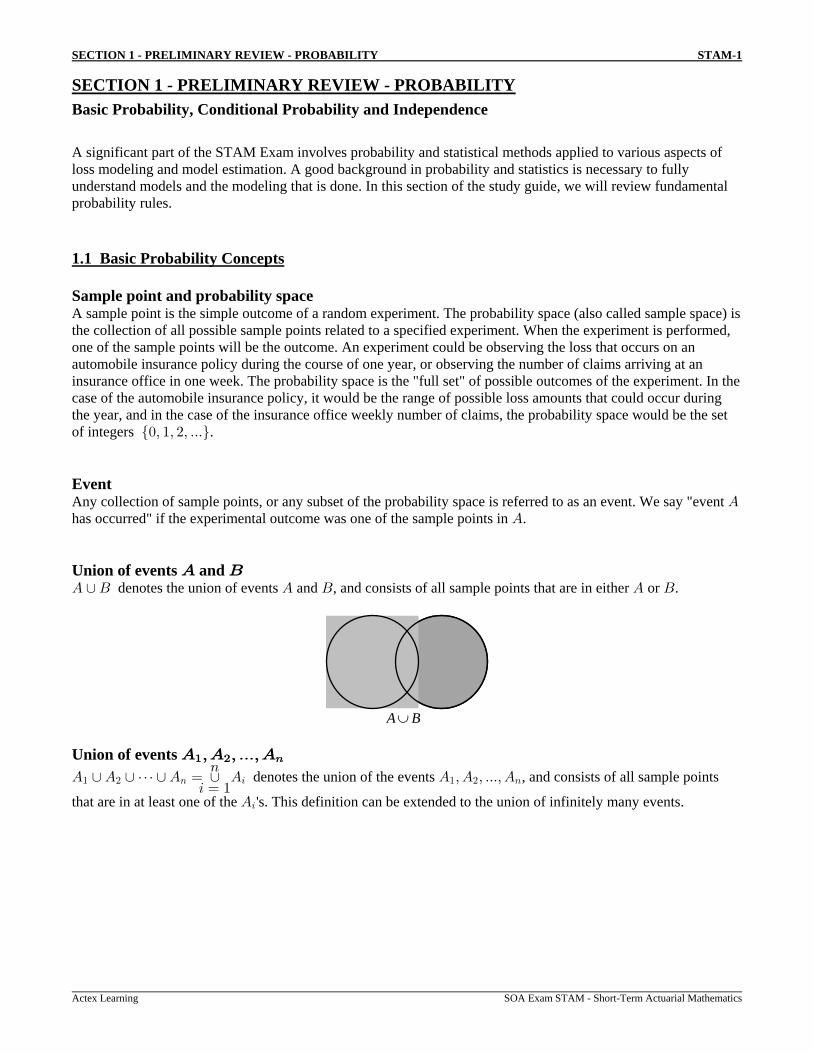
Union of events and E FE ∪ F E F E F denotes the union of events and , and consists of all sample points that are in either or .
A B Union of events E ßE ß ÞÞÞßE" # 8
E ∪ E ∪â∪E œ ∪ E E ßE ß ÞÞÞß E3 œ "
8" # 8 3 " # 8 denotes the union of the events , and consists of all sample points
that are in at least one of the 's. This definition can be extended to the union of infinitely many events.E3
STAM-2 SECTION 1 - PRELIMINARY REVIEW - PROBABLITY
Actex Learning SOA Exam STAM - Short-Term Actuarial Mathematics
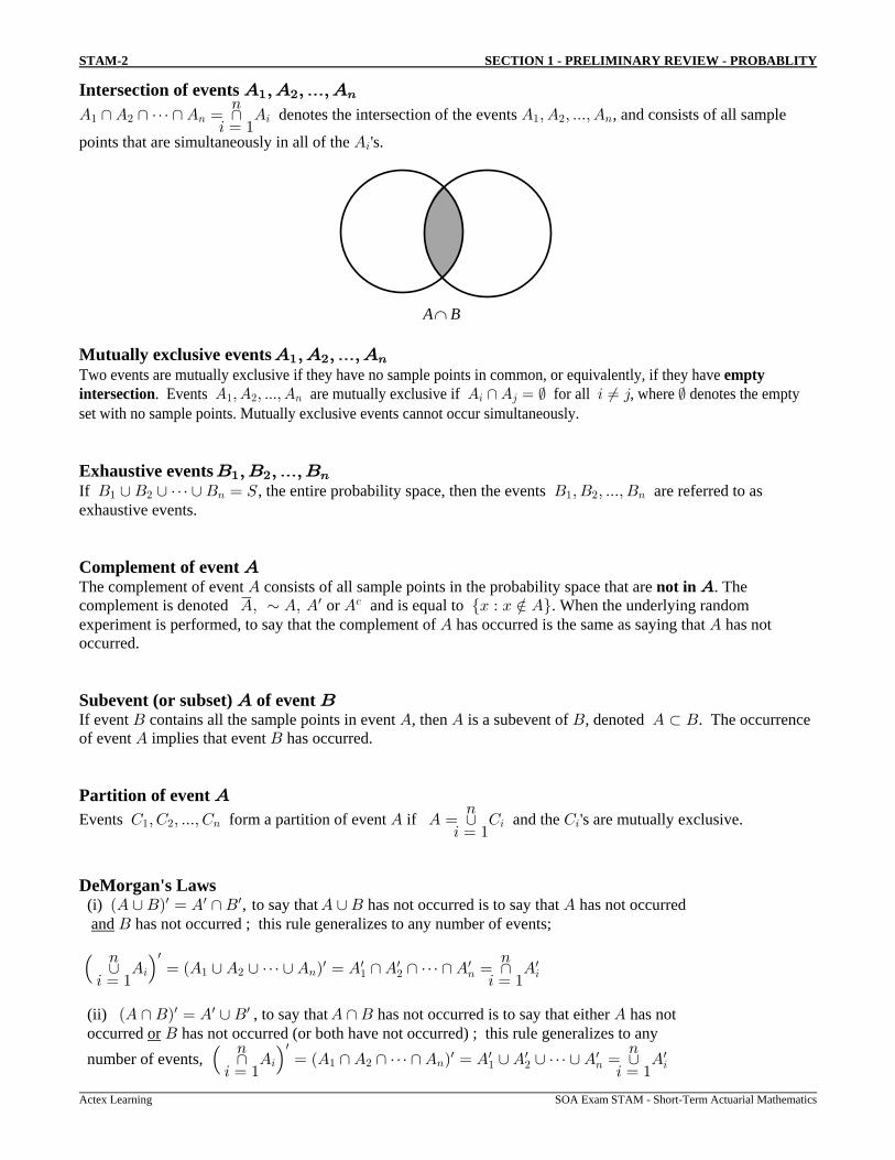
Intersection of events E ßE ß ÞÞÞßE" # 8
E ∩ E ∩â∩E œ ∩ E E ßE ß ÞÞÞß E3 œ "
8" # 8 3 " # 8 denotes the intersection of the events , and consists of all sample
points that are simultaneously in all of the 's.E3
A B Mutually exclusive eventsE ßE ß ÞÞÞßE" # 8
Two events are mutually exclusive if they have no sample points in common, or equivalently, if they have emptyintersection. Events are mutually exclusive if for all , where denotes the emptyE ßE ß ÞÞÞß E E ∩ E œ g 3 Á 4 g" # 8 3 4
set with no sample points. Mutually exclusive events cannot occur simultaneously.
Exhaustive eventsF ßF ß ÞÞÞßF" # 8
If , the entire probability space, then the events are referred to asF ∪ F ∪â∪F œ W F ßF ß ÞÞÞß F" # 8 " # 8
exhaustive events.
Complement of event EThe complement of event consists of all sample points in the probability space that are . TheE not in Ecomplement is denoted or and is equal to . When the underlying randomEß µ Eß E E ÖB À B Â E×
w -
experiment is performed, to say that the complement of has occurred is the same as saying that has notE Eoccurred.
Subevent (or subset) of event E FIf event contains all the sample points in event , then is a subevent of , denoted . The occurrenceF E E F E § Fof event implies that event has occurred.E F
Partition of event EEvents form a partition of event if and the 's are mutually exclusive.G ßG ß ÞÞÞß G E E œ ∪ G G
3 œ "
8" # 8 3 3
DeMorgan's Laws (i) , to say that has not occurred is to say that has not occurredÐE ∪ FÑ œ E ∩ F E ∪ F Ew w w
has not occurred ; this rule generalizes to any number of events;and F
∪ E œ Ð3 œ "
83
w
E ∪ E ∪â∪E Ñ œ E ∩ E ∩â∩E œ ∩ E3 œ "
8" # 8
w w w w w" # 8 3
(ii) , to say that has not occurred is to say that either has notÐE ∩ FÑ œ E ∪ F E ∩ F Ew w w
occurred has not occurred (or both have not occurred) ; this rule generalizes to any or F
number of events, ∩ E œ Ð3 œ "
83
w
E ∩ E ∩â∩E Ñ œ E ∪ E ∪â∪E œ ∪ E3 œ "
8" # 8
w w w w w" # 8 3
SECTION 1 - PRELIMINARY REVIEW - PROBABILITY STAM-3
Actex Learning SOA Exam STAM - Short-Term Actuarial Mathematics
Indicator function for event E
The function is the indicator function for event , where denotes a sample point. is 1M ÐBÑ œ E B M ÐBÑE E
" B−E
! BÂE if
if
if event has occurred.E
Some important rules concerning probability are given below.
(i) if is the entire probability space (when the underlying experiment isT ÒWÓ œ " W performed, some outcome must occur with probability 1).
(ii) (the probability of no face turning up when we toss a die is 0).T ÒgÓ œ !
(iii) If events are mutually exclusive (also called disjoint) thenE ßE ß ÞÞÞß E" # 8
(1.1)T Ò ∪ E Ó œ T ÒE ∪ E ∪â∪E Ó œ T ÒE Ó T ÒE Ó â TÒE Ó œ T ÒE Ó3 œ "
83 " # 8 " # 8 3
3œ"
8
This extends to infinitely many mutually exclusive events.
(iv) For any event , E ! Ÿ T ÒEÓ Ÿ "
(v) If then E § F TÒEÓ Ÿ T ÒFÓ
(vi) For any events , and , (1.2)E F G T ÒE ∪ FÓ œ T ÒEÓ T ÒFÓ T ÒE ∩ FÓ
(vii) For any event , (1.3)E TÒE Ó œ " T ÒEÓw
(viii) For any events and , (1.4)E F TÒEÓ œ T ÒE ∩ FÓ T ÒE ∩ F Ów
(ix) For exhaustive events , (1.5) F ßF ß ÞÞÞß F T Ò ∪ F Ó œ "3 œ "
8" # 8 3
If are exhaustive and mutually exclusive, they form a partition of the entireF ßF ß ÞÞÞß F" # 8
probability space, and for any event ,E
(1.6)T ÒEÓ œ T ÒE ∩ F Ó T ÒE ∩ F Ó â TÒE ∩ F Ó œ T ÒE ∩ F Ó" # 8 33œ"
8(x) The words "percentage" and "proportion" are used as alternatives to "probability". As an example, if we are
told that the percentage or proportion of a group of people that are of a certain type is 20%, this is generallyinterpreted to mean that a randomly chosen person from the group has a 20% probability of being of thattype. This is the "long-run frequency" interpretation of probability. As another example, suppose that we aretossing a fair die. In the long-run frequency interpretation of probability, to say that the probability of tossinga 1 is is the same as saying that if we repeatedly toss the die, the proportion of tosses that are 1's will"
'
approach ."'
STAM-4 SECTION 1 - PRELIMINARY REVIEW - PROBABLITY
Actex Learning SOA Exam STAM - Short-Term Actuarial Mathematics
1.2 Conditional Probability and Independence of Events
Conditional probability arises throughout the STAM Exam material. It is important to be familiar and comfortablewith the definitions and rules of conditional probability.
Conditional probability of event given event E F
If , then is the conditional probability that event occurs given that event TÐFÑ ! E FTÐElFÑ œTÐE∩FÑT ÐFÑ
has occurred. By rewriting the equation we get .TÐE ∩ FÑ œ TÐElFÑ † T ÐFÑ
Partition of a Probability SpaceEvents are said to form a partition of a probability space ifF ßF ß ÞÞÞß F W" # 8
(i) and (ii) for any pair with .F ∪ F ∪â∪F œ W F ∩ F œ g 3 Á 4" # 8 3 4
A partition is a disjoint collection of events which combines to be the full probability space.A simple example of a partition is any event and its complement .F Fw
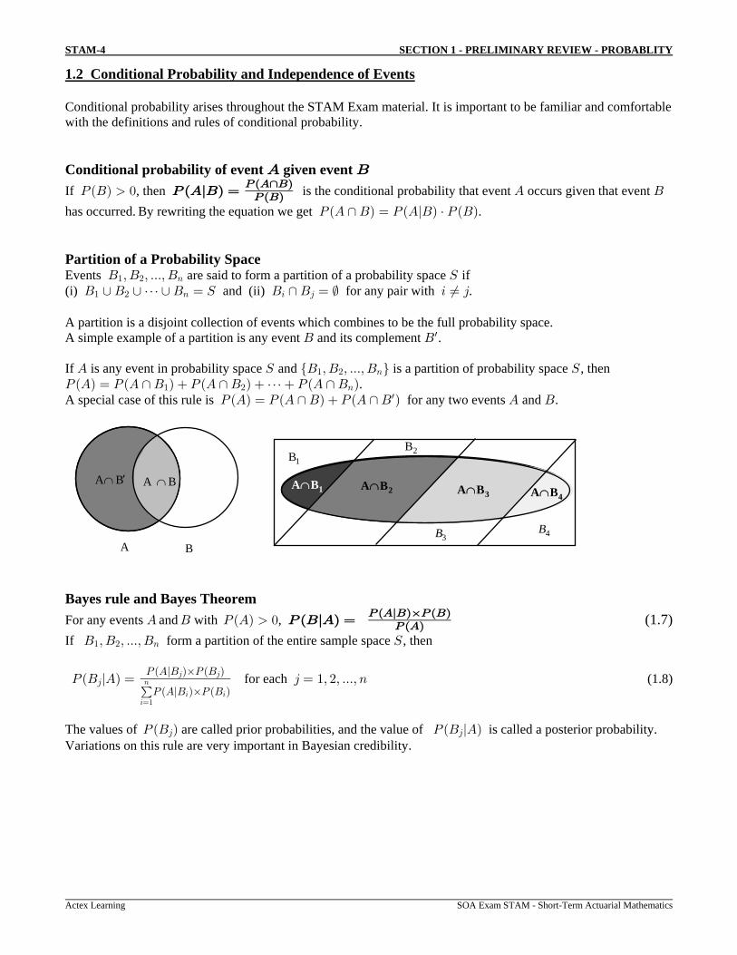
If is any event in probability space and is a partition of probability space , thenE W ÖF ßF ß ÞÞÞß F × W" # 8
T ÐEÑ œ TÐE ∩ F Ñ TÐE ∩ F Ñ â TÐE ∩ F Ñ" # 8 .A special case of this rule is for any two events and .TÐEÑ œ TÐE ∩ FÑ TÐE ∩ F Ñ E Fw
A B
A B A B
1B2B
1A B
3B 4B
2A B3A B
4A B
Bayes rule and Bayes Theorem
For any events and with , E F TÐEÑ ! TÐFlEÑ œ TÐElFÑ‚TÐFÑT ÐEÑ (1.7)
If form a partition of the entire sample space , thenF ßF ß ÞÞÞß F W" # 8
for each (1.8)TÐF lEÑ œ 4 œ "ß #ß ÞÞÞß 84T ÐElF Ñ‚TÐF Ñ
T ÐElF Ñ‚TÐF Ñ
4 4
3œ"
8
3 3
The values of are called prior probabilities, and the value of is called a posterior probability.TÐF Ñ T ÐF lEÑ4 4
Variations on this rule are very important in Bayesian credibility.
SECTION 1 - PRELIMINARY REVIEW - PROBABILITY STAM-5
Actex Learning SOA Exam STAM - Short-Term Actuarial Mathematics
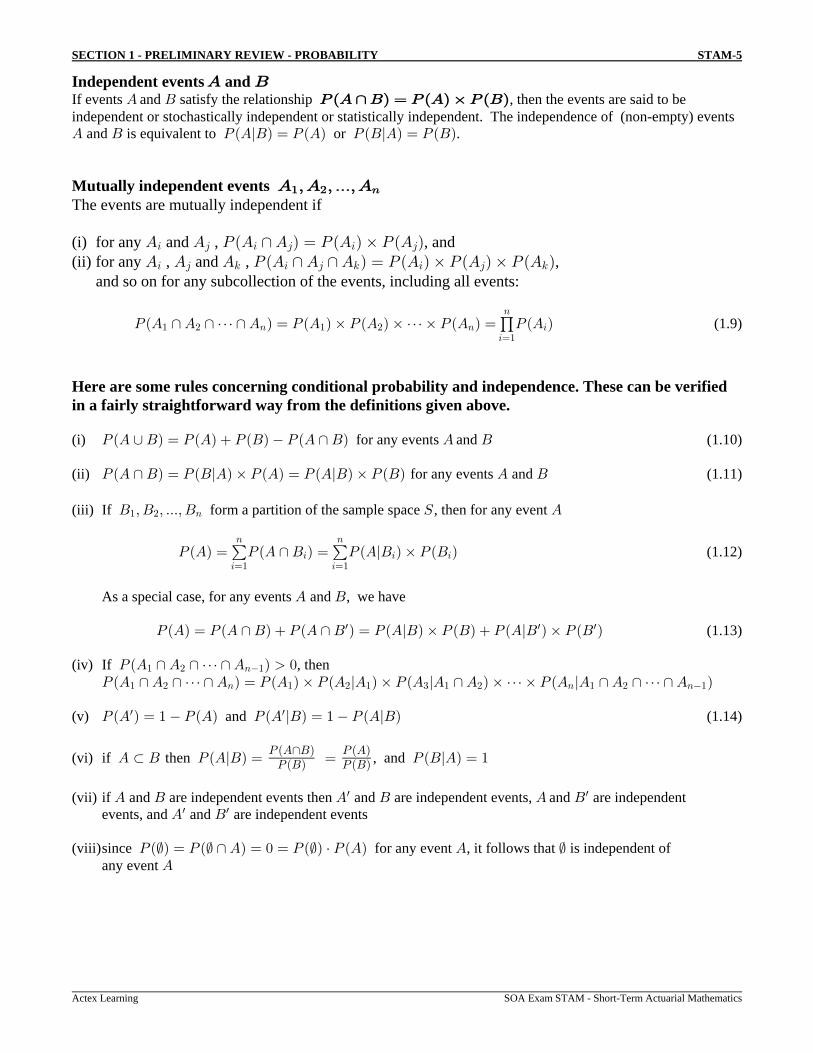
Independent events and E FIf events and satisfy the relationship , then the events are said to beE F TÐE ∩FÑ œ TÐEÑ ‚ TÐFÑindependent or stochastically independent or statistically independent. The independence of (non-empty) eventsE F TÐElFÑ œ TÐEÑ T ÐFlEÑ œ TÐFÑ and is equivalent to or .
Mutually independent events E ßE ß ÞÞÞßE" # 8
The events are mutually independent if
(i) for any and , , andE E TÐE ∩ E Ñ œ TÐE Ñ ‚ TÐE Ñ3 4 3 4 3 4
(ii) for any , and , ,E E E TÐE ∩ E ∩ E Ñ œ TÐE Ñ ‚ TÐE Ñ ‚ TÐE Ñ3 4 5 3 4 5 3 4 5
and so on for any subcollection of the events, including all events:
(1.9)TÐE ∩ E ∩â∩E Ñ œ TÐE Ñ ‚ TÐE Ñ ‚â‚ TÐE Ñ œ TÐE Ñ" # 8 " # 8 33œ"
8
Here are some rules concerning conditional probability and independence. These can be verifiedin a fairly straightforward way from the definitions given above.
(i) for any events and (1.10)TÐE ∪ FÑ œ TÐEÑ TÐFÑ TÐE ∩ FÑ E F
(ii) for any events and (1.11)TÐE ∩ FÑ œ TÐFlEÑ ‚ TÐEÑ œ TÐElFÑ ‚ TÐFÑ E F
(iii) If form a partition of the sample space , then for any event F ßF ß ÞÞÞß F W E" # 8
(1.12)TÐEÑ œ TÐE ∩ F Ñ œ TÐElF Ñ ‚ TÐF Ñ 3œ" 3œ"
8 8
3 3 3
As a special case, for any events and , we haveE F
(1.13)TÐEÑ œ TÐE ∩ FÑ TÐE ∩ F Ñ œ TÐElFÑ ‚ TÐFÑ TÐElF Ñ ‚ TÐF Ñw w w
(iv) If , thenTÐE ∩ E ∩â∩E Ñ !" # 8"
TÐE ∩ E ∩â∩E Ñ œ TÐE Ñ ‚ TÐE lE Ñ ‚ TÐE lE ∩ E Ñ ‚â‚ TÐE lE ∩ E ∩â∩E Ñ" # 8 " # " $ " # 8 " # 8"
(v) and (1.14)TÐE Ñ œ " TÐEÑ T ÐE lFÑ œ " TÐElFÑw w
(vi) if then , and E § F TÐElFÑ œ œ TÐFlEÑ œ "TÐE∩FÑ T ÐEÑT ÐFÑ T ÐFÑ
(vii) if and are independent events then and are independent events, and are independentE F E F E Fw w
events, and and are independent eventsE Fw w
(viii) since for any event , it follows that is independent ofTÐgÑ œ TÐg ∩ EÑ œ ! œ TÐgÑ † T ÐEÑ E g any event E
STAM-6 SECTION 1 - PRELIMINARY REVIEW - PROBABLITY
Actex Learning SOA Exam STAM - Short-Term Actuarial Mathematics
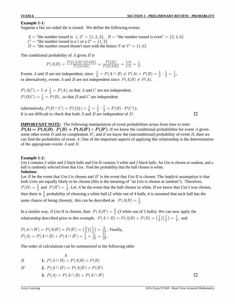
Example 1-1:Suppose a fair six-sided die is tossed. We define the following events:
"the number tossed is " , "the number tossed is even"E œ Ÿ $ œ Ö"ß #ß $× F œ œ Ö#ß %ß '× "the number tossed is a or a "G œ " # œ Ö"ß #× "the number tossed doesn't start with the letters 'f' or 't'"H œ œ Ö"ß '×
The conditional probability of given isE F
TÐElFÑ œ œ œ œTÐÖ"ß#ß$×∩Ö#ß%ß'×Ñ T ÐÖ#×Ñ "Î'
T ÐÖ#ß%ß'×Ñ T ÐÖ#ß%ß'×Ñ "Î# $" .
Events and are not independent, sinceE F œ TÐE ∩ FÑ Á TÐEÑ ‚ TÐFÑ œ œ ," " " "' # # %†
or alternatively, events and are not independent since .E F TÐElFÑ Á TÐEÑ
T ÐElGÑ œ Á œ TÐEÑ E G" "# , so that and are not independent.
TÐFlGÑ œ œ TÐFÑ F G"# , so that and are independent
(alternatively, ).TÐF ∩ GÑ œ TÐÖ#×Ñ œ œ œ TÐFÑ † T ÐGÑ" " "' # $†
It is not difficult to check that both and are independent of . E F H
IMPORTANT NOTE: The following manipulation of event probabilities arises from time to time:T E œ T ElF † T ÐFÑ T ElF TÐF Ñ( ) ( ) ( )w w‚ E. If we know the conditional probabilities for event givensome other event and its complement , and if we know the (unconditional) probability of event , then weF F Fw
can find the probability of event . One of the important aspects of applying this relationship is the determinationEof the appropriate events and .E F
Example 1-2:Urn I contains 2 white and 2 black balls and Urn II contains 3 white and 2 black balls. An Urn is chosen at random, and aball is randomly selected from that Urn. Find the probability that the ball chosen is white.Solution:Let be the event that Urn I is chosen and is the event that Urn II is chosen. The implicit assumption is thatF Fw
both Urns are equally likely to be chosen (this is the meaning of "an Urn is chosen at random"). Therefore,TÐFÑ œ TÐF Ñ œ E" "
# #and Let be the event that the ball chosen in white. If we know that Urn I was chosen,w .
then there is probability of choosing a white ball (2 white out of 4 balls, it is assumed that each ball has the "#
same chance of being chosen); this can be described as .TÐElFÑ œ "#
In a similar way, if Urn II is chosen, then (3 white out of 5 balls). We can now apply theTÐElF Ñ œw $&
relationship described prior to this example. , andTÐE ∩ FÑ œ TÐElFÑ T ÐFÑ œ œ‚ Ð ÑÐ Ñ" " "# # %
T ÐE ∩ F Ñ œ TÐElF Ñ T ÐF Ñ œ œw w w‚ Ð ÑÐ Ñ$ " $& # "! . Finally,
TÐEÑ œ TÐE ∩ FÑ TÐE ∩ F Ñ œ œw " $ ""% "! #! .
The order of calculations can be summarized in the following table EF TÐE ∩ FÑ œ TÐElFÑ ‚ TÐFÑ 1.
Fw 2. TÐE ∩ F Ñ œ TÐElF Ñ ‚ TÐF Ñw w w
3. TÐEÑ œ TÐE ∩ FÑ TÐE ∩ F Ñw
SECTION 1 - PRELIMINARY REVIEW - PROBABILITY STAM-7
Actex Learning SOA Exam STAM - Short-Term Actuarial Mathematics
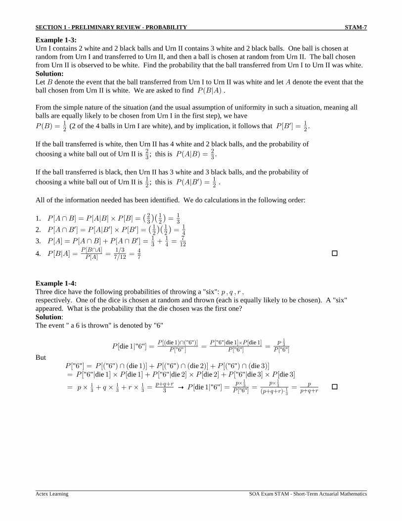
Example 1-3:Urn I contains 2 white and 2 black balls and Urn II contains 3 white and 2 black balls. One ball is chosen atrandom from Urn I and transferred to Urn II, and then a ball is chosen at random from Urn II. The ball chosenfrom Urn II is observed to be white. Find the probability that the ball transferred from Urn I to Urn II was white.Solution:Let denote the event that the ball transferred from Urn I to Urn II was white and let denote the event that theF Eball chosen from Urn II is white. We are asked to find .TÐFlEÑ
From the simple nature of the situation (and the usual assumption of uniformity in such a situation, meaning allballs are equally likely to be chosen from Urn I in the first step), we have
TÐFÑ œ T ÒF Ó œ" "# # (2 of the 4 balls in Urn I are white), and by implication, it follows that .w
If the ball transferred is white, then Urn II has 4 white and 2 black balls, and the probability ofchoosing a white ball out of Urn II is ; this is . # #
$ $T ÐElFÑ œ
If the ball transferred is black, then Urn II has 3 white and 3 black balls, and the probability ofchoosing a white ball out of Urn II is ; this is . " "
# #T ÐElF Ñ œw
All of the information needed has been identified. We do calculations in the following order:
1. T ÒE ∩ FÓ œ T ÒElFÓ T ÒFÓ œ œ‚ Ð ÑÐ Ñ# " "$ # $
2. T ÒE ∩ F Ó œ T ÒElF Ó T ÒF Ó œ œw w w‚ Ð ÑÐ Ñ" " "# # %
3. T ÒEÓ œ T ÒE ∩ FÓ T ÒE ∩ F Ó œ œw " " ($ % "#
4. T ÒFlEÓ œ œ œTÒF∩EÓ "Î$T ÒEÓ (Î"# (
%
Example 1-4:Three dice have the following probabilities of throwing a "six": : ß ; ß < ßrespectively. One of the dice is chosen at random and thrown (each is equally likely to be chosen). A "six"appeared. What is the probability that the die chosen was the first one?Solution:The event " a 6 is thrown" is denoted by "6"
T Ò "l ' Ó œ œ œdie " "T ÒÐ "Ñ∩Ð ' ÑÓ T Ò ' l "Ó T Ò "Ó
T Ò ' Ó T Ò ' Ó T Ò ' Ó
:†die " " " " die die" " " " " "
‚"$
But " " " " die " " die " " dieT Ò ' Ó œ T ÒÐ ' Ñ ∩ Ð "ÑÓ T ÒÐ ' Ñ ∩ Ð #ÑÓ T ÒÐ ' Ñ ∩ Ð $ÑÓ " " die die " " die die " " die dieœ TÒ ' l "Ó ‚ T Ò "Ó T Ò ' l #Ó ‚ T Ò #Ó T Ò ' l $Ó ‚ T Ò $Ó
die " " œ : ‚ ; ‚ < ‚ œ p T Ò "l ' Ó œ œ œ" " "$ $ $
‚ ‚:;< :$ T Ò ' Ó :;<
: :
Ð:;<ц
" "$ $
"$
" "

STAM-8 SECTION 1 - PRELIMINARY REVIEW - PROBABLITY
Actex Learning SOA Exam STAM - Short-Term Actuarial Mathematics
SECTION 1 PROBLEM SET STAM-9
Actex Learning SOA Exam STAM - Short-Term Actuarial Mathematics
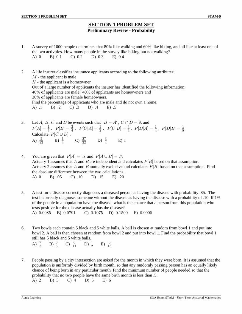
SECTION 1 PROBLEM SETPreliminary Review - Probability
1. A survey of 1000 people determines that 80% like walking and 60% like biking, and all like at least one ofthe two activities. How many people in the survey like biking but not walking?
A) 0 B) 0.1 C) 0.2 D) 0.3 E) 0.4
2. A life insurer classifies insurance applicants according to the following attributes: - the applicant is maleQ - the applicant is a homeownerL Out of a large number of applicants the insurer has identified the following information: 40% of applicants are male, 40% of applicants are homeowners and 20% of applicants are female homeowners. Find the percentage of applicants who are male and do not own a home. A) .1 B) .2 C) .3 D) .4 E) .5
3. Let and be events such that , andEß Fß G H F œ E ß G ∩ H œ gw
, , , , , T ÒEÓ œ T ÒFÓ œ T ÒGlEÓ œ T ÒGlFÓ œ T ÒHlEÓ œ T ÒHlFÓ œ" $ " $ " "% % # % % )
Calculate .T ÒG ∪ HÓ
A) B) C) D) E)& " #( $$# % $# % "
4. You are given that and .T ÒEÓ œ Þ& T ÒE ∪ FÓ œ Þ( Actuary 1 assumes that and are independent and calculates based on that assumption.E F TÒFÓ Actuary 2 assumes that and mutually exclusive and calculates based on that assumption. FindE F TÒFÓ
the absolute difference between the two calculations. A) 0 B) .05 C) .10 D) .15 E) .20
5. A test for a disease correctly diagnoses a diseased person as having the disease with probability .85. Thetest incorrectly diagnoses someone without the disease as having the disease with a probability of .10. If 1%of the people in a population have the disease, what is the chance that a person from this population whotests positive for the disease actually has the disease?
A) B) C) D) E) !Þ!!)& !Þ!(*" !Þ"!(& !Þ"&!! !Þ*!!!
6. Two bowls each contain 5 black and 5 white balls. A ball is chosen at random from bowl 1 and put intobowl 2. A ball is then chosen at random from bowl 2 and put into bowl 1. Find the probability that bowl 1still has 5 black and 5 white balls.
A) B) C) D) E) # $ ' " '$ & "" # "$
7. People passing by a city intersection are asked for the month in which they were born. It is assumed that thepopulation is uniformly divided by birth month, so that any randomly passing person has an equally likelychance of being born in any particular month. Find the minimum number of people needed so that theprobability that no two people have the same birth month is less than .5.
A) 2 B) 3 C) 4 D) 5 E) 6
STAM-10 SECTION 1 PROBLEM SET
Actex Learning SOA Exam STAM - Short-Term Actuarial Mathematics
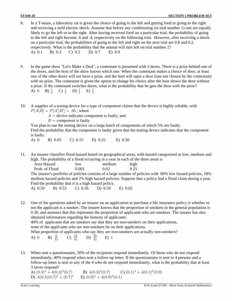
8. In a T-maze, a laboratory rat is given the choice of going to the left and getting food or going to the rightand receiving a mild electric shock. Assume that before any conditioning (in trial number 1) rats are equallylikely to go the left or to the right. After having received food on a particular trial, the probability of goingto the left and right become .6 and .4, respectively on the following trial. However, after receiving a shockon a particular trial, the probabilities of going to the left and right on the next trial are 0.8 and 0.2,respectively. What is the probability that the animal will turn left on trial number 2?
A) 0.1 B) 0.3 C) 0.5 D) 0.7 E) 0.9
9. In the game show "Let's Make a Deal", a contestant is presented with 3 doors. There is a prize behind one ofthe doors, and the host of the show knows which one. When the contestant makes a choice of door, at leastone of the other doors will not have a prize, and the host will open a door (one not chosen by the contestant)with no prize. The contestant is given the option to change his choice after the host shows the door withouta prize. If the contestant switches doors, what is the probability that he gets the door with the prize?
A) B) C) D) E)! " " " #' $ # $
10. A supplier of a testing device for a type of component claims that the device is highly reliable, withT ÒElFÓ œ T ÒE lF Ó œ Þ*&w w , where
device indicates component is faulty, andE œ component is faulty .F œ You plan to use the testing device on a large batch of components of which 5% are faulty. Find the probability that the component is faulty given that the testing device indicates that the component
is faulty . A) 0 B) 0.05 C) 0.15 D) 0.25 E) 0.50
11. An insurer classifies flood hazard based on geographical areas, with hazard categorized as low, medium andhigh. The probability of a flood occurring in a year in each of the three areas is
Area Hazard low medium high Prob. of Flood 0.001 0.02 0.25 The insurer's portfolio of policies consists of a large number of policies with 80% low hazard policies, 18%
medium hazard policies and 2% high hazard policies. Suppose that a policy had a flood claim during a year.Find the probability that it is a high hazard policy.
A) 0.50 B) 0.53 C) 0.56 D) 0.59 E) 0.62
12. One of the questions asked by an insurer on an application to purchase a life insurance policy is whether ornot the applicant is a smoker. The insurer knows that the proportion of smokers in the general population is0.30, and assumes that this represents the proportion of applicants who are smokers. The insurer has alsoobtained information regarding the honesty of applicants:
40% of applicants that are smokers say that they are non-smokers on their applications, none of the applicants who are non-smokers lie on their applications. What proportion of applicants who say they are non-smokers are actually non-smokers? A) B) C) D) E) ! "' "# $&
%" %" %"
13. When sent a questionnaire, 50% of the recipients respond immediately. Of those who do not respondimmediately, 40% respond when sent a follow-up letter. If the questionnaire is sent to 4 persons and afollow-up letter is sent to any of the 4 who do not respond immediately, what is the probability that at least3 never respond?
A) B) C) Ð!Þ$Ñ %Ð!Þ$Ñ Ð!Þ(Ñ %Ð!Þ$Ñ Ð!Þ(Ñ Ð!Þ"Ñ %Ð!Þ"Ñ Ð!Þ*Ñ% $ $ % $
D) E) Þ%Ð!Þ$ÑÐ!Þ(Ñ Ð!Þ(Ñ Ð!Þ*Ñ %Ð!Þ*Ñ Ð!Þ"Ñ$ % % $
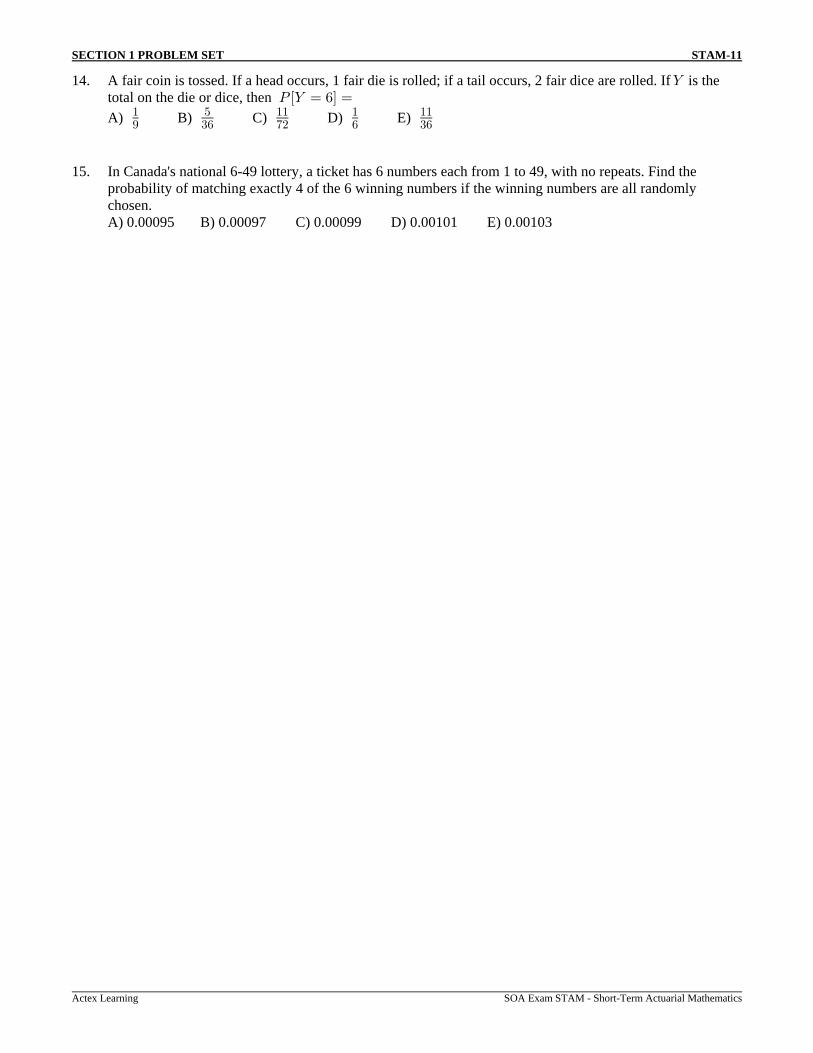
SECTION 1 PROBLEM SET STAM-11
Actex Learning SOA Exam STAM - Short-Term Actuarial Mathematics
14. A fair coin is tossed. If a head occurs, 1 fair die is rolled; if a tail occurs, 2 fair dice are rolled. If is the]total on the die or dice, then T Ò] œ 'Ó œ
A) B) C) D) E) " & "" " ""* $' (# ' $'
15. In Canada's national 6-49 lottery, a ticket has 6 numbers each from 1 to 49, with no repeats. Find theprobability of matching exactly 4 of the 6 winning numbers if the winning numbers are all randomlychosen.
A) 0.00095 B) 0.00097 C) 0.00099 D) 0.00101 E) 0.00103
STAM-12 SECTION 1 PROBLEM SET
Actex Learning SOA Exam STAM - Short-Term Actuarial Mathematics
SECTION 1 PROBLEM SET SOLUTIONS
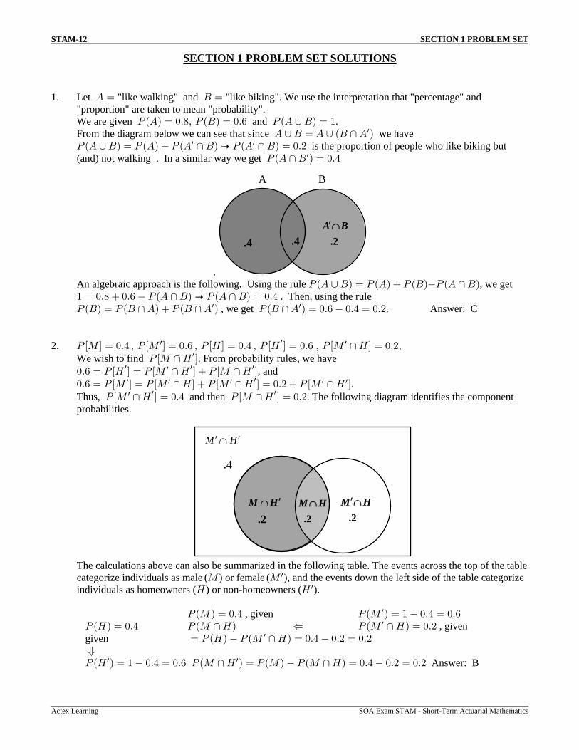
1. Let "like walking" and "like biking". We use the interpretation that "percentage" andE œ F œ"proportion" are taken to mean "probability".
We are given and .TÐEÑ œ !Þ)ß T ÐFÑ œ !Þ' T ÐE ∪ FÑ œ " From the diagram below we can see that since we haveE ∪ F œ E ∪ ÐF ∩ E Ñw
is the proportion of people who like biking butTÐE ∪ FÑ œ TÐEÑ TÐE ∩ FÑ p TÐE ∩ FÑ œ !Þ#w w
(and) not walking . In a similar way we get TÐE ∩ F Ñ œ !Þ%w
.4 .2
A B.4
BA
. An algebraic approach is the following. Using the rule , we getTÐE ∪ FÑ œ TÐEÑ TÐFÑTÐE ∩ FÑ
" œ !Þ) !Þ' TÐE ∩ FÑ p TÐE ∩ FÑ œ !Þ% . Then, using the rule , we get . Answer: CTÐFÑ œ TÐF ∩ EÑ TÐF ∩ E Ñ TÐF ∩ E Ñ œ !Þ' !Þ% œ !Þ#w w
2. T ÒQÓ œ !Þ% ß T ÒQ Ó œ !Þ' ß T ÒLÓ œ !Þ% ß T ÒL Ó œ !Þ' ß T ÒQ ∩LÓ œ !Þ#ßw ww
We wish to find . From probability rules, we haveT ÒQ ∩L Ów
, and!Þ' œ T ÒL Ó œ T ÒQ ∩L Ó T ÒQ ∩L Ów w ww
!Þ' œ T ÒQ Ó œ T ÒQ ∩LÓ T ÒQ ∩L Ó œ !Þ# T ÒQ ∩L Ów w w w ww . Thus, and then . The following diagram identifies the componentT ÒQ ∩L Ó œ !Þ% T ÒQ ∩L Ó œ !Þ#w w w
probabilities.
.2 .2
M HM H
.2
M H
.4
M H
The calculations above can also be summarized in the following table. The events across the top of the tablecategorize individuals as male ( ) or female ( ), and the events down the left side of the table categorizeQ Qw
individuals as homeowners ( ) or non-homeowners ( ).L Lw
, given TÐQÑ œ !Þ% T ÐQ Ñ œ " !Þ% œ !Þ'w
, givenTÐLÑ œ !Þ% T ÐQ ∩LÑ É TÐQ ∩LÑ œ !Þ#w
given œ TÐLÑ TÐQ ∩LÑ œ !Þ% !Þ# œ !Þ#w
Ì Answer: BTÐL Ñ œ " !Þ% œ !Þ' T ÐQ ∩L Ñ œ TÐQÑ TÐQ ∩LÑ œ !Þ% !Þ# œ !Þ#w w
SECTION 1 PROBLEM SET STAM-13
Actex Learning SOA Exam STAM - Short-Term Actuarial Mathematics
3. Since and have empty intersection, G H TÒG ∪ HÓ œ T ÒGÓ T ÒHÓÞ
Also, since and are "exhaustive" events (since they are complementary events, their union is the entireE Fsample space, with a combined probability of
T ÒE ∪ FÓ œ T ÒEÓ T ÒFÓ œ " ).
We use the rule , and the rule to getT ÒGÓ œ T ÒG ∩ EÓ T ÒG ∩ E Ó T ÒGlEÓ œw T ÒE∩GÓT ÒEÓ
andT ÒGÓ œ T ÒGlEÓ ‚ T ÒEÓ T ÒGlE Ó ‚ T ÒE Ó œ ‚ ‚ œw w " " $ $ ""# % % % "'
T ÒHÓ œ T ÒHlEÓ ‚ T ÒEÓ T ÒHlE Ó ‚ T ÒE Ó œ ‚ ‚ œ Þw w " " " $ &% % ) % $#
Then, Answer: C.T ÒG ∪ HÓ œ T ÒGÓ T ÒHÓ œ Þ#($#
4. Actuary 1: Since and are independent, so are and .E F E Fw w
.T ÒE ∩ F Ó œ " T ÒE ∪ FÓ œ !Þ$w w
But .!Þ$ œ T ÒE ∩ F Ó œ T ÒE Ó † T ÒF Ó œ Ð!Þ&ÑT ÒF Ó p T ÒF Ó œ !Þ' p T ÒFÓ œ !Þ%w w w w w w
Actuary 2: .!Þ( œ T ÒE ∪ FÓ œ T ÒEÓ T ÒFÓ œ !Þ& T ÒFÓ p T ÒFÓ œ !Þ# Absolute difference is . Answer: E l!Þ% Þ#l œ !Þ#
5. We define the following events: - a person has the disease,H - a person tests positive for the disease. We are given and andXT T ÒXT lHÓ œ Þ)& T ÒXT lH Ó œ Þ"!w
T ÒHÓ œ Þ!" T ÒHlXT Ó. We wish to find .
Using the formulation for conditional probability we have .T ÒHlXT Ó œT ÒH∩XT ÓT ÒXT Ó
But , andT ÒH ∩ XT Ó œ T ÒXT lHÓ ‚ T ÒHÓ œ Ð!Þ)&ÑÐ!Þ!"Ñ œ !Þ!!)& . Then,T ÒH ∩ XT Ó œ T ÒXT lH Ó ‚ T ÒH Ó œ Ð!Þ"!ÑÐ!Þ**Ñ œ !Þ!**w w w
.T ÒXT Ó œ T ÒH ∩ XT Ó T ÒH ∩ XT Ó œ Þ"!(& p T ÒHlXT Ó œ œ !Þ!(*"w !Þ!!)&!Þ"!(&
The following table summarizes the calculations.
, given T ÒHÓ œ !Þ!" Ê TÒH Ó œ " T ÒHÓ œ !Þ**w
Ì Ì T ÒH ∩ XT Ó T ÒH ∩ XT Ów
œ TÒXT lHÓ ‚ T ÒHÓ œ !Þ!!)& œ T ÒXT lH Ó ‚ T ÒH Ó œ !Þ!**w w
Ì T ÒXT Ó œ T ÒH ∩ XT Ó T ÒH ∩ XT Ó œ !Þ"!(&w
Ì
. Answer: BT ÒHlXT Ó œ œ œ !Þ!(*"T ÒH∩XT ÓT ÒXT Ó Þ"!(&
Þ!!)&
STAM-14 SECTION 1 PROBLEM SET
Actex Learning SOA Exam STAM - Short-Term Actuarial Mathematics
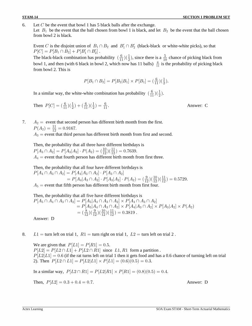
6. Let be the event that bowl 1 has 5 black balls after the exchange.G Let be the event that the ball chosen from bowl 1 is black, and let be the event that the ball chosenF F" #
from bowl 2 is black.
Event is the disjoint union of and (black-black or white-white picks), so thatG F ∩ F F ∩ F" # " #w w
T ÒGÓ œ T ÒF ∩ F Ó T ÒF ∩ F Ó" # " #w w .
The black-black combination has probability , since there is a chance of picking black fromÐ ÑÐ Ñ' " &"" # "!
bowl 1, and then (with 6 black in bowl 2, which now has 11 balls) is the probability of picking black'""
from bowl 2. This is
T ÒF ∩ F Ó œ T ÒF lF Ó ‚ T ÒF Ó œ Ð ÑÐ Ñ" # # " "' """ # .
In a similar way, the white-white combination has probability .Ð ÑÐ Ñ' """ #
Then . Answer: CT ÒGÓ œ Ð ÑÐ Ñ Ð ÑÐ Ñ œ' " ' " '"" # "" # ""
7. event that second person has different birth month from the first.E œ#
TÐE Ñ œ œ !Þ*"'(Þ#"""#
event that third person has different birth month from first and second.E œ$
Then, the probability that all three have different birthdays is .T ÒE ∩ E Ó œ T ÒE lE Ó † T ÐE Ñ œ Ð ÑÐ Ñ œ !Þ('$*$ # $ # #
"! """# "#
event that fourth person has different birth month from first three.E œ%
Then, the probability that all four have different birthdays is T ÒE ∩ E ∩ E Ó œ T ÒE lE ∩ E Ó † T ÒE ∩ E Ó% $ # % $ # $ #
.œ TÒE lE ∩ E Ó † T ÒE lE Ó † T ÐE Ñ œ Ð ÑÐ ÑÐ Ñ œ !Þ&(#*% $ # $ # #* "! """# "# "#
event that fifth person has different birth month from first four.E œ&
Then, the probability that all five have different birthdays is T ÒE ∩ E ∩ E ∩ E Ó œ T ÒE lE ∩ E ∩ E Ó ‚ T ÒE ∩ E ∩ E Ó& % $ # & % $ # % $ #
œ TÒE lE ∩ E ∩ E Ó ‚ T ÒE lE ∩ E Ó ‚ T ÒE lE Ó ‚ TÐE Ñ& % $ # % $ # $ # #
. œ Ð ÑÐ ÑÐ ÑÐ Ñ œ !Þ$)"*) * "! """# "# "# "#
Answer: D
8. turn left on trial 1, turn right on trial 1, turn left on trial 2 .P" œ V" œ P# œ
We are given that .T ÒP"Ó œ T ÒV"Ó œ !Þ& since form a partition .T ÒP#Ó œ T ÒP# ∩ P"Ó T ÒP# ∩ V"Ó P"ßV" (if the rat turns left on trial 1 then it gets food and has a 0.6 chance of turning left on trialT ÒP#lP"Ó œ !Þ'
2). Then .T ÒP# ∩ P"Ó œ T ÒP#lP"Ó ‚ T ÒP"Ó œ Ð!Þ'ÑÐ!Þ&Ñ œ !Þ$
In a similar way, .T ÒP# ∩ V"Ó œ T ÒP#lV"Ó ‚ T ÒV"Ó œ Ð!Þ)ÑÐ!Þ&Ñ œ !Þ%
Then, . Answer: DT ÒP#Ó œ !Þ$ !Þ% œ !Þ(
SECTION 1 PROBLEM SET STAM-15
Actex Learning SOA Exam STAM - Short-Term Actuarial Mathematics
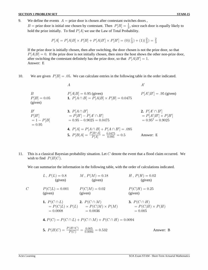
9. We define the events prize door is chosen after contestant switches doors ,E œ
prize door is initial one chosen by contestant. Then , since each door is equally likely toF œ TÒFÓ œ "$
hold the prize initially. To find we use the Law of Total Probability.T ÒEÓ
T ÒEÓ œ T ÒElFÓ ‚ T ÒFÓ T ÒElF Ó ‚ T ÒF Ó œ Ð!ÑÐ Ñ Ð"ÑÐ Ñ œw w " # #$ $ $
If the prize door is initially chosen, then after switching, the door chosen is not the prize door, so thatT ÒElFÓ œ !. If the prize door is not initially chosen, then since the host shows the other non-prize door,after switching the contestant definitely has the prize door, so that .T ÒElF Ó œ "w
Answer: E
10. We are given . We can calculate entries in the following table in the order indicated.T ÒFÓ œ Þ!&
E Ew
(given) (given)F TÒElFÓ œ !Þ*& T ÒE lF Ó œ Þ*&w w
T ÒFÓ œ !Þ!& T ÒE ∩ FÓ œ T ÒElFÓ ‚ T ÒFÓ œ !Þ!%(&1. (given)
F TÒE ∩ F Ó T ÒE ∩ F Ów w w w3. 2. T ÒF Ó œ T ÒF Ó T ÒE ∩ F Ó œ T ÒE lF Ó ‚ T ÒF Ów w w w w w w
œ " T ÒFÓ œ !Þ*& !Þ*!#& œ !Þ!%(& œ !Þ*& œ !Þ*!#&#
œ !Þ*& 4. T ÒEÓ œ T ÒE ∩ FÓ T ÒE ∩ F Ó œ Þ!*&w
5. T ÒFlEÓ œ œ œ !Þ&T ÒF∩EÓT ÒEÓ !Þ!*&
!Þ!%(& Answer: E
11. This is a classical Bayesian probability situation. Let denote the event that a flood claim occurred. WeGwish to find .TÐLlGÑ
We can summarize the information in the following table, with the order of calculations indicated.
P ß T ÐPÑ œ !Þ) Q ß T ÐQÑ œ !Þ") L ß T ÐLÑ œ !Þ!# (given) (given) (given)
G TÐGlPÑ œ !Þ!!" T ÐGlQÑ œ !Þ!# T ÐGlLÑ œ !Þ#& (given) (given) (given)
1. 2. 3.TÐG ∩ PÑ TÐG ∩QÑ TÐG ∩ LÑ œ TÐGlPÑ ‚ TÐPÑ œ TÐGlQÑ ‚ TÐQÑ œ TÐGlLÑ ‚ TÐLÑ œ !Þ!!!) œ !Þ!!$' œ !Þ!!&
4. TÐGÑ œ TÐG ∩ PÑ TÐG ∩QÑ TÐG ∩ LÑ œ !Þ!!*%
5. Answer: BTÐLlGÑ œ œ œ !Þ&$#TÐL∩GÑT ÐGÑ !Þ!!*%
!Þ!!&
STAM-16 SECTION 1 PROBLEM SET
Actex Learning SOA Exam STAM - Short-Term Actuarial Mathematics
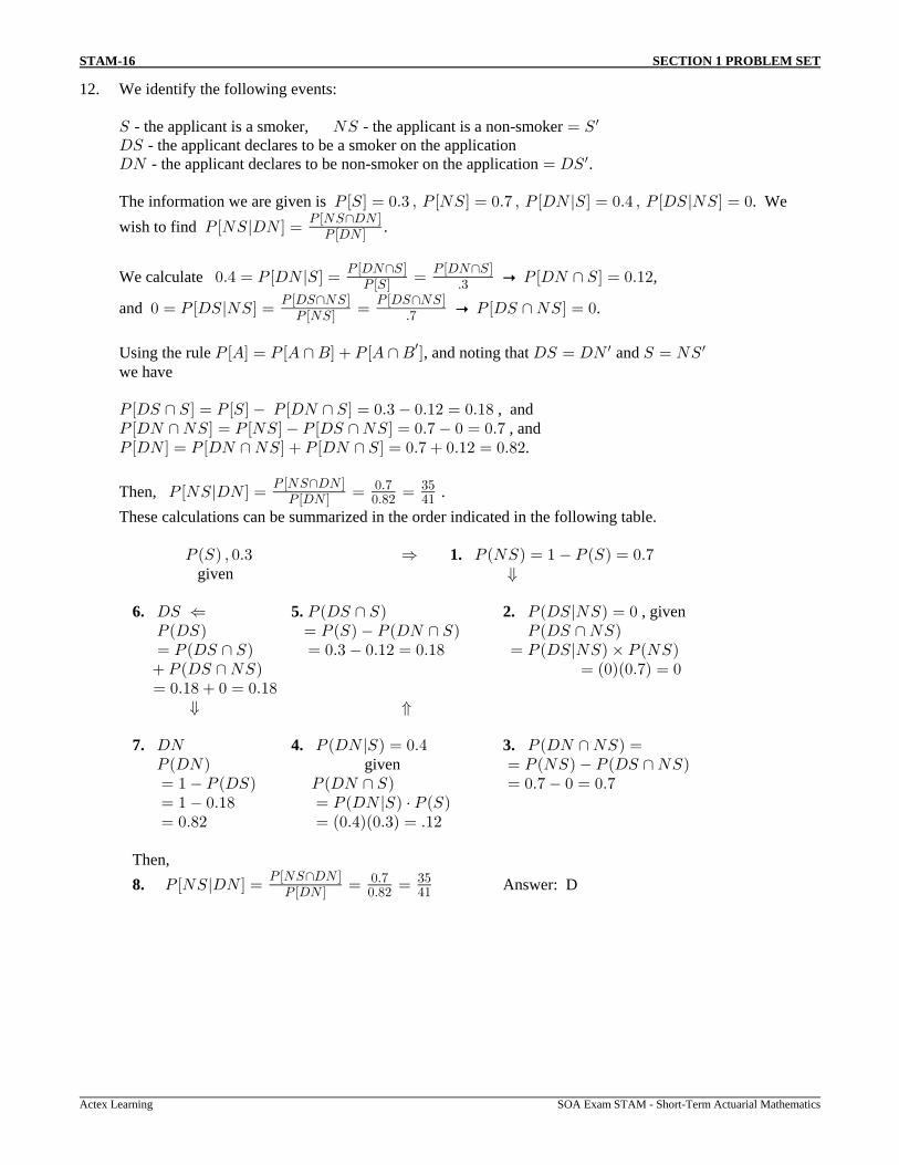
12. We identify the following events:
- the applicant is a smoker, - the applicant is a non-smokerW RW œ Ww
- the applicant declares to be a smoker on the applicationHW - the applicant declares to be non-smoker on the application .HR œ HWw
The information we are given is . WeT ÒWÓ œ !Þ$ ß T ÒRWÓ œ !Þ( ß T ÒHRlWÓ œ !Þ% ß T ÒHWlRWÓ œ !
wish to find .T ÒRWlHRÓ œT ÒRW∩HRÓ
T ÒHRÓ
We calculate ,!Þ% œ T ÒHRlWÓ œ œ p T ÒHR ∩ WÓ œ !Þ"#T ÒHR∩WÓ T ÒHR∩WÓ
T ÒWÓ Þ$
and .! œ T ÒHWlRWÓ œ œ p T ÒHW ∩ RWÓ œ !T ÒHW∩RWÓ T ÒHW∩RWÓ
T ÒRWÓ Þ(
Using the rule , and noting that and T ÒEÓ œ T ÒE ∩ FÓ T ÒE ∩ F Ó HW œ HR W œ RWw w w
we have
, andT ÒHW ∩ WÓ œ T ÒWÓ T ÒHR ∩ WÓ œ !Þ$ !Þ"# œ !Þ") , andT ÒHR ∩RWÓ œ T ÒRWÓ T ÒHW ∩ RWÓ œ !Þ( ! œ !Þ( .T ÒHRÓ œ T ÒHR ∩RWÓ T ÒHR ∩ WÓ œ !Þ( !Þ"# œ !Þ)#
Then, . T ÒRWlHRÓ œ œ œTÒRW∩HRÓ
T ÒHRÓ !Þ)# %"!Þ( $&
These calculations can be summarized in the order indicated in the following table.
TÐWÑ ß !Þ$ Ê TÐRWÑ œ " TÐWÑ œ !Þ(1. given Ì
6. 5. 2. HW É TÐHW ∩ WÑ T ÐHWlRWÑ œ ! , given TÐHWÑ œ TÐWÑ TÐHR ∩ WÑ TÐHW ∩ RWÑ œ TÐHW ∩ WÑ œ !Þ$ !Þ"# œ !Þ") œ TÐHWlRWÑ ‚ TÐRWÑ TÐHW ∩ RWÑ œ Ð!ÑÐ!Þ(Ñ œ ! œ !Þ") ! œ !Þ") Ì Ë
7. 4. 3. HR TÐHRlWÑ œ !Þ% T ÐHR ∩RWÑ œ given TÐHRÑ œ TÐRWÑ TÐHW ∩ RWÑ œ " TÐHWÑ TÐHR ∩ WÑ œ !Þ( ! œ !Þ( œ " !Þ") œ TÐHRlWÑ † T ÐWÑ œ !Þ)# œ Ð!Þ%ÑÐ!Þ$Ñ œ Þ"#
Then,
8. Answer: DT ÒRWlHRÓ œ œ œTÒRW∩HRÓ
T ÒHRÓ !Þ)# %"!Þ( $&
SECTION 1 PROBLEM SET STAM-17
Actex Learning SOA Exam STAM - Short-Term Actuarial Mathematics
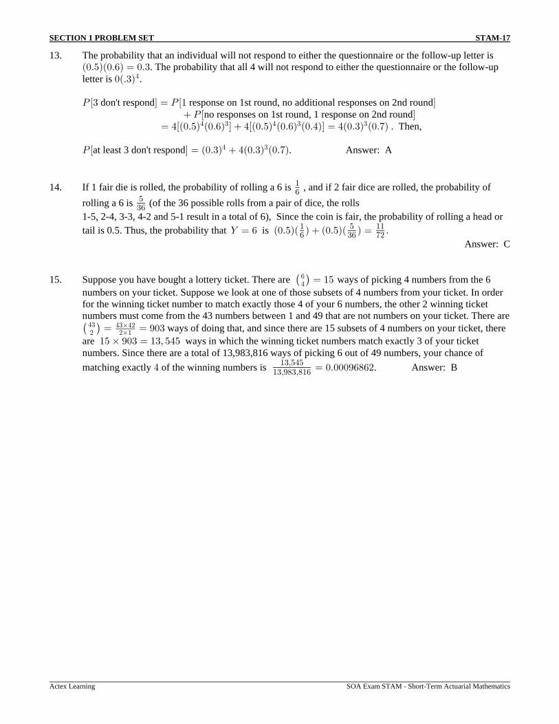
13. The probability that an individual will not respond to either the questionnaire or the follow-up letter isÐ!Þ&ÑÐ!Þ'Ñ œ !Þ$. The probability that all 4 will not respond to either the questionnaire or the follow-upletter is .!ÐÞ$Ñ%
don't respond response on 1st round, no additional responses on 2nd roundT Ò$ Ó œ T Ò" Ó no responses on 1st round, 1 response on 2nd round TÒ Ó . Then,œ %ÒÐ!Þ&Ñ Ð!Þ'Ñ Ó %ÒÐ!Þ&Ñ Ð!Þ'Ñ Ð!Þ%ÑÓ œ %Ð!Þ$Ñ Ð!Þ(Ñ% $ % $ $
at least 3 don't respond . Answer: AT Ò Ó œ Ð!Þ$Ñ %Ð!Þ$Ñ Ð!Þ(Ñ% $
14. If 1 fair die is rolled, the probability of rolling a 6 is , and if 2 fair dice are rolled, the probability of"'
rolling a 6 is (of the 36 possible rolls from a pair of dice, the rolls&$'
1-5, 2-4, 3-3, 4-2 and 5-1 result in a total of 6), Since the coin is fair, the probability of rolling a head ortail is 0.5. Thus, the probability that is ] œ ' Ð!Þ&ÑÐ Ñ Ð!Þ&ÑÐ Ñ œ Þ" & ""
' $' (#Answer: C
15. Suppose you have bought a lottery ticket. There are ways of picking 4 numbers from the 6 '% œ "&
numbers on your ticket. Suppose we look at one of those subsets of 4 numbers from your ticket. In orderfor the winning ticket number to match exactly those 4 of your 6 numbers, the other 2 winning ticketnumbers must come from the 43 numbers between 1 and 49 that are not numbers on your ticket. There are %$
# #‚"%$‚%#œ œ *!$ ways of doing that, and since there are 15 subsets of 4 numbers on your ticket, there
are ways in which the winning ticket numbers match exactly 3 of your ticket"& ‚ *!$ œ "$ß &%&numbers. Since there are a total of 13,983,816 ways of picking 6 out of 49 numbers, your chance of
matching exactly of the winning numbers is . Answer: B% œ !Þ!!!*')'#"$ß&%&
"$ß*)$ß)"'

STAM-18 SECTION 1 PROBLEM SET
Actex Learning SOA Exam STAM - Short-Term Actuarial Mathematics
SECTION 2 - PRELIMINARY REVIEW - RANDOM VARIABLES I STAM-19
Actex Learning SOA Exam STAM - Short-Term Actuarial Mathematics
SECTION 2 - PRELIMINARY REVIEW - RANDOM VARIABLES IProbability, Density and Distribution Functions
This section relates to Chapter 2 of "Loss Models". The suggested time frame for covering this section is twohours. A brief review of some basic calculus relationships is presented first.
2.1 Calculus Review
Natural logarithm and exponential functions68ÐBÑ œ 691ÐBÑ / is the logarithm to the base ;
68Ð/Ñ œ " ß 68Ð"Ñ œ !ß / œ " ß!
68Ð/ Ñ œ C ß / œ Bß 68Ð+ Ñ œ C ‚ 68Ð+Ñ ßC 68ÐBÑ C
68ÐC † DÑ œ 68ÐCÑ 68ÐDÑß 68Ð Ñ œ 68ÐCÑ 68ÐDÑ ßCD
(2.1)/ / œ / ß Ð/ Ñ œ /B D BD B A BA
Differentiation
For the function 0ÐBÑß 0 ÐBÑ œ œw
2Ä!
.0
.B 20ÐB2Ñ0ÐBÑ
lim (2.2)
Product rule: (2.3)..B
w wÒ1ÐBÑ2ÐBÑÓ œ 1 ÐBÑ2ÐBÑ 1ÐBÑ2 ÐBÑ
Quotient rule: (2.4)..B 2ÐBÑ Ò2ÐBÑÓ
1ÐBÑ 2ÐBÑ1 ÐBÑ1ÐBÑ2 ÐBÑÒ Ó œw w
#
Chain rule: (2.5) . . ..B 1ÐBÑ .B .B
1 ÐBÑ68Ò1ÐBÑÓ œ ß Ò1ÐBÑÓ œ 8Ò1ÐBÑÓ ‚ 1 ÐBÑ ß + œ + ‚ 68Ð+Ñ
w8 8" w B B
Integration
B .B œ - ß + .B œ - ß .B œ 68Ò+ ,BÓ -8 BB + " "8" 68Ð+Ñ +,B ,
8" B
‚ (2.6)
Integration by parts : + +
, ,?Ð>Ñ .@Ð>Ñ œ ?Ð,Ñ@Ð,Ñ ?Ð+Ñ@Ð+Ñ @Ð>Ñ .?Ð>Ñ
for definite integrals, and ? .@ œ ?@ @ .?
for indefinite integrals (this is derived by integrating both sides of the product rule); note that
and .@Ð>Ñ œ @ Ð>Ñ .> .?Ð>Ñ œ ? Ð>Ñ .>w w
. ..B .B
+ BB ,1Ð>Ñ .> œ 1ÐBÑ ß 1Ð>Ñ .> œ 1ÐBÑ (2.7)
..B
2ÐBÑ4ÐBÑ w w1Ð>Ñ.> œ 1Ð4ÐBÑÑ ‚ 4 ÐBÑ 1Ð2ÐBÑÑ ‚ 2 ÐBÑ (2.8)
if and is an integer (2.9)!∞ 8 5BB / .B œ 5 ! 8 !8x
58"
STAM-20 SECTION 2 - PRELIMINARY REVIEW - RANDOM VARIABLES I
Actex Learning SOA Exam STAM - Short-Term Actuarial Mathematics
The word "model" used in the context of a loss model, usually refers to the distribution of a loss random variable.Random variables are the basic components used in actuarial modeling. In this section we review the definitionsand illustrate the variety of random variables that we will encounter in the STAM Exam material.
A random variable is a numerical quantity that is related to the outcome of some random experiment on aprobability space. For the most part, the random variables we will encounter are the numerical outcomes of someloss related event such as the dollar amount of claims in one year from an auto insurance policy, or the number oftornados that touch down in Kansas in a one year period.
2.2 Discrete Random VariableThe random variable is discrete and is said to have a if it can take on values only from a\ discrete distributionfinite or countable infinite sequence (usually the integers or some subset of the integers). As an example, considerthe following two random variables related to successive tosses of a coin:
\ œ " \ œ ! if the first head occurs on an even-numbered toss, if the first head occurs on an odd-numberedtoss;
] œ 8 8, where is the number of the toss on which the first head occurs.
Both and are discrete random variables, where can take on only the values or , and can take on any\ ] \ ! " ]positive integer value.
Probability function of a discrete random variableThe probability function (pf) of a discrete random variable is usually denoted or , and is equal to:ÐBÑ Ð 0ÐBÑÑT Ð\ œ BÑ. As its name suggests, the probability function describes the probability of individual outcomesoccurring.
The probability function must satisfy the following two conditions:
(i) for all , and (ii) (2.10)! Ÿ :ÐBÑ Ÿ " B :ÐBÑ œ "B
For the random variable above, the probability function is \ :Ð!Ñ œ ß :Ð"Ñ œ# "$ $ ,
and for it is for .] :Ð5Ñ œ 5 œ "ß #ß $ß ÞÞÞ"#5
An event is a subset of the set of all possible outcomes of , and the probability of event occurring isE \ E
TÒEÓ œ :ÐBÑB−E
.
For above, is even ,] T Ò] Ó œ T Ò] œ #ß %ß 'ß ÞÞÞÓ œ â œ" " " "# # $## '%
and this is also equal to .TÐ\ œ "Ñ
SECTION 2 - PRELIMINARY REVIEW - RANDOM VARIABLES I STAM-21
Actex Learning SOA Exam STAM - Short-Term Actuarial Mathematics
2.3 Continuous Random VariableA continuous random variable usually can assume numerical values from an interval of real numbers, perhaps theentire set of real numbers. As an example, the length of time between successive streetcar arrivals at a particular(in service) streetcar stop could be regarded as a continuous random variable (assuming that time measurementcan be made perfectly accurate).
Probability density functionA continuous random variable has a probability density function (pdf) denoted or (or sometimes\ 0ÐBÑ 0 ÐBÑ\
denoted ), which is a continuous function (except possibly at a finite or countably infinite number of points).:ÐBÑFor a continuous random variable, we do not describe probability at single points. We describe probability interms of intervals. In the streetcar example, we would not define the probability that the next street car will arrivein exactly 1.23 minutes, but rather we would define a probability such as the probability that the streetcar willarrive between 1 and 1.5 minutes from now.
Probabilities related to are found by integrating the density function over an interval.\
TÒ\ − Ð+ß ,ÑÓ œ T Ò+ \ ,Ó 0ÐBÑ .B is defined to be equal to .+
,
A pdf must satisfy (i) for all , and (ii) (2.11)0ÐBÑ 0ÐBÑ ! B 0ÐBÑ .B œ "∞
∞
Often, the region of non-zero density is a finite interval, and outside that interval. If is continuous0ÐBÑ œ ! 0ÐBÑexcept at a finite number of points, then probabilities are defined and calculated as if was continuous0ÐBÑeverywhere (the discontinuities are ignored).
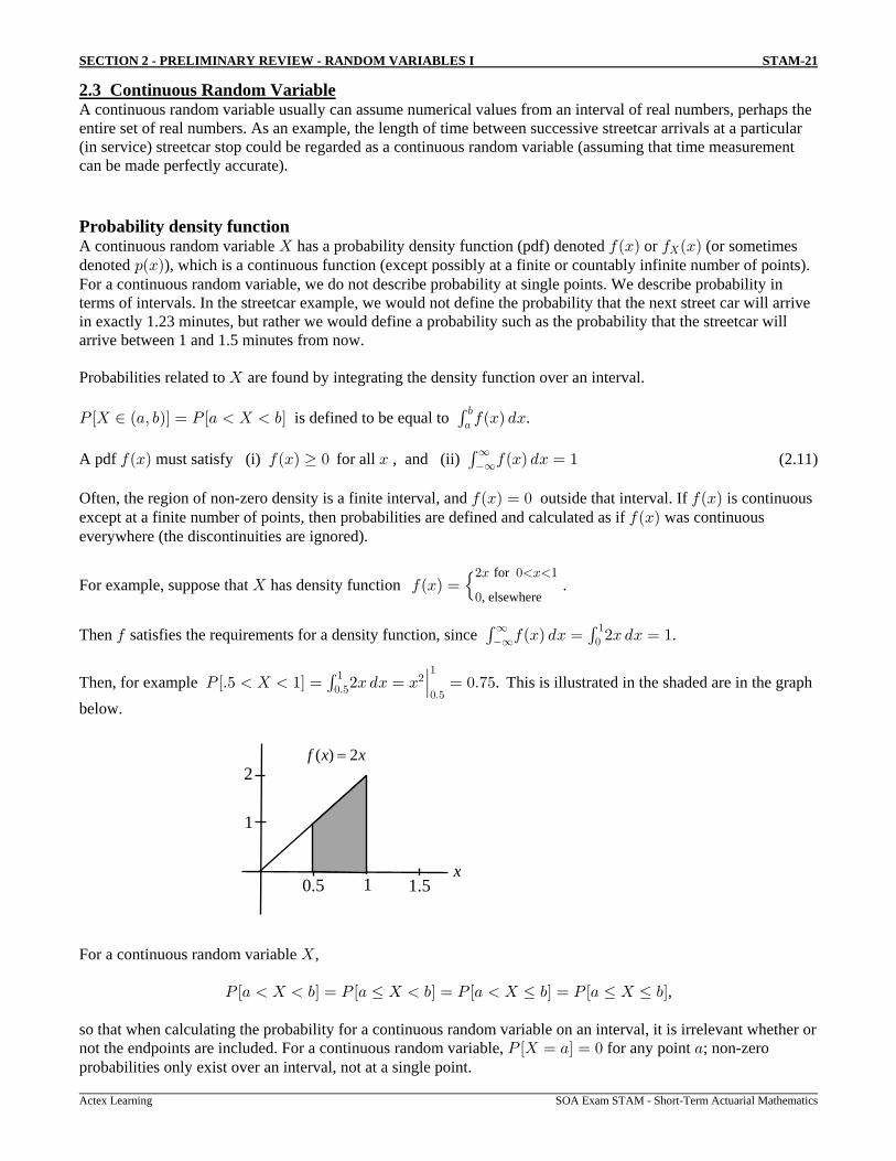
For example, suppose that has density function .\ 0ÐBÑ œ #B !B"
!
for
, elsewhere
Then satisfies the requirements for a density function, since .0 0ÐBÑ .B œ #B .B œ " ∞ !
∞ "
Then, for example . This is illustrated in the shaded are in the graphT ÒÞ& \ "Ó œ #B .B œ B œ !Þ(& !Þ&
" #
!Þ&
"
below.
2
1
( ) 2f x x
0.5 1x
1.5
For a continuous random variable ,\
TÒ+ \ ,Ó œ T Ò+ Ÿ \ ,Ó œ T Ò+ \ Ÿ ,Ó œ T Ò+ Ÿ \ Ÿ ,Ó,
so that when calculating the probability for a continuous random variable on an interval, it is irrelevant whether ornot the endpoints are included. For a continuous random variable, for any point ; non-zeroT Ò\ œ +Ó œ ! +probabilities only exist over an interval, not at a single point.
STAM-22 SECTION 2 - PRELIMINARY REVIEW - RANDOM VARIABLES I
Actex Learning SOA Exam STAM - Short-Term Actuarial Mathematics
2.4 Mixed DistributionA random variable may have some points with non-zero and with a continuous pdf elsewhere.probability massSuch a distribution may be referred to as a mixed distribution, but the general notion of mixtures of distributionswill be covered later. The sum of the probabilities at the discrete points of probability plus the integral of thedensity function on the continuous region for must be 1. For example, suppose that has probability of at\ \ !Þ&\ œ ! \ Ð!ß "Ñ 0ÐBÑ œ B, and is a continuous random variable on the interval with density function for! B " \, and has no density or probability elsewhere. This satisfies the requirements for a random variablesince the total probability is
T Ò\ œ !Ó 0ÐBÑ .B œ !Þ& B .B œ !Þ& !Þ& œ " ! !" " .
Then,T Ò! \ !Þ&Ó œ B .B œ !Þ"#&ß
!Þ&
andT Ò! Ÿ \ !Þ&Ó œ T Ò\ œ !Ó T Ò! \ !Þ&Ó œ !Þ& !Þ"#& œ !Þ'#&.
Notice that for this random variable because there is a probability mass atT Ò! \ !Þ&Ó Á T Ò! Ÿ \ !Þ&Ó\ œ !.
2.5 Cumulative Distribution Function, Survival Function and Hazard FunctionGiven a random variable , the cumulative distribution function of (also called the , or\ \ distribution functioncdf) is (also denoted ).JÐBÑ œ T Ò\ Ÿ BÓ J ÐBÑ\
The cdf is the "left-tail" probability, or the probability to the left of .JÐBÑ Band including
The survival function is the complement of the distribution function,
(2.12)WÐBÑ œ " JÐBÑ œ T Ò\ BÓ
The event is referred to as a "tail" or right tail of the distribution.\ B
For any cdf . (2.13)T Ò+ \ Ÿ ,Ó œ JÐ,Ñ JÐ+Ñß J ÐBÑ œ "ß J ÐBÑ œ !lim limBÄ∞ BÄ∞
For a discrete random variable with probability function , , and:ÐBÑ J ÐBÑ œ :ÐAÑAŸB
in this case is a "step function" (see Example 2-1 below); it has a jump (or step increase) at each point thatJÐBÑhas non-zero probability, while remaining constant until the next jump. Note that for a discrete random variable,JÐBÑ B B includes the probability at the point as well as the total probabilities of all the points to the left of .
If has a continuous distribution with density function , then\ 0ÐBÑ
and (2.14)JÐBÑ œ TÐ\ Ÿ BÑ œ 0Ð>Ñ .> WÐBÑ œ TÐ\ BÑ œ 0Ð>Ñ .> ∞ B
B ∞
and is a continuous, differentiable, non-decreasing function such thatJÐBÑ
..B J ÐBÑ œ J ÐBÑ œ W ÐBÑ œ 0ÐBÑw w .
Also, for a continuous random variable, the or ishazard rate failure rate
(2.15)2ÐBÑ œ œ œ 68WÐBÑ0 ÐBÑ 0 ÐBÑ
"JÐBÑ WÐBÑ .B.
If is continuous and , then the survival function satisfies and \ \ ! WÐ!Ñ œ " WÐBÑ œ / Þ 2Ð>Ñ .>!B
The iscumulative hazard function (2.16)LÐBÑ œ 2Ð>Ñ .>
!B
SECTION 2 - PRELIMINARY REVIEW - RANDOM VARIABLES I STAM-23
Actex Learning SOA Exam STAM - Short-Term Actuarial Mathematics
If has a mixed distribution with some discrete points and some continuous regions, then is continuous\ JÐBÑexcept at the points of non-zero probability mass, where will have a jump.JÐBÑ
The region of positive probability of a random variable is called the of the random variable.support
2.6 Examples of Distribution FunctionsThe following examples illustrate the variety of distribution functions that can arise from random variables. The supportof a random variable is the set of points over which there is positive probability or density.
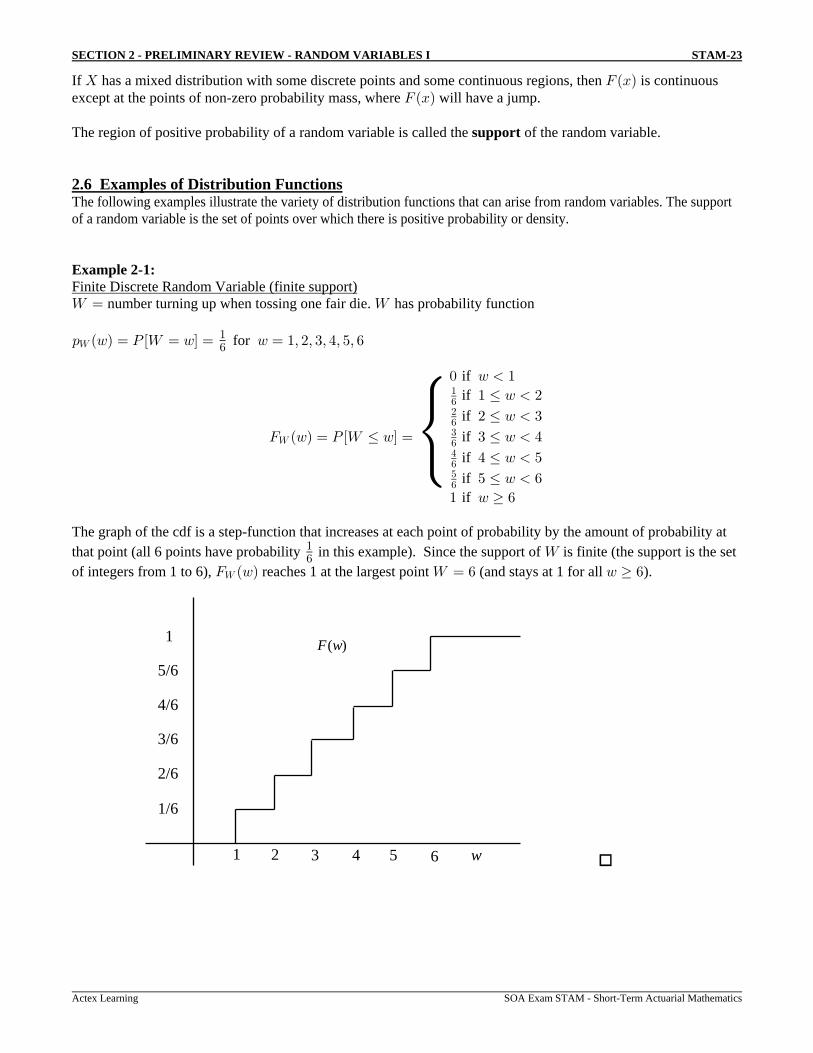
Example 2-1:Finite Discrete Random Variable (finite support)[ œ [number turning up when tossing one fair die. has probability function
: ÐAÑ œ T Ò[ œ AÓ œ A œ "ß #ß $ß %ß &ß '["' for
J ÐAÑ œ T Ò[ Ÿ AÓ œ
! A "
" Ÿ A #
# Ÿ A $
$ Ÿ A %
% Ÿ A &
& Ÿ A '
" A '
[
"'#'$'%'&'
if
if
if
if
if
if if
The graph of the cdf is a step-function that increases at each point of probability by the amount of probability atthat point (all 6 points have probability in this example). Since the support of is finite (the support is the set"
' [
of integers from 1 to 6), reaches 1 at the largest point (and stays at 1 for all ).J ÐAÑ [ œ ' A '[
1
5/6
4/6
3/6
2/6
1/6
1 2 3 4 5
( )F w
6 w
STAM-24 SECTION 2 - PRELIMINARY REVIEW - RANDOM VARIABLES I
Actex Learning SOA Exam STAM - Short-Term Actuarial Mathematics
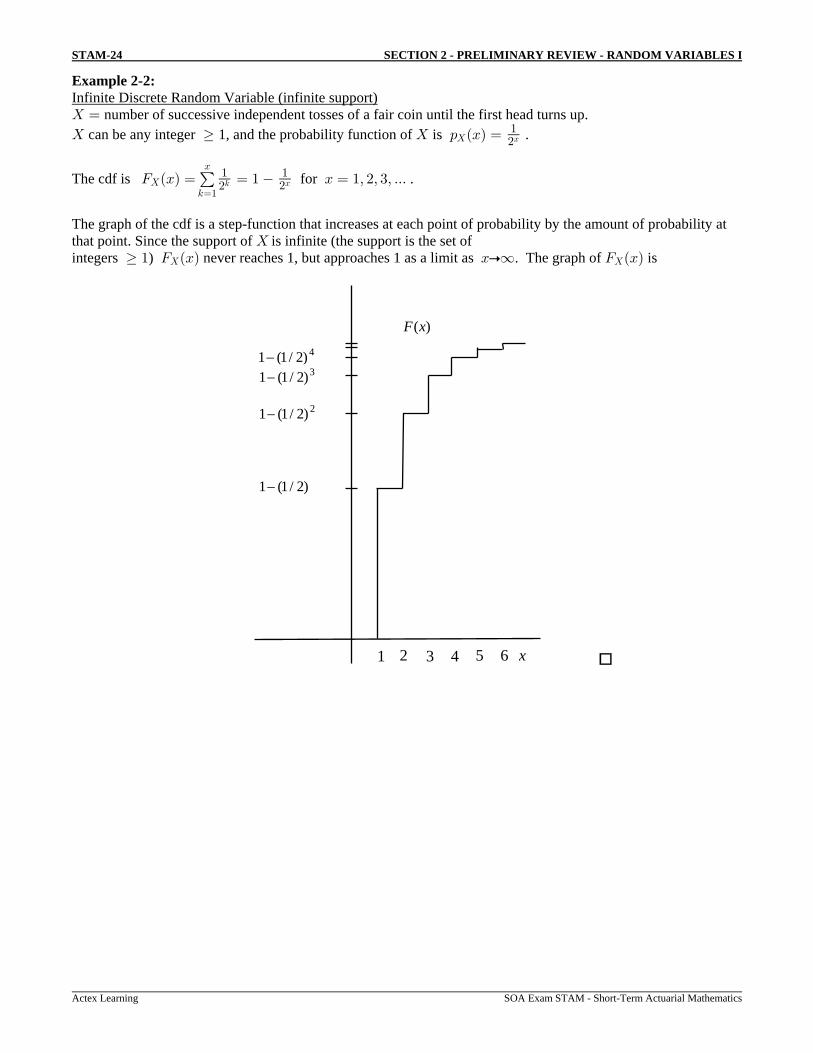
Example 2-2:Infinite Discrete Random Variable (infinite support)\ œ number of successive independent tosses of a fair coin until the first head turns up.\ \ : ÐBÑ œ can be any integer 1, and the probability function of is .\
"#B
The cdf is for .J ÐBÑ œ œ " B œ "ß #ß $ß ÞÞÞ\5œ"
B " "# #5 B
The graph of the cdf is a step-function that increases at each point of probability by the amount of probability atthat point. Since the support of is infinite (the support is the set of\integers ) never reaches 1, but approaches 1 as a limit as . The graph of is " J ÐBÑ Bp∞ J ÐBÑ\ \
( )F x
1 2 3 4 5 6 x
41 (1/ 2) 31 (1/ 2)
21 (1/ 2)
1 (1/ 2)
SECTION 2 - PRELIMINARY REVIEW - RANDOM VARIABLES I STAM-25
Actex Learning SOA Exam STAM - Short-Term Actuarial Mathematics
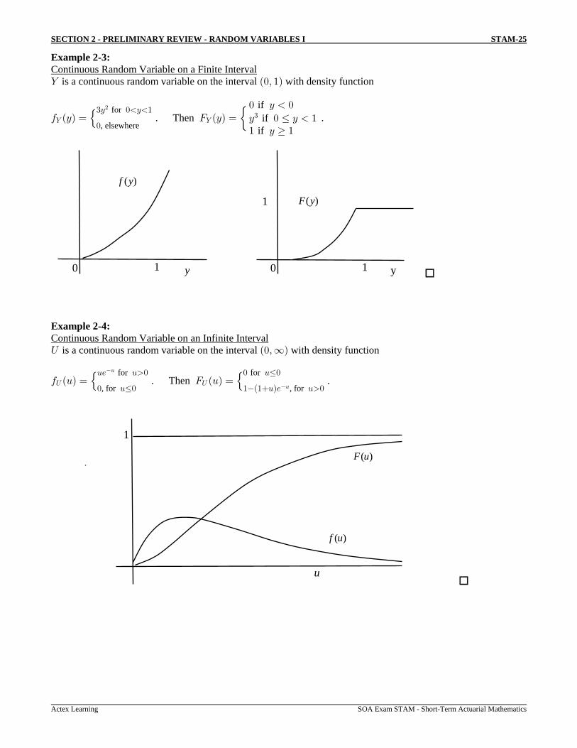
Example 2-3:Continuous Random Variable on a Finite Interval] Ð!ß "Ñ is a continuous random variable on the interval with density function
0 ÐCÑ œ J ÐCÑ œ
! C !
C ! Ÿ C "" C "
] ]$ $C !C"
!
# for
, elsewhere . Then .
if if
if
( )f y
y 1 0
( )F y
y10
1
Example 2-4:Continuous Random Variable on an Infinite IntervalY Ð!ß∞Ñ is a continuous random variable on the interval with density function
0 Ð?Ñ œ J Ð?Ñ œY Y ?/ ?! ! ?Ÿ!
! ?Ÿ! "Ð"?Ñ/ ?!
?
?
for for
, for , for . Then .
1
( )F u
( )f u
u
STAM-26 SECTION 2 - PRELIMINARY REVIEW - RANDOM VARIABLES I
Actex Learning SOA Exam STAM - Short-Term Actuarial Mathematics
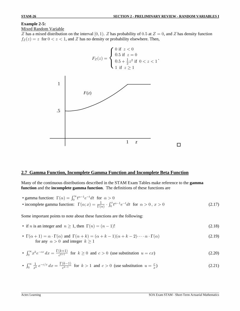
Example 2-5:Mixed Random Variable^ Ò!ß "Ñ ^ !Þ& ^ œ ! ^ has a mixed distribution on the interval . has probability of at , and has density function0 ÐDÑ œ D ! D " ^^ for , and has no density or probability elsewhere. Then,
if if
if
if
J ÐDÑ œ
! D !
Þ& D œ !
Þ& D ! D "
" D "
^ # !
! "#
.
1
.5
( )F z
1 z
2.7 Gamma Function, Incomplete Gamma Function and Incomplete Beta Function
Many of the continuous distributions described in the STAM Exam Tables make reference to the gammafunction incomplete gamma function and the . The definitions of these functions are
• gamma function: for > α αÐ Ñ œ > / .> !!
∞ " >α
• incomplete gamma function: for (2.17)> α αÐ à BÑ œ † > / .> ! ß B !"Ð Ñ> α
!B " >α
Some important points to note about these functions are the following:
• if is an integer and 1, then (2.18)8 8 Ð8Ñ œ Ð8 "Ñx>
• and (2.19)> α α > α > α α α α > αÐ "Ñ œ † Ð Ñ Ð 5Ñ œ Ð 5 "ÑÐ 5 #Ñâ † † Ð Ñ for any and integer α ! 5 "
• for and (use substitution ) (2.20)!
∞ 5 -BB / .B œ 5 ! - ! ? œ -B>Ð5"Ñ-5"
• for and (use substitution ) (2.21)!
∞ -ÎB" -B -
Ð5"ÑB5 5"/ .B œ 5 " - ! ? œ
>
SECTION 2 - PRELIMINARY REVIEW - RANDOM VARIABLES I STAM-27
Actex Learning SOA Exam STAM - Short-Term Actuarial Mathematics
Some of the table distributions make reference to the , which is defined as follows:incomplete beta function
for , (2.22)"Ð+ß ,à BÑ œ > Ð" >Ñ .> ! Ÿ B Ÿ " +ß , !>> >
Ð+,ÑÐ+Ñ Ð,Ñ
!B +" ,"
References to the gamma function have been rare and the incomplete functions have not been referred to on the
released exams. It is useful to remember the integral relationship !∞ 5 -BB / .B œ>Ð5"Ñ-5" , particularly in the case
in which is a non-negative integer.5
In that case, we get , which can occasionally simplify integral relationships. This!
∞ 5 -BB / .B œ 5x-5"
relationship is embedded in the definition of the gamma distribution in the STAM Exam Table.
The pdf of the gamma distribution with parameters and is , defined on the interval .α ) 0Ð>Ñ œ > !> /Ð Ñ
α )
α
" >Î
) > α
This means that , which can be reformulated as If we let ! !∞ ∞ " >Î> /
Ð Ñ
α )
α
" >Î
) > α .> œ " > / .B œ Ð ÑÞα ) α) > α
) αœ 5 œ ""- and , we get the relationship
(2.23)!
∞ 5 -BB / .B œ>Ð5"Ñ-5"
Looking at the various continuous distributions in the STAM Exam Table gives some hints at calculating anumber of integral forms. For instance, the pdf of the beta distribution with parameters is+ß ,ß œ ")
0ÐBÑ œ ‚ B Ð" BÑ ! B ">> >
Ð+,ÑÐ+Ñ Ð,Ñ
+" ," for .
Therefore, , from which we get!
" +" ,>> >
Ð+,ÑÐ+Ñ Ð,Ñ ‚ B Ð" BÑ .B œ "
!
" +" ,"B Ð" BÑ .B œ> >>Ð+Ñ Ð,ÑÐ+,Ñ .

STAM-28 SECTION 2 - PRELIMINARY REVIEW - RANDOM VARIABLES I
Actex Learning SOA Exam STAM - Short-Term Actuarial Mathematics
SECTION 2 PROBLEM SET STAM-29
Actex Learning SOA Exam STAM - Short-Term Actuarial Mathematics
SECTION 2 PROBLEM SETPreliminary Review - Random Variables I
1. Let be a discrete random variable with probability function\
for What is the probability that is even?T Ò\ œ BÓ œ B œ "ß #ß $ß ÞÞÞ \#$B
A) B) C) D) E)" # " # $% ( $ $ %
2. For a certain discrete random variable on the non-negative integers, the probability function satisfies therelationships
and for Find .TÐ!Ñ œ TÐ"Ñ T Ð5 "Ñ œ † T Ð5Ñ 5 œ "ß #ß $ß ÞÞÞ T Ð!Ñ"5
A) B) C) D) E) 68 / / " Ð/ "Ñ / Ð/ "Ñ" " "
3. Let be a continuous random variable with density function\
. Calculate .0ÐBÑ œ T Ò l\ l Ó 'BÐ"BÑ !B"
!
" "# %
for
otherwise A) B) C) D) E) !Þ!&#" !Þ"&'$ !Þ$"#& !Þ&!!! !Þ)!!!
4. Let be a random variable with distribution function\
. Calculate .
for for
for
for for
JÐBÑ œ T Ò" Ÿ \ Ÿ #Ó
! B !! Ÿ B "
" Ÿ B #
# Ÿ B $
" B $
B)" B% )$ B% "#
A) B) C) D) E) " $ ( "$ "*) ) "' #% #%
5. Let and be three independent continuous random variables each with density function\ ß \ \" # $
0ÐBÑ œ #B !B #
!
for
otherwise .
What is the probability that exactly 2 of the 3 random variables exceeds 1?
A) B) C) $# # $ # # $Ð # "ÑÐ# #Ñ #
D) E) Ð #Ñ Ð # Ñ $Ð #Ñ Ð # Ñ$ " $ "# # # #
# #
6. Let and be three independent, identically distributed random variables each with density\ ß \ \" # $
function . Let . Find .0ÐBÑ œ ] œ 7+BÖ\ ß\ ß\ × T Ò] Ó $B !ŸBŸ"
!
"#
# for
otherwise" # $
A) B) C) D) E) " $( $%$ ( &""'% '% &"# ) &"#
7. Let the distribution function of for be .\ B ! JÐBÑ œ " 5œ!
$B /5x
5 B
What is the density function of for ?\ B !
A) B) C) D) E)/ / /B B B B / B / B / B /# ' ' '
# B $ B $ B $ B
STAM-30 SECTION 2 PROBLEM SET
Actex Learning SOA Exam STAM - Short-Term Actuarial Mathematics
8. Let have the density function for , and , otherwise.\ 0ÐBÑ œ ! B 0ÐBÑ œ !$B#
$) )
If , find the value of .T Ò\ "Ó œ () )
A) B) C) D) E) " ( )# ) (
"Î$ "Î$ "Î$Ð Ñ Ð Ñ # #
9. A large wooden floor is laid with strips 2 inches wide and with negligible space between strips. A uniformcircular disk of diameter 2.25 inches is dropped at random on the floor. What is the probability that the disktouches three of the wooden strips?
A) B) C) D) E) " " " " "% )1 1 1 #
10. If has a continuous uniform distribution on the interval from 0 to 10, then what is ?\ TÒ\ (Ó"!\
A) B) C) D) E) $ $" " $* ("! (! # (! "!
11. For a loss distribution where , you are given:B #
i) The hazard rate function: , for 2ÐBÑ œ B #D#B
#
ii) A value of the distribution function: JÐ&Ñ œ !Þ)% Calculate .D A) 2 B) 3 C) 4 D) 5 E) 6
SECTION 2 PROBLEM SET STAM-31
Actex Learning SOA Exam STAM - Short-Term Actuarial Mathematics
SECTION 2 PROBLEM SET SOLUTIONS
1. is even . T Ò\ Ó œ T Ò\ œ #Ó T Ò\ œ %Ó T Ò\ œ 'Ó â œ † Ò âÓ œ † œ# " " " # " "$ $ $ $ $ %"$ & # "
$#
Answer: A
2. , . . . .TÐ#Ñ œ TÐ"Ñ œ TÐ!Ñ ß T Ð$Ñ œ † T Ð#Ñ œ † T Ð!Ñ T Ð5Ñ œ † T Ð!Ñ" " "# #x Ð5"Ñx
The probability function must satisfy the requirement so that3œ!
∞
TÐ3Ñ œ "
TÐ!Ñ † T Ð!Ñ œ TÐ!ÑÐ" /Ñ œ "3œ"
∞"
Ð3"Ñx
(this uses the series expansion for at ). Then, . Answer: C/ B œ " TÐ!Ñ œB "/"
3. T Ò \ Ÿ Ó œ T Ò Ÿ \ Ÿ Ó œ T Ò Ÿ \ Ÿ Ó œ 'BÐ" BÑ .B " " " " " " $# % % # % % % "Î%
$Î%
. Answer: Cœ Þ')(& p T Ò \ Ó œ " T Ò \ Ó œ !Þ$"#& " " " "# % # %
4. Answer: ET Ò" Ÿ \ Ÿ #Ó œ T Ò\ Ÿ #Ó T Ò\ "Ó œ JÐ#Ñ JÐBÑ œ œ ÞlimBÄ"
"" " "*"# ) #%
5. .T Ò\ Ÿ "Ó œ Ð # BÑ .B œ # ß T Ò\ "Ó œ " T Ò\ Ÿ "Ó œ # !
" " $# #
With 3 independent random variables, and , there are 3 ways in which exactly 2 of the 's\ ß \ \ \" # $ 3
exceed 1 (either or or ).\ ß\ \ ß\ \ ß\" # " $ # $
Each way has probability ÐT Ò\ "ÓÑ † T Ò\ Ÿ "Ó œ Ð #Ñ Ð # Ñ# #$ "# #
for a total probability of . Answer: E$ † Ð #Ñ Ð # Ñ$ "
# # #
6. T Ò] Ó œ " T Ò] Ÿ Ó œ " T ÒÐ\ Ÿ Ñ ∩ Ð\ Ÿ Ñ ∩ Ð\ Ÿ ÑÓ" " " " "# # # # #" # $
Answer: Eœ " ÐT Ò\ Ÿ ÓÑ œ " Ò $B .BÓ œ " Ð Ñ œ Þ" " &""# ) &"#
$ # $ $!"Î#
7. 0ÐBÑ œ J ÐBÑ œ œ / †w B
5œ! 5œ!
$ $ 5B / B / B 5B5x 5x
5" B 5 B 5 5"
Answer: Cœ / † Ò" Ó œ ÞB B" B #B B $B / B" # ' '
# $ # B $
8. Since if , and since , we must conclude that .0ÐBÑ œ ! B T Ò\ "Ó œ ") )()
Then, , or equivalently, . Answer: ET Ò\ "Ó œ 0ÐBÑ .B œ .B œ " œ œ # " ") ) $B " (
)
#
$ $) ) )
STAM-32 SECTION 2 PROBLEM SET
Actex Learning SOA Exam STAM - Short-Term Actuarial Mathematics
9. Let us focus on the left-most point on the disk. Consider two adjacent strips on the floor. Let the interval:Ò!ß #Ó : ! "Þ(& represent the distance as we move across the left strip from left to right. If is between and ,then the disk lies within the two strips.
If is between and , the disk will lie on 3 strips (the first two and the next one to the right). Since: "Þ(& #any point between and is equally likely as the left most point on the disk (i.e. uniformly distributed! # :
between and ) it follows that the probability that the disk will touch three strips is .! # œ !Þ#& "# )
Answer: D
10. Since the density function for is for , we can regard as being positive. Then\ 0ÐBÑ œ ! B "! \""!
T Ò\ (Ó œ T Ò\ (\ "! !Ó œ T ÒÐ\ &ÑÐ\ #Ñ !Ó"!\
#
œ TÒ\ &Ó T Ò\ #Ó
(since if either both Ð> &ÑÐ> #Ñ ! > &ß > # !
or both ) . Answer: E> &ß > # ! œ œ& # ("! "! "!
11. The survival function for a random variable can be formulated in terms of the hazard rate function:WÐCÑWÐCÑ œ /B:Ò 2ÐBÑ .BÓ
∞
C .
In this question, .WÐ&Ñ œ " JÐ&Ñ œ !Þ"' œ /B:Ò .BÓ œ /B:Ò 68Ð ÑÓ#
& D D &#B # #
# #
Taking natural log of both sides of the equation results in , and solving for 68Ð Ñ œ 68Ð!Þ"'Ñ DD &# #
#
results in . Answer: AD œ #
SECTION 3 - PRELIMINARY REVIEW - RANDOM VARIABLES II STAM-33
Actex Learning SOA Exam STAM - Short-Term Actuarial Mathematics
SECTION 3 - PRELIMINARY REVIEW - RANDOM VARIABLES II
This section relates to Sections 3.1 - 3.3 of "Loss Models". The mean and variance of a random variable are twofundamental distribution parameters. In this section we review those and some other important distribution parameters.Chapter 3 of Loss models also introduces deductibles and policy limits. These topics will be considered in detail later inthe study guide.
The suggested time frame for this section is 2 hours.
3.1 Expected Value and Other Moments of a Random VariableFor a random variable , the expected value is denoted , or or . The expected value of is also\ IÒ\Ó \. .\
called the , or the . The expected value is the "average" over the range of values thatexpectation of mean of \ \\ can be, or the "center" of the distribution.
For a discrete random variable, the expected value of is (3.1)\ all B
B ‚ :ÐBÑ
where the sum is taken over all points at which has non-zero probability. For instance, if is the result ofB \ \
one toss of a fair die, then IÒ\Ó œ " ‚ # ‚ â ' ‚ œ Þ" " " (' ' ' #
For a continuous random variable, the expected value is
∞
∞B 0ÐBÑ .B‚ (3.2)
Although the integral is written with lower limit and upper limit , the interval of integration is the interval∞ ∞of support (non-zero-density) for . For instance, if for , then the mean is\ 0ÐBÑ œ #B ! B "
IÒ\Ó œ B ‚ #B .B œ!
" #$ .
If is a function, then is equal to if is a discrete random variable, and it is equal to2 IÒ2Ð\ÑÓ 2ÐBÑ ‚ :ÐBÑ \B
∞
∞2ÐBÑ ‚ 0ÐBÑ .B \ IÒ2Ð\ÑÓ 2Ð\Ñ if is a continuous random variable. is the "average" value of based on the
possible outcomes of random variable .\
The mean of a random variable might not exist\ , it might be or . For example, the continuous∞ ∞random variable with\
pdf has expected value .0ÐBÑ œ B ‚ .B œ ∞ "B#
#
for
, otherwise
B "
!
"B "
∞
For any constants and and functions and ,+ ß + , 2 2" # " #
(3.3)IÒ+ 2 Ð\Ñ + 2 Ð\Ñ ,Ó œ + IÒ2 Ð\ÑÓ + IÒ2 Ð\ÑÓ ," " # # " " # #
If is a non-negative random variable (defined on or ) then \ Ò!ß∞Ñ Ð!ß∞Ñ
IÒ\Ó œ Ò" JÐBÑÓ . œ WÐBÑ . ! !
∞ ∞B B (3.4)
This relationship is valid for any random variable, discrete, continuous or with a mixeddistribution. Using the example on the previous page, thenif for , 0ÐBÑ œ #B ! B "
JÐBÑ œ ß Ò" JÐBÑÓ .B œ Ò" B Ó .B œ œ IÒ\Ó B !BŸ"
" B"
#$
# for
, for and . ! !
∞ " #
It tends to be more awkward to apply this rule to discrete random variables.
Jensen's Inequality states that if is a function such the on the probability space for , then1 1 ÐBÑ ! \ww
IÒ1Ð\ÑÓ 1ÐIÒ\ÓÑ IÒ\ Ó ÐIÒ\ÓÑ. For example, .# #
STAM-34 SECTION 3 - PRELIMINARY REVIEW - RANDOM VARIABLES II
Actex Learning SOA Exam STAM - Short-Term Actuarial Mathematics
Moments of a random variableIf is an integer, then the is (sometimes denoted ) and is8 " IÒ\ Ó8 \th (raw) moment of 8 w
8.
in the discrete case, and in the continuous case. (3.5) all B
8 8∞∞
B ‚ :ÐBÑ B ‚ 0ÐBÑ .B
If the mean of is , then the is defined to be \ IÒÐ\ Ñ Ó. .8 \th central moment of (about the mean ). 8
and may be denoted ..8
For instance, the 3rd central moment of the fair die toss random variable is\
IÒÐ\ Ñ Ó œ Ð" Ñ ‚ Ð# Ñ ‚ â Ð' Ñ ‚ œ !( ( " ( " ( "# # ' # ' # '
$ $ $ $ .
The 2nd central moment of the continuous random variable pdf\ 0ÐBÑ œ #B ! B " for is!" #ÐB Ñ #B .B œ#
$ ‚ "") .
Variance of \The variance of is denoted , , or . It is defined to be equal to\ Z +<Ò\Ó Z Ò\Ó 5 5# #
\
Z +<Ò\Ó œ IÒÐ\ Ñ Ó œ IÒ\ Ó œ IÒ\ Ó ÐIÒ\ÓÑ. .\# # # # #
\ (3.6)
The representation of as is often the most convenient one to use. The variance is theZ +<Ò\Ó IÒ\ Ó ÐIÒ\ÓÑ# #
2nd central moment of ; .\ œ Z +<Ò\Ó œ . . .# #w #
Variance is a measure of the "dispersion" of about the mean. Being the expected value of , the\ Ð\ Ñ.\#
variance is the average squared deviation of from its mean .\ .\
A large variance indicates significant levels of probability or density for points far from . The variance is alwaysIÒ\Ó ! \ ! \ " (the variance of is equal to only if has a discrete distribution with a single point and probability at that
point; in other words, not random at all).
The random variable has mean and variance .prob. .5prob. .5
Y œ IÒY Ó œ & Z +<ÒY Ó œ "%'
The random variable has the same mean as , , but has variance .
prob. .5prob. .5
[ œ Y IÒ[ Ó œ & Z +<Ò[ Ó œ *#)
The higher variance of is indicative of the further dispersion of the outcomes of from the mean 5 as[ [compared to .Y
If and are constants, then .+ , Z +<Ò+\ ,Ó œ + Z +<Ò\Ó#
Here is a useful shortcut for finding the variance of a 2-point discrete random variable.
If is the two-point random variable Prob. Prob.
\ \ œ+ :, " :
then .Z +<Ò\Ó œ Ð, +Ñ ‚ : ‚ Ð" :Ñ# (3.7)
Standard deviation of \The standard deviation of the random variable is the square root of the variance, and is denoted\
5\ œ Z +<Ò\Ó .

SECTION 3 - PRELIMINARY REVIEW - RANDOM VARIABLES II STAM-35
Actex Learning SOA Exam STAM - Short-Term Actuarial Mathematics
Coefficient of variationThe coefficient of variation of is\
5.\
\œ
Z +<Ò\Ó
IÒ\Ó . (3.8)
Skewness and kurtosis
The skewness of is , and the kurtosis is (3.9)\ IÒÐ\ Ñ Ó IÒÐ\ Ñ Ó. .5 5
$ %
$ %
Skewness measures the symmetry of a random variable; skewness of 0 indicates a distribution which is symmetricaround its mean. The fair dies toss random variable has skewness of 0. Kurtosis is a measure of the "peakedness"of a distribution. Higher kurtosis suggests that more of the variance is due to less frequent large deviations, ratherthan more frequent smaller deviations.There have been infrequent references to skewness and kurtosis on the STAM Exam.
3.2 Moment generating function of random variable \The moment generating function of (mgf) is denoted or , and it is defined to be\ Q Ð>Ñ ß 7 Ð>Ñ ß QÐ>Ñ 7Ð>Ñ\ \
Q Ð>Ñ œ IÒ/ Ó\>\ , which is either
B
>B >B∞
∞/ :ÐBÑ / 0ÐBÑ .B if is discrete, or if is continuous (3.10)\ \
It is always true that .Q Ð!Ñ œ "\
The moment generating function of might not exist for all real numbers, but usually exists on some interval of\real numbers. The function is called the . The function 68ÒQ Ð>ÑÓ Q Ð68\ \cumulant generating function>Ñ œ IÒ> Ó\ is called the and may be denoted ; the probabilityprobability generating function T Ð>Ñ œ IÒ> Ó\
\
generating function is usually used in the case of a discrete random variable.
Some properties of moment and probability generating functionsSuppose that for the random variable , the moment generating function exists in an interval\ Q Ð>Ñ\
containing the point . Then> œ !
..>
8
8 Q Ð>Ñ œ Q Ð!Ñ œ IÒ\ Ó œ\>œ!
Ð8Ñ\
8 w8 . , the -th moment of , and (3.11)8 \
. ..> Q Ð!Ñ .>
Q Ð!Ñ68ÒQ Ð>ÑÓ œ œ IÒ\Ó 68ÒQ Ð>ÑÓ œ Z +<Ò\Ó\ \
>œ! >œ! \
w
\
#
#, and (3.12)
If and are random variables, and for all values of in an interval containing ,\ \ Q Ð>Ñ œ Q Ð>Ñ > > œ !" # \ \" #
then and have identical probability distributions.\ \" #
If are independent random variables and then\ ß\ ß ÞÞÞß \ W œ \" # 8 33œ"
8 (3.13)Q Ð>Ñ œ Q Ð>Ñ ‚Q Ð>Ñ ‚ † † † ‚Q Ð>Ñ œ Q Ð>ÑW \ \ \ \
3œ"
8
" # 8 3
If has a discrete non-negative integer distribution with , then the probability generating\ : œ T Ò\ œ 5Ó5
function is
(3.14)T Ð>Ñ œ : : ‚ > : ‚ > â œ : ‚ >\ ! " # 5# 5
5œ!
∞and .T Ð!Ñ œ :\ !
STAM-36 SECTION 3 - PRELIMINARY REVIEW - RANDOM VARIABLES II
Actex Learning SOA Exam STAM - Short-Term Actuarial Mathematics
3.3 Percentiles and Quantiles of a distributionIf , then the -th percentile of the distribution of is the number which satisfies the following! : " "!!: \ -:inequalities: J Ò- Ó œ T Ò\ - Ó Ÿ : Ÿ T Ò\ Ÿ - Ó œ J Ò- Ó:
: : : . (3.15)
For a continuous random variable, it is sufficient to find the for which . If , - T Ò\ Ÿ - Ó œ : : œ Þ&: : the 50-thpercentile of a distribution is referred to as the median of the distribution, it is the point for whichQTÒ\ Ÿ QÓ œ Þ& Q Q. The median is the 50% probability point, half of the distribution probability is to the left of andhalf is to the right. The word "quantile" is a general term for the proportion or percent of a distribution below a certaingiven point and is often used interchangeably with "percentile".
3.4 The mode of a distributionThe mode is any point at which the probability or density function is maximized. For the fair die toss7 0ÐBÑrandom variable, each of or would satisfy the requirements of being a mode, since theB œ "ß #ß $ß %ß & 'probability at each point is , which is the maximum probability of any individual point. For the continuous"
'
random variable with for , strictly speaking, there is no mode since the upper bound of the0ÐBÑ œ #B ! B "density of 2 is never reached. The mode could be described as occurring at 1 as a limit.
Example 3-1:Let equal the number of tosses of a fair die until the first "1" appears. Find .\ IÒ\ÓSolution:\ " is a discrete random variable that can take on any integer value . The probability that the first 1 appears on
the -th toss is for ( tosses that are not , followed by a 1). This is theB 0ÐBÑ œ B " B " "Ð Ñ Ð Ñ& "' '
B"
probability function of . Then\
IÒ\Ó œ 5 ‚ 0Ð5Ñ œ 5 ‚ œ Ò" # $ âÓ 5œ" 5œ"
∞ ∞5" #Ð Ñ Ð Ñ Ð Ñ Ð Ñ Ð Ñ& " " & &
' ' ' ' ' .
We use the general increasing geometric series relation ," #< $< â œ# "Ð"<Ñ#
so that . IÒ\Ó œ ‚ œ 'Ð Ñ" "' Ð" Ñ&'
#
Example 3-2:
The moment generating function of is for , where .\ > ! αα> α α
Find .Z +<Ò\ÓSolution:
Z +<Ò\Ó œ IÒ\ Ó ÐIÒ\ÓÑ IÒ\Ó œ Q Ð!Ñ œ# # w\. α
αÐ >Ñ# >œ!
œ "α ,
and .IÒ\ Ó œ œ p Z +<Ò\Ó œ œ# #
>œ!Q Ð!Ñ œww
\#
Ð >Ñα
α $ # # " "α α α α# # #Ð Ñ
Alternatively, 68Q Ð>Ñ œ 68 œ 68 68Ð >Ñ p\ Ð Ñαα α> .> >
. "α α 68ÒQ Ð>ÑÓ œ\
and so that . " . ".> Ð >Ñ .>
# #
# # # #68ÒQ Ð>ÑÓ œ Z +<Ò\Ó œ 68ÒQ Ð>ÑÓ œ Þ\ \>œ!α α
SECTION 3 - PRELIMINARY REVIEW - RANDOM VARIABLES II STAM-37
Actex Learning SOA Exam STAM - Short-Term Actuarial Mathematics
Example 3-3:Given that the density function of is , for , and elsewhere, find the -th moment of ,\ 0ÐBÑ œ / B ! ! 8 \) B)
where is a non-negative integer (assuming that ).8 !)Solution:The -th moment of is . Applying integration by parts, this can be written as8 \ IÒ\ Ó œ B † / .B8 8 B
!∞ ) )
! ! !∞ ∞ ∞8 B 8 B 8" B 8" B
Bœ!
Bϰ
B .Ð / Ñ œ B / 8B / .B œ 8B / .BÞ) ) ) )
Repeatedly applying integration by parts results in . It is worthwhile noting the general form of theIÒ\ Ó œ8 8x)8
integral that appears in this example; if is an integer and , then by repeated applications of5 ! + !
integration by parts, we have , so that in this example!∞ 5 +>> / .> œ 5x
+5"
! !∞ ∞8 B 8 BB / .B œ B / .B œ † œ) ) )) ) 8x 8x
) )8" 8 .
An alternative solution uses the moment generating functionÞ
Q Ð>Ñ œ IÒ/ Ó œ / / .B œ / .B œ\>\ >B B Ð >ÑB
! !
∞ ∞ ) )) ) ))>
(which will be valid for ). Then> )
Q Ð>Ñ œ IÒ\Ó œ Q Ð!Ñ œ Q Ð>Ñ œ IÒ\ Ó œ Q Ð!Ñ œ\ \w w #
\ \Ð#Ñ Ð#Ñ) )
) ) ) )Ð >Ñ Ð >Ñ" # #
# $ # so that , and so that .
It can be shown by induction on that so that . 8 Q Ð>Ñ œ IÒ\ Ó œ Q Ð!Ñ œ\ \Ð8Ñ Ð8Ñ88x 8x
Ð >Ñ)
) )8" 8
Example 3-4:The continuous random variable has pdf for .\ 0ÐBÑ œ / ∞ B ∞"
#lBl
Find the 87.5-th percentile of the distribution.Solution:The 87.5-th percentile is the number for which ., !Þ)(& œ T Ò\ Ÿ ,Ó œ 0ÐBÑ .B œ / .B
∞ ∞
, , lBl"#
Note that this distribution is symmetric about , since , so the mean and median are! 0Ð BÑ œ 0ÐBÑboth . Thus, , and so! , !
∞ ∞ ! !
lBl lBl lBl B! , ,, " " " "# # # #/ .B œ / .B / .B œ !Þ& / .B
œ !Þ& Ð" / Ñ œ !Þ)(& p , œ 68Ð!Þ#&Ñ œ 68 %"#
, .
Example 3-5:\ \ is the outcome after 1 toss of a fair die. Find the 25-th percentile of .Solution:The distribution function of was found earlier in Example 2-1 above. We see that\
JÐ# Ñ œ T Ò\ #Ó œ Ÿ !Þ#& Ÿ œ T Ò\ Ÿ #Ó œ JÐ#Ñ " #' ' . Any number other than 2 will not satisfy one side of
the inequalities. The 25-th percentile is 2. Note that 2 would also be the 20-th and the 30-th percentile; 2 wouldbe any percentile from 16.7-th to 33.3-rd.
STAM-38 SECTION 3 - PRELIMINARY REVIEW - RANDOM VARIABLES II
Actex Learning SOA Exam STAM - Short-Term Actuarial Mathematics
3.5 Random Samples And The Sampling Distribution
Suppose that is a random variable, say the outcome of a toss of a six-sided die. A \ random sample of size Rfrom the distribution of the random variable is a collection of independent observations from the distribution of\\ \ ß\ ß ÞÞÞß \, say . We can interpret the sample in two ways:" # R
(i) it is a collection of numerical values, the actual outcomes of successive tosses of the die, andR(ii) it is a collection of independent random variables; we don't know the actual die toss outcomes yetR
because the die hasn't been tossed, but there will be the outcomes after the die is tossedR \ ß\ ß ÞÞÞß \" # R
R times.
Each interpretation is useful depending upon the way in which the random sample is being used.
The random variable will have the usual associated parameters, such as the mean, and variance,\ IÒ\Ó œ .\
Z +<Ò\Ó œ 5\# , etc. Two of the main objectives in statistical estimation are finding estimates of quantities related
to , and determining some of the properties of those estimates.\
The simplest example of an is the of the random sample. It is the most commonly usedestimator sample meanestimator of the distribution mean , and is defined as follows:IÒ\Ó œ .\
(just the average of the sample). (3.16)\ œ œ \ \ \ â\
R R"" # R
3œ"
R
3
Under the two interpretations of random sample mentioned above, the sample mean is either\
(i) a number (representing an estimate of the mean of the distribution of ), or\(ii) a random variable (if each of the 's are interpreted as random variables).\3
Under interpretation (ii), in which the sample mean is a random variable, has a distribution referred to\ \
as the . Using basic rules of probability we can find the mean and variance of :_
sampling distribution \
IÒ\Ó œ I œ † ÐIÒ\ Ó IÒ\ Ó âIÒ\ ÓÑ Ò Ó\ \ â\
R R"" # R
" # R
. (3.17)œ † Ð â Ñ œ † ÐR † Ñ œ" "R R. . . . .\ \ \ \ \
Since the expected value of is , we say that is a random variable, and\ \
.\ \ is an unbiased estimate of ..\
has a variance.
Z +<Ò\Ó œ Z +< œ † ÐZ +<Ò\ Ó â Z +<Ò\ ÓÑ Ò Ó\ \ â\
R R"" # R# " R
. (3.18)œ † Ð â Ñ œ † ÐR † Ñ œ" "R R R# #
\#
5 5 5 5\ \ \ \# # # # 5
The third equality for the variance of follows from the assumption of independence of the 's.\ \
3
Keep in mind that we are describing properties of the sample mean .\
Another important estimator associated with a random sample of observations from the random variable is the\sample variance not to be confused with (unbiased form). The sample variance of the random sample ( Z +<Ò\Ó
ßwhich is the variance of the sample mean) is an estimator of , the variance of . It is definedZ +<Ò\Ó œ \5#\
as follows:
(also denoted or ) . (3.19)= œ Z +<Ò\Ó œ Ð\ \Ñs# #
\3œ"
R
3"
R" = s#
\#5
=# #\ \ is an unbiased estimate of .5
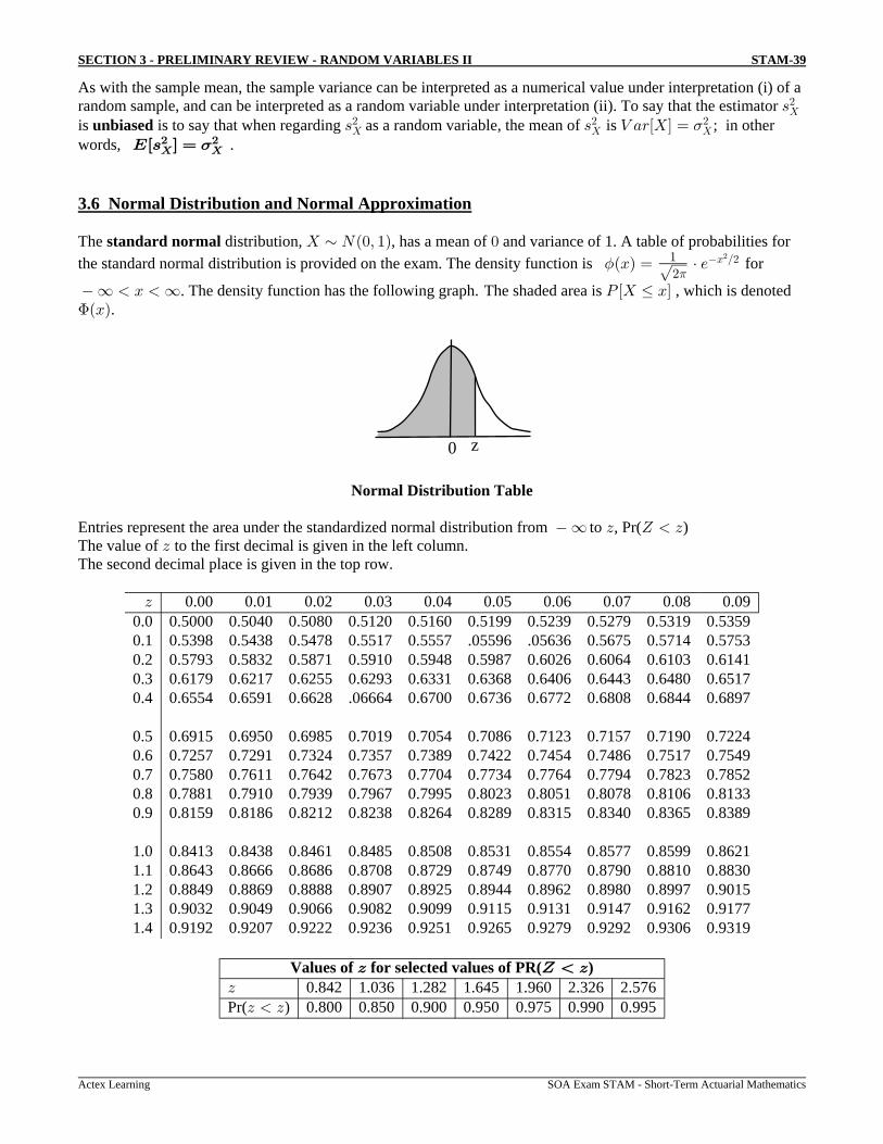
SECTION 3 - PRELIMINARY REVIEW - RANDOM VARIABLES II STAM-39
Actex Learning SOA Exam STAM - Short-Term Actuarial Mathematics
As with the sample mean, the sample variance can be interpreted as a numerical value under interpretation (i) of arandom sample, and can be interpreted as a random variable under interpretation (ii). To say that the estimator =#\is is to say that when regarding as a random variable, the mean of is ; in otherunbiased = = Z +<Ò\Ó œ# # #
\ \ \5words, .IÒ= Ó œ# #
\ \5
3.6 Normal Distribution and Normal Approximation
The distribution, , has a mean of and variance of 1. A table of probabilities forstandard normal \ µ RÐ!ß "Ñ !
the standard normal distribution is provided on the exam. The density function is 9ÐBÑ œ † /"
# 1B Î##
for
∞ B ∞. The density function has the following graph. The shaded area is , which is denotedT Ò\ Ÿ BÓFÐBÑ.
z0
Normal Distribution Table
Entries represent the area under the standardized normal distribution from to , Pr( )∞ D ^ DThe value of to the first decimal is given in the left column.DThe second decimal place is given in the top row.
D 0.00 0.01 0.02 0.03 0.04 0.05 0.06 0.07 0.08 0.090.0 0.5000 0.5040 0.5080 0.5120 0.5160 0.5199 0.5239 0.5279 0.5319 0.53590.1 0.5398 0.5438 0.5478 0.5517 0.5557 .05596 .05636 0.5675 0.5714 0.57530.2 0.5793 0.5832 0.5871 0.5910 0.5948 0.5987 0.6026 0.6064 0.6103 0.61410.3 0.6179 0.6217 0.6255 0.6293 0.6331 0.6368 0.6406 0.6443 0.6480 0.65170.4 0.6554 0.6591 0.6628 .06664 0.6700 0.6736 0.6772 0.6808 0.6844 0.6897
0.5 0.6915 0.6950 0.6985 0.7019 0.7054 0.7086 0.7123 0.7157 0.7190 0.72240.6 0.7257 0.7291 0.7324 0.7357 0.7389 0.7422 0.7454 0.7486 0.7517 0.75490.7 0.7580 0.7611 0.7642 0.7673 0.7704 0.7734 0.7764 0.7794 0.7823 0.78520.8 0.7881 0.7910 0.7939 0.7967 0.7995 0.8023 0.8051 0.8078 0.8106 0.81330.9 0.8159 0.8186 0.8212 0.8238 0.8264 0.8289 0.8315 0.8340 0.8365 0.8389
1.0 0.8413 0.8438 0.8461 0.8485 0.8508 0.8531 0.8554 0.8577 0.8599 0.86211.1 0.8643 0.8666 0.8686 0.8708 0.8729 0.8749 0.8770 0.8790 0.8810 0.88301.2 0.8849 0.8869 0.8888 0.8907 0.8925 0.8944 0.8962 0.8980 0.8997 0.90151.3 0.9032 0.9049 0.9066 0.9082 0.9099 0.9115 0.9131 0.9147 0.9162 0.91771.4 0.9192 0.9207 0.9222 0.9236 0.9251 0.9265 0.9279 0.9292 0.9306 0.9319
Values of for selected values of PR( )D ^ DD
D D0.842 1.036 1.282 1.645 1.960 2.326 2.576
Pr( ) 0.800 0.850 0.900 0.950 0.975 0.990 0.995
STAM-40 SECTION 3 - PRELIMINARY REVIEW - RANDOM VARIABLES II
Actex Learning SOA Exam STAM - Short-Term Actuarial Mathematics
This is an excerpt from the STAM Exam Table provided at the exam. The entries in the table are probabilitiesF FÐBÑ œ T Ò\ Ÿ BÓ ^ D Ð"Þ'%&Ñ œ !Þ*&!. The 95-th percentile of is 1.645 (sometimes denoted ) since (theÞ!&
shaded region to the left of in the graph above). We use the symmetry of the distribution to find B œ "Þ'%& ÐBÑFfor negative values of . For instance,B
F FÐ "Ñ œ T Ò^ Ÿ "Ó œ T Ò^ "Ó œ " Ð"Ñ
since the two regions have the same area (probability).
Notice also that
T Ò "Þ*' Ÿ ^ Ÿ "Þ*'Ó œ !Þ*&,since
T Ò^ "Þ*'Ó œ " Ð"Þ*'Ñ œ !Þ!#&F ,
and this area is deleted from both ends of the curve.
The general form of the normal distribution has mean and variance . This is a continuous distribution with a. 5#
"bell-shaped" density function similar to that of the standard normal, but symmetric around the mean . The.median and the mode are also ..
Given any normal random variable , it is possible to find by first "standardizing":[ µ RÐ ß Ñ T Ò< [ =Ó. 5#
\ œ[.5 has a standard normal distribution, and then
T Ò< [ =Ó œ T œ < [ = = <. . . . .5 5 5 5 5F F (3.20)
As an example, suppose that has a normal distribution with mean 1 and variance 4. [ Then
T Ò[ Ÿ #Þ&Ó œ T Ÿ œ T Ò\ Ÿ !Þ(&Ó œ Ð!Þ(&Ñ œ !Þ(($% [" #Þ&"
% % F .
The 95-th percentile of is , where[ -
T Ò[ Ÿ -Ó œ !Þ*& p T Ÿ œ œ !Þ*& œ "Þ'%& p - œ %Þ#* [" -" -"
% % % -"
% F p .
The moment generating function of is[
(3.21)Q Ð>Ñ œ /B: > [ . 5# #>#
3.7 Approximating a Distribution Using a Normal DistributionGiven a random variable with mean and variance , probabilities related to the distribution of are sometimes. 5# \approximated by assuming the distribution of is approximately . If is discrete and integer-valued\ RÐ ß Ñ \. 5#
then an "integer correction" should be applied; the probability is approximated by assuming thatT Ò8 Ÿ \ Ÿ 7Ó\ is normal and then finding the probabilityT Ò8 Ÿ \ Ÿ 7 Ó" "
# # . This is also sometimes referred to as the "correction for discontinuity". The integercorrection should be used on an exam question when the normal approximation is applied to an integerdistribution.
If the random variable is (approximately) normal, then the transformed variable has a WWIÒWÓ
Z +<ÒWÒ standard normal
distribution; a standard normal random variable has mean 0 and variance 1.
SECTION 3 - PRELIMINARY REVIEW - RANDOM VARIABLES II STAM-41
Actex Learning SOA Exam STAM - Short-Term Actuarial Mathematics
As an example, the 95-th percentile of , say can be found by solving the expressionW - ßÞ*&
T ÒW Ÿ - Ó œ T Ÿ œ Þ*&Þ*& WIÒWÓ - IÒWÓ
Z +<ÒWÓ Z +<ÒWÒ Þ*& .
It follows that
- IÒWÓ
Z +<ÒWÒÞ*& œ "Þ'%& (3.22)
which is the 95-th percentile of the standard normal distribution (found from the standard normal table which is partof the STAM Exam tables). Thus, if and are known, then using the normal approximation, theIÒWÓ Z +<ÒWÓapproximate percentiles of can be found.W
If are independent and identically distributed random variables with common mean and common] ß ] ß ÞÞÞß ] IÒ] Ó" # 5
variance , then the Central Limit Theorem of probability states that has a distribution which isZ +<Ò] Ó W œ ]3œ"
5
3
approximately normal with mean and variance . As gets larger, approaches a normal5 ‚ IÒ] Ó 5 ‚ Z +<Ò] Ò 5 Wdistribution. In practice, a value of 30 or so is regarded as "large enough" for the normal distribution to be areasonable approximation to the distribution of . This is a justification for using the normal approximation in someWcircumstances.
Example 3-6:\ ß\ ß ÞÞÞß \ Ð!ß "Ñ" # "!! are independent random variables each uniformly distributed on the interval . Use the
normal approximation to find the 95-th percentile of .W œ \3œ"
"!!
3
Solution:
It is always true that , so that .I \ œ IÒ\ Ó IÒWÓ œ "!!IÒ\Ó œ &! 3œ" 3œ"
"!! "!!
3 3
If are independent, then , so that\ ß\ ß ÞÞÞß \ Z +< \ œ Z +<Ò\ Ó" # 83œ" 3œ"
"!! "!!
3 3 Z +<ÒWÓ œ "!!Z +<Ò\Ó œ "!! œ )Þ$$$Ð Ñ"
"# .
The 95-th percentile must satisfy the relationship .- T ÒW Ÿ -Ó œ !Þ*&
Standardizing the probability results in
T ÒW Ÿ -Ó œ T Ÿ œ œ !Þ*& p œ "Þ'%& p - œ &%Þ(& W&! -&! -&! -&!
)Þ$$$ )Þ$$$ )Þ$$$ )Þ$$$ F .

STAM-42 SECTION 3 - PRELIMINARY REVIEW - RANDOM VARIABLES II
Actex Learning SOA Exam STAM - Short-Term Actuarial Mathematics
SECTION 3 PROBLEM SET STAM-43
Actex Learning SOA Exam STAM - Short-Term Actuarial Mathematics
SECTION 3 PROBLEM SETPreliminary Review - Random Variables II
1. If is a random variable with density function ,\ 0ÐBÑ œ "Þ%/ Þ*/ B!
!
#B $B for
, elsewhere then IÒ\Ó œ
A) B) C) D) E) * & #$! #$#! ' "#' "!"
2. Let be a continuous random variable with density function\
. Find 0ÐBÑ œ I Þ "$!BÐ"$BÑ "B$
!
"\
for
, otherwiseÒ Ó
A) B) C) D) E) " ( %& "" "%"# "& "!$ #! "&
3. Let be a continuous random variable with density function .\ 0ÐBÑ œ B# for
, otherwise
!ŸBŸ#
!
Find .IÒ \ IÒ\Ó Ó A) B) D) E)! # $# '% %
* )" )" $C)
4. Let be a continuous random variable with cumulative distribution function]
, where is a constant. Find the 75th percentile of .JÐCÑ œ + ]! CŸ+
"/
for
otherwise ÐC+Ñ"#
#
A) B) 2 C) 2 D) 2 2 E) 2JÐ!Þ(&Ñ + # 68 + # 68 + 68 + # 68
5. Let be a continuous random variable with density function \ 0ÐBÑ œ -/ B!
!
B- for
, otherwise
If the median of this distribution is , then "$ - œ
A) B) C) D) E) " " " $$ # $ #68 68 # # 68 $ 68 # $
6. Let be a continuous random variable with density function\
. What is the mode of ?0ÐBÑ œ \ "*BÐ%BÑ !B$
!
for
, otherwise
A) B) C) D) E) % $ (* # %" #
7. A system made up of 7 components with independent, identically distributed lifetimes will operate until anyof 1 of the system's components fails. If the lifetime of each component has density function\
0ÐBÑ œ $B%
for
, otherwise
"B
! , what is the expected lifetime until failure of the system?
A) B) C) D) E) "Þ!# "Þ!$ "Þ!% "Þ!& "Þ!'
STAM-44 SECTION 3 PROBLEM SET
Actex Learning SOA Exam STAM - Short-Term Actuarial Mathematics
8. Let have the density function .\ 0ÐBÑ œ #B5#
for
, otherwise
!ŸBŸ5
!
For what value of is the variance of equal to ?5 \ # A) B) C) D) E) # ' * ") $'
9. Two players put one dollar into a pot. They decide to throw a pair of dice alternately. The first one whothrows a total of 5 on both dice wins the pot. How much should the player who starts add to the pot to makethis a fair game?
A) B) C) D) E)* ) " # )"( "( ) * *
10. If for , find the moment generating function of .0ÐBÑ œ Ð5 "ÑB ! B " \#
A) B) C) / Ð''>$> Ñ / Ð''>$> Ñ / Ð''>$> Ñ> > > >
'> # > # > #
$ $ $ $
D) E) / Ð''>$> Ñ / Ð''>$> Ñ> > > >
' '> # > #
$ $ $ $
11. If the moment generating function for the random variable is , find the third moment of \ Q Ð>Ñ œ \\"
">about the point .B œ #
A) B) C) D) E)" # $ "*$ $ # $ $)
12. Let be a random variable with moment generating function for . Find\ QÐ>Ñ œ ∞ B ∞Ð Ñ#/$
>*
the variance of .\ A) B) C) D) E) # $ ) * ""
13. If the mean and variance of random variable are 2 and 8, respectively, find the first three terms in the\Taylor series expansion about the point of the moment generating function of .> œ ! \
A) B) C) D) E) #> #> " #> '> " #> #> " #> %> " #> "#># # # # #
14. Let be a random variable with a continuous uniform distribution on the interval where . If\ Ð"ß +Ñ + "IÒ\Ó œ ' ‚ Z +<Ò\Ó + œ, then
A) B) C) D) E) # $ $ # ( )
15. A student received a grade of 80 in a math final where the mean grade was 72 and the standard deviationwas . In the statistics final, the student received a 90, where the mean grade was 80 and the standard=deviation was 15. If the standardized scores (i.e., the scores adjusted to a mean of 0 and standard deviationof 1) were the same in each case, find .=
A) B) C) D) E) "! "# "' ") #!
16. If has a standard normal distribution and , what is the th moment of ?\ ] œ / 5 ]\
A) B) C) D) E) if and if ! " / / " 5 œ #7 " / 5 œ #75Î# 5 Î# Ð#7"ÑÐ#7$Ñâ$†"#
SECTION 3 PROBLEM SET STAM-45
Actex Learning SOA Exam STAM - Short-Term Actuarial Mathematics
17. The random variable has an exponential distribution with mean . It is found that .\ "Î, Q Ð , Ñ œ !Þ#\#
Find ., A) B) C) D) E) " # $ % &
18. has a lognormal distribution with parameters with a mean of and variance of .\ / / /$ "! '
Find .T Ò\ Ÿ / Ó#
A) B) C) D) E) !Þ'' !Þ'* !Þ(# !Þ(& !Þ()
19. If has a normal distribution with mean 1 and variance 4, then ?\ TÒ\ #\ Ÿ )Ó œ#
A) B) C) D) E) !Þ"$ !Þ%$ !Þ(& !Þ)( !Þ*$
20. For watches produced by a certain manufacturer: (i) Lifetime has pdf for .> 0Ð>Ñ œ > %α‚%
>
α
α"
(ii) The expected lifetime of a watch is 8 years. Calculate the probability that the lifetime of a watch is at least 6 years. A) 0.44 B) 0.50 C) 0.56 D) 0.61 E) 0.67
21. The claim amount random variable has the following distribution functionF
JÐBÑ œ
! B !BÎ#ß !!! ! Ÿ B "!!!
Þ(& B œ "!!!ÐB ""ß !!!ÑÎ"'ß !!!
."!!! B &!!!
" B &!!!
What is ?IÒFÓ Z +<ÐFÑ A) 2400 B) 2450 C) 2500 D) 2550 E) 2600
22. Given and , where has an exponential distribution with aIÒ\ ± ] œ CÓ œ $C Z +<Ò\ ± ] œ CÓ œ # ]
mean of , what is ?"$ Z +<Ò\Ó
A) B) 1 C) D) 2 E) 3" $$ #
23. has a gamma distribution with mean 8 and skewness 1. Find the variance of .\ \ A) 4 B) 8 C) 16 D) 32 E) 64
24. If is a random variable for which , then .\ TÐ\ Ÿ "!Ñ œ ! IÒÐ\ "!Ñ Ó Ÿ ÐIÒ\Ó "!Ñ$ $
A) True B) False
25. A random variable has pdf for .0ÐBÑ œ #B ! B " Find the 75th percentile of the distribution, .1Þ(&
A) 0.750 B) 0.777 C) 0.833 D) 0.866 E) 0.902
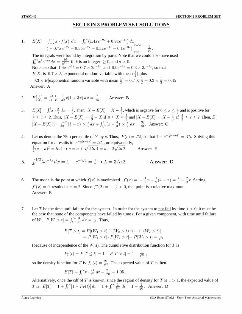
STAM-46 SECTION 3 PROBLEM SET
Actex Learning SOA Exam STAM - Short-Term Actuarial Mathematics
SECTION 3 PROBLEM SET SOLUTIONS
1. IÒ\Ó œ B † 0ÐBÑ .B œ Ð"Þ%B/ !Þ*B/ Ñ .B ∞ !∞ ∞ #B $B
. œ Ð !Þ(B/ !Þ$&/ !Þ$B/ !Þ"/ Ñ œ#B #B $B $B
Bœ!
Bϰ *#!
The integrals were found by integration by parts. Note that we could also have used
if is an integer , and .!∞ 5 +BB / .B œ 5 ! + !5x
+5"
Note also that and , so that"Þ%B/ œ !Þ( ‚ #/ !Þ*/ œ !Þ$ ‚ $/#B #B $B $B
is exponential random variable with mean plusIÒ\Ó !Þ( ‚ IÒ Ó"# exponential random variable with mean !Þ$ ‚ IÒ Ó œ !Þ( ‚ !Þ$ ‚ œ !Þ%&" " "
$ # $ Answer: A
2. . Answer: BI œ † BÐ" $BÑ .B œÒ Ó" " " (\ B $! "&
"$
3. IÒ\Ó œ B † .B œ \ IÒ\Ó œ \ ! Ÿ B Ÿ!
# B % % %# $ $ $. Then, which is negative for and is positive for,
% % % % %$ $ $ $ $Ÿ B Ÿ # \ IÒ\Ó œ \ ! Ÿ \ Ÿ \ IÒ\Ó œ \ Ÿ B Ÿ # IÒ. Thus, if and if . Then, \ IÒ\Ó Ó œ Ð BÑ ‚ .B ÐB Ñ ‚ .B œ! %Î$
%Î$ #%$
B % B $## $ # )" . Answer: C
4. Let us denote the 75th percentile of by . Thus, , so that . Solving this] - JÐ-Ñ œ Þ(& " / œ Þ(& Ð-+Ñ"#
#
equation for results in , or equivalently,- / œ Þ#& Ð-+Ñ"#
#
"# Ð- +Ñ œ 68 % p - œ + # 68 % œ + # 68 ## . Answer: E
5. . Answer: D!"Î$ B Î$ "
#- -/ .B œ " / œ p œ $ 68 #- -
6. The mode is the point at which is maximized. . Setting0ÐBÑ 0 ÐBÑ œ B Ð% BÑ œ Bw " " % #* * * *
0 ÐBÑ œ ! B œ # 0 Ð#Ñ œ !w ww results in . Since , that point is a relative maximum. #*
Answer: E
7. Let be the time until failure for the system. In order for the system to by time , it must beX > !not failthe case that of the components have failed by time . For a given component, with time until failurenone >
of , . Thus,[ TÒ[ >Ó œ .B œ>∞ $ "
B >% $
T ÒX >Ó œ T ÒÐ[ >Ñ ∩ Ð[ >Ñ ∩â ∩ Ð[ >ÑÓ" # (
œ TÒ[ >Ó † T Ò[ >ÓâT Ò[ >Ó œ" # (">#"
(because of independence of the 's). The cumulative distribution function for is[ X3
,J Ð>Ñ œ T ÒX Ÿ >Ó œ " T ÒX >Ó œ " X">#"
so the density function for is . The expected value of is thenX 0 Ð>Ñ œ XX#">##
. IÒX Ó œ > † .> œ œ "Þ!&"∞ #" #"
> #!##
Alternatively, once the cdf of is known, since the region of density for is , the expected value ofX X > "
X IÒX Ó œ " Ò" J Ð>ÑÓ .> œ " .> œ " is . Answer: D " "∞ ∞
X" "> #!#"
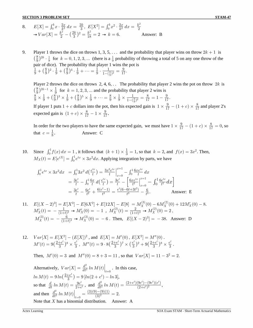
SECTION 3 PROBLEM SET STAM-47
Actex Learning SOA Exam STAM - Short-Term Actuarial Mathematics
8. IÒ\Ó œ B † .B œ ß IÒ\ Ó œ B † .B œ ! !5 5# ##B #5 #B 5
5 $ 5 ## #
#
. Answer: Bp Z +<Ò\Ó œ œ œ # p 5 œ '5 #5 5# $ ")
# #
Ð Ñ#
9. Player 1 throws the dice on throws 1, 3, 5, . . . and the probability that player wins on throw is#5 "
Ð Ñ)*#5 " "
* *† 5 œ !ß "ß #ß $ß ÞÞÞ for (there is a probability of throwing a total of 5 on any one throw of thepair of dice). The probability that player 1 wins the pot is" ) " ) " " " ** * * * * * "("Ð Ñ † † â œ † œ ÞÐ Ñ Ð Ñ# %
)*
#
Player 2 throws the dice on throws 2, 4, 6, . . The probability that player 2 wins the pot on throw is#5
Ð Ñ) "* *
#5" ‚ 5 œ "ß #ß $ß ÞÞÞ for and the probability that player 2 wins is
) " ) " ) " ) " " ) ** * * * * * * * "( "("Ð Ñ‚ ‚ ‚ â œ ‚ ‚ œ œ " ÞÐ Ñ Ð Ñ$ &
)*
#
If player 1 puts dollars into the pot, then his expected gain is and player 2's" - " ‚ Ð" -Ñ ‚* )"( "(
expected gain is Ð" -Ñ ‚ " ‚) *"( "( .
In order for the two players to have the same expected gain, we must have , so" ‚ Ð" -Ñ ‚ œ !* )"( "(
that Answer: C- œ ") .
10. Since , it follows that , so that , and . Then,!
" #0ÐBÑ .B œ " Ð5 "Ñ ‚ œ " 5 œ # 0ÐBÑ œ $B"$
Q Ð>Ñ œ IÒ/ Ó œ / ‚ $B .B\>\ >B #
!
" . Applying integration by parts, we have
! ! !
" " ">B # #
Bœ!
Bœ"
/ ‚ $B .B œ $B . œ .BÐ Ñ/ $B / 'B/> > >
>B # >B >B
œ . œ $/ 'B / $/ 'B/ '/> > > > > >!
"> >B > >B >B
# # !
"
Bœ!
Bœ"
Ð Ñ .B œ œ $/ '/ '
> > > > >'Ð/ "Ñ / Ð''>$> Ñ> >
# $ $ $
> > #
. Answer: E
11. .IÒÐ\ #Ñ Ó œ IÒ\ Ó IÒ'\ Ó IÒ"#\Ó IÒ)Ó œ Q Ð!Ñ 'Q Ð!Ñ "#Q Ð!Ñ )$ $ # wÐ$Ñ Ð#Ñ\ \ \
, Q Ð>Ñ œ p Q Ð!Ñ œ " Q Ð>Ñ œ p Q Ð!Ñ œ # ßw w\ \
Ð#Ñ Ð#Ñ\ \
" #Ð">Ñ Ð">Ñ# $
. Then, . Answer: DQ Ð>Ñ œ p Q Ð!Ñ œ ' IÒÐ\ #Ñ Ó œ $)Ð$Ñ Ð$Ñ\ \
$'Ð">Ñ%
12. , and .Z +<Ò\Ó œ IÒ\ Ó ÐIÒ\ÓÑ IÒ\Ó œ Q Ð!Ñ ß IÒ\ Ó œ Q Ð!Ñ# # w # ww
.Q Ð>Ñ œ * ‚ ß Q Ð>Ñ œ * † ) ‚ * ‚w ) ww ( # )Ð Ñ Ð Ñ Ð Ñ Ð Ñ#/ / #/ / #/ /$ $ $ $ $ $
> > > > > >
Then, and , so that .Q Ð!Ñ œ $ Q Ð!Ñ œ ) $ œ "" Z +<Ò\Ó œ "" $ œ #w ww #
Alternatively, . In this case,Z +<Ò\Ó œ 68QÐ>Ñ..>
#
# >œ!
,68QÐ>Ñ œ * 68 œ * Ò68Ð# / Ñ 68 $ÓÐ Ñ#/$
>>
so that , and , . */ ..> #/ .> Ð#/ Ñ
Ð#/ ÑÐ*/ ÑÐ*/ ÑÐ/ Ñ68QÐ>Ñ œ 68QÐ>Ñ œ
> #
> # > #
> > > >
and then . ..> Ð$Ñ
Ð$ÑÐ*ÑÐ*ÑÐ"Ñ#
# #68QÐ>Ñ œ œ #>œ!
Note that has a binomial distribution. Answer: A\
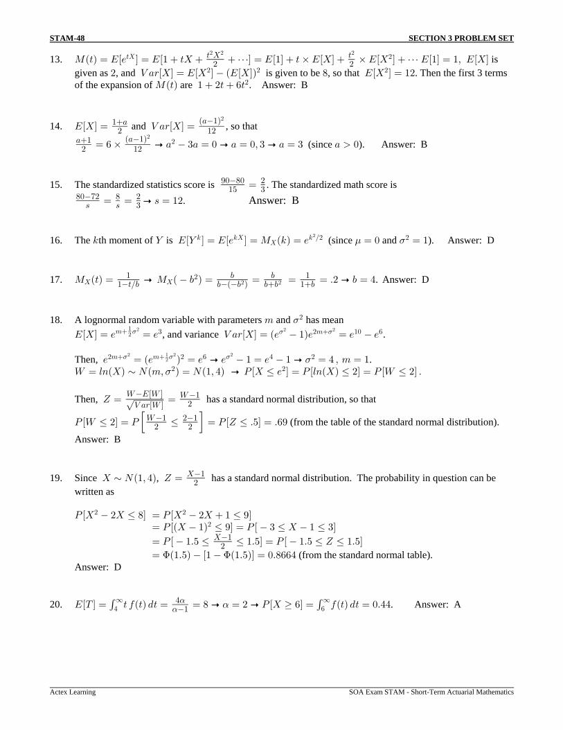
STAM-48 SECTION 3 PROBLEM SET
Actex Learning SOA Exam STAM - Short-Term Actuarial Mathematics
13. isQÐ>Ñ œ IÒ/ Ó œ IÒ" >\ âÓ œ IÒ"Ó > ‚ IÒ\Ó ‚ IÒ\ Ó â IÒ"Ó œ "ß IÒ\Ó>\ #> \ ># #
# # #
given as , and is given to be , so that . Then the first 3 terms# Z +<Ò\Ó œ IÒ\ Ó ÐIÒ\ÓÑ ) IÒ\ Ó œ "## # #
of the expansion of are . Answer: BQÐ>Ñ " #> '>#
14. and , so thatIÒ\Ó œ Z +<Ò\Ó œ"+# "#
Ð+"Ñ#
+"# "#
Ð+"Ñœ ' ‚ p + $+ œ ! p + œ !ß $ p + œ $ + !
## (since ). Answer: B
15. The standardized statistics score is . The standardized math score is*!)! #"& $œ
)!(# ) #= = $œ œ p = œ "#. Answer: B
16. The th moment of is (since and ). Answer: D5 ] IÒ] Ó œ IÒ/ Ó œ Q Ð5Ñ œ / œ ! œ "5 5\ 5 Î# #\
#. 5
17. . Answer: DQ Ð>Ñ œ p Q Ð , Ñ œ œ œ œ Þ# p , œ %\ \#" , , "
">Î, ,Ð, Ñ ,, ",# #
18. A lognormal random variable with parameters and has mean7 5#
, and variance .IÒ\Ó œ / œ / Z +<Ò\Ó œ Ð/ "Ñ/ œ / /7 $ #7 "! '"#5 5 5# # #
Then, ./ œ Ð/ Ñ œ / p / " œ / " p œ % ß 7 œ "#7 7 # ' % #5 5 5# # #"# 5
[ œ 68Ð\Ñ µ RÐ7ß Ñ œ RÐ"ß %Ñ p T Ò\ Ÿ / Ó œ T Ò68Ð\Ñ Ÿ #Ó œ T Ò[ Ÿ #Ó Þ5# #
Then, has a standard normal distribution, so that^ œ œ[IÒ[ Ó
Z +<Ò[ Ó["#
(from the table of the standard normal distribution). T Ò[ Ÿ #Ó œ T Ÿ œ TÒ^ Ÿ Þ&Ó œ Þ'* [" #"# #
Answer: B
19. Since , has a standard normal distribution. The probability in question can be\ µ RÐ"ß %Ñ ^ œ \"#
written as
T Ò\ #\ Ÿ )Ó œ T Ò\ #\ " Ÿ *Ó# #
œ TÒÐ\ "Ñ Ÿ *Ó œ T Ò $ Ÿ \ " Ÿ $Ó#
œ TÒ "Þ& Ÿ Ÿ "Þ&Ó œ T Ò "Þ& Ÿ ^ Ÿ "Þ&Ó\"#
(from the standard normal table). œ Ð"Þ&Ñ Ò" Ð"Þ&ÑÓ œ !Þ)''%F FAnswer: D
20. . Answer: AIÒX Ó œ > 0Ð>Ñ .> œ œ ) p œ # p T Ò\ 'Ó œ 0Ð>Ñ .> œ !Þ%% % '∞ ∞%
"α
α α
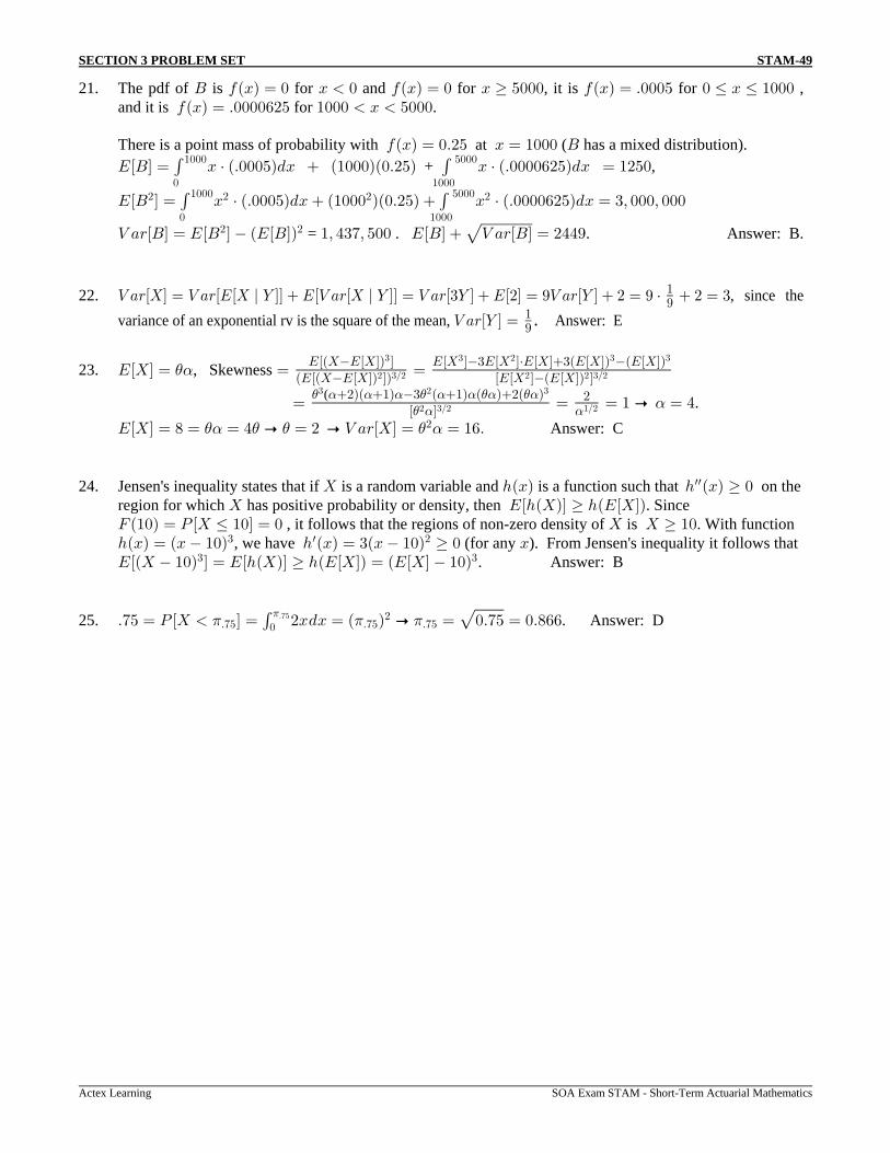
SECTION 3 PROBLEM SET STAM-49
Actex Learning SOA Exam STAM - Short-Term Actuarial Mathematics
21. The pdf of is for and for , it is for ,F 0ÐBÑ œ ! B ! 0ÐBÑ œ ! B &!!! 0ÐBÑ œ Þ!!!& ! Ÿ B Ÿ "!!!and it is for .0ÐBÑ œ Þ!!!!'#& "!!! B &!!!
There is a point mass of probability with at ( has a mixed distribution).0ÐBÑ œ !Þ#& B œ "!!! F
+ ,IÒFÓ œ B † ÐÞ!!!&Ñ.B Ð"!!!ÑÐ!Þ#&Ñ B † ÐÞ!!!!'#&Ñ.B œ "#&! ! "!!!
"!!! &!!!
IÒF Ó œ B † ÐÞ!!!&Ñ.B Ð"!!! ÑÐ!Þ#&Ñ B † ÐÞ!!!!'#&Ñ.B œ $ß !!!ß !!!# # # #
! "!!!
"!!! &!!! = . . Answer: B.Z +<ÒFÓ œ IÒF Ó ÐIÒFÓÑ "ß %$(ß &!! IÒFÓ Z +<ÒFÓ œ #%%*# #
22. Z +<Ò\Ó œ Z +<ÒIÒ\ ± ] ÓÓ IÒZ +<Ò\ ± ] ÓÓ œ Z +<Ò$] Ó IÒ#Ó œ *Z +<Ò] Ó # œ * † # œ $"* , since the
variance of an exponential rv is the square of the mean, Answer: EZ +<Ò] Ó œ "* .
23. , SkewnessIÒ\Ó œ œ œ)αIÒÐ\IÒ\ÓÑ Ó IÒ\ Ó$IÒ\ Ó†IÒ\Ó$ÐIÒ\ÓÑ ÐIÒ\ÓÑ
ÐIÒÐ\IÒ\ÓÑ ÓÑ ÒIÒ\ ÓÐIÒ\ÓÑ Ó
$ $ # $ $
# $Î# # # $Î#
.œ œ œ " p œ %) α α α ) α α )α )α
) α α
$ # $
# $Î# "Î#
( #ÑÐ "Ñ $ Ð "Ñ Ð Ñ#Ð ÑÒ Ó
# α
Answer: CIÒ\Ó œ ) œ œ % p œ # p Z +<Ò\Ó œ œ "'Þ)α ) ) ) α#
24. Jensen's inequality states that if is a random variable and is a function such that on the\ 2ÐBÑ 2 ÐBÑ !ww
region for which has positive probability or density, then . Since\ IÒ2Ð\ÑÓ 2ÐIÒ\ÓÑJ Ð"!Ñ œ T Ò\ Ÿ "!Ó œ ! \ \ "! , it follows that the regions of non-zero density of is . With function2ÐBÑ œ ÐB "!Ñ 2 ÐBÑ œ $ÐB "!Ñ ! B$ w #, we have (for any ). From Jensen's inequality it follows that
. Answer: BIÒÐ\ "!Ñ Ó œ IÒ2Ð\ÑÓ 2ÐIÒ\ÓÑ œ ÐIÒ\Ó "!Ñ$ $
25. . Answer: DÞ(& œ T Ò\ Ó œ #B.B œ Ð Ñ p œ !Þ(& œ !Þ)''1 1 1Þ(& Þ(& Þ(&!# 1Þ(&

STAM-50 SECTION 3 PROBLEM SET
Actex Learning SOA Exam STAM - Short-Term Actuarial Mathematics
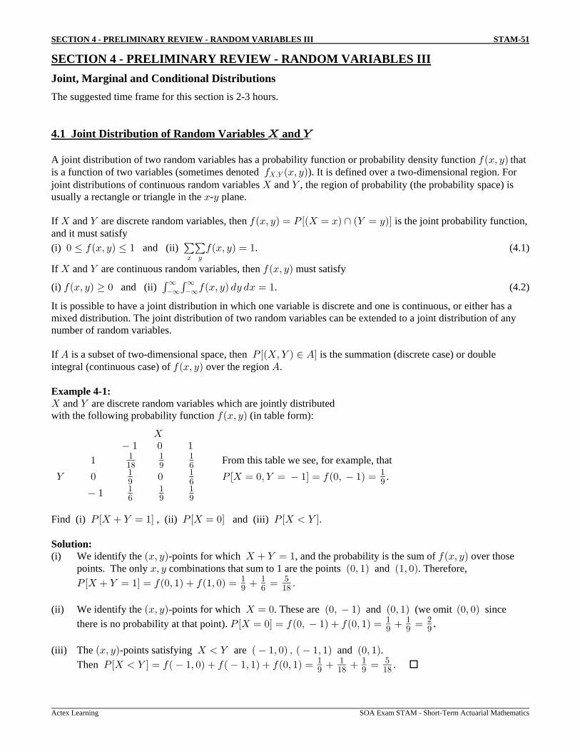
SECTION 4 - PRELIMINARY REVIEW - RANDOM VARIABLES III STAM-51
Actex Learning SOA Exam STAM - Short-Term Actuarial Mathematics
SECTION 4 - PRELIMINARY REVIEW - RANDOM VARIABLES III
Joint, Marginal and Conditional Distributions
The suggested time frame for this section is 2-3 hours.
4.1 Joint Distribution of Random Variables and \ ]
A joint distribution of two random variables has a probability function or probability density function that0ÐBß CÑis a function of two variables (sometimes denoted ). It is defined over a two-dimensional region. For0 ÐBß CÑ\ß]
joint distributions of continuous random variables and , the region of probability (the probability space) is\ ]usually a rectangle or triangle in the - plane.B C
If and are discrete random variables, then is the joint probability function,\ ] 0ÐBß CÑ œ T ÒÐ\ œ BÑ ∩ Ð] œ CÑÓand it must satisfy(i) and (ii) . (4.1)! Ÿ 0ÐBß CÑ Ÿ " 0ÐBß CÑ œ "
B C
If and are continuous random variables, then must satisfy\ ] 0ÐBß CÑ
(i) and (ii) . (4.2)0ÐBß CÑ ! 0ÐBß CÑ .C .B œ " ∞ ∞
∞ ∞
It is possible to have a joint distribution in which one variable is discrete and one is continuous, or either has amixed distribution. The joint distribution of two random variables can be extended to a joint distribution of anynumber of random variables.
If is a subset of two-dimensional space, then is the summation (discrete case) or doubleE TÒÐ\ß ] Ñ − EÓintegral (continuous case) of over the region .0ÐBß CÑ E
Example 4-1:\ ] and are discrete random variables which are jointly distributedwith the following probability function (in table form):0ÐBß CÑ
\ " ! "
From this table we see, for example, that" " " "") * '
.] ! ! T Ò\ œ !ß ] œ "Ó œ 0Ð!ß "Ñ œ" " "* ' *
" " " "' * *
Find (i) , (ii) and (iii) .T Ò\ ] œ "Ó T Ò\ œ !Ó T Ò\ ] Ó
Solution:(i) We identify the -points for which , and the probability is the sum of over thoseÐBß CÑ \ ] œ " 0ÐBß CÑ
points. The only combinations that sum to 1 are the points and . Therefore,Bß C Ð!ß "Ñ Ð"ß !Ñ
T Ò\ ] œ "Ó œ 0Ð!ß "Ñ 0Ð"ß !Ñ œ œ Þ" " &* ' ")
(ii) We identify the -points for which . These are and (we omit sinceÐBß CÑ \ œ ! Ð!ß "Ñ Ð!ß "Ñ Ð!ß !Ñ
there is no probability at that point). T Ò\ œ !Ó œ 0Ð!ß "Ñ 0Ð!ß "Ñ œ œ" " #* * * .
(iii) The -points satisfying are and .ÐBß CÑ \ ] Ð "ß !Ñ ß Ð "ß "Ñ Ð!ß "Ñ
Then T Ò\ ] Ó œ 0Ð "ß !Ñ 0Ð "ß "Ñ 0Ð!ß "Ñ œ œ Þ" " " &* ") * ")
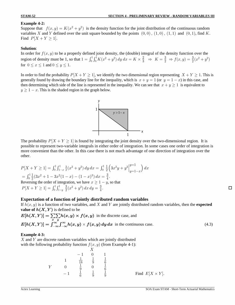
STAM-52 SECTION 4 - PRELIMINARY REVIEW - RANDOM VARIABLES III
Actex Learning SOA Exam STAM - Short-Term Actuarial Mathematics
Example 4-2:Suppose that is the density function for the joint distribution of the continuous random0ÐBß CÑ œ OÐB C Ñ# #
variables and defined over the unit square bounded by the points and , find .\ ] Ð!ß !Ñ ß Ð"ß !Ñ ß Ð"ß "Ñ Ð!ß "Ñ OFind .T Ò\ ] "Ó
Solution:In order for to be a properly defined joint density, the (double) integral of the density function over the0ÐBß CÑ
region of density must be 1, so that " œ OÐB C Ñ .C .B œ O Ê O œ Ê 0ÐBß CÑ œ ÐB C Ñ ! !" " # # # # ‚ # $ $
$ # #for and .! Ÿ B Ÿ " ! Ÿ C Ÿ "
In order to find the probability , we identify the two dimensional region representing . This isT Ò\ ] "Ó \ ] "generally found by drawing the boundary line for the inequality, which is (or ) in this case, andB C œ " C œ " Bthen determining which side of the line is represented in the inequality. We can see that is equivalent toB C "C " B. This is the shaded region in the graph below.
y
1
1x
1y x
The probability is found by integrating the joint density over the two-dimensional region. It isT Ò\ ] "Ópossible to represent two-variable integrals in either order of integration. In some cases one order of integration ismore convenient than the other. In this case there is not much advantage of one direction of integration over theother.
T Ò\ ] "Ó œ ÐB C Ñ .C .B œ $B C C .B ! "B !
" " "$#
# # # $"# Cœ"B
Cœ"
œ Ð$B " $B Ð" BÑ Ð" BÑ Ñ .B œ Þ!
" # # $" $# %
Reversing the order of integration, we have , so thatB " C
T Ò\ ] "Ó œ ÐB C Ñ .B .C œ Þ ! "C
" " # #$ $# %
Expectation of a function of jointly distributed random variablesIf is a function of two variables, and and are jointly distributed random variables, then the 2ÐBß CÑ \ ] expectedvalue of 2Ð\ß] Ñ is defined to be
IÒ2Ð\ß] ÑÓ œ 2ÐBß CÑ ‚ 0ÐBß CÑB C
in the discrete case, and
IÒ2Ð\ß] ÑÓ œ 2ÐBß CÑ 0ÐBß CÑ .C .B ∞ ∞
∞ ∞‚ in the continuous case. (4.3)
Example 4-3:\ ] and are discrete random variables which are jointly distributedwith the following probability function (from Example 4-1):0ÐBß CÑ \ " ! "
" " " "") * '
] ! !" "* '
Find . " IÒ\ ‚ ] Ó" " "' * *
SECTION 4 - PRELIMINARY REVIEW - RANDOM VARIABLES III STAM-53
Actex Learning SOA Exam STAM - Short-Term Actuarial Mathematics
Solution:IÒ\] Ó œ BC 0ÐBß CÑ œ Ð "ÑÐ"ÑÐ Ñ Ð "ÑÐ!ÑÐ Ñ Ð "ÑÐ "ÑÐ Ñ
B C‚ " " "
") * '
Ð!ÑÐ"ÑÐ Ñ Ð!ÑÐ!ÑÐ!Ñ Ð!ÑÐ "ÑÐ Ñ Ð"ÑÐ"ÑÐ Ñ Ð"ÑÐ!ÑÐ Ñ Ð"ÑÐ "ÑÐ Ñ œ" " " " " "* * ' ' * ' . Note that
the summation is taken over all pairs in the joint distribution. ÐBß CÑ
Example 4-4:Suppose that is the density function for the joint distribution of the continuous random0ÐBß CÑ œ ÐB C Ñ$
## #
variables and defined over the unit square defined on the region and . Find\ ] ! Ÿ B Ÿ " ! Ÿ C Ÿ "IÒ\ ] Ó# # .Solution:IÒ\ ] Ó œ ÐB C Ñ ‚ 0ÐBß CÑ .C .B œ ÐB C ÑÐ ÑÐB C Ñ .C .B# # # # # # # #
! ! ! !" " " " $
#
œ Ð"Þ&B B Þ$Ñ .B œ!" % # "%
"& .
4.2 Marginal distribution of found from a joint distribution of and \ \ ]If and have a joint distribution with joint density or probability function , then the \ ] 0ÐBß CÑ marginaldistribution of \ has a probability function or density function denoted , which is equal to0 ÐBÑ\
0 ÐBÑ œ 0ÐBß CÑ\C
in the discrete case, and is equal to
0 ÐBÑ œ 0ÐBß CÑ .C\ ∞
∞ in the continuous case. (4.4)
The density function for the marginal distribution of is found in a similar way, is equal to either] 0 ÐCÑ]
0 ÐCÑ œ 0ÐBß CÑ 0 ÐCÑ œ 0ÐBß CÑ .B] ]B
∞
∞ or .
For instance, in the discrete case. What we are doing is "adding up" the probability for all0 Ð"Ñ œ 0Ð"ß CÑ\C
points whose -value is 1 to get the overall probability the is 1.B \
Marginal probability functions and marginal density functions must satisfy all the requirements of probability anddensity functions. A marginal probability function must sum to 1 over all points of probability and a marginaldensity function must integrate to 1. The marginal distribution of describes the behavior of alone without\ \reference to (and same for marginal of ).] ]
Example 4-5:Find the marginal distributions of and for the joint distribution in Example 4-1 .\ ]
Solution:The joint distribution was given as \ " ! "
" " " "") * '
] ! !" "* '
" " " "' * *
To find the marginal probability function for , we first note that can be or .\ \ " ß ! "We wish to find and .0 Ð "Ñ œ T Ò\ œ "Ó ß 0 Ð!Ñ 0 Ð"Ñ\ \ \
As noted above, to find we sum over the other variable :0 ÐBÑ ]\
0 Ð "Ñ œ 0Ð "ß CÑ œ 0Ð "ß "Ñ 0Ð "ß !Ñ 0Ð "ß "Ñ œ œ\C
all
" " " "' * ") $ .
STAM-54 SECTION 4 - PRELIMINARY REVIEW - RANDOM VARIABLES III
Actex Learning SOA Exam STAM - Short-Term Actuarial Mathematics
In a similar way we get and .0 Ð!Ñ œ ! œ 0 Ð"Ñ œ œ\ \" " # " " " %* * * * ' ' *
In Example 4-1 we saw that .T Ò\ œ !Ó œ #*
What we were finding was the marginal probability that was just found here .0 Ð!Ñ\
Note also that .all B
\ \ \ \0 ÐBÑ œ 0 Ð "Ñ 0 Ð!Ñ 0 Ð"Ñ œ œ "" # %$ * *
This verifies that satisfies the requirements of a probability function. The marginal probability function of0 ÐBÑ\
] B is found in the same way, except that we sum over (across each row in the table above).0 Ð "Ñ œ œ 0 Ð!Ñ œ ! œ 0 Ð"Ñ œ œ] ] ]
" " " ( " " & " " " "' * * ") * ' ") ") * ' $ , and .
Example 4-6:Find the marginal distributions of and for the joint distribution in Example 4-2 .\ ]Solution:The joint density function is for and .0ÐBß CÑ œ ÐB C Ñ ! Ÿ B Ÿ " ! Ÿ C Ÿ "$
## #
The marginal density function of is found by integrating out the other variable .\ C
0 ÐBÑ œ 0ÐBß CÑ .C œ 0ÐBß CÑ .C œ ÐB C Ñ .C œ B ! Ÿ B Ÿ "\ C ! !" " # # #
all $ $ "# # # for .
We can verify that this is a proper density function by checking that .!
"\0 ÐBÑ .B œ "
In a similar way, for . 0 ÐCÑ œ C ! Ÿ C Ÿ "]#$ "
# #
4.3 Independence of random variables andX YRandom variables and with density functions and are said to be independent (or stochastically\ ] 0 ÐBÑ 0 ÐCÑ\ ]
independent) if the probability space is rectangular ( , where the endpoints can be infinite)+ Ÿ B Ÿ , ß - Ÿ C Ÿ .and if the joint density function is of the form
0ÐBß CÑ œ 0 ÐBÑ ‚ 0 ÐCÑ\ ] . (4.5)
If and are independent, then for any functions and ,\ ] 1 2
IÒ1Ð\Ñ 2Ð] ÑÓ œ IÒ1Ð\ÑÓ IÒ2Ð] ÑÓ IÒ\ ] Ó œ IÒ\Ó IÒ] Ó‚ ‚ ‚ ‚ , and in particular, . (4.6)
For the discrete joint distribution in Example 4-1 we can see that and are not independent, because, for\ ]
instance, . For the continuous joint distribution of Example0Ð "ß "Ñ œ Á œ 0 Ð "Ñ 0 Ð "Ñ" " (' $ ")‚ ‚\ ]
4-2, we see that0ÐBß CÑ œ ÐB C Ñ Á Ð B ÑÐ C Ñ œ 0 ÐBÑ 0 ÐCÑ \ ]$ $ " $ "
# # # # ## # # #
\ ]‚ , so and are not independent.
Example 4-7:Suppose that and are independent continuous random variables with the following density functions:\ ]0 ÐBÑ œ " ! B " 0 ÐCÑ œ #C ! C "\ ]for and for .Find .T Ò] \ÓSolution:Since and are independent, the density function of the joint distribution of and is\ ] \ ]0ÐBß CÑ œ 0 ÐBÑ 0 ÐCÑ œ #C \ ]\ ]‚ , and is defined on the rectangle created by the intervals for and , which, in
this case, is the unit square. . T Ò] \Ó œ #C .C .B œ ! !" B "
$
SECTION 4 - PRELIMINARY REVIEW - RANDOM VARIABLES III STAM-55
Actex Learning SOA Exam STAM - Short-Term Actuarial Mathematics
4.4 Conditional distribution of given Y X = xConditional distributions are very important in the loss models and credibility material and must be understoodwell..
The way in which a conditional distribution is defined follows the basic definition of conditional probability,
T ÒElFÓ œT ÒE∩FÓT ÒFÓ . In fact, given discrete joint distribution, this is exactly how a conditional distribution is defined.
Example 4-1 described a discrete joint distribution of and , and then Example 4-5 showed how to formulate the\ ]marginal distributions of and . We now wish to formulate a conditional distribution. For instance, for the joint\ ]distribution of Example 4-1, suppose we wish to describe the conditional distribution of given . What we are\ ] œ "trying to describe are conditional probabilities of the form .T Ò\ œ Bl] œ "Ó
We find these conditional probabilities in the usual way that conditional probability is defined.
.T Ò\ œ "l] œ "Ó œT ÒÐ\œ"Ñ∩Ð] œ"ÑÓ
T Ò] œ"Ó
The denominator is the marginal probability that , . The numerator is the joint probability] œ " 0 Ð"Ñ œ]"$
0Ð "ß "Ñ œ "") , which is found in the joint probability table. Then,
. We would denote this conditional probabilityT Ò\ œ "l] œ "Ó œ0Ð"ß"Ñ "Î")0 Ð"Ñ "Î$ '
"]
œ œ
0 Ð "l] œ "Ñ 0 Ð!l] œ "Ñ œ œ\l] \l]. In a similar way, we can get , and0Ð!ß"Ñ "Î*0 Ð"Ñ "Î$ $
"]
œ
0 Ð"l] œ "Ñ œ œ \ ] œ "\l]0Ð"ß"Ñ "Î'0 Ð"Ñ "Î$ #
"]
œ . This completely describes the conditional distribution of given .
As with any discrete distribution, probabilities must add to 1, and this is the case for this conditional distribution,since0 Ð "l] œ "Ñ 0 Ð!l] œ "Ñ 0 Ð"l] œ "Ñ œ œ "\l] \l] \l]
" " "' $ # .
A conditional distribution satisfies all the same properties of any distribution. We can find a conditional mean, aconditional variance, etc. For instance, the conditional mean of given in the example we have just been\ ] œ "considering is
IÒ\l] œ "Ó œ B 0 ÐBl] œ "Ñ+66 BD ‚ \l]
œ Ð "Ñ0 Ð "l] œ "Ñ Ð!Ñ0 Ð!l] œ "Ñ Ð"Ñ0 Ð"l] œ "Ñ\l] \l] \l]
œ Ð "ÑÐ Ñ Ð!ÑÐ Ñ Ð"ÑÐ Ñ œ Þ" " " "' $ # $
We can find the second conditional moment in a similar way, . Then theIÒ\ l] œ "Ó œ B 0 ÐBl] œ "Ñ+66 B
# #\l]D ‚
conditional variance would be .Z +<Ò\l] œ "Ó œ IÒ\ l] œ "Ó ÐIÒ\l] œ "ÓÑ# #
The expression for conditional probability that was used above in the discrete case was
0 ÐBl] œ CÑ œ\l]0ÐBßCÑ0 ÐCÑ]
. This can be applied to find a conditional distribution of given also, so that] \ œ B
we define
. (4.7)0 ÐCl\ œ BÑ œ] l\0ÐBßCÑ0 ÐBÑ\
We also apply this same algebraic form to define the conditional density in the continuous case, with 0ÐBß CÑbeing the joint density and being the marginal density. In the continuous case, the conditional mean of 0 ÐBÑ ]\
given would be\ œ B (4.8)IÒ] l\ œ BÓ œ C ‚ 0 ÐCl\ œ BÑ .C ] l\
STAM-56 SECTION 4 - PRELIMINARY REVIEW - RANDOM VARIABLES III
Actex Learning SOA Exam STAM - Short-Term Actuarial Mathematics
where the integral is taken over the appropriate interval for the conditional distribution of given . The] \ œ Bconditional density/probability is also written as , or .0 ÐClBÑ 0ÐClBÑ] l\
If and are independent random variables, then and ,\ ] 0 ÐCl\ œ BÑ œ 0 ÐCÑ 0 ÐBl] œ CÑ œ 0 ÐBÑ] l\ \l]] \
which indicates that the density of does not depend on and vice-versa. The conditional density function must] \satisfy the usual requirement of a density function,∞∞
] l\ \0 ÐClBÑ .C œ " \ 0 ÐBÑ . Note also that if the marginal density of is known, , and the conditional densityof given is also known, , then the joint density of and can be formulated as] \ œ B 0 ÐCl\ œ BÑ \ ]] l\
(4.9)0ÐBß CÑ œ 0 ÐCl\ œ BÑ ‚ 0 ÐBÑ Þ] l\ \
Example 4-8:Find the conditional distribution of given for the joint distribution of Example 4-1. Find the] \ œ "conditional expectation of given .] \ œ "
Solution:The marginal probability function for was found in Example 4-5, where it was found that . The\ 0 Ð "Ñ œ\
"$
conditional probability function of given is . Then,] \ œ " 0 ÐCl\ œ "Ñ œ œ] l\0Ð"ßCÑ 0Ð"ßCÑ0 Ð"Ñ "Î$\
0 Ð "l\ œ "Ñ œ œ œ ß 0 Ð!l\ œ "Ñ œ œ œ ß] l\ ] l\0Ð"ß"Ñ "Î' 0Ð"ß!Ñ "Î*
"Î$ "Î$ # "Î$ "Î$ $" "
and .0 Ð"l\ œ "Ñ œ œ œ] l\0Ð"ß"Ñ "Î")
"Î$ "Î$ '"
IÒ] l\ œ "Ó œ C 0 ÐCl\ œ "Ñ œ Ð "ÑÐ Ñ Ð!ÑÐ Ñ Ð"ÑÐ Ñ œ all C
] l\‚ " " " "# $ ' $ .
Example 4-9:Find the conditional density and conditional expectation and conditional variance of given for the\ ] œ Þ$joint distribution of Example 4-2.Solution:
0 ÐBl] œ !Þ$Ñ œ œ œ\l]0ÐBßÞ$Ñ0 ÐÞ$Ñ !Þ'$&
ÐB !Þ$ Ñ ÐB !Þ!*Ñ
Ð!Þ$Ñ ]
$ $# #
# # #
$ "# #
# . The conditional expectation is
IÒ\l] œ !Þ$Ó œ B † 0 ÐBl] œ !Þ$Ñ .B œ B † .B œ !Þ'*( ! !
" "\l]
$#
#ÐB !Þ!*Ñ
!Þ'$& .
The conditional second moment of given is\ ] œ !Þ$
IÒ\ l] œ !Þ$Ó œ B 0 ÐBl] œ !Þ$Ñ .B œ B .B œ !Þ&%$# # #! !" "
\l] ‚ ‚$#
#ÐB !Þ!*Ñ
!Þ'$& .
The conditional variance is
. Z +<Ò\l] œ !Þ$Ó œ IÒ\ l] œ !Þ$Ó ÐIÒ\l] œ !Þ$ÓÑ œ !Þ&%$ Ð!Þ'*(Ñ œ !Þ!&(# # #
We can construct the joint density from knowing the conditional density and the marginal0ÐBß CÑ 0 ÐClBÑ] l\
density using the relationship . When doing this, care must be taken to ensure0 ÐBÑ 0ÐBß CÑ œ 0ÐClBÑ 0 ÐBÑ\ \‚that proper two-dimensional region is being formulated for the joint distribution.
SECTION 4 - PRELIMINARY REVIEW - RANDOM VARIABLES III STAM-57
Actex Learning SOA Exam STAM - Short-Term Actuarial Mathematics
Example 4-10:Suppose that has a continuous distribution with pdf on the interval , and \ 0 ÐBÑ œ #B Ð!ß "Ñ 0 ÐBÑ œ !\ \
elsewhere. Suppose that is a continuous random variable such that the conditional distribution of given] ]\ œ B Ð!ß BÑ ] is uniform on the interval . Find the mean and variance of (the marginal distribution of) .Solution:We find the unconditional (marginal) distribution of . We are given for , and] 0 ÐBÑ œ #B ! B "\
0 ÐCl\ œ BÑ œ ! C B] l\"B for .
Then, for .0ÐBß CÑ œ 0ÐClBÑ 0 ÐBÑ œ ‚ #B œ # ! C B "‚ \"B
The unconditional (marginal) distribution of has pdf.]
0 ÐCÑ œ 0ÐBß CÑ .B œ # .B œ #Ð" CÑ ! C " 0 ÐCÑ !] ]∞ C∞ " for (and is elsewhere).
Then , , andIÒ] Ó œ C † #Ð" CÑ .C œ IÒ] Ó œ C † #Ð" CÑ .C œ ! !" "# #" "
$ '
Z +<Ò] Ó œ IÒ] Ó ÐIÒ] ÓÑ œ Ð Ñ œ# # #" " "' $ ") .
The idea applied in Example 4-10 is quite important in the continuous Bayesian credibility approach that will becovered later in the study guide.
4.5 Covariance Between Random Variables andX YIf random variables and are jointly distributed with joint density/probability function , the covariance\ ] 0ÐBß CÑbetween and is\ ]
G9@Ò\ß ] Ó œ IÒÐ\ IÒ\ÓÑÐ] IÒ] ÓÑÓ œ IÒÐ\ ÑÐ] ÑÓ œ IÒ\] Ó IÒ\Ó IÒ] ÓÞ. .\ ] ‚ (4.10)Note that . If and are independent, thenG9@Ò\ß\Ó œ Z +<Ò\Ó \ ]
IÒ\ † ] Ó œ IÒ\Ó † IÒ] Ó G9@Ò\ß ] Ó œ ! and . (4.11)
For constants and random variables and ,+ß ,ß -ß .ß /ß 0 \ß ] ß ^ [
G9@Ò+\ ,] - ß .^ /[ 0Ó œ +.G9@Ò\ß ^Ó +/G9@Ò\ß[ Ó ,.G9@Ò] ß ^Ó ,/G9@Ò] ß[ Ó
(4.12)
An important application of the covariance is in finding the variance of the sum of and . Suppose that , \ ] + ,
and are constants. Then-
Z +<Ò+\ ,] -Ó œ + Z +<Ò\Ó , Z +<Ò] Ó #+,G9@Ò\ß ] Ó# # (4.13)
If and are independent, then .\ ] Z +<Ò\ ] Ó œ Z +<Ò\Ó Z +<Ò] Ó
If are independent, then .\ ß\ ß ÞÞÞß\ Z +<Ò \ Ó œ Z +<Ò\ Ó" # 8 3 33œ" 3œ"
8 8 (4.14)
If are independent, and if , then the moment generating function of is\ ß\ ß ÞÞÞß\ W œ \ W" # 8 33œ"
8 . Q Ð>Ñ œ Q Ð>ÑW \
3œ"
83 (4.15)
STAM-58 SECTION 4 - PRELIMINARY REVIEW - RANDOM VARIABLES III
Actex Learning SOA Exam STAM - Short-Term Actuarial Mathematics
4.6 Coefficient of correlation between random variables andX YThe coefficient of correlation between random variables and is defined to be\ ]
3 3Ð\ß] Ñ œ œ\ß]G9@Ò\ß] Ó5 5\ ] , (4.16)
where and are the standard deviations of and respectively. Note that always.5 5 3\ ] \ß]\ ] " Ÿ Ÿ "
Example 4-11:Find for the jointly distributed discrete random variables in Example 4-1 above.G9@Ò\ß ] ÓSolution:G9@Ò\ß ] Ó œ IÒ\] Ó IÒ\Ó IÒ] Ó IÒ\] Ó œ‚ . In Example 4-3 it was found that ."
'
The marginal probability function for is ,\ TÒ\ œ "Ó œ œ" " " %' ' * *
T Ò\ œ !Ó œ T Ò\ œ "Ó œ \ IÒ\Ó œ Ð"ÑÐ Ñ Ð!ÑÐ Ñ Ð "ÑÐ Ñ œ# " % # " "* $ * * $ * and , and the mean of is .
In a similar way, the probability function of is found to be and] T Ò] œ "Ó œ ß T Ò] œ !Ó œ ß" &$ ")
T Ò] œ "Ó œ ß IÒ] Ó œ G9@Ò\ß ] Ó œ Ð ÑÐ Ñ œ( " " " " "%") ") ' * ") )"with a mean of . Then, .
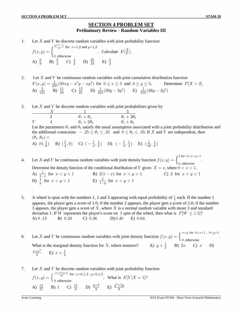
SECTION 4 PROBLEM SET STAM-59
Actex Learning SOA Exam STAM - Short-Term Actuarial Mathematics
SECTION 4 PROBLEM SETPreliminary Review - Random Variables III
1. Let and be discrete random variables with joint probability function\ ]
. Calculate .0ÐBß CÑ œ IÒ Ó#B"C
* for and
otherwise
Bœ"ß# Cœ"ß#
!ß
\]
A) B) C) D) E) ) & % #& &* % $ ") $
2. Let and be continuous random variables with joint cumulative distribution function\ ]
JÐBß CÑ œ Ð#!BC B C BC Ñ ! Ÿ B Ÿ & ! Ÿ C Ÿ & T Ò\ #Ó"#&!
# # for and . Determine .
A) B) C) D) E) $ "" "# " ""#& &! #& #&! #&!Ð$*C $C Ñ Ð$'C #C Ñ# #
3. Let and be discrete random variables with joint probabilities given by\ ] \ " & # #) ) ) )" # " #
] % # ) ) ) )" # " #
Let the parameters and satisfy the usual assumption associated with a joint probability distribution and) )" #
the additional constraints and . If and are independent, then Þ#& Ÿ Ÿ Þ#& ! Ÿ Ÿ Þ$& \ ]) )" #
Ð ß Ñ œ) )" #
A) B) C) D) E) Ð!ß Ñ Ð ß !Ñ Ð ß Ñ Ð ß Ñ Ð ß Ñ" " " " " " "' % $ ) % "' )
"%
4. .Let and be continuous random variables with joint density function \ ] 0ÐBß CÑ œ # !BC"for
!, otherwise
Determine the density function of the conditional distribution of given , where .] \ œ B ! B "
A) for B) for C) for ""B B C " #Ð" BÑ B C " # B C "
D) for E) for " "C "CB C " B C "
5. A wheel is spun with the numbers 1, 2 and 3 appearing with equal probability of each. If the number 1"$
appears, the player gets a score of 1.0; if the number 2 appears, the player gets a score of 2.0; if the number3 appears, the player gets a score of , where is a normal random variable with mean 3 and standard\ \deviation 1. If represents the player's score on 1 spin of the wheel, then what is ?[ TÒ[ Ÿ "Þ&Ó
A) B) C) D) E) ! Þ"$ !Þ$$ !Þ$' !Þ%! !Þ'%
6. Let and be continuous random variables with joint density function .\ ] 0ÐBß CÑ œ for BC !B" ß !C"
!ß otherwise
What is the marginal density function for where nonzero? A) B) C) D)\ß C #B B"#
BB "# #
#
E) B
7. Let and be discrete random variables with joint probability function\ ]
. What is ?0ÐBß CÑ œ IÒ] l\ œ "Ó for
otherwise
ÐB"ÑÐC#Ñ&% Bœ!ß"ß# à Cœ!ß"ß#
!ß
A) B) C) D) E) "" ""#( * * *
C# C #C"
#
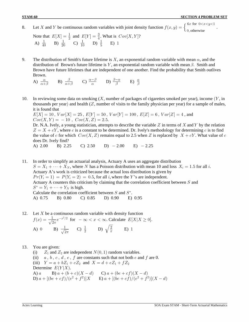
STAM-60 SECTION 4 PROBLEM SET
Actex Learning SOA Exam STAM - Short-Term Actuarial Mathematics
8. Let and be continuous random variables with joint density function .\ ] 0ÐBß CÑ œ for
otherwise
'B !BC"
!ß
Note that and . What is ?IÒ\Ó œ IÒ] Ó œ G9@Ò\ß ] Ó" $# %
A) B) C) D) E) " " " "%! #! "! & "
9. The distribution of Smith's future lifetime is , an exponential random variable with mean , and the\ αdistribution of Brown's future lifetime is , an exponential random variable with mean . Smith and] "Brown have future lifetimes that are independent of one another. Find the probability that Smith outlivesBrown.
A) B) C) D) E) α αα " α " α " "
" α " " α
10. In reviewing some data on smoking ( , number of packages of cigarettes smoked per year), income , in\ Ð]thousands per year and health ( , number of visits to the family physician per year) for a sample of males,Ñ ^it is found that
, andIÒ\Ó œ "! ß Z +<Ò\Ó œ #& ß IÒ] Ó œ &! ß Z +<Ò] Ó œ "!! ß IÒ^Ó œ ' ß Z +<Ò^Ó œ %G9@Ð\ß ] Ñ œ "! ß G9@Ð\ß^Ñ œ #Þ&.
Dr. N.A. Ively, a young statistician, attempts to describe the variable in terms of and by the relation^ \ ]^ œ \ -] - -, where is a constant to be determined. Dr. Ively's methodology for determining is to findthe value of for which remains equal to 2.5 when is replaced by . What value of - G9@Ð\ß^Ñ ^ \ -] -does Dr. Ively find?
A) 2.00 B) 2.25 C) 2.50 D) 2.00 E) 2.25
11. In order to simplify an actuarial analysis, Actuary A uses an aggregate distribution , where has a Poisson distribution with mean 10 and loss for all .W œ \ â\ R \ œ "Þ& 3" R 3
Actuary A’s work is criticized because the actual loss distribution is given by , for all , where the ’s are independent.T<Ð] œ "Ñ œ TÐ] œ #Ñ œ !Þ& 3 ]3 3
Actuary A counters this criticism by claiming that the correlation coefficient between andWW œ ] â ]‡
" R is high. Calculate the correlation coefficient between and .W W‡
A) 0.75 B) 0.80 C) 0.85 D) 0.90 E) 0.95
12. Let be a continuous random variable with density function\
for . Calculate .0ÐBÑ œ / ∞ B ∞ IÒ\l\ !Ó"
# 1B Î##
A) B) C) D) E) ! "" " ##21 1
13. You are given: (i) and are independent random variables.^ ^ RÐ!ß "Ñ" #
(ii) are constants such that not both and are 0.+ ß , ß - ß . ß / ß 0 / 0 (iii) and ] œ + ,^ -^ \ œ . /^ 0^" # " #
Determine .IÐ] l\Ñ A) B) C) + + Ð, -ÑÐ\ .Ñ + Ð,/ -0ÑÐ\ .Ñ D) E) + ÒÐ,/ -0ÑÎÐ/ 0 ÑÓ\ + ÒÐ,/ -0ÑÎÐ/ 0 ÑÓÐ\ .Ñ# # # #
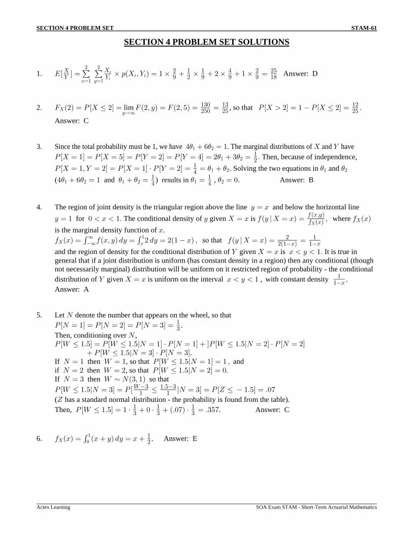
SECTION 4 PROBLEM SET STAM-61
Actex Learning SOA Exam STAM - Short-Term Actuarial Mathematics
SECTION 4 PROBLEM SET SOLUTIONS
1. Answer: DIÒ Ó œ ‚ :Ð\ ß ] Ñ œ " ‚ ‚ # ‚ " ‚ œ\ # " " % # #&] ] * # * * * ")
\ Bœ" Cœ"
# #
3 33
3
2. , so that J Ð#Ñ œ T Ò\ Ÿ #Ó œ JÐ#ß CÑ œ JÐ#ß &Ñ œ œ T Ò\ #Ó œ " T Ò\ Ÿ #Ó œ Þ\CÄ∞lim "$! "$ "#
#&! #& #&
Answer: C
3. Since the total probability must be 1, we have . The marginal distributions of and have% ' œ " \ ]) )" #
T Ò\ œ "Ó œ T Ò\ œ &Ó œ T Ò] œ #Ó œ T Ò] œ %Ó œ # $ œ Þ) )" #"# Then, because of independence,
T Ò\ œ "ß ] œ #Ó œ T Ò\ œ "Ó † T Ò] œ #Ó œ œ "% ) ) ) )" # " #. Solving the two equations in and
( and ) results in , . Answer: B% ' œ " œ œ œ !) ) ) ) ) )" # " # " #" "% %
4. The region of joint density is the triangular region above the line and below the horizontal lineC œ B
C œ " ! B "Þ C \ œ B 0ÐC l\ œ BÑ œ ß 0 ÐBÑ for The conditional density of given is where 0ÐBßCÑ0 ÐBÑ\
\
is the marginal density function of .B so that 0 ÐBÑ œ 0ÐBß CÑ .C œ # .C œ #Ð" BÑ ß 0ÐC l\ œ BÑ œ œ\ ∞ B
∞ " # "#Ð"BÑ "B
and the region of density for the conditional distribution of given is It is true in] \ œ B B C "Þgeneral that if a joint distribution is uniform (has constant density in a region) then any conditional (thoughnot necessarily marginal) distribution will be uniform on it restricted region of probability - the conditionaldistribution of given is uniform on the interval , with constant density . ] \ œ B B C " "
"BAnswer: A
5. Let denote the number that appears on the wheel, so thatR
.T ÒR œ "Ó œ T ÒR œ #Ó œ T ÒR œ $Ó œ "$
Then, conditioning over ,R T Ò[ Ÿ "Þ&Ó œ T Ò[ Ÿ "Þ&lR œ "Ó † T ÒR œ "Ó ÓT Ò[ Ÿ "Þ&lR œ #Ó † T ÒR œ #Ó . TÒ[ Ÿ "Þ&lR œ $Ó † T ÒR œ $Ó If then , so that andR œ " [ œ " T Ò[ Ÿ "Þ&lR œ "Ó œ " ß if then , so that .R œ # [ œ # T Ò[ Ÿ "Þ&lR œ #Ó œ ! If then so thatR œ $ [ µ RÐ$ß "Ñ
T Ò[ Ÿ "Þ&lR œ $Ó œ T Ò Ÿ lR œ $Ó œ T Ò^ Ÿ "Þ&Ó œ Þ!([$ "Þ&$" "
( has a standard normal distribution - the probability is found from the table).^
Then, . Answer: CT Ò[ Ÿ "Þ&Ó œ " † ! † ÐÞ!(Ñ † œ Þ$&(" " "$ $ $
6. . Answer: E0 ÐBÑ œ ÐB CÑ .C œ B \ !
" "#
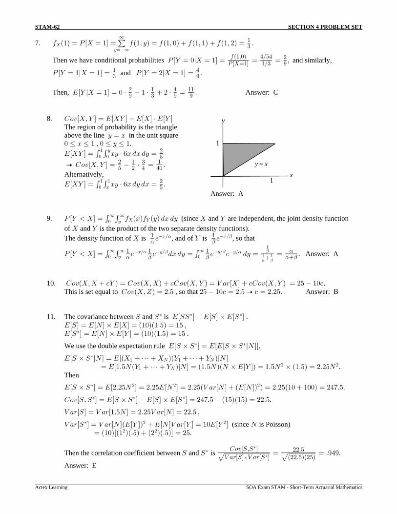
STAM-62 SECTION 4 PROBLEM SET
Actex Learning SOA Exam STAM - Short-Term Actuarial Mathematics
7. .0 Ð"Ñ œ T Ò\ œ "Ó œ 0Ð"ß CÑ œ 0Ð"ß !Ñ 0Ð"ß "Ñ 0Ð"ß #Ñ œ\Cœ∞
∞ "$
Then we have conditional probabilities and similarly,T Ò] œ !l\ œ "Ó œ œ œ ß0Ð"ß!Ñ %Î&%T Ò\œ"Ó "Î$ *
#
T Ò] œ "l\ œ "Ó œ T Ò] œ #l\ œ "Ó œ" %$ *and .
Then, Answer: CIÒ] l\ œ "Ó œ ! † " † # † œ Þ# " % ""* $ * *
8. G9@Ò\ß ] Ó œ IÒ\] Ó IÒ\Ó † IÒ] Ó The region of probability is the triangle
above the line in the unit squareC œ B! Ÿ B Ÿ " ! Ÿ C Ÿ " , .
IÒ\] Ó œ BC † 'B .B .C œ ! !" C #
&
.p G9@Ò\ß ] Ó œ † œ# " $ "& # % %!
Alternatively, . IÒ\] Ó œ BC † 'B .C .B œ
! B
" " #&
y
x
1
1
y x
Answer: A
9. (since and are independent, the joint density functionT Ò] \Ó œ 0 ÐBÑ0 ÐCÑ .B .C \ ] ! C
∞ ∞\ ]
of and is the product of the two separate density functions).\ ]
The density function of is , and of is , so that\ / ] /" "α "
BÎ BÎα "
. Answer: AT Ò] \Ó œ / / .B .C œ / / .C œ œ ! C !
∞ ∞ ∞BÎ CÎ CÎ CÎ" " " α " " α "
αα " " α"
" ""
α "
10. .G9@Ð\ß\ -] Ñ œ G9@Ð\ß\Ñ -G9@Ð\ß ] Ñ œ Z +<Ò\Ó -G9@Ð\ß ] Ñ œ #& "!- This is set equal to , so that . Answer: BG9@Ð\ß^Ñ œ #Þ& #& "!- œ #Þ& p - œ #Þ#&
11. The covariance between and is .W W IÒWW Ó IÒWÓ ‚ IÒW Ó‡ ‡ ‡
IÒWÓ œ IÒRÓ ‚ IÒ\Ó œ Ð"!ÑÐ"Þ&Ñ œ "& ß .IÒW Ó œ IÒRÓ ‚ IÒ] Ó œ Ð"!ÑÐ"Þ&Ñ œ "&‡
We use the double expectation rule .IÒW ‚ W Ó œ IÒIÒW ‚ W lRÓÓ‡ ‡
IÒW ‚ W lRÓ œ IÒÐ\ â\ ÑÐ] â ] ÑlRÓ‡" R " R
.œ IÒ"Þ&RÐ] â ] ÑlRÓ œ Ð"Þ&RÑÐR ‚ IÒ] ÓÑ œ "Þ&R ‚ Ð"Þ&Ñ œ #Þ#&R" R# #
Then
IÒW ‚ W Ó œ IÒ#Þ#&R Ó œ #Þ#&IÒR Ó œ #Þ#&ÐZ +<ÒRÓ ÐIÒRÓÑ Ñ œ #Þ#&Ð"! "!!Ñ œ #%(Þ&Þ‡ # # #
.G9@ÒWß W Ó œ IÒW ‚ W Ó IÒWÓ ‚ IÒW Ó œ #%(Þ& Ð"&ÑÐ"&Ñ œ ##Þ&‡ ‡ ‡
Z +<ÒWÓ œ Z +<Ò"Þ&RÓ œ #Þ#&Z +<ÒRÓ œ ##Þ& ß
(since is Poisson)Z +<ÒW Ó œ Z +<ÒRÓÐIÒ] ÓÑ IÒRÓZ +<Ò] Ó œ "!IÒ] Ó R‡ # #
.œ Ð"!ÑÒÐ" ÑÐÞ&Ñ Ð# ÑÐÞ&ÑÓ œ #&# #
Then the correlation coefficient between and is . W W œ œ Þ*%*‡
‚
G9@ÒWßW Ó
Z +<ÒWÓ Z +<ÒW Ó Ð##Þ&ÑÐ#&Ñ##Þ&‡
‡ Answer: E
SECTION 4 PROBLEM SET STAM-63
Actex Learning SOA Exam STAM - Short-Term Actuarial Mathematics
12. has a distribution, so that the density function of the conditional distribution is\ RÐ!ß "Ñ
The conditional expectation is0ÐB l\ !Ñ œ œ œ #0ÐBÑÞ0ÐBÑ 0ÐBÑ
T Ò\!Ó "Î#
! !∞ ∞ B Î# B Î#
Bœ!
Bœ∞#B † 0ÐB l\ !Ñ .B œ #B † / .B œ / œ œ" # #
# # # 1 1 1
# #
1
Answer: D
13. This problem can be solved by eliminating answers based on a careful choice of the constantvalues. Suppose that . Then , or equivalently, . Then,0 œ ! \ œ . /^ ^ œ Ð\ .ÑÎ/" "
IÐ] l\Ñ œ IÒ+ ,^ -^ l\Ó œ IÒ+ ,^ -^ l^ œ Ð\ .ÑÎ/Ó œ + ,ÒÐ\ .ÑÎ/Ó" # " # "
(since does not appear in , it follows that ).^ \ IÒ^ Ó œ !# #
The only answer consistent with this expectation is E, since with Answer E becomes0 œ !
+ ÒÐ,/ÑÎÐ/ ÑÓÐ\ .Ñ œ + ,ÒÐ\ .ÑÎ/Ó# .
There is an alternative solution to this problem. If and are any two normal random variablesY [with means and , and variances and and covariance , then it is true that. . 5 5 5Y [ Y[
# #Y [
IÒ] l\ œ BÓ œ † ÐB Ñ. .] \55\]#\
.
In this example, and are normal with , and\ ] œ . ß œ + ß œ / 0. . 5\ ]# # #\
5\] " # " #œ G9@Ò+ ,^ -^ ß . /^ 0^ Ó œ ,/ -0 IÒ] l\Ó œ + ‚ Ð\ .Ñ. Then, .,/-0/ 0# #
Answer: E

STAM-64 SECTION 4 PROBLEM SET
Actex Learning SOA Exam STAM - Short-Term Actuarial Mathematics
SECTION 5 - SEVERITY MODELS - PARAMETRIC DISTRIBUTIONS AND TRANSFORMATIONS STAM-LM-65
Actex Learning SOA Exam STAM - Short-Term Actuarial Mathematics
SECTION 5 - SEVERITY MODELSPARAMETRIC DISTRIBUTIONS AND TRANSFORMATIONS
The material in this section relates to Sections 4.2.1-4.2.2, 5.2.1-5.2.3, 5.3 and 5.4 of "Loss Models". Thesuggested time frame for this section is 2 hours. There has been very infrequent reference to this topic on theexam. Later topics do not depend on this material, and it can be postponed and covered at a later time.
5.1 Parametric DistributionsFor any random variable, the mean and variance, skewness, etc., are "parameters" of the distribution (some ofthese might be infinite) that can be calculated if the form of the distribution is known, or they can be estimatedwhen a sample of data is available. There is also the notion of a , which means that theparametric distributionrandom variable has a pdf (or cdf) which is formulated in terms of parameters. In this definition, "parametric\distribution" refers to a collection of distributions based on the set of all possible values of the parameters. Someexamples are as follows.
(i) The uniform distribution on the interval has pdf .Ò!ß Ó 0ÐBÑ œ) "Î !ŸBŸ
!
) ) if
otherwise
This is a parametric distribution with parameter (the mean is , and other distribution quantities such as) )#
variance, skewness, etc. are formulated in terms of the parameter ).)
(ii) The normal distribution has parameters (mean) and (standard deviation) has pdf . 5 0ÐBÑ œ /
#
ÐB Ñ Î## #. 5
5 1for .∞ B ∞
(iii) The Poisson distribution with parameter is a discrete, non-negative integer-valued random variable- !
with pf for 0ÐBÑ œ T Ò\ œ BÓ œ B œ !ß "ß #ß ÞÞÞ/Bx
B--
(iv) The exponential distribution with parameter has pdf for and cdf) ! 0ÐBÑ œ / B !")
BÎ)
JÐBÑ œ " /BÎ).
There are a large number of parametric distributions in the Tables for the STAM Exam (taken from an Appendixof the "Loss Models" book). Information on the pdf, cdf, moments, etc. is given there.
Scale distribution and scale parameterA continuous parametric distribution is a if is a member of the set of distributionsscale distribution -\whenever is a member and is a constant. is called a if the corresponding parameter\ - ! ) scale parameterfor the distribution of is . It is possible for a distribution to be a scale distribution and yet not have a scale-\ -)parameter (the lognormal distribution is an example).
Example 5-1:The exponential distribution has a pdf of the form , or equivalently, cdf of the form0ÐBà Ñ œ /) "
)BÎ)
JÐBà Ñ œ " / !) )BÎ), .Show that this is a scale distribution and that is the scale parameter.)Solution:If and , then . has the cdf of an] œ -\ - ! T Ò] Ÿ CÓ œ T Ò\ Ÿ CÎ-Ó œ " / œ " / ]ÐCÎ-ÑÎ CÎ-) )
exponential distribution with parameter . Therefore the exponential family is a scale family and the exponential-)parameter is a scale parameter.
STAM-66 SECTION 5 - SEVERITY MODELS - PARAMETRIC DISTRIBUTIONS AND TRANSFORMATIONS
Actex Learning SOA Exam STAM - Short-Term Actuarial Mathematics
The STAM Exam table of distributions has a number of distributions which involve the parameter . The table)has been arranged so that always is a scale parameter. Any distribution that has the parameter in the table is a) )scale distribution. The only continuous distributions in the table that do not have a parameter are the lognormal)and the log- distributions.>
The Pareto distribution is another example of a scale distribution. Suppose that has a Pareto distribution with\parameters and , and suppose that is a constant. Let . Then also has a Pareto distribution) α - ! ] œ -\ ]with parameters and ( is the scale parameter, is unchanged).-) α ) α
5.2 Families of DistributionsSection 5.3 of "Loss Models" outlines how families of probability distributions can be organized. In addition, it isshown that there is a very general 4-parameter distribution, the Transformed Beta, that has most of the otherdistributions in the STAM Exam Table as limits or special cases. There has not been any reference to this onreleased exams, so it may not be necessary to devote a lot of time to it.
A couple of simple observations that can be made are that the exponential distribution is a special case of thegamma distribution and it is also a special case of the Weibull distribution.
Suppose has a gamma distribution with parameters and . The pdf of is .\ \ 0ÐBÑ œ) α B /Ð Ñ
α )
α
" BÎ
) > α
If , the pdf becomes ; this is the pdf of the exponential distribution with parameter .α )œ " 0ÐBÑ œ /BÎ)
)
Suppose has a Weibull distribution with parameters and . The pdf of is .\ \ 0ÐBÑ œ) 77 )( / )B /
B
7 ) 7 BÎ( )
If , the pdf becomes ; this is the pdf of the exponential distribution with parameter .7 )œ " 0ÐBÑ œ /BÎ)
)
There are some other examples in Section 5.3 of "Loss Models" in which limits of pdf's are taken as a parametergoes to 0 or , and the limiting distribution is of a recognizable form.∞
5.2.1 The Linear Exponential FamilyA random variable with probability function or a density function that can be written in the form
0ÐBà Ñ œ :ÐBÑ) ):ÐBÑ /
;Ð Ñ
<Ð ÑB)
) , where does not depend on is said to be from the . Also, the regionexponential family
on which the random variable is defined cannot depend on . Some examples of random variables that are)exponential family members are:
(i) Poisson with parameter :-
, , and .0ÐBà Ñ œ œ :ÐBÑ œ <Ð Ñ œ 68 ;Ð Ñ œ /- - - -/ / / "Bx Bx Bx
B Ð68 ÑB- - -- -
(ii) Binomial with trials and parameter :7 :
,0ÐBà :Ñ œ : Ð" :Ñ œ Ð" :Ñ œ 7B
B 7B B 7 7B ": Ð":Ñ
: /Ð Ñ
7B
68Ð Ñ B:
":
7
:ÐBÑ œ ß <Ð:Ñ œ 68 ß ;Ð:Ñ œ Ð" :Ñ 7B
7Ð Ñ:":
(iii) Exponential with parameter : , ) ) ) ) )0ÐBà Ñ œ :ÐBÑ œ " ß <Ð Ñ œ ß ;Ð Ñ œ/ "BÎ)
) )
SECTION 5 - SEVERITY MODELS - PARAMETRIC DISTRIBUTIONS AND TRANSFORMATIONS STAM-LM-67
Actex Learning SOA Exam STAM - Short-Term Actuarial Mathematics
The textbook shows that the normal distribution is a member of the linear exponential family if the mean is theparameter. Also, the gamma distribution is also a member of the linear exponential family.
We have the following general rules for a member of the linear exponential family:
and (5.1)IÐ\Ñ œ Ð Ñ œ Z +<Ð\Ñ œ. ); Ð Ñ Ð Ñ
< Рц;Ð Ñ < Ð Ñ
w w
w w
) . )) ) )
Example 5-2:Use Equation 5.1 to find the mean and variance of a binomial random variable.Solution:For a binomial random variable with trials and probability of success, the parameter for the linear exponential7 :family representation is .) œ :
0ÐBà :Ñ œ 7
B
68Ð Ñ B:
":
7
/
Ð":Ñ
where:ÐBÑ œ ß <Ð:Ñ œ 68 ß ;Ð:Ñ œ Ð" :Ñ 7
B7Ð Ñ:
": ,
; Ð:Ñ œ 7Ð" :Ñw 7"
and< Ð:Ñ œ w " "
: ":
so that; Ð Ñ 7Ð":Ñ
<Рц;Ð Ñ Ð Ñ†Ð":Ñ
w 7"
" ": ":
7
)) ) œ œ 7: œ Ð:Ñ. (mean of the binomial).
Then .wÐ:Ñ œ 7so that
.w
w " ": ":
Ð:Ñ< Ð:Ñ
7
œ œ 7:Ð" :Ñ (variance of the binomial).
5.3 A Comment on the Pareto (two-parameter) and the Single Parameter ParetoThe STAM Exam table gives information on the Pareto distribution, which has parameters and , and pdf) α
0ÐBÑ œ B !α))
α
αÐB Ñ " for . The Single Parameter Pareto distribution is also defined
in the table, with pdf for .1ÐCÑ œ C α)ααC " )
These two distributions are essentially the same. They are related through the relation . The Single] œ \ )Parameter Pareto is just the Pareto shifted to the right by a distance of ; if , then is equivalent) ) )C œ B C to .B !
Note that the mean of the Pareto is , and the mean of the Single Parameter Pareto is ,IÒ\Ó œ IÒ] Ó œ) α)α α" "
which is equal to (as should be the case if ).IÒ\Ó ] œ \ ) )
STAM-68 SECTION 5 - SEVERITY MODELS - PARAMETRIC DISTRIBUTIONS AND TRANSFORMATIONS
Actex Learning SOA Exam STAM - Short-Term Actuarial Mathematics
If a Pareto distribution is mentioned in the STAM Exam context, it refers to the two-parameter version; that is thedefault meaning of Pareto. The Single Parameter Pareto distribution will be explicitly named as such if that is theversion being intended.
Both versions of the Pareto distribution arise in the estimation topics to be covered later in the STAM Exammaterial. In the case of the Single Parameter Pareto, the value of would be given, so only the one parameter is) αestimated. In the case of the default (two parameter) Pareto distribution, both and would be estimated.) α
5.4 The Distribution of a Transformed Continuous Random VariableThe Loss Models book presents a few ways of constructing new continuous distributions from existing ones. If \is a continuous random variable with cdf and pdf and if is constructed as a function orJ ÐBÑ 0 ÐBÑ ]\ \
transformation of , then for some transformations it may be possible to formulate and in terms of\ J ÐCÑ 0 ÐCÑ] ]
J ÐBÑ 0 ÐBÑ\ \ and .
There is a general rule that can be applied if and is an invertible function. An invertible function is] œ 1Ð\Ñ 1one for which we can reformulate the original function and write in terms of , say . An example of\ ] \ œ 5Ð] Ñ
an invertible function is , which can be reformulated as . Another example isC œ 1ÐBÑ œ #B $ B œC$#
C œ 1ÐBÑ œ B B ! B œ C# "Î# for , which has inverse (positive square root).
In general, will be an invertible function if it is strictly increasing or strictly decreasing on the region for which1it is being used. That is why for was invertible; it is strictly increasing for (but not for all1ÐBÑ œ B B ! B !#
real ).B
Suppose that is the inverse function of , so that and .5ÐCÑ 1ÐBÑ B œ 5ÐCÑ œ 5Ð1ÐBÑÑ œ B C œ 1ÐBÑ œ 1Ð5ÐCÑÑFor instance, if , then is the inverse of ,1ÐBÑ œ / 5ÐCÑ œ 68ÐCÑ 1B
since and .5Ð1ÐBÑÑ œ 68Ð/ Ñ œ B 1Ð5ÐCÑÑ œ / œ CB 68 C
Under these assumptions, we have the following relationship: if the pdf of is , and if , then the\ 0 ÐBÑ ] œ 1Ð\Ñ\
pdf of is]
(5.2) 0 ÐCÑ œ 0 Ð5ÐCÑÑ ‚ l5 ÐCÑl] \w
(the absolute value ensures that the pdf of is non-negative).]
Also if is increasing, and if is decreasing.J ÐCÑ œ J Ð5ÐCÑÑ 1 J ÐCÑ œ " J Ð5ÐCÑÑ 1] \ ] \
It is also important to determine the region of probability for the transformed variable .]If the region of probability for is the interval , then the region of probability for will be the interval\ Ð+ß ,Ñ ]Ð1Ð+Ñ ß 1Ð,ÑÑ 1 Ð1Ð,Ñ ß 1Ð+ÑÑ 1 if is an increasing function, and if is a decreasing function.
Example 5-3:\ 0 ÐBÑ œ #B ! B " has the pdf for .\
] ] œ 68Ð\Ñ ] is defined by the transformation . Find the pdf of .
SECTION 5 - SEVERITY MODELS - PARAMETRIC DISTRIBUTIONS AND TRANSFORMATIONS STAM-LM-69
Actex Learning SOA Exam STAM - Short-Term Actuarial Mathematics
Solution:The inverse of the function is .1ÐBÑ œ 68ÐBÑ 5ÐCÑ œ /C
Then, defined on the region .0 ÐCÑ œ 0 Ð5ÐCÑÑ ‚ l5 ÐCÑl œ # / † l / l œ #/ ! C ∞] \w C C #C
\ Ð!ß "Ñ 1ÐBÑ œ 68ÐBÑ ] is defined on the interval and is a decreasing function, so is defined on the intervalÐ1Ð"Ñ ß 1Ð!ÑÑ 1Ð"Ñ œ 68Ð"Ñ œ ! 1Ð!Ñ œ 68Ð!Ñ. We see that , and to find , we take the limit of1Ð>Ñ œ 68Ð>Ñ > p ! ∞ ] ! C ∞ as . This limit is . The region of probability for is .
We now summarize some of the more typical transformations that can arise. The pdf and cdf of are denoted\0 ÐBÑ J ÐBÑ ]\ \ and , with similar notation for the transformed variable .
Constant multiple transformationIf , where is a constant, then is the inverse transformation. Then] œ -\ œ 1Ð\Ñ - ! \ œ œ 5Ð] Ñ]
-
. (5.3)0 ÐCÑ œ 0 Ð5ÐCÑÑ l5 ÐCÑl œ 0] \ \w‚ ‚ C
- -"
A scale family can be created using the constant multiple transformation. If is a continuous random variable\with , then the family of random variables is a parametric family with scale parameter .\ ! Ö \ À !×) ) )
Power TransformationThe general form of the power transformation is
. (5.4)] œ 1Ð\Ñ œ \"Î7
Then is the inverse function of .B œ 5ÐCÑ œ C 17
If , then7 ! and . (5.5)0 ÐCÑ œ C 0 ÐC Ñ J ÐCÑ œ J ÐC Ñ] \ ] \
"7 7 7 7
If , then7 !
and , (5.6)0 ÐCÑ œ C 0 ÐC Ñ œ C 0 ÐC Ñ J ÐCÑ œ " J ÐC Ñ] \ \ ] \" ‡ " 7 77 7 7 7 7‡ ‡
where7 7‡ œ .
When raising a distribution to a power , if 0, the resulting distribution is called transformed. If then7 7 7 œ "] \ ! " ] is called an inverse distribution of , and if but is not then is called an inverse transformed7distribution of .\
For example, using the exponential distribution with mean as the base distribution for this) œ # \transformation, with , we have7 !
0 ÐCÑ œ 0 Ð5ÐCÑÑ ‚ l5 ÐCÑl œ / ‚ C œ / ‚ C œ] \w 5ÐCÑÎ# " C Î# "" "
# #7 77 77 7ÐCÎ# Ñ /C
"Î ÐCÎ# Ñ"Î7 7 7 7
.
This is the pdf of a Weibull random variable with parameters and .7 ) œ #"Î7
Note that the " " in the Weibull distribution is not the same numerical value as the in the original) ) œ #exponential distribution.
STAM-70 SECTION 5 - SEVERITY MODELS - PARAMETRIC DISTRIBUTIONS AND TRANSFORMATIONS
Actex Learning SOA Exam STAM - Short-Term Actuarial Mathematics
As another example, suppose that we use the Pareto with parameters and as the base distribution. Ifα )
] œ \ œ 1Ð\Ñ œ " \ œ 5Ð] Ñ œ" (so in the power transformation), we have . This time we will use7 "]
the relationship to determine the distribution of . Since is a decreasingJ ÐCÑ œ J Ð5ÐCÑÑ ] 1ÐBÑ œ] \"B
function, we get
.J ÐCÑ œ " J Ð Ñ œ] \"C C
C ))
α α" "C
œ)
This is the cdf of the inverse Pareto with parameters and .α ")
Note that the " " parameter from the original Pareto distribution has been inverted in the transformation to the)inverse Pareto, but the parameter has been maintained.α
Using the transformation is how we get inverse transformations in general. We must be careful to] œ \"
identify the effect on the original distribution parameters and how they relate to the parameters in the transformeddistribution. Each of the following distributions and their inverses involve a parameter labeled (in the STAM)Exam table) and another parameter (except for the exponential distribution): exponential, Pareto, loglogistic,paralogistic, gamma, and Weibull.
For each of these, when the transformation is applied, the distribution of is the inverse of the] œ \ ]"
original distribution, and the " " in the inverse distribution is numerically equal to , where is the value from) )")
the original distribution, and the other parameters are unchanged.
For instance, if has a gamma distribution with parameters and , then has an inverse\ œ $ œ & ] œ \α ) "
gamma distribution with and . A couple of additional points to note are:α )œ $ œ "&
- in the case of the Pareto which has parameters and , and the inverse Pareto which has andα ) 7
"new" , and "new" is , when constructing the inverse distribution, and) ) 7 α""old" ) œ
- if has a loglogistic distribution with parameters and , then has a loglogistic\ ] œ \# ) "
distribution with parameters and (the inverse of loglogistic is also loglogistic).# ")
Example 5-4:For the random variable with pdf for (and 0 elsewhere), find the pdf of\ 0ÐBÑ œ #B ! B "(i) ( ) , (ii) , and (iii) ( ).-\ - ! \ \ !" "Î7 7Solution:
(i) for ,0 ÐCÑ œ ‚ 0 œ œ ! "] \" "- - - - - -
C #C #C CÐ Ñ ‚ #
or equivalently, for .0 ÐCÑ œ ! C -]#C-#
(ii) for ,0 ÐCÑ œ C 0 ÐC Ñ œ ‚ œ ! "] \# "‚ " # # "
C C C C# $
or equivalently, for . Note that has a single parameter Pareto distribution with" C ∞ ] and .α )œ # œ "
(iii) for . 0 ÐCÑ œ C 0 ÐC Ñ œ C #C œ # C ! C "] \" " # "7 7 77 7 7 7 7‚ ‚
SECTION 5 - SEVERITY MODELS - PARAMETRIC DISTRIBUTIONS AND TRANSFORMATIONS STAM-LM-71
Actex Learning SOA Exam STAM - Short-Term Actuarial Mathematics
Example 5-5:Find expressions for the pdf of the transformed gamma and the inverse gamma by applying the definition oftransforming and inverting a distribution. Apply the transformations to the base gamma distribution with .) œ "Solution:
\ 0ÐBÑ œ is the gamma random variable, with pdf .ÐBÑ /B† Ð Ñ
α B
> α
Transformed gamma: ; .] œ \ 0 ÐCÑ œ C 0 ÐC Ñ œ C œ"Î " "] \
7 7 7 77 7 ‚ÐC Ñ /C † Ð Ñ Ð Ñ
C /7 α 7
7
7 α 7C " C
> α > α7
Inverse gamma: ; .] œ \ 0 ÐCÑ œ C 0 ÐC Ñ œ C † œ" # " #] \
ÐC Ñ /C † Ð Ñ Ð Ñ
C /" "ÎC
"
" "ÎCα α
> α > α
This is the inverse gamma with . ) œ "
Exponential transformation
The exponential transformation is
] œ / œ 1Ð\Ñ \ œ 68Ð] Ñ œ 5Ð] Ñ\ , so that .Then , . (5.7)J ÐCÑ œ J Ð691 CÑ 0 ÐCÑ œ 0 Ð691 CÑ] \ ] \
"C ‚
For this transformation, if is normal with mean and variance , then has a lognormal distribution.\ ] œ /. 5# \
Sums of certain random variables
Suppose that are independent random variables and \ ß\ ß ÞÞÞß \ ] œ \" # 5 33œ"
5 distribution of distribution of \ ]3
Bernoulli binomial FÐ"ß ;Ñ FÐ5ß ;Ñ
binomial binomial FÐ8 ß ;Ñ FÐ 8 ß ;Ñ3 3D
Poisson Poisson - D-3 3
geometric negative binomial " "< œ 5 ß
negative binomial , negative binomial < < ß3 3" D "
normal RÐ ß Ñ RÐ ß Ñ. 5 D. D53 33 3# #
exponential with mean gamma with , ) α )œ 5
gamma with , gamma with , α ) Dα )3 3
Chi-square with df Chi-square with df5 53 3D
STAM-72 SECTION 5 - SEVERITY MODELS - PARAMETRIC DISTRIBUTIONS AND TRANSFORMATIONS
Actex Learning SOA Exam STAM - Short-Term Actuarial Mathematics
5.5 A Note on the Poisson DistributionThe Poisson distribution is defined at the start of this section as follows:
the Poisson distribution with parameter is a discrete, non-negative integer-valued random variable- !
with pf for ; the mean and variance are both equal to 0ÐBÑ œ T Ò\ œ BÓ œ B œ !ß "ß #ß ÞÞÞ/Bx
B-- -
The Poisson distribution is one of the distributions summarized in the STAM Table. This distribution isimportant in an actuarial context. The Poisson distribution is often used as the model for the number ofevents, such as insurance claims that occur in a unit of time, so is the average number of events in the-
unit of time and is the probability that events occur in the unit of time.0ÐBÑ œ T Ò\ œ BÓ œ B/Bx
B-- If we measure time between events, it can be shown that the times between successive events areindependent of one another. Furthermore, the time from one event to a successive event will be a randomvariable which follows an exponential distribution with a mean of units of time."
-
When the occurrence of events over continuing time is modeled, an extension of the Poisson distributionis often used in the following way. With a specified unit of time, say one day or one month, the Poissonprocess with mean rate per unit time is defined in the following way. The number of events occurring-in units of time has a Poisson distribution with a mean of Another important property of the Poisson> >Þ-process is that the numbers of events that occur in two disjoint periods of time are independent of oneanother. For instance, suppose we consider the number of events between time 1 and time 2. Since thelength of this period is one unit of time, the expected number of events in the period will have a Poissondistribution with a mean of . Suppose we then consider the number of events between time 3 and time 6.-Theis number of events will have Poisson distribution with a mean of since the length of time is 3$-units of time. Furthermore, since the time period from time 1 to time 2 and the time period from time 3 totime 6 are disjoint from one another, the numbers of events in those two periods of time will beindependent (Poisson) random variables. Reference to Poisson processes will occur from time to time inthis study manual.
SECTION 5 PROBLEM SET STAM-73
Actex Learning SOA Exam STAM - Short-Term Actuarial Mathematics
SECTION 5 PROBLEM SETSeverity Models - Parametric Distributions and Transformations
1. , . . Find .0 ÐBÑ œ B ! ] œ \ 0 ÐCÑ\ ]/B
"ÎB
# )
A) B) C) D) E) / / / / /C C C C C
ÎC ÎC # ÎC ÎC # ÎC
# # # # # #
) ) ) ) )) ) )) )
2. has a uniform distribution on the interval . . Find the distribution of .\ Ð!ß -Ñ ] œ #\ ] A) uniform on B) uniform on C) uniform on Ð!ß Ñ Ð!ß #-Ñ Ð-ß #-Ñ-
#
D) uniform on E) None of A, B, C or D is correctÐ-ß $-Ñ
3. has a uniform distribution on the interval . . Find the distribution of .\ Ð!ß -Ñ ] œ \ ]"Î#
A) for B) for 0 ÐCÑ œ ! C - 0 ÐCÑ œ ! C -] ]##C #C
- -
C) for D) for 0 ÐCÑ œ ! C - 0 ÐCÑ œ ! C -] ]#C C
- -
# # E) for 0 ÐCÑ œ ! C -]
C
-
4. has a uniform distribution on the interval . . Find the distribution of .\ Ð!ß -Ñ ] œ / ]\
A) , B) , 0 ÐCÑ œ ß ! 68 C - " C / 0 ÐCÑ œ ß ! 68 C - " C /] ]- -68 C
- - 68 C"
C) , D) , 0 ÐCÑ œ ß ! 68 C - " C / 0 ÐCÑ œ ß ! 68 C - " C 68 -] ]-" /
-C -
C
E) , 0 ÐCÑ œ ß ! 68 C - " C 68 -]"-/C
5. has a Weibull distribution with parameters and .\ 7 ) has an exponential distribution with mean ] œ 1Ð\Ñ Þ)7
Find the transformation .1Ð\Ñ
6. has a Pareto distribution with parameters and . .\ ] œ 68α ) \))
Find the distribution of .]
7. has an exponential distribution with mean . . Find the distribution of .\ ] œ / ]) \
A) Weibull B) Inverse Weibull C) Exponential D) Inverse Exponential E) Single Parameter Pareto
8. Claim severities are modeled using a continuous distribution and inflation impacts claims uniformly at anannual rate of . Which of the following are true statements regarding the distribution of claim severities3after the effect of inflation?
1. An Exponential distribution will have scale parameter Ð" 3Ñ) 2. A 2-parameter Pareto distribution will have scale parameters and Ð" 3Ñ Ð" 3Ñα ) 3. A Paralogistic distribution will have a scale parameter )ÎÐ" 3Ñ
A) 1 only B) 3 only C) 1 and 2 only D) 2 and 3 only E) 1, 2 and 3
STAM-74 SECTION 5 PROBLEM SET
Actex Learning SOA Exam STAM - Short-Term Actuarial Mathematics
9. Claim size, , follows a Pareto distribution with parameters and .\ α ) A transformed distribution, , is created such that .] ] œ \"Î7
Which of the following is the probability density function of ?]
A) B) C) D) E) 7) α) 7) ) ) α
)α α)α
α7 )C CÐC Ñ ÐC Ñ CÒ"ÐCÎ Ñ Ó ÐC ÑÐC Ñ
ÐCÎ Ñ7 α 7
7 7 α 7 α 7 α
) α
)
7" "
" " " ""
10. The aggregate losses of Eiffel Auto Insurance are denoted in euro currency and follow a Lognormaldistribution with and . Given that 1 euro 1.3 dollars, which set of lognormal parameters. 5œ ) œ # œdescribes the distribution of Eiffel's losses in dollars?
A) , B) , C) , . 5 . 5 . 5œ 'Þ"& œ #Þ#' œ (Þ(% œ #Þ!! œ )Þ!! œ #Þ'! D) , E) , . 5 . 5œ )Þ#' œ #Þ!! œ "!Þ%! œ #Þ'!
11. The following information is available regarding the random variables and :\ ] • follows a Pareto distribution with and \ œ # œ "!!α ) • ] œ 68Ò" Ð\Î ÑÓ) Calculate the variance of .]
A) Less than 0.1 B) At least 0.1, but less than 0.2 C) At least 0.2, but less than 0.3 D) At least 0.3, but less than 0.4 E) At least 0.4
12. Calculate the skewness of a Pareto distribution with and .α )œ % œ "ß !!!
A) Less than 2 B) At least 2, but less than 4 C) At least 4, but less than 6 D) At least 6, but less than 8 E) At least 8
13. The time elapsed between claims processed is modeled such that represent the time elapsed betweenZ5
processing the and the claim. ( time until the first claim is processed).5 " 5 Z œ>2 >2"
You are given:
(i) are mutually independent.Z ß Z ß ÞÞÞ" #
(ii) The pdf of each is , , where is measured in minutes.Z 0Ð>Ñ œ !Þ#/ > ! >5!Þ#>
Calculate the probability of at least two claims being processed in a ten minute period. A) 0.2 B) 0.3 C) 0.4 D) 0.5 E) 0.6
14. Losses have an Inverse Exponential distribution. The mode is 10,000. Calculate the median.
A) Less than 10,000 B) At least 10,000, but less than 15,000 C) At least 15,000, but less than 20,000 D) At least 20,000, but less than 25,000 E) At least 25,000
15. A Mars probe has two batteries. Once a battery is activated, its future lifetime is exponential with mean 1year. The first battery is activated when the probe lands on Mars. The second battery is activated when thefirst fails. Battery lifetimes after activation are independent. The probe transmits data until both batterieshave failed. Calculate the probability the probe is transmitting data three years after landing.
A) 0.05 B) 0.10 C) 0.15 D) 0.20 E) 0.25
SECTION 5 PROBLEM SET STAM-75
Actex Learning SOA Exam STAM - Short-Term Actuarial Mathematics
16. Suppose that the continuous random variable has the density function\
for , where and .0ÐBÑ œ B Ð" BÑ ! B " + ! , !>> >
Ð+,ÑÐ+Ñ Ð,Ñ
+" ,"
If and , what is the expected value of ?, œ ' + œ & Ð" \Ñ%
A) B) C) D) E) %# '$ #"! #&# $"&
17. A customer service operator accepts calls continuously throughout the work day. The length of each call isexponentially distributed with an average of 3 minutes. Calculate the probability that at least one call willbe completed in the next 2 minutes.
A) Less than 0.50 B) At least 0.50, but less than 0.55 C) At least 0.55, but less than 0.60 D) At least 0.60, but less than 0.65 E) At least 0.65
18. \ has an exponential distribution with mean 1. is a transformation of based on the increasing one-to-one transformation .] \ ] œ 1Ð\Ñ The distribution of is Weibull with parameters and .] 7 ) Find the transformation function .1ÐBÑ A) E) ) ) )B B B B B7 7 ) 7 7 7 B) C) D) Î "Î "Î
19. Beginning with the first full moon in October deer are hit by cars at a Poisson rate of 20 per day. The timebetween when a deer is hit and when it is discovered by highway maintenance has an exponentialdistribution with a mean of 7 days. The number hit and the times until they are discovered are independent.Calculate the expected number of deer that will be discovered in the first 10 days following the first fullmoon in October.
A) 78 B) 82 C) 86 D) 90 E) 94
20. A spliced distribution is defined to have the following density function.
0ÐBÑ œ+ † 0 ÐBÑ ! B "!!, † 0 ÐBÑ "!! Ÿ B #!! "
# .
is the density function of a uniform random variable on the interval , , and0 ÐBÑ Ð!ß "!!Ñ + œ Þ%"
is the density function of the uniform distribution on the interval .0 ÐBÑ Ò"!!ß #!!Ñ#
Find the mean of the spliced distribution. A) 100 B) 110 C) 120 D) 130 E) 140
21. \"# has a normal distribution with a known mean of and a known variance of .. 5
For , we define the conditional distribution of given to be normal with a mean of5 œ #ß $ß ÞÞÞ \ \5 5"
\ \ \5" "!5"# and a variance of . Which of the following is the variance of ?
A) B) C) D) E) &"" &"" &"" &"# &"# &"" &"# &"# &"#5 . 5 . 5 . 5 . 5# # # # # # # # #
22. A safe has two electronic locks which operate independently. For each lock the time until failure is arandom variable, and the hazard rate for the time until failure is constant and identical for each lock. Theprobability that both locks will fail over a 3-year period is 0.09. Determine the hazard rate for each lock.
A) Less than 0.05 B) At least 0.05 but less than 0.10 C) At least 0.10 but less than 0.15 D) At least 0.15 but less than 0.20 E) At least 0.20
STAM-76 SECTION 5 PROBLEM SET
Actex Learning SOA Exam STAM - Short-Term Actuarial Mathematics
SECTION 5 PROBLEM SET SOLUTIONS
1. . Answer: B0 ÐCÑ œ 0 œ œ] \" " / /C
ÐCÎ Ñ C) ) ) ))‚ Ð Ñ ‚
"ÎÐCÎ Ñ ÎC
# #
) )
2. for . for ,0 ÐBÑ œ ! B - 0 ÐCÑ œ 0 œ ! -\ ] \" " "- # # #- #
C C‚ Ð Ñ
or equivalently, for . is uniform on . Answer: B0 ÐCÑ œ ! C #- ] Ð!ß #-Ñ]"#-
3. for , or equivalently, . Answer: A0 ÐCÑ œ #C 0 ÐC Ñ œ ! C - ! C -] \# #‚ #C
-
4. , or equivalently, Answer: C0 ÐCÑ œ 0 Ð68 CÑ œ ß ! 68 C - ! C / Þ] \-" "
C -C‚
5. 0 ÐCÑ œ 0 Ð5ÐCÑÑ † 5 ÐCÑÞ 0 ÐBÑ œ Þ] \ \w 7
)B /7 ) 7
7
" ÐBÎ Ñ
We are given that .0 ÐCÑ œ /]CÎ"
)7 )7
By inspection, it appears that may be the proper transformation.C œ B œ 1ÐBÑ7
With this transformation , B œ 5ÐCÑ œ C 5 ÐCÑ œ C ß"Î w "7 "7
"7
and .0 ÐCÑ œ † C œ † /]" CÎ7
) 7 )ÐC Ñ / " ""Î " ÐC Î Ñ"Î
"7 7 )7 7
7 77 )7
This is the pdf of an exponential random variable with mean .)7
6. .0 ÐCÑ œ 0 Ð5ÐCÑÑ 5 ÐCÑ] \w‚
In this case, and .C œ 1ÐBÑ œ 68 p B œ Ð/ "Ñ œ 5ÐCÑß 5 ÐCÑ œ / B)) ) )C w C
For the Pareto distribution, 0 ÐBÑ œ Þ\α))
α
αÐB Ñ "
Then .0 ÐCÑ œ / œ /]C Cα)
) )
α
αÒ Ð/ "Ñ ÓC " ‚ ) α α
This is the pdf of an exponential distribution with mean ."α
7. for ,0 ÐCÑ œ 0 Ð68 CÑ œ / œ œ C œ / "] \Ð68 CÑÎ B" " " " " "
C C C CC‚ ‚ ‚ ‚ ‚) )
α)"Î ") α
where . has the pdf of a single parameter Pareto distribution with Answer: Eα )œ ] œ "Þ")
8. To say that random variable has scale parameter means that if is a constant and , then has\ - ] œ -\ ])the same distributional form as with replaced by . In this case, after inflation the loss is\ -) )] œ Ð" 3Ñ\ Ð" 3Ñ, and so will have the same distributional type with scale parameter )
The distributions in the STAM Exam Table have been formulated so that the parameter is a scale)parameter (the only continuous distribution in the table that do not use the parameter is the lognormal, all)others have scale parameter ).)
SECTION 5 PROBLEM SET STAM-77
Actex Learning SOA Exam STAM - Short-Term Actuarial Mathematics
1. The exponential distribution has scale parameter , so after inflation will be ) ] œ Ð" 3Ñ\exponential with parameter . Ð" 3Ñ) True
2. The Pareto has scale parameter , so after inflation will have a Pareto distribution with) ] œ Ð" 3Ñ\scale parameter (the Pareto distribution also has parameter , which is not a scale parameter).Ð" 3Ñ) αFalse
3. The Paralogistic distribution has scale parameter , will have a Paralogistic distribution) ] œ Ð" 3Ñ\with scale parameter (the Paralogistic distribution also has parameter , which is not a scaleÐ" 3Ñ) αparameter). Answer: AFalse
9. We use the following transformation rule. If has pdf and if , then we find the inverse\ 0 ÐBÑ ] œ 2Ð\Ñ\
transformation . The pdf of is .\ œ 5Ð] Ñ ] 0 œ 0 Ð5ÐCÑÑ † l5 ÐCÑl] ÐCÑ \
w
In this example, (Pareto).0 ÐBÑ œ\α))
α
αÐB Ñ "
The transformation is . The inverse transformation is .] œ 2Ð\Ñ œ \ \ œ ] œ 5Ð] Ñ"Î7 7
The pdf of is . Answer: B] 0 ÐCÑ œ 0 ÐC Ñ C œ C œ] \" "7 7 7‚ ‚7 7α)
) )α) 7α
7 α 7 α
α 7
ÐC Ñ ÐC ÑC
" "
"
10. The mean of a lognormal distribution with parameters and is . 5 /. 5"#
#
and the second moment is ./# #. 5#
If the loss measured in euros is , then and .\ IÒ\Ó œ / IÒ\ Ó œ /"! # #%
The loss measured in dollars is , with mean and with second] œ "Þ$\ IÒ] Ó œ IÒ"Þ$\Ó œ "Þ$/"!
moment .IÒ] Ó œ IÒÐ"Þ$\Ñ Ó œ "Þ'*/# # #%
If is lognormal with parameters and , then and .] IÒ] Ó œ / IÒ] Ó œ /. 5w w # # #. 5 . 5w w# w w#"#
Therefore, , and .. 5 . 5w w "! w w# # œ 68Ð"Þ$/ Ñ œ 68 "Þ$ "! # # œ 68 "Þ'* #%"#
Solving this system of two equations in and results in and . Answer: D. 5 . 5w w w wœ )Þ#' œ #Þ!!
11. . We can find the pdf of from the relationship ,] œ 68Ò" Ó œ 1Ð\Ñ ] 0 ÐCÑ œ 0 Ð5ÐCÑÑ l5 ÐCÑl\) ] \
w‚where is the inverse function to .5ÐCÑ 1ÐBÑ
From , we get , and then is the inverse function.] œ 68 " / œ " \ œ Ð/ "Ñ œ 5Ð] Ñ \ \) )
] ])
Therefore, .0 ÐCÑ œ 0 Ð Ð/ "ÑÑ † Ð / Ñ] \C C) )
The pdf of the Pareto distribution is .0 ÐBÑ œ\α))
α
αÐB Ñ "
Then, .0 ÐCÑ œ Ð / Ñ œ /]C Cα)
) )
α
αÐ Ð/ "Ñ ÑC " ‚ ) α α
This is the pdf of an exponential distribution with mean , so the variance is ." "α α#
We are given , so the variance of is .25. Answer: Cα œ # ]
12. The skewness is .IÒÐ\IÒ\ÓÑ Ó IÒ\ Ó$IÒ\ Ó†IÒ\Ó#ÐIÒ\ÓÑÐZ +<Ò\ÓÑ ÒIÒ\ ÓÐIÒ\ÓÑ Ó
$ $ # $
$Î# # # $Î#œ
For the Pareto distribution, we have ,IÒ\Ó œ œ)α" $
"!!!
, and .IÒ\ Ó œ œ IÒ\ Ó œ œ# $# "!!! ' '‚"!!!Ð #ÑÐ "Ñ $ Ð $ÑÐ #ÑÐ "Ñ '
) )α α α α α
# # $ $
The skewness is ."!!! $Ð"!!! Î$ÑÐ"!!!Î$Ñ#Ð"!!!Î$Ñ
Ò"!!! Î$ Ð"!!!Î$Ñ Ó
"
Ò Ð Ñ Ó
$ # $
# # $Î#
" #$ #(
" "$ $
# $Î#œ œ (Þ!(
Answer: D
STAM-78 SECTION 5 PROBLEM SET
Actex Learning SOA Exam STAM - Short-Term Actuarial Mathematics
13. Any 10-minute period can be considered. In order for there to be at least two claims in a 10 minute period,there must be a first claim, say at time , and then a second claim within minutes after the first> "! "! >claim. event that there are 2 claims within the 10 min. period.E œ
1st claim is at time 2nd claim is within minutes after 1st claim) TÐEÑ œ TÐ > ∩ "! > .>!"!
2nd claim within minutes after 1st claim 1st claim at œ TÐ "! > l >Ñ † 0Ð>Ñ .>!"!
œ TÐX "! >Ñ † 0 Ð>Ñ .> œ Ò" / ÓÐÞ#/ Ñ .> ! !"! "!
# XÞ#Ð"!>Ñ Þ#>
"
We use the independence of successive claim processing times, to get that
2nd claim within minutes after 1st claim 1st claim at TÐ "! > l >Ñ 2nd claim within minutes after 1st claim .œ TÐ "! > Ñ œ JÐ"! >Ñ œ /Þ#Ð"!>Ñ
The integral is .!"! Þ#> # #ÒÞ#/ Þ#/ Ó .> œ " $/ œ Þ&*%
Alternatively, because the time between successive claims processed is exponential with mean , the"Þ# œ &
number of claims processed follows a Poisson process with rate per minute. The number of claims- œ Þ#processed in a 10 minute period has a Poisson distribution with a mean of 2. The probability of at least 2claims being processed in a 10 minute period is the complement of 0 or 1 claims processed, which is" TÐR œ !Ñ TÐR œ "Ñ œ " / #/ œ " $/# # #. Answer: E
14. For an Inverse Exponential distribution with parameter , the mode is . We are given that the mode is 10,000, so) )#
that . The median, say , is the point for which .) œ #!ß !!! 7 T Ò\ Ÿ 7Ó œ JÐ7Ñ œ Þ&
For the Inverse Exponential, . We solve for from .JÐBÑ œ / 7 / œ Þ& ÎB #!ß!!!Î7)
Taking the natural log of both sides results in , so that . Answer: E#!ß!!!7 œ 68ÐÞ&Ñ 7 œ #)ß )&%
15. There are a few ways to approach this problem. One approach is the convolution approach to finding thedistribution function of the sum of random variables and . If and are continuous independent non-\ ] \ ]
negative random variables, the . In this case, and are bothJ Ð>Ñ œ 0 ÐBÑ † J Ð> BÑ .B \ ]\] \ ]!
>exponential with mean 1, and , this becomes > œ $ / † Ò" / Ó .B œ / .B / " .B
! ! !
$ $ $B Ð$BÑ B $
œ " / $/ œ Þ)!$ $ .
This is the probability that the total time until failure of both batteries is .Ÿ $ The probability that total time until failure is is . $ Þ#!
An alternative solution is based on the observation that if and are independent exponential random\ ]variables both with mean 1, then has a gamma distribution with and , and the pdf of\ ] œ # œ "α )\ ] 0 Ð>Ñ>/ is .\]
>
Then .T Ò\ ] $Ó œ >/ .> œ >/ / œ %/ œ Þ#! $
∞ > > > $
>œ$
∞
Yet another approach is to note that with exponential inter-event time with mean 1 year, the number offailures forms a Poisson process with a rate of 1 per year. The probe will be transmitting in 3 years if thereis at most one battery failure in the 3 year period. The number of failures in a 3-year period, , isRÐ$ÑPoisson with mean 3, so the probability is . Answer: DT ÒRÐ$Ñ Ÿ "Ó œ / / † $ œ %/$ $ $
SECTION 5 PROBLEM SET STAM-79
Actex Learning SOA Exam STAM - Short-Term Actuarial Mathematics
16. is the density function of a beta distribution with parameters and .0ÐBÑ + ,
Thus, since it follows that Then, ! !" " +" ,"0ÐBÑ .B œ " B Ð" BÑ .B œ
> >>Ð+Ñ Ð,ÑÐ+,Ñ .
IÒÐ" \Ñ Ó œ Ð" BÑ 0ÐBÑ .B œ B Ð" BÑ .B% % +" ,%"! !" " >
> >Ð+,ÑÐ+Ñ Ð,Ñ
œ † œ †> > > > >> > > > >
Ð+,Ñ Ð+Ñ Ð,%Ñ Ð+,Ñ Ð,%ÑÐ+Ñ Ð,Ñ Ð+,%Ñ Ð,Ñ Ð+,%Ñ .
Then using the relationship for any integer , or using the relationship>Ð8Ñ œ Ð8 "Ñx 8 "
> >Ð>Ñ œ Ð> "Ñ † Ð> "Ñ > " † for , the expression reduces to > >> >Ð+,Ñ Ð,%ÑÐ,Ñ Ð+,%Ñ
Ð+,"ÑÐ+,#ÑÐ+,$ÑÐ+,%ÑÐ,"ÑÐ,#ÑÐ,$ÑÐ,%Ñ .
With and , this becomes 42. Answer: A+ œ & , œ '
17. Since calls are accepted continuously, we assume that the operator starts a call as soon as the previous oneis completed. From the lack of memory property of the exponential distribution, it is irrelevant how long thecurrent call has taken, the remaining time until the call is completed is exponential with a mean of 3minutes. . Answer: ATÐX Ÿ #Ñ œ J Ð#Ñ œ " / œ Þ%)(X
#Î$
18. Since the transformation is one-to-one and increasing, we have ,J ÐCÑ œ " / œ TÐ] Ÿ CÑ œ TÐ1Ð\Ñ Ÿ CÑ œ TÐ\ Ÿ 1 ÐCÑÑ œ " /]
ÐCÎ Ñ " 1 ÐCÑ) 7 "
where is the inverse function of .1 ÐCÑ 1"
It follows that , from which we get .B œ 1 ÐCÑ œ Ð Ñ C œ B œ 1ÐBÑ" "ÎC)
7 7)
Alternatively, let us define .5ÐCÑ œ 1 ÐCÑ"
The mechanical transformation approach gives us .0 ÐCÑ œ 0 Ð5ÐCÑÑ † l5 ÐCÑl] \w
Therefore, .7)77C " / œ / † l5 ÐCÑlÐCÎ Ñ 5ÐCÑ w) 7
It appears from this relationship that , and the .B œ 5ÐCÑ œ Ð Ñ C œ B œ 1ÐBÑC)
7 7) "Î
Trying this transformation results in the correct distribution for . Answer: E]
19. We expect a deer to be hit by a car every days. For the deer that is expected to be hit at "#! œ Þ!& Þ!&5
days, the chance of being discovered within the first 10 days is the probability of being discovered within"! Þ!&5 days after being hit. Since time of discovery after being hit has an exponential distribution withmean 7 days, this probability is (the prob." /Ð"!Þ!&5ÑÎ(
, where is exponential with mean 7). The expected number of deer discovered withinT ÒX "! Þ!&5Ó X
10 days following the first full moon in October is , since each term in the sum is the5œ"
"**Ð"!Þ!&5ÑÎ(Ò" / Ó
expected number of deer discovered for the one deer hit at time .5
The sum goes to 199 since the 200th deer is expected to be hit just at time 10, and cannot be discoveredbefore time 10.
5œ"
"**Ð"!Þ!&5ÑÎ( "!Î( Þ!&Î( Þ!&Î( Þ!&Î( # Þ!&Î( "*)Ò" / Ó œ "** / † / Ò" / Ð/ Ñ â Ð/ Ñ Ó
(round up to the next integer value 94) . Answer: Eœ "** / † œ *$Þ#*Þ*&Î( Ð/ Ñ "
/ "
Þ!&Î( "**
Þ!&Î(
STAM-80 SECTION 5 PROBLEM SET
Actex Learning SOA Exam STAM - Short-Term Actuarial Mathematics
20. 0ÐBÑ œÞ!!% ! B "!!, † 0 ÐBÑ "!! Ÿ B #!!
# .
. ! ! "!!#!! "!! #!!
0ÐBÑ .B œ " p Ð!Þ!!%Ñ .B !Þ!", .B œ " p , œ Þ'
IÒ\Ó œ B 0ÐBÑ .B œ !Þ!!%B .B !Þ!!'B .B œ #! *! œ ""!Þ ! ! "!!#!! "!! #!!
Note that the mean of the uniform is the midpoint of the interval so Answer: BIÒ\Ó œ !Þ% ‚ &! !Þ' ‚ "&! œ ""!Þ
21. Z +<Ò\ Ó œ Z +<ÒIÒ\ l\ ÓÓ IÒZ +<Ò\ l\ ÓÓ œ Z +<Ò\ Ó IÒ\ Ó5 5 5" 5 5" 5" 5"# , and
IÒ\ Ó œ IÒIÒ\ l\ ÓÓ œ IÒ\ Ó5 5 5" 5" .
Note that , so that .IÒ\ Ó œ Z +<Ò\ Ó ÐIÒ\ ÓÑ Z +<Ò\ Ó œ #Z +<Ò\ Ó ÐIÒ\ ÓÑ5"# # #
5" 5" 5 5" 5"
We also note that since , it follows that for all so thatIÒ\ Ó œ IÒ\ Ó IÒ\ Ó œ 55 5" 5 . .Z +<Ò\ Ó œ #Z +<Ò\ Ó 5 5"
#.
We find these successively for to se if a pattern is established.5 œ #ß $ß ÞÞÞ .Z +<Ò\ Ó œ #Z +<Ò\ Ó œ # # "
# # #. 5 . .Z +<Ò\ Ó œ #Z +<Ò\ Ó œ #Ð# Ñ œ # Ð# "Ñ$ #
# # # # # # # #. 5 . . 5 . . . .Z +<Ò\ Ó œ #Z +<Ò\ Ó œ #Ð# Ð# "Ñ Ñ œ # Ð# "Ñ% $
# # # # # # $ # $ #. 5 . . 5 . . Answer: CZ +<Ò\ Ó œ # Ð# "Ñ œ &"# &"""!
* # * # # #5 . 5 .
22. With hazard rate for each lock, the probability of failure for one lock within 3 years is. . The probability that both locks will fail within 3 years is" /$.
. Then = .Ò" / Ó ‚ Ò" / Ó œ Ò" / Ó œ !Þ!* œ !Þ""*$ $ $ #. . . .68Ò" !Þ!* Ó
$
Answer: C
SECTION 6 - SEVERITY MODELS - DISTRIBUTION TAIL BEHAVIOR STAM-81
Actex Learning SOA Exam STAM - Short-Term Actuarial Mathematics
SECTION 6 - SEVERITY MODELS - DISTRIBUTION TAIL BEHAVIOR
The material in this section relates to Section 3.4 of "Loss Models". The suggested time frame for this section is 1hour. There has been very infrequent reference to this topic on the exam. Later topics do not depend on thismaterial, and it can be postponed and covered at a later time.
6.1 Measuring Tail Weight Using Existence of MomentsA right tail of the distribution for random variable is an interval of the form , with probability\ ÐBß∞Ñ
T Ò\ BÓ œ W ÐBÑ œ " J ÐBÑ œ 0 Ð>Ñ .>\ \ \B∞
( is the of ). A random variable with a lot of probability in the right tails is said to haveW \\ survival function"heavy right tails", or just heavy tails. Heavy tails are characteristic of a random variable that has relatively highprobability for large numerical outcomes. The opposite would be true for a light-tailed distribution. There arevarious ways of classifying tails as heavy or light.
One classification considers the moments of . Under this classification, distributions for which is finite\ IÒ\ Ó5
for all indicate a light right tail, and distributions for which is infinite for above a certain value5 ! IÒ\ Ó 55
indicate a heavy right tail. Any distribution on whose pdf is proportional (or asymptotically proportional)Ð!ß∞Ñ
to will have heavy right tails because will be infinite for . Any distribution whose"B8 IÒ\ Ó 5 8 " Ð!ß∞Ñ5
pdf is proportional to , with , will have a light right tail sinceB / , !8 ,B !
∞ 7 ,BB ‚ / .B ∞ 7 ! , ! if and .
Heavy right-tailed distributions from the STAM Exam table of distributions based on this existence of momentsclassification are: Pareto, inverse Pareto, loglogistic, paralogistic, inverse paralogistic, inverse gamma (andinverse exponential) and inverse Weibull.
Light right-tailed distributions from the STAM Exam table of distributions based on this existence of momentsclassification are: gamma (and exponential), Weibull, normal, lognormal, and inverse Gaussian.
6.2 Comparing the Tail Weights of Two DistributionsThe tail weights of two distributions can be compared by taking the limit of the ratio of their survival functions.Suppose that and are two continuous random variables. Then\ ]
(this follows from l'Hospital's rule). (6.1)lim limBÄ∞ BÄ∞
W ÐBÑ 0 ÐBÑW ÐBÑ 0 ÐBÑ\ \
] ]œ
Suppose that the limit is lim limBÄ∞ BÄ∞
W ÐBÑ 0 ÐBÑW ÐBÑ 0 ÐBÑ\ \
] ]œ œ -
We define the relative tail weights of and as follows:\ ]
• if we say that has a lighter right tail than - œ !ß \ ] • if we say that and have similar (proportional) right tails! - ∞ß \ ] • if , we say that has a heavier right tail than - œ ∞ \ ]
STAM-82 SECTION 6 - SEVERITY MODELS - DISTRIBUTION TAIL BEHAVIOR
Actex Learning SOA Exam STAM - Short-Term Actuarial Mathematics
Example 6-1:Compare the tail weights of the inverse Pareto distribution and the inverse gamma distribution (assume theinverse gamma distribution has ).α "Solution:0 ÐBÑ B† Ð Ñ † Ð Ñ0 ÐBÑ ÐB Ñ Ð Ñ ÐB Ñ
B B †/Ð ÎBÑ /
38@ T+</>9
38@ 1+77+
" ÎB
" ‡ "‡ ÎB‡
‡
œ ‚ œ ‚ Þ7)) ) )
> α 7) > α
)
7 7 α )
7 α 7α )‚
; as (since ).limBÄ∞
ÎB ! " "/ œ / œ " œ ‚ B p ∞ Bp∞ ") 7 α‡ B BÐB Ñ B
7 α
7
") )Ð Ñ α
The inverse Pareto has a heavier tail than the inverse gamma with . α "
6.3 Measuring Tail Weight Using Hazard Rate and Mean Residual LifetimeThe (the hazard rate is the in survival analysis terminology, and it is also calledhazard rate force of mortalityfailure rate) is
(6.2)2ÐBÑ œ œ œ 691WÐBÑ œ 0ÐBÑ J ÐBÑ W ÐBÑWÐBÑ "JÐBÑ .B WÐBÑ
.w w
If (a non-negative random variable), then .\ ! WÐBÑ œ / 2Ð>Ñ .>!B
In the LTAM Exam, the notation is the continuous random variable representing time until death ofXÐBÑsomeone now alive at age . The expected value of is the expected time until death for someone at age B XÐCÑ ÐCÑwhich is , called the complete expectation of life.°IÒX ÐBÑÓ œ / œ : .>B > B!
∞If represents the random variable of age at death, then What this indicates is\ IÒX ÐBÑÓ œ IÒ\ Bl\ BÓthat a newborn must survive to age , and then we measure the time until death from age for someone still alive.B B/ B° is also referred to as the (given survival to ), because it measures the averageB mean residual lifetimeadditional number of years until death from age given that an individual has survived to age .B B
You may recall from the LTAM Exam that
> B: œW ÐB>ÑW ÐBÑ\
\ ,
so that
/ œ .> œ° .B !
∞ W ÐB>ÑW ÐBÑ W ÐBÑ
W Ð?Ñ .?\
\ \
B∞
\
It is natural to describe mean residual lifetime in terms of an age at death random variable as we just have done.\Algebraically, we can define the mean residual lifetime for any non-negative random variable in the same way. We mightsee the notation instead of . Mean residual lifetime will be an important concept that arises again when we°/ÐBÑ /Bconsider policy deductibles a little later on in this study guide.
Tail weight of a continuous distribution can be classified by the behavior of the hazard rate and also by thebehavior of the mean residual lifetime. Distributions with increasing hazard rate functions have a light tail andthose with decreasing hazard rate functions have a heavy tail. The following is a summary of some relationshipsinvolving tail weight, hazard rate, survival function and mean residual lifetime of a random variable.
SECTION 6 - SEVERITY MODELS - DISTRIBUTION TAIL BEHAVIOR STAM-83
Actex Learning SOA Exam STAM - Short-Term Actuarial Mathematics
Light right tail corresponds to the following conditions0ÐBCÑ0ÐBÑ is a decreasing function of for all values of B C !
the hazard rate is an increasing function of Ê 2ÐBÑ B (mean residual lifetime) is a decreasing function of Ê /ÐBÑ B
(coefficient of variation of is )Ê Ÿ " \ Ÿ "Z +<Ò\Ó
IÒ\Ó
(reverse implications are not true, in general).
has an increasing hazard rate is a decreasing function of (6.3)\ Í BWÐBCÑWÐBÑ
Examples of such a distribution are gamma with and Weibull with . Note that the exponentialα 7 " "distribution has a constant hazard rate, but all moments exist, so that it is considered a light right-taileddistribution using the existence of moments criterion.
Heavy right tail corresponds to the following conditions0ÐBCÑ0ÐBÑ is an increasing function of for all values of B C !
the hazard rate is a decreasing function of Ê 2ÐBÑ B is an increasing functionÊ /ÐBÑ
(coefficient of variation of is )Ê " \ "Z +<Ò\Ó
IÒ\Ó
(reverse implications are not true, in general).
has a decreasing hazard rate is an increasing function of (6.4)\ Í BWÐBCÑWÐBÑ
Examples of such a distribution are Pareto, inverse Pareto, inverse gamma, inverse Weibull, gamma with α "and Weibull with .7 "
Note that all moments of the gamma distribution exist even if , so that when the existence of moments! "αis used as the measure of the right tail weight, the gamma always has light right tails. On the other hand, if thebehavior of the hazard rate is used as the measure of right-tail behavior then the gamma has a light right-tail ifα α " " and a heavy right tail if (the concept of heavy/light right-tail becomes somewhat vague in this case,and it may be more meaningful when comparing the relative tail weights of two distributions). A similar commentapplies to the Weibull distribution. All moments of the Weibull distribution exist, but the hazard rate is increasingwhen , the hazard rate is constant when , and the hazard rate is decreasing when .7 7 7 " œ " "
The following are some additional relationships involving hazard rate and mean residual lifetime.
• The mean residual lifetime is , and/ÐBÑ œ œ œ .C B B∞ ∞Ð>BÑ 0Ð>Ñ .> WÐ>Ñ .>
WÐBÑ WÐBÑ WÐBÑWÐBCÑ
!∞
for (6.5)WÐBÑ œ /B: .> B !/Ð!Ñ/ÐBÑ /Ð>Ñ
" !B
• (6.6)lim limBÄ∞ BÄ∞
/ÐBÑ œ "2ÐBÑ
• (6.7)WÐBÑ œ ‚ /B: .>/Ð!Ñ/ÐBÑ /Ð>Ñ
" !
B
• The of the random variable has pdf (6.8)equilibrium distribution \ 0 ÐBÑ œ/WÐBÑIÒ\Ó
The hazard rate of the equilibrium distribution is , where is the mean2 ÐBÑ œ /ÐBÑ/"
/ÐBÑ
residual lifetime of .\
STAM-84 SECTION 6 - SEVERITY MODELS - DISTRIBUTION TAIL BEHAVIOR
Actex Learning SOA Exam STAM - Short-Term Actuarial Mathematics
Example 6-2:\ /ÐBÑ œ B " B ! has mean residual lifetime for .Find and . Determine the tail behavior of by considering the moments of , the behavior of theWÐBÑß 0ÐBÑ 2ÐBÑ \ \hazard rate, and the behavior of the mean residual lifetime. Find the pdf of the equilibrium distribution.Solution:
WÐBÑ œ ‚ /B: .> œ † /B: .B œ ‚ /B:Ò 68ÐB "ÑÓ œ/Ð!Ñ/ÐBÑ /Ð>Ñ B" B" B" ÐB"Ñ
" " " " " ! !B ∞ .#
Then , and .0ÐBÑ œ W ÐBÑ œ 2ÐBÑ œ œw 0ÐBÑWÐBÑ
# #ÐB"Ñ B"$
The first moment of is \ IÒ\Ó œ B ‚ 0ÐBÑ .B œ .B œ " ! !∞ ∞ #B
ÐB"Ñ$
(the integral can be found by using the substitution ).? œ B "
The second moment of is .\ IÒ\ Ó œ B ‚ 0ÐBÑ .B œ .B œ ∞# #! !∞ ∞ #B
ÐB"Ñ
#
$
Using the moment criterion for tail weight indicates that has a heavy tail.\
The hazard rate is decreasing and the mean residual lifetime is increasing, which also is an indication of a heavytail.
The equilibrium distribution has pdf for . 0 ÐBÑ œ œ B !/WÐBÑIÒ\Ó ÐB"Ñ
"#
Example 6-3:
Suppose that has a Weibull distribution with parameters and , and pdf .\ 0ÐBÑ œ) 77 )ÐBÎ Ñ /
B
7 ) 7ÐBÎ Ñ
Find the hazard rate, and determine the behavior of the mean residual lifetime of .\Solution:The survival function for this distribution is .WÐBÑ œ /ÐBÎ Ñ) 7
The hazard rate is .2ÐBÑ œ œ0ÐBÑWÐBÑ
B7)
7
7
"
If then is an increasing function of , and therefore has a decreasing mean residual lifetime If7 " 2ÐBÑ B \ Þ7 ", the distribution has a decreasing hazard rate and an increasing mean residual lifetime.
SECTION 6 PROBLEM SET STAM-85
Actex Learning SOA Exam STAM - Short-Term Actuarial Mathematics
SECTION 6 PROBLEM SETSeverity Models - Distribution Tail Behavior
1. Using the criterion of existence of moments, determine which of the following distributions have heavytails.
I. Normal distribution with mean , variance .. 5#
II. Lognormal distribution with parameters and .. 5#
III. Single parameter Pareto.
A) I only B) II only C) III only D) All but I E) All but II
2. You are given that has pdf for .\ 0ÐBÑ œ ! B ∞%Î"B
1#
How many of the following distributions have a lighter right tail than ?\
I. Pareto with α œ " II. Pareto with α " III. Paralogistic with α œ " IV. Inverse paralogistic with 7 "
A) 0 B) 1 C) 2 D) 3 E) 4
3. has pdf , .\ 0ÐBÑ œ #B/ B !B#
(a) Find and determine whether or not is an increasing function of .WÐBÑ BWÐBCÑWÐBÑ
(b) Find the hazard rate and determine whether it is increasing or decreasing.
(c) Use the fact that the standard normal distribution is symmetric around the origin and
that to show that . ∞ !
∞ ∞B Î# B"
# # 1
1† / .B œ " IÒ\Ó œ / .B œ
# #
(d) Find the pdf of the equilibrium distribution for .\
STAM-86 SECTION 6 PROBLEM SET
Actex Learning SOA Exam STAM - Short-Term Actuarial Mathematics
SECTION 6 PROBLEM SET SOLUTIONS
1. I. The moment generating function of the normal is .Q Ð>Ñ œ /\> >. 5"#
# #
Each successive derivative exists and is finite when . All moments exist, so the tail is > œ ! not heavy.
II. From the STAM Exam table, the th moment of the lognormal is ,5 IÒ\ Ó œ /5 5 5. 5"## #
which is finite for every . All moments exist, so the tail is not heavy.5
III. From the STAM Exam table, the th moment of the single parameter Pareto with5
parameters and is , which exists only for . The tail is heavy.α ) αIÒ\ Ó œ 5 5 α)α
5
5 Answer: C
2. I. 0ÐBÑ0 ÐBÑM
œ%Î ÐB Ñ"B
%1 )) 1)#
#
† p B p∞as . Same right tail weight.
II. 0ÐBÑ0 ÐBÑMM
œ%Î ÐB Ñ ÐB Ñ"B "B
%1 ) )α) 1α)# #
" #
† œ † † ÐB Ñ p ∞ B p∞α
α α ) α" as .
has heavier right tail weight.\
III. [ as . Same right tail weight.0ÐBÑ
0 ÐBÑMMMœ
%Î "ÐBÎ ÑÓ"B "B
% %1 )) )1 1# #
#
† " ÐBÎ ÑÓ œ † p B p∞) ) # [
IV. 0ÐBÑ0 ÐBÑMZ
œ%Î B "ÐBÎ Ñ Ó B "ÐBÎ Ñ Ó"B "BÐBÎ Ñ
%1 ) )
7 ) 17# # #
" "
# #† œ † p ∞ B p∞ " \[ [7 7 7 7
7as since . 7
has heavier right tail weight. Answer: C
3. (a) (the antiderivative of is ).WÐBÑ œ 0Ð>Ñ .> œ #>/ .> œ / #>/ / B B
∞ ∞ > B > ># # # #
WÐBCÑWÐBÑ
/
/œ œ / B C !
ÐBCÑ#
B##BCC# , which is a decreasing function of for any .
(b) The hazard rate is , which is an increasing function of .2ÐBÑ œ œ œ #B B0ÐBÑWÐBÑ
#B/
/
B#
B#
This is also implied by (a), since decreasing is equivalent to increasing.WÐBCÑWÐBÑ 2ÐBÑ
(c) Since the standard normal density is symmetric around the origin, it follows that
, ! ∞
∞ ∞B Î# B Î#" " " "
# ## # 1 1† / .B œ † / .B œ
# #
and then . !
∞ B Î#† / .B œ œ# #
# #1 1
Then, with the change of variable , the integral becomesB œ > # ! !
∞ ∞B Î# >† / .B œ # † / .> œ# # 1
# ,
so that and . ! ! !
∞ ∞ ∞> B/ .> œ IÒ\Ó œ WÐBÑ .B œ / .B œ# # 1 1
# #
(d) The pdf of the equilibrium distribution is .0 ÐBÑ œ œ/WÐBÑIÒ\Ó
/Î#
B#1