ACQUISITION AND VISUALIZATION OF VARIABLE- FOCUS …

Revista EIA, ISSN 1794-1237 / Year XII / Volume 12 / Issue N.24 / July-December 2015 / pp. 13-25Technical-scientific biannual publication / Universidad EIA, Envigado (Colombia)

DOI: http:/dx.doi.org/10.14508/reia.2015.12.24.13-25

ACQUISITION AND VISUALIZATION OF VARIABLE-FOCUS SCENES USING DIGITAL IMAGE PROCESSING

Pedro Atencio Ortiz1

Augusto Arias Gallego2

Mauricio Arias Correa3

ABSTRACTDepth of field (DOF) or focus range is a feature of optical systems with a specific configuration. It refers to the spa-

tial or distance range that the configuration allows to remain sharp or focused. A high DOF in an optic system is desirable in microscopy and macro photography, among other applications. A solution to a limited DOF in an optical system is to take a sequence of images with different focal distances and subsequently fuse those images into one that is completely focused. This process is known as multi-focus image fusion (MFIF). The literature on MFIF techniques is extensive and of current interest in the scientific community of image fusion. In contrast, literature about the complete MFIF process is scarce. This paper aims to propose a general method of MFIF, which begins with configuration and calibration of opti-cal system, followed by the implementation of a fusion technique, and ending with the visualization of the fused image. For this study, we used a low-cost optical system with a variable DOF in the range [0.18 m, ∞]. The proposed method is directly applicable for acquisition systems with different optical configurations.

KEYWORDS: Digital image processing, multi-focus image fusion, computational photography.

ADQUISICIÓN Y VISUALIZACIÓN DE ESCENAS CON FOCO VARIABLE UTILIZANDO PROCESAMIENTO DIGITAL DE

IMÁGENES

RESUMENLa profundidad de campo (DOF, por sus siglas en inglés) o profundidad de foco es una característica de un sistema

óptico con una configuración en particular, que hace referencia al rango espacial o de distancia que dicha configuración permite mantener de forma nítida o enfocada. Una DOF alta en un sistema óptico es deseada en aplicaciones de micros-copía y fotografía macro entre otras aplicaciones. Una solución al problema de una DOF limitada en un sistema óptico consiste en tomar secuencias de imágenes con diferentes distancias focales y posteriormente fusionar dichas imágenes

¹ Professor, Instituto Técnico Metropolitano, Engineering Faculty, Medellin (Colombia). Master’s in Systems Engineering. ² Professor, Instituto Técnico Metropolitano, Engineering Faculty, Medellin (Colombia). Master’s in Physics ³ Professor, Instituto Técnico Metropolitano, Engineering Faculty, Medellin (Colombia). Master’s in Systems Engineering.

Correspondence author: Atencio-Ortiz, P. (Pedro). Instituto Técnico Metropolitano, Facultad de Ingenierías, Medellín, Colombia.Email: [email protected].

Paper history: Paper received: 29-XI-2013 / Approved:Available online: October 30 2015Open discussion until November 2016

14

Acquisition and Visualization of Variable-Focus Scenes Using Digital Image Processing

Rev.EIA.Esc.Ing.Antioq / Escuela de Ingeniería de Antioquia

en una sola imagen completamente enfocada. Este proceso es conocido como fusión de imágenes multi-foco (FIMF). La literatura sobre técnicas de FIMF es extensa y de actual interés en la comunidad científica de fusión de imágenes y foto-grafía computacional. Por el contrario, la literatura que ilustra el proceso completo de FIMF es escasa. En este trabajo es propuesto un método general de FIMF, el cual comienza con la configuración y calibración del sistema óptico, seguido de la implementación de la técnica de fusión y termina con la visualización de dichas imágenes. En este trabajo se utilizó un sistema óptico de bajo costo con una profundidad de campo variable en el rango [0,18 m, ��. El método propuesto es aplicable de forma directa para sistemas de adquisición con configuraciones ópticas diferentes.

PALABRAS CLAVE: Procesamiento digital de imágenes, fusión de imágenes multi-foco, fotografía computacional.

AQUISIÇÃO E VISUALIZAÇÃO DE CENAS COM FOCO VARIÁVEL USANDO PROCESSAMENTO DE IMAGENS DIGITAIS

RESUMO:A profundidade de campo (DOF, por sua sigla em Inglês) ou a profundidade de foco é uma característica de um

sistema óptico com uma configuração particular, que se refere ao intervalo espacial ou a distância que esta configura-ção permite manter de modo afiada ou focada. Uma alta DOF num sistema óptico é desejado em aplicações de micros-copia e macro fotografia e outras aplicações. Uma solução para o problema da limitada DOF num sistema óptico é levar seqüências de imagens com diferentes distâncias focais e, em seguida, mesclar as imagens em uma imagem completa-mente focada. Este processo é conhecido como fusão de imagens multi-foco (FIMF). A literatura sobre técnicas FIME é extensa e de atual interesse na comunidade científica de fusão de imagens e fotografia computacional. Por outro lado, a literatura que ilustra o processo completo de FIMF é escassa. Neste trabalho, propõe-se um método FIMF geral, que se inicia com a configuração e calibração do sistema óptico, seguido pela aplicação da técnica de fusão e termina com a visualização de tais imagens. Neste trabalho foi usado um sistema óptico de baixo custo com uma profundidade va-riável de campo no intervalo [0,18 m, ��. O método proposto é aplicável de maneira direta para sistemas de aquisição com diferentes configurações ópticas.

PALAVRAS-CHAVE: processamento de imagem digital, fusão de imagens multi-focais, fotografia computacional.

1. INTRODUCTION

Any current photographic camera system for general use can only achieve one light field state (Levoy, 2006), or, according to Da Vinci (Richter, 1970) as described by Adelson et. al. in (Adelson & Wang 1992), one “pyramid or cone of light,” that is, the light reflected by an object seen from one posi-tion, distance, and focus with respect to that object. Figure 1 illustrates the light field concept using the pyramid of light concept. Conventional cameras only allow us to capture one of these views for a time in-stant t, which becomes a limitation due to the fact

that we can only capture a tiny portion of the visual information contained in the real scene.

Obtaining all or a large part of said information is an idea in multiple disciplines, such as optics and computational photography. With this information, a scene could be viewed from infinite orientations and focal distances after its acquisition. This infor-mation is known in computational photography as the light field, which refers to a function that de-scribes the quantity of light traveling in each direc-tion and point in space. However, acquiring this field in its complete form is a practical impossibility.

15

Pedro Atencio Ortiz, Augusto Arias Gallego, Mauricio Arias Correa

ISSN 1794-1237 / Volumen 12 / Número 24 / Julio-Diciembre 2015 / pp.13-25

Figure 1. Light field based on Leonardo Da Vinci’s pyramids of light concept. (a) Reference view. (b), (c) Position chang-es. (d), (e) Distance changes. (af1), (af2) Views taken from (a) focused on (d) and (e), generating circles of confusion re-garding diameters f1 and f2, respectively.

known as multi-focal image fusion. Its objective is to improve the DOF of an optical system by capturing multiple images with focuses on objects at different distances to later generate a completely focused im-age in which all of the objects appear focused.

Multi-focal image fusion is of special interest in microscope applications (Song et al., 2006), tri-dimensional reconstruction (Saeed & Choi 2008; Favaro & Soatto 2007), computational photography, and computer vision (Wan et al. 2013).

MFIF methods can be grouped into two catego-ries: transform domain and spatial domain.

The first category is based on transforming the image of the spatial domain to another domain, fus-ing the transformation coefficients, and then obtain-ing the fused image in the spatial domain through an inverse transformation of the fused coefficients (Liu et al. 2015; Nejati et al. 2015). Transform domain

The partial or limited nature of a scene’s light field implies inevitable problems such as occlusions between objects in the scene, the inverse optics problem (Zygmunt, 2001), and a limited depth of field.

An approximate way of obtaining a portion of the light field consists of obtaining partial views of the light field (multi-time, multi-mode, multi-view, or multi-focus) and then fusing or relating the imag-es to reconstruct part of the light field. This process is called image fusion.

The image fusion process depends on the nature of the source of the images or the portion of the light field that is being reconstructed. This source may be temporal (captures at different mo-ments in time), modal (captures through multiple sensors), spatial (captures of a scene from different positions), or focal (captures with a different fo-cal plane). This last type of image fusion (focal) is

16



methods are mainly based on multi-scale transfor-mations, for example, pyramid decomposition (Liu et al., 2001) or discrete wavelets transform (DWT) (Santhosh et al., 2014; Wang et al., 2013). Some new algorithms such as robust principal component analysis (Wan et al., 2013) and sparse representa-tions have also been used for image fusion (Yang & Li, 2012; Chen et al., 2013).

On the contrary, in MFIF methods based on spatial domain, the fusion mechanisms are applied directly for each pixel or pixel region in the input im-ages. Depending on the way in which these methods operate on the images, they can be classified based on pixels/blocks or based on regions. Pixel/block-based MFIF methods use pixel to pixel operations on the input images or on rectangular blocks of a defined size. In some cases, pixel/block-based MFIF methods can be understood as classification prob-lems (Saeedi & Faez 2009; Li et al., 2002) in which for each pixel or block in the input images, one must decide which of those pixels or blocks shows a greater degree of clarity, then replace the complete pixel or block in the fused image with the selected pixel or block. Using pixels or blocks for MFIF can create artifacts in the fused image in images of natu-ral scenes since the layout and form of the objects in the image is not regular. Therefore, recent work uses QuadTree irregular positioning structures (Bai et al., 2015; De & Chanda, 2015). Region-based meth-ods go along with adaptive segmentation methods, through which one determines the exact region that is focused in an image. These methods usually use optimization algorithms to generate the regions or to refine the partial result of the segmentation algorithm. Li et al. (2013) propose a method that initially generates a rough segmentation in which pixels with a high level of focus are selected. In a second segmentation, the segmented regions are optimized through image matting to create a precise separation between the background (the unfocused region) and the foreground (the focused region). Nejati et al. (2015) present a method based on clas-sification through sparse representations based on

dictionaries to detect pixels with a high focus value and then use Markov random fields to optimize the classified regions and create a soft decision map on each input image. Although MFIF methods that use optimization produce the best results reported in the literature, they all present problems of a high computational cost.

Regardless of the method applied, all MFIF processes require the use of a metric for focus estimation which provides a value that is directly proportional to the degree of clarity of a pixel or pixel region in the image. Generally, any operator that describes changes in the degree of intensity in the image can be used as a focus metric. Texture descriptors can offer information about the level of clarity or focus of an image. Lorenzo et al. (2008) explored the use of the local binary pattern texture descriptor as a focus descriptor. Some commonly used descriptors in MFIF work and auto-focus technologies in cameras include: image variance, Laplacians, energy of gradients (EOG), and energy of Laplacian (EOL) (Subbarao et al. 1993). Recent modifications and improvements on prior descrip-tors include: modified Laplacian, sum of modified Laplacian, spatial frequency, and Tenengrad. A study and evaluation of different focus descriptors can be found in (Huang & Jing 2007).

Although the literature on MFIF methods and techniques is extensive, it usually addresses only the image processing phase, that is, the analysis of input images and the generation of the fused image. However, applying an MFIF process implies solving various technical challenges that range from optics selection, calibration of the optics system, and cor-rection of the multi-focus images (also known as the registration process) to the process of visualizing images of this type. In addition, the experiments found in the literature use laboratory optical sys-tems for capturing images, which makes the MFIF process outside the laboratory impractical.

This paper proposes a method for acquiring, processing, and visualizing multiple-focus scenes using consumer variable-focus photographic sys-

17



tems and digital image processing techniques. The paper is organized as follows: chapter 2 illustrates the proposed method, which begins with calibra-tion of the optics system and image correction, as well as techniques for describing focus, input im-age fusion, and visualization of the fused image. Chapter 3 details the experimentation and the re-sults obtained. Finally, chapter 4 presents conclu-sions and future work.

2. MATERIALS AND METHODS

The proposed method begins with character-izing digital focus F with regards to the magnifica-tion produced in the image. This characterization consists of carrying out an interpolation that re-lates both parameters. Next, acquisition of the im-ages of the scene are acquired at different values of F, and the interpolation is applied to scale and trim each image in order to eliminate the effect of the magnification generated in each capture. Then the focus/blur operator is applied to each pixel in each of the images acquired in order to obtain an n × m × k matrix where n × m refers to the size of the image and k refers to the number of captures with different values of F. Each value of this ma-trix indicates how focused a pixel is for a specific value to F. Using this information, we then obtain a focus map MF with dimensions of n × m, which contains the value of F in which each pixel in the image achieves the greatest focus value. Finally, the visualizer works by displaying the image at focus F1, allowing the user to select a pixel in an arbitrary position (i, j) in the image. The values are then av-eraged in a window with a size of l × l centered on position (i, j) in matrix MF, and the image corre-sponding to the obtained average value is visual-ized. Figure 2 shows a summary of the proposed method in a flow chart.

Figure 2. Summary of the proposed method.

Characterize parameter of focus vs. magnification

(F vs. Mg).

Capture scene with multiple

focuses.

Magnify and trim

Apply focus operator

Obtain focus map (MF)

Visualize

Interpolation

Corrected images

MF

A. Characterization of F vs.

magnification

Since change in the value of F creates a magni-fication of the image, the image must be character-ized in order to be able to later make a correction and maintain the original scene in each of the imag-es. This characterization process consists of carry-ing out a curve adjustment or interpolation between some magnification measurement and the respec-tive value of F. To do so, we use a grid that allows us to track the squares in the images in the sequence F1, F2,…,F40 while keeping a fixed distance d between the square and the camera (see Figure 3).

Using image F1 as a reference, we can calculate the change in position in height and width for each point of interest in an image and thereby obtain a difference in height and width in the pattern used, which is equivalent to a measurement of the magni-fication in the image.

18



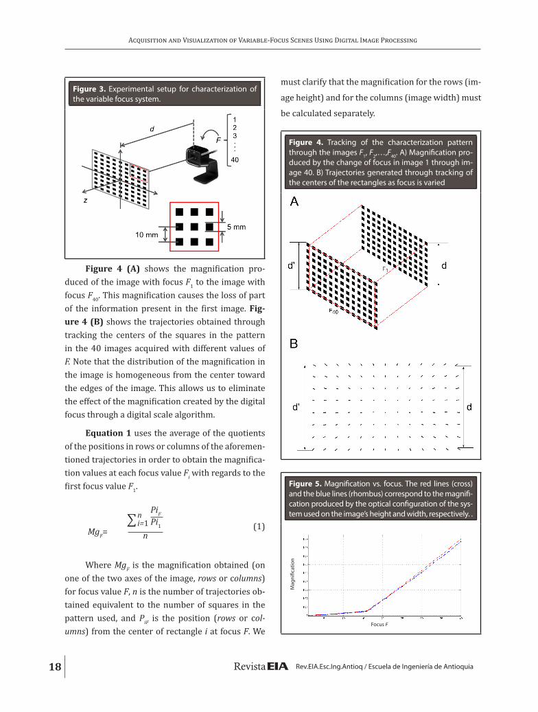
Figure 3. Experimental setup for characterization of the variable focus system.

Figure 4 (A) shows the magnification pro-duced of the image with focus F1 to the image with focus F40. This magnification causes the loss of part of the information present in the first image. Fig-ure 4 (B) shows the trajectories obtained through tracking the centers of the squares in the pattern in the 40 images acquired with different values of F. Note that the distribution of the magnification in the image is homogeneous from the center toward the edges of the image. This allows us to eliminate the effect of the magnification created by the digital focus through a digital scale algorithm.

Equation 1 uses the average of the quotients of the positions in rows or columns of the aforemen-tioned trajectories in order to obtain the magnifica-tion values at each focus value Fi with regards to the first focus value F1.

PiF�n

Pi1i=1MgF= n

(1)

Where MgF is the magnification obtained (on one of the two axes of the image, rows or columns) for focus value F, n is the number of trajectories ob-tained equivalent to the number of squares in the pattern used, and PiF is the position (rows or col-umns) from the center of rectangle i at focus F. We

must clarify that the magnification for the rows (im-

age height) and for the columns (image width) must

be calculated separately.

Figure 4. Tracking of the characterization pattern through the images F1, F2,…,F40. A) Magnification pro-duced by the change of focus in image 1 through im-age 40. B) Trajectories generated through tracking of the centers of the rectangles as focus is varied

Figure 5. Magnification vs. focus. The red lines (cross) and the blue lines (rhombus) correspond to the magnifi-cation produced by the optical configuration of the sys-tem used on the image’s height and width, respectively. .

Mag

nific

atio

n

Focus F

19



Figure 5 shows the magnification curve ob-tained for the optical system used in this project. Here we clearly see that it is a curve made up of two linear sections. The first section goes from F1 to F17 and has slow growth. The second section goes from F18 to F40 and has much greater growth in magnification.

In this case, the first section consists of the focus values corresponding to distances of 27 cm (approx.) for F17 and to an infinite distance for F1, but with a very small focus variation and a very large depth of field. Therefore, only the second group in the section (F18 to F40) is of interest for this application.

Due to the high linearity of magnification MgF in relation to the value of F in the second section of the characterization made for the optical system used (see Figure 1), it was possible to carry out a simple linear interpolation (Equation 2) using the first and final values of F and MgF obtained using Equation 1.

MF = Mgmin+ (Mgmax– Mgmin) F – Fmin

Fmax– Fmin

(2)

Where MF is the estimated magnification value for digital focus F. Mgmin and Mgmax are the magnifi-cation values obtained using Equation 1 for focus values Fmin and Fmax respectively. In this experiment, Fmin = 18 y Fmax=40.

Generally, manufacturers of optical devices with a parametric focus value ensure that the ratio between the control parameter and the magnifica-tion generated in the image is linear. However, the type of interpolation applied in the characterization of the optical system may vary according to the par-ticular characteristics of the system used.

B. Correction

The image acquisition process consists of tak-ing n images with different values of F while keeping the scene still and maintaining the spatial configura-tion of the camera mount. For each image, the value of F is known.

As was mentioned above, this variable focus ac-quisition process creates a magnification (Figure 5) which must be corrected so that it is not seen in the subsequent process of calculating the focus map. Giv-en that the size of the image is maintained, it is clear that there will be areas in the image without magni-fication (F18) that do not appear in the images at (F19 ,..., F40). Therefore, the greatest amount of recoverable information about the scene will be that which ap-pears in the image at F40. Therefore, the correction process has two stages. The first consists of changing the size of the image depending on its magnification factor, and the second consists of trimming the image so that only the information present in image F40 ap-pears. From the above, it is clear that the change in size consists of taking any image between F18 ,..., F39 to the magnification generated at F40 , which is pos-sible when we calculate the inverse value of the mag-nification of the image that we wish to correct since the behavior of the magnification is linear. Therefore, the correction factor for the magnification of the im-age would be described by Equation 3.

CMF=0.034(58 – F) + 0.9386; F = {18,…,39} (3)

If δ(I, k) is a function that magnifies image I by a factor k then the first stage of the image correction would be described by Equation 4.

IRF= δ(IF ,CMF); F={18,…,39} (4)

Where IRF is the corrected image in the first stage and, IF is the image that corresponds to digital focus F.

The second stage of correction consists of trimming the portion of the images F18 ,..., F39 that is not visible in the image with the greatest magnifica-tion F40. This process consists of trimming the bor-ders of said images such that their final dimensions are equal to the camera resolution.

If sV and sH are the number of the camera’s vertical and horizontal pixels, and ε(I, dH, dV, sH, sV) is a function that returns a portion of image I with resolution (m, n), equivalent to a rectangle situated at point (dV, dH) and with the horizontal and vertical

20



increase of sV, sH respectively, (see Figure 6); dV, dH will be defined by Equations 5 and 6.

dV= ⌊ 0.5 * |m–sV| ⌋ (5)

dH= ⌊ 0.5 * |n–sH| ⌋ (6)

Figure 6. Parameters for the trimming stage.

C. Focus map calculation

The goal of the focus map calculation is to de-termine the value of F that achieves the greatest value for each pixel in the image. To do so, we need a focus metric that allows us to numerically measure how focused a particular pixel is. In this project, the “sum of modified Laplacian” (Nayar & Nakgawa, 1994) was used as a focus/blur operator due to its robustness in responding to high-frequency varia-tions in the image (edges or high-contrast regions) and the simplicity of its implementation, which does not imply that other operators can be used in future implementations. This operator is defined by Equa-tions 7 and 8.

ML(x, y) = |2*IR(x, y) – IR(x – paso, y) – IR(x + paso, y)| + |2 * IR(x, y) – IR(x, y – paso) – IR(x, y + paso)|

(7)

i+N j+NGF (i, j)= � � ML(x, y)

x=i–N y=j–N(8)

Where ML(x, y) is the modified Laplacian oper-ator for the pixel at position x, y, and paso is a value that allow us to “skip” the closest near neighbor in said proportion. GF (i, j) is a function that returns the value of the amount of the modified Laplacian for a pixel at position i, j using a window of N × N near neighbors for the image that corresponds to digital focus F.

Using Equations 7 and 8, the focus map cal-culation process consists of finding the F with the greatest value for each pixel in the acquired images, equivalent to the greatest focus (Equation 9).

MF(i, j) = argmax(GF (i, j)); F = {18,…,40} (9)

Finally, a bilateral filter proposed in (Tomasi & Manduchi, 1998) is applied to avoid effects pro-duced by noise in the acquisition system.

MF(i, j) = BF(MF, k, σ) (10)

Where BF(MF, k, σ) is a function that returns the output image after applying the bilateral filter on the input image MF using a local neighborhood size k and a standard deviation σ. MF must be a floating image within the range [0,1].

D. Selection of the image

This stage consists of visualizing the image that presents the greatest focus in a region selected by the user through a graphic interface.

If SF(i,j,k) is a function that returns the average of F in a region defined by a square kernel from side k and centered on the pixel at position i, j, then:

�� x=i+t � y=j+t ML(x, y)

�x=i–t y=j–t

SF (i,j,k) = ;t=k\2 (11)k2

The goal of using a kernel in the previous cal-culation lies in using focus information near the pixel in which we are interested based on the sup-position that nearby pixels must present a similar level of focus. This minimizes the effect of artifacts generated in the previous processes in calculating the value of F.

21



Finally, visualization of the focused image con-sists of displaying the corrected image which corre-sponds to the value SF.

E. Obtaining a completely focused image

A refocused image IFa can be calculated using the average of the images calculated at the different focuses (Levoy, 2006) (Equation 12).

�40 IRFF=18IFa = ; n = 18 – 40 (12)

n

Where IRF to the corrected image at focus F. However, the resulting image shows a blur effect due to the fact that for each area of the image, we only have one image in which it shows maximum focus.

Using the focus map MF previously calculated, it is possible to obtain an image IFb in which all of the pixels appear with maximum focus (Equation 13).

IFb(i) = IRF (i); i = (MF== F) (13)

Where i is a vector R2 of positions with value F on the focus map MF, that is, a vector of positions of pixels that show a maximum value for focus F. How-ever, this image shows noise produced by the local nature of the focus operator.

In this paper, we propose the combination of the above equations to achieve an image with com-plete focus IFc that presents a high level of contrast and a low level of noise (Equation 14).

IFc =IFa+ IFb

2(14)

3. RESULTS AND DISCUSSION

We performed an experiment to validate the viability of using the proposed method on simple and complex scenes, as well as to determine the con-ditions necessary for its correct implementation.

For the experiment, acquisitions were per-formed for scenes with conditions that represent possible application cases. The algorithms were implemented without any kind of optimization or parallelization of code given that the goal of the ex-periment was not to determine the method’s com-putational complexity.

Figure 7 shows the result of the proposed method applied to two scenes. The first is a scene with high contrast in laboratory conditions, and the second is a natural scene that shows areas with high and low contrast. In group A, we can see the focus map obtained by Equation 10. Note that the low-contrast regions in scene 2 (clouds, building wall) generate areas of confusion on the focus map due to the fact that the focus operator returns a similar value for each of the images at different values of F. However, in scene 1, the focus map corresponds pre-cisely to the scene’s real focus information given the high contrast generated by the printed text. Nayar et al. (1996) propose using a white light pattern over the scene in order to improve the contrast and thereby the precision of the focus operator. How-ever, this is not a viable option for natural scenes since the light pattern must be projected with a high lumen value on scenes with a great deal of illumina-tion or because this pattern alters the original im-age. A possible option for handling this limitation in a commercial system would be to automatically es-timate a given number of focus points that the user can select, that is, points with a high local contrast.

Groups B, C, and D correspond to the selection of the image determined by Equation 11 for areas with different focuses, from the furthest to the near-est, respectively, using a graphic user interface to se-lect the points in the scene on which the user wishes to focus (blue line).

Figure 8 shows the result of obtaining a com-pletely focused image for the two scenes in Figure 7, which are the results of using the image average technique (A), the focus map technique (B), and the combination of the two (C). Note that group (A)

22



shows a high level of blur; group (B) shows greater contrast but also noise generated by the local nature of obtaining the focus map; group (C) shows the av-erage of both images (A and B), achieving a pleasing visual appearance with a lower level of contrast than that obtained in (B) but with a lower level of noise.

An important limitation of this project is the impossibility of acquiring scenes in motion due to the fact that the images for each focus are taken at different moments, which implies that the scene will be modified over time and, therefore, the calculated focus map will not be absolute.

Figure 9 shows what was discussed above. Note that given the movement of the second hand of

Figure 7. Test scene with multi-focus information. (A, B, C, D) Images selected with the proposed algorithm with focuses of greater distance in A to lesser distance in D with respect to the camera.

the watch in the scene, artifacts are produced in the completely focused image (C).

Technologies such as liquid lenses (Oku & Ishikawa, 2010) and MEMS cameras (Wei et al., 2012) that allow approximate focus speeds of 10 ms allow us to confront this limitation. In addition, given that the focus map is related to the scene’s fo-cus value, by performing a prior calibration of the focus vs. distance value, it would be possible to use the proposed method to calculate the map of the scene’s range for tridimensional reconstruction ap-plications in real time, such as tridimensional mi-croscopy and robotic navigation.

23



Figure 9. Scene in motion. (A), (B) scenes with distant and close focus, respectively. (C) noise produced by the move-ment of the watch’s second hand in the different acquisitions of the scene..

Figure 8. Scenes with complete focus. (A) According to equation 12, (B) According to equation 13, (C) According to equation 14.

24



4. CONCLUSIONS

This paper presented a method for acquiring and visualizing images of scenes with multiple fo-cuses. The method’s implementation is simple, al-lowing it to be used in scenes without controlled conditions, which is of interest for its implementa-tion in mobile phones or personal cameras.

This method considers the acquisition sys-tem’s initial characteristics, which allows for its im-plementation in systems with optical configurations that differ from those used in this experiment.

Since the method requires a focus operator, and since the focus operator, in turn, works with local contrast measurements, we can obtain unde-sired results in the focus map of the regions in the scene with low contrast. However, this depends to a large degree on the resolution of the camera’s sen-sor since the greater the resolution, the greater the level of detail and, therefore, the greater the level of contrast in the objects in the scene.

For future work, we propose extending this method to obtain a map of the depth of the acquired scene and implementing rapid focus systems such as liquid lenses for its application in scenes in motion.

REFERENCESAdelson, E. H.; Wang, J. (1992). Single Lens Stereo with

a Plenoptic Camera. IEEE Transaction on Pattern Analysis and Machine Intelligence, 14(2), February, pp. 96-106.

Bai, X. et al. (2015). Quadtree-Based Multi-Focus Image Fusion Using a Weighted Focus-Measure. Informa-tion Fusion, 22, March, pp. 105–118.

Chen, L., Li, J.; Philip-Chen, C.L. (2013). Regional Multifo-cus Image Fusion Using Sparse Representation. Op-tics Express, 21(4), pp. 5182-5197.

De, I.; Chanda, B. (2015). Multi-Focus Image Fusion Us-ing a Morphology-Based Focus Measure in a Quad-Tree Structure. Information Fusion, 14(2), April, pp.136–146.

Favaro, P.; Soatto, S. (2007). 3-D Shape Estimation and Image Restoration: Exploiting Defocus and Motion-Blur. Springer-Verlag London.

Huang, W.; Jing, Z. (2007). Evaluation of Focus Measures in Multi-Focus Image Fusion. Pattern Recognition Let-ters, 28(4), March, pp. 493-500.

Levoy, M. (2006). Light Fields and Computational Imag-ing. Computer, IEEE Computer Society, 39(8), Au-gust, pp. 46–55.

Li, S. et al. (2013). Image Matting for Fusion of Multi-Fo-cus Images in Dynamic Scenes. Information Fusion, 14(2), April, pp. 147-162.

Li, S., Kwok, J. T.; Wang, Y. (2002). Multifocus Image Fusion Using Artificial Neural Networks. Pattern Recogni-tion Letters, 23(8), June, pp. 985–997.

Liu, C. et al. (2015). Multi-Focus Image Fusion Based on Spatial Frequency in Discrete Cosine Transform Do-main. Signal Processing Letters, 22(2), February, pp. 220–224.

Liu, Z. et al. (2001). Image Fusion by Using Steerable Pyra-mid. Pattern Recognition Letters, 22(9), July, pp. 929–939.

Lorenzo, J. et al. (2008). Exploring the Use of Local Binary Patterns as Focus Measure. In Computational Intel-ligence for Modelling Control & Automation, 2008 International Conference on. Vienna, 10-12 Decem-ber.

Nayar, S.K.; Nakgawa, Y. (1994). Shape From Focus. Pat-tern Analysis and Machine Intelligence, IEEE Trans-actions on, 16(8), August, pp. 824–831.

Nayar, S.K., Watanabe, M.; Noguchi, M. (1996). Real-Time Focus Range Sensor. IEEE Transactions on Pattern Analysis and Machine Intelligence, 18 (12), Decem-ber, pp. 1186-1198.

Nejati, M., Samavi, S. Y Shirani, S. (2015). Multi-Focus Im-age Fusion Using Dictionary-Based Sparse Repre-sentation. Information Fusion, 25, pp. 72–84.

Oku, H.; Ishikawa, M. (2010). High-Speed Liquid Lens for Computer Vision. In Robotics and Automation (ICRA), IEEE International Conference on. Anchor-age, AK, 3-7 May.

Richter, J.P. (1970). The Notebooks of Leonardo Da Vinci. 2nd ed. Dover Publications. 514 p.

Saeed, A.; Choi, T.-S. (2008). A Novel Algorithm for Esti-mation of Depth ap Using Image Focus for 3D Shape Recovery in the Presence of Noise. Pattern Recogni-tion, 41(7), pp. 2200–2225.

25



Saeedi, J.; Faez, K. (2009). Fisher Classifier and Fuzzy Log-ic Based Multi-Focus Image Fusion. In Intelligent Computing and Intelligent Systems, 2009. ICIS 2009. IEEE International Conference on, 4, pp. 420–425.

Santhosh, J., et al. (2014). Application of SiDWT with ex-tended PCA for multi-focus images. In Medical Im-aging, m-Health and Emerging Communication Sys-tems (MedCom), 2014 International Conference on, November, pp. 55–59.

Song, Y. et al. (2006). A New Wavelet Based Multi-focus Image Fusion Scheme and Its Application on Optical Microscopy. In Robotics and Biomimetics, 2006. RO-BIO ’06. IEEE International Conference on, Decem-ber, pp. 401–405.

Subbarao, M., Chor, T.-S.; Nikzad, A. (1993). Focusing Tech-niques. Optical Engineering, 32(11), November, pp. 2824-2836.

Tomasi, C.; Manduchi, R. (1998). Bilateral Filtering for Gray and Color Images. In Computer Vision, 1998. Sixth In-ternational Conference on. January, pp. 839–846.

Wan, T., Zhu, C.; Qin, Z. (2013). Multifocus Image Fusion Based on Robust Principal Component Analysis. Pat-tern Recognition Letters, 34(9), July, pp. 1001–1008.

Wang, X., Wei, Y.-L.; Liu, F. (2013). A New Multi-Source Image Sequence Fusion Algorithm Based on SIDWT. In ICIG ’13 Proceedings of the 2013 Seventh International Con-ference on Image and Graphics, pp. 568–571.

Wei, H. et al. (2012). Controlling a MEMS Deformable Mir-ror in a Miniature Auto-Focusing Imaging System. Control Systems Technology, IEEE Transactions on, 20 (6), pp. 1592–1596.

Yang, B.; Li, S. (2012). Pixel-Level Image Fusion with Si-multaneous Orthogonal Matching Pursuit. Informa-tion Fusion, 13(1), January, pp. 10–19.

Zygmunt, P. (2001). Perception Viewed as an Inverse Problem. Vision Research, 41(24), November, pp. 3145 – 3161.

TO REFERENCE THIS ARTICLE /PARA CITAR ESTE ARTÍCULO /

PARA CITAR ESTE ARTIGO /

Atencio-Ortiz, P.; Arias-Gallego, A.; Arias-Correa, M. (2015). Acquisition and Visualization of Variable-Focus Scenes Us-ing Digital Image Processing. Revista EIA, 12(24), July-De-cember, pp. 13-25. [Online]. Available on: DOI: http:/dx.doi.org/10.14508/reia.2015.12.24.13-25

ACQUISITION AND VISUALIZATION OF VARIABLE- FOCUS …

Documents

Transcript of ACQUISITION AND VISUALIZATION OF VARIABLE- FOCUS …