Accurate, Low-Energy Trajectory Mapping for Mobile Devices

Arvind Thiagarajan, Lenin Ravindranath, Hari Balakrishnan, Samuel Madden, Lewis GirodMIT Computer Science and Artificial Intelligence Laboratory

{arvindt, lenin, hari, madden, girod}@csail.mit.edu

AbstractCTrack is an energy-efficient system for trajectory map-ping using raw position tracks obtained largely fromcellular base station fingerprints. Trajectory mapping,which involves taking a sequence of raw position sam-ples and producing the most likely path followed bythe user, is an important component in many location-based services including crowd-sourced traffic monitor-ing, navigation and routing, and personalized trip man-agement. Using only cellular (GSM) fingerprints insteadof power-hungry GPS and WiFi radios, the marginal en-ergy consumed for trajectory mapping is zero. This ap-proach is non-trivial because we need to process streamsof highly inaccurate GSM localization samples (aver-age error of over 175 meters) and produce an accuratetrajectory. CTrack meets this challenge using a noveltwo-pass Hidden Markov Model that sequences cellu-lar GSM fingerprints directly without converting them togeographic coordinates, and fuses data from low-energysensors available on most commodity smart-phones, in-cluding accelerometers (to detect movement) and mag-netic compasses (to detect turns). We have implementedCTrack on the Android platform, and evaluated it on 126hours (1,074 miles) of real driving traces in an urban en-vironment. We find that CTrack can retrieve over 75%of a user’s drive accurately in the median. An impor-tant by-product of CTrack is that even devices with noGPS or WiFi (constituting a significant fraction of to-day’s phones) can contribute and benefit from accurateposition data.

1 INTRODUCTION

With the proliferation of sensor-equipped smartphones,the decades-long promise of location-based mobile ser-vices and mobile sensing applications is finally becom-ing real. Many location-based applications periodicallyprobe the device’s position sensor to obtain a stream ofposition samples, and then process this stream to ob-tain a trajectory. Examples include crowd-sourced traf-fic and navigation applications [15, 33], personalizedtrip management applications [28, 15], fleet manage-ment applications [21], and mobile object/asset track-ing [11, 34, 7, 19, 25]. The fundamental problem in theseapplications is trajectory mapping, where the goal is to

produce the most likely trajectory—a sequence of mapsegments—traversed by the mobile device.

If each device could always use a GPS sensor, thisproblem is straightforward because the majority of theposition samples would usually be accurate to within asmall number of meters. For applications that require po-sitions to be monitored continuously, however, GPS hassome significant practical limitations. First, GPS chipsetson today’s mobile devices consume a non-trivial amountof energy, causing a significant reduction in battery life(§2). Second, in many embedded tracking applications,objects are packaged deep inside vehicles and do nothave a clear line-of-sight to GPS satellites e.g., anti-theftsystems on vehicles (often hidden under layers of metal),systems that track couriered packages [11] and systemslike TrashTrack [34] for tracking waste and recycled ma-terials. Most of these tracking applications also face en-ergy and cost constraints. Third, antenna limitations oncommodity mobile devices cause poor GPS performancein “urban canyons” and near high-rise buildings. Finally,a large number of phones today simply do not have GPSon them—85% of phones shipped in 2009, and projectedto be over 50% for the next five years [6]. The users ofthese devices, a disproportionate number of whom are indeveloping regions, are largely being left out of the manynew location-based applications.

This paper describes the design, implementation, andexperimental evaluation of CTrack, a system for map-ping the trajectory of mobile devices without using GPS.The noteworthy aspect of CTrack is that it uses muchless energy than current approaches, which use GPS,WiFi localization [32, 8], or a combination of the two.CTrack processes a stream of raw, highly inaccurate po-sition samples from mobile devices obtained by finger-printing cellular GSM base stations, and matches themto segments on a known map in a way that achieves highaccuracy. The marginal energy cost of gathering a fin-gerprint (a list of nearby GSM towers and their signalstrengths) is zero on mobile phones because the cellu-lar radio is usually always on. CTrack optionally aug-ments GSM fingerprints with data from one or more of aphone’s accelerometer, compass, and gyro, all of whichconsume tiny amounts of energy, using these sensor hints

1

Figure 1: GSM Localization Errors. Raw location sam-ples are in red and the true driving path is in black.

to identify the kind of movement and improve the accu-racy of trajectory mapping.

GSM localization using, for example, the Placelab [8]approach, leads to errors of 100–200 meters in dense ur-ban areas, and as much as 1 km in some areas. Such er-rors are too large for many applications, which requireresults with sufficient accuracy to pinpoint a specific roadsegment or route driven by a user. Figure 1 illustrates theproblem with existing GSM localization. The red pointsare raw locations obtained from our implementation ofcellular positioning as used in Placelab [8]. The actualroads traversed (ground truth) are shown in black. Di-rectly reporting raw positions or matching locations tothe nearest segments in the road map would result in un-acceptably low accuracy for the applications mentionedat the beginning of this section.

CTrack makes it possible to use GSM fingerprints foraccurate trajectory mapping using two novel ideas. Likeprevious approaches e.g. VTrack [32], CTrack matches asequence of GSM tower observations, rather than a sin-gle point at a time, using constraints on the transitions amoving vehicle can make between locations. However,unlike VTrack, which first converts radio fingerprints to(lat, lon) coordinates, CTrack matches cellular finger-prints directly to a map without first converting theminto (lat, lon) coordinates, an insight critical to achiev-ing high accuracy. Instead, CTrack uses a two-pass algo-rithm. The first pass is a Hidden Markov Model (HMM)that divides space into grid cells, and determines the mostlikely sequence of traversed grid cells. The second passuses a different HMM to match the traversed grid cellsequence to road segments.

The second idea in CTrack is to (optionally) fuse in-formation from two low-energy phone sensors: the ac-celerometer and a compass or gyroscope. CTrack usesthe compass/gyro to detect if the driving path took a turn,and the accelerometer to determine if the user is stoppedor moving. These sensor hints can correct some commonsystematic errors that arise in GSM localization.

We implemented CTrack on the Android smartphoneplatform, and evaluated it on nearly 125 hours of real

drives (1,074 total miles) from 20 Android phones in theBoston area. We find that:

1. CTrack is good at identifying the sequence of roadsegments driven by a user, achieving 75% precision and80% recall accuracy. This is significantly better thanstate-of-the-art cellular fingerprinting approaches [8] ap-plied to the same data, reducing the error of trajectorymatches by a factor of 2.5×.

2. Although CTrack identifies the exact segment oftravel incorrectly 25% of the time, trajectories producedby CTrack are on average only 45 meters away fromthe true trajectory. This implies that our system is usefulfor applications like route visualization. In this respect,CTrack is 3.5× better than map-matching raw cellularfingerprints, which results in 156 meters median error.

3. CTrack has a significantly better energy-accuracytrade-off than sub-sampling GPS data to save energy, re-ducing energy cost by a factor of 2.5× for the same levelof accuracy.

2 WHY CELLULAR?One of the key motivations for CTrack is that it uses sub-stantially less energy than GPS. This is to be expectedfrom a theoretical standpoint because of the differencein effective radiated power (ERP) for the two systems.GPS satellites fly in an orbit 11,000 miles above theearth, with a transmission power of 50 W, resulting in2×10−11 mW/m2 at the receiver; in contrast, typical cel-lular systems register an ERP of up to 10 mW/m2 [14].This difference of 117 dB translates directly into energyconsumption at the receiver, as the difference must becompensated by additional processing gain and amplifi-cation. The ERP difference also explains why GPS sig-nals cannot be acquired without relatively unobstructedline-of-sight to orbiting satellites, and why they are moresensitive to weather conditions than GSM signals.

2.1 Energy MeasurementsWe performed a simple experiment to quantify the en-ergy consumption of each of the sensors of interest —GPS, WiFi, GSM, the compass and the accelerometer onan Android G1 phone. For each sensor, we wrote an An-droid application to continuously sample the sensor atsome given frequency, as well as continuously query thebattery level indicator. We charged the phone to 100%,configured the screen to turn off automatically when idle(the default), and started the application. We used the An-droid telephony API to retrieve nearby cell towers andtheir associated signal strength values.

Figure 2 shows the reported battery life as a functionof time for four configurations: GPS sampled every sec-ond, GPS sub-sampled every two minutes, WiFi scannedevery second, and the configuration used by CTrack —scanning GSM cell towers every second, and the com-

2

0

20

40

60

80

100

0 500 1000 1500 2000 2500 3000 3500

Rem

aini

ng B

atte

ry L

ife (

perc

enta

ge)

Time Elapsed (minutes)

CTrack: GSM @1Hz + Compass,Accl@20HzGPS every 1s

GPS every 120sWiFi every 1s

Figure 2: Energy Consumption: GPS vs WiFi vs CTrackon an Android Phone.

pass and accelerometer at 20 Hz. CTrack results in asaving of approximately 10× in battery life compared toGPS every second over 6× compared to WiFi every sec-ond. Also, although sub-sampling GPS ever 2 minutessaves energy over continuously sampling it, we showlater that sub-sampling also hurts accuracy. The batterydrain curves look irregular because the G1 phone esti-mates remaining battery life poorly – the same experi-ment on a Nexus One (a later model) showed a similartrend, but looked like a straight line for all sensors.

2.2 Other Energy Studies and DiscussionThe numbers above are consistent many previous stud-ies conducted on a range of phones. For example, wefound [32, 31] that continuously sampling GPS oniPhone 3G and 4 resulted in 3–10 hours total battery life(iPhone 3G has lower battery life, and screen brightnessvaried in the different papers, resulting in different runtimes even without GPS). Leaving the phone on (withscreen on) resulted in 10–18 hours of lifetime (this wouldbe higher if we could turn the phone’s screen off, but atthe time, non-jailbroken iPhones did not support back-ground applications.)

In [23], the authors showed that Nokia N95 phonesuse about 370 mW of power when GPS is left on, versus60 mW when idling, and that continuous (once a second)GPS sampling results in 9 hours of total battery life. Sev-eral other papers [36, 16, 5, 9, 13] suggest similar num-bers for N95 phones (battery life in the 7–11 hour range)with regular GPS sampling. On a more recent AT&T Tiltphone [18], the authors found that continuous GPS sam-pling used 400 mW, a single GPS fix costs 1.4-5.7 J ofenergy (depending on whether previous seen satellite in-formation is cached or not) and a WiFi scan consumedabout 0.55 J of energy.

The energy cost of GPS is rooted in the need for pro-cessing gain to acquire the positioning signals. As signalquality degrades due to obstructions or weather condi-tions, the energy cost of recovering the signal increases.In contrast, because phones continuously track cell tow-

ers as a part of normal operation, the marginal energycost of CTrack is driven by CPU load. Processing a celltower signature might require at most 100,000 instruc-tions, which costs 5 nJ on a current generation 1 GHzQualcomm Snapdragon processor.

In embedded (non-phone) applications that don’t needthe radio on, it is possible to track only the signal qual-ity and cell ID portions of the GSM protocol. This re-quires observing only the BCH slots of the GSM beaconchannel, which are 4.6 ms long and are transmitted onceper each 1.8 second cycle. A 10% GSM receiver dutycycle should be adequate to track the strongest towers.Assuming a GSM receiver uses 17 mA at 100% duty cy-cle, this represents an additional power consumption of 5mW (1.7 mA @ 2.7 V)amortized cost assuming 17 mAcost for receiver circuitry [1, 30].

Accelerometers and compasses (magnetometers) alsohave low overhead—for example ADXL 330 accelerom-eters use about 0.6 mW when continuously sampling,and at 10 Hz can be idle about 90% of the time, suggest-ing a power overhead of around .06 mW for sampling theaccelerometer [2]. The MicroMag3 compass uses about1.5 mW in continuous sampling, suggesting a power con-sumption of .15 mW or less at 10 Hz [24].

In summary, the power consumption of cellular scan-ning plus sensors on phones is less than 5 mW, and thepower consumption of sensors alone if cellular is free—as is typical—is less than 1 mW, low enough that it doesnot reduce the phone’s overall lifetime even when instandby mode, when it consumes 20–30 mW of power.In contrast, the best case for GPS is 75 mW in trackingmode when a fix is already acquired, but in practice iscloser to 400 mW when including the energy to periodi-cally re-acquire fixes, and is similar for WiFi scans everysecond or two. The power differential is thus significant.

2.3 Embedded Low-Power ApplicationsCTrack can also be applied outside the smartphone con-text to embedded low-power tagging applications. Forthese applications, minimizing cost and battery require-ments is essential. These applications benefit from usingGSM in place of GPS because of increased flexibility ofantenna placement for cellular systems, and resilience toobstructed environments.

One such application is cold-chain management wherethe focus is on monitoring the temperature of a pack-age during its shipping. A low-power passive cellular re-ceiver can be used to record cellular fingerprints duringtransport. Upon arrival, CTrack can be run on the fin-gerprints to compute the shipment’s trajectory and maptemperature readings on to it.

Another embedded application of CTrack is Trash-Track [34, 7], where items of trash were tagged withactive tags that traced the items through the path along

3

GSM Scanning Accel. Compass

DifferentialCompression

Sensor Hint Extraction

Cell Towers PhoneApplication

CellularFingerprints

CTrack Phone Library

Turn, MovementHints

ServerDatabase

Trajectory MappingAlgorithm

MatchingResults

Filters (e.g, Driving)

On Server

CTrack Web Service

CentralServer

On Phone

Batch Transmission

Over Network

Queries

Figure 3: CTrack System Architecture.

the “disposal chain”. Because the tag will eventually bedestroyed, this system needs cellular communication ca-pabilities; using the same technology for trajectory map-ping consumes lower power, has lower cost, and is morerobust than adding a GPS receiver to the tag.

3 SYSTEM OVERVIEW

We now describe the design of CTrack. Figure 3 showsthe system architecture. It consists of two software com-ponents, the CTrack Phone Library, and the CTrack WebService. The library collects, filters, and scans for GSMand sensor data on the phones, and transmits it via anyavailable wireless network (3G, WiFi, etc.) to the webservice, which runs the trajectory mapping algorithmon batches of sensor data to produce map-matched tra-jectories. The mapping algorithm runs on the server toavoid storing complete copies of map data on the mobiledevice, and to provide a centralized database to whichphone or web applications can connect to view and an-alyze matched tracks (e.g., for visualizing road traffic orthe path taken by a package or vehicle).

Phone Library: The phone library collects a list of GSMtowers and optionally, if accelerometer, compass, or gyroare available on the phone, current sensor hints. Thesesensor hints are binary values indicating if the phoneis moving and/or turning; Section 5 describes how weextract sensor hints. The phone library also filters ac-celerometer data to detect if the user is stationary orwalking (as in [27, 31]), for applications that want dataonly from moving vehicles. The library may also be con-figured to periodically collect GPS data for use in thetraining phase of our algorithm from users who wish tocontribute.

Our implementation collects about 120 bytes/second

of raw ASCII data on average. This quantity varies be-cause the number of cell towers visible varies with lo-cation. We use simple gzip compression, which on ourtest drives resulted in just 11 bytes/second of data to bedelivered. We batch this data and upload a batch every tseconds. At 11 bytes/sec, with even small batches, usinga 3G uplink with an upload speed of 30 kBytes/s (typicalof most current 3G networks in the US) results in verylow 3G radio duty cycles—for example, setting t to 60seconds results in the radio being awake only 0.03% ofthe time, which consumes a negligible amount of addi-tional power. Once-per-minute (t = 60) reporting is suf-ficient for most applications we are concerned with, in-cluding traffic reporting, package tracking, and vehiculartheft detection.

We chose not to run trajectory matching on the phonebecause it results in a negligible space savings, whileconsuming extra CPU overhead and energy. For low datarates, the primary determinant of 3G or WiFi transmis-sion energy is the transmitter duty cycle [4], makingbatch reports a good idea. However, we do extract sen-sor hints on the phone because the algorithms for hintextraction are simple and add negligible CPU overhead,while significantly reducing data rate. The raw data ratefrom sampling the accelerometer/compass without com-pression or hint extraction is about 1.3 MBytes/hour,which means that an application collecting this data froma user’s phone for two hours a day could easily rack up asubstantial bandwidth bill without on-phone filtering.

CTrack Web Service: The web service receives GSMfingerprints and converts them into map-matched tra-jectories using the trajectory mapping algorithm. Thesematched trajectories are written into a database. Option-ally, the user’s current segment can be sent directly backto the phone. A detailed description of the trajectorymapping algorithm is given in the next section.

4 TRAJECTORY MAPPING ALGORITHM

CTrack’s algorithm for map-matching a sequence ofGSM cell tower observations (“cellular fingerprints”)differs from previous approaches in two key ways. First,we do not convert cellular fingerprints into (lat, lon) co-ordinates before matching them to segments. We findthat reducing a fingerprint to a single geographic loca-tion loses a lot of information because a given cellularfingerprint is often seen from multiple locations quite farapart. This situation is unlike the WiFi map-matching inVTrack [32], where this spread is small, and the approachof converting to centroids worked well. Second, CTrackoptionally fuses sensor hints from the accelerometer andthe compass to improve matching accuracy. We showthat turn hints can help remove spurious turns and kinksfrom GSM-mapped trajectories, and movement hints can

4

Grid Sequencing

Road Map

War-drivingDatabase

Smoothing andInterpolation

Segment Matching

Input DriveCell Tower

FingerprintsSensor Hints

Sequence of Grids

Sequence of Road Segments

Sequence of Coordinates

Figure 4: Trajectory Mapping Algorithm.

help remove loops, a common problem with GSM local-ization when a vehicle is stationary.

4.1 Algorithm OutlineThe goal of the algorithm is to associate a sequence ofcellular fingerprints to a sequence of road segments on aknown map. Our algorithm takes as input:

1. A series of GSM fingerprints from the phone, oneper second in our implementation. In our paper, theterm GSM fingerprint refers to a set of observed IDs ofcell towers and their associated received signal strength(RSSI) values. In our implementation, the Android OSgives us the cell ID and the RSSI of up to 6 neighbor-ing towers in addition to the associated cell tower. EachRSSI value is an integer on a scale from 0 to 31 (highermeans higher signal-to-noise ratio).

2. If available, time series signals from accelerome-ter, compass, and gyroscope sampled at 20 Hz or higher.These are converted to “sensor hints” using on-phoneprocessing as explained below.

3. A known map database that contains the geogra-phy of all road segments in the area of interest, such asOpenStreetMaps [22], NAVTEQ, or TeleAtlas.

The output is the likely sequence of road segments tra-versed, one for each time instant in the input.

Figure 4 shows the components of the algorithm.Training builds a training database, which maps groundtruth locations from GPS to observed cell towers andtheir RSSI values. Grid Sequencing uses a HiddenMarkov Model (HMM) to determine a sequence of spa-tial grid cells corresponding to an input sequence ofGSM fingerprints. The output of grid sequencing issmoothed, interpolated, and fed to Segment Matching,which matches grid cells to a road map using a differ-ent HMM.

Figure 5 illustrates our algorithm by example. The in-put “raw points” in Figure 5(a) are shown only to illus-trate the extent of noise in the input data. They are not ac-tually used by CTrack. They are computed by using thePlacelab fingerprinting algorithm [8], where a cell tower

fingerprint is assigned a location equal to the centroidof the closest k fingerprints in the training database (weused k = 4).

Next, we describe each stage of the algorithm.

4.2 TrainingWe divide the geographic area of interest into uniformsquare grid cells of fixed size gs. We associate with eachcell an ordered pair of positive integers (x,y), where(0,0) represents the south-west corner of the area of in-terest. We use gs = 125 meters, chosen to balance run-ning time, which increases with smaller grid size, againstaccuracy.

We train CTrack for the area of interest using softwareon mobile phones that logs a timestamped sequence ofground truth GPS locations and associated cell tower fin-gerprints. For each grid G in the road map, our trainingdatabase stores FG, the set of distinct fingerprints seenfrom G. Training can be done out-of-band using an ap-proach similar to the Skyhook [29] fleet. Once the train-ing database is built, it can be used to map-match ortrack any drive, and needs to be updated relatively in-frequently. We can also collect new training data in-bandfrom consenting participating phones that use the CTrackweb service whenever the user has enabled GPS.

4.3 Grid SequencingGrid sequencing uses a Hidden Markov Model (HMM)to determine the sequence of grid cells correspondingto a timestamped sequence of cellular fingerprints. AnHMM is a discrete-time Markov process with a set ofhidden states and observables. Each state emits an ob-servable, whose likelihood is given by an emission score.An HMM also permits transitions among its hiddenstates at each time step. These transitions are governedby a different set of likelihoods called transition scores.

In our (first) HMM, the hidden states are grid cellsand the observables are GSM fingerprints. The emissionscore, E(G,F) captures the likelihood of observing fin-gerprint F in cell G. The transition score, T (G1,G2), cap-tures the likelihood of transitioning from cell G1 to G2 ina single time step.

We first process the input GSM fingerprints usingthe windowing technique described below. We then useViterbi decoding [35] to find the maximum likelihoodsequence of grid cells corresponding to the windowedversion of the input sequence. The maximum likelihoodsequence is defined to be the sequence that maximizesthe product of emission and transition scores.

We now describe the four parts of this HMM: window-ing, hidden states, emission score, and transition score.Windowing. Because it is common for a single celltower scan to miss some of the towers near the currentlocation, we group the fingerprints into windows ratherthan use the raw fingerprints captured once per second.

5

(a) Raw points before sequencing

(b) After Grid Sequencing

(c) After smoothing

(d) Final map-matched output

Figure 5: CTrack map-matching pipeline. Black lines areground truth and red points/lines are obtained from cel-lular fingerprints.

We aggregate the fingerprints seen over Wscan secondsof scanning. We chose Wscan = 5 seconds empirically:the phone typically sees all nearby cell towers within 3scans, which takes about 5 seconds. In our evaluation, weshow that windowing improves accuracy (Table 1).Hidden States. The hidden states of our HMM are gridcells. Given an observed fingerprint F , a grid cell G is acandidate hidden state for F if there is at least one train-ing fingerprint in G that has at least one cell tower incommon with F . Note that we might sometimes omit avalid possible hidden state G if the training data for G issparse. To overcome this problem, we use a simple wire-less propagation model to predict the set of cell towersseen from cells that contain no training data. The modelcomputes the centroid and diameter of the set of all ge-ographic locations from which each cell tower is seen inthe training data. The model draws a “virtual circle” withthis center and diameter and assumes that all cells in thecircle see the tower in question.Emission Score. Our emission score E(F,G) is intendedto be proportional to the likelihood that a fingerprint F isobserved from grid cell G. A larger emission score meansthat a cell is a more likely match for the observed finger-print. Our emission score uses the following heuristic.We find Fc, the closest fingerprint to F seen in trainingdata for G. “Closest” is defined to be the value of Fc thatmaximizes a pairwise emission score EP(F,Fc). Our pair-wise score is inspired by RADAR [3]. It captures boththe number of matching cell IDs, M, between two fin-gerprints, and the Euclidean distance dR in between thesignal strength vectors of the matching towers:

EP(F1,F2) = Mλmatch +(dmaxR −dR(F1,F2)) (1)

where λmatch is a weighting parameter and dmaxR = 32 is

the maximum possible RSSI distance. A higher numberof matching towers, and a lower value of dR, both cor-respond to a higher emission score. The maximum valueof the pairwise emission score is normalized (describedbelow) and assigned as the emission score for F .

As an example, consider the fingerprints {(ID=1,RSSI=3), (ID=2, RSSI=5)} and {(ID=1, RSSI=6),(ID=2, RSSI=4), (ID=3, RSSI=10)}. The distance be-

tween them would be 2λmatch + (32−√

(3−6)2+(5−4)2

2 ).The weighting parameter affects how much weight isgiven to tower matches versus signal-strength matches:we chose λmatch = 3.

We normalize all our emission scores to the range(0,1) to ensure that they are in the same range as tran-sition scores, which we discuss next.Transition Score. Our transition score is given by:

T (G1,G2) ={ 1

d(G1,G2) , G1 6= G2

1 , G1 = G2

6

where d(G1,G2) is the Manhattan distance between gridcells G1 and G2 represented as ordered pairs (x1,y1) and(x2,y2). The transition score is based on the intuitionthat, between successive time instants, the user eitherstayed in the same cell or moved to an adjacent cell. Itis unlikely that jumps between non-adjacent cells occur,but we permit them with a small probability to handlegaps in input data.

Figure 5(b) shows the output of the grid sequencingstep for our running example. As we can see, sequenc-ing removes a significant amount of noise from the inputdata. In our evaluation, we demonstrate that the sequenc-ing step is critical (Figure 11).

4.4 Smoothing and InterpolationThis component takes a grid sequence as input and con-verts it into a sequence of (lat, lon) coordinates that arethen processed by the Segment Matching stage.Smoothing filter. For each grid in the sequence, we cal-culate the centroid of the training points seen from thegrid. The centroid has the following advantage: if thereis only one road segment in a grid (a frequent occurrence)and the training points lie on it, so will the centroid.Typically, centroids from grid sequencing have high fre-quency noise in the form of back-and-forth transitionsbetween grids (Figure 5(b)). Hence, we apply a smooth-ing low-pass filter with a sliding window of size Wsmoothto the centroids calculated as described above. The fil-ter computes and returns the centroid of centroids ineach window. This filter helps us to accurately deter-mine the overall direction of movement and filter out thehigh frequency noise. We chose the filter window size,Wsmooth = 10, empirically.Interpolation. Earlier, we windowed the input trace andgrouped cellular scans over a longer window of Wscanseconds. As a result, the smoothing filter produces onlyone point every Wscan seconds. We linearly interpolatethese points to obtain points sampled at a 1-second inter-val, and pass them as input to the Segment Matching stepdescribed in §4.5.

The reason for interpolation is that segment match-ing produces a continuous trajectory where each seg-ment is mapped to at least one input point. The mini-mum frequency of input to the segment matcher is onethat ensures that even the smallest segment has at leastone point. The smallest segment in the OpenStreetMapsand NAVTEQ maps is roughly 30 meters; so assuming amaximum speed of 65 MPH = 105 km/h = 29 m/s, weneed about once-a-second sampling or higher to ensurethis condition. Higher speeds than that generally occuron freeways where segments are usually longer than 30meters.

Figure 5(c) shows the example drive after smoothingand interpolation. This output is free of back-and-forth

transitions and correctly fixes the direction of travel ateach time instant. Our evaluation quantifies the benefitof smoothing (Table 1).

4.5 Segment MatchingSegment Matching maps sequenced, smoothed gridsfrom the previous stages to road segments on a map. Ittakes as input the sequence of points from the Smoothingand Interpolation phase, and turn and movement hintsfrom the phone, to determine the most likely sequenceof segments traversed. We describe how movement andturn hints are extracted in Section 5.

For segment matching, we use a version of the VTrackalgorithm [32] augmented to process sensor hints. Thisstep also uses an HMM. In this case, the states are theset of possible triplets {S,HM,HT}, where S is a roadsegment, HM ∈ {0,1} is the current movement hint, andHT ∈ {0,1} is the current turn hint.

The emission score of a point (lat, lon,HM,HT ) froma state (S,H ′

M,H ′T ) is zero if HM 6= H ′

M or HT 6= H ′T . Oth-

erwise, we make it Gaussian, with the form e−D2, where

D is the distance of (lat, lon) from road segment S.The transition score between two triplets {S1,H1

M,H1T}

and {S2,H2M,H2

T} is defined as follows. It is 0 if segmentsS1 and S2 are not adjacent, disallowing a transition be-tween them. This restriction ensures that the output ofmatching is a continuous trajectory. For all other cases,the base transition score is 1. We multiply this scorewith a movement penalty, λmovement(0 < λmovement < 1),if H1

M = H2M = 0 and S1 6= S2, to penalize transitions

to a different road when the device is not moving. Wealso multiply with a turn penalty, λturn(0 < λturn < 1) ifthe transition represents a turn, but the sensor hints re-port no turn. We used λmovement = 0.1 and λturn = 0.1.Our algorithm is not very sensitive to these values, sincethe penalties are multiplied together and a small enoughvalue suffices to correct incorrect turn/movement pat-terns.

Similar to VTrack, the HMM also includes a speedconstraint that disallows transitions out of a segment ifsufficient time has not been spent on that segment. Themaximum permitted speed can be calibrated dependingon whether we are tracking a user on foot or in a vehicle.

The output of the segment matching stage is a set ofsegments, one per fingerprint in the interpolated trace(which, on average, is the same periodicity as the orig-inal input). The output for the running example is shownin Figure 5(d).

When running online as part of the CTrack web ser-vice, the segment matcher takes turn hints and sequencedgrids as input in each iteration and returns the currentsegment to an application querying the web service.Running time. The run-time complexity of the entirealgorithm, including all stages, is O(mn), where m is

7

0 50 100 150 200

Mov

emen

t Hin

t Ext

ract

ion

Pip

elin

e

Time (seconds)

Raw Accelerometer SignalStandard Deviation (Unfiltered)

Standard Deviation (Filtered)Hint (Is Moving)

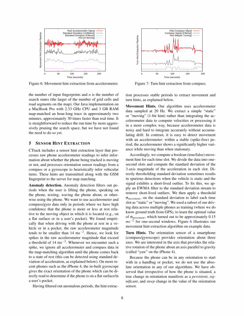
Figure 6: Movement hint extraction from accelerometer.

the number of input fingerprints and n is the number ofsearch states (the larger of the number of grid cells androad segments on the map). Our Java implementation ona MacBook Pro with 2.33 GHz CPU and 3 GB RAMmap-matched an hour-long trace in approximately twominutes, approximately 30 times faster than real time. Itis straightforward to reduce the run time by more aggres-sively pruning the search space, but we have not foundthe need to do so yet.

5 SENSOR HINT EXTRACTION

CTrack includes a sensor hint extraction layer that pro-cesses raw phone accelerometer readings to infer infor-mation about whether the phone being tracked is movingor not, and processes orientation sensor readings from acompass or a gyroscope to heuristically infer vehicularturns. These hints are transmitted along with the GSMfingerprint to the server for map matching.

Anomaly detection. Anomaly detection filters out pe-riods when the user is lifting the phone, speaking onthe phone, texting, waving the phone about, or other-wise using the phone. We want to use accelerometer andcompass/gyro data only in periods where we have highconfidence that the phone is more or less at rest rela-tive to the moving object in which it is located (e.g., ona flat surface or in a user’s pocket). We found empiri-cally that when driving with the phone at rest in a ve-hicle or in a pocket, the raw accelerometer magnitudetends to be smaller than 14 ms−2. Hence, we look forspikes in the raw accelerometer magnitude that exceeda threshold of 14 ms−2. Whenever we encounter such aspike, we ignore all accelerometer and compass data inthe map-matching algorithm until the phone comes backto a state of rest (this can be detected using standard de-viation of acceleration, as explained below). On more re-cent phones such as the iPhone 4, the in-built gyroscopegives the exact orientation of the phone which can be di-rectly read to determine if the phone is on a flat surface/ina user’s pocket.

Having filtered out anomalous periods, the hint extrac-

0 50 100 150 200

Tur

n H

int E

xtra

ctio

n P

ipel

ine

Time (seconds)

Raw Compass SignalCompass Signal (Filtered)

Hint (Maybe Turning)

Figure 7: Turn hint extraction from compass.

tion processes stable periods to extract movement andturn hints, as explained below.

Movement Hints. Our algorithm uses accelerometerdata sampled at 20 Hz. We extract a simple “static”or ”moving” (1-bit hint) rather than integrating the ac-celerometer data to compute velocities or processing itin a more complex way, because accelerometer data isnoisy and hard to integrate accurately without accumu-lating drift. In contrast, it is easy to detect movementwith an accelerometer: within a stable (spike-free) pe-riod, the accelerometer shows a significantly higher vari-ance while moving than when stationary.

Accordingly, we compute a boolean (true/false) move-ment hint for each time slot. We divide the data into one-second slots and compute the standard deviation of the3-axis magnitude of the acceleration in each slot. Di-rectly thresholding standard deviation sometimes resultsin spurious detections when the vehicle is static and thesignal exhibits a short-lived outlier. To fix this, we ap-ply an EWMA filter to the standard deviation stream toremove short-lived outliers. We then apply a thresholdσmovement , on the standard deviation to label each timeslot as “static” or ”moving”. We used a subset of our driv-ing data across multiple phones as training (where we doknow ground truth from GPS), to learn the optimal valueof σmovement , which turned out to be approximately 0.15ms−2 for one-second windows. Figure 6 illustrates ourmovement hint extraction algorithm on example data.

Turn Hints. The orientation sensor of a smartphone(compass/gyroscope) provides orientation about threeaxes. We are interested in the axis that provides the rela-tive rotation of the phone about an axis parallel to gravity(called “yaw” on the iPhone 4).

Because the phone can be in any orientation to startwith in a handbag or pocket, we do not use the abso-lute orientation in any of our algorithms. We have ob-served that irrespective of how the phone is situated, atrue change in orientation manifests as a persistent, sig-nificant, and steep change in the value of the orientationsensor.

8

Figure 8: Coverage map of our driving data set.

With compass data, the main challenge is that theorientation reported is noisy because metallic objectsnearby, or because the compass becomes uncalibrated.We solved this problem by applying a median filter witha three-second window on the raw orientation values,which filtered out non-persistent noise with consider-able success (a mean filter would also remove noise, butwould blur sharp transitions that we do want to observe).We then find transitions with a magnitude exceeding atleast 20 degrees and slope exceeding a threshold, whichwe fixed at 1.5 by experimentation.

Figure 7 illustrates a plot of the compass data with theturn marked, and the processing steps required to gener-ate a turn hint. We note that even after filtering, a truechange in orientation can sometimes be produced by thephone sliding around within a pocket or a bag, or turningfor reasons other than the car actually turning.

6 EVALUATION

In this section, we show that the trajectory matches pro-duced by CTrack are: (1) accurate enough to be use-ful for various tracking and positioning applications, (2)superior to sub-sampled GPS in terms of the accuracy-energy tradeoff, and (3) significantly better than strate-gies that reduce cellular fingerprints to point locationsbefore matching. We investigate how much each of thefour techniques used in CTrack —sequencing, window-ing, smoothing, and sensor hints—contribute to the gainsin accuracy.

6.1 Method and MetricsWe evaluate CTrack on 126 hours of real driving data inthe Cambridge-Boston area, collected from 15 AndroidG1 phones and one Nexus One phone over a period of4 months. We configured our phone library for the An-droid OS to continuously log the ground truth GPS loca-tion and the cell tower fingerprint every second, and theaccelerometer and compass at 20 Hz. Our data set covers3,747 road segments, amounts to 1,718 km of driving,and 560 km of distinct road segments driven. The dataset includes sightings of 857 distinct cell towers. Fig-ure 8 shows a coverage map of the distinct road segmentsdriven in our data set.

From 312 drives in all, we selected a subset of 53drives verified manually to have high GPS accuracy astest drives, amounting to 109 distinct km. We pickeda limited subset as test drives to ensure each test drivewas contained entirely within a small bounding box withdense training coverage. This is because evaluating thealgorithm in areas of sparse coverage (which many ofthe other 259 drives venture into) could bias results inour favor by reducing the number of candidate paths tomap-match to. For each test drive, we perform leave-one-out evaluation of the map-matching algorithm: we trainour algorithm on all 311 drives excluding the test drive,and then map-match the test drive using CTrack. We dothis to ensure enough training data for each drive, and atthe same time to keep the evaluation fair.

We compare CTrack to two other strategies in terms ofenergy and accuracy:

1. GPS k gets one GPS sample every k min-utes (k = 2,4), interpolates, and map-matches it usingVTrack [32].

2. Placelab-VTrack computes the best static local-ization estimate for each time instant using Placelab’stechnique [8], and matches the static estimates usingVTrack [32]. The VTrack paper shows that its HMMdoes much better than just matching each point to thenearest segment.

We use three metrics in our evaluation of accuracy:precision, recall, and geographic error. Our precisionand recall are similar to conventional precision and re-call, but take the order of matched segments in the trajec-tory into account. We say that a subset of segments in atrajectory T1 that also appears in trajectory T2 are alignedif those segments appear in T1 in the same order in whichthey appear in T2. Given a ground truth sequence of seg-ments G and an output sequence X to evaluate (producedby one of the algorithms), we run a dynamic program tofind the maximum length of aligned segments between Gand X . We define:

Precision =Total length o f aligned segments

Total length o f X(2)

Recall =Total length o f aligned segments

Total length o f G(3)

We estimated the ground truth sequencing of segmentsby map-matching GPS data sampled every second withVTrack [32], and manually fixing a few minor flaws inthe results.Geographic Error. Precision and recall are relevant toapplications that care about obtaining information at asegment-level, such as traffic monitoring. However, ap-plications such as visualization do not need to know theexact road segments traversed, but may want to identifythe broad contours of the route followed (e.g., mistakinga road for a nearby parallel road may be acceptable).

9

0

0.2

0.4

0.6

0.8

1

0 0.2 0.4 0.6 0.8 1

Pro

babi

lity

Precision (Matched Length/Output Length)

CTrackGPS 2 minGPS 4 minPlacelab+VTrack

Figure 9: CDF of Precision: Comparison.

To quantify this notion, we compute a third metric, ge-ographic error, which captures the spatial distance be-tween the ground truth and the matched output. We com-pute the maximum alignment between the ground truthtrajectory G and output trajectory X using dynamic pro-gramming. This alignment matches each segment S of Xto either the same segment S on G (if CTrack matchedthat segment correctly) or to a segment Swrong ∈ G (ifmatched incorrectly). Define the segment geographic er-ror to be the distance between S and Swrong for incor-rect segments, and 0 for correctly matched segments. Themean segment geographic error over all segments in X isthe overall geographic error.

6.2 Key FindingsThe key findings of our evaluation are:

1. CTrack has 75% precision and 80% recall in boththe mean and median, and a median geographic error of44.7 meters. We discuss what these numbers mean in thecontext of real applications below.

2. CTrack has 2.5× better precision and 3.5× smallergeographic error than Placelab+VTrack.

3. CTrack is equivalent in precision to map-matchingGPS sub-sampled every 2 minutes while consuming over2.5× less energy. It also reduces error (1− precision) bya factor of over 2× compared to sub-sampling GPS ev-ery 4 minutes, consuming a similar amount of energy.CTrack is 6× better than continuous WiFi sampling interms of battery lifetime on the Android platform.

4. The first step of CTrack, grid sequencing, is criti-cal. Without sequencing, CTrack effectively reduces tocomputing a (lat, lon) estimate from the best finger-print match, ignoring all other data. The median preci-sion without sequencing is only 50%. See Section 6.4for more detail.

5. We can extract movement and turn hints from rawsensor data with approximately 75% precision and re-call. These hints improve accuracy by removing spuriousloops and turns in the output. Using hints improves pre-cision by 6% and recall by 3%. See Section 6.5 for moredetail.

0

0.2

0.4

0.6

0.8

1

0 0.2 0.4 0.6 0.8 1

Pro

babi

lity

Recall (Matched Length/True Length)

CTrackGPS 2 minGPS 4 minPlacelab+VTrack

Figure 10: CDF of Recall: Comparison.

6.3 Accuracy ResultsFigure 9 shows a CDF of the map-matching precisionfor CTrack, GPS k (for k = 2,4 minutes) and Place-lab+VTrack. CTrack has a median precision of 75%,much higher than the both the energy-equivalent strat-egy of sub-sampling GPS every 4 minutes (48%), andPlacelab+VTrack (42%). In effect, CTrack has over 2×lower error (1− precision) than sub-sampling GPS ev-ery 4 minutes, and over 2.5× lower error than map-matching cellular localization estimates output by thePlacelab method. Also, CTrack has equivalent precisionto map-matching GPS sub-sampled every two minutes,while reducing energy consumption by approximately2.5× compared to this approach (Figure 2).

Figure 10 shows a CDF of the recall. All the strate-gies except GPS 4 min are equivalent in terms of re-call. Sub-sampling GPS every four minutes has poor re-call (median only 41%) because a four-minute samplinginterval misses significant turns in our input drives andfinds the wrong path. The fact that Placelab+VTrack hasidentical recall shows that simple static cellular localiza-tion does manage to recover a significant part of the in-put drive. However, converting cellular fingerprints di-rectly to points results in significant noise and long-livedoutliers, and hence produces a large number of incorrectsegments when map-matched directly (i.e., has low pre-cision).

To understand what 75% precision might mean interms of a an actual application, we refer readers toour work on VTrack [32], which studies the relation-ship between map-matching accuracy and the accuracyof two end-to-end applications: traffic delay monitor-ing and traffic hot-spot detection. We found that a me-dian precision of 85% was still useful for accurate traf-fic delay estimation. Our results for cellular (75%) areonly somewhat worse, and while not directly compara-ble, they suggest a significant portion of delay data fromCTrack would be useful.

For applications such as route visualization, or thosethat aggregate statistics over paths (e.g., to compute his-tograms over which of n possible routes is taken), or

10

0

0.2

0.4

0.6

0.8

1

0 0.2 0.4 0.6 0.8 1

Pro

babi

lity

Precision (Matched Length/Output Length)

With SequencingWithout Sequencing

Figure 11: Precision with and without grid sequencing.

those that simply show a user’s location on a map, gettingmost segments right with a low overall error is likely suf-ficient. Our median geographic error is quite low—just45 meters—suggesting CTrack would have sufficient ac-curacy for such applications. In contrast, the median ge-ographic error of the Placelab+VTrack approach is 156meters, over 3.5× worse than CTrack.Filtering using a confidence predictor. We investigatedwhether a confidence metric could be used to filter outdrives on which CTrack does poorly, thereby trading-off some recall for substantially better precision, whichwould be useful for accuracy-sensitive applications. Wefound two predictors, both weakly correlated with map-matching accuracy: (a) the 90th percentile distance ofsmoothed grids from the segments they are matched to,and (b) the mean difference (over all points P) in emis-sion score between the segment that P is matched toin the output, and the segment closest to P. The intu-ition is that a point far away from the road segment it ismatched to, or closer to a different road segment, implieslower confidence in the match. When applying these con-fidence filters to our output drives, we currently improvethe median precision from 75% to 86%, but lose sub-stantially in terms of recall, whose median reduces from80% to 35%). In future work, we plan to explore whetherboosting [12] can combine these weak confidence pre-dictors into a stronger one.

6.4 Benefit of SequencingWe elaborate on one of our key technical contributions:the idea that the first pass of grid sequencing before con-verting fingerprints to geographic locations is crucial toachieving good matching accuracy. We provide experi-mental evidence supporting this idea. We also show thatwindowing and smoothing help improve matching accu-racy, though to a lower degree.Impact of Sequencing. Figure 11 is a CDF that com-pares the precision of CTrack with and without the firstpass of grid sequencing. This figure shows that sequenc-ing is critical to achieving reasonable accuracy: with-out sequencing, the median precision drops from 75%

0.2

0.3

0.4

0.5

0.6

0.7

0.8

0.9

1

0 100 200 300 400 500

Pro

babi

lity

Ove

r 10

00 F

inge

rprin

ts

Geographic Spread Of Top 4 Exact Matches (meters)

Figure 12: Geographic spread of exact matches. Thedashed line shows the 80th percentile.

to 50%. The reason is that running CTrack without se-quencing amounts to reducing each fingerprint to its bestmatch in the training database, ignoring the sequence ofpoints.

As mentioned earlier, reducing a fingerprint to a singlegeographic location loses information because a givencellular fingerprint is seen from multiple locations quitefar apart. Figure 12 illustrates the CDF of this geographicspread. We selected 1000 fingerprints at random from ourtraining data. For each fingerprint F , we found all theexact matches for F , i.e. fingerprints F ′ with the exactsame set of towers in the training data as F . We orderedthe matches by similarity in signal strength, most similarfirst, and computed the geographic diameter of the top kmatches for each fingerprint (using k = 4).

The figure shows that over 20% of matching sets havea diameter exceeding 150 meters, and at least 10% havea diameter exceeding 400 meters. Recall that the meth-ods in Placelab (and RADAR, if applied to cellular data)would simply compute the centroid of the top k matches.This approach does not work well for sets with a largegeographic spread, and motivates the need for the funda-mentally different approach used in CTrack in which wekeep track of all possible likely locations, and then use acontinuity constraint to sequence these locations in twosteps.

Windowing and Smoothing. Table 1 shows the preci-sion and recall of CTrack with and without windowingand smoothing, two other heuristics used in CTrack. Wesee that each of these features improves the precision byapproximately 10%, which is a noticeable quantity. Therecall does not improve because the algorithm withoutwindowing/smoothing is good enough to identify mostof the segments driven: the heuristics mainly help elimi-nate loops in the output.

6.5 Do Sensor Hints Help?Figure 13 illustrates by example how turn hints extractedfrom the phone compass help in trajectory matching.Without using turn hints (Figure 13(a)), our algorithm

11

With WithoutPrec. Recall Prec. Recall

Windowing 75.4% 80.3% 65.6% 82.3%Smoothing 75.4% 80.3% 66.5% 82.5%

Table 1: Windowing and smoothing improve median tra-jectory matching precision.

finds the overall path quite accurately but includes sev-eral spurious turns and kinks, owing to errors in cellularlocalization. After including turn hints in the HMM, thefalse turns and kinks disappear (Figure 13(b)).

(a) Without turn hints (b) With turn hints

(c) Without movement hints (d) With movement hints

Figure 13: Sensor hints from the compass and accelerom-eter aid map-matching. Red points show ground truth andthe black line is the matched trajectory.

In Figure 13(c), the driver stopped at a gas station torefuel, which can be seen from the cluster of ground-truthGPS points. Before using movement hints, errors fromcellular localization were spread out, causing the map-matching to introduce a loop not present in the groundtruth (Figure 13(c)). After incorporating movement hints,the speed constraint in our HMM eliminates this loop be-cause it detects that the car would not have had sufficienttime to complete the loop (Figure 13(d)). We note a lim-itation of the movement hint: this kind of stop detectionworks because the phone was placed on the dashboard:if it had been in the driver’s pocket during refueling, themovement hints would not have helped had the drivergotten out of the car and been moving about.

Figure 14 is a CDF that compares the precision ofCTrack with and without sensor hints (both movementand turn). This figure shows that sensor hints improvethe median precision of matching by approximately 6%.While this may not seem huge, there exist several trajec-

0

0.2

0.4

0.6

0.8

1

0 0.2 0.4 0.6 0.8 1

Pro

babi

lity

Precision (Matched Length/Output Length)

With Sensor HintsWithout Sensor Hints

Figure 14: Precision with and without sensor hints.

0

0.1

0.2

0.3

0.4

0.5

0.6

0.7

0.8

0.9

1

0 0.2 0.4 0.6 0.8 1P

roba

bilit

yPrecision/Recall (0-1)

Move Hint PrecisionMove Hint Recall

Turn Hint PrecisionTurn Hint Recall

Figure 15: Precision/Recall CDF For Hint Extraction.

tories for which the hints do help significantly, suggest-ing that using them is a good idea when available. In ourexperience, the main benefit of the hints is in eliminat-ing the several “kinks” and spurious turns in the matchedtrajectory, which our metrics don’t adequately capture.

We used the ground truth GPS to measure how accu-rately our CTrack is able to extract individual movementand turn hints. We found that the median precision andrecall of both motion and turn hint extraction exceeds75%.

6.6 How Much Training?To quantify the amount of training data essentialto achieving good trajectory mapping accuracy withCTrack, we picked a pool of test drives at random,amounting to 5% of our data set (8 hours of data), anddesignated the remaining 95% as the training pool. Wepicked subsets of the training pool of increasing size, i.e.first using fewer drives for training, then using more. Ineach run, the training subset was used to train CTrackand then evaluated on the test pool. Figure 16 shows themean precision and recall of CTrack on the test pool asa function of the number of drive hours of training dataused to train the system. The accuracy is poor for verysmall training pools, as expected, but encouragingly, itquickly increases as more training data is available. Thealgorithm performs almost as accurately with 40 hoursof training data as with 120, suggesting that 40 hours oftraining is sufficient for our data set.

12

0.5

0.55

0.6

0.65

0.7

0.75

0.8

0 20 40 60 80 100 120

Pre

cisi

on/R

ecal

l (0-

1)

Drive Hours Of Training Data (Randomly Selected)

PrecisionRecall

Figure 16: Prec./Recall vs Training Data Size.

0

0.2

0.4

0.6

0.8

1

0 2 4 6 8 10 12

Fra

ctio

n O

f Tes

t Roa

d S

egm

ents

Count of Times Traversed In Training Pool

Figure 17: CDF of Drive Counts, 40 Hrs Training Data.

The 40-hour number, of course, is specific to the ge-ographic area we covered in and around Boston, and tothe test pool. To gain more general insight, we measurethe drive count for each road segment in the test pool, de-fined as the number of times the segment is traversed byany drive in the training pool. Figure 17 shows the dis-tribution of test segment drive counts corresponding to40 hours of training data. While the mean drive count isapproximately 3, this does not mean each road segmenton the map needs to be driven thrice to achieve good ac-curacy. As the graph shows, about 60% of the test seg-ments were not traversed even once in the training pool,but we can still map-match many of these segments cor-rectly. The reason is that they lie in the same grid cellas some nearby segment that was driven in the trainingpool. This result promising because it suggests that train-ing does not have to cover every road segment on the mapto achieve acceptable accuracy.

7 RELATED WORK

Placelab performed a comprehensive study of GSM lo-calization and used a fingerprinting scheme for cellularlocalization [8]. RADAR used a similar fingerprintingheuristic for indoor WiFi localizations [3], and our map-matching emission score is inspired by these methods.However, neither Placelab nor RADAR address the prob-lem of trajectory matching, and are concerned with theaccuracy of individual localization estimates, rather than

finding the optimal sequencing of estimates. As shownby our results, this sequencing step is critical: applying amap-matching algorithm directly to Placelab-style loca-tion estimates results in significantly worse accuracy (bya factor of over 2×) compared to CTrack.

Letchner et al. [17] and our previous work onVTrack [32] use HMMs for map-matching. However,these previous algorithms use and process (lat, lon) co-ordinates as input and use a Gaussian noise model foremissions, and are hence unsuitable and inaccurate formap-matching cellular fingerprints, as shown by our re-sults. Nor do they use sensor hints.

CompAcc [10] proposes to use smartphone compassesand accelerometers to find the best match for a walkingtrail by computing directional “path signatures” for thesetrails. They do not use cell towers. However, from ourunderstanding, the paper uses absolute values of compassreadings. This approach did not work in our experiments,because the absolute orientation of a phone can be quitedifferent depending on whether it is in a driver’s pocket,on a flat surface, or held in a person’s hand. For this rea-son, we chose to use boolean turn hints instead, whichare more robust and can be accurately computed regard-less of changes in the phone’s initial orientation or posi-tion. For extracting motion hints and detecting walkingand driving using the accelerometer, we use algorithmssimilar to those in [27, 31, 26].

Some previous papers [9, 23, 16] have proposedenergy-efficient localization schemes that reduce re-liance on continuously sampling GPS by using a moreenergy-efficient sensor, such as the accelerometer, totrigger sampling GPS. RAPS [23] also uses cell towers to“blacklist” areas where GPS accuracy is low and henceGPS should be switched off, to save energy. However,none of these papers address trajectory matching or pro-pose a GPS-free, accurate solution for map-matching.

Skyhook [29] and Navizon [20] are two commercialproviders for WiFi and Cellular localization, providingdatabases and APIs that allow programmers to submitWiFi access point(s) or cell tower(s) and look up thenearest location. However, to the best of our knowl-edge, they do not use any form of sequencing or map-matching, and focus on providing the best static local-ization estimate.

8 CONCLUSION

We described CTrack, an energy-efficient, GPS-free sys-tem for trajectory mapping using cellular tower finger-prints. The key lesson we learned was that sequencingcellular fingerprints before matching them is critical toachieving good accuracy. On smartphones, our CTrackimplementation uses close to zero extra energy whileachieving good mapping accuracy, making it a good wayto distribute collaborative trajectory-based applications

13

like traffic monitoring to a huge number of users withoutany associated energy consumption or battery drain con-cerns. A GPS-free approach to trajectory matching alsoopens up the possibility of providing more fine-grainedlocation services on the world’s most popular, cheapestphones that do not have GPS, but that do have GSM con-nectivity.

ACKNOWLEDGMENTS

This work was supported by the National Science Foun-dation under grant CNS-0931550.

REFERENCES[1] Analog Devices AD9864 Datasheet: GSM RF Front End and

Digitizing Subsystem. http://www.analog.com/static/imported-files/data sheets/AD9864.pdf.

[2] Analog Devices, Inc. ADXL330: Small, Low Power, 3-Axis +/-3g iMEMS Accelerometer (Data Sheet), 2007. http://www.analog.com/static/imported-files/data sheets/ADXL330.pdf.

[3] P. Bahl and V. Padmanabhan. RADAR: An In-building RF-basedUser Location and Tracking System. In INFOCOM, 2000.

[4] N. Balasubramanian, A. Balasubramanian, andA. Venkataramani. Energy Consumption in Mobile Phones: AMeasurement Study and Implications for Network Applications.In IMC, 2009.

[5] F. Ben Abdesslem, A. Phillips, and T. Henderson. Less is more:Energy-efficient Mobile Sensing with SenseLess. In MobiHeld,2009.

[6] GPS and Mobile Handsets. http://www.berginsight.com/ReportPDF/ProductSheet/bi-gps4-ps.pdf.

[7] A. Boustani, L. Girod, D. Offenhuber, R. Britter, M. I. Wolf,D. Lee, S. Miles, A. Biderman, and C. Ratti. Investigation of theWaste Removal Chain Through Pervasive Computing. IBMJournal of Research and Development, 2010.

[8] M. Y. Chen, T. Sohn, D. Chmelev, D. Haehnel, J. Hightower,J. Hughes, A. Lamarca, F. Potter, I. Smith, and A. Varshavsky.Practical Metropolitan-scale Positioning for GSM Phones. InUbiComp, 2006.

[9] I. Constandache, S. Gaonkar, M. Sayler, R. Choudhury, andL. Cox. EnLoc: Energy-Efficient Localization for MobilePhones. In INFOCOM, 2009.

[10] I. Constandache, R. Roy Choudhury, and I. Rhee. CompAcc:Using Mobile Phone Compasses and Accelerometers forLocalization. In INFOCOM, 2010.

[11] Fedex intros Senseaware Sensor for Tracking Packages.http://www.electronista.com/articles/09/11/27/senseaware.sensor.sends.temps.drops.more.

[12] Y. Freund and R. E. Schapire. A Decision TheoreticGeneralization of Online Learning and an Application toBoosting. In EuroCOLT, 1995.

[13] S. Gaonkar, J. Li, R. R. Choudhury, L. Cox, and A. Schmidt.Micro-Blog: Sharing and Querying Content through MobilePhones and Social Participation. In MobiSys, 2008.

[14] Information On Human Exposure To Radiofrequency FieldsFrom Cellular and PCS Radio Transmitters.http://www.fcc.gov/oet/rfsafety/cellpcs.html.

[15] iCartel. http://icartel.net/icartel-docs/.[16] M. B. Kjærgaard, J. Langdal, T. Godsk, and T. Toftkjær.

EnTracked: Energy-efficient Robust Position Tracking forMobile Devices. In MobiSys, 2009.

[17] J. Krumm, J. Letchner, and E. Horvitz. Map Matching withTravel Time Constraints. In SAE World Congress, 2007.

[18] K. Lin, A. Kansal, D. Lymberopoulos, and F. Zhao.Energy-accuracy Trade-off for Continuous Mobile DeviceLocation. In MobiSys, 2010.

[19] LoJack Car Security System For Stolen Vehicle Recovery.http://www.lojack.com.

[20] Navizon. http://www.navizon.com.[21] Qualcomm Transportation: OmniTRACKS Mobile

Communications System.http://www.qualcomm.com/products services/mobile content services/enterprise/omnitracs.html.

[22] OpenStreetMap. http://www.openstreetmap.org.[23] J. Paek, J. Kim, and R. Govindan. Energy-efficient Rate-adaptive

GPS-based Positioning for Smartphones. In MobiSys, 2010.[24] PNI Corporation. MicroMag3 3-Axis Magnetic Sensor Module.

http://www.sparkfun.com/datasheets/Sensors/MicroMag3%20Data%20Sheet.pdf.

[25] Qualcomm inGeo Service.http://www.qualcomm.com/innovation/stories/ingeo.html.

[26] L. Ravindranath, C. Newport, H. Balakrishnan, and S. Madden.Improving Wireless Network Performance Using Sensor Hints.In NSDI, 2011.

[27] S. Reddy, M. Mun, J. Burke, D. Estrin, M. Hansen, andM. Srivastava. Using Mobile Phones to DetermineTransportation Modes. Transactions on Sensor Networks, 6(2),2010.

[28] RunKeeper. http://runkeeper.com.[29] Skyhook. http://www.skyhookwireless.com.[30] Telit GE865 Datasheet.

http://www.telit.com/module/infopool/download.php?id=1666.[31] A. Thiagarajan, J. Biagioni, T. Gerlich, and J. Eriksson.

Cooperative Transit Tracking Using GPS-enabled Smart-phones.In SenSys, 2010.

[32] A. Thiagarajan, L. Sivalingam, K. LaCurts, S. Toledo,J. Eriksson, S. Madden, and H. Balakrishnan. VTrack: Accurate,Energy-Aware Road Traffic Delay Estimation Using MobilePhones. In SenSys, 2009.

[33] TomTom. http://www.tomtom.com.[34] Trash Track. http://senseable.mit.edu/trashtrack.[35] A. J. Viterbi. Error Bounds for Convolutional Codes and an

Asymptotically Optimum Decoding Algorithm. In IEEETransactions on Information Theory, 1967.

[36] Y. Wang, J. Lin, M. Annavaram, Q. A. Jacobson, J. Hong,B. Krishnamachari, and N. Sadeh. A Framework of EnergyEfficient Mobile Sensing for Automatic User State Recognition.In MobiSys, 2009.

14