Accurate, Dense and Robust Multi-View Stereopsis

Yasutaka Furukawa and Jean PoncePresented by Rahul Garg and Ryan Kaminsky

Agenda

• Problem Statement

• Multi-view Stereo Taxonomy

• Algorithm

• Results

• Comparison to other works

• Questions

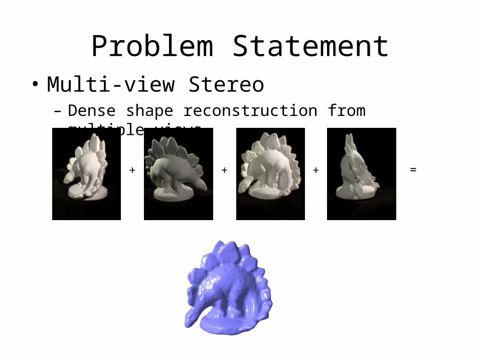
Problem Statement• Multi-view Stereo

– Dense shape reconstruction from multiple views

+ + + =

Multi-View Stereo Taxonomy

• Scene Representation

• Photoconsistency Measure

• Visibility Model

• Shape Prior

• Reconstruction algorithm

• Initialization

S. M. Seitz, B. Curless, J. Diebel, D. Scharstein, and R. Szeliski

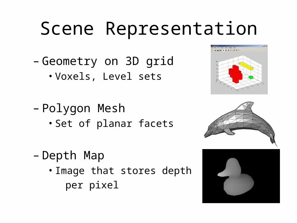
Scene Representation

– Geometry on 3D grid• Voxels, Level sets

– Polygon Mesh• Set of planar facets

– Depth Map• Image that stores depth

per pixel

Photoconsistency Measure

• Definition: Measures visual compatibility of reconstruction with input images

– Scene Space• Project part of reconstruction into images, measure

closeness• Measures: Variance , sum of squared distances, normalized

cross-correlation

– Image Space• Use scene geometry to transform image to different view,

measure error of predicted vs. actual (prediction error)

Visibility Model

• Definition: Views to consider when evaluating photo consistency– Geometric

• Explicitly model geometry of the scene

– Quasi-Geometric• Approximate geometric reasoning

– Outlier based approaches• Treat occlusions as outliers

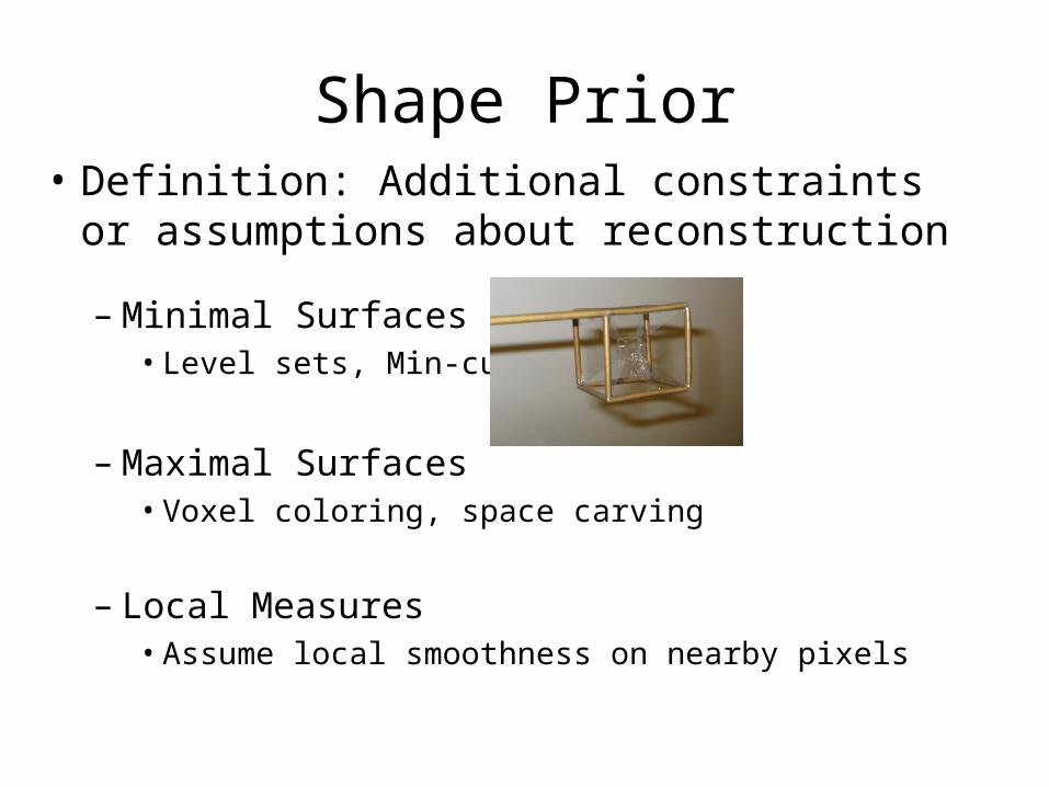
Shape Prior• Definition: Additional constraints or

assumptions about reconstruction

– Minimal Surfaces• Level sets, Min-cut

– Maximal Surfaces• Voxel coloring, space carving

– Local Measures• Assume local smoothness on nearby pixels

Reconstruction Algorithm

• Optimize cost function– Voxels, graph cut, level sets, meshes

• A set of consistent depth maps

• Feature extraction, matching, surface fitting

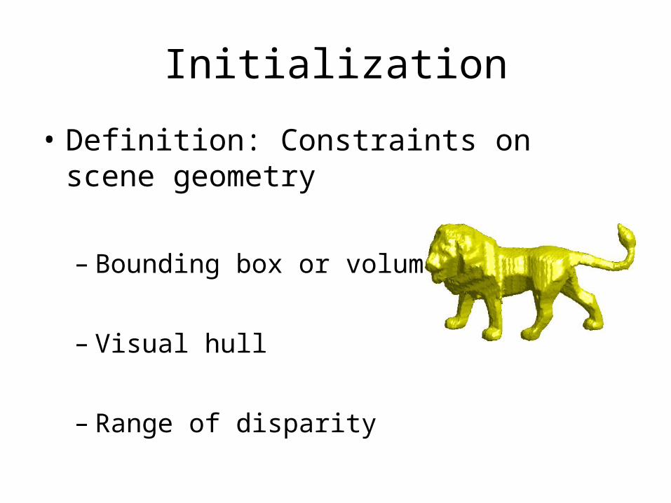
Initialization

• Definition: Constraints on scene geometry

– Bounding box or volume

– Visual hull

– Range of disparity

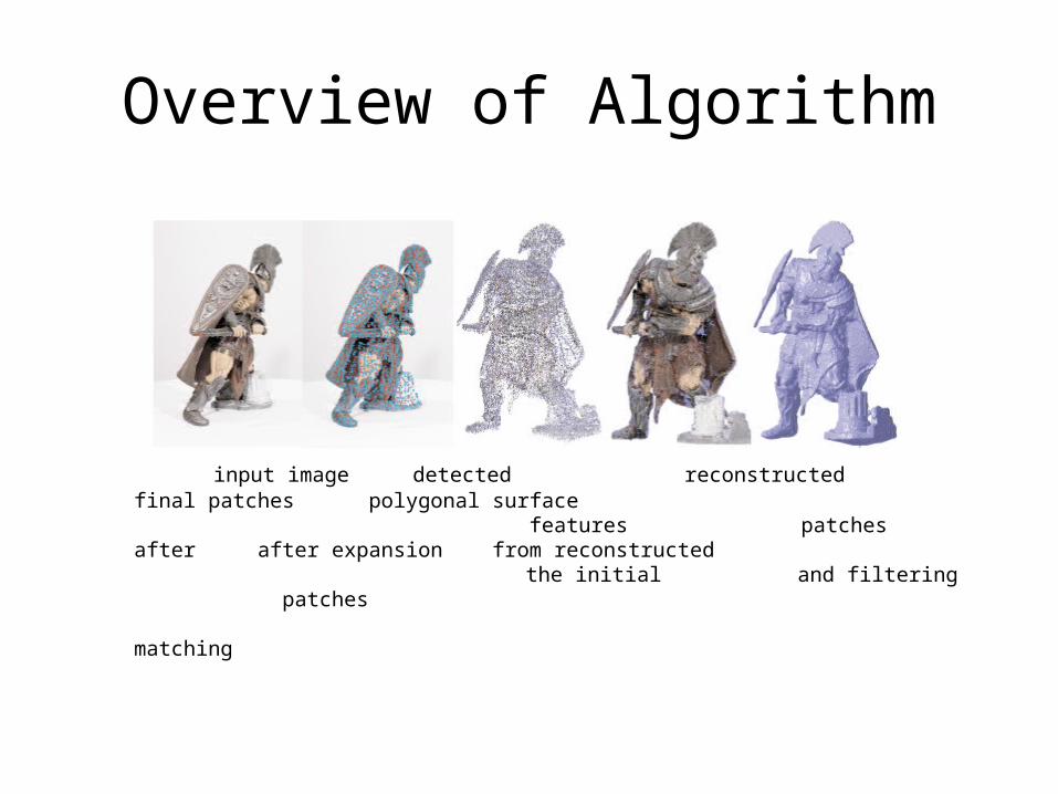
Overview of Algorithm

input image detected reconstructed final patches polygonal surface features patches after after expansion from reconstructed the initial and filtering patches matching

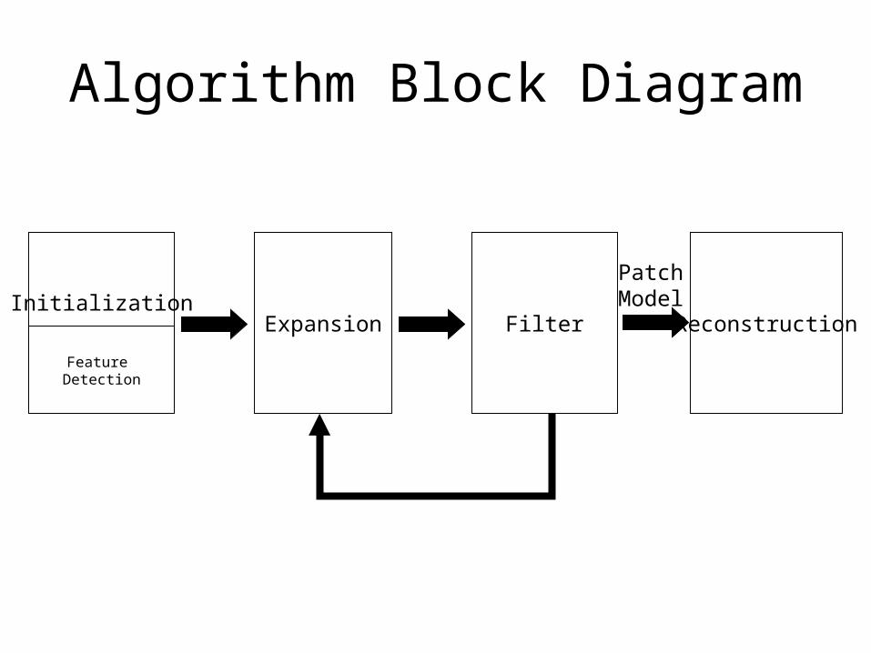
Algorithm Block Diagram

InitializationExpansion Filter

Feature Detection

Reconstruction

Patch Model

Init

• Detect features using Harris Corner and DoG

• Feature matching to generate sparse set of patches

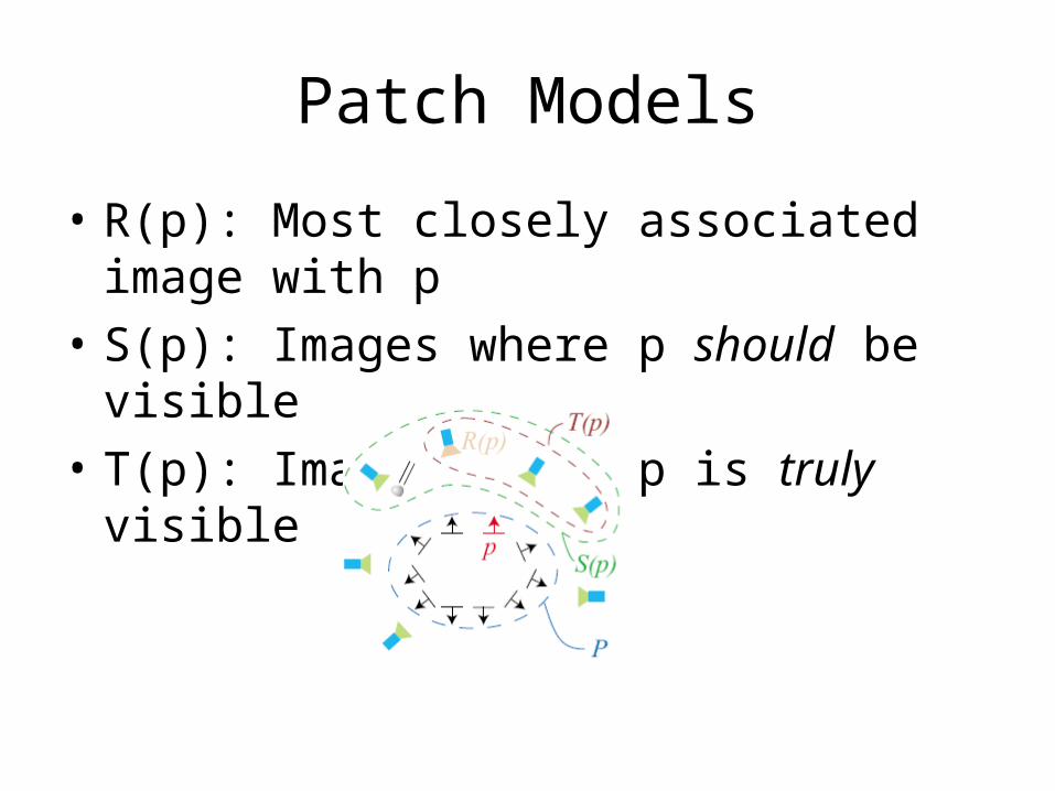
Patch Models

• R(p): Most closely associated image with p

• S(p): Images where p should be visible

• T(p): Images where p is truly visible

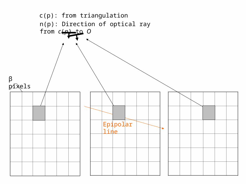
β pixels

Epipolar line

c(p): from triangulation

n(p): Direction of optical ray from c(p) to O

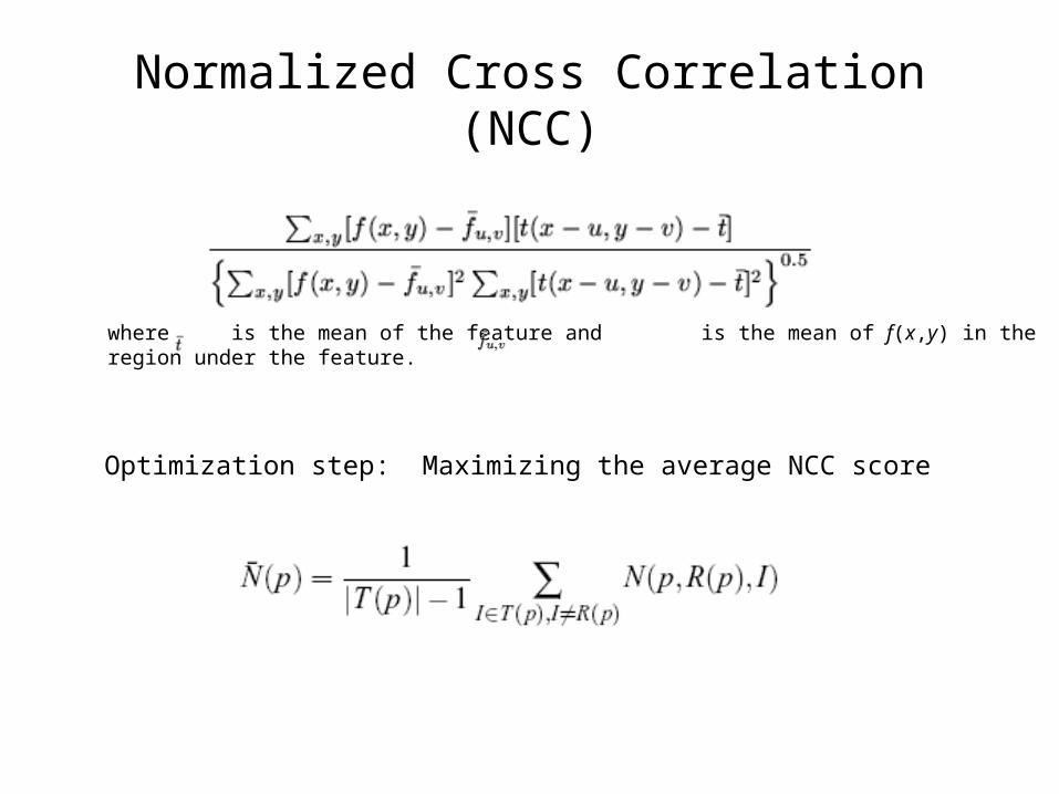
Normalized Cross Correlation (NCC)

Optimization step: Maximizing the average NCC score

where   is the mean of the feature and      is the mean of f(x,y) in the region under the feature.

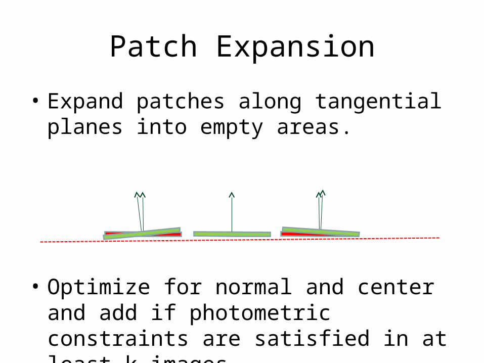
Patch Expansion

• Expand patches along tangential planes into empty areas.

• Optimize for normal and center and add if photometric constraints are satisfied in at least k images.

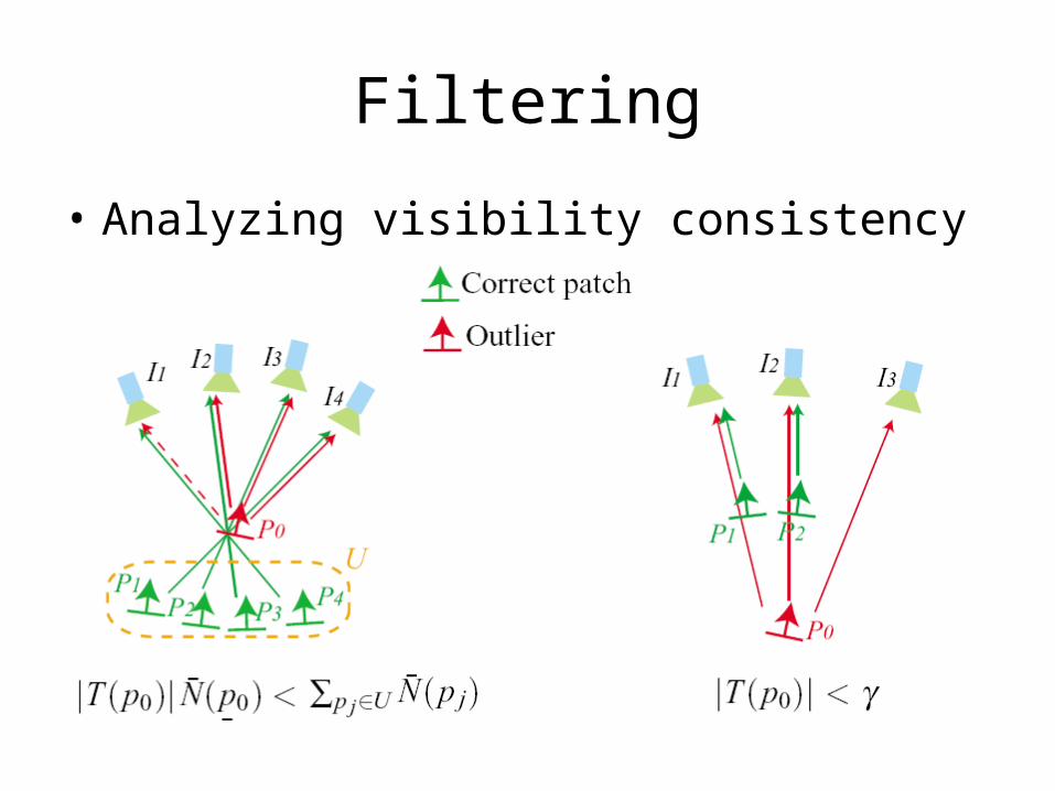
Filtering

• Analyzing visibility consistency

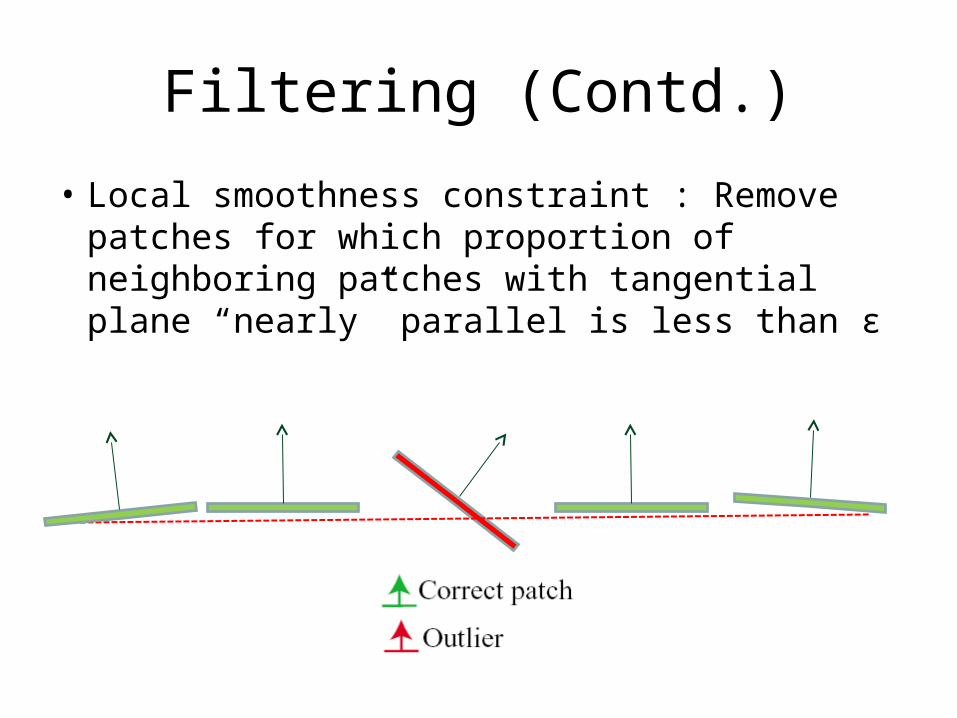
Filtering (Contd.)

• Local smoothness constraint : Remove patches for which proportion of neighboring patches with tangential plane “nearly” parallel is less than ε

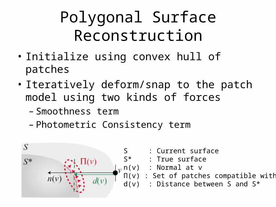
Polygonal Surface Reconstruction

• Initialize using convex hull of patches

• Iteratively deform/snap to the patch model using two kinds of forces– Smoothness term– Photometric Consistency term

S : Current surfaceS* : True surfacen(v) : Normal at vΠ(v) : Set of patches compatible with vd(v) : Distance between S and S*

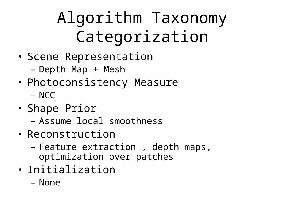
Algorithm Taxonomy Categorization

• Scene Representation– Depth Map + Mesh

• Photoconsistency Measure– NCC

• Shape Prior– Assume local smoothness

• Reconstruction– Feature extraction , depth maps, optimization over

patches

• Initialization– None

Results

Patch Model Polygonal Surface Model

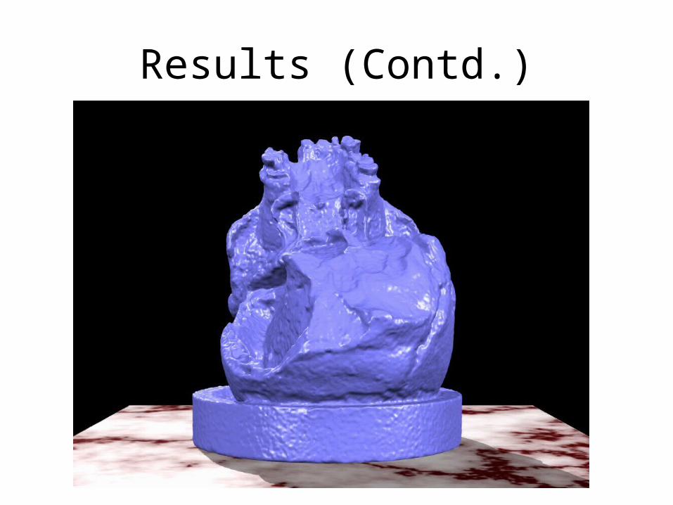
Results (Contd.)

Results (Contd.)

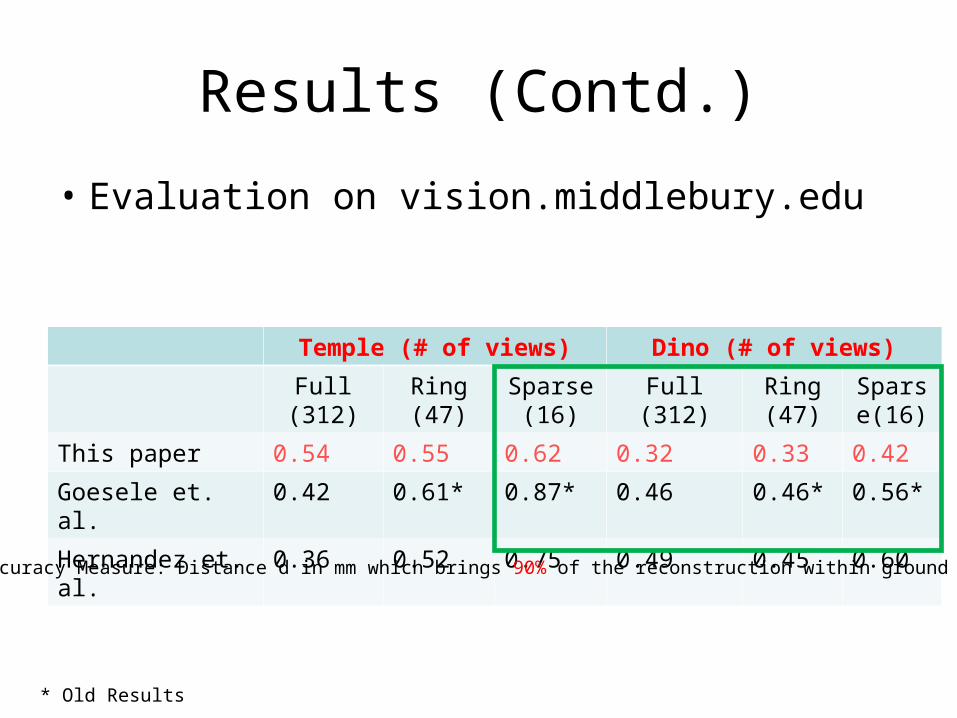
• Evaluation on vision.middlebury.edu

Temple (# of views) Dino (# of views)

Full(312)

Ring(47)

Sparse(16)

Full(312)

Ring(47)

Sparse(16)

This paper 0.54 0.55 0.62 0.32 0.33 0.42

Goesele et. al. 0.42 0.61* 0.87* 0.46 0.46* 0.56*

Hernandez et. al. 0.36 0.52 0.75 0.49 0.45 0.60

Accuracy Measure: Distance d in mm which brings 90% of the reconstruction within ground truth

* Old Results

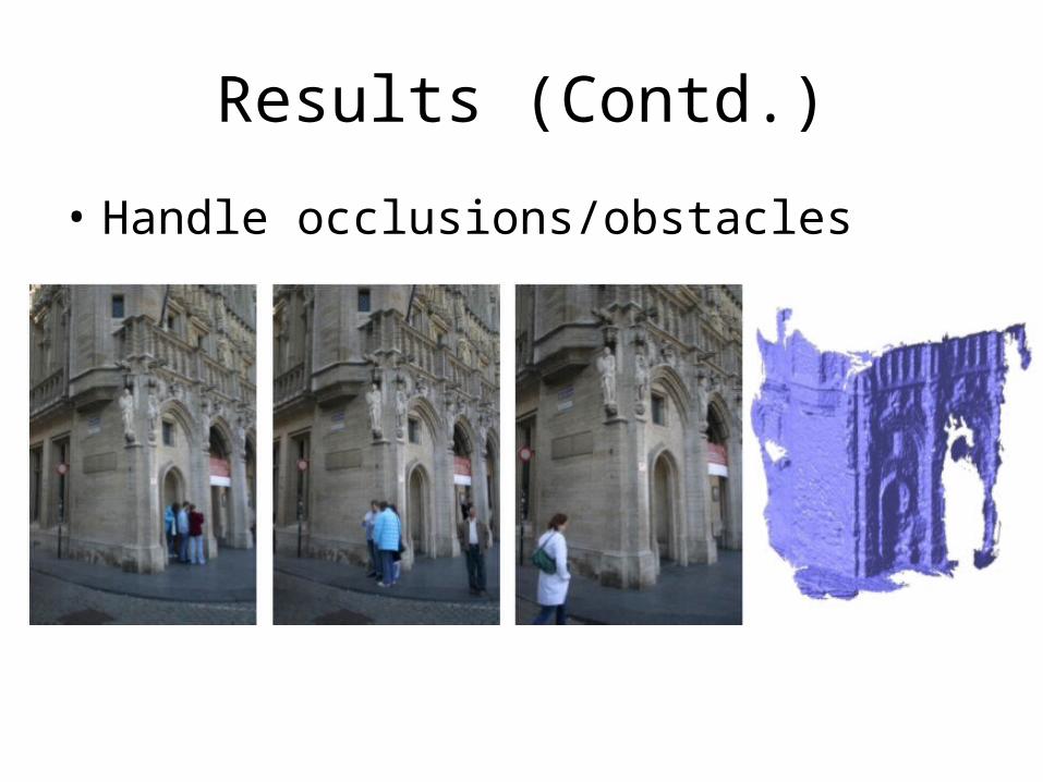
Results (Contd.)

• Handle occlusions/obstacles

Similar Approaches

• Setup similar to Goesele et al. (ICCV’07) – initialize patches, expand and optimize for position and normal

This Paper Goesele et. al.

Initialize patches using triangulated points

Initialize using Structure from Motion features

Explicit occlusion handling Occlusion handling through outlier removal and view selection, prioritize patch candidates for expansion

Questions

• Pose the problem as an optimization problem simultaneously accounting for local smoothness, photo consistency, occlusion

• Convergence of Expand/Filter – do more iterations lead to better reconstructions?

• Occlusion/Outlier handling – results on more datasets

• Advantages of patch model – Adaptive Resolution, generalizes to large number of object classes