Accuracy Analysis of Estimation of 2–D FlowProfile in Conduits by Results of Multipath

Flow Measurements

Mikhail Ronkin and Aleksey Kalmykov

Ural Federal University, pr. Mira, 19, Yekaterinburg, 620002,Russian Federation

z sm@mail.ru

Abstract. The paper presents a model of distorted velocity distributionof a flow in conduit, which passes through its bent section. The proposedmodel is properly analyzed. An algorithm for recovering the pipe profileby multipath ultrasonic measurements in the presence of a priori infor-mation is proposed. Numerical simulations with the proposed algorithmare performed as well.

Keywords: flow measurements, flow profile, multipath flowmeter

1 Introduction

In practice, it is important to know the set of values of the stream head of a flowin each section of the pipeline. The flow head is one of the main characteristicsof the conduit. When the flow passes through a bent section (such as elbow orvalve, etc.), its head gets lost. In practice, losses of the head are determined byexperiments [1]. The loss of head is connected with the flow profile distortion.There is a symmetric flow profile in a long straight section of pipeline (Fig. 1a,b).However, when flow passes a bent section (such as elbow, valve, etc.), the flowprofile, i.e., the distribution of velocity in the cross section of the pipe, becomesdistorted (Fig. 1 c,d). Thus, the profile of flow characterizes a bent section ofthe pipe [1].

One way to determine the flow profile is to recover it by ultrasonic multi-path flow measurements. The ultrasonic technology allows measurement of thevelocity distribution in a number of planes between two transducers/receivers ofacoustic waves as it is shown in Fig. 2a. The distortion of a flow profile can berecovered by approximation of such measured values in a sufficient number ofplanes [2].

The task of ultrasonic measurement of the flow rate is the radar task ofmeasurement of propagation time in an investigated media. The emitted waveaccelerates when moving in the direction of a flow and slows down in the oppositedirection (Fig. 2b). The velocity of a flow is calculated as a difference of measuredtimes of propagation:

t12 =L

c+ vl cosα, t21 =

L

c− vl cosα, (1)

143

vl =∆tc2

2L cosα, vz =

∆tc2

2Ltanα, (2)

where t12 is the time of propagation in the flow direction; t21 is the time ofpropagation in the opposite direction; c is the speed of acoustic wave; α is theangle between direction of the flow and direction of the wave propagation; L isthe length of the wave path in the investigated media; vl is the projection of theflow velocity on the wave path; vz is the velocity in z–direction of the flow [3].

The velocity profile is always distributed not uniformly through the cross–section area of a pipe. This means that velocity in the central region is usuallyhigher than near the wall. The measured value of velocity vl is the average ofthis distribution in the direction of the path. Measured value usually differs fromaverage velocity through the whole cross section vc:

vl =

∫ L

0

v(l)dl, Q =

∫

s

v(x, y)dS, (3)

k =Q

πR2vl, (4)

where v(l) is the distribution of velocity in the direction of the wave propagation;Q is the flow rate; v(x, y) is the distribution of velocity through the whole cross–section of the conduit; R is the radius of the pipe; S is the cross–section area ofthe pipe; k is the meter factor, which is connected with the measured and actualflow rate [3].

Equation (4) is valid for any symmetric flow. However, in the case of asym-metric propagation of the flow wave patch, the flow rate would be calculatedwith error. The type of function v(x, y) for asymmetric flow does not have gen-eral analytical expression. The function of flow distribution strongly depends onthe conduit configuration, and its characteristics (such as material, roughness,temperature of the controlled media, etc.). The error of the calculated flow ratefor a single path flow meter can achieve a 10% and be even larger [3].

The meter factor can be calibrated in laboratory conditions. Such calibrationis generally performed on a long straight section of a conduit where a symmetryflow profile takes place [3]. In the case of multipath flow meter, all asymmetricfeatures are assumed to be present for calibration of a symmetric flow. In -practice, it is necessary to have more than 4 paths to consider the meter factor as1 with error less than 0.1% [4, 5]. However, the solution of the task of recoveringa flow profile with such accurate flow measurements is an open issue.

For some types of flow profiles, the analytical expression has been obtained bySalami [6]. Based on his works, some authors proposed analysis of configurationof the multipath measurements and suggested some interpretations of analyti-cal profiles [4–8]. The solution of the profile recovering problem by ultrasonicflow measurements was only proposed on the basis of ultrasonic tomographyor by Abel’s integration transform, which doesn’t take into account asymmetryfeatures of flow [2, 9].

144

In this work, a technique is suggested for recovering the flow profiles using themultipath measurements and a priori information about discretionary function,which can be determined for each type of a bent section of the conduit.

Fig. 1. Flow profiles for a) m=2, a=0; b) m=5, a=0; ) m=5, a=0.3; d) m=5, a=0.7

2 Model of flow profile

The model of flow profile, which have been proposed by authors [6, 7] can beconsidered as a particular case of a flow profile that has passed through a conduitsection, whose specified characteristic determines the distortion of the velocitydistribution. The proposed model and generalized approach can be analyzedregarding to the accuracy of the profile recovering.

In general, the flow rate could be calculated as an integral of velocity distri-bution over the cross-section area as

Q =

∫

s(z)

vz(x, y)dS =

∫ x2=R

x1=−R

[∫ y2=√(R2−x2)

y1=−√(R2−x2)

vz(x, y)dy

]dx, (5)

Thus

Q =

∫ R

−Rvz(x)dx =

c2 tan(α)

2

∫ R

−R∆t(x)dx, (6)

where ∆t(x) is the distribution of difference values of measured propagation timein the flow direction and in the opposite one versus the coordinate. In theoryof numerical integration, it is proposed to substitute the integral by sum withspecified weight, which may be chosen, for instance, by criteria of optimal distri-bution of nodes locations and corresponding coefficients (the Gauss quadrature

145

Fig. 2. Schematic draw picture a) multipath flowmeter and b) the center plane cut, ηiis the ith plane

method). The solution is presented in Table 1.

ξ =x

R

∫ R

−R∆(x)dx → R

∫ 1

−1∆(ξ)dξ = R

n∑

i

λi∆t(ξ), (7)

where ξ is the normalized coordinate of the measurement plane, λi is the coef-ficient of weight function (determined by solution of the Gauss quadrature taskfor number of measurements); ∆t(ξi), i = 1, 2 . . . n are differences of propagationtimes in planes with coordinate ξi; n is the number of planes. In the case of a

Table 1. Solution of Gauss quadrature task [10]

n=2 n=3 n=4 n=5

λi ± 0,5773 0 ± 0,7746 ± 0.3400 ± 0.8611 0 ± 0.5385 ± 0.9062

ξi 1 0.8889 0.5556 0, 6521 0,3479 0.5689 0.2369 0.4786

multipath flow meter, the flow rate can be calculated in accordance with (6) as

Q = kc2R tan(α)

2

n∑

i

λi∆t(ξi) = kn∑

i=1

λivz(ξi), (8)

where the meter factor k can be considered as 1 if there are more than 4 measuredplanes [4]. There are many profiles proposed by Salami [6], which have beenverified by experiments. For instance, authors [2] noted that profile of flow thatpasses through a single elbow could be expressed as follows:

vz(r, ϕ)

v0= sin

(π2

(1− r)1/m)

+ α sin(π(1− r)1/2

)exp(−0.2ϕ) sin(ϕ), (9)

146

where vz(r, ϕ) is the velocity distribution in cylindrical coordinates; r is theradius; ϕ is the angle; v0 is the velocity of flow at the center of cross-section(vz(0, 0) = v0); α is the velocity of flow at the center of cross-section; m isthe coefficient of symmetric flow profile, which characterizes the flow profiledepending on velocity if asymmetric coefficient is equal to zero. In the originalwork [6], the author proposed values m = 5, α = 0.3. The first part of theright side of equation (4) corresponds to the symmetric part of the flow, and thesecond part corresponds to asymmetry distortion with coefficient α [6]. Withoutasymmetry distortion, the flow rate is calculated according to the equations(8)-(9) as

Q =

∫

S

sin(π

2(1− r) 1

m

)dS =

∫ 2π

0

∫ R

−Rsin(π

2(1− r) 1

m

)rdrdϕ, (10)

Q = kRn∑

i=1

λivz (ξi) . (11)

For symmetric model of flow (10, 11) calibration m = f(k) = f(Q/v0) couldbe performed. Normalized profiles are shown in Fig. 1 a,b. It can be notedthat profile with m=2 corresponds to the laminar flow mode, and cannot beconsidered in model. Profile with m=5 corresponds to the turbulent mode [2].It is well known that the profile of a flow changes toward symmetry distributionwith distance from a section of the conduit, which caused distortion [3]. So, itmay be supposed that the influence of the second part of equation (9) decreases asasymmetric coefficient tends to zero with increasing distance from the distortedsection of the conduit. Based on the condition of constant flow (Q(z) = const)it should be noted that m is also changing with distance from the section of theconduit that caused the distortion.

It may be proposed that type of the second part of the right side of equation(9) depends on the type of section of the conduit, which caused distortion. Suchexpressions can be defined theoretically or from experiments. In this work, typeof the profile (9), which corresponds to signal elbow [2], is considered. Profiles offlow for m = 5, α = 0.3 and α = 0.7 are shown in Fig. 2c,d. It has been mentionedabove that in each measurement plane, the value of velocity is the integral overthe direction of acoustic wave propagation. The normalized measured velocityin the plane with coordinate xi corresponds to equation (9) can be expressed as

vz(xi)

v0=

=

∫ +A

−A

[sin(π

2(1− (x2i + y2)1/2

)1/m]+

[α sin

(π(

1− (x2 + y2)1/2)1/2)]

×

× exp(−0.2 arctan

(y

xi

)sin

(arctan

(y

xi

))dy, (12)

147

where A =√R2 − x2i . Denote:

F1 (xi,m) =

∫ +A

−A

[sin(π

2(1− (x2i + y2)1/2

)1/m]dy, (13)

F2 (xi) =

[α sin

(π(

1− (x2 + y2)1/2)1/2)]

×

× exp(−0.2 arctan

(y

xi

)sin

(arctan

(y

xi

))dy. (14)

Consequently,vz (xi)

v0=F1 (xi,m) +αF2 (xi) , (15)

where F1(xi,m) is the function, which characterizes symmetric part of flow,F2(xi) is the function, which characterizes an asymmetric part of flow when itpasses through a bent section. Expression of the flow rate corresponding to (15)is

Q =

∫ R

−Rvz(x)dx = v0

∫ R

−R[F1(xi,m) + αF2(xi)] dx ≈ kR

n∑

i=1

λivz(ξi). (16)

In accordance with (15), the flow rate can be expressed as

Q ≈ v0Rn∑

i

λi [F1(ξi,m) + αF2(ξi)] . (17)

In equation (17), the meter factor is not used because since it is included in thecalibration dependence for F1(xi,m). From equation (17) in accordance with(11) and (16), the symmetric flow rate normalized on v0 can be expressed as

Qcv0

= R

[k

n∑

i=1

λivz (ξi)− αv0n∑

i=1

λiF2(ξi2)

]= f−1(m), (18)

where f−1(m) = Qc/v0 denotes the calibration relation in coordinates f(Qc/v0).Such calibration can be implemented because of symmetry of function F1(xi,m)and symmetry of profile Qc. Hence, if we know the flow rate under symmetricconditions and radius of the pipe, we can deduce v0.

There are three unknown parameters in equation (17): v0 is the value ofvelocity at the center of the pipe cross-section; m is the coefficient of symmet-ric part of flow; α is the asymmetric coefficient. Here, it is assumed that typeof function F2(xi) is known as a function of distorted section of the conduit.Relation m = f(F1(x,m)) = f(Q/vc) assumed to be known from preliminarycalibrations on a long straight pipeline. The determination of parameters namedabove requires solution of the system of equations for each parameter. The po-sition of planes (xi) is supposed to be chosen here in accordance with Table 1

148

and from symmetry of F1(xi,m). The solution of the system mentioned abovehas the following expression:

α = [(vz(x3)− vz(x1))F1(x1,m)]/[F2(x2)vz(x1)− vz(x3)F2(x1)],

v0 = [F2(x3)vz(x1)− vz(x3)F2(x1)]/[F1(x1,m) (F2(x1)− F2(x3))],

n∑i=1

λiF1(xi,m) =[k

n∑i=1

λivz(xi)− αv0n∑i=1

λiF2(xi)]/v0 = f−1(m).

(19)

Here, the first and the second equations are calculated depending on F1 andhence on m. However, the multiplier αv0 may be calculated without the thirdequation:

αv0 =vz(x3)− vz(x1)

F2(x1)− F2(x3). (20)

In the third equation, the meter factor can be considered as 1 if more than 4measurement planes are used. Consequently, in the third equation m is deter-mined from the calibration relation. The solution of system (19) allows one tocalculate velocity distribution in accordance with (15) for distorted flow profilein cross-section of the conduit.

3 Results of Modeling

In the Matlab software, simulation of the algorithm described above is carriedout for function of distorted profile (9). The first stage of modeling requires thenumber of measurement planes and their positions. In our study, 4 planes (k ≈ 1in this case) have been chosen according to the Table 1. For the chosen modelof distortion relation, functions m = f(Q/v0) have been calibrated, shown onFig. 3.

x1 = 0.34R, x2 = 0.86R, x3 = −0.34R, x4 = −0.86R,

λ1 = 0.652, λ2 = 0.347, λ3 = 0.652, λ4 = 0.347.

In Figure 4 function F2(x) for the chosen type of distortion section of the conduitis shown. In the model of profile (9), coefficients were selected as m = 5, α =0.3, v0 = 1, along with the measured values of velocities:

vz(x1) = 1.9; vz(x2) = 1; vz(x3) = 1.4; vz(x4) = 0.5.

The calculated value αv0 accordingly to (20) αv0 = 0.3. The calculated value ofthe flow rate (considering that k = 1) is Q = 2.7307.

The relation for m (Fig.3) has been found from the third equation of system(9). For calibration, the value m = 2.83 has been determined. The differenceof the measured and the preliminary chosen m value may be explained by notsufficient accuracy of the assumption that k ≈ 1 or with influence of F1 on F2,which is not taken into account in the proposed model.

149

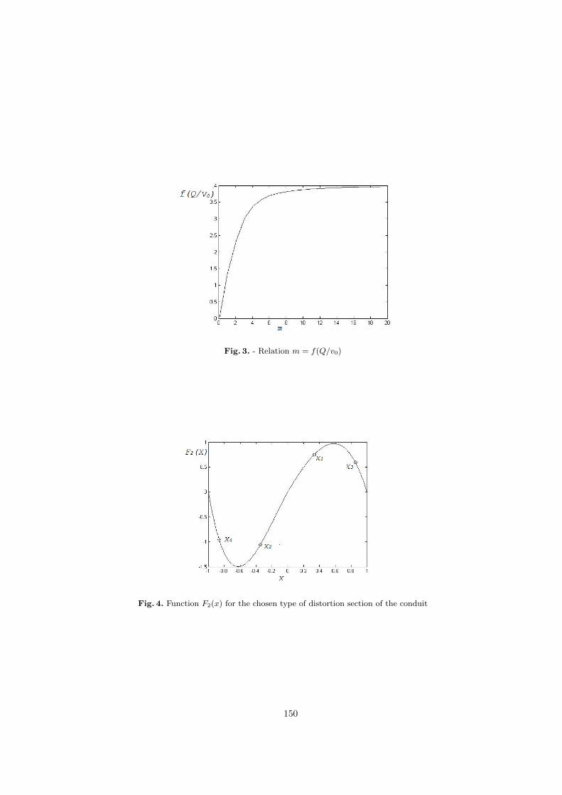
Fig. 3. - Relation m = f(Q/v0)

Fig. 4. Function F2(x) for the chosen type of distortion section of the conduit

150

The calculated values of F1(m,xi), in accordance with (13) and the deter-mined m, are

F1(m,x1) = F1(m,x3) = 1.51; F1(m,x2) = F1(m,x4) = 1.1.

From the estimated value of m F1(m,xi) and by calculation of equations (20)α = 0.26, v0 = 1.16. The error of determination α, v0 obviously connected withaccuracy of estimation m.

The error of recovering the profile of a flow (9) with the calculated values ofparameters and set values estimated as

(1−Qteor

Qcalc

)100% = 6.7%, (21)

whereQteor is the flow rate calculated form the selected valuesm,α, v0, andQcalcis the flow rate calculated from estimated values of parameters. The relation oferror versus the asymmetry coefficient and m = 5, 7, 10 shown in Fig. 5. The

Fig. 5. Relation of error depending on asymmetry coefficient with m = 5, 7, 10 andv0 = 1

accuracy analysis shows that the error dependence has a constant part thatcorresponds to symmetry flow distribution m = f(Q/v0). Such constant value ofthe error can be decreased by correction of calibration relationship m = f(Q/v0).The result with such calibration for each value m is shown in Fig. 6. In the whole,such behavior of the error can be caused by the insufficient accuracy of the modelassumptions. Particularly, it may be supposed that the asymmetry part of F2(x)in (13) is influenced by the symmetry part of F1(x,m).

The general algorithm of flow profile recovering on the basis of multipathultrasonic flow rate measurements and a priori information about distortingfunction of the conduit section has the following stages:

151

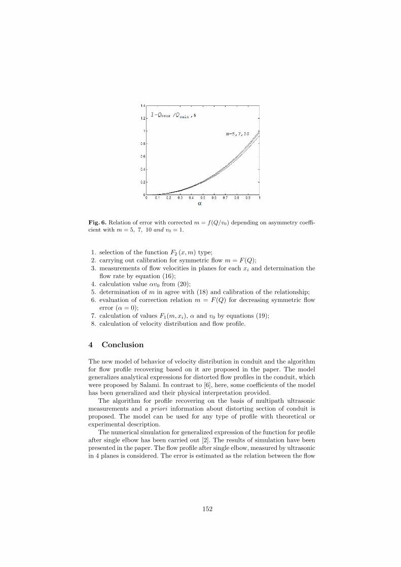
Fig. 6. Relation of error with corrected m = f(Q/v0) depending on asymmetry coeffi-cient with m = 5, 7, 10 and v0 = 1.

1. selection of the function F2 (x,m) type;2. carrying out calibration for symmetric flow m = F (Q);3. measurements of flow velocities in planes for each xi and determination the

flow rate by equation (16);4. calculation value αv0 from (20);5. determination of m in agree with (18) and calibration of the relationship;6. evaluation of correction relation m = F (Q) for decreasing symmetric flow

error (α = 0);7. calculation of values F1(m,xi), α and v0 by equations (19);8. calculation of velocity distribution and flow profile.

4 Conclusion

The new model of behavior of velocity distribution in conduit and the algorithmfor flow profile recovering based on it are proposed in the paper. The modelgeneralizes analytical expressions for distorted flow profiles in the conduit, whichwere proposed by Salami. In contrast to [6], here, some coefficients of the modelhas been generalized and their physical interpretation provided.

The algorithm for profile recovering on the basis of multipath ultrasonicmeasurements and a priori information about distorting section of conduit isproposed. The model can be used for any type of profile with theoretical orexperimental description.

The numerical simulation for generalized expression of the function for profileafter single elbow has been carried out [2]. The results of simulation have beenpresented in the paper. The flow profile after single elbow, measured by ultrasonicin 4 planes is considered. The error is estimated as the relation between the flow

152

rate calculated with theoretical set of parameters and parameters that weredetermined by the proposed algorithm. The obtained accuracy gives less than1% error.

The reached that the model can be considered as reliable. In further devel-opments of the model, the influence of symmetry part of flow on asymmetrypart will be investigated. Moreover, investigation of number of measurementsand orientation of planes influence on accuracy should be done.

References

1. Idelchik, I.E.: Handbook of hydraulic resistance. Mashinostroenie, Moscow (1992)(in Russian)

2. Rychagov, M., Tereshenko, S.: Multipath flowrate measurements of symmetric andasymmetric flows. Invers Problems, 16, 495–504 (2000)

3. Kremlevskij, P.P.: Flowmeters and counters of the amount of substance. Handbook.Politeh, Saint-Peterburg (2004)

4. Brown, G.J., Augenstein, D.R., and Cousins T.: An 8-patch ultrasonic mastermeter for oil custody transfer. XVIII IMEKO WORLD CONGRESS, 17–22 (2006)

5. Rychagov, M.N.: Ultrazvukovye izmereniya potokov v mnogoploskostnyh izmeri-tel’nyh mod-uljah. Akusticheskij zhurnal 44 (6), 829–836 (1998) (in Russian)

6. Salami, L.A.: Application of a computer to asymmetric flow measurement in cir-cular pipes. Trans. Inst. MC. 6(4), 197–206 (1984)

7. Moore, P., Brown and J., Stimpsom, B.: Ultrasonic transit–time flowmeters mod-eled with theoretical velocity profiles: methodology. Meas. Sci. Technol., 11, 1802–1811 (2000)

8. Zheng, D., Zhao, D. and Mei, J.: Improved numerical investigation method forflowrate of ultrasonic flowmeter based on Gauss quadrature for non-ideal flowfields. Flow measurement and Instrumentation. 41, 28-25 (2000)

9. Lui, J., Wang, B., Cui, Y. and Wang, H.: Ultrasonic tomographic velocimeter forvisualization of axial flow fields in pipes. Flow measurement and instrumentation,41, 57-66 (2000)

10. Krylov, V.I.: An approximate calculation of integrals. Nauka, Moscow (1967)

153