Accent Features and Idiodictionariesfaculty.washington.edu/mtjalve/papers/Tjalve07.pdfIn this work,...
237
PhD Dissertation Accent Features and Idiodictionaries: On Improving Accuracy for Accented Speakers in ASR Michael Tjalve Department of Phonetics and Linguistics University College London March 2007
Transcript of Accent Features and Idiodictionariesfaculty.washington.edu/mtjalve/papers/Tjalve07.pdfIn this work,...

PhD Dissertation
Accent Features and Idiodictionaries:
On Improving Accuracy for
Accented Speakers in ASR
Michael Tjalve
Department of Phonetics and Linguistics
University College London
March 2007


ii
Declaration
I, Michael Tjalve, confirm that the work presented in this thesis is my own. Where
information has been derived from other sources, I confirm that this has been
indicated in the thesis.
Copyright
The copyright of this thesis rests with the author and no quotation from it or
information derived from it may be published without the prior written consent of the
author.
2007 Michael Tjalve

iii
ABSTRACT
One of the most widespread approaches to dealing with the problem of accent variation in
ASR has been to choose the most appropriate pronunciation dictionary for the speaker from a
predefined set of dictionaries. This approach is weak in two ways: firstly that accent types are
more numerous and more variable than can be captured in a few dictionaries, even if the
knowledge were available to create them; and secondly, accents vary in the composition and
phonotactics of the phone inventory not just in which phones are used in which word.
In this work, we identify not the speaker's accent, but accent features which allow us
to predict by rule their likely pronunciation of all words in the dictionary. Any given speaker
is associated with a set of accent features, but it is not a requirement that those features
constitute a known accent. We show that by building a pronunciation dictionary for an
individual, an idiodictionary, recognition accuracy can be improved over a system using
standard accent dictionaries.
The idiodictionary approach could be further enhanced by extending the set of phone
models to improve the modelling of phone inventory and variation across accents. However
an extended phoneme set is difficult to build since it requires specially-labelled training
material, where the labelling is sensitive to the speaker's accent. An alternative is to borrow
phone models of a suitable quality from other languages. In this work, we show that this
phonetic fusion of languages can improve the recognition accuracy of the speech of an
unknown accent.
This work has practical application in the construction of speech recognition systems
that adapt to speakers' accents. Since it demonstrates the advantages of treating speakers as
individuals rather than just as members of a group, the work also has potential implications
for how accents are studied in phonetic research generally.

iv
ACKNOWLEDGEMENTS
Many people have contributed to this PhD in many different ways. First and foremost,
I would like to thank my research supervisor Dr. Mark Huckvale for academic
guidance and for many exciting discussions. I have enjoyed how he has challenged
me and my ideas. It has been a privilege to work closely with one of the true experts
in the field of accent variation in speech technology.
I would like to thank Infinitive Speech Systems and Visteon Corporation for
sponsoring my research. The speech data, phonetic data and the speech recogniser
used in the majority of the experiments described on the pages below belong to
Infinitive Speech Systems, and without this agreement, it would not have been
possible to complete the research within the timeframe I had planned.
I would like to thank Dr. Maha Kadirkamanathan, without whom this PhD
would not even have begun. He has been my industrial mentor within speech
technology and he is one of the few persons I have met on the commercial side of the
speech community who truly understands the potential of academia and the industry
working together.
I would also like to thank Darren, Omri, Mark, Paul, Bernard and Gary at
Infinitive Speech Systems for many good discussions, ideas and help.
I am grateful to Dr. Roger Moore for giving me assistance with the Accents of
the British Isles corpus.
Also thanks to Simon King and the Centre of Speech Technology Research at
University of Edinburgh for making the Unisyn dictionary available.

v
Thanks to Mads Torgersen for very valuable proofreading and good
suggestions.
I would like to thank my mother, Merete Tjalve, for always believing in me
and for taking an important part in making me who I am. I would like to thank my
father, Eskild Tjalve, for inspiring scientific thinking and for showing the value of
thinking outside of the box.
Finally, I would like to thank my amazing life companion - my wife Rocío -
and our wonderful children, Isabella and Oliver, for bearing up with me spending time
on this project of mine. It has been a fascinating journey but it has also been a long
one and I could not have done it without your support and understanding. Thank you
for always being there. Jeg elsker jer!

TABLE OF CONTENTS
Abstract .............................................................................................................................. iii
Acknowledgements............................................................................................................ iv
Table of Contents................................................................................................................ 1
1 Introduction .................................................................................................................. 7
1.1 Aims and overview of thesis ................................................................................. 9
1.2 Scope of research................................................................................................. 11
1.3 General notes about the experiments................................................................... 12
1.3.1 The speech data............................................................................................. 12
1.3.2 The ASR engine............................................................................................ 15
1.3.3 The pronunciation dictionary........................................................................ 17
2 Accent Variation and ASR......................................................................................... 19
2.1 Introductory remarks ........................................................................................... 19
2.2 Accent variation................................................................................................... 19
2.3 The mechanics of an ASR engine........................................................................ 24
2.3.1 The acoustic signal........................................................................................ 25
2.3.2 The front-end ................................................................................................ 26
2.3.3 The back-end................................................................................................. 26
2.3.3.1 The acoustic models ...................................................................................26
2.3.3.2 The pronunciation dictionary......................................................................30

2
2.3.3.3 The grammar...............................................................................................31
2.3.4 The response ................................................................................................. 34
2.4 Why accent variation is a problem to ASR engines ............................................ 35
2.5 Summary and discussion ..................................................................................... 36
3 Phonetics and Phonology in ASR .............................................................................. 38
3.1 Introductory remarks ........................................................................................... 38
3.2 Phonetic and phonological variation ................................................................... 39
3.3 Phonetic and phonological representation........................................................... 41
3.3.1 The phoneme set ........................................................................................... 42
3.3.2 The acoustic models...................................................................................... 44
3.3.3 The pronunciation dictionary........................................................................ 46
3.4 Summary and discussion ..................................................................................... 47
4 Accent Variation Modelling....................................................................................... 49
4.1 Introductory remarks ........................................................................................... 49
4.2 The acoustic models ............................................................................................ 50
4.2.1 Training of the acoustic models.................................................................... 51
4.2.1.1 Details of the experiment............................................................................52
4.2.1.2 Findings ......................................................................................................53
4.2.2 Speaker adaptation of the acoustic models ................................................... 54
4.2.2.1 Details of the experiment............................................................................57
4.2.2.2 Findings ......................................................................................................58
4.3 The pronunciation dictionary............................................................................... 60
4.3.1 The canonical dictionary............................................................................... 60
4.3.2 The multiple pronunciations dictionary ........................................................ 61

3
4.3.2.1 Details of the experiment............................................................................62
4.3.2.2 Findings ......................................................................................................62
4.3.3 The Oracle dictionary ................................................................................... 64
4.3.3.1 Details of the experiment............................................................................65
4.3.3.2 Findings ......................................................................................................65
4.4 Accent Identification ........................................................................................... 66
4.4.1 Non-native accented speech.......................................................................... 67
4.4.2 Native accented speech ................................................................................. 70
4.4.3 Accent identification accuracy...................................................................... 74
4.4.4 Defining accent groups ................................................................................. 75
4.4.5 Accent dictionary adaptation ........................................................................ 77
4.4.5.1 Details of the experiment............................................................................77
4.4.5.2 Findings ......................................................................................................79
4.5 Summary and conclusion..................................................................................... 81
5 Pronunciation Dictionary Adaptation......................................................................... 83
5.1 Accent features .................................................................................................... 83
5.2 Idiodictionaries .................................................................................................... 88
5.2.1 Details of the experiment.............................................................................. 91
5.2.2 Findings......................................................................................................... 94
5.3 SA of test dictionary using various numbers of utterances ................................. 97
5.3.1 Details of the experiment.............................................................................. 97
5.3.2 Findings......................................................................................................... 97
5.4 SA of the training dictionary ............................................................................... 99
5.4.1 Details of the experiment.............................................................................. 99

4
5.4.2 Findings....................................................................................................... 100
5.5 SA of the training and the test dictionaries........................................................ 101
5.5.1 Details of the experiment............................................................................ 101
5.5.2 Findings....................................................................................................... 102
5.6 Probability-based selection of accent features................................................... 103
5.6.1 Details of the experiment............................................................................ 104
5.6.2 Findings....................................................................................................... 110
5.7 Summary and discussion ................................................................................... 111
6 Phonetic fusion......................................................................................................... 113
6.1 Lack of speech data ........................................................................................... 113
6.2 Acoustic models trained with small amounts of data ........................................ 116
6.2.1 Details of the experiment............................................................................ 117
6.2.2 Findings....................................................................................................... 118
6.3 Introducing phonetic fusion............................................................................... 118
6.3.1 Uniphone..................................................................................................... 119
6.3.2 How it works............................................................................................... 121
6.3.3 Benefits and limitations .............................................................................. 122
6.4 Building a new speech recogniser ..................................................................... 123
6.4.1 Illustration of methodology......................................................................... 124
6.4.2 Missing phonemes and acoustic proximity................................................. 125
6.4.3 Details of the experiment............................................................................ 127
6.4.4 Findings....................................................................................................... 127
6.5 Phonetic fusion by language family .................................................................. 128
6.5.1 Germanic training data................................................................................ 129
5
6.5.2 Romance training data ................................................................................ 130
6.5.3 Findings....................................................................................................... 130
6.6 Gradual addition of Italian speakers.................................................................. 132
6.6.1 Details of the experiment............................................................................ 133
6.6.2 Findings....................................................................................................... 133
6.7 Multilingual speech recognition ........................................................................ 136
6.7.1 Details of the experiment............................................................................ 136
6.7.2 Findings....................................................................................................... 137
6.8 Non-native speech recognition .......................................................................... 138
6.8.1 Details of the experiment............................................................................ 140
6.8.2 Findings....................................................................................................... 141
6.9 Targeted phone modelling ................................................................................. 142
6.9.1 Details of the experiment............................................................................ 143
6.9.2 Findings....................................................................................................... 145
6.10 Summary and discussion ................................................................................... 146
7 Putting it all together................................................................................................ 147
7.1 Evaluation of previous experiments .................................................................. 147
7.2 Idiodictionaries and SA of the acoustic models ................................................ 147
7.2.1 Details of the experiment............................................................................ 148
7.2.2 Findings....................................................................................................... 148
7.3 Idiodictionaries and targeted phone modelling ................................................. 150
7.3.1 Details of the experiment............................................................................ 150
7.3.2 Findings....................................................................................................... 151
7.4 Everything combined......................................................................................... 152

6
7.4.1 Details of the experiment............................................................................ 153
7.4.2 Findings....................................................................................................... 153
7.5 Summary and discussion ................................................................................... 154
8 Discussion and Conclusion ...................................................................................... 156
8.1 Summary and discussion ................................................................................... 156
8.2 Thesis contributions........................................................................................... 157
8.3 Future research .................................................................................................. 159
8.3.1 Enhancements of the accent feature approach ............................................ 159
8.3.2 Second language learning ........................................................................... 161
8.3.3 Sociolinguistic studies ................................................................................ 162
8.4 Conclusion......................................................................................................... 162
9 References ................................................................................................................ 164
10 Appendix .................................................................................................................. 173
10.1 Index of figures and tables................................................................................. 173
10.2 British English Phoneme set.............................................................................. 175
10.3 Speech data for experiments.............................................................................. 180
10.3.1 Speaker adaptation set................................................................................. 180
10.3.2 Test set ........................................................................................................ 181
10.4 Pronunciation dictionary with accent features................................................... 187
10.5 List of publications ............................................................................................ 229

7
1 INTRODUCTION
Automatic Speech Recognition (ASR) is a technology which allows a person to control a
device entirely by voice. ASR combines many disciplines. Creating a successful ASR
engine takes experts from as diverse fields as acoustics, linguistics, psychology, computer
science, electrical engineering and mathematics. Optimising one component of the speech
engine may have a negative impact on other components, and it is therefore important to
know the engine as a whole.
With the exception of dictation software, speech recognisers are relatively futile
by themselves. They merely convert the speech signal into either a string of phonemes or
a string of words. Although that itself is a very complex process, it is not until the ASR
engine is combined with other components in an application that it becomes capable of
having a direct impact on the outside world. However, when this is achieved, ASR
becomes a very powerful and attractive means of interaction. As an enabling technology,
ASR has taken a key role in automotive applications (hands-free dialling and control of
centre stack functionalities like music, climate control and navigation), cell phone
applications (server-based or directly on the handset), PC applications (dictation, voice
control of other PC software) and elsewhere. It has an obvious value as a commodity
provider but it is also capable of filling actual needs e.g. by enabling physically impaired
to use computers.
Speech is the most natural interface in human-to-human communication. It
therefore makes sense to make speech the focal point in Human-to-Machine Interfaces
(HMI). However, the natural feel to a speech-enabled HMI is only fully achieved when
the application allows the user to intuitively interact with the system in the same way
8
he/she would with another person. Human-beings are able to understand conversational
speech by filtering out redundant input like auto-corrections, hesitation and stuttered
speech. We can handle recognition errors by considering the context of the conversation.
As listeners, we adapt to the speech situation thus minimising the negative impact of
environment noise and pronunciation variation. All these factors facilitate communication
and allow people to speak naturally. The ideal speech application should be able to mimic
this behaviour and in the current work we shall attempt to provide a tool which can take
us one step further in that direction.
However, speech technology has traditionally had a bad reputation since it was
first made commercially available to the general public in the 1980s. The frustration of
having to talk to the recogniser exactly the way it expects you to has often been expressed
by end-users. Although many advances have been achieved within the field of speech
recognition, most ASR engines still remain very fragile when exposed to variation in the
acoustic input. The speech community could therefore benefit from developing more
flexible speech engines capable of adapting to the user rather than expecting that the user
will effortlessly adapt to the engine. By improving on this flexibility, we can enhance the
user experience and achieve greater acceptance of speech technology by the general
public.
The performance of speech engines is challenged by various outside factors.
Speech recognition in noisy environments is compromised by the unclean acoustic signal.
Spontaneous speech is difficult to deal with due to phenomena like hesitation, auto-
correction and unexpected word combinations. Pronunciation variation - and in particular
accent variation - is also considered by many researchers to be one of the greatest
challenges in ASR today. In Humphries et al. (1996), for example, accented speakers are
9
tested on a canonical1 speech recogniser. Their recognition accuracy is 20% lower on the
canonical speech recogniser compared with when the recogniser is adjusted to their
accent. Many researchers report similar degradation when there is a mismatch between
the accent of the training speakers and the accent of the test speakers (see e.g. Strik and
Cucchiarini (1999), Diakoloukas et al. (1997), Barry et al. (1989), Beringer et al. (1998),
Huang et al. (2001)). As speech technology software is made available to more people
and it is being used for more diverse purposes2, ASR engines are exposed to an
increasing amount of accent variation and it is therefore vital that we as speech
researchers develop efficient techniques for handling this variation. Accent variation
modelling tries to do exactly that and in the current work, we shall analyse the existing
research in this area as well as explore the possibility of making new contributions to the
speech community within accent variation modelling.
1.1 Aims and overview of thesis
Accent variation modelling in ASR is a fascinating area of research which encompasses
many challenges. The aims of the current work are:
• To understand why accent variation is a problem in ASR
• To become familiar with the existing research within accent variation modelling
• To create an experimental setup in order to study the problem in detail at first
hand
1 For a discussion on the canonical form, see Sections 2.2 and 4.3.1 below. 2 In fact, part of the current dissertation was written using dictation software and a text-to-speech
engine was used on several occasions to read out the contents of the chapters.

10
• To evaluate experimental results and identify possible improvements
• To learn more about the nature of accent variation
• To learn more about how accent variation can be modelled in such a way that the
knowledge is useful in ASR
• To develop and implement alternative approaches and compare with existing ones
These aims will be explored in the following chapters. In Chapter 2, we will first
try to define what accent variation is. Then we will look at the various components of a
typical ASR engine and try to explain why accent variation is a challenge to speech
recognisers. In Chapter 3, we will present a discussion about the differences between
phonetic and phonological information in the context of ASR in an attempt to better
understand the consequences of our decisions. In Chapter 4, we will investigate the
existing literature and research within accent variation modelling. We will reproduce
some of the traditional approaches to dealing with accent variation in ASR in order to
establish benchmark experiments. In Chapter 5, we will present a novel technique to
modelling accent variation at the pronunciation dictionary level. In Chapter 6, we will
demonstrate the benefit of including speech data from multiple languages during training
for accent variation modelling. In Chapter 7, we will combine the most successful
approaches investigated in the current work in an attempt to obtain further improvements.
In Chapter 8, we will conclude the thesis by summarising our work and findings and by
suggesting future research.

11
1.2 Scope of research
In this section, we shall specify the scope of the research presented in the current work.
Unless otherwise specified, the experiments described in the subsequent chapters follow
the limitations laid out in this section.
The pronunciation of a given word can differ from speaker to speaker according
to a number of factors. Aspects such as gender, age, size, emotional state, physical state,
speaking style as well as regional background all have an impact on the acoustic
realisation of speech. The methodology presented in the current work is designed to be
applied on any type of pronunciation variation which can be consistently described by a
phonetic representation. This potentially includes phenomena such as rapid speech,
disfluency and speech impairment. In the current work, we have chosen accent variation
as our domain of primary interest for investigation and validation of the methodology.
Accent variation follows certain relatively consistent patterns. The challenge in
accent variation modelling is to identify those patterns and to implement this information
into the ASR engine in order to improve recognition of accented speech.
We have chosen to focus our research on native accented speech in order to limit
the set of variables. The pronunciation patterns of non-native accented speech depend on
factors like level of proficiency and similarity between native language and target
language and describing this variability easily becomes unmanageable especially if the
native language is unknown. Moreover, most ASR applications are created for native
speakers. However, in Section 6.8 we have included one experiment with non-native
speech for validation of the methodology.
The geographical area of research described in the current work is limited to focus
on the British Isles and we work with the many diverse accents of British English. British

12
English accents were chosen because they are exhaustively described in the literature.
Unless otherwise specified, all examples of phonemes, phonetic features, accents and
more refer to British English.
Recognition of large vocabularies and in particular Large Vocabulary Continuous
Speech Recognition is a great challenge regardless of accent variation. However, that is
not a problem we shall attempt to solve in the current work. Instead, we chose to design
our experiments with a limited vocabulary and a command and control grammar in order
to isolate the impact of accent variation and of accent variation modelling. This also
means that we choose to ignore the differences in vocabulary which may exist between
accents.
We shall explore the existing approaches to accent variation modelling and
investigate how much improvement they obtain. We will then analyse the advantages and
shortcomings of each approach and, based on our findings, attempt to develop a new
approach. We hope that this new approach will reach new levels of improved recognition
accuracy of accented speakers and that it can potentially be combined with existing
approaches.
1.3 General notes about the experiments
1.3.1 The speech data
The key experiments reported in the current work were carried out on British English
speech data. Unless otherwise specified, the following data sets were used in the

13
experiments. Two separate data sources were chosen to avoid the training data
influencing the test data and the following three data sets were defined:
• Training set:
o 247 speakers, 69,615 utterances
o Commands and phonetically rich sentences
o Collected at Dragon Systems
• Adaptation set:
o 158 speakers, 25 phonetically rich sentences per speaker
o Extracted from the shortsentences and shortphrases of the ABI corpus
• Test set:
o 158 speakers, 100 sentences per speaker
o Extracted from the catalogue codes, equipment control, game commands
and PIN numbers of the ABI corpus
The actual sentences from the speaker adaptation and the test set can be seen in
Section 10.3 in the Appendix. The training set cannot be shared as it is commercial-in-
confidence. This corpus was collected to build the British English speech engine at
Dragon Systems. This data is now owned, maintained and applied in speech applications
by Infinitive Speech Systems. The recordings were collected in a stationary car
environment using a close-talking microphone. The speakers are amateur speakers
considered to be representative of the typical end-user of automotive speech applications.
There is approximately a 50/50 split between female and male speakers and the age of the

14
speakers range from 18-60. The training data contains recordings from the following
broad accent regions:
• Northern England
• Scotland
• Ireland
• Wales
• South-West England
• South-East England
• Received Pronunciation
In this data collection, Received Pronunciation (RP) is not defined as representing
any particular region.
The Accents of the British Isles (ABI) corpus is ideal for accent variation
research. This corpus was collected by the University of Birmingham in association with
Aurix. With its speech data from 14 accent regions from all around the British Isles, it
offers a very comprehensive coverage of British English accent variation. Data from the
following accent regions were used in the experiments:
• Belfast, Northern Ireland
• Birmingham
• Burnley, Lancashire
• Denbigh, North Wales
• Dublin, South Ireland

15
• Elgin, Scottish Highlands
• Glasgow, Scotland
• Hull, East Yorkshire
• Liverpool
• Lowestoft, East Anglia
• Newcastle
• Standard British English
• Tower Hamlets, Inner London
• Truro, Cornwall
The adaptation set consists of the “short sentences” and the “short phrases” from
the ABI corpus. In order to keep the recognition task relatively simple, we built a test
grammar which distinguishes between entire phrases rather than single words. For this
reason, the results in this paper are presented as sentence error rates (SER) instead of
word error rates. The test grammar consists of the “catalogue codes”, the “careful words”,
the “equipment control” commands, and the “PIN numbers” from the ABI corpus.
An extension to the ABI corpus, called ABI-2, is now available through The
SpeechArk (www.thespeechark.com). It contains 13 new accents regions which were not
available in the original ABI corpus.
1.3.2 The ASR engine
Two ASR engines were used in the experiments presented in the current work. The first
one is called CREC. It was developed at Dragon Systems and it is now owned and further
developed at Infinitive Speech Systems in the UK. The details of the engine described
16
here are presented as commercial in confidence. CREC was configured with 36
parameters: 12-MFCC including C0 + deltas + delta-deltas. Linear discriminant analysis
(LDA) was performed resulting in an IMELDA transform (linear) being applied to 36
dimensional vector to create LDA parameters. The HMMs trained with CREC for the
experiments were trained as phones-in-context (PICs) where each phone is considered in
the context of the left and the right neighbouring phone. The HMMs mostly consisted of
two states, with a few phonemes acoustically complex phonemes, e.g. diphthongs and
affricates, having three states. A maximum of 6 Gaussians per mixture was allowed
during the training process. The Gaussians were clustered based on context, driven by a
decision tree clustering methodology. No state skipping was allowed either during
training or decoding. The Viterbi decoder applied full cross-word contexts during the
search. An approximate duration probability model was also applied during the
computation process. In addition to the phone models described in Section 10.2 for
British English, a phone model for silence was trained.
For one experiment3, though, HTK version 3.2 (see Young et al. (2002)) was used
instead because this engine has the capability to include probability weightings for
individual pronunciations in the pronunciation dictionary. The HMMs were trained on the
WSJCAM0 corpus (see Fransen et al. (1994)) using 100 sentences from each of the 50
training speakers. It was configured with 39 parameters: 12-MFCC + energy + deltas +
delta-deltas. The HMMs were trained as 10,000 PICs without state skipping and with 8
Gaussian mixtures per state. Model-level clustering was performed using a decision tree
system. There were 45 symbols in the phoneme set.
3 See Section 5.6
17
1.3.3 The pronunciation dictionary
The pronunciation dictionaries used for training the acoustic models were developed at
Infinitive Speech Systems and due to the commercially sensitive nature, the content
cannot be shared in the current work. The phoneme set used in these dictionaries is
Uniphone which is described in Section 6.3.1 below.
The pronunciation dictionaries used during recognition, on the other hand, are
derived from the Keyword Lexicon (see Fitt (1997), Williams and Isard (1997), Fitt and
Isard (1999), and more recently Bael and King (2003)). The Keyword Lexicon was
created as part of the UniSyn project4 at the Centre of Speech Technology Research
(CSTR) at University of Edinburgh with the purpose of having a single universal source
of pronunciations for creating TTS in different accents. It contains a very large amount of
words, close to 120,000, and an extensive coverage of pronunciation variants. The idea
behind the Keyword Lexicon builds on Wells’ standard lexical set (Wells (1982)), where
the behaviour of a phoneme across accents is characterised by a class of words exhibiting
the same behaviour. Apart from containing an exhaustive coverage of common
vocabulary, the main benefit of this pronunciation dictionary is the flexibility it offers. As
an abstract dictionary it allows the user to extract specific pronunciations and thus build
accent-specific dictionaries. In order to capture all the variation in British English, the
Keyword Lexicon is based on a very large phoneme set of 83 phonemes. The dictionary
comes with a set of tools to create pronunciation variants reflecting various accent
regions. We chose the following five major accent regions and extracted pronunciations
representing those accents:

18
• Ireland
• Scotland
• Wales
• North-England
• South-England
For the experiments in Chapter 6 where speech data from languages other than
English were used, the pronunciation dictionaries were derived from the Infinitive Speech
Systems phonetic database.
4 See http://www.cstr.ed.ac.uk/projects/unisyn
2 ACCENT VARIATION AND ASR
2.1 Introductory remarks
Accent variation is generally considered to be one of the biggest challenges in ASR
today (see e.g. Kessens et al. (2002), Strik and Cucchiarini (1999), Arslan and Hansen
(1996), Vaseghi et al. (2003)). The first step to solving any problem is to understand
why the problem arises. In this chapter, we will therefore investigate why accent
variation is a problem to ASR engines. We shall first attempt to identify and describe
the characteristics of accent variation in the context of ASR. This exercise will
include the definition of accent variation as it is used in the current work. Then we
will look at the components of a typical ASR engine and how they relate to each
other. This discussion will help us understand why accent variation is a problem in
ASR.
2.2 Accent variation
There is a great deal of variability in the way people speak. Pronunciation variation is
due to many factors such as emotional and physical state as well as differences in size,
gender and age. Pronunciation variation is also influenced by the geographical area in
which the speaker grows up and lives as well as by factors such as social class,
cultural background, education and job environment. All of these factors have an
impact on the conditions for speech recognition, both human speech recognition and

20
automatic speech recognition. Some parts of this pronunciation variation are
consistent over time whereas others may change or be adapted to the speaking
environment.
Pronunciation variation can happen at the lexical, grammatical, phonetic,
phonological and prosodic levels. However, here we are only concerned with phonetic
and phonological variation1 and we shall refer to this type of variation as accent
variation.
In ASR, it is common to consider accent variation in relation to a canonical
pronunciation (Humphries et al. (1996), Huang et al. (2000)). The canonical
pronunciation in ASR is most often defined as the statistically most representative
variant (Fukada et al. (1999), Kessens (2002)) and the other pronunciation variants of
a word can thus be considered accent variation2. The rationale behind this approach is
that it is statistically possible to cover the majority of occurrences of a given word
with merely one pronunciation which keeps the size and complexity of the
pronunciation dictionary to a minimum. The canonical pronunciation in terms of ASR
does thus not necessarily refer to any known accent and whereas the definition and
application of a canonical pronunciation may not make much sense in traditional
linguistic terms, it does provide benefits in the realm of ASR. See Section 4.3.1 for
further discussion about the canonical dictionary.
Research in accent variation in ASR most often focuses on differences
between regional groups of people. The speakers’ accents are categorised according to
1 For a definition of phonetic and phonological variation, see Chapter 3. 2 With the exception of context-dependent pronunciation variants like “the” in “the apple”
versus “the pear” as well as elisions due to fast speech.

21
their geographical affiliation, e.g. Yorkshire accent versus Southern English accent3.
Following this tradition, we can define accent variation as
Differences in pronunciation patterns shared by groups of people within a
linguistic area due to regional influences
In this definition, the phrases groups of people and due to regional differences
make reference to how speakers are divided into groups according to the accent
spoken in a specific region. The term linguistic area emphasises on the fact that we
are dealing with variation within one language only, thus excluding non-native
accented speech4. According to this definition, we can consider that
accent = regional accent
Many ASR researchers have successfully based their work on this definition in
an attempt to improve recognition accuracy for accented speech. The perhaps most
popular approach has been to define a number of accent groups and assign each of
these a corresponding pronunciation dictionary. The challenge is then to identify the
accent group of the speaker after which the best matching pronunciation dictionary
can be loaded. This discipline is called accent identification and is described in detail
in Section 4.4 below.
3 See section 4.4.5. 4 For a discussion on non-native accented speech, see Section 4.4.1 below.

22
Predefined accent groups can offer some level of solution to the problem of
accent variation. However, accents are not as homogeneous as we often consider them
to be5. If the accent groups are defined according to geographical or cultural criteria
rather than on the basis of phonological and phonetic similarity, many speakers will
not fit in well. Not all speakers in Scotland correspond to the Scottish accent. The
Scottish accent has certain characteristics, but it does not mean that everybody in
Scotland speaks with an accent that has all of these characteristics and it does not
mean that somebody outside of Scotland cannot speak with some or all of these
characteristics.
Moreover, in ASR we are not recognising groups of speakers. We are only
recognising one speaker at a time. If we set up our ASR system to treat speakers as
part of a predefined geographical group, we exclude ourselves from accessing a great
deal of detail regarding each speaker’s accent. In the context of ASR, we could
therefore benefit from making a distinction between accent and regional accent and
work with a more fine-grained description. In the current work, we shall consider that
accent ≠ regional accent
To talk about e.g. a northern accent makes sense when describing trends
within a specific region, but in the context of accent variation in ASR, we abandon the
notion of regional accent and consider accent as something individual to each speaker.
This brings us to the following definition of accent
5 See discussion of Barry et al. (1989) in Section 4.4.2 below.
23
Differences in pronunciation patterns between individual speakers within a
linguistic area due to regional influences
In this definition, the phrase individual speakers refers to the fact that we do
not try to fit speakers into predefined regional groups. The phrase due to regional
influences describes the fact that any speaker’s accent may have been influenced by
any number of regional characteristics. People move around between regions now
more than ever. This trend exposes cultural, social and regional pronunciation
variation to both the people who move and to the people in the regions to which they
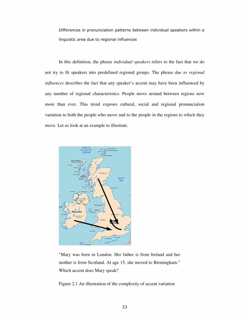
move. Let us look at an example to illustrate.
"Mary was born in London. Her father is from Ireland and her
mother is from Scotland. At age 15, she moved to Birmingham.”
Which accent does Mary speak?
Figure 2.1 An illustration of the complexity of accent variation

24
The example illustrated in Figure 2.1 above is admittedly a rather extreme
case of regional influences, but many speakers are familiar with one or more of these
conditions and it is clear that the notion of regional accent fails to describe her accent
exhaustively. The question then is: how does this impact the ASR engine? In the next
sections, we shall look at the components of an ASR engine and how accent variation
impacts speech recognition.
2.3 The mechanics of an ASR engine
We have now been introduced to the concept of accent variation. In this section, we
shall look at the various components of a typical ASR engine and, based on what we
saw in the previous section and what we learn in this section, we shall attempt to
explain why accent variation causes problems to the ASR engine.
There are various approaches to building an ASR engine and not all
components are present in all speech recognisers. On the pages below, we shall
describe the most typical components of an ASR engine as well as their functions and
how they work together.
Figure 2.2 shows the major components of such an ASR engine. The first box
(acoustic signal) and the last box (response) are not part of the ASR engine as such,
but they have been included in this figure to illustrate the recognition cycle from
beginning to end. The response box is the component that allows the ASR engine to
reach out to the real world and make a tangible change.

25
Figure 2.2 Overview of the main components of a typical ASR engine
For details about the ASR engines used in the current work, see Section 1.3.2.
2.3.1 The acoustic signal
Under ideal conditions, the most significant part of the acoustic signal is just the
speech of the person using the system. The user says a command or a phrase that
she/he wants the system to understand. In the ideal scenario, the speech signal is
clean, well-articulated and relevant. However, this is far from always the case and this
is one of the reasons that ASR engines often struggle with understanding what is said.
Depending on where the speech application is used, there may be extraneous speech
in the acoustic signal, e.g. other people than the user talking, or the acoustic signal
may contain a variety of non-speech information, e.g. environmental noise. This
further complicates the ASR task. We shall see how this can be dealt with in the
section about acoustic models below.

26
2.3.2 The front-end
The front-end is the part of the ASR engine that converts the acoustic signal into a
time-based sequence of feature vectors. This process is called feature extraction and
the first step is to divide the speech signal into very short (typically 10-30ms)
overlapping frames. By analysing each frame, the engine can gather information
about the acoustic properties of the speech signal relevant to the identification of
words. Typically, speech recognition is based on a multidimensional representation of
the spectral envelope. By normalising the frames, it is possible to accommodate some
variation in acoustic signal such as background noise.
2.3.3 The back-end
The back-end of the speech engine analyses the acoustic features extracted from the
front-end process and attempts to come up with a hypothesis about what was said.
This is known as the search process. The various components and processes in the
back-end box shown in Figure 2.2 are described in this section.
2.3.3.1 The acoustic models
Prior to recognition, a set of acoustic models are trained on a large amount of speech
data of known utterances. These acoustic models contain information about the
characteristics of the acoustic signal that the speech engine is able to recognise.
Differences in the length and shape of the vocal tract are materialised in the speech as
acoustic differences. Speech data from many speakers are included in the training

27
process to ensure a representative coverage of these speaker characteristics. In Section
4.2, we shall look closer at this.
By including speech data from various accents, the acoustic models are to
some degree capable of implicitly model accent variation. The word “cup” can for
example be included in the training data to train a phone model for the vowel /ʌ/.
However, if some training speakers pronounce “cup” as [kʌp] whereas others
pronounce it as [kʊp], the phone model for /ʌ/ becomes in theory capable of
handling both variants. In Section 4.2.1, we shall see an experiment where this
approach is applied for recognition of speakers of various accents.
A widespread approach to acoustic modelling is to train Hidden Markov
Models (HMMs) for a set of phonetic units. HMMs are a type of statistical model
used to represent the sequence and variation of acoustic features extracted in the
front-end process for a single unit of recognition. Each phoneme defined in the
phoneme set for the language in question is represented by one or more HMMs
containing details about the distribution of the acoustic parameters for that specific
phoneme. For robustness, many engines also train acoustic models for silence and
non-speech noise.
Figure 2.3 shows state transitions within HMMs. It is possible to loop within
the same phoneme for several states. Typically, each phone is modelled with three
states and transitions connecting them.

28
Figure 2.3 HMMs showing phone-level state transitions
Alternatively, the number of states for each phone may vary according to their
acoustic complexity, i.e. diphthongs and affricates may last more states than
monophthongs and fricatives respectively.
The phones can be modelled as either independent or dependent of the
surrounding phones. When they are modelled independent of the context, they are
called context-independent phones or simply monophones. When the context in which
they occur is included, they are often called context-dependent phone models. In the
experiments presented in this work, each phone is modelled in the context of its left
and right neighbouring phone. This type of model is often called a triphone, but since
this term is fairly misleading (it suggests that it is a cluster of three phones) we shall
instead refer to them as phones-in-context (PICs). Since PICs are considering the
context of each phone, one has to train significantly more PICs than monophones with
the same speech data. The PICs needed to model the canonical pronunciation of the
word “singing” are:
s(SIL,I), I(s,N), N(I,I), I(N,N), N(I,SIL)

29
where “s(SIL,I)” is read as “/s/ in the context of /SIL/ and /I/”. The phone /SIL/
represents silence before and after the word. We can see that we need two distinct
PICs to model the two contexts in which the phone /I/ appears. When building
monophones for the same word, we can cover the two occurrences of the phone /I/
with just one acoustic model. The monophones needed for the same word are:
s, I, N
So, which of the two phone model types is the best? There is no one true
answer to this question. It depends on the training data and the application. PICs
provide a more restricting search than monophones by disallowing certain phone
combinations. In addition, monophones have larger variance because of contextual
influence from adjacent phones, whereas PICs are less variable in nature. On the other
hand, PICs require more training data since there are significantly more models to
train. This larger model set also consumes more memory in the application. If only
small amounts of training data are available, building monophones is often the better
choice. However, when a sufficient amount of training data is available and if the
added memory consumption is within the acceptable limit, speech scientists tend to
prefer to train PICs because they give better accuracy than monophones.
The acoustic models, once they have been defined and trained, play a key role
in the search process. The acoustic features extracted in the front-end process are
compared against the acoustic models and a series of hypotheses are generated as the
search moves along in time frame by frame. For each frame, the most likely HMM is
identified. The HMMs function as a mapping between the acoustic signal and the

30
phonemes. The phonemes in turn map to words in the dictionary and the words map
to sentences in the grammar. The recognition result is typically given as the sentence
with the greatest likelihood given the input and the model.
As we saw above, the acoustic models are to some degree capable of
modelling speaker variation. This can be further optimised to the individual speaker
by performing Speaker Adaptation (SA) of the acoustic models where the acoustic
models are adapted to the physiological and phonetic characteristics of the speaker. In
Section 4.2.2, we shall explore the potential and limitations of this approach.
2.3.3.2 The pronunciation dictionary
The pronunciation dictionary contains a list of words. Each word is followed by a
phonemic transcription, i.e. a sequence of phonemes. The function of the phonemic
transcription is to describe how the word is pronounced, or rather how it is expected
to be pronounced. Often, there is more than one possible pronunciation for a given
word and alternative pronunciations may be included in the pronunciation dictionary.
For the word “bath”, for example, the pronunciation dictionary can contain both the
pronunciation [bɑ:θ] and the pronunciation [bæθ]. This means that phonological and
phonetic differences between speakers can be covered within the pronunciation
dictionary. There is potential benefit of adding pronunciation variants to the
pronunciation dictionary. However, there is also an increased risk of confusion
between entries when the pronunciation dictionary contains multiple pronunciations
for each word. In Section 4.3.2, we shall look at the benefits and risks of working with
multiple pronunciations.

31
The pronunciation dictionary is used during two different phases in the ASR
engine: during training of the acoustic models and during recognition. During
training, the pronunciation dictionary provides information about which phones to
model for the words in the training data. The training data usually consist of a)
phonetically rich utterances which are chosen to ensure a broad phonetic coverage for
general robustness of the acoustic models and to deal with unknown words, and b)
application targeted utterances which are chosen to boost recognition of specific
words available during recognition. The recognition dictionary contains phonemic
transcriptions for the supported vocabulary. It functions as the link between the
acoustic models and the supported vocabulary.
The same pronunciation dictionary can be used for monophones and PICs. The
word-level identification is combined with the grammar which contains information
about allowed combinations of words.
2.3.3.3 The grammar
The ASR grammar defines the supported vocabulary and it impacts the HMM-level
search by constraining the order in which the words can be successfully uttered. The
grammar provides structure to the recognition process by constraining the search. The
complexity of the ASR grammar can vary tremendously depending on the needs
imposed by the application. An ASR grammar can be as simple as to exclusively
define the option between e.g. “up” and “down”. Figure 2.4, illustrates a grammar of
this type.

32
Figure 2.4 Basic ASR grammar
The speech signal has to be able to be mapped to a valid grammar path for the
utterance to be accepted by the ASR engine. Given the speech input, the ASR will
either go down a valid grammar path and return the recognition result or, if no
hypothesis was confidently identified, it will reject the utterance. For such a grammar,
provided that all other components work well, the average recognition accuracy
should be very close to 100%. As the complexity of the grammar increases, accuracy
is expected to drop. The complexity can be due to the addition of multifaceted
grammar paths defining valid word sequences or simply due to the inclusion of a very
large flat list of items at one node as e.g. street names. Combining those two factors,
i.e. complex grammar paths and a large vocabulary provides a very challenging
recognition task. An example of this is Large Vocabulary Continuous Speech
Recognition (LVCSR) or dictation. If an LVCSR application is created by simply
adding all the supported paths to the grammar, recognition accuracy is likely to be
very low. A language model is therefore often created instead of a simple ASR
grammar. A language model contains information about all the likely grammar paths
and one could consider an ASR grammar to be a very basic form of a language model.
In addition to the information about likely grammar paths, the language model

33
typically contains information about weighting of specific transitions within an n-
gram model. Most often, this is defined as a trigram grammar as shown in Figure 2.5,
where weighting is added to the grammar for improved recognition accuracy.
Figure 2.5 ASR grammar with weighting
The information about weighting can be added to the grammar manually, but
with a large grammar this quickly becomes an overwhelming task. An alternative to
this approach is to use a Statistical Language Model (SLM) instead. SLMs are trained
on large amounts of text data capturing statistical data about prior probabilities based
on how frequent each word occurs and conditional probabilities which take into
consideration the context in which each word occurs thereby modelling transition
patterns. This information is stored within the SLM and it offers a probabilistic
approach to word-level recognition.
All the steps described above take an active part in the recognition process and
the information gathered at each step is taken into consideration to identify the most
likely recognition result. The recognition result can be given as the best scoring single

34
hypothesis or as an n-best list of the best hypotheses. When the speech signal has
successfully been mapped to one or more valid grammar paths, it is up to the
application to decide what to do with it. The grammar should therefore only provide
results which the application can understand. Moreover, it typically makes sense to set
a minimum threshold for the confidence score of the recognition result. If the score is
below the threshold, the application may be told that the utterance was rejected and
the application can then offer help, e.g. simply by asking the user to try again. Setting
a threshold for the confidence score improves the likelihood that what is given by the
ASR to the application is actually what the user intended to say.
2.3.4 The response
As mentioned above, the response is not part of the ASR engine as such. However,
when the recognition result is converted into a response, it is possible for the ASR
engine to have a direct impact on the outside world. The response can be feedback,
e.g. visual display or a voice prompt, or it can be an action like changing the radio
channel. In a dictation application, the recognition result itself is the end goal, and it is
passed on as such to the document. The response also makes it possible to keep a
dialogue going between the user and the application. The user may be invited to speak
again after the response and the recognition cycle can thus start over again.
If the ASR engine completely fails to recognise a spoken utterance, a voice
prompt can inform the user by saying something like “I didn’t understand you. Please
try again”. If the two highest scoring recognition hypotheses are close, the response
may be something like “Did you mean <A> or <B>?”

35
2.4 Why accent variation is a problem to ASR engines
The condition for achieving high recognition accuracy is maximised when the speech
input closely matches the model assumptions. Deterioration of accuracy is therefore
due to a less than optimal match between what the ASR engine is expecting and the
acoustic signal6. The acoustic signal is the primary source
7 for recognition
hypotheses. If the acoustic signal deviates from the model assumptions, the conditions
for making hypotheses are compromised. The ASR engine will still try to find a
match, but it will then be more likely that the best match is incorrect. If for example
the noise condition in the training data is different from the noise condition at
recognition time, it may be difficult to identify a reliable acoustic match. Another
example is pronunciation variation due to physiological variation. If for example the
acoustic models have been trained on speech data from female speakers only and a
male speaker uses the ASR engine, recognition accuracy is likely to be compromised.
The same problem exists for accent variation. If for example the pronunciation
dictionary defines the pronunciation of the word “bath” as /bɑ:θ/ based on training
speakers who pronounced “bath” as [bɑ:θ] and the user of the speech application
pronounces [bæθ], the best possible acoustic match is less than optimal. The acoustic
distance between the expected form and the spoken form is then great enough to
potentially introduce misrecognitions. The more occurrences of pronunciation
mismatches and the greater the acoustic distance between the pronunciations expected
6 With the exception of acoustically ambiguous grammar paths like homophones, e.g.
“Bellevue” and “Belleview”. 7 Other sources include context and user history.

36
by the ASR engine and the pronunciations articulated by the user, the more likely the
user is to experience misrecognitions.
2.5 Summary and discussion
In the current chapter, we have discussed the phenomenon accent variation and
defined what it means in the current work. We have also looked at the various
components of a typical ASR engine. We have discussed what their functions are and
how they interrelate. We have seen that the primary reason that accent variation is a
challenge to ASR engines is because of a mismatch between the acoustic signal and
what the engine is expecting.
We are now aware of the nature of the problem with accent variation in the
context of ASR. The next step is to try to find out what we can do about it. As we saw
above, physiological and phonetic variation can be modelled within the acoustic
models and be further optimized by SA of the acoustic models. Phonetic and
phonological variation can be dealt with within the pronunciation dictionary. But how
well do these approaches deal with accent variation? Is it possible to improve the
existing methods and potentially develop new ones? In the following chapters, we
shall explore research within accent variation modelling.
As we saw above, it may be sensible to abandon the notion of regional accent
in the context of speech technology. We could thus benefit from modelling techniques
which take the individual accent of a speaker into consideration. However, regional
accents provide a convenient framework for classifying speakers into predefined
groups. The challenge related to considering accent variation as something individual
to each speaker is how this can be modelled within the ASR engine and how this

37
concept can be used during recognition. In the current work, we shall see how this
definition can be applied to accent variation modelling and pronunciation dictionary
adaptation as a means to improve recognition accuracy for accented speakers.
3 PHONETICS AND PHONOLOGY IN ASR
3.1 Introductory remarks
In the previous chapter, we looked at the characteristics of accent variation and the
components of a typical ASR engine. This allowed us to hypothesise why accent
variation is a problem in ASR. In the following chapters, we will be exploring various
approaches to dealing with this problem, but in the current chapter we will first
attempt to decouple phonetics from phonology in the realm of ASR. This discussion
will help us understand the complex interlinking of the various ASR components and
by shedding light on the consequences of our decisions, it will drive our research. The
aim of this chapter is thus to instrument ourselves with an ability to make better
judgments when evaluating existing approaches and to make better design decisions
when developing new ideas.
The distinction between phonetic and phonological information is usually not
explicitly built in to ASR engines today. However, we believe that there are
significant benefits in emphasising on this distinction within accent variation
modelling.
The ASR engine clearly operates within the phonetic domain. It feeds on the
physical realisation of speech which has an acoustically measurable value. It is
nevertheless of great importance also to consider the phonological aspects of speech
for an ASR engine to be successful. Phonology has its place in ASR, both during
development of the engine and in real-time during recognition.

39
There are many grey areas where the distinction between phonetics and
phonology is less clear, but in this chapter we shall attempt to identify the aspects
where this distinction is most pertinent. On the following pages, we shall first look at
what phonetic and phonological variation is. Then, we shall explore how phonetic and
phonological information can be modelled and represented in the ASR engine.
3.2 Phonetic and phonological variation
Accent variation can be realised as phonetic or phonological variation. In the previous
chapter, we decided to consider accent variation, be it phonetic or phonological, to be
relative to a canonical pronunciation in the context of ASR. The canonical
pronunciation of the word “bath” is defined as [bɑ:θ] and we can thus establish that
the pronunciation [bɑ:θ] is not a case of accent variation whereas the pronunciation
[bæθ] is. But which type of accent variation is it? Let us first try to define phonetic
and phonological accent variation.
Note that the discussion about accent variation in the current chapter is in
relation to ASR and the statements presented here can therefore not necessarily be
transferred as valid outside of the ASR domain.
Phonological variation relates to changes in the distribution of the existing
elements of the canonical phoneme inventory. If we consider the pronunciation
variant [bæθ] above, we can determine that both /ɑ:/ and /æ/ occur in the canonical
phoneme inventory, so this pronunciation variant does not imply a change in the
phoneme inventory. It is a case of substitution of two distinct phonemes and we can

40
conclude that [bæθ] is an example of phonological variation. Phonological variation
can also be realised as deletion or insertion of a phoneme. An example of this type
can be found in a pronunciation variant of the word “four”. The canonical
pronunciation of this word is [fɔ:]. One pronunciation variant of “four” is [fɔ:r]. This
variant implies no change to the phoneme inventory since the phoneme /r/ exists in
e.g. “road”. It is thus merely a change in the use of the existing phonemes.
Phonetic variation, on the other hand, exhibits two distinct realisations of the
same underlying phoneme. In the context of ASR, we can choose to model these two
realisations as separate phone models thus changing the phoneme inventory. An
example of this can be found in two pronunciation variants of the word “Wales”. The
canonical pronunciation is defined as [wɛIlz] and a variant often seen in Ireland is
[welz]. In this case, the diphthong [ɛI] has been removed from the phoneme
inventory to make room for the monophthong [e]. Another example of phonetic
variation is seen for the word “better”. The canonical pronunciation of this word is
defined as [bɛtə]. One pronunciation variant of “better” is [bɛɾə]. We can argue that
both [bɛtə] and [bɛɾə] contain the same underlying phoneme /t/. The presence of
[ɾ] implies an insertion to the canonical phoneme inventory and we can establish that
[bɛɾə] is a case of phonetic variation. In this example, also known as allophonic
variation, the realisation of the underlying phoneme is depending on the context in
which the phoneme is found.
41
Another example of allophonic variation can be found in the typical Scouse
accent of the phoneme /r/. One allophonic variant of this phoneme is the
approximant [ɹ] as in “rose”. Another variant is the flap [ɾ] as in “ferry”. They can
both be considered to be realisations of the same underlying phoneme /r/ but they
vary acoustically according to the context in which they occur. Since the context is
relevant for the realisation of this phoneme in the typical Scouse accent, this is
potentially a case where PICs would be better to model variation than monophones.
Many accents contain both phonetic and phonological variation. This would
be the case for a person who pronounces “ferry” as [fɛɾi] (phonetic variation) and
“bath” as [bæθ] (phonological variation).
How do we compute this information? How and where can we represent the
distinction between phonetic and phonological variation? In the following section, we
shall look closer at these questions.
3.3 Phonetic and phonological representation
Both phonetic and phonological information can be modelled and represented in
various parts of the ASR engine. In this section, we shall look at phonetic and
phonological representation in the phoneme set, in the acoustic models and in the
pronunciation dictionary.

42
3.3.1 The phoneme set
The phoneme set and the acoustic models are closely linked as we saw in the previous
chapter. For each phone defined, there are one or more representations within the
acoustic models1. The phoneme set defines which acoustic models are trained and it is
therefore important to be meticulous when designing the phoneme set. As we saw in
the section above about phonetic variation, there is some variation in the phoneme
inventory from speaker to speaker. Some speakers will make use of the canonical
phoneme inventory, whereas phonemes have to be added and/or removed from the
canonical inventory to define the phoneme inventory of other speakers.
When modelling accent variation across speakers, it therefore makes sense to
work with a large phoneme inventory, of which each user only utilises a subset.
However, this is easier said than done. In Chapter 6, we shall take a closer look at the
advantages and challenges associated with working with a large phoneme set.
An important part of defining the phoneme set is to decide what qualifies as a
separate phoneme. In many cases, like the “better” example above, the pronunciation
variant is acoustically quite distinct. In order to model this variant, it is consequently
advantageous to add it to the phoneme inventory and train an acoustic model for it.
However, the variation is not always as clear-cut and more often than not the decision
between merging and splitting phonemes could go either way. An example of this is
the difference in pronunciation of the word “park” between [pʰɑ:k] and [pɑ:k].
Although, there is clearly a difference between the two variants, it is not obvious
whether it is most beneficial to a) train one merged phone model or b) split the phone

43
into two separate phone models, i.e. one with aspiration and one without. In this
situation, there are at least three possible solutions:
• The data decides: Is there enough training data containing the identified
phoneme?2 Which level of detail can be modelled with the available data?
• The ASR engine decides: Does accuracy improve or decrease with the
decision? The risk with this solution is that the acoustic models become tuned
to the test data and may not perform equally well on unknown speakers.
• The phonetician decides: The phonetician may be in a position to set a veto
based on phonetic knowledge. The risk of this solution is that what is obvious
to the phonetician may not be obvious to the ASR engine.
Whichever decision is taken defines the phoneme inventory and feeds directly
into the training of the acoustic models.
Another interesting example is provided by the presence of the flap [ɾ] as in
one pronunciation variant of the word “better”. From an ASR point of view, it may
make sense to train a separate phone model for the flap. Since the typical Scouse
pronunciation of the word “ferry” includes the allophone [ɾ] of the phoneme /r/, this
too could be included in the training data for a phone model for [ɾ]. In fact, some
1 The number of representations of each phoneme within the acoustic models depends on
whether the acoustic models are trained as monophones or PICs. See Section 3.3.2 for more
detail on this. 2 For a more detailed discussion on this issue, see Chapter 6 about Phonetic Fusion.

44
speakers may have an accent where the words “Betty” and “berry” are homophones,
both realised as [bɛɾi].
Some ASR engines also train phone models for non-speech acoustic units. A
noise phone may for example be trained to capture the background noise which is
characteristic for the environment in which the speech engine is intended to be
applied. Another phone can be modelled to capture the silence surrounding the
utterances when no noise is present.
Related to this, we can ask the question: Is silence phonological? There are
certainly cases where silence facilitates the interpretation of speech. See for instance
the phrase “twenty one”. Should that be interpreted as “21” or “20 1”? Other acoustic
phenomena are admittedly taking part in the difference between “21” and “20 1”, but
silence is one of the key contributors to the distinction and within ASR it does make
sense to consider silence to be phonological. Many ASR engines deal with this by
optionally allowing silence between words.
3.3.2 The acoustic models
As we saw in the previous chapter about the mechanics of an ASR engine, the
acoustic models can be trained with various levels of detail. Related to the current
discussion about phonetic versus phonological information, it is interesting to
consider the differences between phones-in-context (PICs) and monophones. We can
consider monophones to embody the phonological representation of the language,
since they merely specify the elements of the phoneme inventory. The monophones
say nothing about how the phones can be combined. When using monophones, it is
45
therefore possible to specify a pronunciation like [θθθ] which is not a valid phone
sequence in English.
PICs, on the other hand, contain information about the context in which the
phones are found which means that they describe valid phone sequences in the
language. We can therefore consider them the phonetic representation of the
language. However, phonotactic constraints are also defined in the pronunciation
dictionary equally for PICs and for monophones. The main benefit of PICs is that they
implicitly model assimilation from neighbouring phones in each individual context.
Monophones, on the other hand, are modelled with assimilation from neighbouring
phones in many different contexts. Another benefit of PICs is that they provide
ordering constraints on allophones. This means that our example of allophones from
the typical Scouse accent above could benefit from PICs since the allophone is
depending on the context in which it is found. With monophones, both allophones
would be modelled within the same phone model. With PICs, on the other hand, these
two allophones would be modelled as two separate phone models.
There is no doubt that there is more information in PICs than in monophones.
However, PICs do require more training data since there are significantly more
models to train. This larger model set also consumes more memory in the application.
However, when a sufficient amount of training data is available and if the added
memory consumption is within the acceptable limit, speech scientists tend to prefer to
train PICs because they are more robust than monophones. Moreover, clustering
reduces the number of PICs in order to match the available data.
We can conclude that monophones are more phonological in nature than PICs
and that PICs are more phonetic in nature than monophones. We can also conclude
46
that since there is more phonetic information in PICs than in monophones, PICs are
likely to be the better choice for modelling accent variation.
3.3.3 The pronunciation dictionary
In this section, we shall look at how phonetic and phonological information can be
included in the pronunciation dictionary3. The pronunciation dictionary contains no
indication of whether the pronunciations map to monophones or to PICs. Any
pronunciation will work with both types, provided that the training data supports it.
The pronunciation dictionary provides lexical constraints to avoid invalid phone
sequences.
The key question is then: does the pronunciation dictionary contain phonemic
units only or does it also include allophonic variants? The canonical pronunciation
dictionary contains only one pronunciation per entry. This dictionary is phonological
in nature. It contains the least number of entries and does not cover any accent
variants. Each entry is expected to handle any accent variant of that specific entry
which makes it very vulnerable when exposed to accent variation4.
A multiple pronunciations dictionary, on the other hand, can contain a large
number of pronunciation variants. If we look at a few of our examples from above, we
can argue that the phonological variants [bæθ] for “bath” and [welz] for “Wales” are
included with phonemic units in the dictionary, whereas the phonetic variant [fɛɾi]
for “ferry” is represented with an allophonic unit. The possibility of including
3 See more in Section 4.3 about the pronunciation dictionary. 4 See more in Section 4.3.1 about the canonical dictionary
47
phonetic and phonological variation provides the multiple pronunciations dictionary
with the potential of being better suited for accent variation modelling than the
canonical pronunciation dictionary. The benefit of supporting pronunciation variants
comes at a cost of increased risk of confusion between entries. This increase happens
because the acoustic distance between entries in the dictionary is reduced. This means
that entries, which may have been clearly distinguishable acoustically in the canonical
pronunciation dictionary, are more likely to be confused when the multiple
pronunciations dictionary is applied. So, the multiple pronunciations dictionary may
not be the optimal approach to accent variation modelling either5.
An alternative type of pronunciation dictionary is the accent dictionary.
Accent dictionaries can contain pronunciation variants for a specific group of people.
One could argue that the multiple pronunciations dictionary is merely an amalgam of
various accent dictionaries. By working with accent dictionaries we therefore benefit
from the detailed information about pronunciation variants for a specific accent
without having to worry about increased confusability between entries. The challenge
with using this type of pronunciation dictionary is to reliably identify the accent
dictionary which is best suited for each speaker.
3.4 Summary and discussion
In this chapter, we have attempted to decouple phonetics from phonology within
ASR. We have reached a definition distinguishing between phonetic and phonological
variation which has highlighted key characteristics of accent variation. We have seen
how and where phonetic and phonological information can be modelled and
5 See more in Section 4.3.2 about the multiple pronunciations dictionary

48
represented within the ASR engine and we have seen the benefit of considering this
distinction.
Phonological variation, such as the “bath” example above, can be modelled
with the canonical phoneme set but in order to cover phonetic variation, such as the
“better” example above, a larger phoneme set has to be developed. In Chapter 6, we
shall investigate how this can be done. We have concluded that PICs are better suited
for accent variation modelling than monophones because PICs contain more phonetic
information. We have looked at the various types of pronunciation dictionaries and
found that predefined accent dictionaries are well suited for accent variation
modelling since they contain both phonetic and phonological variation for a specific
group of people. However, they are depending on a mechanism for selecting the best
suited accent dictionary for each individual user.
Although the distinction between phonetic and phonological information is not
always evident, there are clearly cases where it is beneficial to make this distinction.
In the current chapter, we have seen how this information can be used in an ASR
engine specifically with the purpose of modelling accent variation. The conclusions
made in the current chapter will be considered as we explore existing research in
accent variation modelling in the next chapter and as we develop our own methods for
dealing with accent variation in ASR. As we shall see in Chapter 5, this includes a
technique for extracting phonological information from phonetic data.
4 ACCENT VARIATION MODELLING
4.1 Introductory remarks
In Chapter 2, we saw why accent variation is a challenge to ASR engines. Knowing
that accent variation is a very common phenomenon, we are forced to deal with it in
order to build more robust ASR engines. By extracting information about accent
variation and adapting various components of the speech recogniser, we can improve
recognition accuracy for accented speakers. This area of research is traditionally
called accent variation modelling which is one aspect of a larger area called
pronunciation variation modelling.
In Chapter 2, we made a clear distinction between accent variation and
pronunciation variation. Following those guidelines, it makes sense to make a similar
distinction between accent variation modelling and pronunciation variation modelling.
In the current work, we shall consider pronunciation variation modelling to be the
discipline that deals with any kind of speech variation. Accent variation modelling, on
the other hand, exclusively deals with differences in the physical realisation of speech
due to regional influences.
The current chapter includes a survey of the literature in the area of accent
variation modelling. This also includes a few approaches which focus on
pronunciation variation due to physiological differences. They have been included in
order to evaluate their potential for dealing with accent variation as well. All the
approaches described in this chapter have been developed by other researchers and are
included here for evaluation and discussion. Some of the approaches have been

50
reproduced on our test data to establish benchmarks for how the current state of the
art performs and the results have been analysed with respects to benefits and
disadvantages. Based on the shortcomings identified with the existing approaches and
the conclusions made in this chapter, a series of novel approaches to accent variation
modelling have been developed. These approaches are described in the subsequent
chapters.
There have traditionally been two general trends to dealing with accent
variation: a) perform SA of the acoustic models and b) add alternative pronunciations
to a global pronunciation dictionary which is then applied to all speakers. On the
following pages, we shall see the effect of these two approaches and investigate a few
other approaches to deal with accent variation within the acoustic models and the
pronunciation dictionary.
4.2 The acoustic models
As we saw in Section 2.3 about the mechanics of the ASR engine, the primary
function of the acoustic models is to map the input speech signal to valid phone
combinations. For this to be reliably carried out in a speaker-independent system, it is
crucial that the acoustic models have been trained on speech data from a number of
different speakers in order to ensure an exhaustive coverage of acoustic variation
across speakers.
The main source of pronunciation variation, which is covered by the acoustic
models, is anchored in physiological differences. Differences in the length and shape
of the vocal tract manifest as acoustic differences. A small vocal tract gives higher
resonant frequencies than a large vocal tract. This is a characteristic differentiator

51
between adult male, adult female and child speakers. The acoustic characteristics also
include voice quality and pitch range and along with speaking style, idiolect and
allophonic variants, phonetic variants and phonological variants, they define how the
speech of a given person is materialised.
In this section, we shall briefly look at how the acoustic models can deal with
this physiological variation and analyse how well these techniques apply to accent
variation as well. There are two phases at which the acoustic models undergo
changes. The first occurs as part of the creation of the speech engine during training
of the acoustic models. The aim of this phase is, in part, to make the system speaker-
independent. The second phase, on the other hand, aims at making the system
speaker-dependent and it occurs after the speech engine has been created during
Speaker Adaptation. These two phases will be treated separately in the following two
sections.
4.2.1 Training of the acoustic models
As mentioned above, the acoustic models are able to deal with pronunciation variation
rooted in physiological differences. However, it is also to some extent possible to
model accent variation during training of the acoustic models. In this section, we shall
see how this can be done.
Traditionally, the acoustic models are based on phonemic transcriptions from
a canonical pronunciation dictionary which is applied equally to all speakers in the
training set. However, when only the canonical pronunciations are used during
training of the acoustic models, there is a risk that the wrong phone model be updated
as a result of accent variation. If, for instance, we want to update the phone model for

52
the vowel /ʌ/, we can use training data containing the word “cup”. However, a
speaker with a typical northern accent is more likely to pronounce the word as [kʊp].
In this situation, a decision regarding the phonemes is needed. If only the canonical
transcription is used across accents, the phone /ʌ/ becomes sort of an archiphone
covering both [ʌ] and [ʊ] which leads to relatively coarse phone models. This means
that if accent variation is ignored during training, the phone models become
contaminated when accent speakers are included in the training data which can have a
negative impact on recognition accuracy. The impact of mixing data with [ʌ] and [ʊ]
into one phone model makes minimal pairs like “buck” and “book” more similar,
even for non-northern speakers.
In the following experiment, we shall look closer at how accent variation can
be modelled within the acoustic models.
4.2.1.1 Details of the experiment
In this experiment, the approach described above is evaluated. Accent variation is
attempted to be implicitly modelled during training of the acoustic models by
including speech data from speakers of various accents. Following our conclusion
from Chapter 3, we have chosen to train PICs rather than monophones, since the
former contain more phonetic information. Other than the inclusion of these speakers
in the training data, no particular consideration has been made to deal with accent
variation.
53
The training dictionary as well as the test dictionary contains canonical
pronunciations only. Both pronunciation dictionaries are derived from the Unisyn
pronunciation dictionary.
The training data was collected at Dragon Systems. It consists of 70,615
utterances from 258 speakers selected to cover a range of British English accent. The
test set was extracted from the Accents of the British Isles (ABI) Corpus. It consists of
22,795 commands and short sentences from 158 speakers of various British accents.
This experiment also functions as the baseline experiment for all the other
experiments in this thesis. All the other experiments differ from this experiment in
one or more aspects and it is the results in this experiment which we shall attempt to
improve.
4.2.1.2 Findings
In a first attempt to deal with accent variation in ASR, we have included speakers
from various accents during training of the acoustic models and used these acoustic
models during recognition of accented speakers. A baseline for comparison has been
established. The results showed a Sentence Error Rate (SER) of 28.79% on the test set
described above. The results from all the experiments on the ABI corpus are reported
as SER due to the structure of the applied grammar.
The only way the approach described above attempts to deal with accent
variation is by including training speakers from various accents. However, whereas
physiological differences manifest as a difference in the overall position of vowels,
accent variation is materialised as a difference in the relative position of vowels. The

54
current approach is therefore not a particularly effective way of dealing with accent
variation and on the following pages, we shall investigate alternative approaches.
As we saw in Chapter 2, the speech data used to train the acoustic models is
most commonly split into two sets giving one set of acoustic models for male
speakers and one for female speakers. One could envisage applying this approach to
model accents by grouping the training data according to accent. However, this would
require enough labelled training data to build robust models for each accent. This
amount of accent-specific training data is rarely available and merely identifying the
accent of each training speaker can be a challenge itself.
The idea of designing a system which is sensitive to accent variation during
training of the acoustic models has great potential. The approach explored in the
experiment above is far from achieving the full potential of this idea. A more
intelligent way of handling accent variation as part of training of the acoustic models
is needed. A mechanism for automatically choosing the most appropriate
pronunciation variant for a given word for a given utterance would allow us to update
the right phone models and thus potentially improve recognition performance for
accented speakers. In the next chapter about pronunciation dictionary adaptation, we
shall look at a novel approach to this challenge.
4.2.2 Speaker adaptation of the acoustic models
Every speech engine is faced with the dilemma of accommodating all speakers on one
side and ensuring good recognition performance on the other side. A speaker-
dependent recogniser will work better than a speaker-independent recogniser simply
because the former is tuned to the user. However, considering the large amounts of

55
data needed to train the acoustic models it is in most cases unviable to build speaker-
dependent recognisers. Moreover, the user is rarely known in advance. The alternative
implemented in most speech engines is to have a speaker-independent recogniser and
adapt it to the user.
The speech recogniser will never work equally well for all speakers due to the
variability of speakers. Some speakers articulate more clearly than others. Some speak
with a loud voice, some with a low voice. Some speak slowly, some quickly. Some
speakers are simply more likely to obtain good recognition performance than others.
This is not because they are particularly unique in any way – quite the contrary, in
fact. It is because their voice and/or their way of pronouncing words closely match the
majority of the speakers from the training data. Those are the speakers who usually
obtain good recognition accuracy from a speaker-independent recogniser without
adapting the system.
For the speakers who are not quite as fortunate from a recognition accuracy
point of view, the ASR engine can be adapted in order to boost performance. This
method is usually referred to as Speaker Adaptation (SA). Whereas the purpose of
training the acoustic models on various speakers is to make the ASR engine speaker-
independent, SA goes in the opposite direction by making the ASR engine more
speaker-dependent.
So, how does it work? The normal set-up for SA of the acoustic models
requires the user to read out a few known utterances. The ASR engine analyses the
acoustic information from these adaptation utterances and shifts the means of the
statistical distributions of the acoustic models to better match the means of the
speaker and it then outputs a new set of speaker-dependent acoustic models.

56
There are a number of techniques for carrying out SA of the acoustic models.
One of these techniques is called Vocal Tract Length Normalisation (VTLN). It is
based on the fact that the variation in the length and shape of the vocal tract from
speaker to speaker has an influence on the acoustic realisation of their pronunciation.
This is primarily seen between male and female speakers as well as between adult and
child speakers. As part of the adaptation phase, VTLN attempts to estimate the
frequency warping scales needed to normalise to the speaker. In Zhan and Westphal
(1997), this technique gives them a relative improvement of about 10% in word error
rate (WER) on the JANUS3 large vocabulary continuous speech recognition system.
Another technique for SA of the acoustic models is called Maximum
Likelihood Linear Regression (MLLR). MLLR focuses on adjusting the acoustic
models to better match the speaker. MLLR works more as a general SA technique by
deriving a linear transformation of the acoustic models based on the differences
between the training data and the audio input from the SA utterances. In Leggetter
and Woodland (1995), MLLR is applied on the Wall Street Journal corpus and they
achieve a significant average reduction in WER of 55% relative.
Maximum A Posteriori (MAP) adaptation is another technique which is
widely used for SA. It works by shifting the means and the variances of the Gaussians
to better match the user’s speech. Whereas the transformation is applied to all models
equally in MLLR, in MAP the model parameters are individually updated. In Zheng
et al. (2005), several techniques are applied in an attempt to improve recognition
accuracy of Shanghai-accented Mandarin speakers. One of the techniques is MAP
adaptation. Their results show that applying MAP improves accuracy 26% compared
with no adaptation. By combining MAP and MLLR, their results improve an

57
additional 1.7% absolute. One disadvantage of MAP adaptation is that it takes more
adaptation data to reliably carry out the adaptations than for e.g. MLLR.
SA of the acoustic models has long been used with great success in ASR as a
method for dealing with pronunciation variation due to physiological differences.
However, SA of the acoustic models has also been used as a method for dealing with
accent variation. In the following experiment, we shall investigate to what extent SA
of the acoustic models is capable of dealing with accent variation.
4.2.2.1 Details of the experiment
The purpose of this experiment is to establish to what extent SA of the acoustic
models is capable of dealing with accent variation. The two SA techniques currently
available for CREC are VTLN and MLLR. MLLR functions as a more general
purpose technique for adaptation compared with VTLN. In addition, MLLR works
well on a small set of adaptation data. This experiment therefore includes a standard
MLLR algorithm for carrying out SA of the acoustic models individually on each
speaker. In SA phase, the recogniser analyses the speech input and compares with the
HMMs corresponding to the 25 SA utterances. It then calculates the differences
between the speech signal and the HMMs and defines a set of transformation matrices
which are applied on the speaker-independent acoustic models. Recognition is
subsequently carried out with the adapted speaker-dependent acoustic models.
Both the training set and the test set are the same as in the baseline experiment
described above. In addition to that, a separate set is defined for SA of the acoustic
models. The SA set contains 25 phonetically rich utterances from the ABI corpus for
each speaker. See Section 10.3 in the Appendix.

58
4.2.2.2 Findings
In the baseline experiment, no adaptation was carried out which gave SER 28.79%. In
the current experiment, an SER of 24.18% was obtained which represents a relative
improvement of about 16%. The improvement is illustrated in Figure 4.1 below.
0
5
10
15
20
25
30
Baseline SA of AM
SE
R
Figure 4.1 The effect of SA of the acoustic models
This experiment confirms that SA of the acoustic models improves recognition
accuracy. However, it is impossible in this experiment to know whether SA of the
acoustic models improved conditions for physiological differences or for differences
in accent.
While MLLR has proven to deal well with acoustic variation due to
physiological differences, it is less suitable for dealing with accent variation as such
59
since it is unable to deal with insertions and deletions in the phoneme inventory and
pronunciation variants in the pronunciation dictionary. Regarding the pronunciation of
“four” as [fɔ:] and [fɔ:r], it is not satisfactory to consider that one realisation of /r/ is
silence. If the same canonical pronunciations are used for all speakers, the wrong
phone models may be adapted during MLLR as we saw in the example with “cup” in
Section 4.2.1 above. This may lead to a deterioration of performance rather than an
improvement. In this experiment, however, MLLR improved performance overall.
Another example of the shortcomings of MLLR as a method for dealing with
accent variation is when the accent variation in the phonetic realisation of a
phonological unit is so extreme that it is no longer part of the same phonemic
category. In Section 3.2, we saw how the pronunciation of the word “Wales” can be
realised with a diphthong or with a monophthong. MLLR merely shifts the means of
states, but the difference between a diphthong and a monophthong is more complex
than a difference in means and SA of the acoustic models is likely not to be adequate
for dealing with this type of variation. As mentioned above, MAP adaptation may be
better suited than MLLR for dealing with accent variation since the model parameters
are individually updated thus potentially making it capable of dealing with individual
vowel changes.
In the next section, as an alternative to dealing with accent variation at the
acoustic models level, we will focus on accent variation modelling within the
pronunciation dictionary.

60
4.3 The pronunciation dictionary
The most commonly used approaches to modelling accent variation in ASR operate at
the lexical level, i.e. within the pronunciation dictionary. Most ASR systems make use
of two pronunciation dictionaries: one used during training of the acoustic models and
one used during recognition. Accent variation can be included in both. When dealing
with the pronunciation dictionary, there is a first distinction to make between the
canonical dictionary and the multiple pronunciations dictionary.
4.3.1 The canonical dictionary
The canonical dictionary contains one phonemic transcription per word. This
transcription reflects the statistically most representative pronunciation variant of the
word and it is applied as is to all speakers. The canonical dictionary represents the
most basic usage of the pronunciation dictionary and it fails to cope adequately with
accent variation because of the acoustic distance between the canonical pronunciation
and the pronunciation variants (see e.g. Koval et al. (2002) and Strik and Cucchiarini
(1999)). In the baseline experiment described in Section 4.2.1 above, the canonical
pronunciation dictionary was used both during training and during recognition.
For Fukada et al. (1999), the canonical transcriptions represent the theory or
the assumed pronunciations, whereas the variants reflect the actual attested
pronunciations. They employ this distinction in an approach to automatically generate
pronunciation variants based on the canonical form. As we saw in the previous
chapter, we can expand the concept of this distinction to consider the canonical

61
dictionary to be the phonological representation and the multiple pronunciations
dictionary to be the phonetic representation of the vocabulary.
The canonical dictionary should use the least marked and most typical
pronunciation of the words in question. The only variants allowed in this dictionary
are those due to context-dependent pronunciations, i.e. sandhi phenomenon like “the”
as in “the apple” as opposed to in “the pear”. An alternative to adding pronunciation
variants for words like “the” is to use multi-word entries in the dictionary, e.g.
“the_apple” and “the_pear”. This way, it is essentially possible to create aspects of a
language model within the pronunciation dictionary and the corresponding grammar.
4.3.2 The multiple pronunciations dictionary
The primary problem with the canonical pronunciation dictionary is that it assumes
that all speakers pronounce words in the same way. This, of course, is not the case. A
very common way of dealing with accent variation is to add multiple pronunciation
variants to the canonical dictionary. This ensures that the coverage of the possible
pronunciations of a given word is better across accents and it therefore potentially
gives a closer match to what the speaker says. The theoretical advantage of an
exhaustive coverage of pronunciation variants is immense and in the following
experiment, we shall see how this advantage plays out.
In Yang and Martens (2000), for example, a rule-based method for creating
pronunciation variants to the dictionary is presented. Their experiments on the TIMIT
database showed that by adding pronunciation variants to the dictionary, they achieve
a relative improvement in accuracy of about 23% over the baseline. Wester et al.
(2000) model within-word and cross-word pronunciation variation by including

62
multiple pronunciations in the pronunciation dictionary. This approach gives them a
relative improvement of 8.8% in WER.
4.3.2.1 Details of the experiment
The purpose of this experiment is to investigate the effect of adding pronunciation
variants to the pronunciation dictionary. This experiment reflects the traditional
solution to the problem of accent variation in speech recognition. Pronunciation
variants corresponding to the seven British accents defined in the Unisyn project were
extracted from the Unisyn lexicon. With 2575 pronunciation variants for 870 entries,
the multiple pronunciations dictionary is significantly larger than the canonical
dictionary used in the baseline experiment above. The same vocabulary was
supported. In this experiment, the multiple pronunciations dictionary was applied
during recognition on all speakers. The training set and the test set were the same as
in the baseline experiment above.
4.3.2.2 Findings
The baseline experiment with the canonical pronunciation dictionary gave an SER of
28.23%. When the multiple pronunciations dictionary was used, the SER increased to
49.97%. With a result at 74% worse than the baseline, the multiple pronunciations
dictionary clearly is not an efficient approach.
The benefit of alternative pronunciations is not realised simply by adding
variants to the dictionary. The fact that a closer match is available does not
necessarily mean that it will be chosen. Many researchers report that the addition of
variants increases the risk of confusion between entries which leads to a decrease in
63
word accuracy. Beringer et al. (1998), for example, obtained a WER of 30.91% when
using the canonical dictionary on accented speakers from ten German accent regions
whereas the recognition deteriorated to a WER of 33.48% when using the multiple
pronunciations dictionary containing all the pronunciation variants for all the accent
regions. Bael and King (2003) saw a similar behaviour on the WSJCAM0 corpus.
Their multiple pronunciations dictionary gave increase in WER over the baseline
from 31.4% to 32.5%.
This increased confusability occurs because the acoustic distance between
entries in the dictionary decreases which increases the risk of confusion. The presence
of pronunciation variants increases the search space. As a consequence, two entries,
which may be relatively easy to distinguish in the canonical dictionary, become
phonetically more similar. The inclusion of the typical Irish pronunciation of
“Wales”, for example, implies that the phonetic distance between the entries “Wales”
and “wheels” is significantly reduced. So, when an accent-neutral speaker utters the
word “Wales”, he or she will more easily get “wheels” recognised instead. Moreover,
the increased number of pronunciations is likely to have a negative impact on the
computational cost due to the increased search space.
Wolff et al. (1999) mention that accent variation modelling is often
counterproductive in practical applications due to this kind of confusion. However,
the problem is not accent variation modelling as such but rather the individual
approaches. Confusion and deterioration of recognition performance are merely a risk
when adding variants to the dictionary. They are not a necessary consequence. When
dealt with appropriately, pronunciation variants can significantly boost word
accuracy.
64
According to Kessens et al. (2000), it is important to be consistent in the
methodology. They explain that if accent variation has been modelled within the
acoustic models by accepting variants in the training dictionary, these variants should
also be available during recognition. On the other hand, if recognition is carried out
using the canonical dictionary, it may be better to use the generic models. The
explanation is that these more coarse models each cover a larger acoustic area which
corresponds better with the canonical dictionary. This means that there is not much
benefit in having modelled accent variation in the acoustic models, if the right
pronunciation variants are not available during recognition. The importance of this
consistency is confirmed in Bael and King (2003). When they used accent-specific
dictionaries during recognition only, the WER increased. However, when including
the accent-specific dictionaries during both training and recognition, accuracy
improved.
In Chapter 5, another approach to dealing with the risk of confusion due the
variants is described. Rather than limiting the number of variants in the multiple
pronunciations dictionary, this approach aims at adapting the dictionary to the
individual user.
4.3.3 The Oracle dictionary
As we have seen in the previous experiments, identifying the best set of
pronunciations is not easy. The ideal situation would be to only have the
pronunciations which are used by the speaker active. However, this is practically
impossible with current speaker-independent ASR systems. Nevertheless, the
experiment described in this section attempts to simulate this ideal situation to

65
understand how much improvement can possibly be obtained through accent variation
modelling.
4.3.3.1 Details of the experiment
The purpose of this experiment is to investigate recognition performance using an
ideal, individual manually created pronunciation dictionary. This condition reflects
the best possible result for accent variation modelling.
A speaker with a strong accent, who obtained poor recognition performance in
the other experiments, was identified. The entire test data for that speaker was
carefully listened through and the pronunciation dictionary was manually created to
ensure the best possible match with the speech signal for that speaker. Due to the very
laborious and time-consuming task of listening to the test data and manually creating
the pronunciation dictionary, this was carried out on one speaker only and the test
data was therefore relatively limited with 135 utterances.
4.3.3.2 Findings
In the baseline experiment, this speaker performed significantly worse than the
average of 28.79%.
Canonical dictionary SER 43.07%
Oracle dictionary SER 35.07%
Figure 4.2 Recognition performance for single speaker with oracle dictionary

66
The manually created pronunciation dictionary led to a significant relative
improvement of 19% compared with the baseline result for that speaker. This result
shows that accent variation modelling at the pronunciation dictionary level can indeed
improve recognition accuracy if done right. The experiment gives interesting insight
into what can be expected from a best-case scenario of pronunciation dictionary
adaptation. However, due to the time-consuming nature of tuning the pronunciation
dictionary manually and since it is with current approaches impossible to tune to
unknown speakers, this is not a practically feasible approach. The ideal situation,
imitating the oracle dictionary, would be to tune the pronunciation dictionary
individually to each user in an automated manner. This option has not yet been
available in ASR. However, in the following chapter, we shall see how this can be
done.
4.4 Accent Identification
In this section, we shall look at various approaches to identifying the accent of a
speaker based on phonetic characteristics of an accent group. This process is known
as accent identification or accent recognition and it is a key element of intelligently
implementing accent variation modelling.
Accent identification is based on the assumption that some consistent patterns
can be identified in a speaker’s pronunciation. If for example a person pronounces the
word “bath” as /bɑ:θ/, he or she is more likely to pronounce the word “path” as
/pɑ:θ/ than as /pæθ/. When this consistency is shared by a number of speakers, we

67
can say that they belong to the same accent group and during recognition they can
then be assigned the same accent dictionary or accent-specific set of acoustic models.
The accent group is often defined by a shared regional origin of the speakers, but as
we shall see in the next chapter, this is not always the most appropriate definition.
Regarding the accent groups, there is an important distinction to be made
between native accented speech and non-native accented speech. Native accented
speech is a case of the speaker’s everyday language. It can generally be considered to
be relatively stable, but it may be influenced in any direction by outside factors such
as professional and social surroundings. It is possible, admittedly, for native speakers
of a language to consciously and temporarily adapt their accent e.g. for social reasons,
but one could argue that this then becomes a case of a non-native accent. Non-native
accented speech, on the other hand, is a case of second language proficiency. The
pronunciation differences are mainly due to discrepancies between the phonological
systems and prosodic structures of the native tongue of the speaker and that of the
target language. Typically, a second language is acquired later in life than the first
language and since it can improve with practice gradually, becoming closer to native
level, it is thus not necessarily consistent over time.
The purpose of this section is to describe research into the identification of the
accent of the speaker. In Section 6.8 below, we shall look at approaches to carrying
out ASR on non-native accented speech.
4.4.1 Non-native accented speech
For most ASR systems, the users are likely to be native speakers, but in some
applications, for example voice-enabled city guides or train itinerary planning

68
services for tourists, it makes sense to consider non-native accented speech. As we
stated above, when classifying non-native accented speech, one has to consider the
influence of the phonological system of the first language of the non-native speaker
on his or her pronunciation of the target language. These deviations from the standard
pronunciation can be accounted for if the first language is known.
The ideal approach to the problem of non-native pronunciation is to build a set
of HMM phone models for each accent group. Recognition can then be carried out on
a few known test utterances which allows the system to select the best matching set of
accent-dependent acoustic models based on a probability score. In Teixeira et al.
(1996), this approach was used in an accent identification task of speakers from five
non-native accent groups reading a list of isolated English words. These accent groups
were: Danish, German, Spanish, Italian, and Portuguese and English was included as
a test condition. They trained accent-specific HMMs for each accent group and in the
accent identification phase, each set of HMMs were competing in parallel. The
highest scoring set of HMMs was then selected.
Training a set of HMMs for each accent is an excellent way of modelling
accent variation, but it requires a significant amount of training data to train robust
models for each accent. The accent-specific phone models used in the experiments in
Teixeira et al., however, were trained on a relatively small corpus giving rather coarse
models which is reflected in the low accent identification rate. Their first experiment
is carried out on unknown data simply by recognising the phones and matching them
against the accent-specific HMMs. Working on unknown text offers a great deal of
flexibility since no prior knowledge about the sample data is needed. However, when
the vocabulary is unknown, it is very difficult to explicitly model the accent variation
and they only obtain an accent identification rate of about 65%. In a second

69
experiment, they include a pronunciation dictionary with one pronunciation per word.
Surprisingly, this also gives them an accent identification rate of about 65%. They did
not include any information about phonological or phonetic variation in the
experiments, since their pronunciation dictionary only contains one pronunciation per
word for each accent. In a non-native with various accents and many differences in
the phonological inventory between the native language and that of English, a
significant amount of variation is to be expected. Consider for example the
pronunciation of the letters “ch” in English as in the word “chicken”. A Spanish
native would probably pronounce it correctly [ʧ], whereas a French native, depending
on his or her level of proficiency in English, would be more likely to pronounce it [ʃ]
which is the equivalent sound for the letters “ch” in French. Including multiple
pronunciations, if chosen and dealt with well, should boost performance.
In an experiment rather similar to that of Teixeira et al., Hansen and Arslan
(1995) try to identify speakers from four very distinct foreign accent groups speaking
American English, i.e. Chinese, Turkish and German. Neutral American English
speech data was also included for comparison. Based on acoustic and prosodic
features, they train multiple accent-specific recognisers. Using known text and
comparing the same phone sequence for all speakers, they can compare the
probability scores for the different accent models and choose the best for each
speaker. This way they obtain a 93% accent identification rate. There are of course
various factors which can explain their significantly better result compared with
Teixeira et al., e.g. they were not using the same training and test data and they were
using different algorithms. However, the fact that Hansen and Arsland had a training
corpus large enough to build robust accent-specific models is likely to have put them

70
in a more favourable situation. Availability of sufficient training data for accent-
specific models is far from always certain and their method also depends on the
accent groups being known. They make the interesting observation that after 6-7
words, the performance of their accent identification levels off which indicates that in
their system only a small amount of sample data is needed to reliably identify the
accent of a speaker.
Both methods described above make use of knowledge of each accent group
during the training of the system. This means that they are tuned to specific non-
native accents. However, for most non-native voice applications, the non-native
accent is not one of a defined set of accents. The first language of the user of the
system can normally be any of all the world’s languages which makes it impossible to
build accent-specific models. For native accented speech, on the other hand, it is in
most cases possible to obtain an exhaustive description of the variation patterns and it
is thus much easier to work with, even if the accent of the speaker is unknown to
begin with.
4.4.2 Native accented speech
Most research in accent identification is based on native accented speech. There seem
to be at least two main reasons for this. First of all, the most likely users of most
applications where accent identification is relevant are native speakers. Secondly, the
phonology of non-native accented speech cannot be exhaustively accounted for unless
the research is limited to a strictly defined number of languages which makes the
research very application-dependent. Native accented speech on the other hand is

71
described in great detail for a large number of languages. See e.g. Wells (1982) for a
description of English accent variation.
Huang et al. (2000) describe an experiment in which they attempt to identify
four regional accents of Mandarin. The acoustic models were trained on 100,000
utterances from 500 speakers. The test set consisted of 2,000 utterances. They build a
probability-based model of the acoustic distribution for each accent. This is used to
create an adapted pronunciation dictionary which is combined with a language model.
The pronunciation patterns from a small amount of utterances are then compared with
the accent models to find the best match. This way, they obtain an 85% accent
identification rate. Their speech data contains various accents of Mandarin throughout
China and the set-up is presented as native language experiments. However, Mandarin
is not the first language in all regions of China. In the Shanghai region, for example,
the Wu language is the primary language and Mandarin is spoken as a second-
language, although it may have been taught early in life. It is therefore possible that
they could benefit from Hansen and Arsland’s approach to dealing with non-native
accents as described above. They talk about mispronunciations rather than accent
variation and mention that speakers from Shanghai generally have trouble with some
of the phonological oppositions in Mandarin. This is likely to be due to the
differences between the phonological systems of Mandarin and Wu. If instead a larger
superset of phone models were defined, they would stand a better chance of covering
all the phonological variation in the test area.
Barry et al. (1989) present a different approach to accent identification.
Instead of training accent-dependent HMMs, they compare known utterances to a
reference template in order to identify the characteristics of the speaker’s speech and
thereby recognise his or her accent among four regional accents of British English.

72
This analysis is based on differences in formant frequencies of vowels in four known
sentences. These phonetically rich sentences contain examples of the vowel classes
constructed by Wells (1982) (see Section 5.1 below about accent features) to illustrate
differences in vowel oppositions in English accents. A threshold for the spectral
differences between the vowel pairs is set and compared with this threshold, evidence
for and against the accents in question is calculated for each speaker thereby
identifying the accent of the speaker. This approach is entirely dependent on the
availability of detailed information about how the pronunciation patterns vary from
accent to accent.
The interesting thing about the way they calculate the score is that a given
speaker may get both positive and negative scores for several accents. This means that
even though their system decides on one specific accent for a speaker, it may contain
features from other regional accents. The information provided by these calculations
is potentially of great benefit for accent variation modelling considering that not all
speakers speak with a pure regional accent. However, since they are only interested in
identifying a single accent, they do not make use of all the details of the information.
The idea of extracting detailed information about the complexity of individual
speakers’ accents is nevertheless engaging and it is worthwhile developing a set-up
which can deal with this level of detail. In the following chapter, we shall look closer
at the development of such a set-up.
Their analysis of the differences in formant frequencies between vowels and
the recalculation of the acoustic vectors in their adaptation stage are likely to be
computationally expensive. An alternative, which takes less computation, is to train a
superset of phone models and rather than adjusting the phonemes to the speaker, the
system could simply choose the most pertinent ones. This approach is used in Bael

73
and King (2003) where a large phoneme set of 83 phone models is trained on the
WSJCAM0 corpus (see Fransen et al. (1994)) to recognise speakers from seven
different accent groups. They build accent-specific pronunciation dictionaries by
applying phonetic transformation rules to the Keyword Lexicon1. The training data
was divided into seven sets, one per accent group and for each training set, the
corresponding accent dictionary was used during training of the acoustic models.
Surprisingly, this approach did not perform better than their baseline. They mention
that they expect that by improving the method for determining the training speakers’
accents, they should be able to improve the overall recognition performance. They
even hypothesise that it might be possible to perform this adaptation not only at the
accent group level but as a speaker-specific process. In Chapter 5, we shall look at an
approach to pronunciation dictionary adaptation which is capable of this.
Another approach to accent identification is presented in Huckvale (2004),
where a metric for comparing the similarity of speakers’ accents is introduced. The
metric, called ACCDIST, is based on vowel distance tables where he compares the
phonetic distance between the target vowels in sample words like e.g. “father, after,
cat” for each speaker. The calculation of the accent distance is then based on the
correlation between these tables across speakers which ensures that the metric
measures the speaker’s pronunciation system rather than his or her acoustic
characteristics. The pronunciation system for a speaker can then be compared with the
average pronunciation systems for the predefined accent groups and the highest
scoring accent is chosen. Using this approach on an accent recognition task involving
14 regional accent groups of British English, Huckvale obtains approximately 90%
accuracy. This number has subsequently increased to 92%. This is a significantly
1 See Section 1.3.3.

74
better result than the other experiments mentioned above because of the very difficult
task of distinguishing 14 similar accents. The fact that the ACCDIST metric can
reliably cluster speakers according to their accents, can to some degree remove the
problem of missing or incorrect accent labels. As in the Barry et al. experiment, the
ACCDIST method provides detailed information about the accent of the speaker and
it has the potential to model accent variation as something which is individual to each
speaker, as we hypothesised in Section 2.2 about accent variation. In the next chapter
about Pronunciation Dictionary Adaptation, we shall present a method for modelling
accent variation individually for each speaker.
4.4.3 Accent identification accuracy
There are at least two conditions which may have a negative impact on the accuracy
of accent identification, regardless of how well the chosen method works. Firstly, the
speakers’ predefined accent labels, against which the accent identification output is
matched, may be incorrect. This can be due to manual error or to misjudgement. The
pronunciation of a speaker from a Northern region of England, for example, may be
phonetically closer to the South-Eastern English accent group than the Northern
accent group. Needless to say that if the accent region label used as the basis for
comparison is incorrect, the results will suffer.
Secondly, neighbouring accents are more likely to be confused than more
distinct ones. None of the above papers mention this highly influential factor. All the
results reported are based on a binary decision: either the accent was correctly
recognised or it was misrecognised. This means that the confusion of e.g. a Scottish

75
accent with an Irish one is considered as severe an error as if it were confused with a
South-Eastern English accent.
There are admittedly applications where this reasoning makes sense. For a
voice-enabled phone dialling application, for instance, confusion between “five” and
“nine” is equally significant as confusion between “five” and “two”, even though
“five” is phonetically closer to “nine” than to “two”. The fact that there is confusion at
all means that the correct phone call cannot be made. However, if the accent
identification stage is used as input to a system adaptation method in order to improve
speech recognition performance, confusion between neighbouring accents is likely to
be less significant than confusion between more distinct ones. Therefore, when a 90%
accent recognition rate is reported, it would be interesting also to know what the
remaining 10% were recognised as. In Section 4.4.5 below, we shall investigate this.
A more accurate way of reporting accent identification results would thus
include a weighing of the phonetic distance between the recognised accent and the
actual accent, rather than a binary decision. This could give a more detailed picture of
accent variation and, if applied correctly, could improve speech recognition
performance on accented speech. The ACCDIST metric presented in Huckvale (2004)
has introduced the possibility of such an approach, but the metric has not yet been
applied in a speech recognition context.
4.4.4 Defining accent groups
The approaches to accent identification described in Sections 4.4.1 and 4.4.2 are
based on predefined accent groups and most of them would not work without them.
There are reasons, however, not to consider this the best experimental foundation.

76
Barry et al. (1989) mention that accents are not always as clear-cut as we often
consider them to be. As we saw in Section 2.2 about accent variation, many speakers’
pronunciation cannot be said to belong to a particular predefined accent group. It may
be more like a blend of accents. This is often the case, for instance, if a speaker as
adult lives in a different accent region than where he or she was brought up. In
today’s world, this situation affects a large percentage of the population. When a data
collection for acoustic modelling is planned, sociolinguistic criteria often define
which informants can be used and which cannot. Good informants are defined as
those who have lived in the region for the majority of their life, preferably since birth.
This is meant as a way of ensuring that the collected data is characteristic of the
language in question. However, ideally there should be no such thing as a bad native
informant of an accent, since they could very well be the end users of the speech
application for which the data is used.
Considering these factors, we might be better off disregarding existing accent
labelling altogether. The method presented in Huckvale (2004) introduces an
alternative to attempting to fit speakers into predefined accent groups, since it is
capable of clustering the speakers according to the acoustic and phonetic features of
their speech. Speech recognition could benefit tremendously from this information if
used during training of the acoustic models and during recognition. In Chapter 5, an
alternative approach to accent variation modelling will be introduced. This approach
allows more detailed information to go into the acoustic models than when using
predefined accent groups. Instead of predefined accent groups, the approach works
with system-defined accent groups, where geographical affiliation is irrelevant.
77
4.4.5 Accent dictionary adaptation
As we saw in Section 4.4.3, there is more to accent identification than merely
deciding between a correct and an incorrect accent. Humphries and Woodland (1998)
describe a method for automatically generating a pronunciation dictionary for
American English speakers based on a British English pronunciation dictionary. They
train acoustic models using speech data from American English speakers and the
automatically generated pronunciation dictionary. By using the adapted pronunciation
dictionary as opposed the British English pronunciation dictionary, they obtain a
modest relative improvement of about 6% in WER.
In the following experiment, we shall explore a different approach to accent
variation modelling by applying accent identification to adapt the pronunciation
dictionary prior to normal speech recognition.
4.4.5.1 Details of the experiment
In Section 4.3.2 above, we saw that using the multiple pronunciations dictionary for
speech recognition provides no constraint that the pronunciations recognised by the
ASR engine for a given utterance follow the structure of a coherent and possible
accent. The current experiment attempts to improve this condition by identifying the
accent of a speaker based on predefined accent dictionaries and then to apply this
information for improved speech recognition of accented speakers. The accent labels
were defined as part of the data collection at Dragon Systems2 according to where the
recordings were made. This experiment represents a common approach to accent
variation modelling (Bael and King (2003), Huang et al. (2000), Barry et al. (1989)).

78
In preparation of the experiment, seven British English accents were defined.
A pronunciation dictionary containing multiple pronunciations corresponding to the
seven accents was created. Each of these pronunciations was tagged with an accent
code. In addition to this, seven accent-specific pronunciation dictionaries were
created. The approach goes through the following three steps:
1. In a traditional SA type set-up, forced alignment is initially carried out on 25
phonetically rich utterances for each speaker using the same multiple
pronunciations dictionary used in the experiment in Section 4.3.2. However, in
this experiment, each pronunciation variant has been tagged with an accent
code which identifies the accent in which the variant is used.
2. An Accent Identifier (AID) analyses the recognition results from the forced
alignment. The recognition result contains information about which
pronunciation was chosen for each word. AID identifies the accent code for
each recognised word and adds up the occurrences of accent codes for each
speaker. The accent with the highest number of occurrences is determined as
the most characteristic accent for each speaker.
3. The predefined accent dictionary corresponding to the speaker’s accent is then
loaded and used for subsequent recognition of the test sentences.
The training data is the same as in the previous experiments. The SA set and
the test set are the same as in the experiment in Section 4.2.2 above where SA was
carried out on the acoustic models.
2 See Section 1.3.1 above.

79
4.4.5.2 Findings
As can be seen in Figure 4.3, the ability to identify the accents of the speakers
according to their predefined labels is poor.
Accuracy of AID
0
20
40
60
80
100
RP
Nor
ther
n
Scots
Irish
Wel
sh
South
wes
t
South
east
aver
age
Figure 4.3 Accuracy of Accent Identification using accent-specific dictionaries
However, these numbers should merely be taken as an indication of
performance. As we saw in Section 4.4.3, neighbouring accents are more likely to be
confused than more distinct ones. So, when AID goes wrong, it does not necessarily
go terribly wrong.
The detailed results confirm this. The Scots accent, for example, is for the
most part confused with the Irish accent. The negative consequences of this confusion
are likely to be minimal which can also be seen by the fact that despite the relatively

80
poor accuracy of AID, we obtained an SER of 26.29% which represents a relative
improvement of about 9% compared with the baseline as shown in Figure 4.4.
Recognition performance
0
5
10
15
20
25
30
Baseline Accent dictionaries
SE
R
Figure 4.4 Effect of accent dictionary adaptation
The experiments described here show that identifying the accent of the
speaker based on predefined accent groups and then selecting the most suitable
predefined accent dictionary for subsequent recognition gives some improvement
compared to the baseline. This approach attempts to perform phonological adaptation
based on phonetic information, but the problem is that it is limited to only work when
the phonology of a speaker happens to correspond to one of the predefined
pronunciation dictionaries. In the following chapter, we shall attempt to eliminate this
constraint.
The experiments did not give a dramatic improvement in performance.
However, the results show a change in the right direction and they encourage further

81
investigation into how accent variation can be modelled at the pronunciation
dictionary level.
It is theoretically possible to build accent-dependent sets of acoustic models.
One could define a number of accent groups and then split up the training data
according to the accents, create accent dictionaries and train a set of acoustic models
for each accent group. During recognition, as the recognizer is presented with the
speech input, it would then decide which of the sets of acoustic models best match the
speech signal. The problem with this approach is that a considerable amount of speech
data is needed from each accent group for the acoustic models to be robust and it is
often problematic to obtain a sufficient amount of data for all accents. In Chapter 6
below, we shall look at a novel approach to dealing with lack of speech data.
4.5 Summary and conclusion
In this chapter, we have evaluated some of the existing research in accent variation
modelling. We have reproduced some of the traditional approaches to find out how
well the current state of the art performs on our test data.
The experiments described above show that accent variation modelling can
improve recognition accuracy. SA of the acoustic models gave the biggest
improvement of the approaches tested above, but this approach does not explicitly
deal with accent variation and it is quite possible that this improvement was as a result
of adaptation of acoustic differences due to physiological variation rather than due to
accent variation. Working with predefined accent dictionaries, on the other hand,
attempts to deal with accent variation directly but this approach gave quite a modest
improvement. This experiment suggests that predefined accents may not be the best

82
point of reference. Moreover, in ASR we are only recognising one speaker at a time,
not a group of speakers. Accents are not homogeneous enough to be adequately
described by just a few categories corresponding to the notion of regional accent and
many speakers do not fit into one of these categories.
In order to deal with accent variation in speech technology, we could therefore
benefit from more refined modelling techniques which are capable of describing the
true nature of accent variation. Treating accent as something which is characteristic to
each speaker individually would allow us to include more detailed information about
the speaker’s accent and potentially thereby ensure a closer match with the speech
signal and consequently improve recognition accuracy. The experiments described in
the following chapter will investigate the benefit of considering accent to be
something specific to each speaker.

5 PRONUNCIATION DICTIONARY ADAPTATION
5.1 Accent features
As we saw in the previous chapter, it is possible to obtain some improvement with
predefined accent dictionaries. However, it fails to describe and handle accents in a
satisfactory way because they treat accents as something that can be easily grouped
into known categories. In the following two sections, we shall follow the stage-by-
stage development of a novel technique to accent variation modelling which
eliminates the dependency on predefined accents. It attempts to make the ASR engine
more robust when exposed to accent variation thus improving recognition
performance on accented speech.
As an alternative to predefined accent dictionaries and the notion of regional
accents, we shall explore the potential of developing system-defined dictionaries. This
requires that we work at a lower level than that of regional accents to include more
detail in the analysis and description of a speaker’s accent. In the context of ASR, we
can consider that each regional accent consists of a number of deviations from the
canonical pronunciation. We term these phonological and phonetic components of
regional accents accent features. Any speaker’s accent consists of a combination of
these features. Working with accent features provides us with a better understanding
of how pronunciation varies and it allows us to give a much more detailed picture of a
person’s speech.
The accent feature idea is inspired primarily by Wells’ description of the
pronunciation variation of the various accents of English exemplified by his standard

84
lexical sets. Wells (1982) is a survey of the regional accents of British English and the
standard lexical sets are used to compare vowel systems across regional accents. Each
set is represented by a keyword and the idea is that each word in a given set is
pronounced with the same key vowel within the same regional accent. An example of
the lexical sets is the word “strut” which is pronounced with the vowel [ʌ] in the
typical Irish accent and with the vowel [ʊ] in the typical accent of Northern England.
These lexical sets provide a valuable method for describing the characteristics of
groups of people as defined by the accent regions. The limitation of this description is
the same as we saw in Section 4.4, i.e. not all speakers can be neatly fitted into these
regional groups since their accents exhibit characteristics from a combination of the
regional accents.
The main difference between standard lexical sets and accent features is that
the latter describe a phonological or phonetic transformational process from the
canonical pronunciation. The phonological transformation refers to a difference in the
phoneme inventory or at the phonotactic level, i.e. difference in phonological rules
and inventory of possible syllables. The phonetic transformation refers to the quality
of the realisation, i.e. no change of phoneme inventory but a difference in allophones
of the same phonemes.
The standard lexical sets focus on “this word is pronounced with this vowel”.
The accent features focus on “this pronunciation has this characteristic”. Moreover,
accent features cover both vowel and consonant changes.
Figure 5.1 below gives a visual representation of how accent features provide
more detailed information about pronunciation variation than the traditional notion of

85
regional accent. Note the box labelled ‘canonical’ which refers to the canonical
pronunciation. By definition, this exhibits no accent features.
Figure 5.1 Accent variation at different levels of detail (AF = accent feature,
REC ACC = regional accent)
The phonological system of a given speaker may show evidence of some
features from one regional accent and other features from another regional accent. If,
for instance, we consider Figure 5.1 to be a comprehensive description of the
variation in language L and speaker A’s phonological system contains AF 3 and AF 4,
his/her accent does not correspond to an established regional accent, but is rather a
mix of regional accent 2 and regional accent 3. From a phonological point of view,
his/her idiolect equals the canonical phonological system with the alterations imposed
by accent features 3 and 4.
The use of the term canonical in relation to the experiments with accent
features is slightly different from the definition we described in Section 2.2. As in

86
previous descriptions on the pages above, the canonical form here is based on the
statistically most common pronunciation variants. However, we have chosen to use
the variant with most phonemes even when this is not the statistically most common
variant. An example of this can be seen below with the word “four” which gives
evidence of the canonical accent being rhotic. We decided to have a canonical accent
from which all variants can be easily derived by substitution1 and our canonical
accent is therefore rhotic. Dictionary insertions are more complicated to carry out
programmatically. This still means that the canonical accent does not make reference
to any existing known accent in traditional linguistic terms.
In the current chapter, we are considering accent variation in terms of accent
features. The choice of features was based initially on phonetic knowledge. After
studying the literature on pronunciation variation in British English, we made an
exhaustive list of accent features. We selected six accent features from this list
according to the following two criteria: a) they had to be representative of the accent
variation seen on the British Isles and b) they had to exhibit characteristics that the
ASR engine most likely would be able to identify.
Prior to the experiments with accent features, the following six accent features
were selected based on the two criteria mentioned above:
• non-rhoticity, e.g. “four”: /fɔ:r/ � [fɔ:]
• closing, e.g. “cup”: /kʌp/ � [kʊp]
• flapping, e.g. “better”: /bɛtə/ � [bɛɾə]
• anteriorisation, e.g. “bath”: /bɑ:θ/ � [bæθ]
1 Deletion is merely substitution with zero.

87
• monophthonging, e.g. “Wales”: /wɛIlz/ � [welz]
• h-dropping, e.g. “have”: /hæv/ � [æv]
Related to the discussion in Chapter 3 about phonetic and phonological
information, we can describe the six accent features with more detail:
• non-rhoticity, e.g. “four” (phonological)
• closing, e.g. “cup” (phonological)
• flapping, e.g. “better” (phonetic)
• anteriorisation, e.g. “bath” (phonological)
• monophthonging, e.g. “Wales” (phonetic)
• h-dropping, e.g. “have” (phonological)
More features, such as yod-dropping and diphthonging, could be included, but
there is a balance between the granularity of the information and the recognition
accuracy. See the Section 5.2.2 below for details about the relation between the choice
of accent features and accuracy.

88
In the next section, we shall see how accent features are implemented in a
speech recognition task on accented speech.
5.2 Idiodictionaries
In ASR, we are only recognising one speaker at a time, so ideally the pronunciation
dictionary should exclusively contain pronunciations used by the speaker. However,
this conflicts with the nature of a speaker-independent ASR system where variation
across speakers needs to be covered.
Adapting the recogniser to the speaker allows us to move from speaker-
independent towards speaker-dependent speech recognition using the same system.
Although the adaptation phase operates within the phonetic domain, we can also use
it to extract information about the speaker’s phonological system. This is based on
the assumption that people pronounce words in a somewhat systematic manner, i.e.
the pronunciation of word x can be predicted from hearing how the speaker
pronounces word y. The validity of this assumption will be investigated in the
experiment below.
In the accent dictionary experiment described in Section 4.4.5 above, the aim
was to choose a dictionary from a number of predefined dictionaries. In the following
experiment, the aim is to create dictionaries instead.
The key component of the method proposed here is a dynamic pronunciation
dictionary containing multiple pronunciations. Each pronunciation is tagged with one
or more accent features which describe the properties of that specific pronunciation
as opposed to the canonical form. The pronunciation of “better” as [bɛɾər] would for

89
example be tagged as following a flapping rule. The full pronunciation dictionary is
shown in Section 10.4 in the Appendix.
In the adaptation phase, the recogniser has been configured to focus on the
phonetic characteristics of the user’s speech. It analyses pronunciation patterns in a
few known utterances and identifies the most pertinent accent features for that
speaker’s accent and creates a model of the speaker’s phonological system. This
model is used to carry out SA on the pronunciation dictionary. The result of this
phase is the automatic creation of a new speaker-dependent pronunciation dictionary,
an idiodictionary, containing the most likely phonemic transcriptions for a single
speaker. Recognition is subsequently carried out using the adapted pronunciation
dictionary. We hypothesise that these idiodictionaries, which represent system-
defined accents, would be better adapted to a speaker than a predefined accent
dictionary selected during accent identification. In the experiment below, we shall see
how the idiodictionaries are generated and used during recognition.
Humphries et al. (1996) developed a somewhat similar approach to dealing
with accent variation. They automatically generated context-dependent vowel
substitution rules which were used to adapt the pronunciation dictionary to better
match the speaker. Their rules had to be made context sensitive with respect to the
phonemic representation of the unmarked pronunciations. However, this approach
denies the possibility of influence from orthography (e.g. /r/ before consonant) or
from stress (e.g. flapping rule). Our approach benefits from being more flexible, but it
requires more detailed preparation by defining the accent features and assigning each
pronunciation the appropriate combination of accent features by a phonetician. Our
method does not focus on creating the variants automatically but rather on describing

90
the variants by hand and on automatically selecting the variants that are most relevant
to each speaker.
Bael and King (2003) also worked with a dynamic pronunciation dictionary.
Their method allows accent variation to be described by a number of pronunciation
variant rules which adapts the pronunciation dictionary according to four levels of
information: country, region, town and person. They provide the example of an h-
drop rule which a) does not apply to the country in general, b) does not apply to the
Northern English region, c) does apply in general for all speakers in the town of
Newcastle and d) does not apply to one specific speaker in Newcastle. This approach
allows them to model accent variation within the pronunciation dictionary with great
detail.
Whereas they are capable of adapting the pronunciation dictionary to fit the
individual speaker, they do not provide any mechanism for automatically identifying
the information about the speaker’s accent. In their experiment, the accent of each
speaker was manually identified by expert listeners and corresponding accent
dictionaries are created. This means that the adapted pronunciation dictionaries used
in their experiments are predefined rather than automatically system-defined. They
obtain approximately the same result using these accent-dictionaries as they do using
a multiple-pronunciation dictionary.
Working with the traditional concept of predefined dictionaries which
correspond to a regional accent only allows a very limited set of variability. By
focusing on the pronunciation patterns of each speaker individually, we gain access to
a potentially much more sensitive description of the accent of a speaker. The
disadvantage of this approach is that it requires phonetic knowledge which means that
91
not all components of the process can be automated. A potential risk associated with
the idiodictionary approach is that the accent feature identification may make
mistakes. In the next two sections, we shall see how this approach performs.
5.2.1 Details of the experiment
The accent feature experiment reported here is based on a combination of an accent
feature identifier and a speaker-dependent pronunciation dictionary generator. Part of
the set-up is the same as in the accent dictionary identification experiment in Section
4.4.5 above. The idea in the current experiment is to automatically identify the accent
individually of each speaker and adapt the pronunciation dictionary to match that
accent. This work was presented in Tjalve and Huckvale (2005).
In order to model accent variation with as great detail as possible, we defined
a larger phoneme set than the one used in the previous experiments. The phoneme set
consists of 48 phones. This phoneme set functions as a superset of which each speaker
will be assigned a subset. We planned for a slightly larger phoneme set which would
include the closed-mid vowels [e] and [o]. This extension was intended to fully cover
the monophthonging feature but due to lack of training data for those phonetic
variants, we had to reduce the size of the phoneme set. The monophthonging feature
covering e.g. the pronunciation of “Wales” as [welz] was consequently
compromised2 since it was implemented with the open-mid vowels [ɛ] and [ɔ]
instead.
2 See the next chapter for an approach to dealing with this problem.
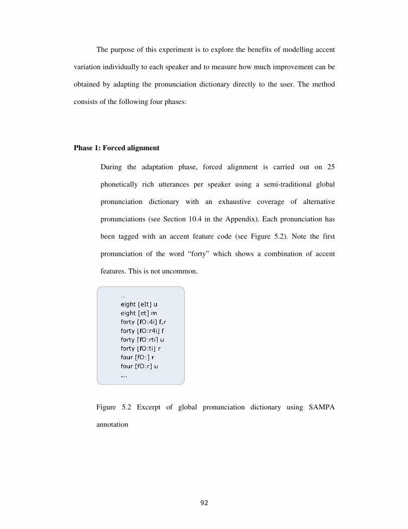
92
The purpose of this experiment is to explore the benefits of modelling accent
variation individually to each speaker and to measure how much improvement can be
obtained by adapting the pronunciation dictionary directly to the user. The method
consists of the following four phases:
Phase 1: Forced alignment
During the adaptation phase, forced alignment is carried out on 25
phonetically rich utterances per speaker using a semi-traditional global
pronunciation dictionary with an exhaustive coverage of alternative
pronunciations (see Section 10.4 in the Appendix). Each pronunciation has
been tagged with an accent feature code (see Figure 5.2). Note the first
pronunciation of the word “forty” which shows a combination of accent
features. This is not uncommon.
Figure 5.2 Excerpt of global pronunciation dictionary using SAMPA
annotation

93
Phase 2: Accent feature identification
An Accent Feature Identification (AFID) tool was created with the purpose
of identifying the accent features of each speaker before the main recognition
begins. AFID is an extension of AID, introduced in Section 4.4.5, and it
analyses the recognition results from the forced alignment showing which
pronunciation variant was chosen for each word. AFID identifies the accent
feature codes for each recognised word and determines the number of
occurrences of each accent feature in the entire adaptation utterances for each
speaker. The accent features with the highest number of occurrences are
marked as the most characteristic individually for each speaker.
In this phase, we are looking for a pattern in the speech. If an accent
feature is judged to be characteristic for the speaker based on the adaptation
utterances, we make the assumption that this feature will also be chosen by
the speaker for other words which have pronunciation variants marked with
the same feature in the dictionary.
Phase 3: Generation of the idiodictionaries
In the third phase, the information about the characteristics of the speakers’
speech obtained in Phase 2 is used to create a model of their phonological
system. These models contain information about which accent features to
activate and which to ignore and they are the key component in the creation
of the idiodictionaries.

94
Phase 4: Recognition
Once the idiodictionaries are created, the system is ready for normal
recognition - this time with the pronunciation dictionary adapted to the
speaker.
The training set and the test set are the same as in the experiments described in
Section 4.4.5 above. In addition to these, an adaptation set was defined for Phase 1 for
dictionary adaptation. The adaptation set contains 25 phonetically rich utterances per
speaker extracted from the ABI corpus. See Section 10.3 in the Appendix.
5.2.2 Findings
For the majority of speakers, a dictionary containing only the non-rhoticity feature
was created in Phase 3 which is to be expected since they are the statistically most
representative variants.
The pronunciation dictionary applied in Phase 2 of both the experiment with
predefined accent dictionaries and the experiment with idiodictionaries contained the
same pronunciation variants. The only difference was how each pronunciation variant
was tagged, i.e. as belonging to a particular accent or to a particular accent feature
respectively.
When all identified features for each speaker are included, accuracy
significantly deteriorates to 30.17% SER which is worse than the baseline. This most
likely happens because features which only occur a few times cannot be considered to
be particularly characteristic of the speaker in question and do thus not provide any
95
reliable information. We therefore defined a threshold for the minimum number of
occurrences needed for an accent feature to make its way into the idiodictionary.
Both the choice of accent features and the number of times they have to occur
in the initial recognition run to be included in the idiodictionary are parameters that
can be tuned towards the data in question. As we saw above, we chose six accent
features and based on the size of the SA set, i.e. 25 utterances, we defined a fixed
inclusion threshold of minimum four occurrences.
A logical expansion of the method for selecting the accent features is to define
the threshold as a percentage of the number of possible occurrences in the SA data
rather than as a fixed threshold. In Section 5.6, we describe an experiment where we
explore this approach. Instead of making a binary decision regarding the accent
features, we give them different probabilities prior to the creation of the
idiodictionary.
The results of the experiments described above are shown in Figure 5.3. As
can be seen in the figure, at 25.82%, the experiments using the predefined accent
dictionaries only led to a relatively modest improvement compared with the baseline
experiment (28.79%). The accent feature experiment, on the other hand, where the
pronunciation dictionary was adapted to create idiodictionaries as described above
saw a significant improvement, at 22.66%, compared with the baseline experiment.
The result from the experiment from Section 4.2.2 where SA was carried out of the
acoustic models has been included here for comparison with the previous best result,
i.e. 24.18%.

96
Recognition performance
0
5
10
15
20
25
30
35
Baseline SA on AM Accent dictionaries Idiodictionaries
SE
R
Figure 5.3 Comparison of idiodictionary experiment with previous
experiments
The idiodictionaries performed 12% better than the accent dictionaries overall
and no speaker experienced a deterioration in performance as a results of the
pronunciation dictionary adaptation. Compared with the baseline, the idiodictionaries
gave an improvement of about 20%. Compared with the previous best result, i.e. SA
of the acoustic models, the idiodictionaries gave a modest improvement of about 6%
relative.
We have presented a new method to deal with the problem of accent variation
in ASR. The primary advantage of this approach is the level of detail with which we
can chose pronunciations for each speaker. The experiments described above show
that a combination of accent feature identification and pronunciation dictionary
adaptation can significantly improve recognition performance. The experiments have
also given new insight into how pronunciation varies. Accent features therefore seem

97
to be a useful alternative to the notion of regional accent when describing accented
speech in detail.
5.3 SA of test dictionary using various numbers of
utterances
In this experiment, we investigate how recognition performance relates to the number
of utterances used in the SA phase for adapting the pronunciation dictionary.
5.3.1 Details of the experiment
The same set-up as in the previous section was employed with the only difference that
the number of adaptation utterances was increased for each test run, thus testing with
5, 10, 15, 20, 25, 40, and 80 utterances per speaker as opposed to 25 utterances in the
previous experiment.
5.3.2 Findings
The results from this experiment are shown in Figure 5.4 below. As one could expect,
we can see that when more data is included in the identification of the most
characteristic accent features of each speaker, the identification becomes more
reliable. The figure also shows that the improvement due to added information seems
to plateau around 25 utterances.

98
Recognition performance
15
20
25
30
35
0 5 10 15 20 25 40 80
Number of SA utterances
SE
R
Figure 5.4 Recognition performance according to number of SA utterances for
pronunciation dictionary adaptation
The first result in the figure (zero SA utterances) reflects the baseline
experiment from Section 4.3.1 above where no adaptation was carried out. It is
interesting to note that with only a few SA utterances (columns 5 and 10), recognition
performance is worse than the baseline. This means that, based on only a few
utterances, the information about the speaker’s accent is not reliable enough to deviate
from the canonical pronunciation dictionary. Only from 15 SA utterances (SER of
26.85%) and above is there enough good data to reliably adapt the pronunciation
dictionary to the user. This may also be because we used the same accent feature
inclusion threshold (as defined in Section 5.2.2) for all the scenarios in this
experiment. At 25 SA utterances, the SER is at 22.66%.

99
5.4 SA of the training dictionary
In Section 4.2, we saw how accent variation can be modelled implicitly within the
acoustic models during training and during SA of the acoustic models. However, we
also saw that the traditional approaches to doing this do not handle accent variation
very well. The problem is that these approaches focus on modelling or shifting the
means of states and they are unable to deal with insertions and deletion in the
phoneme inventory as well as pronunciation variants in the pronunciation dictionary.
In the current chapter, we have seen how the pronunciation dictionary can be adapted
individually to each speaker’s accent.
In the previous experiments in this chapter, we have looked at generating
idiodictionaries for recognition. In this section, we shall attempt to model accent
variation within the pronunciation dictionary used for training the acoustic models.
We hope that this approach will ensure that the correct phone models are updated
during training and that the resulting acoustic models are more robust when exposed
to accent variation.
5.4.1 Details of the experiment
In this experiment, the idiodictionary approach is applied as part of the segmentation
process where the HMM boundaries are defined in the training data.
First, recognition is carried out on the training data using forced alignment.
The set-up is the same as for the previous idiodictionary experiments described above
with the only difference that the adaptation is carried out on the training data and the
training dictionary. This set-up provides us with information about the phonetic

100
characteristics of each training speaker. Once we know which pronunciation is
preferred for each word, we can retrain the acoustic models this time with a better
likelihood that the correct phone models are being updated. This is an iterative
process which gives purer models for each cycle until a plateau is reached. This
plateau is identified by the best recognition result on the test data using various sets of
these enhanced acoustic models.
The training data and the test data are the same as in the previous experiments.
5.4.2 Findings
When carrying out adaptation of the training dictionary, an SER of 16.45% was
obtained. This represents a significant relative improvement of 43% compared with
the baseline. It is even a substantial improvement compared to the previous
idiodictionary experiments. The primary reason for this large improvement is that the
acoustic models are purer. As we saw in Section 4.2.1, the word “cup” may be
pronounced as [k�p] or as [kʊp] depending on who the speaker’s accent. If we do not
deal with this variation at the dictionary level prior to training through some
mechanism like the one proposed here, the acoustic models will be relatively coarse.
However, by generating idiodictionaries for the training speakers, we stand a better
chance of updating the correct phone models during training thereby leading to
improved recognition accuracy.

101
0
5
10
15
20
25
30
35
Baseline SA on test PD only SA on training PD
only
SER
Figure 5.5 Effect of adaptation of the training dictionary
SA of the training dictionary is an iterative complex process, but since the work is
done off-line, it does not add any complexity during recognition.
5.5 SA of the training and the test dictionaries
As we saw in Chapter 4, it is important to be consistent in the methodology which
means that if one feature is available during training, it should also be available
during recognition. In this experiment, we shall therefore carry out SA of the training
dictionary and on the dictionary used for recognition.
5.5.1 Details of the experiment
The training data and test data were the same as in the previous experiments. The
acoustic models used for this experiment were the best performing acoustic models

102
from the previous experiment where SA was carried out on the training dictionary
only. The adaptation set of 25 utterances per speakers was also the same as in the
adaptation experiments above. The set-up was the same as in the other experiments
were idiodictionaries were generated with the only difference that this time, we are
using enhanced acoustic models.
5.5.2 Findings
Combining SA of the training dictionary with SA of the dictionary used for
recognition leads to further improvement as can be seen in Figure 5.6 below.
0
5
10
15
20
25
30
Baseline SA on test PD SA on training
PD
SA on both PDs
SE
R
Figure 5.6 Effect of adaptation of both pronunciation dictionaries
In the baseline experiment, no adaptation was carried out which gave an SER
of 28.79%. The experiment including accent feature based adaptation of the
103
pronunciation dictionary used during recognition gave SER 22.66%. When carrying
out adaptation of the training dictionary only, an SER of 16.45% was obtained. When
carrying out adaptation of both the training dictionary and the recognition dictionary,
an SER of 12.26% was obtained - another significant improvement. As can be seen by
this experiment, the biggest improvement comes from SA of the pronunciation
dictionary used for training. The best result, however, comes from SA of both
pronunciation dictionaries. From these results, we can conclude that the full benefit of
training purer acoustic models materialises when a detailed method of selecting them
is applied during recognition.
5.6 Probability-based selection of accent features
In the experiments above, we have seen significant improvements in recognition
accuracy. The best performance we have seen so far is when idiodictionaries are
created for each speaker both for training and for recognition. In this section, we shall
see if we can improve accuracy further by describing the speaker’s accent with even
more detail.
In the previous experiments in this chapter, the decision about including or
excluding a specific accent feature from the idiodictionary has been binary. Either the
feature was deemed to be characteristic for the speaker in question and the feature
would then be activated throughout the idiodictionary, or the feature failed to meet the
requirements and was then never included in the idiodictionary. However, there were
several cases where the number of occurrences of a feature in the adaptation data was
very close to the acceptance threshold. We hypothesise that improvements can be
gained from considering the features not as rigid rules but rather as statistical

104
expectations and give each of the accent features a probability score for each person
rather than considering them in absolute measures. In the experiment described here,
we will investigate this hypothesis.
5.6.1 Details of the experiment
The purpose of this experiment is to improve recognition accuracy in particular for
borderline speakers, whose result from the adaptation phase showed occurrences of
accent features close to the acceptance threshold. If for example a speaker had five
occurrences of the feature closing and ten occurrences of the feature flapping, then
flapping should be given a higher probability than closing in the idiodictionary. This
provides a more reasonable comparison of the accent features and it allows accent
features, which were below the acceptance threshold, to be included in the
idiodictionary although only with a lower probability score.
The ASR engine used for the experiments above does not have the capability
to include probability weightings for individual pronunciations in the pronunciation
dictionary. For the current experiment, HTK was therefore used instead.
The acoustic models used for this experiment were trained on the WSJCAM0
corpus (Fransen et al. 1994) and the recogniser was prepared in the Department of
Phonetics and Linguistics at University College London. In the previous experiments
in this chapter, we used a complex set of tools, e.g. the Accent Feature Identifier
mentioned above. These tools were created to work with the CREC speech engine
format and it would take a considerable rewrite to convert the tools into HTK format.
Instead, we decided to use the idiodictionaries created using CREC and convert those
into HTK format. We used the information about the accent features identified for

105
each speaker that we gathered in the previous experiments as the source for our
calculation of the probability scores in the idiodictionaries. Due to the amount of
manual intervention needed to carry out this experiment, we only tested the
probability approach on one speaker. We chose speaker uls_m_08 who exhibits
several accent features in his accent. Some of these accent features have a strong
presence, whereas others have a weaker presence in this accent which makes him a
particular good subject for the current experiment. The results are reported as WER.
The idiodictionaries used in the current experiment contain all the
pronunciation variants from the dictionary used in the SA phase and all the
pronunciations have been given individual probability scores. Let us have a look at a
word in the dictionary for illustration. In the original idiodictionary for speaker
uls_m_08, the section covering the word “batter” looks like this:
Figure 5.7 Sample of idiodictionary showing the word “batter” (SAMPA)
In order to include probability scores in the pronunciation dictionary, we first
need to calculate the probability of the occurrence of each accent feature individually.
We use the following equation to get this number:

106
P
aAFp ≡)(
where p(AF) is the probability of a given accent feature, a is the number of actual
occurrences of that accent feature identified in the SA utterances and P is the number
of possible occurrences in those utterances. For speaker uls_m_08, this gave the
following scores:
• non-rhoticity = 0.20 (4 occurrences out of 20 possible)
• closing = 0.48 (10 occurrences out of 21 possible)
• flapping = 0.94 (15 occurrences out of 16 possible)
• anteriorisation = 0.67 (4 occurrences out of 6 possible)
• monophthonging = 0.21 (5 occurrences out of 24 possible)
• h-dropping = 0.06 (1 occurrences out of 16 possible)
Now we know the probability of each accent feature. The next step is to turn
this measure into a probability score for each pronunciation in the dictionary. If there
is only one pronunciation for a given word, it has the label “u” and is given the
probability 1.00. For the word “back”, this looks like this:

107
Figure 5.8 Idiodictionary entry for the word “back” (SAMPA)
If there are two pronunciation variants for the word, the pronunciation variant
that does not have the “u” label is given the probability corresponding to the accent
feature as listed above, e.g. 0.20 for non-rhoticity. The unmarked pronunciation
variant is then given the remaining probability, in this case 0.80. For the word
“Charlie”, this looks like this:
Figure 5.9 Idiodictionary entry for the word “Charlie” (SAMPA)
When more than one accent feature is possible for a given word, the
probabilities are found using the following steps. First, the probability of the
pronunciation variant with a combination of accent features is found using the
following equation:
)()()( 211 AFpAFpvp ⋅=

108
where p(v1) is the probability of the combined-feature pronunciation variant such as
the first variant in Figure 5.10 below displaying the accent features “f” and “r”,
p(AF1) is the probability of the first accent feature and p(AF2) is the probability of the
second accent feature. For the word “batter”, this is 0.94 x 0.20 and the idiodictionary
then looks like this:
Figure 5.10 Sample of idiodictionary showing the word “batter” (SAMPA)
Next the probabilities of the pronunciation variants with just one accent
feature need to be calculated. This is simply done by subtracting the probability of the
individual accent feature from the probability of the pronunciation with a combination
of accent features.
)()()( 112 vpAFpvp =
and
)()()( 123 vpAFpvp =

109
Finally, the probability for the last pronunciation variant labelled “u” is calculated like
this:
))()()((1)( 3214 vpvpvpvp ++=
which can also be written as
))()(()()((1)( 21214 AFpAFpAFpAFpvp ⋅+=
This gives the complete probability scores for the word “batter”:
Figure 5.11 Complete probability scores for the word “batter” (SAMPA)
For this experiment, two recognition runs were carried out. In the first run, the
idiodictionary for speaker uls_m_08 used in the experiments above was used. This
idiodictionary contains no information about probability and only one pronunciation
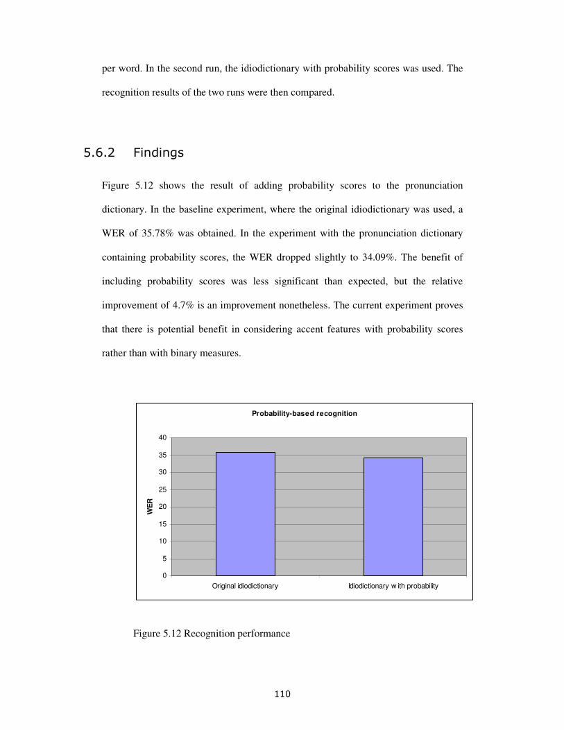
110
per word. In the second run, the idiodictionary with probability scores was used. The
recognition results of the two runs were then compared.
5.6.2 Findings
Figure 5.12 shows the result of adding probability scores to the pronunciation
dictionary. In the baseline experiment, where the original idiodictionary was used, a
WER of 35.78% was obtained. In the experiment with the pronunciation dictionary
containing probability scores, the WER dropped slightly to 34.09%. The benefit of
including probability scores was less significant than expected, but the relative
improvement of 4.7% is an improvement nonetheless. The current experiment proves
that there is potential benefit in considering accent features with probability scores
rather than with binary measures.
Probability-based recognition
0
5
10
15
20
25
30
35
40
Original idiodictionary Idiodictionary w ith probability
WE
R
Figure 5.12 Recognition performance

111
It is to be expected that further improvement could be obtained with the
probability-based method if the acoustic models were trained using the same set-up as
in the experiment in Section 5.4 above, where SA was carried out on the training
dictionary. In addition, the original idiodictionary used in this experiment was
generated with a different ASR engine. Given the same set-up, HTK may or may not
have generated the same idiodictionary.
5.7 Summary and discussion
In the previous chapter, we saw how existing techniques such as SA of the acoustic
models and predefined accent dictionaries fail to model the finer points of accent
variation. In the current chapter, we have presented a novel approach to accent
variation modelling which allows accent variation to be modelled with great detail
and individually to each speaker.
The benefit of describing accent variation in terms of accent features has
clearly been proven in this chapter. Accent features allow us to describe the accent of
a given speaker with a level of detail which has not been available before. By
applying this knowledge, we have been able to adapt the pronunciation dictionary to
fit each user’s specific accent patterns and create idiodictionaries which have
provided us with a substantial improvement in recognition accuracy over any of the
approaches investigated in the previous chapter.
The experiments presented in this chapter have highlighted the complex and
heterogeneous nature of accents in general and we now have hard evidence that the

112
notion of regional accent is an inadequate model for describing accent variation with a
satisfying level of detail in ASR. For this reason and supported by the experiments
above, it makes sense, wherever it is practically possible, to consider the individual
accent variation of each speaker.
Pronunciation dictionary adaptation is a potent tool for dealing with accent
variation, but it cannot achieve the full potential of pronunciation variation modelling
alone. We consider this method to be an extension of traditional SA of the acoustic
models and we expect that a combination of the two will improve recognition
performance even further. In Chapter 7, we shall investigate this hypothesis.
As we saw in Section 5.2, there is significant value in working with a large
phoneme set for accent variation modelling. However, the sufficient amount of speech
data required to model an extended set of phonemes is not always available. For the
purpose of accent variation modelling, it is therefore appropriate to investigate ways
to deal with lack of speech data. In the next chapter, we shall explore this area of
research and see how it applies to accent variation modelling.

6 PHONETIC FUSION
In the current chapter, we shall investigate an approach to deal with lack of speech
data. The approach, termed phonetic fusion, is not accent variation modelling in its
own right, but it is an enabling technique which has the potential to improve the
conditions for modelling accent variation.
6.1 Lack of speech data
Speech data is the enabling factor of the speech recognition process; the one
component that links the algorithms to the real world in which it is applied. This
consequently means that lack of speech data impairs the usability of the speech
engine.
For various reasons, e.g. availability of speakers, cost of recordings or merely
priority, speech data is not always available in the amount one could desire. The
approach to this problem has traditionally been one of accepting the limitations. If no
data were available for a given language, no speech recogniser would be built for that
language. If only a small amount of speech data were available, the phone models
would be very coarse and not very robust when exposed to variation which would
make recognition performance suffer accordingly.
The problem of lacking speech data presents itself in an overall manner, i.e. if
there is little speech data to train acoustic models, the quality of the speech engine
will be poor. The problem is that with small amounts of training data, the means and

114
variants of the acoustic values will be relatively coarse. However, this is also the case
in a more contained manner, namely the lack of training data for specific phonemes.
As we saw in the previous chapter, a good way to ensure a comprehensive
coverage of accent variation is to work with a large phoneme set. It is therefore
important to obtain sufficient training data for each of these phonemes. The problem
is that the presence of some phonemes is often confined to only a few accents and
consequently it may be difficult to find enough training data to build robust phone
models for them.
When collecting speech data for a given language, there will be some
disproportion in the amount of training data available for each phone model simply
because some phonemes are more common than others. The fact that some phonemes
are not present in all accents further emphasizes this imbalance. Some phonemes may
typically only be found in remote areas spoken by relatively few speakers. Ensuring a
substantial amount of occurrences of these phonemes in the speech data collection
therefore often proves to be practically unfeasible. This means that some phonemes
are often underrepresented in speech data collections. An example from British
English is the diphthong /eI/ realised as the phonetic variant [e]. The typical Scottish
pronunciation of a word like “face” is realised with this monophthong, but its
presence is usually limited to a few accent areas.
Whereas lack of speech data in general leads to poor ASR engines, lack of
specific phonemes leads to compromised recognition performance for these phonemes
and thereby for the speakers using them. Such have traditionally been the conditions
for these less common phonemes. This means that speakers with an accent which is
acoustically close to the canonical pronunciation of a language are more likely to

115
obtain good recognition accuracy than speakers with an accent containing some of the
less common phonetic variants. We can then ask ourselves: Is this acceptable? Should
we accept as a fact that some speakers are destined to poor speech recognition
accuracy simply because of their accent? Traditionally, there has not been much
choice. From a practical and financial point of view, it has simply been too
complicated to accommodate all speakers equally.
The work described in this chapter is motivated by the belief that users of
speech recognition engines should have an equal potential of achieving good
recognition performance. In the current chapter, we shall attempt to bring balance to
speech recognition performance across accents by dealing with the problem of lacking
speech data for specific uncommon phonetic variants.
For the reasons stated above, we accept the fact that it can be too difficult to
obtain a sufficient amount of speech data from speakers of accents with exotic
phonemes to reliably train robust phone models for those phonemes. However, we do
not leave it at that. Instead, we go on a hunt for those phonemes elsewhere. We
identify other languages where those phonemes are more common. Having identified
the needed phonemes in other languages brings us to the next problem: How do we
make use of them? The solution proposed in this chapter is called phonetic fusion. It
is described in detail below.
In order to investigate the scope of the challenges related to lack of speech
data and a potential solution, we shall look closer at the following questions in this
chapter:

116
• Can we use speech data from more than one language to train acoustic
models?
• How important is the linguistic affinity between the languages we use?
• Assuming existing speech data from various languages, how little speech data
from a new language is needed to build a speech engine for that language?
• Is it possible to build a set of acoustic models that can support multiple
languages at the same time?
• When incorporating speech data from a different language, is it possible only
to make use of the phonemes missing from the original training data?
These questions will be investigated on the following pages and the theories are put to
the test in experiments.
6.2 Acoustic models trained with small amounts of data
In order to better understand the effect of lacking speech data, the first experiment in
this chapter attempts to simulate the problem. By initially training acoustic models
with a small amount of speech data and gradually increasing the number of training
speakers, we hope to find the relation/balance between amount of speech data and
recognition accuracy.
This experiment also serves as baseline for the experiments which deal with
lack of speech data. The results based on the full training set in this section reflects
the ideal scenario for training acoustic models since only speech data from the target
117
language was included and all the subsequent experiments were expected to give
inferior recognition accuracy.
6.2.1 Details of the experiment
For this experiment, we first trained phone models using five training speakers. We
chose three male speakers and two female speakers following the findings of Adda-
Decker and Lamel (2005) that female speakers tend to perform better than male
speakers in speech recognition tasks. We then went through several iterations of
training phone models, each time doubling the amount of speech data with a 50/50
split between male and female speakers. In total, we completed six different sets of
phone models using 5, 10, 20, 40, 80, 160 speakers and in the final run, we used the
entire training corpus of 67,752 utterances from 205 speakers. The test data consisted
of 2,166 utterances from 16 Italian speakers. Both the training data and the test data
were recordings of command phrases from native Italian speakers collected at Dragon
Systems.
Italian was chosen as test language for these experiments to underline the
cross-linguistic nature of the attempted solution. Italian is moreover generally known
to perform well in speech recognition tasks which reduced the variables in the attempt
to prove the point.

118
6.2.2 Findings
The results are shown as Word Error Rates (WER) in Figure 6.1 below. Not
surprisingly, we see that performance improves as the number for training speakers is
increased.
0.00
1.00
2.00
3.00
4.00
5.00
6.00
7.00
5 10 20 40 80 160 all
Number of ITA speakers
Wo
rd E
rro
r R
ate
ITA
Figure 6.1 WER as a product of number training speakers
The improvement seems to plateau somewhere between 80 and 160 speakers.
When all training speakers are included, the WER is at 1.84%. It can clearly be
observed that lack of speech data leads to significantly inferior recognition accuracy.
6.3 Introducing phonetic fusion
As mentioned above, the work presented in this chapter attempts to deal with the
problem of lacking speech data. The method, termed phonetic fusion, does not remove
119
the need for speech data, but it makes it possible to work around the problem of
lacking speech data for a specific language. The method has successfully been carried
out by other speech researchers. By including speech data from other languages
during training of the acoustic models, it is possible to build a multilingual speech
recogniser (Kumar et al. 2005, Harju et al. 2001, Schultz and Waibel 1998) or a
speech recogniser for a language from which no training data is available (Liu and
Melnar 2005 and 2006, Schultz and Waibel 2001). Parts of the existing research are
referenced in the relevant sections below.
In the current work, the purpose of phonetic fusion is to investigate whether it
can provide the needed phonetic data to model a large phoneme set for better handling
of English accent variation. Our interest in phonetic fusion is therefore merely as an
enabling technology rather than as a goal in its own right.
6.3.1 Uniphone
Since each phone model is trained on speech data from various languages, it is
imperative that the phoneme set is consistent across languages. This is not always the
case with existing computer readable phoneme sets. In English SAMPA, for example,
the character “e” describes the phoneme /ɛ/ whereas in French SAMPA the same
character describes the phoneme /e/. This means that SAMPA is not fit for cross-
language modelling. There are alternative standards, such as X-SAMPA (Wells
(1995)) and Worldbet (Hieronymus (1993)) which have dealt with this problem, but
for commercial reasons it was decided to design a new universal phoneme set termed
Uniphone. Uniphone is universal in the sense that one character represents the same

120
phonetic variant across languages. In Section 10.2 in the Appendix, the British
English phonemes of Uniphone are shown.
The number of distinct phonemes varies considerably from language to
language, but a normal phoneme set for speech recognition usually consists of some
40-60 phonemes per language. Uniphone contains 121 unique phonemes. It is
estimated that there are more than 800 phonemes in the world’s languages (Ladefoged
(2001)), but many of them are fairly exotic and uncommon and we believe that the
coverage of Uniphone is relatively exhaustive in particular for European languages.
The coding of Uniphone was based on SAMPA, but some adjustments were
done to optimise it for ASR usage. The definition of this phoneme set is, as is the case
for IPA and SAMPA, an approximation based on some subjective decisions. There
are cases where there is no clear recommendation as for whether two phonemes from
two different languages should be merged into the same phone model or be trained as
two separate phone models. An example of this is the sibilant /s/ which occurs both
in Italian and Iberian Spanish. In Spain this sibilant is apico-alveolar whereas in
Italian it is lamino-alveolar. There is clearly an acoustic difference in the realisation of
this phoneme /s/ in the two countries, but the question is how different they are. We
can consider them to be two allophones of the same phoneme and use the same
character or we can architect a more refined phoneme set by assigning two distinct
Uniphone characters. The answer is not obvious and cannot be based purely on
acoustic measures and phonetic knowledge. Since the application of Uniphone is
ASR, it is ultimately the ASR engine that decides whether a split or a merge is best. A
split means that there is less training data for each phone model which can make them
less robust. A merge potentially means that the phone model is less pure. A series of

121
experiments was therefore carried out to investigate the cases where the decision
regarding split vs. merge is unclear and the outcome was a more robust universal
phoneme set optimised for speech recognition. In the case of the phoneme /s/, the
results showed that there was a benefit in merging by including speech data from both
Italian and Iberian Spanish in the same phone model.
A somewhat similar approach is carried out in the GlobalPhone project
(Schultz and Waibel (1998)) at Carnegie Mellon University where speech data from
various languages are collected to create multilingual acoustic models. However,
whereas the purpose of the GlobalPhone project is to build a multilingual speech
recogniser, our interest in building a universal phoneme set is a step towards dealing
with lack of speech data and ultimately support a large phoneme set to handle English
accent variation.
6.3.2 How it works
The phonetic fusion approach is quite simple but it is very powerful. Speech data
from several languages are input in the acoustic modelling set-up and during training
the languages are merged into one universal set of phone models. These models can
then be applied during speech recognition of different languages.
Although Uniphone has the potential to cover all phonemes of all languages,
only a relevant subset is active at any given point in time during recognition. This is
controlled by the pronunciation dictionary used for recognition.
122
6.3.3 Benefits and limitations
By traditional methods, it is a costly affair to collect or purchase the amount of speech
data needed to build a recogniser for a new language. Phonetic fusion provides an
alternative which can significantly reduce the budget needed for speech data. The
possibility of building a speech recogniser for a new language without acquiring any
new speech data potentially has a great impact on the speech community. Both the
industry and academia can save a significant amount of money spent on collecting or
purchasing speech data. The industry can respond quickly to customers with a proof-
of-concept system for new languages. Academia can offer recognisers for
traditionally low-priority languages, such as Catalan or Welsh, thus bringing speech
technology to a wider public.
The phonetic fusion method can also be of great value when planning a data
collection. The proof-of-concept system will most likely not perform to product
quality level, but it can highlight recognition problems, e.g. likely digit confusions or
new phonological features not covered in the existing training data. Identifying new
phones gives an important input to designing the data collection which will then have
a strong focus on these phones. If existing training data can be successfully combined
with a data collection, which focuses heavily on missing phones, it may reduce the
needed number of training speakers, thus reducing the cost of data collections.
Phonetic fusion assumes the availability of speech data from several languages
in order to ensure an extensive coverage of phones. The method is also dependent on
a universal phoneme set like e.g. Uniphone described above. These language-
independent phone models can then be applied across languages, e.g. in a multilingual
application. Applying language-independent phone models in a multilingual speech

123
application moreover has the potential to significantly reduce the footprint of the
application because the large universal set of phone models is smaller than having one
set for each language.
In this chapter, we shall look at a few experiments which investigate whether
a) a reasonably well performing Italian speech recogniser can be built without any
Italian speech data and b) how much native Italian speech data is needed to obtain
performance which could be considered product quality.
However, as we shall see below, performance depends on a number of factors.
Some languages obtain better results than others. Nevertheless, it can generally be
assumed that better phoneme coverage means that more languages will obtain
reasonable recognition performance.
6.4 Building a new speech recogniser
This experiment is the first attempt at applying speech data from various languages
during training of the acoustic models. This work was first presented in Tjalve (2005).
In this experiment, we test the applicability of phonetic fusion by trying to build an
Italian speech recogniser without Italian speech data. Schultz and Waibel (2001) call
this method cross-language transfer. This experiment thus tries to evaluate the
language-independent nature of the acoustic models trained with the phonetic fusion
method.
It is not realistic to expect the same level of recognition accuracy as with a
traditional speech engine using a set of language dependent acoustic models, but we
hope that the accuracy corresponds to a decent proof-of-concept recogniser.

124
6.4.1 Illustration of methodology
Figure 6.2 illustrates how the phone models needed to recognise an Italian word can
be trained on speech data from English, Spanish, German and French. We can for
example see that based on the four words in the figure, the phone model for [a] is
trained on data from Spanish and French, whereas the phone model for [ʦ] only gets
training data from German.
Figure 6.2 Illustration of phonetic fusion
This figure illustrates the method for training monophones. However, since we
are training PICs, the first [a] in “arriba” would not be part of the same phone model
as the second [a]. The method is slightly more complex and the figure is therefore for
illustration purposes only. If we imagine that our training data only consists of the
125
four words “again”, “arriba”, “Zeit”, and “hôpital”, we can create a pronunciation
dictionary containing the correct phones for the Italian word “ragazzo”. The phoneme
[r] would come from Spanish, [a] from Spanish and French, [g] from English, [ʦ]
from German, and [o] from French. Note that the [a] data comes from more than one
language. This is a very common situation which underlines the universal nature of
the method.
The training data used for the experiments reported below do of course contain
many more words than the four mentioned above and can thus cover a large number
of Italian words.
6.4.2 Missing phonemes and acoustic proximity
An issue, which needs attention when training PICs exclusively on data from
languages other than the target language, is the fact that the training data may not
include all the phonemes needed for the test data. We approach this problem by
identifying the closest phonetic match and adjusting the pronunciation dictionary
accordingly. The identification of the closest phonetic match can be carried out with a
knowledge-based approach or a data-driven approach. In Liu and Melnar (2005,
2006), a data-driven approach to this problem is described. They calculate the
phonetic similarity between the candidate phoneme and the target phoneme based on
a comparison of acoustic models trained on the source languages and acoustic models
trained on the target language. The benefit of this approach is that the identification of
the closest phonetic match is based on actual data from the source languages and the
target language. However, the drawback is that it requires speech data from the target
126
language which was the problem we initially wanted to address. Kumar et al. (2005)
describe an approach to build a multilingual speech recognition system. They
combine training data from two similar languages, Tamil and Hindi, and one
dissimilar language, American English. They use the Bhattacharyya distance, a
statistical model for measuring the similarity between two probability distributions, to
measure the phonetic distance between phones from different languages to decide
whether they should be combined into one phone model are whether they should be
trained as two separate phone models. They find that the loss of accuracy due to the
inclusion of training data from multiple languages is reduced by using the
Bhattacharyya distance approach.
In the current work, we chose the knowledge-based approach to identifying
the closest phonetic match, because we wanted to investigate the potential of the
method without the availability of any speech data from the target language at all. The
identification of the closest phonetic match was initially based on the number of
differences in distinct features between the candidate phoneme and the target
phoneme. However, it quickly became clear that not all distinct features are equally
important for distinguishing phones in ASR. The measures were therefore combined
with a subjective weighting. The difference between /t/ and /θ/ for example is easier
for the speech recogniser to identify than the difference between /t/ and /tʰ/. The
distinct feature [±continuous] was consequently given more weight in the calculation
of the phonetic distance than the feature [±aspirated].

127
Since we were training PICs, the definition of the closest match for missing
phones had to be considered not only for the target phone but also for the left and
right context phones.
Basing the choice of phonemes on the closest match is of course a
compromise compared to having the exact phoneme available and it is to be expected
that the more occurrences there are of missing phonemes and the larger the distance is
between the missing phoneme and the closest match, the more recognition
performance will suffer.
6.4.3 Details of the experiment
In this experiment, training data from English, Spanish, German and French was
included to train PICs. A total of 235,831 command and control utterances from 878
speakers across the four languages were used to train the acoustic models. These
multilingual acoustic models were validated on the same test set as in Section 6.2
above, i.e. 2,166 utterances from 16 Italian speakers. During recognition, only a
relevant subset of these acoustic models, corresponding to the Italian test set, was
used.
6.4.4 Findings
As shown in Figure 6.3, with a WER of 4.68% the recognition accuracy for this
experiment was significantly inferior to the condition where only Italian speech was
used during training of the acoustic models.

128
0.00
1.00
2.00
3.00
4.00
5.00
ITA only All languages minus ITA
Wo
rd E
rro
r R
ate
Figure 6.3 Performance comparison between conventional acoustic models
and acoustic models trained using the phonetic fusion approach
Although performance decreased compared with the traditional monolingual
set-up, recognition accuracy was still good. This experiment has proven that phonetic
fusion makes it possible to build a proof-of-concept speech recognizer for a language
for which no data is available.
In this experiment, languages from two language families were included. The
next step is to see whether there is any benefit in dividing the training data according
the language family relation.
6.5 Phonetic fusion by language family
This section investigates the importance of the linguistic affinity between the
languages used during training of the acoustic models and the language used for
testing. The training data was divided into two sets: one for data from Germanic

129
languages (English and German) and one for data from Romance languages (Spanish
and French).
There were cases where the training data was missing specific phonemes
needed for the test data. As in the previous experiment, we dealt with this problem by
replacing them with other phonemes based on the acoustic proximity approach
described above to minimise the negative impact of these missing phonemes.
6.5.1 Germanic training data
For this experiment, context-dependent acoustic models were trained exclusively on
speech data from Germanic languages. A total of 138,789 utterances from 508
German and English speakers were used for training. The acoustic models were
validated on the same Italian test set as above, i.e. 2,166 utterances from 16 Italian
speakers.
Compared to the previous experiment where data from both Germanic and
Romance languages was included in the training data, this experiment exhibited a
significant deterioration in accuracy which suggests that the language family relation
between the training data and the test data is a significant factor.
Figure 6.4 Accuracy of Germanic acoustic models

130
It is worth mentioning that the number of missing phonemes from the training data
needed to match the test data was high compared to the previous experiment. It
therefore seems reasonable to conclude, as posited above, that a high number of
dependencies on acoustic proximity leads to poor acoustic models.
6.5.2 Romance training data
The acoustic models used in this experiment were trained exclusively with speech
data from Romance languages. A total of 97,042 utterances from 370 speakers of
Spanish and French were used for training. The acoustic models were validated on the
same test set as above. The training data and the test data is consequently from the
same language family.
Figure 6.5 Accuracy of Romance acoustic models
6.5.3 Findings
The experiments above show the effect of separating the training data according to
language family. In a similar experiment, Schultz and Waibel (2001) conclude that
prior knowledge about the source language is indeed important when using
monolingual acoustic models for cross-language transfer. However, for cross-
language transfer based on acoustic models trained on multiple languages, they
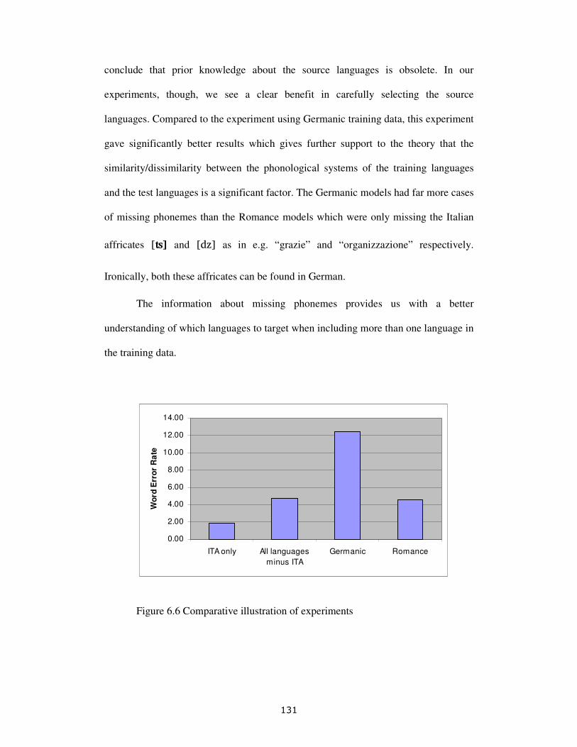
131
conclude that prior knowledge about the source languages is obsolete. In our
experiments, though, we see a clear benefit in carefully selecting the source
languages. Compared to the experiment using Germanic training data, this experiment
gave significantly better results which gives further support to the theory that the
similarity/dissimilarity between the phonological systems of the training languages
and the test languages is a significant factor. The Germanic models had far more cases
of missing phonemes than the Romance models which were only missing the Italian
affricates [ʦ] and [dz] as in e.g. “grazie” and “organizzazione” respectively.
Ironically, both these affricates can be found in German.
The information about missing phonemes provides us with a better
understanding of which languages to target when including more than one language in
the training data.
0.00
2.00
4.00
6.00
8.00
10.00
12.00
14.00
ITA only All languages
minus ITA
Germanic Romance
Wo
rd E
rro
r R
ate
Figure 6.6 Comparative illustration of experiments

132
Figure 6.6 shows a comparison of the results so far in this chapter. It is
interesting to note that the acoustic models trained only on Romance data performed
better than the acoustic models trained on all the languages minus Italian. So,
although the occurrences of missing phonemes were kept to a minimum by the
Romance training data, the results seem to indicate that the presence of the German
and English data contaminated the acoustic models when used in an Italian
application. In other words, some of the phonemes which German and/or English
share with Italian were not fully compatible with the Italian test data. A detailed
analysis of the error patterns confirms this conclusion. Words with an initial unvoiced
plosive, e.g. ‘telefono’, tend to be more easily recognised when no German/English
data is included in the training set. The German and English pronunciation of these
phonemes typically includes an aspiration which is not seen in the Italian
pronunciation. One could then argue that there is good evidence for splitting up e.g.
/t/ into /t/ and /tʰ/, but since we are not interested in using the phoneme /tʰ/, it was
more appropriate to split up the training data instead.
Although a proof-of-concept recognizer may be of considerable interest, the
quality of such a recognizer is still not good enough for most applications. The next
step is to try to improve performance by adding training speakers of the target
language.
6.6 Gradual addition of Italian speakers
In the previous experiment, we saw how it is possible to successfully build a proof-of-
concept speech recogniser without speech data from the target language. However,

133
the quality of such a proof-of-concept recogniser is not good enough for most
applications. In the current experiment, we investigate how much training data from
the target language is needed to improve the recogniser from proof-on-concept level
to product-level recognition performance.
6.6.1 Details of the experiment
We use the same set-up as in the previous experiment, i.e. training data of 97,042
utterances from 370 speakers of Spanish and French. In addition to this, we gradually
added Italian training data. We started with five Italian speakers and doubled the
number for each new training session until all 205 Italian training speakers were
included. Each set of acoustic models were validated on the same test set as above.
6.6.2 Findings
Figure 6.7 shows the effect of gradually adding speech data from the target language
to the training data. The baseline (number of Italian speakers = 0) is the result from
the previous experiment where Romance (Spanish and French) training data was used.
The performance quickly improves as the first few speakers are added, but the
improvement seems to plateau at around 40 speakers with a WER of 1.57%.

134
0.0
1.0
2.0
3.0
4.0
5.0
0 5 10 20 40 80 160 all
Number of ITA speakers
Wo
rd E
rro
r R
ate
Figure 6.7 Effect of adding Italian speakers to training data
In Figure 6.8 below, the results from the experiment in Section 6.2 about small
amounts of training data are shown next to the results from this experiment to better
compare the two sets of experiments. Since the acoustic models cannot be built
without any speech data at all, there is no result for Italian only at 0 speakers. We can
see that it is possible to significantly reduce the number of training speakers needed to
obtain product-level recognition accuracy.

135
0
1
2
3
4
5
6
7
0 5 10 20 40 80 160 all
Number of ITA speakers
Wo
rd E
rro
r R
ate
ITA only
Fusion
Figure 6.8 Effect of adding Italian speakers to training data
An interesting observation can be made by looking at the lowest WER for
both sets of experiments. The best score using the phonetic fusion method
outperforms the traditional approach. This could indicate that the Italian training set is
lacking data for some phones. The addition of data for those phonemes from other
languages may then have made those phone models more robust which could improve
recognition accuracy. A detailed analysis of the error patterns confirms this
conclusion. Words with the palatal lateral approximant /ʎ/, e.g. “biglietto”, tend to
get better recognition when Spanish speech data is included in the training set.
This is exactly the behaviour we were hoping to find. In the beginning of this
chapter, we saw how obtaining sufficient training data for the more uncommon
phonemes, such as [e] in the typical Scottish accent, is often problematic. The finding
from the lowest WER for the two approaches suggests that phonetic fusion can

136
improve recognition performance for specific phonemes. In the last experiment of the
current chapter, we will investigate the potential of this finding and attempt to come
up with a more intelligent way of handling specific phonemes.
6.7 Multilingual speech recognition
In the previous experiments in this chapter, we have witnessed the ability of phonetic
fusion to enable cross-language acoustic modelling. In this section, we shall look at
cross-language recognition.
The motivation for this experiment is to explore the potential and the
limitations of the phonetic fusion method and to investigate to what extent the idea of
modelling and recognising speech from multiple accents can be extended to
modelling and recognising speech from multiple languages.
6.7.1 Details of the experiment
For this experiment, two scenarios for each language were tested: one monolingual
and one multilingual. The monolingual scenario represents the traditional speech
recognition situation, where training data from one language has been used to create
acoustic models which in turn have been used for recognition of speech data from that
same language. In the multilingual scenario, three languages were included during
training of the acoustic models and recognition was carried out with a recognition
grammar which contained a valid path for each language thus allowing all three
languages to be active at the same time. This way, both the utterance and the language
were recognised in one pass. By comparing the performance of the two scenarios for

137
each language, we can evaluate the ability of phonetic fusion to carry out cross-
linguistic recognition.
Details of the speech data used for this experiment are shown in Figure 6.9
below.
Figure 6.9 Details of speech data
6.7.2 Findings
The results of these experiments are presented in Figure 6.10 below as Word Error
Rate. As one would expect, the multilingual scenarios performed worse than the
traditional monolingual scenarios.
Figure 6.10 Comparison of monolingual and multilingual scenarios

138
The most likely reason for this is the complexity of the recognition grammar.
Significantly more valid grammar paths are supported in the multilingual scenario
leading to increased confusion. A detailed analysis of the results supports this
conclusion, i.e. the additional errors in the multilingual scenario tend to be recognition
results where the recogniser went down the wrong language path. Schultz and Waibel
(1998) observe a slightly greater degradation in a similar experiment with five
languages.
As an extension to the current experiment, the method was applied in a more
extreme application to explore its limits. Speech data from English, French, Spanish,
Italian and German were used to train multilingual acoustic models. A grammar
supporting digit recognition was created for languages as different as Danish,
Hebrew, Tamil, Irish, Dutch, Japanese and Arabic. For Hebrew, Dutch, Japanese and
Arabic, recognition accuracy was relatively high (85-95%) whereas for Danish, Tamil
and Irish the accuracy was quite low (below 60%). Although the range of recognition
accuracy across languages was considerable, it was possible to use these acoustic
models for digit recognition in very dissimilar languages and as a proof of concept the
method worked.
6.8 Non-native speech recognition
Up until this point, our experiments have focused on accented speech related to native
speakers only. However, non-native accented speech is also known to cause problems
for ASR engines. In Section 4.4.1, we looked at existing approaches to identifying the

139
accent of a non-native speaker. In this section, we shall investigate ways to improve
speech recognition for non-native accented speakers.
Bouselmi et al. (2005) describe an approach to dealing with non-native speech
where forced alignment is carried out with a set of acoustic models for the native
language (L1) as well as with a set of acoustic models for the spoken language (L2) to
identify phones that are confused. The same language was tested during recognition
for both sets of acoustic models. Instead of merging the training data and building
combined acoustic models, they use the information from this alignment to modify
the existing HMMs by defining new state transitions between phones to accommodate
the non-native pronunciations. Using this approach, they obtain a significant
improvement over their baseline where no information about L1 was taken into
consideration. In Stemmer et al. (2001), an approach to dealing with foreign words in
German is presented. They use training data of English words pronounced by German
speakers. The problem with this approach is that this type of data is very difficult to
obtain. Kessens (2006) evaluates adaptation techniques to deal with non-native speech
recognition and obtains good improvements.
In this section, we shall investigate to what extent phonetic fusion can improve
recognition of non-native speech. The problem is of course closely linked to the
language proficiency of the speaker, but some likely problem areas can be identified
nevertheless. We can divide the phonological challenges into two groups: a)
phonological similarities and b) phonological differences between the speaker’s
mother tongue (L1) and the target foreign language (L2). The phonological
differences between L1 and L2 are likely to be the greatest contributor to ASR
problems. However, in the experiment described in this section, we choose to focus
on the phonemes that are shared between the two languages, exemplified by German

140
and French, merely for the sake of proving the point that phonetic fusion can also
improve recognition of non-native speech. More investigation can be done here, but it
falls outside the scope of the current work to go deeper into the challenges
surrounding non-native speech recognition.
6.8.1 Details of the experiment
In this experiment, a traditional speech recogniser was compared with a recogniser
based on phonetic fusion. Both were tested on non-native speech data. In the
traditional scenario, the acoustic models were trained on 54,852 utterances from 190
French speakers. In the phonetic fusion scenario, 75,123 utterances from 270 German
speakers were added to the French training data by phonetic fusion as described in
detail in Section 6.4. Parts of the phoneme inventories of the two languages overlap.
The phone models trained for those phonemes were updated by speech data from both
languages. The resulting bilingual acoustic models were used during recognition. A
traditional monolingual French grammar was created for testing and the pronunciation
dictionary contained standard French pronunciations and did thus not explicitly
attempt to deal with the non-native accent variation. The test data consisted of 56
recordings of 8 German speakers speaking in French at varying levels of proficiency.
The test data was extracted from the BonnTempo-Corpus (Dellwo et al. 2004) and
consisted of read phrases from a story. With 92 supported words, the vocabulary was
very small.

141
6.8.2 Findings
Applying phonetic fusion to non-native speech recognition gave a significant
improvement when over the traditional approach as shown in Figure 6.11.
With the traditional approach where the acoustic models were trained on
French speech data only, a WER of 5.36% was obtained. When training acoustic
models on both German and French speech data, the WER decreased to 3.58% which
represents a relative improvement of 33%.
Non-native speech recognition
0
1
2
3
4
5
6
Traditional Phonetic Fusion
Wo
rd E
rro
r R
ate
Figure 6.11 Two approaches to non-native speech recognition
The effect of adding data from the speaker’s mother tongue depends on how
strong a foreign accent the speaker has. Although the test set is very small, the results
seem to show a clear benefit in adding data from the speaker’s L1 to the training data,
when recognition is carried out on L2.
142
6.9 Targeted phone modelling
In the previous chapter about accent features, we hypothesised that the inclusion of
speech data from other languages would make it possible to support a large phoneme
set for detailed accent modelling when training data for some of the more exotic
phonemes was lacking. In the experiments presented in the current chapter, we have
indeed proven that phonetic fusion makes it possible to include new phonemes in the
acoustic models.
However, the phonetic fusion experiments also showed that some speech data
helps whereas other speech data deteriorates performance. Even keeping the
additional speech data to linguistically neighbouring languages does not necessarily
ensure success. Ideally, only the phonemes that are missing from the target language
should be modelled but up until this point of the current work, as well as traditionally
in the speech industry, the inclusion of speech data for training of the acoustic models
has been a decision between all and nothing. This has also been the case in the
existing research in cross-language acoustic modelling (Liu and Melnar (2005, 2006),
Kumar et al. (2005), Harju et al. (2001), Schultz and Waibel (1998, 2001)). However,
this need not be the case. In the experiment described in this section, we present a
novel method for dealing with the lack of speech data by targeting specific phones
rather than entire corpora. We term this method targeted phone modelling. This way,
we ensure that only the missing phone models are added to the training set and we
thereby avoid contamination of the existing good data sets.

143
6.9.1 Details of the experiment
For the experiments reported here, the semi-closed vowels [e] and [o] were taken
from German training data to deal with monophthonging in British English. The
experiments described in this section focused on improving recognition accuracy for
British English speakers with a high score for the accent feature monophthonging.
The training data consisted of a total of 145,738 utterances from 528 English
and German speakers. However, of all the German training data, context-dependent
phone models were only trained for the two phonemes mentioned above. The test data
consisted of 973 utterances from 7 English speakers each with a strong presence of
the accent feature monophthonging. The pronunciation dictionary used in this
experiment was the adapted dictionary with the accent feature monophthonging
active.
During training, we include speech data from the target language along with
speech data from another language where the phoneme is more common. However,
rather than including all the data from the other language as training data, we only
target the relevant phones. All the other phones are converted into Ignore Phones,
represented by the symbol /IGN/. This conversion is done after segmentation of the
acoustic signal to avoid that the alignment with the training data is compromised. The
phone model for /IGN/ is thus trained on greatly diverse acoustic data making it of no
use for recognition. The severely coarse /IGN/ phone model is therefore disregarded
in the clustering process simply by not asking any linguistic questions about them.
Since we are building context-dependent phone models, the target phone and
the two surrounding phones are kept unchanged, whereas the rest are changed to

144
Ignore Phones. See the phonetic transcription of the verb “wiederholen” below for
illustration:
“wiederholen” /v i: d 6 h o: l @ n/ � /IGN IGN IGN IGN h o: l IGN IGN/
Figure 6.12 illustrates how we use the phone model trained on words like
“wiederholen” to support specific phonemes for English pronunciation variants as in
e.g. the word “whole”. The variant exhibits the feature monophthonging.
Figure 6.12 Illustration of phonetic fusion
Figure 6.12 also highlights how the majority of the German training data is
discarded leaving us only with the data we need.

145
6.9.2 Findings
In this experiment, we chose to focus on speakers with a strong presence of the accent
feature monophthonging. In the baseline experiment, these seven speakers obtained an
average SER of 34.29%. When applying targeted phone modelling, these speakers
saw a significant relative improvement of 18% giving them an average of 28.12% as
illustrated in Figure 6.13.
Effect of Targeted Phone Modelling
0
5
10
15
20
25
30
35
40
Traditional Targeted Phone Modelling
Wo
rd E
rro
r R
ate
Figure 6.13 Effect of targeted phone modelling
It is expected that some further improvement can be obtained by combining
targeted phone modelling with the idiodictionary approach. In the next chapter, we
shall investigate the impact of combining these two approaches.

146
6.10 Summary and discussion
In the previous chapter about accent features, we discussed how a large phoneme set
improves the conditions for accent variation modelling. However, it takes a
considerable amount of speech data to support a large phoneme set and it often proves
difficult to find enough suitable speech data to support the additional phonemes.
In the beginning of the current chapter, we saw how lack of training data has a
negative impact on the robustness of the acoustic models. We also saw that it is
possible to include speech data from other languages to make the acoustic models
more robust. This can be done either in an absolute manner or by including specific
phonemes only. This technique has several potential benefits. It can reduce the budget
spent on speech data. It makes it possible to build a proof-of-concept ASR system for
a new language or even create a multilingual application. It can improve recognition
performance for non-native speakers. Including speech data from more than one
language also allows us to increase the size of the phoneme set for a specific target
language and thereby model accent variation more reliably.
In the next chapter, we shall attempt to combine the various techniques
introduced and explored in the current work for improved accent variation modelling.

7 PUTTING IT ALL TOGETHER
7.1 Evaluation of previous experiments
In the previous chapters, we have investigated many different approaches to accent
variation modelling. We have studied the existing research in this area and reproduced
the most pertinent experiments to establish benchmarks for how the current state of
the art performs on the test data used in the current work.
A few novel approaches to accent variation modelling have been developed
and described on the pages above. They have proven their worth as stand-alone
techniques, but in this chapter we shall explore the benefit of combining some of the
most potent methods presented so far. Our baseline was an ASR engine using a
traditional approach to training the acoustic models and a canonical pronunciation
dictionary. No adaptation was carried out. This set-up gave an SER of 28.79%. Our
best result so far was obtained with idiodictionaries, i.e. by performing SA of the
pronunciation dictionary used for training the acoustic models and on the
pronunciation dictionary used for recognition. With this set-up, we achieved an SER
of 12.26%. On the pages below, we shall see whether we can further improve this
result.
7.2 Idiodictionaries and SA of the acoustic models
In the previous two chapters, we have seen the benefits of SA of the acoustic models
and of SA of the pronunciation dictionaries, i.e. creation of idiodictionaries. In

148
Chapter 5, we hypothesised that SA of the pronunciation dictionaries could work in
conjunction with traditional techniques for SA of the acoustic models. In the current
section, we shall put this hypothesis to the test.
7.2.1 Details of the experiment
The speech data is the same as in previous experiments, i.e. training data of 70,615
utterances from 258 British English speakers and test data of 22,795 commands and
short sentences from 158 speakers of various British accents. The adaptation set is the
same as in the other adaptation experiments above. We use the same enhanced
acoustic models as in Section 5.4 which means that SA of the pronunciation
dictionary used for training is already included in this experiment.
In the adaptation phase, two processes are initiated: SA of the acoustic models
and SA of the recognition dictionary. These two processes work independently of
each other and they generate two separate outputs: a set of adapted acoustic models
and an idiodictionary for each speaker.
Based on the adapted set of acoustic models and the idiodictionary for each
speaker, recognition is carried out on the full test set.
7.2.2 Findings
In the baseline experiment, where no adaptation was carried out, we obtained an SER
of 28.79%. In the MLLR experiment, where SA was carried out on the acoustic
models only, an SER of 24.18% was obtained. Performing SA of the training and the
test dictionaries gave an SER of 12.26%. When combining SA of the acoustic models

149
and SA of both pronunciation dictionaries, an SER of 11.04% is obtained. This
represents a significant relative improvement of 62% compared with the baseline.
0
5
10
15
20
25
30
35
Baseline SA on AM SA on both PDs SA on AM and
both PDs
SE
R
Figure 7.1 Recognition performance with various scenarios
The results show that the biggest individual improvement comes from SA of
the pronunciation dictionaries and that a combination of SA of the acoustic models
and the pronunciation dictionaries provides the best accuracy.
In Chapter 4, we saw that the strength of SA of the acoustic models is
primarily in the handling of pronunciation variation due to physiological differences.
In Chapter 5, we saw that SA of the pronunciation dictionaries is very capable of
handling accent variation. The experiment described here confirms that SA of the
pronunciation dictionary can indeed be successfully implemented as an extension of
traditional SA of the acoustic models rather than as a stand-alone method and these
two adaptation techniques can complement each other.

150
7.3 Idiodictionaries and targeted phone modelling
In the first idiodictionary experiment1, we discussed the benefit of working with a
large phoneme set. We also discussed the limitations related to this approach when
working with a traditional monolingual speech corpus. However, in the previous
chapter we found a way to work around this problem. Phonetic fusion and targeted
phone modelling provide a method of including speech data from more than one
language which makes it possible to increase the size of the phoneme set and thereby
model accent variation with greater detail.
In this section, we shall investigate the effect of combining SA of the
pronunciation dictionaries with targeted phone modelling. Targeted phone modelling
is thought to be a better candidate for the current purpose than phonetic fusion since it
is optimised for the target language which in this case is English.
7.3.1 Details of the experiment
As in the experiment described in Section 6.9, the acoustic models used in this
experiment were trained on both English and German speech data. The training data
consisted of a total of 145,738 utterances from 528 English and German speakers.
Targeted phone modelling, as described in the previous chapter, was carried out to
allow support for the two semi-closed vowels [e] and [o] which were needed to deal
1 See Section 5.2

151
with monophthonging in some British English accents. The size of the phoneme set
thus increased to 50 phonemes. See this phoneme set in Section 10.2 in the Appendix.
The training process was further optimised by the inclusion of training
idiodictionaries following the process described in Section 5.4. This step was not
carried out for the German training dictionary. Idiodictionaries were also created
during the adaptation phase prior to recognition. The test data and the adaptation set
are the same as in the other adaptation experiments described above.
7.3.2 Findings
Figure 7.2 shows how SA of the pronunciation dictionaries (idiodictionaries) and
targeted phone modelling perform individually and combined.
Recognition performance
0
5
10
15
20
25
30
Baseline Targeted
Phone
Modelling
Idiodictionaries Idiodictionaries
and Targeted
Phone
Modelling
SE
R
Figure 7.2 Recognition performance with various scenarios

152
We can see that the greatest improvement come from the idiodictionaries. The best
result is achieved by combining idiodictionaries with targeted phone modelling. This
gives an SER of 12.11% which is slightly better than idiodictionaries alone at 12.26%.
Compared with the baseline, this represents a significant relative improvement of
60%.
A closer study of the results reveals roughly the same recognition pattern as in
the initial experiment with targeted phone modelling, i.e. a few speakers with a strong
presence of the accent feature monophthonging experienced a significant
improvement, whereas most other speakers saw little or no change compared to the
experiment with idiodictionaries only.
7.4 Everything combined
In this final experiment, we shall attempt to combine the most significant approaches
described in the above chapters into one synergetic set-up. These approaches are:
• Accent feature/idiodictionary approach on training and test dictionary
• Large phoneme set provided by targeted phone modelling
• SA of the acoustic models
The approach described in Section 5.6 where probability scores were added to the
idiodictionary would have made a good addition to this experiment, but the option to
include probability scores in the pronunciation dictionary is not available in CREC
and the Uniphone-based approach has not been created for HTK.

153
The first two of the three approaches in the current experiment are new
techniques developed as part of the research presented here. The last approach is a
well-established technique and it has been included here to present the best usage of
available techniques for handling pronunciation variation in ASR.
7.4.1 Details of the experiment
The training data, the adaptation data and the test data are the same as in the previous
experiments described in this chapter. In this experiment, we used the acoustic models
trained as part of the experiment described in the previous section. They were trained
on English and German speech data and SA was carried out on the training dictionary
to generate idiodictionaries. SA was also carried out on the acoustic models and on
the recognition dictionary and recognition was subsequently carried out using the
adapted acoustic models and the idiodictionaries.
7.4.2 Findings
Figure 7.3 shows the results of the baseline experiment, the initial experiment of each
approach included in this section and finally the results of the combined experiment
where all approaches were included.

154
Recognition performance
0
5
10
15
20
25
30
35
Baseline Targeted Phone
Modelling
SA on AM Idiodictionaries Idiodictionaries,
SA on AM and
Targeted Phone
Modelling
SE
R
Figure 7.3 Performance with various scenarios
We can see that application of the individual techniques improves recognition
accuracy. However, when combining all three techniques, the SER is reduced to
10.39% which represents a relative improvement of 64% over the baseline and it is
the best result of all the tested scenarios in the current work.
7.5 Summary and discussion
In the previous chapters, we have seen how various approaches to modelling accent
variation can improve recognition accuracy on accented speech. We obtained the best
individual improvement by adapting the training dictionary to the individual training
speaker, but many of the other approaches investigated in the current work also gave
significant improvements.

155
It is interesting to note that both SA of the acoustic models and SA of the
pronunciation dictionary improve performance independently of each other on the
same test set. This proves that both approaches should be considered when
recognition performance is an issue. The question is then how do you know which
method to carry out? In this chapter, we have successfully combined both approaches
which gave us the best recognition result of all our experiments. We have thus proven
that it is possible to establish a balance between these two approaches and that they
can coexist in a speech application. This has provided us with a new recommended
scenario to deal with pronunciation variation in general and accent variation in
particular.

8 DISCUSSION AND CONCLUSION
8.1 Summary and discussion
In this thesis, we have taken a close look at what accent variation is and why it is a
challenge to ASR engines. Motivated by the belief that the imbalance in recognition
accuracy between speakers of different accents is unacceptable, we have investigated
the existing research within accent variation modelling in speech recognition. We
have reproduced some of the most typical approaches to obtain a benchmark for the
performance of the state of the art today. We have concluded that the most typical
approaches to dealing with accent variation are not flexible enough to model the
details of accent variation:
• Merely adding alternative pronunciations to the pronunciation dictionary is
likely to increase confusion between entries.
• SA of the acoustic models is unable to deal with changes in the phoneme
inventory and pronunciation variants in the pronunciation dictionary.
• Selecting the most appropriate pronunciation dictionary from a number of
predefined accent dictionaries in inadequate because accent types are more
numerous and more variable than what can be captured in a few dictionaries.
The alternative presented in this thesis is to consider accent variation as
something which is characteristic to each speaker individually. In order to model
accent variation individually to each speaker, we work with accent features instead of

157
predefined accent groups and we adapt the pronunciation dictionary accordingly to
create an idiodictionary for each speaker. This approach gives significant
improvements compared with the typical approaches to accent variation modelling.
There is clearly potential value in working with a large phoneme set when
modelling accent variation with great detail. Since speech data is often lacking for
specific phonemes, we have chosen to include training data from other languages
where those phonemes are more common in order to improve the robustness of the
acoustic models. We have managed to this by including entire speech corpora and by
targeting specific phonemes individually. This phonetic fusion of languages has
further improved recognition accuracy of the accented speakers in our experiments.
The methods presented in this thesis have been proven to be capable of
significantly improving recognition accuracy of accented speakers, but we
acknowledge that the methods can work in combination with existing techniques such
as SA of the acoustic models for further improvements.
8.2 Thesis contributions
The primary accomplishment of the research presented here is the capability of
automatically modelling accent variation individually for each speaker. The creation
of idiodictionaries and the application of these during recognition provide a level of
detail in accent variation modelling which can be of great benefit for accented
speakers. Speech applications which automatically adapt to the user for improved
recognition accuracy and enhanced user experience have the potential to help
facilitate a wider adoption of speech technology.

158
By highlighting the complex and heterogeneous nature of accents and the
advantage of considering speakers as individuals in the context of accent variation
rather than as members of a group, this method may also influence how accent
variation is defined and treated in accent research outside of speech technology. An
interesting sociolinguistic aspect of this is potential new insight into how groups form
and change. Accent features could prove to be instrumental in this analysis.
The possibility of including speech data from several languages during
training of the acoustic models has several advantages. It makes it possible to build a
proof-of-concept speech recogniser for language for which no speech data is
available. It can improve recognition performance for non-native speakers by
focusing on the characteristics of their mother tongue. It enables the possibility of
working with a large phoneme set which is important for accent variation modelling.
By recycling speech data across languages, phonetic fusion also makes it possible to
save significant funds spent on collecting or acquiring speech corpora. The idea of
phonetic fusion is not new as such, but the capability of only including the relevant
parts of speech corpora by targeting specific phone models is new and has the
potential to provide purer and more robust acoustic models.
Our discussion about the distinction between phonetic and phonological
information has highlighted some of the characteristic differences between these two
levels of description within ASR. The benefit of making an effort out of this
distinction has paid off in a few of our experiments and we have managed to extract
phonological information from phonetic data.
There are certain aspects of the experimental set-up which it has not been
possible to publish due to the commercially sensitive agreement under which the

159
current research was made. This is primarily CREC, the ASR engine used in most of
the experiments, and the speech data and pronunciation dictionaries used for training
of the acoustic models which are all intellectual property of Infinitive Speech
Systems. However, although it is impossible to make an exact reproduction of most of
the experiments described above, there is sufficient information to reproduce the
techniques. It should therefore be possible to carry out similar experiments using a
different ASR engine and different training data and expect similar improvements.
8.3 Future research
The research described in the current thesis has been completed, but a number of
extensions to the methods presented here would make very interesting research topics
in their own right. Some of these extensions fall directly within the areas of research
described in the current work whereas others reach further out by applying some of
our findings in other fields of study.
We hope that the methods developed as part of the research presented here can
find applications outside of the work carried out here and we suggest the following
future research based on our findings.
8.3.1 Enhancements of the accent feature approach
One logical extension of the accent feature idea, which has not been attempted in the
current work, is to define a conditional relationship between accent features. This
would combine generally established knowledge about regional accents with the
specific phonetic characteristics extracted from the speech signal. If, for example, we

160
observe strong evidence of an accent feature which is traditionally linked to the
Scottish accent region, we could also increase the probability of other accent features
which are often seen in Scotland.
Another enhancement of the accent feature approach would be to develop a
method for automatically extracting the accent features, thus minimising the
subjective measures.
In Chapter 5, the concept of accent features was presented. We saw that accent
features enable a detailed description of individual speakers’ accents. The definition
of the specific accent features requires in-depth knowledge of the language in
question. The benefit of working with native accented speech is that the degree of
accent variation relatively contained. That being said, there is no apparent reason that
accent features would not also work for non-native accented speech. However, the
main challenge in this case is that the accent variation is abundant. The scope can be
limited to only deal with non-native speech for one or a few native languages. This
way the accent variation can be described with reasonable coverage. This could e.g.
include accent features like denasalisation of nasal vowels by English speakers in
French words like “enfant”.
The accent feature experiments reported here were carried out on British
English speech data, but apart from the definition of the individual accent features, the
method is believed to be language-independent and should work equally well on any
other language. Since we have no data to support this claim, it would be interesting to
reproduce the accent feature experiments for a language other than British English.
As described in Section 1.2, although we have focused on accent variation for
our experiments on the pages above, the pronunciation dictionary adaptation approach
is designed to be applied on any type of pronunciation variation which can be
161
consistently described by a phonetic representation. A logical next would therefore be
to investigate how well the approach deals with phenomena such as rapid speech,
disfluency and speech impairment.
8.3.2 Second language learning
Is has been suggested that the accent feature idea could be successfully applied in
second-language learning (see Huckvale (2006)). One important difference between
native accent features and non-native accent features is that the latter are a case of
relatively systematic pronunciation errors. The proficiency of non-native speakers
varies to a great extent. The description of a given non-native accent, in terms of how
many and which accent features are characteristic for that accent, could help us
establish the speaker’s level of proficiency of the foreign language and potentially
identify specific areas where the non-native presence is particularly apparent and thus
expose specific areas that need improvement. The non-native accent features should
be selected specifically for each L1-L2 pair based on known or potential
pronunciation challenges. The level of proficiency could be referenced as a
probability score as we saw in Section 5.6. The non-native idiodictionary would
contain information about the differences between the speaker’s accent and the
standard phonological system of the target language. An analysis of the patterns in the
non-native accent features would highlight common pronunciation problems between
specific L1-L2 pairs.
This could be applied in computer-aided pronunciation teaching, by automatic
identification of pronunciation problems. The student would then be informed by the

162
system about pronunciation errors and suggestions for how to improve the
pronunciation could be provided.
8.3.3 Sociolinguistic studies
The knowledge we have gained in the current work about how accents vary and the
idea of considering accent variation individually for each speaker could very well be
applied in sociolinguistic studies. Although the methods and descriptions in this work
have been made with regards to ASR, they may be used in a wider linguistic context.
In Tjalve and Huckvale (2006), we proposed that the accent feature idea can be
employed outside of speech technology since it provides a more precise definition of
accent groups than traditional definitions. In a sociolinguistic context, this approach
could potentially provide us with new information about the evolution of accent
groups.
8.4 Conclusion
In the current work, we set out to understand why accent variation is a problem in
ASR. The study of this problem has brought us to a discussion of what accent
variation is and how phonetic and phonological variation can be modelled within a
speech recogniser. We have evaluated the current state-of-the-art approaches to accent
variation modelling and we have reproduced the most established of these in order to
obtain a first-hand understanding of their potential. We have identified areas of
possible improvement and we have developed and implemented alternative methods
for accent variation modelling. The novel methods presented here have been

163
evaluated in a number of experiments and we can conclude that they give substantial
improvement over the typical approaches to accent variation modelling.
We now know more about how accents vary and we have provided a number
of new approaches to improving recognition accuracy for accented speakers which
can coexist with existing techniques.

164
9 REFERENCES
Adda-Decker, M. and Lamel, L., “Do speech recognizers prefer female speakers?”.
Proceedings of Interspeech 2005, Lisbon, Portugal, 2005.
Arslan, L. and Hansen, J.H.L., “Language Accent Classification in American
English”. Speech Communication, vol. 18 (4), pp. 353-367, July 1996
Bael, C. V. and King, S., “The Keyword Lexicon – An Accent-Independent Lexicon
for Automatic Speech Recognition”. Proceedings of 15th ICPhS, Barcelona,
Spain, pp. 1165-1168, 2003.
Barry, W.J., Heoquist, C.E. and Nolan, F.J., “An approach to the problem of regional
accent in automatic speech recognition”. Computer Speech and Language, 3,
pp. 355-366, 1989.
Beringer, N., Schiel, F. and Regel-Brietzmann, P., “German Regional Variants – A
Problem for Automatic Speech Recognition?”. Proceedings of ICSLP 1998,
Sidney, Australia, 1998.
Bouselmi, G., Fohr, D., Illina, I. and Haton, J.P., “Fully Automated Non-Native
Speech Recognition Using Confusion-Based Acoustic Model Integration”.
Proceedings of Interspeech 2005, Lisbon, Portugal, 2005.

165
Dellwo, V., Steiner, I., Aschenberner, B., Dankovičová, J. and Wagner, P. “The
BonnTempo-Corpus & BonnTempo-Tools: A database for the study of speech
rhythm and rate”. Proceedings of the 8th
ICSLP, 2004, Jeju Island, Korea.
Diakoloukas, V., Digalakis, L. and Neumeyer, J. Kaja, “Development of Dialect-
Specific Speech Recognizers Using Adaptation Methods”. Proceedings of
ICASSP 1997, Munich, pp. 1455-1458, 1997.
Fitt, S., “The Generation of Regional Pronunciations of English for Speech
Synthesis”. Proceedings of Eurospeech ’97, Rhodes, Greece, 1997.
Fitt, S. and Isard, S. “Synthesis of Regional English Using a Keyword Lexicon”.
Proceedings of Eurospeech ’99, Budapest, Hungary, 1999.
Fransen, J., Pye, D., Robinson, T., Woodland, P. and Young, S. “WSJCAM0 Corpus
and Recording Description”. Technical report. Cambridge University
Engineering Department, Cambridge, 1994.
Fukada, T., Yoshimura, T. and Sagisaka, Y. “Automatic Generation of Multiple
Pronunciations Based on Neural Networks and Language Statistics”. Speech
Communication, 27, pp. 63-73, 1999.

166
Hansen, J.H.L. and Arslan, L.M., “Foreign Accent Classification Using Source
Generator Based Prosodic Features”. Proceedings of ICASSP 1995, Detroit,
Michigan, pp. 836-839, 1995.
Harju, M., Salmela, P., Leppänen, J., Viikki, O. and Saarinen, J., “Comparing
parameter tying methods for multilingual acoustic modelling”. Proceedings of
Eurospeech 2001, Aalborg, Denmark, 2001.
Hieronymus, J., “ASCII Phonetic Symbols for the World’s Languages: Worldbet”.
ATT Bell Laboratories, New Jersey, USA, 1993.
Huang, C., Chang, E. and Chen, T., “Accent Issues in Large Vocabulary Continuous
Speech Recognition”, Microsoft Research China Technical Report, MSR-TR-
2001-69, 2001.
Huang, C., Chang, E., Zhou, J. and Lee, K-F., “Accent modeling based on
pronunciation dictionary adaptation for large vocabulary Mandarin speech
recognition”. Proceedings of ICSLP 2000, Beijing, 818-821, 2000.
Huckvale, M., “ACCDIST: a Metric for Comparing Speaker’s Accents”. Proceedings
of ICSLP 2004, Korea, 2004.

167
Huckvale, M., “The new accent technologies: recognition, measurement and
manipulation of accented speech”. In Research and Application of Digitized
Chinese Teaching and Learning, ed. By P. Zhang, T.-W. Xie, S. Lin, J.-H.
Xie, A.C. Fang, and J. Xu. Beijing: Language and Culture Press. pp 28-37,
2006.
Humphries, J. J., Woodland, P. C. and Pearce, D., “Using Accent-Specific
Pronunciation Modelling for Robust Speech Recognition”. Proceedings of
ICSLP 1996, Philadelphia, pp. 2324-2327, 1996.
Humphries, J. J., and Woodland, P. C., “The Use of Accent-Specific Pronunciation
Dictionaries in Acoustic Model Training”. Proceedings of ICASSP’98,
Seattle, USA, 1998.
Kessens, J., “Non-native Pronunciation Modeling in a Command & Control
Recognition Task: A Comparison between Acoustic and Lexical Modeling”.
Proceedings of ISCA Workshop on Multilingual Speech and Language
Processing (MULTILING 2006), Stellenbosch, South Africa, 2006.
Kessens, J.M., Strik, H. and Cucchiarini, C., “A Bottom-Up Method for Obtaining
Information about Pronunciation Variation”. Proceedings of ICSLP 2000,
Beijing, China, pp. 274-277, 2000.

168
Kessens, J.M., Strik, H. and Cucchiarini, C., “Modeling Pronunciation Variation for
ASR: Comparing Criteria for Rule Selection”. Proceedings of PMLA 2002,
Estes Park, USA, pp. 18-23, 2002.
Kessens, J.M., “Making a difference: On automatic transcription and modeling of
Dutch pronunciation variation for automatic speech recognition”. Ph.D. thesis,
Radboud University Nijmegen, 2002.
Koval, S., Smirnova, N. and Khitrow, M., “Modelling Pronunciation Variability with
Hierarchical Word Networks”. Proceedings of PMLA 2002, Estes Park, USA,
2002.
Kumar, C.S., Mohandas, V.P. and Haizhou, L., “Multilingual Speech Recognition: A
Unified Approach”. Proceedings of Interspeech 2005, Lisbon, Portugal, 2005.
Ladefoged, P., “Vowels and Consonants: An Introduction to the Sounds of
Languages”. Oxford: Blackwells. 2001.
Leggetter, C.J. and Woodland, P.C., “Flexible Speaker Adaptation Using Maximum
Likelihood Linear Regression”. Proceedings of ARPA Spoken Language
Technology Workshop, pp. 104-109. Morgan Kaufmann, 1995.

169
Lincoln, M., Cox, S. and Ringland, S., “A Comparison of Two Unsupervised
Approaches to Accent Identification”. Proceedings of ICSLP 1998, Sydney,
Australia, 1998.
Liu, Ch. and Melnar, L., “An Automated Linguistic Knowledge-Based Cross-
Language Transfer Method for Building Acoustic Models for a Language
without Native Training Data”. Proceedings of Interspeech 2005, Lisbon,
Portugal, 2005.
Liu, Ch. and Melnar, L., “Training Acoustic Models with Speech Data from Different
Languages”. Proceedings of ISCA Workshop on Multilingual Speech and
Language Processing (MULTILING 2006), Stellenbosch, South Africa, 2006.
Schultz, T. and Waibel, A., “Development of Multilingual Acoustic Models in the
GlobalPhone Project”. Proceedings of the 1st Workshop on Text, Speech, and
Dialogue (TSD-1998), pp. 311-316, Brno, Czech Republic, 1998.
Schultz, T. and Waiblel, A., “Experiments on Cross-Language Acoustic Modelling”.
Proceedings of Eurospeech 2001, Aalborg, Denmark, 2001.
Stemmer, G., Nöth, E. and Niemann, H., “Acoustic Modeling of Foreign Words in a
German Speech Recognition System”. Proceedings of Eurospeech 2001,
Aalborg, Denmark, 2001.
170
Strik, H. and Cucchiarini, C., “Modeling Pronunciation Variation for ASR: A Survey
of the Literature”. Speech Communication, 29, pp. 225-246, 1999.
Teixeira, C., Trancoso, I. and Serralheiro., A., “Accent Identification”. Proceedings of
ICSLP 1996, Philadelphia, USA, 1996.
Tjalve, M., “How to Build an Italian Speech Recogniser without Italian Speech Data”.
PhD Day, University College London, 2005.
Tjalve, M. and Huckvale, M., “Pronunciation Variation Modelling using Accent
Features”. Proceedings of Interspeech 2005, Lisbon, Portugal, 2005.
Tjalve, M. and Huckvale, M. ”What Speech Technology Can Teach Us about Accent
Variation”. British Accent Seminar, UCL, 2006
Vaseghi, S., Yan, Q. and Rentzos, D., “Accent Profiles: Acoustic and Phonetic
Correlates of Accents”. Proceedings of IST2003, Isfahan, Iran, 2003.
Ward, W., Krech, H, Yu, X., Herold, K., Figgs, G., Ikeno, A., Jurafsky, D. and Byrne,
W. “Lexicon Adaptation for LVCSR: Speaker Idiosyncracies, Non-Native
Speakers, and Pronunciation Choice”. 2002.

171
Wells, J. C., “Accents of English (vol. 1 and 2)”. Cambridge: Cambridge University
Press, 1982.
Wells, J. C., “Computer-coding the IPA: a proposed extension of SAMPA”.
University College London, 1995.
Wester, M. and Kessens, J.M., “Comparison between Expert Listeners and
Continuous Speech Recognizers in Selecting Pronunciation Variants”.
Proceedings of ICPS, San Francisco, California, pp. 723-726, 1999.
Wester, M., Kessens, J.M. and Strik, H., “Pronunciation Variation in ASR: Which
Variation to Model?” In Proceedings of ICSLP 2000, Beijing, China, 2000.
Williams, B. and Isard, S., “A Keyvowel Approach to the Synthesis of Regional
Accents of English”. Proceedings of Eurospeech ’97, Rhodes, Greece, 1997.
Wolff, M., Eichner, M. and Hoffmann, R., “Measuring the Quality of Pronunciation
Dictionaries”. Proceedings of PMLA 2002, Estes Park, pp. 117-122, 2002.
Yang, Q. and Martens, J-P., “Data-driven Lexical Modeling of Pronunciation
Variations for ASR”. Proceedings of ICSLP 2000, Beijing, China, 2000.

172
Young, S., Jansen, J., Odell, J., Ollason, D. and Woodland, P., “HTK Book”.
Cambridge University Engineering Department, Cambridge, 2002. Available
at http://htk.eng.cam.ac.uk/.
Zhang, P. and Westphal, M., “Speaker Normalization Based on Frequency Warping”.
Proceedings of ICASSP’97, Munich, Germany, 1997.
Zheng, Z., Sproat, R, Gu, L., Shafran, I., Zhou, H., Su, Y., Jurafsky, D., Starr, R. and
Yoon, S. “Accent Detection and Speech Recognition for Shanghai-Accented
Mandarin”. Proceedings of Interspeech 2005, Lisbon, Portugal, 2005.

173
10 APPENDIX
10.1 Index of figures and tables
Figure 2.1 An illustration of the complexity of accent variation.................................23
Figure 2.2 Overview of the main components of a typical ASR engine .....................25
Figure 2.3 HMMs showing phone-level state transitions ............................................28
Figure 2.4 Basic ASR grammar ...................................................................................32
Figure 2.5 ASR grammar with weighting....................................................................33
Figure 4.1 The effect of SA of the acoustic models ....................................................58
Figure 4.2 Recognition performance for single speaker with oracle dictionary..........65
Figure 4.3 Accuracy of Accent Identification using accent-specific dictionaries .......79
Figure 4.4 Effect of accent dictionary adaptation........................................................80
Figure 5.1 Accent variation at different levels of detail (AF = accent feature, REC
ACC = regional accent) ...............................................................................................85
Figure 5.2 Excerpt of global pronunciation dictionary using SAMPA annotation......92
Figure 5.3 Comparison of idiodictionary experiment with previous experiments ......96
Figure 5.4 Recognition performance according to number of SA utterances for
pronunciation dictionary adaptation ............................................................................98
Figure 5.5 Effect of adaptation of the training dictionary .........................................101
Figure 5.6 Effect of adaptation of both pronunciation dictionaries ...........................102
Figure 5.7 Sample of idiodictionary showing the word “batter” (SAMPA)..............105
Figure 5.8 Idiodictionary entry for the word “back” (SAMPA)................................107

174
Figure 5.9 Idiodictionary entry for the word “Charlie” (SAMPA)............................107
Figure 5.10 Sample of idiodictionary showing the word “batter” (SAMPA)............108
Figure 5.11 Complete probability scores for the word “batter” (SAMPA) ...............109
Figure 5.12 Recognition performance .......................................................................110
Figure 6.1 WER as a product of number training speakers .......................................118
Figure 6.2 Illustration of phonetic fusion ..................................................................124
Figure 6.3 Performance comparison between conventional acoustic models and
acoustic models trained using the phonetic fusion approach.....................................128
Figure 6.4 Accuracy of Germanic acoustic models ...................................................129
Figure 6.5 Accuracy of Romance acoustic models....................................................130
Figure 6.6 Comparative illustration of experiments ..................................................131
Figure 6.7 Effect of adding Italian speakers to training data.....................................134
Figure 6.8 Effect of adding Italian speakers to training data.....................................135
Figure 6.9 Details of speech data...............................................................................137
Figure 6.10 Comparison of monolingual and multilingual scenarios........................137
Figure 6.11 Two approaches to non-native speech recognition ................................141
Figure 6.12 Illustration of phonetic fusion ................................................................144
Figure 6.13 Effect of targeted phone modelling ........................................................145
Figure 7.1 Recognition performance with various scenarios.....................................149
Figure 7.2 Recognition performance with various scenarios.....................................151
Figure 7.3 Performance with various scenarios.........................................................154

175
10.2 British English Phoneme set
The following phonemes are the parts of Uniphone which were used for the British
English experiments described in Chapter 6 and 7. This phoneme set is intellectual
property of Infinitive Speech Systems and is presented here as commercial-in-
confidence.
Plosives
IPA Uniphone Example
/p/ p pan
/b/ b ban
/t/ t tan
/d/ d Dan
/k/ k can
/g/ g gang
Flap
IPA Uniphone Example
/ɾ/ F better

176
Fricatives
IPA Uniphone Example
/f/ f fan
/v/ v van
/θ/ T thing
/ð/ D that
/s/ s seen
/z/ z zoom
/ʃ/ S shoe
/ʒ/ Z exposure
/h/ h home
Affricates
IPA Uniphone Example
/ʧ/ tS chat
/ʤ/ dZ general

177
Nasals
IPA Uniphone Example
/m/ m map
/n/ n net
/ŋ/ N parking
Liquids
IPA Uniphone Example
/l/ l long
/r/ r ready
Semi-vowels
IPA Uniphone Example
/j/ j you
/w/ w we
Syllabic consonants
IPA Uniphone Example
/ḷ/ l= battle

178
/ṃ/ m= rhythm
/ṇ/ n= button
Vowels
IPA Uniphone Example
/ˈi/ 'i seek
/i/ i city
/I/ I disc
/e/ e Wales (variant)
/Ɛ/ E check
/æ/ ae balance
/ɑ/ A father
/ʌ/ ^ hundred
/ɒ/ 'AO clock
/ɔ/ O for
/o/ o whole (variant)
/u:/ ‘u boot

179
/ʊ/ U book
/ə/ @ alarm
/ɝ/ 'er turn
/ɚ/ er center
Diphthongs
IPA Uniphone Example
/eI/ ej cake
/eə/ e@ care
/ɔI/ oj boy
/aI/ aj buy
/aʊ/ aw down
/oʊ/ ow show

180
10.3 Speech data for experiments
The following two sets of utterances were used for speaker adaptation and for testing
in the British English experiments described in Chapters 4-7.
10.3.1 Speaker adaptation set
The speaker adaptation set is a collection of 25 phonetically rich sentences extracted
from the shortsentences and shortphrases of the ABI corpus.
Shortsentences:
• Kangaroo Point overlooked the ocean
• where were you while we were away
• the high security prison was surrounded by barbed wire
• an official deadline cannot be postponed
• few people live to be a hundred
• co-operation and understanding go a long way to alleviate dispute
• they often go out in the evening
• glucose and fructose are natural sugars found in fruit
• help celebrate your brother’s success
• young children should avoid exposure to contagious diseases
• the oasis was a mirage

181
• comedies never have enough villains
• cement is measured in cubic yards
• I itemise all accounts in my agency
• a young mouse scampered across the field and disappeared
• Gary attacked the project with extra determination
• a good attitude is unbeatable
• her auburn hair reminded him of autumn leaves
• after tea father fed the cat
• father cooked two of the puddings in batter
Shortphrases:
• pair of tweezers
• hear a yell
• thin as a wafer
• its so sweet
• gave it to me
10.3.2 Test set
The test set is a collection of 100 sentences extracted from the catalogue codes,
equipment control, game commands and PIN numbers of the ABI corpus.
Catalogue codes:
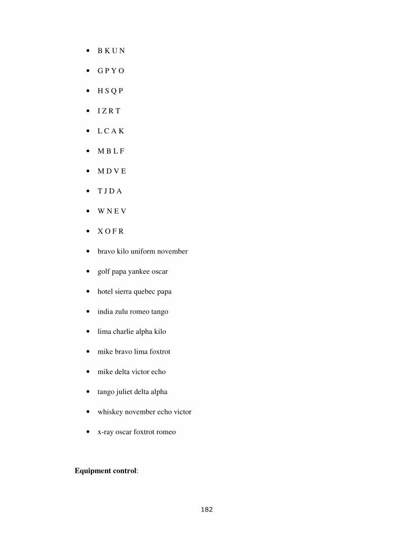
182
• B K U N
• G P Y O
• H S Q P
• I Z R T
• L C A K
• M B L F
• M D V E
• T J D A
• W N E V
• X O F R
• bravo kilo uniform november
• golf papa yankee oscar
• hotel sierra quebec papa
• india zulu romeo tango
• lima charlie alpha kilo
• mike bravo lima foxtrot
• mike delta victor echo
• tango juliet delta alpha
• whiskey november echo victor
• x-ray oscar foxtrot romeo
Equipment control:
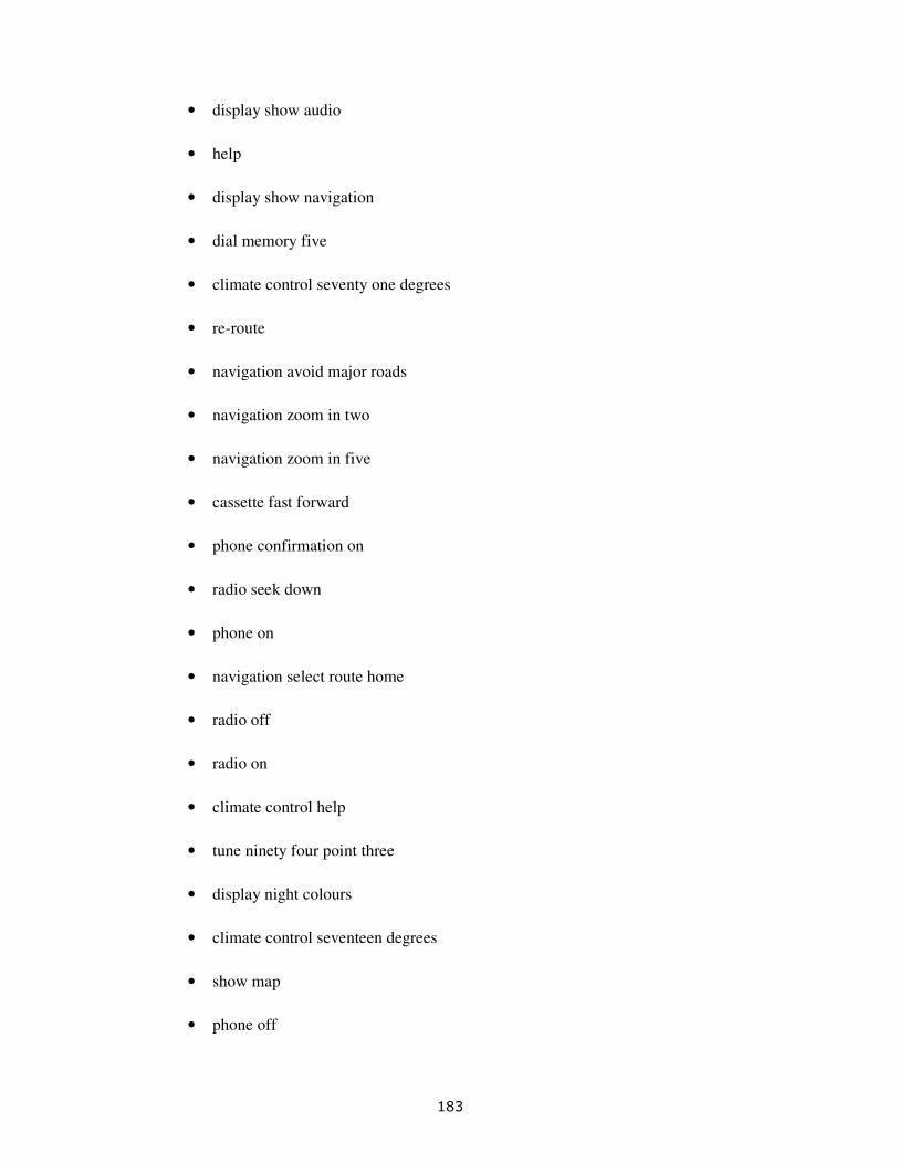
183
• display show audio
• help
• display show navigation
• dial memory five
• climate control seventy one degrees
• re-route
• navigation avoid major roads
• navigation zoom in two
• navigation zoom in five
• cassette fast forward
• phone confirmation on
• radio seek down
• phone on
• navigation select route home
• radio off
• radio on
• climate control help
• tune ninety four point three
• display night colours
• climate control seventeen degrees
• show map
• phone off

184
• tune one oh one
• changer mix tracks
• radio tune twelve fifteen medium wave
• navigation show north up
• play disc two track three
• radio tune one fifty three
• phone confirmation off
• tape dolby on
• climate recirc
• phone dial zero eight zero zero one two three nine eight seven
• phone dial zero three four five double six double seven double eight
• show present position
• navigation minimise time
• phone dial zero eight nine eight seven six five four three two one
• phone dial oh one two three four five six seven eight nine
• climate control temperature twenty three point five degrees
• phone dial oh one six eight four five eight five one one seven
Game commands:
• static
• east
• southeast
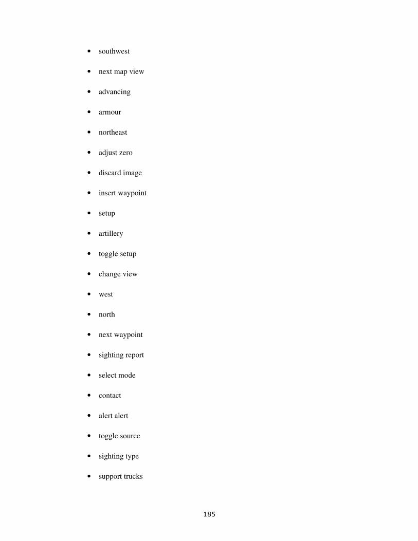
185
• southwest
• next map view
• advancing
• armour
• northeast
• adjust zero
• discard image
• insert waypoint
• setup
• artillery
• toggle setup
• change view
• west
• north
• next waypoint
• sighting report
• select mode
• contact
• alert alert
• toggle source
• sighting type
• support trucks

186
• store image
• toggle monitor
• previous waypoint
• toggle screen
• delete waypoint
• northwest
PIN numbers:
• eight four one zero
• five eight four six
• four zero nine one
• nine one five two
• one six three seven
• seven three six nine
• six two seven four
• three seven zero eight
• two five eight three
• zero nine two five

187
10.4 Pronunciation dictionary with accent features
The following pronunciation dictionary was used during the SA phase in the
experiments with accent features in Chapters 5 and 7.
A e m
A ej u
Atlantic @ t l ae n t I k u
B b 'i u
C s 'i u
D d 'i u
Drake d r e k m
Drake d r ej k u
Drake's d r e k s m
Drake's d r ej k s u
Drakes d r e k s m
Drakes d r ej k s u
E 'i u
Elizabeth I l I z @ b @ T u
Elizabethan I l I z @ b 'i T @ n u
Elizabethans I l I z @ b 'i T @ n z u
F E f u
Francis f r A n s I s u
Francis f r ae n s I s a
G dZ 'i u
Gary g ae r i u
H e tS m
H ej tS u
Hudd U d h,c
Hudd ^ d h
Hudd h ^ d u
I aj u
I'd aj d u
J dZ e m
J dZ ej u
K k e m
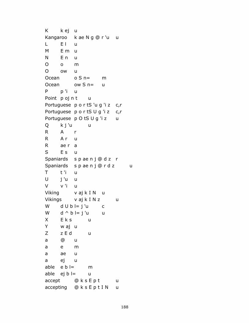
188
K k ej u
Kangaroo k ae N g @ r 'u u
L E l u
M E m u
N E n u
O o m
O ow u
Ocean o S n= m
Ocean ow S n= u
P p 'i u
Point p oj n t u
Portuguese p o r tS 'u g 'i z c,r
Portuguese p o r tS U g 'i z c,r
Portuguese p O tS U g 'i z u
Q k j 'u u
R A r
R A r u
R ae r a
S E s u
Spaniards s p ae n j @ d z r
Spaniards s p ae n j @ r d z u
T t 'i u
U j 'u u
V v 'i u
Viking v aj k I N u
Vikings v aj k I N z u
W d U b l= j 'u c
W d ^ b l= j 'u u
X E k s u
Y w aj u
Z z E d u
a @ u
a e m
a ae u
a ej u
able e b l= m
able ej b l= u
accept @ k s E p t u
accepting @ k s E p t I N u

189
access ae k s E s u
accompanied @ k U m p @ n I d c
accompanied @ k ^ m p @ n i d u
accounts @ k aw n t s u
accurate ae k j U r @ t u
across @ k r 'AO s u
action ae k S n= u
acute @ k j 'u t u
address @ d r E s u
adjust @ dZ U s t c
adjust @ dZ ^ s t u
adjusting @ dZ U s t I N c
adjusting @ dZ ^ s t I N u
advance @ d v A n s u
advance @ d v ae n s a
advanced @ d v A n s t u
advanced @ d v ae n s t a
advances @ d v A n s I z u
advances @ d v ae n s I z a
advancing @ d v A n s I N u
advancing @ d v ae n s I N a
advantage @ d v A n F I dZ f
advantage @ d v A n t I dZ u
advantage @ d v ae n F I dZ a,f
advantage @ d v ae n t I dZ a
adventure @ d v E n tS @ r
adventure @ d v E n tS @ r u
adventurers @ d v E n tS @ r @ r z u
adventurers @ d v E n tS @ r @ z r
adventurous @ d v E n tS @ r @ s u
affairs @ f e@ r z u
affairs @ f e@ z r
after A f t @ r
after A f t @ r u
after ae f t @ a,r
after ae f t @ r a
against @ g e n s t m
against @ g E n s t u
against @ g ej n s t u

190
agency e dZ @ n s i m
agency ej dZ @ n s i u
alarm @ l A m r
alarm @ l A r m u
alarm @ l ae m a,r
alarm @ l ae r m a
alert @ l 'er r t u
alert @ l 'er t r
all O l u
alleviate @ l 'i v i e t m
alleviate @ l 'i v i ej t u
allow @ l aw u
alpha ae l f @ u
alphabetic ae l f @ b E F I k f
alphabetic ae l f @ b E t I k u
alternate o l F 'er n @ t c,f
alternate o l F 'er r n @ t c,r,f
alternate o l t 'er n @ t c
alternate o l t 'er r n @ t c,r
alternate O l F 'er n @ t f
alternate O l F 'er r n @ t r,f
alternate O l F @ n e t m,f
alternate O l F @ n ej t f
alternate O l F @ r n e t m,r,f
alternate O l F @ r n ej t r,f
alternate O l t 'er n @ t r
alternate O l t 'er r n @ t u
alternate O l t @ n e t m,r
alternate O l t @ n ej t r
alternate O l t @ r n e t m
alternate O l t @ r n ej t u
an @ n u
an ae n u
and @ n d u
and ae n d u
answer A n s @ r
answer A n s @ r u
answer ae n s @ a,r
answer ae n s @ r a

191
any E n i u
are @ r
are @ r u
are A r
are A r u
armour A m @ r
armour A r m @ r u
artillery A r t I l @ r i u
artillery A t I l @ r i r
as @ z u
as ae z u
assist @ s I s t u
attacked @ t ae k t u
attitude ae F I tS 'u d f
attitude ae t I tS 'u d u
auburn o b @ n c
auburn o b @ r n c,r
auburn O b @ n r
auburn O b @ r n u
audio O d i o m
audio O d i ow u
auto o F o m,f
auto O t o m
auto O t ow u
automatic o F @ m ae F I k f
automatic O t @ m ae t I k u
autumn o F @ m c,f
autumn o t @ m c
autumn O F @ m f
autumn O t @ m u
average ae v @ r I dZ u
avoid @ v oj d u
away @ w e m
away @ w ej u
back b ae k u
balance b ae l @ n s u
barbed b A b d r
barbed b A r b d u
bass b e s m

192
bass b ae s u
bass b ej s u
batter b ae F @ r,f
batter b ae F @ r f
batter b ae t @ r
batter b ae t @ r u
be b 'i u
before b I f o c,r
before b I f o r c
before b I f O r
before b I f O r u
best b E s t u
better b E F @ f,r
better b E F @ r f
better b E t @ r
better b E t @ r u
between b I t w 'i n u
beyond b I j 'AO n d u
black b l ae k u
board b o d m,r
board b o r d m
board b O d r
board b O r d u
boats b o F s m,f
boats b o t s m
boats b ow F s f
boats b ow t s u
book b 'u k c
book b U k u
boot b 'u t u
bottom b 'AO F @ m f
bottom b 'AO t @ m u
brave b r e v m
brave b r ej v u
bravo b r A v o m
bravo b r A v ow u
brother's b r U D @ r z c
brother's b r U D @ z c,r
brother's b r ^ D @ r z u
193
brother's b r ^ D @ z r
browser b r aw z @ r
browser b r aw z @ r u
but b @ t u
but b U t c
but b ^ t u
buy b aj u
by b aj u
calculate k ae l k j 'u l e t c,m
calculate k ae l k j 'u l ej t c
calculate k ae l k j U l e t m
calculate k ae l k j U l ej t u
call k o l c
call k O l u
can k @ n u
can k ae n u
cancel k ae n s l= u
cannot k ae n 'AO t u
cartridge k A r t r I dZ u
cartridge k A t r I dZ r
cassette k @ s E t u
cat k ae t u
celebrate s E l @ b r e t m
celebrate s E l @ b r ej t u
cement s I m E n t u
center s E n F @ r,f
center s E n F @ r f
center s E n t @ r
center s E n t @ r u
centre s E n F @ r,f
centre s E n F @ r f
centre s E n t @ r
centre s E n t @ r u
change tS e n dZ m
change tS ej n dZ u
changer tS e n dZ @ m,r
changer tS e n dZ @ r m
changer tS ej n dZ @ r
changer tS ej n dZ @ r u

194
changers tS e n dZ @ r z m,r
changers tS e n dZ @ z m
changers tS ej n dZ @ z r
changers tS ej n dZ @ z u
charlie tS A l i r
charlie tS A r l i u
check tS E k u
child tS aj l d u
children tS I l d r @ n u
children's tS I l d r @ n z u
chirp tS 'er p r
chirp tS 'er r p u
classical k l ae s I k l= u
classics k l ae s I k s u
clear k l I er r
clear k l I er r u
climate k l aj m I t u
clock k l 'AO k u
close k l o s m
close k l o z m
close k l ow s u
close k l ow z u
co-operation k o 'AO p @ r e S n= m
co-operation k ow 'AO p @ r ej S n= u
colours k U l @ r z c
colours k U l @ z c,r
colours k ^ l @ r z u
colours k ^ l @ z r
combat k 'AO m b ae t u
comedies k 'AO m @ d i z u
comes k U m z c
comes k ^ m z u
command k @ m A n d u
command k @ m ae n d a
commanders k @ m A n d @ r z u
commanders k @ m A n d @ z r
commanders k @ m ae n d @ r z a
commanders k @ m ae n d @ z a,r
commandments k @ m A n d m @ n t s u

195
commandments k @ m ae n d m @ n t s a
commandos k @ m A n d o z m
commandos k @ m A n d ow z u
commandos k @ m ae n d o z a,m
commandos k @ m ae n d ow z a
competence k 'AO m p I F @ n s f
competence k 'AO m p I t @ n s u
complete k @ m p l 'i t u
compress k 'AO m p r E s u
compression k @ m p r E S n= u
conditions k @ n d I S n= z u
confidence k 'AO n f I d n= s u
confirm k @ n f 'er m r
confirm k @ n f 'er r m u
confirmation k 'AO n f @ m e S n= m
confirmation k 'AO n f @ m ej S n= u
connect k @ n E k t u
contact k O n t ae k t u
contagious k @ n t e dZ @ s m
contagious k @ n t ej dZ @ s u
contract k @ n t r ae k t u
contract k 'AO n t r ae k t u
contrast k @ n t r A s t u
contrast k @ n t r ae s t a
contrast k 'AO n t r A s t u
contrast k 'AO n t r ae s t a
control k @ n t r o l m
control k @ n t r ow l u
cook k 'u k c
cook k U k u
cooked k 'u k t c
cooked k U k t u
country k U n t r I c
country k ^ n t r i u
course k O r s u
course k O s r
courtesy k 'er F @ s i r,f
courtesy k 'er r F @ s i f
courtesy k 'er r t @ s i u

196
courtesy k 'er t @ s i r
crab k r ae b u
craft k r A f t u
craft k r ae f t a
crew k r 'u u
crews k r 'u z u
cubic k j 'u b I k u
cultured k U l tS @ d c,r
cultured k U l tS @ r d c
cultured k ^ l tS @ d r
cultured k ^ l tS @ r d u
current k U F @ n t c,f
current k U r @ n t c
current k ^ F @ n t f
current k ^ r @ n t u
cursor k 'er r s @ r u
cursor k 'er s @ r
danger d e n dZ @ m,r
danger d e n dZ @ r m
danger d ej n dZ @ r
danger d ej n dZ @ r u
day d e m
day d ej u
deadline d E d l aj n u
decrease d 'i k r 'i s u
decrease d I k r 'i s u
deed d 'i d u
deeds d 'i d z u
default d I f O l t u
degrees d I g r 'i z u
delete d I l 'i t u
delta d E l F @ f
delta d E l t @ u
demist d 'i m I s t u
despite d I s p aj t u
destination d E s t I n e S n= m
destination d E s t I n ej S n= u
detail d 'i t e l m
detail d 'i t ej l u

197
determination d I t 'er m I n e S n= m,r
determination d I t 'er m I n ej S n= r
determination d I t 'er r m I n e S n= m
determination d I t 'er r m I n ej S n= u
detour d 'i t 'u @ c,r
detour d 'i t 'u r c
detour d 'i t U @ r
detour d 'i t U @ r u
dial d aj @ l u
did d I d u
directory d I r E k t @ r i u
directory d aj r E k t @ r i u
disallow d I s @ l aw u
disappeared d I s @ p I er d r
disappeared d I s @ p I er r d u
disc d I s k u
discard d I s k A d r
discard d I s k A r d u
discharge d I s tS A dZ r
discharge d I s tS A r dZ u
discs d I s k s u
diseases d I z 'i z I z u
dispense d I s p E n s u
dispensed d I s p E n s t u
dispensing d I s p E n s I N u
dispersed d I s p 'er r s t u
dispersed d I s p 'er s t r
display d I s p l e m
display d I s p l ej u
dispute d I s p j 'u t u
distance d I s t @ n s u
distant d I s t @ n t u
document d 'AO k j 'u m @ n t c
document d 'AO k j 'u m E n t c
document d 'AO k j U m @ n t u
document d 'AO k j U m E n t u
documentary d 'AO k j 'u m E n t r i c
documentary d 'AO k j U m E n t r i u
dolby d 'AO l b i u

198
doors d o r z c
doors d o s c,r
doors d O r z u
doors d O z r
double d U b l= c
double d ^ b l= u
down d aw n u
drama d r A m @ u
drink d r I N k u
driver d r aj v @ r
driver d r aj v @ r u
each 'i tS u
easier 'i z i @ r
easier 'i z i @ r u
east 'i s t u
easy 'i z i u
echo e k o m
echo E k ow u
economy I k 'AO n @ m i u
educate E dZ 'u k e t c,m
educate E dZ 'u k ej t c
educate E dZ U k e t m
educate E dZ U k ej t u
education E dZ 'u k e S n= c,m
education E dZ 'u k ej S n= c
education E dZ U k e S n= m
education E dZ U k ej S n= u
eight e t m
eight ej t u
eighteen e t 'i n m
eighteen ej t 'i n u
eighty e F i m,f
eighty e t i m
eighty ej F i f
eighty ej t i u
eject I dZ E k t u
eleven I l E v n= u
emergency I m 'er dZ @ n s i r
emergency I m 'er r dZ @ n s i u

199
en-route E n r 'u t u
en-route E n r aw t u
end E n d u
enough I n U f c
enough I n ^ f u
enter E n F @ r,f
enter E n F @ r f
enter E n t @ r
enter E n t @ r u
equipment I k w I p m @ n t u
error E r @ r
error E r @ r u
even 'i v n= u
evening 'i v n I N u
ever E v @ r
ever E v @ r u
exploits E k s p l oj t s u
exploits I k s p l oj t s u
exposure I k s p ow Z u
exposures I k s p ow Z z u
external I k s t 'er n l= u
extra E k s t r @ u
faced f e s t m
faced f ej s t u
faces f e s I z m
faces f ej s I z u
fact f ae k t u
fade f e d m
fade f ej d u
faith f e T m
faith f ej T u
fame f e m m
fame f ej m u
fan f ae n u
far f A r
far f A r u
fast f A s t u
fast f ae s t a
father f A D @ r

200
father f A D @ r u
father f ae D @ a,r
father f ae D @ r a
favour f e v @ m,r
favour f e v @ r m
favour f ej v @ r
favour f ej v @ r u
fed f E d u
feedback f 'i d b ae k u
female f 'i m e l m
female f 'i m ej l u
few f j 'u u
field f 'i l d u
fifteen f I f t 'i n u
fifty f I f F i f
fifty f I f t i u
filler f I l @ r
filler f I l @ r u
finance f aj n ae n s u
fine f aj n u
fire f aj @ r
fire f aj r u
firebooters f aj @ b 'u t @ z r
firebooters f aj b 'u F @ z r,f
firebooters f aj r b 'u F @ r z f
firebooters f aj r b 'u t @ r z u
firm f 'er m r
firm f 'er r m u
first f 'er r s t u
first f 'er s t r
five f aj v u
flap f l ae p u
flavour f l e v @ m,r
flavour f l e v @ r m
flavour f l ej v @ r
flavour f l ej v @ r u
fleet f l 'i t u
fleets f l 'i t s u
floor f l o c,r

201
floor f l o r c
floor f l O r
floor f l O r u
folk f o k m
folk f ow k u
food f 'u d u
fools f 'u l z u
foot f 'u t c
foot f U t u
for f @ u
for f o c,r
for f o r c
for f O r
for f O r u
forty f o F i c,r,f
forty f o r F i c,f
forty f o r t i c
forty f o t i c,r
forty f O F i r,f
forty f O r F i f
forty f O r t i u
forty f O t i r
forward f o r w @ r d c
forward f o w @ d c,r
forward f O r w @ r d u
forward f O w @ d r
found f aw n d u
four f o c,r
four f o r c
four f O r
four f O r u
fourteen f o r t 'i n c
fourteen f o t 'i n c,r
fourteen f O r t i n u
fourteen f O t 'i n r
foxtrot f 'AO k s t r 'AO t u
freebooters f r 'i b 'u F @ r z f
freebooters f r 'i b 'u F @ z r,f
freebooters f r 'i b 'u t @ r z u

202
freebooters f r 'i b 'u t @ z r
frequency f r 'i k w @ n s i u
from f r @ m u
from f r 'AO m u
front f r U n t c
front f r ^ n t u
fructose f r U k t o z c,m
fructose f r ^ k t o z c
fructose f r ^ k t o z m
fructose f r ^ k t ow z u
fruit f r 'u t u
fruits f r 'u t s u
fuel f j 'u @ l u
further f 'er D @ r
further f 'er r D @ r u
gas g ae s u
gate g e t m
gate g ej t u
gave g e v m
gave g ej v u
generally dZ E n r @ l i u
generates dZ E n @ r e t s m
generates dZ E n @ r ej t s u
generation dZ E n @ r e S n= m
generation dZ E n @ r ej S n= u
generations dZ E n @ r e S n= z m
generations dZ E n @ r ej S n= z u
give g I v u
glory g l o r i c
glory g l O r i u
glucose g l 'u k o s m
glucose g l 'u k ow s u
go g o m
go g ow u
god g 'AO d u
gods g 'AO d z u
golf g 'AO l f u
good g 'u d c
good g U d u

203
goods g 'u d z c
goods g U d z u
grab g r ae b u
grabs g r ae b z u
great g r e t m
great g r ej t u
guidance g aj d n= s u
guide g aj d u
guided g aj d I d u
had @ d h
had ae d h
had h @ d u
had h ae d u
hade e d h,m
hade ej d h
hade h e d m
hade h ej d u
hair e@ h
hair h e@ r
hair h e@ r u
half A f h
half h A f u
hard A d h
hard A d h,r
hard h A d r
hard h A d u
hared e@ d h,r
hared e@ r d h
hared h e@ d r
hared h e@ r d u
has @ z h
has ae z h
has h @ z u
has h ae z u
hash ae S h
hash h ae S u
hate e t h,m
hate ej t h
hate h e t m

204
hate h ej t u
have @ v h
have ae v h
have h @ v u
have h ae v u
he 'i h
he h 'i u
he's 'i z h
he's I z h
he's h 'i z u
he's h I z u
head E d h
head h E d u
hear I er h,r
hear I er r h
hear h I er r
hear h I er r u
heard 'er d h,r
heard 'er r d h
heard h 'er d r
heard h 'er r d u
heated 'i F I d h,f
heated 'i t I d h
heated h 'i F I d f
heated h 'i t I d u
heed 'i d h
heed h 'i d u
heered I er d h,r
heered I er r d h
heered h I er d r
heered h I er r d u
heighten aj F @ n h,f
heighten aj t @ n h
heighten h aj F @ n f
heighten h aj t @ n u
heightened aj F @ n d h
heightened aj F @ n d h,f
heightened h aj F @ n d f
heightened h aj t @ n d u

205
heightening aj F @ n I N h,f
heightening aj t @ n I N h
heightening h aj F @ n I N f
heightening h aj t @ n I N u
held E l d h
held h E l d u
help E l p h
help h E l p u
helping E l p I N h
helping h E l p I N u
her 'er h,r
her 'er r h
her h 'er r
her h 'er r u
hid I d h
hid h I d u
hide aj d h
hide h aj d u
high aj h
high h aj u
higher aj @ h,r
higher aj @ r h
higher h aj @ r
higher h aj @ r u
him I m h
him h I m u
his I z h
his h I z u
hoard o d c,h,r
hoard o r d c,h
hoard h o d c,r
hoard h o r d c
hoard h O d r
hoard h O r d u
hoard O d h,r
hoard O r d h
hobby h 'AO b i u
hobby 'AO b i h
hod h 'AO d u

206
hod 'AO d h
hoed o d h,m
hoed h o d m
hoed h ow d u
hoed ow d h
hoid h oj d u
hoid oj d h
hold o l d h,m
hold h o l d m
hold h ow l d u
hold ow l d h
home o m h,m
home h o m m
home h ow m u
home ow m h
hood 'u d c,h
hood U d h
hood h 'u d c
hood h U d u
horn o n c,h,r
horn o r n c,h
horn h o n c,r
horn h o r n c
horn h O n r
horn h O r n u
horn O r n h
hotel o t e l h,m
hotel h o t e l m
hotel h ow t E l u
hotel ow t E l h
hour aw @ r
hour aw @ r u
howd aw d h
howd h aw d u
hundred U n d r @ d c,h
hundred ^ n d r @ d h
hundred h U n d r @ d c
hundred h ^ n d r @ d u
hurled 'er l d h,r

207
hurled 'er r l d h
hurled h 'er l d r
hurled h 'er r l d u
image I m I dZ u
improved I m p r 'u v d u
in I n u
increase I n k r 'i s u
india I n d i @ u
info I n f o m
info I n f ow u
information I n f @ m e S n= m,r
information I n f @ m ej S n= r
information I n f @ r m e S n= m
information I n f @ r m ej S n= u
insert I n s 'er r t u
insert I n s 'er t r
instant I n s t @ n t u
instrument I n s t r @ m @ n t u
instrument I n s t r @ m E n t u
instruments I n s t r @ m @ n t s u
instruments I n s t r @ m E n t s u
interest I n t r @ s t u
interior I n t I er r i @ u
iota aj ow t @ u
is I z u
it I t u
it's I t s u
itemise aj F @ m aj z f
itemise aj t @ m aj z u
jazz dZ ae z u
juliet dZ 'u l i E t c
juliet dZ U l i E t u
junction dZ U N k S n= c
junction dZ ^ N k S n= u
kilo k 'i l o m
kilo k 'i l ow u
kilometres k I l @ m 'i F @ r z f
kilometres k I l @ m 'i F @ z r,f
kilometres k I l @ m 'i t @ r z u

208
kilometres k I l @ m 'i t @ z r
kilometres k I l 'AO m I F @ r z f
kilometres k I l 'AO m I F @ z r,f
kilometres k I l 'AO m I t @ r z u
kilometres k I l 'AO m I t @ z r
knowledge n 'AO l I dZ u
land l ae n d u
lands l ae n d z u
later l e F @ m,r,f
later l e F @ r m,f
later l e t @ m,r
later l e t @ r m
later l ej F @ r,f
later l ej F @ r f
later l ej t @ r
later l ej t @ r u
leaves l 'i v z u
left l E f t u
leisure l E Z u
less l E s u
level l E v l= u
lift l I f t u
light l aj t u
lights l aj t s u
lima l 'i m @ u
list l I s t u
listening l I s n= I N u
little l I F l= f
little l I t l= u
live l I v u
live l aj v u
load l o d m
load l ow d u
loathe l o D m
loathe l ow D u
loathed l o D d m
loathed l ow D d u
local l o k @ l m
local l ow k @ l u

209
location l o k e S n= m
location l ow k ej S n= u
lock l 'AO k u
locks l 'AO k s u
long l 'AO N u
look l 'u k c
look l U k u
looked l 'u k t c
looked l U k t u
looking l 'u k I N c
looking l U k I N u
loud l aw d u
low l o m
low l ow u
lower l o @ m,r
lower l o @ r m
lower l ow @ r
lower l ow @ r u
mac m ae k u
made m e d m
made m ej d u
magazine m ae g @ z 'i n u
major m e dZ @ m,r
major m e dZ @ r m
major m ej dZ @ r
major m ej dZ @ r u
make m e k m
make m ej k u
makes m e k s m
makes m ej k s u
male m e l m
male m ej l u
map m ae p u
mat m ae t u
maximum m ae k s I m @ m u
may m e m
may m ej u
me m 'i u
meanings m 'i n I N z u

210
means m 'i n z u
meant m E n t u
measure m E Z u
measured m E Z d r
measured m E Z r d u
measuring m E Z r I N u
media m 'i d i @ u
medicine m E d s n= u
medicines m E d s n= z u
medium m 'i d i @ m u
meet m 'i t u
member m E m b @ r
member m E m b @ r u
members m E m b @ r z u
members m E m b @ z r
memory m E m @ F i u
memory m E m @ r i r
men m E n u
menu m E n j 'u u
message m E s I dZ u
met m E t u
metric m E t r I k u
middle m I d l= u
might m aj t u
mighty m aj F i f
mighty m aj t i u
mike m aj k u
miles m aj l z u
milk m I l k u
millenium m I l E n i @ m u
millennium m I l E n i @ m u
million m I l i @ n u
minidisc m I n i d I s k u
minimise m I n I m aj z u
minimum m I n I m @ m u
minor m aj n @ r
minor m aj n @ r u
mirage m I r A Z u
mirror m I r @ r

211
mirror m I r @ r u
mirrors m I r @ r z u
mirrors m I r @ z r
mix m I k s u
mixer m I k s @ r
mixer m I k s @ r u
mode m o d m
mode m ow d u
model m 'AO d l= u
modern m 'AO d er n= r
modern m 'AO d n= u
modest m 'AO d I s t u
monitor m 'AO n I F @ f
monitor m 'AO n I F @ r r,f
monitor m 'AO n I t @ u
monitor m 'AO n I t @ r r
more m o m,r
more m o r m
more m O r
more m O r u
most m o s t m
most m ow s t u
motorway m o F @ r w e m,f
motorway m o F @ w e m,r,f
motorway m o t @ r w e m
motorway m o t @ w e m,r
motorway m ow F @ r w ej f
motorway m ow F @ w ej r,f
motorway m ow t @ r w ej u
motorway m ow t @ w ej r
mouse m aw s u
music m j 'u z I k u
mute m j 'u t u
my m aj u
national n ae S n l= u
natural n ae tS r @ l u
navigate n ae v I g e t m
navigate n ae v I g ej t u
navigation n ae v I g e S n= m

212
navigation n ae v I g ej S n= u
navigational n ae v I g e S n= @ l m
navigational n ae v I g ej S n= @ l u
navigations n ae v I g e S n= z m
navigations n ae v I g ej S n= z u
need n 'i d u
needs n 'i d z u
never n E v @ r
never n E v @ r u
new n j 'u u
news n j 'u z u
next n E k s t u
night n aj t u
nine n aj n u
nineteen n aj n t 'i n u
ninety n aj n F i f
ninety n aj n t i u
no n o m
no n ow u
none n U n c
none n ^ n u
normal n o m l= c,r
normal n o r m l= c
normal n O m l= r
normal n O r m l= u
north n o T c,r
north n o r T c
north n O T r
north n O r T u
northeast n o T i s t c,r
northeast n o r T i s t c
northeast n O T 'i s t r
northeast n O r T i s t u
northwest n o T w E s t c,r
northwest n o r T w E s t c
northwest n O T w E s t r
northwest n O r T w E s t u
not n 'AO t u
nothing n U T I N c

213
nothing n ^ T I N u
nought n O t u
november n o v e m b @ m,r
november n o v e m b @ r m
november n ow v E m b @ r
november n ow v E m b @ r u
numbers n U m b @ r z c
numbers n U m b @ z c,r
numbers n ^ m b @ r z u
numbers n ^ m b @ z r
o'clock @ k l 'AO k u
oafs o f s m
oafs ow f s u
oarmen o m @ n c,r
oarmen o r m @ n c
oarmen O m @ n r
oarmen O r m @ n u
oars o r z c
oars o z c,r
oars O r z u
oars O z r
oarsmen o r z m @ n c
oarsmen o z m @ n c,r
oarsmen O r z m @ n u
oarsmen O z m @ n r
oarsmens o r z m @ n z c
oarsmens o z m @ n z c,r
oarsmens O r z m @ n z u
oarsmens O z m @ n z r
oasis o e s I s m
oasis ow ej s I s u
ocean o S n= m
ocean ow S n= u
of @ v u
of O v u
off O f u
official @ f I S l= u
often O f F @ n f
often O f n= u

214
often O f t @ n u
oh o m
oh ow u
ok o k e m
ok ow k ej u
oldies o l d i z m
oldies ow l d i z u
on O n u
one w U n c
one w ^ n u
open o p @ n m
open ow p @ n u
option O p S n= u
or @ r
or @ r u
or o c,r
or o r c
or O r
or O r u
oscar O s k @ r
oscar O s k @ r u
ot O t u
other U D @ c,r
other U D @ r c
other ^ D @ r
other ^ D @ r u
our aw @ r
our aw @ r u
out aw t u
outside aw t s aj d u
over o v @ m
over o v @ r m,r
over ow v @ r
over ow v @ r u
overlooked o v @ l 'u k t c,m,r
overlooked o v @ l U k t m,r
overlooked o v @ r l 'u k t c,m
overlooked o v @ r l U k t m
overlooked ow v @ l 'u k t c,r

215
overlooked ow v @ l U k t r
overlooked ow v @ r l 'u k t c
overlooked ow v @ r l U k t u
own o n m
own ow n u
page p e dZ m
page p ej dZ u
pair p e@ r
pair p e@ r u
papa p @ p A u
papa p @ p ae a
parking p A k I N r
parking p A r k I N u
passenger p ae s I n dZ @ r
passenger p ae s I n dZ @ r u
pause p o z c
pause p O z u
people p 'i p l= u
percent p @ r s E n t u
percent p @ s E n t r
petrol p E t r @ l u
phone f o n m
phone f ow n u
plan p l ae n u
platoon p l @ t 'u n u
play p l e m
play p l ej u
plus p l U s c
plus p l ^ s u
point p oj n t u
points p oj n t s u
pop p 'AO p u
position p @ z I S n= u
postponed p o s p o n d m
postponed p ow s p ow n d u
powered p aw @ d r
powered p aw @ r d u
practice p r ae k t I s u
prefer p r I f 'er r

216
prefer p r I f 'er r u
preference p r E f @ r @ n s u
presence p r E z n= s u
present p r E z n= t u
present p r I z E n t u
preset p r 'i s E t u
presets p r 'i s E t s u
pressure p r E S u
previous p r 'i v i @ s u
prison p r I z n= u
profound p r @ f aw n d u
programs p r o g r ae m z m
programs p r ow g r ae m z u
project p r @ dZ E k t u
project p r 'AO dZ E k t u
protecting p r @ t E k t I N u
protection p r @ t E k S n= u
puddings p 'u d I N z c
puddings p U d I N z u
pulling p 'u l I N c
pulling p U l I N u
quebec k w I b E k u
quickly k w I k l i u
radio r e d i o m
radio r ej d i ow u
random r ae n d @ m u
re-route r 'i r 'u t u
reached r 'i tS t u
read r 'i d u
read r E d u
rear r I er u
reassurance r 'i @ S 'u r @ n s c
reassurance r 'i @ S U @ r @ n s u
reassuring r 'i @ S 'u r I N c
reassuring r 'i @ S U @ r I N u
rec r E k u
recall r I k O l u
recce r E k i u
receive r I s 'i v u

217
received r I s 'i v d u
recent r 'i s n= t u
recirc r 'i s 'er k r
recirc r 'i s 'er r k u
recognition r E k @ g n I S n= u
recur r I k 'er r
recur r I k 'er r u
redial r 'i d aj @ l u
reduce r I d j 'u s u
reduced r I d j 'u s t u
reducing r I d j 'u s I N u
release r I l 'i s u
reliable r I l aj @ b l= u
reliance r I l aj @ n s u
reliant r I l aj @ n t u
religion r I l I dZ @ n u
remaining r I m e n I N m
remaining r I m ej n I N u
remembered r I m E m b @ d r
remembered r I m E m b @ r d u
reminded r I m aj n d I d u
repeat r I p 'i t u
report r I p o r t c,r
report r I p o t c
report r I p O t u
reroute r 'i r 'u t u
research r 'i s 'er r tS u
research r 'i s 'er tS r
research r I s 'er r tS u
research r I s 'er tS r
researched r 'i s 'er r tS t u
researched r 'i s 'er tS t r
researched r I s 'er r tS t u
researched r I s 'er tS t r
reset r 'i s E t u
restrict r I s t r I k t u
return r I t 'er n r
return r I t 'er r n u
reveal r I v 'i l u

218
reverse r I v 'er r s u
reverse r I v 'er s r
rewind r 'i w aj n d u
ride r aj d u
right r aj t u
risk r I s k u
risks r I s k s u
road r o d m
road r ow d u
roads r o d z m
roads r ow d z u
rock r 'AO k u
roll r o l m
roll r ow l u
romeo r o m i o m
romeo r ow m i ow u
room r 'u m u
rose r o z m
rose r ow z u
route r 'u t u
routes r 'u t s u
sail s e l m
sail s ej l u
sailor s e l @ m,r
sailor s e l @ r m
sailor s ej l @ r
sailor s ej l @ r u
same s e m m
same s ej m u
save s e v m
save s ej v u
scale s k e l m
scale s k ej l u
scampered s k ae m p @ d r
scampered s k ae m p @ r d u
scan s k ae n u
scene s 'i n u
science s aj @ n s u
screen s k r 'i n u

219
scroll s k r o l m
scroll s k r ow l u
search s 'er r tS u
search s 'er tS r
seat s 'i t u
seats s 'i t s u
section s E k S n= u
security s I k j 'u f @ F i c,f
security s I k j 'u r @ t i c
security s I k j U @ r @ t i u
security s I k j U f @ F i f
seek s 'i k u
seems s 'i m z u
select s I l E k t u
selection s I l E k S n= u
self-handed s E l f ae n d I d h
self-handed s E l f h ae n d I d u
self-steering s E l f s t I er r I N u
send s E n d u
serious s I er r i @ s u
set s E t u
setting s E F I N f
setting s E t I N u
setup s E F U p c,f
setup s E F ^ p f
setup s E t U p c
setup s E t ^ p u
seven s E v n= u
seventeen s E v n= t 'i n u
seventy s E v n= F i f
seventy s E v n= t i u
she S 'i u
she's S 'i z u
she's S I z u
ship S I p u
ships S I p s u
should S 'u d c
should S U d u
show S o m

220
show S ow u
shown S o n m
shown S ow n u
shows S o z m
shows S ow z u
shuffle S U f l= c
shuffle S ^ f l= u
side s aj d u
sides s aj d z u
sierra s i e@ r @ u
sight s aj t u
sighting s aj F I N f
sighting s aj t I N u
sightings s aj F I N z f
sightings s aj t I N z u
single s I N g l= u
single-handed s I N g l= ae n d I d h
single-handed s I N g l= h ae n d I d u
sister s I s t @ r
sister s I s t @ r u
sister-ships s I s t @ S I p s r
sister-ships s I s t @ r S I p s u
sisters s I s t @ r z u
sisters s I s t @ z r
six s I k s u
sixteen s I k s t 'i n u
sixty s I k s F i f
sixty s I k s t i u
size s aj z u
slighting s l aj F I N f
slighting s l aj t I N u
slightly s l aj F l i f
slightly s l aj t l i u
slowly s l o l i m
slowly s l ow l i u
small s m o l c
small s m O l u
smaller s m o l @ c,r
smaller s m o l @ r c

221
smaller s m O l @ r
smaller s m O l @ r u
so s o m
so s ow u
social s o S l= m
social s ow S l= u
soft s 'AO f t u
some s U m c
some s ^ m u
sounds s aw n d z u
source s o r s c
source s o s c,r
source s O r s u
source s O s r
southeast s aw T 'i s t u
southwest s aw T w E s t u
speech s p 'i tS u
speed s p 'i d u
split s p l I t u
sport s p o r t c
sport s p o t c,r
sport s p O r t u
sport s p O t r
stable s t e b l= m
stable s t ej b l= u
star s t A r
star s t A r u
stars s t A r z u
stars s t A z r
static s t ae F I k f
static s t ae t I k u
stations s t e S n= z m
stations s t ej S n= z u
steering s t I er r I N u
stem s t E m u
stems s t E m z u
stop s t 'AO p u
storage s t o r I dZ c
storage s t O r I dZ u

222
store s t o c
store s t o r c,r
store s t O r
store s t O r u
strong s t r 'AO N u
stronger s t r 'AO N g @ u
stronger s t r 'AO N g @ r r
success s @ k s E s u
sugars S 'u g @ r z c
sugars S 'u g @ z c,r
sugars S U g @ r z u
sugars S U g @ z r
suitable s 'u F @ b l= f
suitable s 'u t @ b l= u
supplied s @ p l aj d u
supplies s @ p l aj z u
support s @ p o r t c
support s @ p o t c,r
support s @ p O r t u
support s @ p O t r
surrounded s @ r aw n d I d u
sweet s w 'i t u
switch s w I tS u
system s I s t @ m u
taken t e k @ n m
taken t ej k @ n u
takes t e k s m
takes t ej k s u
tango t ae N g o m
tango t ae N g ow u
tape t e p m
tape t ej p u
tea t 'i u
team t 'i m u
teletext t E l I t E k s t u
temperature t E m p r @ tS @ r
temperature t E m p r @ tS @ r u
temperatures t E m p r @ tS @ r z u
temperatures t E m p r @ tS @ z r

223
ten t E n u
test t E s t u
than D @ n u
than D ae n u
thanks T ae N k s u
that D @ t u
that D ae t u
the D 'i u
the D @ u
their D e@ r
their D e@ r u
them D @ m u
them D E m u
themselves D E m s E l v z u
there D e@ r
there D e@ r u
these D 'i z u
they D e m
they D ej u
thin T I n u
thirteen T 'er r t 'i n u
thirteen T 'er t 'i n r
thirty T 'er F i r,f
thirty T 'er r F i f
thirty T 'er r t i u
thirty T 'er t i r
this D I s u
thought T O t u
thoughts T O t s u
three T F 'i f
three T r 'i u
time t aj m u
tip t I p u
to t 'u u
to t @ u
today t @ d e m
today t @ d ej u
todays t @ d e z m
todays t @ d ej z u

224
toggle t 'AO g l= u
toggling t 'AO g l= I N u
toll t o l m
toll t ow l u
took t 'u k c
took t U k u
tools t 'u l z u
top t 'AO p u
total t o F l= m,f
total t o t l= m
total t ow F l= f
total t ow t l= u
touch t U tS c
touch t ^ tS u
touring t 'u @ r I N c
touring t U @ r I N u
trace t r e s m
trace t r ej s u
track t r ae k u
tracks t r ae k s u
traction t r ae k S n= u
traffic t r ae f I k u
train t r e n m
train t r ej n u
transit t r ae n z I t u
transmit t r ae n z m I t u
travel t r ae v l= u
treble t r E b l= u
trip t r I p u
trucks t r U k s c
trucks t r ^ k s u
trust t r U s t c
trust t r ^ s t u
truth t r 'u T u
tune t j 'u n u
turn t 'er n r
turn t 'er r n u
tweezers t w 'i z @ r z u
tweezers t w 'i z @ z r

225
twelve t w E l v u
twenty t w E n F i f
twenty t w E n t i u
two t 'u u
type t aj p u
unbeatable U n b 'i F @ b l= c,f
unbeatable U n b 'i t @ b l= c
unbeatable ^ n b 'i F @ b l= f
unbeatable ^ n b 'i t @ b l= u
understanding U n d @ r s t ae n d I N c
understanding U n d @ s t ae n d I N c,r
understanding ^ n d @ r s t ae n d I N u
understanding ^ n d @ s t ae n d I N r
undue U n d j 'u c
undue ^ n d j 'u u
uniform j 'u n I f o m c,r
uniform j 'u n I f o r m c
uniform j 'u n I f O m r
uniform j 'u n I f O r m u
unlock U n l 'AO k c
unlock ^ n l 'AO k u
unmistakable U n m I s t e k @ b l= c,m
unmistakable U n m I s t ej k @ b l= c
unmistakable ^ n m I s t e k @ b l= m
unmistakable ^ n m I s t ej k @ b l= u
unshakeable U n S e k @ b l= c,m
unshakeable U n S ej k @ b l= c
unshakeable ^ n S e k @ b l= m
unshakeable ^ n S ej k @ b l= u
up U p c
up ^ p u
varied v e@ r i d u
vast v A s t u
vast v ae s t a
veered v I er d r
veered v I er r d u
vehicle v 'i I k l= u
vehicles v 'i I k l= z u
vent v E n t u

226
vents v E n t s u
venture v E n tS @ r
venture v E n tS @ r u
verbal v 'er b l= r
verbal v 'er r b l= u
version v 'er S n= r
version v 'er r S n= u
versions v 'er S n= z r
versions v 'er r S n= z u
victor v I k t @ r
victor v I k t @ r u
victory v I k t @ r i u
view v j 'u u
villains v I l @ n z u
vision v I Z n= u
visions v I Z n= z u
voice v oj s u
volume v 'AO l j 'u m u
wafer w e f @ m
wafer w e f @ r m,r
wafer w ej f @ u
wall w o l c
wall w O l u
was w @ z u
was w 'AO z u
watch w 'AO tS u
water w o F @ c,r,f
water w o F @ r c,f
water w o t @ c,r
water w o t @ r c
water w O F @ r,f
water w O F @ r f
water w O t @ r
water w O t @ r u
wave w e v m
wave w ej v u
way w e m
way w ej u
waypoint w e p oj n t m

227
waypoint w ej p oj n t u
wayward w e w @ d m,r
wayward w e w @ r d m
wayward w ej w @ d r
wayward w ej w @ r d u
we w 'i u
we're w I er r
we're w I er r u
we've w 'i v u
weather w E D @ r
weather w E D @ r u
weathers w E D @ r z u
weathers w E D @ z r
were w 'er r
were w 'er r u
were w @ r
were w @ r u
west w E s t u
what w 'AO t u
when w E n u
where w e@ r
where w e@ r u
which w I tS u
while w aj l u
whiskey w I s k i u
who 'u h
who h 'u u
who'd 'u d h
who'd h 'u d u
will w I l u
wind w I n d u
wind w aj n d u
window w I n d o m
window w I n d ow u
windows w I n d o z m
windows w I n d ow z u
windscreen w I n d s k r 'i n u
wire w aj @ r
wire w aj er u

228
with w I D u
withdrawing w I D d r o I N c
withdrawing w I D d r O I N u
withdrawn w I D d r o n c
withdrawn w I D d r O n u
worry w U r i c
worry w ^ r i u
x-ray E k s r e m
x-ray E k s r ej u
yacht j 'AO t u
yankee j ae N k i u
yards j A d z r
yards j A r d z u
years j I er r z u
years j I er z r
yell j E l u
yes j E s u
you j 'u u
young j U N c
young j ^ N u
your j 'u @ c,r
your j 'u r c
your j U @ r u
your j U @ r
your j O r
your j O r u
zero z I er r ow u
zone z o n m
zone z ow n u
zoom z 'u m u
zulu z 'u l 'u u

229
10.5 List of publications
”Using Accent Dictionaries in Automatic Speech Recognition”, Tjalve 2003
Alumni Reunion Conference 2003, University College London
”Accent Features for Pronunciation Dictionary Adaptation in ASR”, Tjalve 2004a
CamLing Conference 2004, Cambridge University
”Phonological Adaptation using Accent Features in Automatic Speech Recognition”,
Tjalve 2004b
Speech Hearing and Language 2004
”How to Build an Italian Speech Recogniser without Italian Speech Data”, Tjalve
2005a
PhD Day, UCL, 2005
”Pronunciation Variation Modelling using Accent Features”, Tjalve 2005b
Proceedings of Eurospeech, Lisbon, Portugal, 2005
”Non-Native Speech Recognition Empowered by Linguistic Fusion”, Tjalve 2005c
Technical Report, Infinitive Speech Systems, 2005

230
”What Speech Technology Can Teach Us about Accent Variation”, Tjalve 2006a
British Accent Seminar, UCL, 2006

231