The multiplier-accelerator model

Initial points

1. The model is a synthesis of the Kahn-Keynes multiplier and the “accelerator” theory of investment1.

2. The accelerator model is based on the truism that, if technology (and thus the capital/output ratio) is held constant, an increase in output can only be achieved though an increase in the capital stock.

P. Samuelson. “Interaction Between the Multiplier Analysis and the Principle of Acceleration,” Review of Economic Statistics (May 1939).

The accelerator

•Firms need a given quantity of capital to produce the current level of output. If the level of output changes, they will need more capital. How much more?

Change in capital = accelerator × change in output (10.1)

•But firms can only increase their capital stock by (positive) net investment. How much?

Net investment = accelerator × change in output (10.2)

•It is also true that:

Accelerator = Change in Capital/Change in Output

Capital/Output ratio

•If we do not allow for productivity boosting technical change, then the capital output ratio is held constant.

•If fact, this is what we are assuming—no technical change.

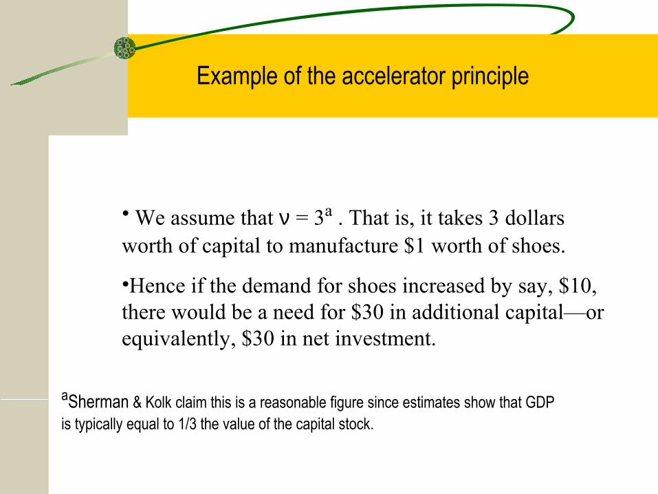
Example of the accelerator principle

aSherman & Kolk claim this is a reasonable figure since estimates show that GDP is typically equal to 1/3 the value of the capital stock.

• We assume that ν = 3a . That is, it takes 3 dollars worth of capital to manufacture $1 worth of shoes.

•Hence if the demand for shoes increased by say, $10, there would be a need for $30 in additional capital—or equivalently, $30 in net investment.

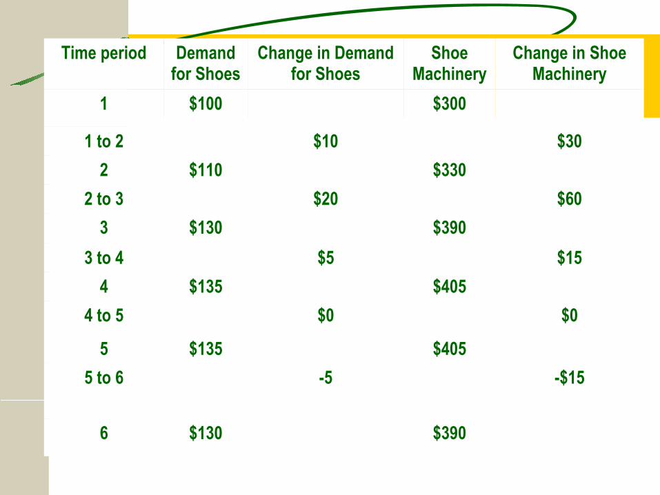
Time period Demand for Shoes

Change in Demand for Shoes

Shoe Machinery

Change in Shoe Machinery

1 $100 $300

1 to 2 $10 $30

2 $110 $330

2 to 3 $20 $60

3 $130 $390

3 to 4 $5 $15

4 $135 $405

4 to 5 $0 $0

5 $135 $405

5 to 6 -5 -$15

6 $130 $390

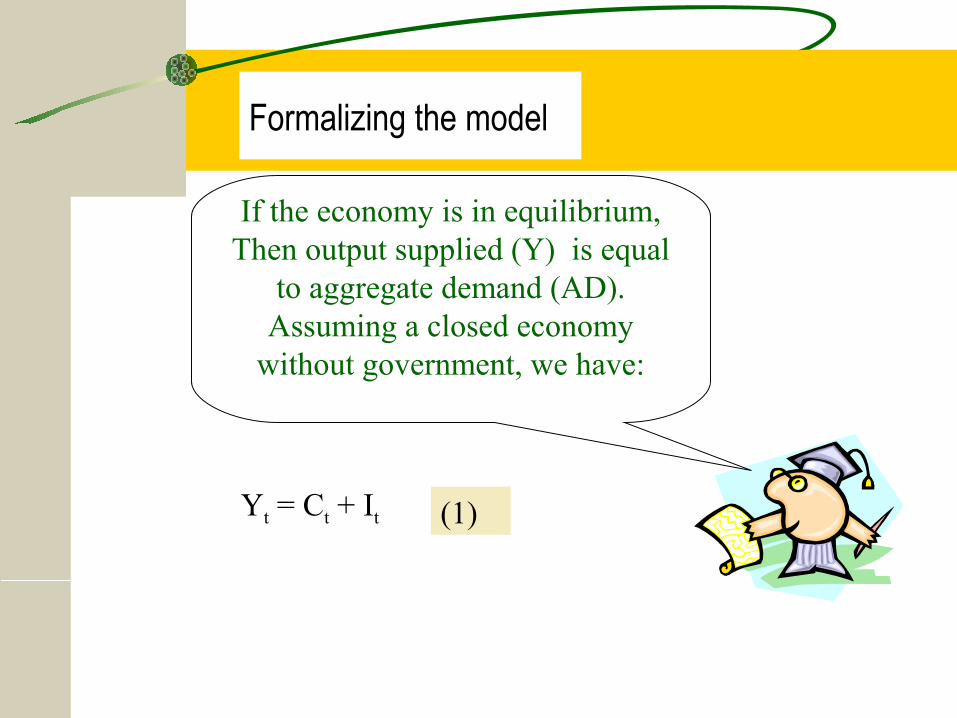
If the economy is in equilibrium,Then output supplied (Y) is equal

to aggregate demand (AD). Assuming a closed economy

without government, we have:

Yt = Ct + It (1)

Formalizing the model

Formalizing the model

•We assume that investment in the current period (It) is equal to some fraction (ν) of change in output in the previous period (or lagged output):

)( 21 −− −= ttt YYI ν (3)

•The consumption function is given by1:

1−+= tt cYCC (2)

1 We assume that C depends on lagged, rather than current, income. Also note that for our simplified economy, Y = YD.

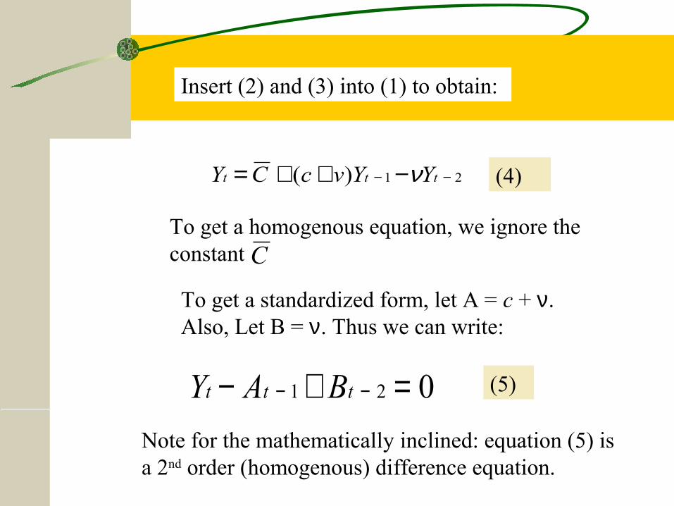
Insert (2) and (3) into (1) to obtain:

21)( −− −++= ttt YYvcCY ν (4)

To get a homogenous equation, we ignore the constant C

To get a standardized form, let A = c + ν. Also, Let B = ν. Thus we can write:

021 =+− −− ttt BAY (5)

Note for the mathematically inclined: equation (5) is a 2nd order (homogenous) difference equation.

It can be shown that:

1. There will be cyclical fluctuations in the time path of national income (Yt) if A2 < 4B.

2. If B = 1 (and presuming that A2 < 4B), then cycles are constant in amplitude.

3. If B < 1 (and presuming that A2 < 4B), then cycles are damped—that is, amplitude is a decreasing function of time.

4. If B > 1 (and presuming that A2 < 4B), then cycles are explosive—that is, amplitude is a increasing function of time.

5. There will be no cyclical fluctuations if A2 > 4B.

Period C Y Net I1 $9962 $1,0003 $996 1000 $44 996 996 05 992 988 -46 985 977 -87 975 965 -118 964 952 -129 953 940 -1310 942 930 -1211 933 923 -1012 927 920 -713 928 925 -314 928 933 515 936 944 816 945 956 1117 957 969 1218 969 982 1319 978 991 1320 987 996 921 992 1000 8

Example of the Multiplier-Accelerator

Assumptions: (1) Y is $996 in period 1 and $1000 in period 2; (2) C = 96 + .9Yt - 1; and (3) ν = 1

Multiplier-Accelerator Model

Data in Billions

Time Period

21191715131197531

Na

tiona

l In

co

me (

Y)

1020

1000

980

960

940

920

900

Assumptions: (1) Y is $996 in period 1 and $1000 in period 2; (2) C = 996 + .9Yt -- 1; and (3) ν = B = 1

Time period

Nat

iona

l Inc

ome

Damped oscillations

B < 1 and A2 > 4B

Time period

Nat

iona

l Inc

ome

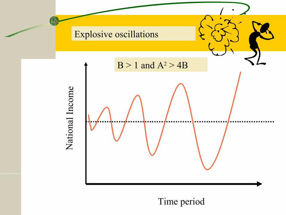
Explosive oscillations

B > 1 and A2 > 4B

Qualifications/limitations

•This model is based on a crude theory of investment. There is no role for “expected profits” or “animal spirits.”

•The time lag between a change in output and a change in (net) investment can be significant—the investment process (planning, finance, procurement, manufacturing, installation, training) is often lengthy.

•J. Hicks pointed out that, for the economy as a whole, there is a limit to disinvestment (negative net investment). At the aggregate level, the limit to capital reduction in a given period is the wear and tear due to depreciation.