Acceleration of the Jacobi iterative method by factors exceeding

100 using scheduled relaxation

Xiang Yang, Rajat Mittal

Department of Mechanical Engineering, Johns Hopkins University, MD, 21218

Abstract

We present a methodology that accelerates the classical Jacobi iterative method by factorsexceeding 100 when applied to the finite-difference approximation of elliptic equations onlarge grids. The method is based on a schedule of over- and under-relaxations that preservesthe essential simplicity of the Jacobi method. Mathematical conditions that maximize theconvergence rate are derived and optimal schemes are identified. The convergence rate pre-dicted from the analysis is validated via numerical experiments. The substantial accelerationof the Jacobi method enabled by the current method has the potential to significantly ac-celerate large-scale simulations in computational mechanics, as well as other arenas whereelliptic equations are prominent.

Keywords: Iterative method, Jacobi method, Elliptic equations

1. Introduction

Elliptic equations appear routinely in computational fluid and solid mechanics as well asheat transfer, electrostatics and wave propagation. Discretization of elliptic partial differen-tial equations using finite-difference or other methods leads to a system of linear algebraicequations of the form Au = b, where u is the variable, b the source term, and A, a bandedmatrix that represents the coupling between the variables. In the context of computationalfluid mechanics, which is of particular interest to us, the Poisson equation for pressure ap-pears in the majority of incompressible Navier-Stokes solvers [1, 2], and is by far, the mostcomputationally intensive component of such simulations. Thus, any effective methods thatcan accelerate the numerical solution of such equations would have a significant impact oncomputational mechanics and numerical methods.

The early history of iterative methods for matrix equations goes back to Jacobi [3] andGauss [4], and the first application of such methods to a finite-difference approximationof an elliptic equation was by Richardson [5]. The method of Richardson, which can beexpressed as un+1 = un − ωn (Au

n − b) , where ‘n’ and ω are the iteration index and therelaxation factor respectively, was a significant advance since it introduced the concept of

Email addresses: xyang44@jhu.edu (Xiang Yang), mittal@jhu.edu (Rajat Mittal)

Preprint submitted to Journal of Computational Physics June 3, 2014

convergence acceleration through successive relaxation. Richardson further noted that ωcould be chosen to successively eliminate individual components of the residual. However,this required knowledge of the full eigenvalue spectrum of A, which was impractical. Giventhis, Richardson’s recipe for choosing ω was to distribute the “nodes”(or zeros) of the ampli-fication factor evenly within the range of eigenvalues of A. This was expected to drive downthe overall amplification factor for the iterative scheme, and the advantage of this approachwas that it required knowledge of only the smallest and largest eigenvalue of A.

Richardson’s method subsequently appeared in the seminal doctoral dissertation of Young[6]. Noting, however, that “... it appears doubtful that a gain of a factor of greater than5 in the rate of convergence can in general be realized unless one is extremely fortunate inthe choice of the values of ω”, Young discarded this method in favour of successive over-relaxation of the so-called Liebmann Method [7], which was essentially the same as theGauss-Seidel method. This seems to signal the end of any attempts to accelerate Jacobi orJacobi-like methods for matrix equations resulting from discrete approximations of ellipticequations.

In this article we describe a new approach for accelerating the convergence of the Ja-cobi iterative method as applied to the finite-difference approximation of elliptic equations.Using this approach, gains in convergence-rate well in excess of a factor of 100 are demon-strated for problems sizes of practical relevance. The increase of processor count in parallelcomputers into the tens of thousands that is becoming possible with multi-core and GPUarchitectures [8], is leading to an ever-increasing premium on parallelizability and scalabilityof numerical algorithms. While sophisticated iterative methods such as multigrid (MG) arehighly efficient on a single processor [9], it is extremely difficult to maintain the convergenceproperties of these methods in large-scale parallel implementations. The domain decomposi-tion approaches associated with parallel implementations negatively impact the smoothingproperties of the iterative solvers used in MG, and also limit the depth of coarsening insuch methods; both of these can significantly deteriorate the convergence properties of MGmethods. In addition to this, the ratio of computation to communication also decreases forthe coarse grid corrections, and this further limits the scalability of these methods. Withinthis context, the iterative method described here, preserves the insensitivity of the Jacobimethod to domain decomposition, while providing significant convergence acceleration.

Another class of methods that is extensively used for solving elliptic equations is conju-gate gradient (CG) [10]. CG methods, however, require effective preconditioners in order toproduce high convergence rates; in this context, the method proposed here could eventuallybe adapted as a preconditioner for CG methods. Thus, the method described here could beused as an alternate to or in conjunction with these methods, and as such, could a have asignificant impact in computational mechanics as well as other fields such as weather andclimate modelling, astrophysics and electrostatics, where elliptic equations are prominent.

Finally, the slow convergence rate of the Jacobi iterative method and the inability toaccelerate this method using relaxation techniques is, at this point, considered textbookmaterial [10, 11, 12]. In most texts, a discussion of the Jacobi method and its slow con-vergence is followed immediately by a discussion of the Gauss-Seidel method as a fasterand more practical method. In this context, the method described here demonstrates that

2

it is in-fact, relatively easy to increase the convergence rate of the Jacobi method by fac-tors exceeding those of the classical Gauss-Seidel method. It is therefore expected that themethod presented here will have a fundamental impact on our view of these methods, andspur further analysis of the acceleration of these basic methods.

2. Jacobi with successive over-relaxation (SOR)

We employ a 2D Laplace equation in a rectangular domain of unit size as our modelproblem: ∂2u/∂x2 + ∂2u/∂y2 = 0. A 2nd-order central-difference discretization on a uniformgrid followed by the application of the Jacobi iterative method with a relaxation parameterω, leads to the following iterative scheme:

un+1i,j = (1− ω)un

i,j +ω

4

(uni,j−1 + un

i,j+1 + uni−1,j + un

i+1,j

)(1)

where n is the index of iteration. von Neumann analysis [11] of the above scheme results inthe following amplification factor:

Gω (κ) = (1− ωκ) with κ (kx, ky) = sin2 (kx∆x/2) + sin2 (ky∆y/2) (2)

where ∆x and ∆y are the grid spacings and kx and ky the wave-numbers in the correspondingdirections. The largest value of κ is given by κmax = 2. The smallest non-zero valueof κ depends on the largest independent sinusoidal wave that the system can admit. ANeumann(N) problem allows waves to be purely one-dimensional, i.e. elementary waves canhave kx = 0 or ky = 0, whereas for Dirichlet(D) problems, one-dimensional waves are, ingeneral, not admissible, and kx, ky must all be non-zero. Therefore the corresponding κmin

are given by:

κNmin = sin2

(π/2

max(Nx, Ny)

); κD

min = sin2

(π/2

Nx

)+ sin2

(π/2

Ny

)(3)

The above expressions are true for a uniform mesh and section 8 describes the extension ofthis approach to non-uniform meshes.

The convergence of the iterative scheme requires |G| < 1 for all wave numbers, and it iseasy to see from Eqn.(2) that over-relaxation of the Jacobi method violates this requirement.Furthermore, for a given grid, κN

min < κDmin; thus Neumann problems have a wider spectrum

and are therefore more challenging than the corresponding Dirichlet problem. We thereforefocus most of our analysis on the Neumann problem. We also note that while the aboveanalysis is for 2D problems, corresponding 1D and 3D problems lead to exactly the sameexpressions for the amplification factors, and similar expressions for κmin, with a pre-factordifferent from unity.

3. Jacobi with over-relaxation: an example

A simple example is presented here in order to motivate the current method. We startby noting that for relaxation factors ≥ 0.5, there is one wave number with an amplification

3

factor equal to zero, and this implies that for a discretized system with N unknowns, itshould be possible to obtain the solution in N iterations by employing a successively relaxediteration with relaxation factors at each iteration chosen to successively eliminate each wave-number component of the error. We explore the above idea further via the following simpleone-dimensional example:

∂2u

∂x2= 0, x ∈ [0, 1], u(0) = 0, u(1) = 0

The above equation is discretized on a five-point equispaced grid. Since the boundary values(u1 and u5) are given, the resulting 3× 3 system that is to be solved is as follows:−2 1 0

1 −2 10 1 −2

u2

u3

u4

=

000

Application of the Jacobi method to this system gives:un+1

2

un+13

un+14

=

0 1/2 01/2 0 1/20 1/2 0

un2

un3

un4

Incorporating successive over-relaxation in to this iteration gives:un+1

2

un+13

un+14

=

(1− ω)I + ω

0 1/2 01/2 0 1/20 1/2 0

un2

un3

un4

We now need to choose a relaxation factor for each iteration such that we can reach theexact solution in three iterations. This condition leads to a cubic equation for ωk

3∏k=1

(1− ωk)I + ωk

0 1/2 01/2 0 1/20 1/2 0

= 0

The roots of this equation can be uniquely determined and they are as follows (in descendingorder of magnitude):

ω1 = 2 +√2, ω2 = 1 and ω3 = 2−

√2

Thus, with the above unique choice of ωs, the exact solution (barring round-off error) can beobtained in 3 iterations starting from an arbitrary initial guess. This idea of eliminating oneparticular wave-number component of the error in each iteration is however not practical,since it is difficult to know a-priori, the correct relaxation factor for each iteration. Besides,even if appropriate ωk could be determined, the error-component for any wave number that iseliminated in a given iteration could reappear due to roundoff error and possibly be amplifiedin subsequent iterations since over-relaxation does generate amplification factors that exceed

4

unity for some wave numbers. The above analysis is nevertheless insightful: considering thefact that the ωk above are uniquely determined, it necessarily implies that constrained tounder-relaxation (note that ω1 > 1), it is not possible to obtain the solution in ≤ N steps.In fact, it is interesting to note that without any over- or under-relaxation, the error wouldbe reduced by a factor of only (1/2)3 = 1/8 (approximately one order-of-magnitude) in threeiterations. Thus, over-relaxation does not necessarily produce divergence in the iteration; onthe contrary, when combined with under-relaxation, it can help accelerate the convergenceof JM.

4. Scheduled Relaxation Jacobi (SRJ) Schemes

The method described here (termed “SRJ” for Scheduled Relaxation Jacobi) consists ofan iteration cycle that further consists of a fixed number (denoted by M) of SOR Jacobiiterations with a prescribed relaxation factor scheduled for each iteration in the cycle. TheM -iteration cycle is then repeated until convergence. This approach is inspired by the obser-vation that over relaxation of Jacobi damps the low wavenumber residual more effectively,but amplifies high wavenumber error. Conversely, under-relaxation with the Jacobi methoddamps the high wave number error efficiently, but is quite ineffective for reducing the lowwavenumber error. The method we present here, attempts to combine under- and over-relaxations to achieve better overall convergence. Our goal is to provide a set of schemesthat practitioners can simply select from and use, without going through any of the analysisperformed in this paper.

4.1. Nomenclature

Each SRJ scheme is characterized by the number of ‘levels’, which corresponds to thenumber of distinct values of ω used in the iteration cycle. We denote this parameter byP and the P distinct values of ω used in the cycle are represented by the vector Ω =ω1, ω2, . . . , ωP. For the uniqueness of Ω, we sequence those P distinct values of relaxation

factors in descending order, i.e. ω1 > ω2 > . . . > ωP . Second, we define Q = q1, q2, . . . , qP,where qi is the number of times the value ωi is repeated in an SRJ cycle. We also defineβ = β1, β2, ..., βP where βi = qi/M , is the fraction of the iterations counts of ωi in oneSRJ iteration cycle. Due to the linearity of Eq.(1), the sequencing of the ωs within a cycledoes not affect the analysis of convergence. In practice, however, due to the roundoff andarithmetic overflow associated with digital computers, appropriate sequencing of the ω ’smight be require; this issue that will be discussed later in the paper. P , Ω and Q (or β)therefore uniquely define an SRJ scheme. It is noted that Richardson proposed to use adifferent relaxation factor for each iteration in a cycle; that idea may be viewed as a specialcase of the SRJ scheme with P = M and qi ≡ 1.

4.2. Amplification Factor

If one iteration of SOR-Jacobi attenuates the wave with a vector wavenumber (kx, ky) bythe factor of G (κ (kx, ky)), then the amplification factor for the one full SRJ cycle (defined

5

as G(κ; Ω, Q) ) consisting of M iterations is given by

G(κ; Ω, Q) =P∏i=1

(Gωi(κ))qi (4)

where Gωiraised to the power of qi is simply because the relaxation factor ωi is repeated qi

times in one cycle. Following this, we define the per-iteration amplification factor for thiscycle as the geometric mean of the modulus of the cycle amplification factor G(κ; Ω, Q), i.e.

Γ (κ (kx.ky)) =∣∣∣G(κ; Ω, Q)

∣∣∣ 1M

=P∏i=1

|1− ωiκ|βi (5)

5. Two-Level (P=2) Schemes

We begin our analysis with the two-level (P = 2) SRJ scheme, for which Ω = ω1, ω2and β = β1, β2. The per-iteration amplification factor for this 2-level scheme can beexpressed as

Γ (κ) = [|1− ω1κ|q1 |1− ω2κ|q2 ]1M = |1− ω2κ/α|β |1− ω2κ|1−β (6)

where α = ω2/ω1, and β1, which is equal to (1− β2), is replaced by β for notational simplicity.The three variables α, ω2, β control the convergence of any P = 2 SRJ. Since Γ(κ) < 1must be satisfied, we cannot have both ω1, ω2 larger than 1, and because we order relaxationfactors such that ω1 > ω2, ω2 is necessarily ≤ 1. Moreover, by definition, α and β also liewithin [0, 1].

The maximum magnitude of Γ in the closed interval [κmin, κmax], denoted as Γmax, de-termines the asymptotic convergence of an iterative scheme[11]. Following convention, theconvergence rate of a given iterative scheme can be measured by the number of iterationsrequired to reduce the residual by an order of magnitude. This number, denoted here byN0.1, is given by the following formula: N0.1 = ln(0.1)/ln (Γmax). Finally, for each iterativemethod, we also define a convergence performance index ρ as the ratio of N0.1 for the classicJacobi method to N0.1 for the iterative method under consideration.

5.1. Optimal P=2 schemes

The asymptotic convergence of the iterative scheme can be maximized by minimizingthe maximum value of Γmax for any given grid size N . A simple analysis of Eq.(6) showsthat Γmax for P = 2 schemes could be located at one of the following locations:

κ1 = κmin; κ2 = (α+ β − αβ) /ω2 and κ3 = κmax ≡ 2 (7)

where κ2 is the coordinate of the internal extremum for (6). This is determined by firstnoting that the local extremum of log Γ (κ) coincides with that of Γ (κ), and then solving

the equation d log Γ(κ)dκ

= 0 for the form of Γ given in Eqn.(6)

6

Among Γ (κ1), Γ (κ2), Γ (κ3), the value of Γ(κ1) is strongly constrained by the conditionΓ(0) ≡ 1 and therefore, the minimization of Γ(κ1) has to be the driving factor in theconvergence maximization. Thus, Γ(κ1) should be the global maximum and we thereforerequire:

Γ(κ2) ≤ Γ(κmin), Γ(κ3) ≤ Γ(κmin) (8)

However, Γ, is a function of three independent variables: ω2, α and β, and minimizationof Γ(κmin) under the constraints of (8) is not straightforward. The mathematical problemcan, however, be simplified by first we noting that Γ(κmin), is a monotonically decreasingfunction of (ω2κmin) near ω2κmin = 0. Since we have

d log (Γ)

d(ω2κ)=

1

Γ

dΓ

dω2κ(9)

the sign of d log (Γ)/d(ω2κ) is the same as that of dΓ

/dω2κ. Hence to check the monotonicity

near 0, we only need to check the sign of d log (Γ)/d(ω2κ) at ω2κmin = 0. This is given by

d log (Γ)

d(ω2κ)

∣∣∣∣ω2κmin=0

= −1 + β − β

α< 0 (10)

Since κminω2 is very close to 0, it is safe to argue that with other variable unchanged, asmaller ω2κmin could result in a smaller Γ (κmin). In addition, we also have

Γ(κ2) =

∣∣∣∣βα(1− α)

∣∣∣∣β |(1− α)(1− β)|1−β (11)

which indicates that Γ(κ2) is independent of ω2. Therefore, if the first condition in (8)is satisfied strictly with an inequality, it is possible to increase ω2 to reduce Γ(κmin), themaximum of Γ, without violating the first condition in (8). Hence to minimize Γ(κmin), thefirst condition in (8) should be satisfied with an equality. Employing the same argument,it is easy to see that the second condition in (8) should also be satisfied with an equality.Condition (8) is therefore reduced to:

Γ(κ2) = Γ(κmax) = Γ(κmin) (12)

Maximization of convergence rate of the P=2 SRJ scheme is therefore equivalent to mini-mizing Γmax under the two conditions in (12). Given that κmin is essentially a surrogate forthe grid size (see Eq.(3)) the above provides sufficient conditions to uniquely determine aset of α, β, ω2 values that maximize the asymptotic convergence rate for a given grid.

The equations that result from the above procedure are shown in Appendix A where thethree primary unknowns are augmented by two ancillary variables ∂α/∂β and ∂ω2/∂β. Theaddition of these two variables facilitates the implementation of the above procedure. Wenote that these equations are highly non-linear and coupled in a complex way.

7

10−2

10−1

100

0

0.2

0.4

0.6

0.8

1

Γ

κ

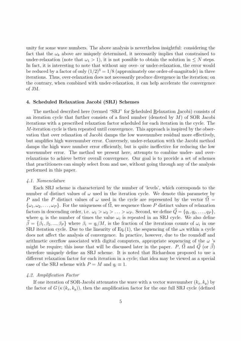
Figure 1: Amplification factor curves for selected optimal P=2 SRJ schemes. Comparison between Jacobimethod (· − ·), optimal M = 2 (−) and optimal P = 2 (M > 2) (−−) scheme for N=16.

5.2. M=2 schemes

A closed-form solution of the above equations is obtained only for schemes with M =2 (β = 0.5) and is as follows:

α =(−b−

√b2 − 4

)/2 and ω2 = (α + 1) / (2 + κmin)

where b =2κmin − 6 (2 + κmin)

2

κmin + (2 + κmin)2

(13)

The above expressions asymptote for κmin ≪ 2 which, based on (3), occurs at fairly smallvalues of N . The asymptotic values of ω1 and ω2 are 3.414213 and 0.585786 respectively,and the asymptotic value of ρ for this scheme is precisely equal to 2.0. Numerical testsof this for a 2D Neumann problem and a random initial guess indicate a ρ value of 1.99which confirms the predicted convergence. Thus, even the two-step SRJ scheme, which isthe simplest possible extension of the classic Jacobi method, doubles the rate of convergence,a rate that matches that of the classical point-iterative Gauss-Seidel method.

5.3. M > 2 schemes

For P = 2;M > 2 schemes, we have employed a MATLAB based numerical procedureto solve the equation-set shown in Appendix A, and Table 1 shows the optimal parametersobtained from this process for a 2D Neumann problem on a uniform N × N grid. Fig.1shows plots of the amplification factor for optimal M = 2 and M > 2 scheme for N = 16along with the amplification factor for the classic Jacobi method. It is noted that while theJacobi method has one node, the P = 2 SRJ schemes have two nodes. Furthermore, theplots clearly show the effect of relaxing the M = 2 constraint for two-level schemes: the firstnode in Γ is pushed closer to κ = 0 thereby reducing Γ (κmin).

8

Table 1: Parameters and performance of optimized two-level (P=2) SRJ schemes for a range of grid sizesN . ρtest is the value obtained from numerical tests for the Neumann problem and N excludes the boundarypoints.

N SRJ Scheme N0.1 ρ (q1, q2) ρtest

16Ω = 32.60, 0.8630

72 3.31 (1,15) 3.41β = 0.064291, 0.93570

32Ω = 81.22, 0.9178

251 3.81 (1,30) 4.00β = 0.032335, 0.96766

64Ω = 190.2, 0.9532

923 4.14 (1,63) 4.51β = 0.015846, 0.98415

128Ω = 425.8, 0.9742

3521 4.34 (1,130) 4.34β = 0.0076647, 0.99233

256Ω = 877.8, 0.98555

13743 4.45 (1,257) 4.50β = 0.0036873, 0.996312

512Ω = 1972, 0.99267

54119 4.52 (1,564) 4.69β = 0.0017730, 0.998227

1024Ω = 4153, 0.99615

214873 4.55 (1,1172) 5.35β = 0.00085251, 0.9991474

Table 1 shows that ω1 for these optimal schemes is significantly larger than unity for allN , and it increases rapidly with this parameter. This is expected since κmin decreases withincreasing N and the scheme attempts to move the first node closer to κ = 0 in order toreduce the amplification factor at κmin. On the other hand, ω2 is very close to unity andbecomes increasingly so with N . It is also noted that β1 is significantly smaller than β2

(which, is equal to (1− β1)) for all cases and becomes smaller with increasing N . Thus, thescheme compensates for an increasing over-relaxation parameter ω1 primarily by increasingβ2 relative to β1. Furthermore, N0.1 is found to increase with N and this rate of increasewith N will be addressed later in the paper.

The ρ for the optimal P = 2 schemes is found to range from 3.31 to 5.35 for the valuesof N studied here. Thus, even within the constraint of two-levels, loosening of the M = 2constraint results in a significant additional increase in the convergence rate. Note also thatthese optimal two-level SRJ schemes are now roughly twice faster than GSM. Furthermore,this speed-up is similar to the maximum gain possible with the method of Richardson [6].

For numerical validation of the above schemes, we choose q1 ≡ 1 and q2 = ⌈β2

β1⌉. The use

of the ceiling function increases the under-relaxation very slightly over the optimal value andshould enhance numerical stability. This value of Q is also shown in Table 1 and we notethat q2 increases from 15 for N = 16 to 1172 for N = 1024. Thus, in all of these schemes,one over-relaxation step is followed by a fairly large number of under-relaxations. We haveimplemented the schemes with (q1, q2) given in the table for a 2D Laplace equation on auniform, isotropic grid with a cell-centered arrangement. Results for the Neumann problemonly are reported here since the Dirichlet problems exhibit similar trends.

The initial guess in these tests corresponds to a random value in the range [0, 1] at each

9

grid point and Table 1 shows that the numerical tests exhibit a convergence performanceindex (ρtest) that is equal to or slightly higher than the predicted value. It is noted thatthe condition of optimality equalizes the multiple extrema in Γ. However, due to the finite-precision mathematics employed in the optimization process as well as the round-off errorsinherent in the numerical validation, there is a small but finite imbalance between the variousvalues of Γmax and this can make the convergence behaviour somewhat sensitive to the initialguess. Numerical tests with other initial guesses such as a Dirac δ-function confirm thissensitivity. However, for every initial guess that has been tried, the asymptotic convergencerates for the optimal SRJ schemes either equal or slightly exceed the corresponding predictionfrom the mathematical analysis have been observed.

5.4. Sensitivity of optimal SRJ schemes

For practical implementation of the SRJ schemes, it is desired that N0.1 not increasesignificantly if parameters that are close, but not exactly equal to the optimal set, areemployed. This issues is addressed in the current section.

We first prove that if a set of parameters that is optimized for a given system size (i.e.given N) is employed to solve a larger system, the acceleration index ρ will not decrease be-low that of the smaller system. For this, we note that for sufficiently large N , Γ(κmin) can beapproximated via a Taylor series as Γ(κmin) ≈ Γ(0) + κmin∂Γ/∂κ|κ=0 = 1 + κmin∂Γ/∂κ|κ=0.Assuming further that the scheme under consideration is optimized using the process de-scribed in the previous sections, Γmax = Γ (κmin), and the convergence performance indexcan then be estimated as:

ρ ≈ln(1 + κmin

∂ΓSRJ

∂κ

∣∣κ=0

)ln(1 + κmin

∂ΓJM

∂κ

∣∣κ=0

) ≈∂ΓSRJ

∂κ

∣∣κ=0

∂ΓJM

∂κ

∣∣κ=0

=P∑i=1

ωiβi (14)

It is noted that the above expression is independent of κmin and therefore, for a fixed set ofparameters (i.e. Ω and β), ρ is independent of system size N , as long as Γmax = Γ(κmin).Since Γ (κmin) has a negative slope at κ = 0, and κmin is smaller for a largerN , Γmax = Γ(κmin)will be true if a set of parameters that is optimized for a smaller system is applied to a largersystem. The converse, i.e. using a set of parameters that is optimized for a large system toa smaller system, is however not recommended; in that case Γ(κmin) decreases and becauseall the interior extrema have to be balanced with Γ (κmin), Γ(κmin) is not guaranteed to beΓmax. We also note that in this analysis, the dimension of the problem does not enter in toconsideration and therefore, parameters optimized for a 2D problem can be safely used forcorresponding 3D problem. This is demonstrated later in the paper.

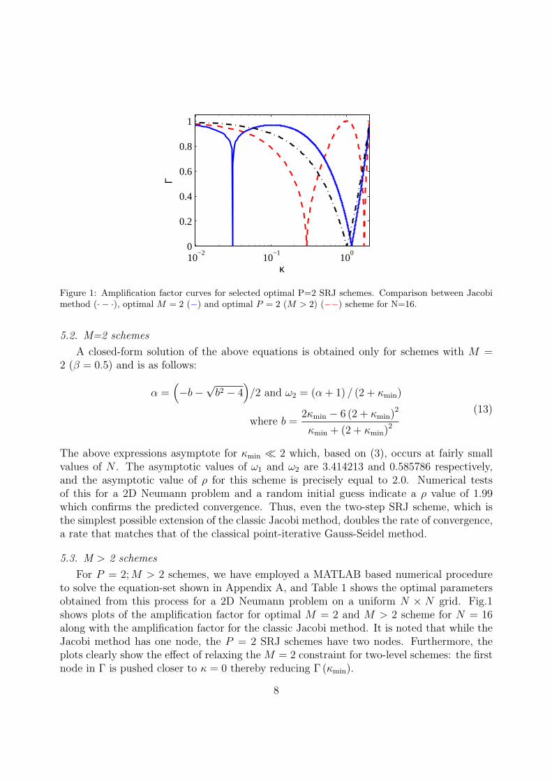
We further explore the sensitivity of the convergence rate to scheme parameters via Fig.2, which shows the effect of cycle size M on ρ. Each point on the curve corresponds to ascheme optimized for a given M for the 2D Neumann problem. The maximum in ρ observedin the various curves (and marked by circles) correspond to the global optima that areidentified in Table 1. The plot indicates that for small values of N , the maximum in ρ issharp, indicating a relatively high sensitivity to the scheme parameters. However, for largervalues of N , while the performance deteriorates rapidly as M is reduced from the optimal

10

0 100 200 300 400 5001.5

2

2.5

3

3.5

4

4.5

M

ρ

Figure 2: Convergence performance index ρ versus M for P = 2 schemes that are optimized for a givenvalue of M . N = 16 (· − ·); N = 32(· · ·); N = 64(−−); and N = 128( −). Circles identify the globallyoptimal scheme for each N .

value, the effect on performance is relatively weak as M is increased beyond the optimalvalue. This insensitivity is particularly pronounced for the highest values of N in the plot,which exhibits a very broad maxima. This is particularly useful since problems of practicalrelevance in computational mechanics are expected to have large grid sizes.

While small changes that are introduced to enhance the stability of the given schemeare not expected to deteriorate the convergence significantly, caution should be exercisedin making ad-hoc modifications in some parameters. For instance, based on Table 1, theremight be a temptation to simply put ω2 equal to 1 for large N . However, this would eliminatethe under-relaxation that is necessary to balance out the over-relaxation, and would leadto divergence. Similarly, starting from an optimal set of parameters, the over-relaxationfactor ω1 should only be decreased since increasing it would lead to instability. Thus, it isadvisable to round down the value of the over-relaxation parameters determined from theoptimization process.

6. Multilevel (P > 2) Schemes

In this section, we examine the convergence gains possible with multilevel (P > 2)schemes. The general procedure for optimizing multilevel schemes is summarised in Ap-pendix B and the ideas behind the equations are briefly described here. The constraint thatall local extrema are equalized with Γmax is still enforced. The parameters βi, i = 1, 2, ..., P−1are considered to be truly free parameters, with ωi depending on them. The optimizationis then with respect to βi, i = 1, 2, ..., P − 1, and this procedure results in intermediateunknowns like ∂ωi/∂βj. We note that βP is not a free parameter because of the constraint∑P

i=1 βi = 1. The size of this complex non-linear system grows proportional to P 2 and thissystem of equations can therefore only be solved numerically. Furthermore, large values of

11

10−3

10−2

10−1

100

0

0.2

0.4

0.6

0.8

1

κ

Γ

Figure 3: Comparison between optimal P = 3 scheme for N = 16 (· − ·)and N = 32 (−). Γ(κmin) for eachcase is denoted by . For the curve of N = 16, κmin = 0.0096, κ1 = 0.0351, κ2 = 0.4282 and Γmax = 0.946,while for the N = 32 curve, κmin = 0.0024, κ1 = 0.0125, κ2 = 0.2689 and Γmax = 0.981.

N (i.e. small values of κmin) combine with large values of P to increase the stiffness of thesystem of equations. Thus, optimal schemes presented in the paper are currently limited toP = 5.

6.1. Optimal multilevel schemes

Table 2, 3 and 4 shows the optimal values that have been obtained from the numericaloptimization process for P = 3, 4 and 5 SRJ schemes, respectively. The trends in the tableare similar to those observed for the P = 2 schemes. First, except for one stage of under-relaxation, all other stages in the sequence are over-relaxations, and the over-relaxationfactors increase monotonically with N . Fig.3 shows plots of the amplification factor foroptimal P = 3 schemes for N = 16 and 32. The plots clearly show that the optimizationprocess moves the first node in Γ closer to the origin as N increases.

For one case (N = 64) in each table, we have also included results for a three-dimensionalcase. As predicted from the analysis in Sec. 5.4, the increase in the dimensionality of theproblem from one to three does not affect the performance of the scheme. Thus, schemesidentified as optimal from the 1D analysis can be used safely in the corresponding 2D and3D problems.

The tables therefore clearly demonstrate significant increases in convergence accelerationwith increasing P . For instance, comparing the case of N = 512 for which we have derivedoptimized P = 2, 3, 4 and 5 schemes, we note that ρ increases from about 5 for P = 2to about 68 for P = 5. Higher gains in convergence will likely be obtained for larger Palthough this remains to be formally demonstrated. Nevertheless, it is clear that multilevelSRJ schemes offer significantly higher convergence rates.

12

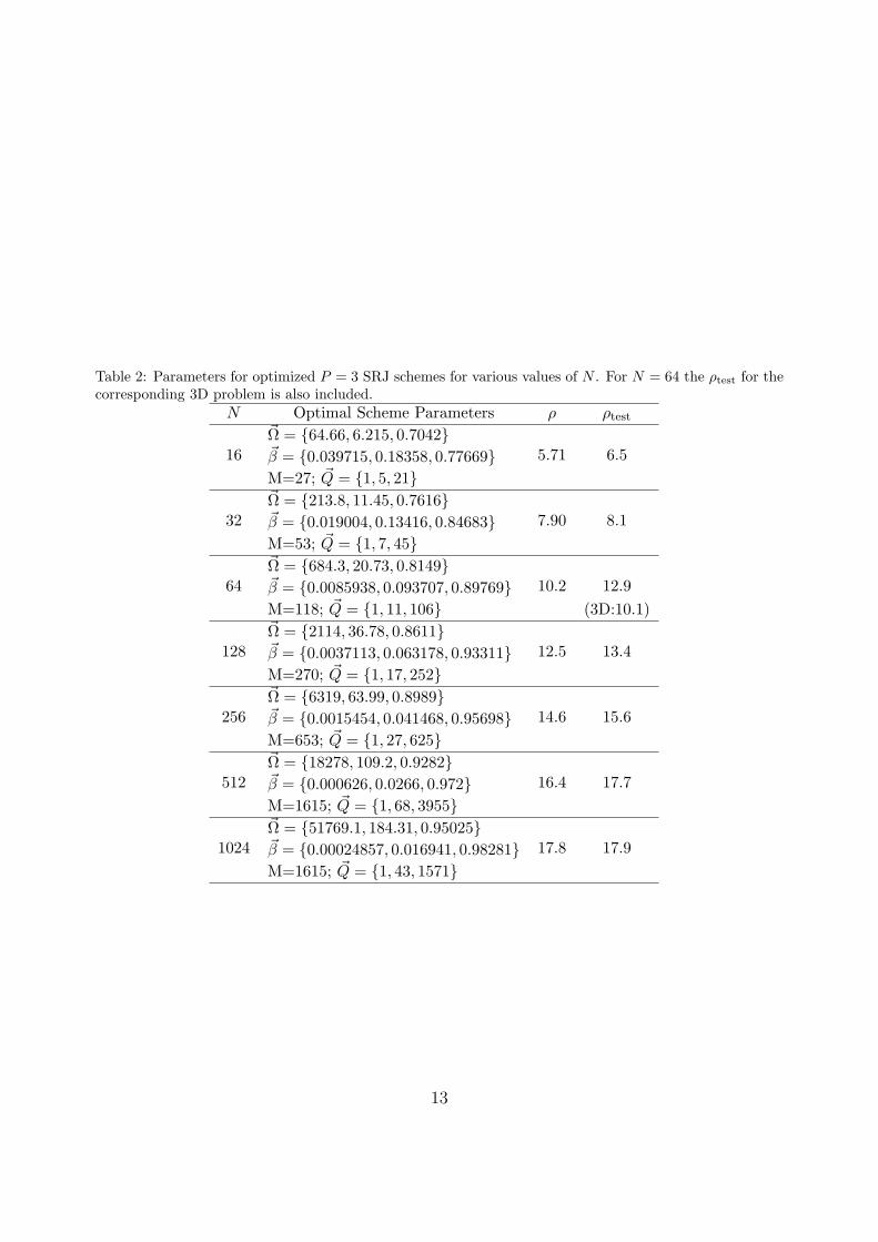
Table 2: Parameters for optimized P = 3 SRJ schemes for various values of N . For N = 64 the ρtest for thecorresponding 3D problem is also included.

N Optimal Scheme Parameters ρ ρtest

16Ω = 64.66, 6.215, 0.7042

5.71 6.5β = 0.039715, 0.18358, 0.77669M=27; Q = 1, 5, 21

32Ω = 213.8, 11.45, 0.7616

7.90 8.1β = 0.019004, 0.13416, 0.84683M=53; Q = 1, 7, 45

64Ω = 684.3, 20.73, 0.8149

10.2 12.9β = 0.0085938, 0.093707, 0.89769M=118; Q = 1, 11, 106 (3D:10.1)

128Ω = 2114, 36.78, 0.8611

12.5 13.4β = 0.0037113, 0.063178, 0.93311M=270; Q = 1, 17, 252

256Ω = 6319, 63.99, 0.8989

14.6 15.6β = 0.0015454, 0.041468, 0.95698M=653; Q = 1, 27, 625

512Ω = 18278, 109.2, 0.9282

16.4 17.7β = 0.000626, 0.0266, 0.972M=1615; Q = 1, 68, 3955

1024Ω = 51769.1, 184.31, 0.95025

17.8 17.9β = 0.00024857, 0.016941, 0.98281M=1615; Q = 1, 43, 1571

13

Table 3: Parameters for optimized P = 4 SRJ schemes for various values of N . For N = 64 the ρtest for thecorresponding 3D problem is also included.

N Optimal Scheme Parameters ρ ρtestΩ = 80.154, 17.217, 2.6201, 0.62230

7.40 7.716 β = 0.031495, 0.082068, 0.25554, 0.63089M=31; Q = 1, 2, 8, 20Ω = 289.46, 40.791, 4.0877, 0.66277

11.3 11.832 β = 0.015521, 0.053883, 0.22041, 0.71018M=64; Q = 1, 3, 14, 46Ω = 1029.4, 95.007, 6.3913, 0.70513

16.6 15.264 β = 0.0072290, 0.033832, 0.18222, 0.77671M=146; Q = 1, 5, 26, 114 (3D:16.3)

Ω = 3596.4, 217.80, 9.9666, 0.7475523.1 24.7128 β = 0.0032024, 0.020392, 0.145608, 0.83079

M=343; Q = 1, 7, 50, 285Ω = 12329, 492.05, 15.444, 0.78831

30.8 34.2256 β = 0.0013564, 0.011845, 0.11316, 0.87362M=760; Q = 1, 9, 86, 664Ω = 41459, 1096.3, 23.730, 0.82597

39.0 44.2512 β = 0.00055213, 0.0066578, 0.085990, 0.90680M=1818; Q = 1, 12, 155, 1650

14

Table 4: Parameters for optimized P = 5 SRJ schemes for various values of N . For N = 64 the ρtest for thecorresponding 3D problem is also included.

N Optimal Scheme Parameters ρ ρtestΩ = 88.190, 30.122, 6.8843, 1.6008, 0.58003

8.5 8.816 β = 0.026563, 0.050779, 0.12002, 0.28137, 0.52126M=43; Q = 1, 2, 5, 12, 23Ω = 330.57, 82.172, 13.441, 2.2402, 0.60810

14.0 13.232 β = 0.013467, 0.031695, 0.092173, 0.26580, 0.59686M=76; Q = 1, 2, 7, 20, 46Ω = 1228.8, 220.14, 26.168, 3.1668, 0.63890

22.0 20.464 β = 0.0064862, 0.019035, 0.068043, 0.24139, 0.66504M=158; Q = 1, 3, 10, 38, 106 (3D:20.2)

Ω = 4522.0, 580.86, 50.729, 4.5018, 0.6716133.2 31.0128 β = 0.0029825, 0.011020, 0.048530, 0.21238, 0.72508

M=343; Q = 1, 3, 16, 73, 250Ω = 16459, 1513.4, 97.832, 6.4111, 0.70531

48.3 43.1256 β = 0.0013142, 0.0061593, 0.033568, 0.18206, 0.77689M=778; Q = 1, 4, 26, 142, 605Ω = 59226, 3900.56, 187.53, 9.1194, 0.73905

67.7 59.9512 β = 0.00055665, 0.0033286, 0.022588, 0.15273, 0.82079M=1824; Q = 1, 6, 40, 277, 1500

15

103

104

105

106

102

103

104

105

106

N2

N(0

.1)

Figure 4: Effect of grid sizeN on asymptotic convergence rate of various optimized SRJ schemes (P = 2 : ();P = 3 : (), P = 4 : (+) and P = 5 : (×)). The slopes for the best-fit lines for P =2, 3 and 4 schemes are0.97, 0.88, 0.81 and 0.71 respectively. The topmost line corresponds to the classical Jacobi method. Theisolated symbols in the plot identify the SRJ schemes described in Table 5 ( a: (); d:()).

6.2. Scaling of convergence acceleration with grid size

Interesting trends emerge with respect to the effect of N on convergence acceleration. InFig. 4 we compare N0.1 for various grids for the entire set of optimal SRJ schemes that havebeen identified so far and in the later sections. For the classical Jacobi method, N0.1 scaleslinearly with the total number of grid points N2 and this is indeed borne out in our tests.On the other hand, optimal SRJ schemes seem to provide a slower than linear increase inN0.1 with total grid size. The slopes estimated for the lines in Fig. 4 are 0.97, 0.88, 0.81 and0.71 for P=2, 3, 4 and 5 respectively. Thus, the advantage of SRJ schemes over the classicalJacobi is not just through a fixed multiplicative factor in the convergence rate (as is thecase for Gauss-Seidel method that has a constant factor of two) but through a factor thatincreases with grid size. This is highly desirable, since large grid simulations on massivelyparallel computers, are precisely where this method would be most appropriate.

6.3. Trends in cycle size (M)

The cycle size M of optimal SRJ schemes is also of interest, since large cycle sizes wouldbe unattractive from a practical point-of-view. The cycle size M is plotted against N for allP in Fig.5(a) and we find that cycle size grows nearly linearly with N for all values of P .This is not unexpected since increasing N increases the range of wavenumbers and additionaliterations are needed in a given cycle to damp the error at each of these wavenumbers.

Figure 5(b) shows the cycle size M plotted against P for all N and we note that whilefor each N , the cycle-size increases with P , it rapidly approaches an asymptotic value. Thiscombined with the trend shown in Fig. 4 implies that higher convergence rates obtained byincreasing P do not require substantial additional increase in cycle-size.

16

101

102

103

101

102

103

104

N

M

(a)

P=2

P=3

P=4

P=5

2 3 4 50

500

1000

1500

2000

P

M

(b)

N=16N=32N=64N=128N=256N=512

Figure 5: Variation of cycle size M for various multilevel schemes: (a) M versus N for various P ; (b) Mversus P for various N .

6.4. Relaxation Schedule

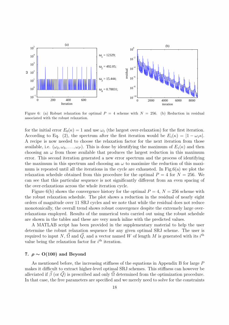
The optimal multilevel schemes identified above have been subjected to numerical vali-dation and in this process, the importance of appropriate scheduling of the iterations duringthe SRJ cycles becomes apparent. We have previously mentioned that the schedule of re-laxation factors does not effect the mathematical analysis of any SRJ scheme. However, inpractice, due to roundoff errors and the arithmetic overflow associated with digital com-puters, appropriate scheduling of the ω ’s during a SRJ cycle might be required to ensurenumerical convergence of the SRJ scheme.

To understand this issue, we note first that for any single iteration that employs anover-relaxation, |G|max = |1− ωκmax| ≡ 2ω − 1. Now consider, for example, the optimalscheme for P = 4 and N = 256 in Table 3 that consists of 760 iterations, of which, 86iterations have a relaxation factor of 15.444. If all of these 86 iterations are carried outin succession, any initial error at κ = 2 would get amplified by a factor of (29.888)86,which would lead to overflow even if the initial error at this wavenumber was machine-zero.Therefore, the appropriate approach to avoid overflow in these schemes is to appropriatelydistribute the relatively few over-relaxation in between multiple under-relaxation. In thisway, any intermediate growth in the high wavenumber residual due to over-relaxation canbe damped appropriately by the under-relaxations.

Our numerical experiments indicate that in most cases an even distribution of the over-relaxations over the entire cycle is sufficient to avoid overflow. Thus for instance, in theparticular case of the optimal scheme for P = 4, N = 256 in Table 3 for which M = 760,Ω = 12329, 492.05, 15.444, 0.78831 and Q = 1, 9, 86, 664, the first iteration would bethe over-relaxation with ω1 = 12329. The 9 iterations with ω2 = 492.05 would be spaced760/9 ≈ 84 iterations apart and the 86 iterations with ω3 = 15.444 would be spaced 760/86 ≈8 iterations apart. All of the intervening iterations would be with the 664 under-relaxationswith ω4 = 0.78831.

In addition to the simple rule for scheduling the iterations provided above, a more formalprocedure is also available to generate a robust schedule that guarantees avoidance of over-flow. This robust schedule is determined as follows: we assume a constant unit spectrum

17

0 200 400 60010

−1

100

101

102

103

104

105

Iteration

ω

ω1 = 12329;

ω2 = 492.05;

ω3 = 15.444;

ω4 = 0.78831;

(a)

0 2000 4000 6000 800010

−10

10−8

10−6

10−4

10−2

100

iteration

resi

dual

(b)

Figure 6: (a) Robust relaxation for optimal P = 4 scheme with N = 256. (b) Reduction in residualassociated with the robust relaxation.

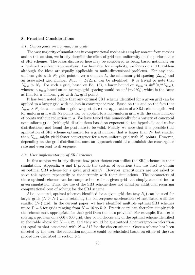
for the initial error E0(κ) = 1 and use ω1 (the largest over-relaxation) for the first iteration.According to Eq. (2), the spectrum after the first iteration would be E1(κ) = |1− ω1κ|.A recipe is now needed to choose the relaxation factor for the next iteration from thoseavailable, i.e. (ω2, ω3, . . . , ωP ). This is done by identifying the maximum of E1(κ) and thenchoosing an ω from those available that produces the largest reduction in this maximumerror. This second iteration generated a new error spectrum and the process of identifyingthe maximum in this spectrum and choosing an ω to maximize the reduction of this maxi-mum is repeated until all the iterations in the cycle are exhausted. In Fig.6(a) we plot therelaxation schedule obtained from this procedure for the optimal P = 4 for N = 256. Wecan see that this particular sequence is not significantly different from an even spacing ofthe over-relaxations across the whole iteration cycle.

Figure 6(b) shows the convergence history for the optimal P = 4, N = 256 scheme withthe robust relaxation schedule. The plot shows a reduction in the residual of nearly eightorders of magnitude over 11 SRJ cycles and we note that while the residual does not reducemonotonically, the overall trend shows robust convergence despite the extremely large over-relaxations employed. Results of the numerical tests carried out using the robust scheduleare shown in the tables and these are very much inline with the predicted values.

A MATLAB script has been provided in the supplementary material to help the userdetermine the robust relaxation sequence for any given optimal SRJ scheme. The user isrequired to input N , Ω and Q, and a vector named W of length M is generated with its ith

value being the relaxation factor for ith iteration.

7. ρ ∼ O(100) and Beyond

As mentioned before, the increasing stiffness of the equations in Appendix B for large Pmakes it difficult to extract higher-level optimal SRJ schemes. This stiffness can however bealleviated if β (or Q) is prescribed and only Ω determined from the optimization procedure.In that case, the free parameters are specified and we merely need to solve for the constraints

18

Table 5: SRJ schemes for some selected N that can accelerate JM by two orders of magnitude. The resultsare for 2D Laplace(ρL) and Poisson(ρP ) equation with Neumann boundary conditions.

index N SRJ Scheme ρ ρL ρP

a 512Ω = 91299, 25979, 3862.1, 549.90, 80.217, 11.992, 1.9595, 0.59145

148 147 151Q = 1, 3, 9, 27, 81, 243, 729, 1337

b 512Ω = 83242, 14099, 1334.1, 126.45, 12.193, 0.79246

90 92 91Q = 1, 4, 16, 64, 256, 2504

b 1024Ω = 178919, 8024.1, 349.03, 15.9047, 0.799909

90 95 97Q = 1, 7, 49, 343, 3087

d 1024Ω = 300015, 47617, 4738.4, 428.51, 39.410, 3.9103, 0.65823

190 199 197Q = 1, 3, 13, 55, 227, 913, 2852

that equalize all the interior extremums to Γmax, and with no intermediate unknowns like∂ωi/∂βj. The parameter set obtained from this procedure will not correspond to the globaloptimum for the given N and P , but could still provide significant convergence acceleration.The goal here is to demonstrate convergence rates for grid sizes of practical interest that aretwo orders of magnitude better than the Jacobi method.

Our preceding analysis suggests that ρ ∼ O(100) would likely necessitate going to higherthan 4-level schemes, and we have therefore focused our search on P ≥ 5 schemes. Taking acue from the observed trends for P ≤ 4 SRJ schemes, we select a rapidly increasing sequencefor βi. In the absence of any other available rule, we choose qi = Ri for i = 1 to P −1, whereR is an integer, and qP was chosen to be significantly larger than (q1+q2+ . . .+qP−1). Table5 shows four selected schemes for values of N being 512 or 1024. We note that P rangesfrom 5 to 8 for these schemes and ρ ranges from 90 to 190. Following this, we execute ourMATLAB algorithm to determine Ω that maximizes the convergence for the given choice ofQ. The fourth scheme in the table was obtained serendipitously during our analysis and isnoted here since it provides the highest (190-fold) convergence acceleration found so far.

The convergence performance predicted from the analysis is tested numerically by em-ploying a robust relaxation schedule as described in section 6.4. The numerical validationdoes indeed bear out the prediction from the analysis and the results presented in this sec-tion therefore indicate that it is relatively easy to construct SRJ schemes that provide a twoorders-of-magnitude increase in convergence rate over the Jacobi method. Also included inthe table are convergence performance results for a corresponding Poisson equation with ho-mogeneous Neumann boundary conditions where the source term consists of a dipole (equaland opposite delta functions located at (x, y) = (0.25, 0.25) and (0.75, 0.75)). As expected,the presence of the source term has no significant effect on the convergence of the scheme.The performance is also insensitive to the exact placement of the sources.

19

8. Practical Considerations

8.1. Convergence on non-uniform grids

The vast majority of simulations in computational mechanics employ non-uniform meshesand in this section, we briefly describe the effect of grid non-uniformity on the performanceof SRJ schemes. The ideas discussed here may be considered as being based notionally ona localized von Neumann analysis. Furthermore, for simplicity, we focus on a 1D problemalthough the ideas are equally applicable to multi-dimensional problems. For any non-uniform grid with N0 grid points over a domain L, the minimum grid spacing (∆min) andan associated grid number Nmax = L/∆min can be identified. It is trivial to note thatNmax > N0. For such a grid, based on Eq. (3), a lower bound on κmin is sin2 (π/2Nmax),whereas a κmin based on an average grid spacing would be sin2 (π/2N0), which is the sameas that for a uniform grid with N0 grid points.

It has been noted before that any optimal SRJ scheme identified for a given grid can beapplied to a larger grid with no loss in convergence rate. Based on this and on the fact thatNmax > N0 for a nonuniform grid, we postulate that application of a SRJ scheme optimizedfor uniform grid with N0 points can be applied to a non-uniform grid with the same numberof points without reduction in ρ. We have tested this numerically for a variety of canonicalnon-uniform grids (with grid distributions based on exponential, tan-hyperbolic and cosinedistributions) and found the postulate to be valid. Finally, we note that it is possible thatapplication of SRJ scheme optimized for a grid number that is larger than N0 but smallerthan Nmax might yield faster convergence for a non-uniform grid with N0 points. However,depending on the grid distribution, such an approach could also diminish the convergencerate and even lead to divergence.

8.2. User implementation of SRJ schemes

In this section we briefly discuss how practitioners can utilize the SRJ schemes in theirsimulations. Appendix A and B provide the system of equations that are used to obtainan optimal SRJ scheme for a given grid size N . However, practitioners are not asked tosolve this system repeatedly or concurrently with their simulations. The parameters ofthese optimal schemes can be computed once for a given grid and simply encoded into agiven simulation. Thus, the use of the SRJ scheme does not entail an additional recurringcomputational cost of solving for the SRJ scheme.

Also, as noted, optimal schemes identified for a given grid size (say N1) can be used forlarger grids (N > N1) while retaining the convergence acceleration (ρ) associated with thesmaller (N1) grid. In the current paper, we have identified multiple optimal SRJ schemesup to P = 5 for grids ranging from N = 16 to 512. Practitioners can therefore simply pickthe scheme most appropriate for their grid from the ones provided. For example, if a user issolving a problem on a 600×600 grid, they could choose any of the optimal scheme identifiedin the table above for N = 512, and they would be guaranteed a convergence acceleration(ρ) equal to that associated with N = 512 for the chosen scheme. Once a scheme has beenselected by the user, the relaxation sequence could be scheduled based on either of the twoprocedures described in section 6.4.

20

9. Comparison with Richardson’s Method

Finally, we compare the current method to that proposed by Richardson [5]. The Jacobimethod with SOR can be expressed as un+1 = un − ωnD

−1(Aun − b) where D is the diago-nal of A. Thus, for a uniform grid, the above expression is virtually identical to that of theRichardson method. However the current approach to maximizing convergence is fundamen-tally different from that of Richardson. In particular, in the context of the current analysis,Richardson’s approach was to reduce Γ uniformly over the range [κmin, κmax] by generatingequispaced nodes of Γ in this range. In contrast, our strategy is to minimize |Γ|max andthis results in two key differences: first the nodes in the SRJ method are not equispacedin the interval [κmin, κmax]; second, optimal SRJ schemes naturally have many repetitionsof the same relaxation factor whereas Richardson method generated distinct values of ω ineach iteration of a cycle. A major consequence of the above differences is that while optimalSRJ schemes actually gain in convergence rate over Jacobi method as grids get larger, theconvergence rate gain for the Richardson’s procedure never exceeds ρ = 5.

10. Conclusions

A method for increasing the convergence rate of the Jacobi iterative method as appliedto the solution of finite-difference approximations to elliptic partial differential equations,is presented. The method consists of a repeated sequence of iterations where a scheduleof over- and under-relaxation is employed for the iterations within each sequence. Thesenew schemes can be categorized naturally in terms of the number of ‘levels’, which are thedistinct values of the relaxation parameter that are used in each sequence.

We determine the mathematical conditions that maximize the convergence rate for ascheme of any level, and for a given number of grid points. These mathematical conditionspresent as a set of implicit, non-linear coupled equations. The increasing stiffness of theseequations for higher-level schemes currently precludes a solution for arbitrarily high levelSRJ schemes, but systematic solution for up to level-five, generates SRJ schemes that pro-vide a sixty fold increase in convergence over the classic Jacobi method. The performance ofthe schemes predicted by our analysis is validated via numerical experiments for a canonicaltwo and three-dimensional elliptic problem. By prescribing some parameters of the scheme,we are able to derive higher (up to 8) level schemes, which provide more than a factorof hundred speedup over the Jacobi method. The analysis also indicates that additionalgains in convergence rate may be possible by going to higher level schemes. These schemestherefore hold tremendous potential for accelerating large-scale parallel simulations in com-putational mechanics, as well as other fields where elliptic equations are a key componentof the computational model.

A number of further extensions of this work are possible and worth exploring. First, SRJschemes of levels higher than five and grid sizes larger than 512 could be derived by usingmore sophisticated methods to solve the equations in Appendix B. Such schemes wouldprovide even higher convergence rates that what is noted in the current paper. Second, theschemes derived here are directly applicable to Laplace and Poisson equations on uniform

21

or non-uniform grids, but could also be extended to the Helmholtz equation with relativelylittle effort. Third, as mentioned before, the methods described here could be modified intopreconditioners for conjugate gradient methods. Finally, SRJ based “smoothers”[9] couldbe developed for use in multigrid methods. The advantage of such smoothers would be thattheir convergence and smoothing properties would be insensitive to domain-decomposition.Some of these extensions are currently being explored and will be presented in the future.

Acknowledgments

XY was supported by ONR grant N00014-12-1-0582. RM would like to acknowledgesupport from ONR as well as NSF (grants IOS1124804, IIS1344772 and OISE 1243482).

Appendix A. Equations for Optimal P=2 SRJ Schemes

The following is the system of five coupled equations that need to be solved for obtainingoptimal parameters (ω2, α and β) for the two-level (P = 2) SRJ scheme:

− ln

(1− ω2κmin

α

)(1− ω2κmin)

+

(β

κminω2 − α+

β

α

)∂α

∂β=

(κminβ

ω2κmin − α+

(1− β)κmin

ω2κmin − 1

)∂ω2

∂β(A.1)

ln

(2ω2

α− 1

)− ln (2ω2 − 1)−

(β

2ω2 − α+

β

α

)∂α

∂β= −

(2β

2ω2 − α+

2(1− β)

2ω2 − 1

)∂ω2

∂α(A.2)

ln

(β1− α

α

)− ln (1− α− β − αβ)−

(β

α+

1

1− α

)∂α

∂β= 0 (A.3)(

β + α− βα

α− 1

)β

(1− (α+ β − αβ))(1−β)

=(1− ω2κmin

α

)β

(1− ω2κmin)1−β

(A.4)(β + α− βα

α− 1

)β

(1− (α+ β − αβ))(1−β)

=(ω2κmax

α− 1

)β

(ω2κmax − 1)1−β

(A.5)

Appendix B. Equations for Optimal Multilevel (P > 2) SRJ Schemes

Starting with the definition of the amplification factor for a P -level scheme shown inEqn. 2 and following a process similar to that described above for the P = 2 scheme, weidentify the following unknowns:

1. P distinct values of relaxation factor: ωi, i = 1, 2, ..., P ;

2. their relative weight in a cycle: βi, i = 1, 2, ..., P ;

3. κ values of P − 1 local maxima: κmaxi , i = 1, 2, ..., P − 1. These local extrema lie

between two adjacent nodes and therefore κmaxi ∈

(1ωi, 1ωi+1

)4. Finally, the partial derivatives: ∂ωi

∂βj, i = 1, 2, ..., P ; j = 1, 2, ..., P − 1, and

5.∂κmax

i

∂βj, i = 1, 2, ..., P − 1; j = 1, 2, ..., P − 1.

The above add up to a total of 2P 2 unknowns. In order to solve for these unknowns weneed an equal number of equations and these are:

22

1. the constraintP∑i=1

βi = 1;

2. a set of P − 1 equations that determine κmaxi : ∂

∂κΓ(κmax

i ) = 0, i = 1, 2, 3, ...P − 1;

3. a second set of P constraints: Γ(κmin) = Γ(κmax1 ) = Γ(κmax

2 ) = ... = Γ(κmaxP−1)... =

Γ(κmax);

4. a third set of P − 1 equations to minimize Γ(κmin):∂βjΓ(κmin) = 0, j = 1, 2, 3, ...P − 1;

5. and finally, a set of 2P 2−3P +1 equations that relate ∂ωi

∂βj,∂κmax

i

∂βjto the other variables.

23

[1] Chorin, A. J. (1968). Numerical solution of the Navier-Stokes equations. Mathematics of computation,22(104), 745-762.

[2] Patankar, S. (1980). Numerical heat transfer and fluid flow. CRC Press.[3] Jacobi, C. G. J. Ueber eine neue Auflsungsart der bei der Methode der kleinsten Quadrate vorkom-

menden lineren Gleichungen. Astronomische Nachrichten, 22(20),(1845) 297-306.[4] Gauss, C. F. Theoria motus corporum coelestium in sectionibus conicis solem ambientium, Perthes and

Besser,(1809) Hamburg, Germany.[5] Richardson, L. F. The approximate arithmetical solution by finite differences of physical problems

involving differential equations, with an application to the stresses in a masonry dam. PhilosophicalTransactions of the Royal Society of London. Series A, Containing Papers of a Mathematical or PhysicalCharacter, 210,(1911) 307-357.

[6] Young, D.M. Iterative methods for solving partial difference equations of elliptic type. PhD. The-sis,(1950) Department of Matematics, Harvard University.

[7] Liebmann, H. Die angen aherte Ermittlung harmonischer Funktionen und konformer Abbildungen.Sitzgsber. bayer. Akad. Wiss., Math.-phys. Kl,(1918) 385-416.

[8] Rosner, R. The opportunities and challenges of exascale computing. US Dept. of Energy Office ofScience, Summary Report of the Advanced Scientific Computing Advisory Committee (ASCAC) Sub-committee. (2010)

[9] Briggs, W. L., McCormick, S. F. (2000). A multigrid tutorial (Vol. 72). Siam.[10] Press, W. H. (2007). Numerical recipes 3rd edition: The art of scientific computing, chapter 10, Cam-

bridge university press.[11] Smith, G. D., Numerical Solution of Partial Differential Equations: Finite Difference Methods, Oxford

University Press, 3rd ed. (1985)[12] Isaacson, E. and Keller, H.B., Analysis of Numerical Methods, Wiley, 1966.

24