Acceleration and Velocity Sensing from Measured Strain · Acceleration and Velocity Sensing from...

Acceleration and Velocity Sensing from Measured Strain

Prepared For:

AFDC 2016 Fall meeting November 5-6, San Diego, California

Chan-gi Pak and Roger Truax

Structural Dynamics Group, Aerostructures Branch (Code RS)

NASA Armstrong Flight Research Center

https://ntrs.nasa.gov/search.jsp?R=20160000697 2018-07-29T01:23:56+00:00Z

Chan-gi Pak-2/21Structural Dynamics Group

Overview

What the technology does (Slide 3)

Previous technologies (Slide 4)

Technical features of two-step approach: Deflection (Slides 5-7)

Technical features of new technology: Acceleration & Velocity (Slides 8-9)

Computational Validation (Slides 10-22) Cantilevered Rectangular Wing Model (Slide 11) Model Tuning (Slide 12) Mode Shapes (slide 13) Two Sample Cases (Slide 14) Case 1 Results (Slides 15-18) Case 2 Results (Slides 19-22)

Summary of Computation Error (Slide 23)

Conclusions (Slide 24)


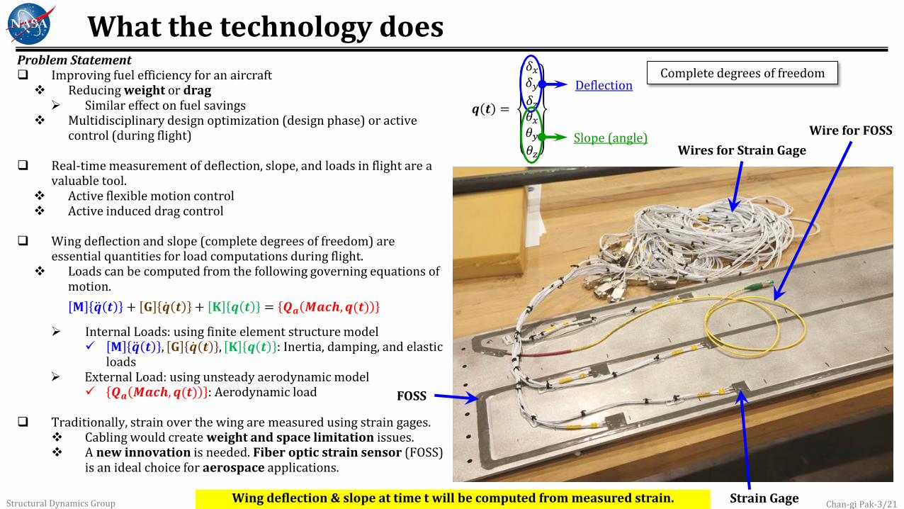
What the technology doesProblem Statement Improving fuel efficiency for an aircraft Reducing weight or drag Similar effect on fuel savings

Multidisciplinary design optimization (design phase) or active control (during flight)

Real-time measurement of deflection, slope, and loads in flight are a valuable tool.

Active flexible motion control Active induced drag control

Wing deflection and slope (complete degrees of freedom) are essential quantities for load computations during flight.

Loads can be computed from the following governing equations of motion.

Internal Loads: using finite element structure model 𝐌 𝒒 𝒕 , 𝐆 𝒒 𝒕 , 𝐊 𝒒 𝒕 : Inertia, damping, and elastic

loads External Load: using unsteady aerodynamic model

𝑸𝒂 𝑴𝒂𝒄𝒉, 𝒒(𝒕) : Aerodynamic load

Traditionally, strain over the wing are measured using strain gages. Cabling would create weight and space limitation issues. A new innovation is needed. Fiber optic strain sensor (FOSS)

is an ideal choice for aerospace applications.

𝐌 𝒒 𝒕 + 𝐆 𝒒 𝒕 + 𝐊 𝒒 𝒕 = 𝑸𝒂 𝑴𝒂𝒄𝒉, 𝒒(𝒕)

𝒒 𝒕 =

𝛿𝑥𝛿𝑦𝛿𝑧𝜃𝑥𝜃𝑦𝜃𝑧

Deflection

Slope (angle)

Complete degrees of freedom

Wing deflection & slope at time t will be computed from measured strain. Strain Gage

FOSS

Wires for Strain Gage

Wire for FOSS


Previous technologies Liu, T., Barrows, D. A., Burner, A. W., and Rhew, R. D., “Determining Aerodynamic Loads Based on Optical Deformation Measurements,” AIAA Journal,

Vol.40, No.6, June 2002, pp.1105-1112

NASA LRC; Application is limited for “beam”; static deflection & aerodynamic loads

Shkarayev, S., Krashantisa, R., and Tessler, A., “An Inverse Interpolation Method Utilizing In-Flight Strain Measurements for Determining Loads and

Structural Response of Aerospace Vehicles,” Proceedings of Third International Workshop on Structural Health Monitoring, 2001

University of Arizona and NASA LRC; “Full 3D” application; strain matching optimization; static deflection & loads

Kang, L.-H., Kim, D.-K., and Han, J.-H., “Estimation of Dynamic Structural Displacements using fiber Bragg grating strain sensors,” 2007

KAIST; displacement-strain-transformation (DST) matrix; Use strain mode shape; Application was based on beam structure; dynamic deflection

Igawa, H. et al., “Measurement of Distributed Strain and Load Identification Using 1500 mm Gauge Length FBG and Optical Frequency Domain

Reflectometry,” 20th International Conference on Optical Fibre Sensors, 2009

JAXA; using inverse analysis. “Beam” application only; static deflection & loads

Ko, W. and Richards, L., “Method for real-time structure shape-sensing,” US Patent #7520176B1, April 21, 2009

NASA AFRC; closed-form equations (based on beam theory); static deflection

Richards, L. and Ko, W. , “Process for using surface strain measurements to obtain operational loads for complex structures,” US Patent #7715994, May

11, 2010

NASA AFRC; “sectional” bending moment, torsional moment, and shear force along the “beam”.

Moore, J.P., “Method and Apparatus for Shape and End Position Determination using an Optical Fiber,” U.S. Patent No. 7813599, issued October 12, 2010

NASA LRC; curve-fitting; static deflection

Park, Y.-L. et al., “Real-Time Estimation of Three-Dimensional Needle Shape and Deflection for MRI-Guided Interventions,” IEEE/ASME Transactions on

Mechatronics, Vol. 15, No. 6, 2010, pp. 906-915

Harvard University, Stanford University, and Howard Hughes Medical Institute; Uses beam theory; static deflection & loads

Carpenter, T.J. and Albertani, R., “Aerodynamic Load Estimation from Virtual Strain Sensors for a Pliant Membrane Wing,” AIAA Journal, Vol.53, No.8,

August 2015, pp.2069-2079

Oregon State University; Aerodynamic loads are estimated from measured strain using virtual strain sensor technique.

Pak, C.-g., “Wing Shape Sensing from Measured Strain,” AIAA 2015-1427, AIAA Infotech @ Aerospace, Kissimmee, Florida, January 5-9, 2015; accepted

for publication on AIAA Journal (June 29, 2015); U.S. Patent Pending: Patent App No. 14/482784

NASA AFRC; “Full 3D” application; based on System Equivalent Reduction Expansion Process; static deflection


Measure Strain

Compute Wing

Deflection

Compute Wing

Deflection & Slope

Compute Loads

Technical features of two-step approach: Deflection ComputationProposed solutions: The method for obtaining the deflection over a flexible full 3D

aircraft structure was based on the following two steps. First Step: Compute wing deflection along fibers using measure

strain data Wing deflection will be computed along the fiber optic sensor line. Strains at selected locations will be “fitted”. These fitted strain will be integrated twice to have deflection

information. (Relative deflection w.r.t. the reference point) This is a finite element model independent method.

Second Step: Compute wing slope and deflection of entire structures Slope computation will be based on a finite element model

dependent technique. Wing deflection and slope will be computed at all the finite

element grid points.

First Step Second Step

𝒒 𝒕 =

𝛿𝑥(𝑡)𝛿𝑦(𝑡)

𝛿𝑧(𝑡)𝜃𝑥(𝑡)𝜃𝑦(𝑡)

𝜃𝑧(𝑡)휀𝑥(𝑡)

𝒒 𝒕

𝒒 𝒕 =

𝛿𝑥𝛿𝑦

𝛿𝑧(𝑡)𝜃𝑥𝜃𝑦𝜃𝑧

𝒒 𝒕

𝑸𝒂 𝑴𝒂𝒄𝒉, 𝒒(𝒕)

Loading analysis

Flight controller

Expansion module

Deflection analyzer

Assembler module

Fiber optic strain sensor

Strain

DeflectionDeflection and Slope

Drag and lift Acceleration

Velocity


Technical features of two-step approach : Deflection Computation (continued)

First Step Use piecewise least-squares method to minimize noise in the

measured strain data (strain/offset) Obtain cubic spline (Akima spline) function using re-generated

strain data points (assume small motion):

𝑑2𝛿𝑘𝑑𝑠2

= −𝜖𝑘(𝑠)/𝑐(𝑠)

Integrate fitted spline function to get slope data:

𝑑𝛿𝑘

𝑑𝑠= 𝜃𝑘 (𝑠)

Obtain cubic spline (Akima spline) function using computed slope data

Integrate fitted spline function to get deflection data: 𝛿𝑘(𝑠)

A measured strain is fitted using a piecewise least-squares curve fitting method together with the cubic spline technique.

DeflectionCurvature

-.007

-.006

-.005

-.004

-.003

-.002

-.001

.000

.001

0 10 20 30 40 50

Cu

rvatu

re, /i

n.

Along the fiber direction, in.

Piecewise least squares curve fit boundaries

: raw data

: direct curve fit

: curve fit after piecewise LS

Extrapolated data


𝒒𝑴𝒌

𝒒𝑺𝒌

𝒒𝑴𝒌

Technical features of two-step approach : Deflection Computation (continued)

Second Step: Based on General Transformation Definition of the generalized coordinates vector 𝒒 𝒌 and the othonormalized coordinates vector 𝜼 𝒌 at discrete time k

For all model reduction/expansion techniques, there is a relationship between the master (measured or tested) degrees of freedom and the slave (deleted or omitted) degrees of freedom which can be written in general terms as

Changing master DOF at discrete time k 𝒒𝑴 𝒌 to the corresponding measured values 𝒒𝑴 𝒌

Expansion of displacement using SEREP: kinds of least-squares surface fitting; most accurate reduction-expansion technique 𝒒𝑴𝒌 : master DOF at discrete time k; deflection along the fiber “computed from the first step”

𝒒𝑺𝒌 = 𝚽𝑺 𝚽𝑴𝑻 𝚽𝑴

−𝟏𝚽𝑴

𝑻 𝒒𝑴𝒌 : deflection and slope all over the structure

𝒒𝑴𝒌 = 𝚽𝑴 𝚽𝑴𝑻 𝚽𝑴

−𝟏𝚽𝑴

𝑻 𝒒𝑴𝒌 : smoothed master DOF

𝒒𝑴𝒌

𝒒𝑴𝒌

𝒒 𝒌 =𝒒𝑴𝒒𝑺 𝒌

= 𝚽 𝜼 𝒌 =𝚽𝑴

𝚽𝑺𝜼 𝒌

𝒒𝑴 𝒌 = 𝚽𝑴 𝜼 𝒌

𝒒𝑺 𝒌 = 𝚽𝑺 𝜼 𝒌

𝒒𝑴 𝒌 = 𝚽𝑴 𝜼 𝒌

𝜼 𝒌 = 𝚽𝑴𝑻 𝚽𝑴

−1𝚽𝑴

𝑻 𝒒𝑴 𝒌 𝒒 𝒌 =𝚽𝑴

𝚽𝑺𝚽𝑴

𝑻 𝚽𝑴−1

𝚽𝑴𝑻 𝒒𝑴 𝒌

𝚽𝑴𝑻 𝒒𝑴 𝒌 = 𝚽𝑴

𝑻 𝚽𝑴 𝜼 𝒌


Technical features of new technology: Acceleration Computation

From

Assume simple harmonic motion for normalized coordinates.

Acceleration at discrete time k can be expressed

Substituting Eq. (6) into (9) gives


=𝚽𝑴

𝚽𝑺𝜼 𝒌

Computed from unsteady strain distribution at a selected point using an on-line parameter estimation technique together with an AutoRegressive Moving Average (ARMA) model

Master DOF at discrete time k; deflection along the fiber “computed from the first step”

Basis function for least squares surface fitting: eigen function, comparison function, etc.

𝒒 𝒌 = 𝒒𝑴 𝒒𝑺 𝒌

=𝚽𝑴

𝚽𝑺 𝜼 𝒌

𝜂𝑖 𝑘 = −𝜔𝑖2𝜂𝑖 𝑘 𝑖 = 1,2,… , 𝑛

𝜼 𝒌 =

) 𝜂1(𝑘

) 𝜂2(𝑘⋮) 𝜂𝑛(𝑘

= −

𝜔12 0 … 0

0 𝜔22 … 0

00

00

⋱ ⋮… 𝜔𝑛

2

𝜂1 𝑘

𝜂2 𝑘⋮

𝜂𝑛 𝑘

= − 𝝎𝒊2 𝜼 𝒌 𝒒 𝒌 = −

𝚽𝑴 𝝎𝒊2

𝚽𝑺 𝝎𝒊2 𝜼 𝒌 𝐸𝑞. (9) 𝜼 𝒌 = 𝚽𝑴

𝑻 𝚽𝑴−1

𝚽𝑴𝑻 𝒒𝑴 𝒌 Eq. (6)

𝒒 𝒌 = −𝚽𝑴 𝝎𝒊

2

𝚽𝑺 𝝎𝒊2 𝚽𝑴

𝑻 𝚽𝑴−1


𝒒 𝒌 =𝚽𝑴

𝚽𝑺𝚽𝑴

𝑻 𝚽𝑴−1



Technical features of New Technology: Velocity Computation

From

Consider

Backward difference: has “phase shift” issue

Central difference: needs future response at time k

From linear AR model for the i-th orthonormalized coordinate

Future prediction 𝜂𝑖(𝑘 + 1) at time k

Central difference becomes

AR coefficients 𝑎1𝑖 & 𝑎2𝑖 for the i-th mode are computed from the i-th frequency 𝜔𝑖 which are estimated from the parameter estimation


=𝚽𝑴

𝚽𝑺𝜼 𝒌

𝜼 𝒌 =𝜼 𝒌+𝟏 − 𝜼 𝒌−𝟏

2Δ𝑡

𝜂𝑖(𝑘) = 𝑎1𝑖𝜂𝑖(𝑘 − 1) + 𝑎2𝑖𝜂𝑖(𝑘 − 2)

𝜂𝑖(𝑘) =𝑎1𝑖𝜂𝑖(𝑘) + 𝑎2𝑖 − 1 𝜂𝑖(𝑘 − 1)

2Δ𝑡


=𝚽𝑴

𝚽𝑺 𝜼 𝒌

𝜼 𝒌 =

𝜂1(𝑘) 𝜂2(𝑘)⋮ 𝜂𝑖(𝑘)


=𝚽𝑴

𝚽𝑺 𝜼 𝒌

𝜂𝑖(𝑘 + 1) = 𝑎1𝑖𝜂𝑖(𝑘) + 𝑎2𝑖𝜂𝑖(𝑘 − 1)

𝜂𝑖(𝑘) =𝑎1𝑖𝜂𝑖(𝑘) + 𝑎2𝑖 − 1 𝜂𝑖(𝑘 − 1)

2Δ𝑡 𝜼 𝒌 = 𝚽𝑴T 𝚽𝑴

−1𝚽𝑴

T 𝒒𝑴 𝒌

Computed from estimated frequenciesMaster DOF at discrete time k; deflection along

the fiber “computed from the first step”

Basis function for least squares surface fitting: eigen function, comparison function, etc.

𝒒 𝒌 =𝚽𝑴

𝚽𝑺𝚽𝑴

𝑻 𝚽𝑴−1


𝒒 𝒌 = −𝚽𝑴 𝝎𝒊

2


𝑻 𝚽𝑴−1


𝒒 𝒌 =𝚽𝑴 𝒋𝝎𝒊

𝚽𝑺 𝒋𝝎𝒊𝚽𝑴

𝑻 𝚽𝑴−1


???

𝜼 𝒌 =𝜼 𝒌 − 𝜼 𝒌−𝟏

Δ𝑡

Computational Validation

Cantilevered rectangular wing model


Grid 51

Grid 2601

Cantilevered Rectangular Wing Model Configuration of a wind tunnel test article

Has aluminum insert (thickness = 0.065 in ) covered with 6% circular arc cross-sectional shape (plastic foam)

Impulsive load is applied at the leading-edge of wing tip section MSC/NASTRAN sol 112: Modal transient response analysis

Compute strain Compute deflection & acceleration (target)

Two-step approach Compute deflection and acceleration from computed strain Compare computed deflection and acceleration with respect to

target values

21

1

3

5

7

9

11

13

15

17

19

Fiber

X11.5 in.

4.5

6 in

.

Fiber optic strain sensors: 11(upper) + 11(lower)

Y

22 Simulated FOSS locations

Applied load

Fibers Plate

elements

Strain plot elementRigid

element

Z

XA

A

0.065” aluminum insert

A-A

Flexible plastic foam

6% Circular arc


Model Tuning Idealization of the plastic foam weight

Case 1: equally smeared in aluminum plate.

Case 2: lumped mass weight are computed based on 6% circular-arc cross sectional shape.

Use structural dynamic model tuning technique

Chan-gi Pak and Samson Truong, “Creating a Test-Validated Finite-Element Model of the X-56A Aircraft Structure,” Journal of Aircraft, (2015), doi: http://arc.aiaa.org/doi/abs/10.2514/1.C033043

Mode Measured (Hz) Case 1 (Hz) % Error Case2 (Hz) % Error

1 14.29 15.09 5.6 14.29 0.0

2 80.41 77.40 -3.7 80.17 -0.3

3 89.80 93.57 4.2 89.04 -0.8

4 N/A 246.37 N/A 248.76 N/A

5 N/A 262.02 N/A 252.41 N/A

6 N/A 455.22 N/A 459.34 N/A

7 N/A 511.27 N/A 485.61 N/A

8 N/A 642.72 N/A 606.65 N/A

9 N/A 722.32 N/A 718.59 N/A

10 N/A 773.93 N/A 747.65 N/A

Properties Case 1 Model Case 2 Model

E 9847900 9207766

G 3639672 3836570

density 0.11166 0.1

Foam weight Smeared Lumped mass

Total weight 0.3806 lb 0.3806 lb

Xcg 2.28 inch 2.28 inch

Ycg 5.75 inch 5.75 inch

thickness 0.065 inch 0.065 inch

Measured vs. Computed FrequenciesDesign variables

Objective function: frequency error

0.065” aluminum insert Flexible plastic foam

6% Circular arc

http://arc.aiaa.org/doi/abs/10.2514/1.C033044


Mode Shapes

Mode 2: 80.17 HzMode 1: 14.29 Hz Mode 3: 89.04 Hz

Mode 5: 252.41 HzMode 4: 248.76 Hz


Two Sample Cases Case 1 computations

Case 1 properties are used to make the target responses. Use NASTRAN modal transient response analysis (sol112) 1200 time steps

Mode shapes from Case 1 are used to calculate transformation matrices. Mode shapes are eigen function.

Frequencies are estimated from strain data computed using Case 1 model.

Case 2 computations

Case 2 properties are used to make the target responses.

Use NASTRAN modal transient response analysis (sol112)

1200 time steps

Mode shapes from Case 1 are used to calculate transformation matrices.

Mode shapes are comparison function.

Case 1 model: Not validated model

Case 2 model: Validated model

Frequencies are estimated from strain data computed using Case 2 model.

Mode Measured (Hz) Case 1 (Hz) Case2 (Hz)

1 14.29 15.09 14.29

2 80.41 77.40 80.17

3 89.80 93.57 89.04

4 N/A 246.37 248.76

5 N/A 262.02 252.41

6 N/A 455.22 459.34

7 N/A 511.27 485.61

8 N/A 642.72 606.65

9 N/A 722.32 718.59

10 N/A 773.93 747.65From estimation

From Case 1 model (comparison function)

𝒒 𝒌 =𝚽𝑴

𝚽𝑺𝚽𝑴

𝑻 𝚽𝑴−1

𝚽𝑴𝑻 𝒒𝑴 𝒌 𝒒 𝒌 = −

𝚽𝑴 𝝎𝒊2


𝑻 𝚽𝑴−1


𝜼 𝒌 =

𝜂1(𝑘) 𝜂2(𝑘)⋮ 𝜂𝑖(𝑘)


=𝚽𝑴

𝚽𝑺 𝜼 𝒌

𝜂𝑖(𝑘) =𝑎1𝑖𝜂𝑖(𝑘) + 𝑎2𝑖 − 1 𝜂𝑖(𝑘 − 1)

2Δ𝑡

𝜼 𝒌 = 𝚽𝑴T 𝚽𝑴

−1𝚽𝑴

T 𝒒𝑴 𝒌

Comparison functions are used for Case 2


-1.5E-3

-1.0E-3

-5.0E-4

0.0E+0

5.0E-4

1.0E-3

1.5E-3

0.00 0.02 0.04 0.06 0.08 0.10

Str

ain

Time (sec)

Estimated System Frequencies: Case 1Mode Target (Hz) Estimated (Hz) % Error

1 15.09 15.09 0.00

2 77.40 77.40 0.00

3 93.57 93.57 0.00

4 246.37 246.37 0.00

5 262.02 262.02 0.00

6 455.22 455.22 0.00

7 511.27 511.27 0.00

8 642.72 642.72 0.00

9 722.32 722.32 0.00

10 773.93 773.93 0.00

Use Bierman’s U-D Factorization Algorithm Number of AR Coefficients = 20 Covariance matrix resetting interval = 80 time steps Forgetting factor = 0.98 Sampling time = 0.00062667 sec Nyquist frequency = 797.9 Hz Target frequencies & Time histories of strain: obtained from NASTRAN run

Strain values are obtained from the first element of the leading-edge fiber element located at the lower surface.

Strain value

Strain distribution @ T=0.188001 sec


Deflection Time Histories: Case 1

: Target: Current Method

Use eigen functions for the transformation matrices

22 fibers At grid 51

51

-0.05

-0.04

-0.03

-0.02

-0.01

0.00

0.01

0.02

0.03

0.04

0.05

0.00 0.01 0.02 0.03

Pit

ch

an

gle

(ra

dia

n)

Time (sec)

-0.3

-0.2

-0.1

0.0

0.1

0.2

0.3

0.00 0.02 0.04 0.06 0.08 0.10

Z d

efl

ecti

on

(in

ch

)

Time (sec)

-0.3

-0.2

-0.1

0.0

0.1

0.2

0.3

0.00 0.01 0.02 0.03

Z d

efl

ecti

on

(in

ch

)

Time (sec)

-0.05

-0.04

-0.03

-0.02

-0.01

0.00

0.01

0.02

0.03

0.04

0.05

0.00 0.02 0.04 0.06 0.08 0.10

Pit

ch

an

gle

(ra

dia

n)

Time (sec)


Acceleration Time Histories: Case 1

Use eigen functions for the transformation matrices

51



-6.E+5

-4.E+5

-2.E+5

0.E+0

2.E+5

4.E+5

6.E+5

0.00 0.01 0.02 0.03

Z a

ccele

rati

on

(in

ch

/sec^

2)

Time (sec)

-4.E+5

-3.E+5

-2.E+5

-1.E+5

0.E+0

1.E+5

2.E+5

3.E+5

4.E+5

0.00 0.01 0.02 0.03

Pit

ch

accele

rati

on

(ra

dia

n/s

ec^

2)

Time (sec)

-6.E+5

-4.E+5

-2.E+5

0.E+0

2.E+5

4.E+5

6.E+5

0.00 0.02 0.04 0.06 0.08 0.10

Z a

ccele

rati

on

(in

ch

/sec^

2)

Time (sec)

-4.E+5

-3.E+5

-2.E+5

-1.E+5

0.E+0

1.E+5

2.E+5

3.E+5

4.E+5

0.00 0.02 0.04 0.06 0.08 0.10

Pit

ch

accele

rati

on

(ra

dia

n/s

ec^

2)

Time (sec)


Velocity Time Histories: Case 1

51



-200

-150

-100

-50

0

50

100

150

200

0.00 0.01 0.02 0.03

Z v

elo

cit

y (

inch

/sec)

Time (sec)

-100

-80

-60

-40

-20

0

20

40

60

80

100

0.00 0.01 0.02 0.03

Pit

ch

rate

(in

ch

/sec)

Time (sec)

-200

-150

-100

-50

0

50

100

150

200

0.00 0.02 0.04 0.06 0.08 0.10

Z v

elo

cit

y (

inc

h/s

ec)

Time (sec)

-100

-80

-60

-40

-20

0

20

40

60

80

100

0.00 0.02 0.04 0.06 0.08 0.10

Pit

ch

rate

(in

ch

/sec)

Time (sec)


-1.5E-3

-1.0E-3

-5.0E-4

0.0E+0

5.0E-4

1.0E-3

1.5E-3

0.00 0.02 0.04 0.06 0.08 0.10

Str

ain

Time (sec)

Estimated System Frequencies: Case 2Mode Measured (Hz) Target (Hz) Estimated (Hz) % Error

1 14.29 14.29 14.28 -0.09

2 80.41 80.17 80.18 0.02

3 89.80 89.04 89.05 0.01

4 N/A 248.76 248.77 0.00

5 N/A 252.41 252.41 0.00

6 N/A 459.34 459.34 0.00

7 N/A 485.61 485.61 0.00

8 N/A 606.65 606.65 0.00

9 N/A 718.59 718.60 0.00

10 N/A 747.65 747.66 0.00

Use Bierman’s U-D Factorization Algorithm Number of AR Coefficients = 20 Covariance matrix resetting interval = 80 time steps Forgetting factor = 0.98 Sampling time = 0.0006487 sec Nyquist frequency = 770.8 Hz Target frequencies & Time histories of strain: obtained from NASTRAN run

Strain values are obtained from the first element of the leading-edge fiber element located at the lower surface.

Strain value

Strain distribution @ T=0.19461 sec

Chan-gi Pak-20/21Structural Dynamics Group Use comparison functions for the transformation matrices

Deflection Time Histories: Case 2: Target: Current Method

6, 10, & 22 fibers At grid 2601

2601

6 fibers

10 fibers

22 fibers

-0.05

-0.04

-0.03

-0.02

-0.01

0.00

0.01

0.02

0.03

0.04

0.05

0.00 0.01 0.02 0.03

Pit

ch

an

gle

(ra

dia

n)

Time (sec)

-0.25

-0.20

-0.15

-0.10

-0.05

0.00

0.05

0.10

0.15

0.20

0.25

0.00 0.01 0.02 0.03

Z d

efl

ecti

on

(in

ch

)

Time (sec)

-0.25

-0.20

-0.15

-0.10

-0.05

0.00

0.05

0.10

0.15

0.20

0.25

0.00 0.02 0.04 0.06 0.08 0.10

Z d

efl

ecti

on

(in

ch

)

Time (sec)

-0.05

-0.04

-0.03

-0.02

-0.01

0.00

0.01

0.02

0.03

0.04

0.05

0.00 0.02 0.04 0.06 0.08 0.10

Pit

ch

an

gle

(ra

dia

n)

Time (sec)

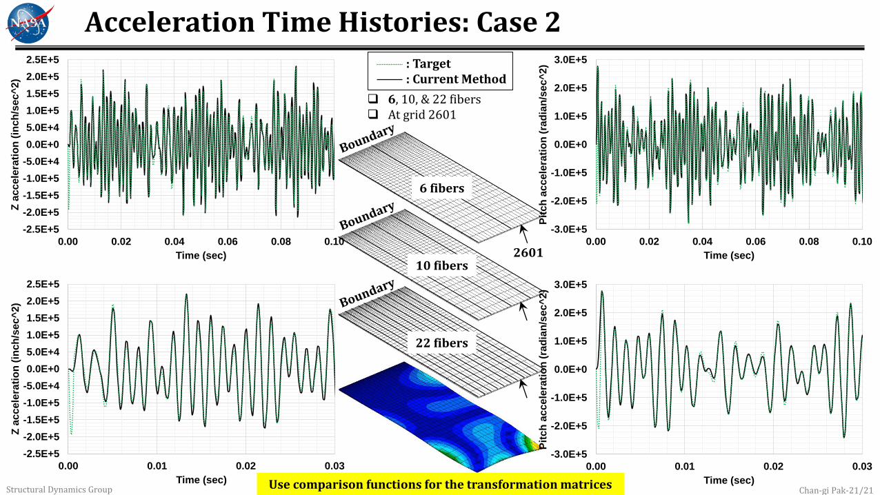
Chan-gi Pak-21/21Structural Dynamics Group Use comparison functions for the transformation matrices

Acceleration Time Histories: Case 2: Target: Current Method

6, 10, & 22 fibers At grid 2601

2601

6 fibers

10 fibers

22 fibers

-2.5E+5

-2.0E+5

-1.5E+5

-1.0E+5

-5.0E+4

0.0E+0

5.0E+4

1.0E+5

1.5E+5

2.0E+5

2.5E+5

0.00 0.01 0.02 0.03

Z a

cc

ele

rati

on

(in

ch

/sec

^2)

Time (sec)

-3.0E+5

-2.0E+5

-1.0E+5

0.0E+0

1.0E+5

2.0E+5

3.0E+5

0.00 0.01 0.02 0.03

Pit

ch

accele

rati

on

(ra

dia

n/s

ec^

2)

Time (sec)

-2.5E+5

-2.0E+5

-1.5E+5

-1.0E+5

-5.0E+4

0.0E+0

5.0E+4

1.0E+5

1.5E+5

2.0E+5

2.5E+5

0.00 0.02 0.04 0.06 0.08 0.10

Z a

cc

ele

rati

on

(in

ch

/se

c^

2)

Time (sec)

-3.0E+5

-2.0E+5

-1.0E+5

0.0E+0

1.0E+5

2.0E+5

3.0E+5

0.00 0.02 0.04 0.06 0.08 0.10

Pit

ch

accele

rati

on

(ra

dia

n/s

ec^

2)

Time (sec)


Velocity Time Histories: Case 2: Target: Current Method

6, 10, & 22 fibers At grid 2601

2601

6 fibers

10 fibers

22 fibers

-100

-80

-60

-40

-20

0

20

40

60

80

100

0.00 0.01 0.02 0.03

Z v

elo

cit

y (

inch

/sec)

Time (sec)

-80

-60

-40

-20

0

20

40

60

80

0.00 0.01 0.02 0.03

Pit

ch

ra

te (

rad

ian

/se

c)

Time (sec)

-100

-80

-60

-40

-20

0

20

40

60

80

100

0.00 0.02 0.04 0.06 0.08 0.10

Z v

elo

cit

y (

inc

h/s

ec)

Time (sec)

-80

-60

-40

-20

0

20

40

60

80

0.00 0.02 0.04 0.06 0.08 0.10

Pit

ch

ra

te (

rad

ian

/se

c)

Time (sec)


Summary of Computation Error

% Error ≡ 𝑘=0𝑛 Current approach 𝑘 −Target 𝑘

𝑘=0𝑛 Target 𝑘

Z deflection errors are the smallest

Z deflections are input for the second step.

Z deflections along the leading-edge fiber (grid 51) are input for the second step. (master DOF)

Pitch angle at grid 51 as well as Z deflection and pitch angle at grid 2601 are output from the second step. (slave DOF) Therefore, it’s less accurate than master DOFs.

Acceleration and velocity errors are bigger than the displacement errors.

Even six fibers also give good answer.

No big difference between 6, 10, & 22 fibers.

Model Grid (# of fiber)

% Error

Deflection Acceleration Velocity

Z Pitch Z Pitch Z Pitch

Case 1 51(22) 1.55 5.36 6.42 7.96 10.5 12.0

Case 2

2601(22) 1.38 5.76 16.9 9.84 15.0 11.4

2601(10) 1.67 5.99 17.0 10.2 15.9 11.7

2601(6) 1.79 6.35 17.6 10.2 19.0 11.8

6 fibers

2601

10 fibers

2601

22 fibers

2601


Conclusions

Acceleration and velocity of the cantilevered rectangular wing is successively obtained using the proposed approach.

Simple harmonic motion was assumed for the acceleration computations.

System frequencies are estimated from the time histories of strain measured at the leading-edge of the root section through the use of the parameter estimation technique together with the ARMA model.

The central difference equation with a linear AR model is used for the computations of velocity.

AR coefficients are computed using the estimated system frequencies.

Phase shift issue associated with the backward difference equation are overcome with the proposed approach.

The total of six fibers provides the good results.

Quality of results based on 6, 10, and 22 fibers are similar.

Questions ?

Acceleration and Velocity Sensing from Measured Strain · Acceleration and Velocity Sensing from...

Documents

Transcript of Acceleration and Velocity Sensing from Measured Strain · Acceleration and Velocity Sensing from...