Abundance Estimates for Game Ducks in Victoria
41
OFFICIAL Arthur Rylah Institute for Environmental Research Technical Report Series No. 325 Abundance Estimates for Game Ducks in Victoria Results from the 2020 Aerial Survey D.S.L. Ramsey and B. Fanson April 2021
Transcript of Abundance Estimates for Game Ducks in Victoria

OFFICIAL
Arthur Rylah Institute for Environmental Research
Technical Report Series No. 325
Abundance Estimates for
Game Ducks in Victoria
Results from the 2020 Aerial Survey
D.S.L. Ramsey and B. Fanson
April 2021

Arthur Rylah Institute for Environmental Research
Department of Environment, Land, Water and Planning
PO Box 137
Heidelberg, Victoria 3084
Phone (03) 9450 8600
Website: www.ari.vic.gov.au
Citation: Ramsey, D.S.L. and Fanson, B. (2021). Abundance estimates of game ducks in Victoria: Results from the 2020 aerial
survey. Arthur Rylah Institute for Environmental Research Technical Report Series No. 325. Department of Environment, Land,
Water and Planning, Heidelberg, Victoria.
Front cover photo: Male Hardhead (Aythya australis) (Source: Wikimedia).
© The State of Victoria Department of Environment, Land, Water and Planning 2021
This work is licensed under a Creative Commons Attribution 3.0 Australia licence. You are free to re-use the work under that licence,
on the condition that you credit the State of Victoria as author. The licence does not apply to any images, photographs or branding,
including the Victorian Coat of Arms, the Victorian Government logo, the Department of Environment, Land, Water and Planning logo
and the Arthur Rylah Institute logo. To view a copy of this licence, visit http://creativecommons.org/licenses/by/3.0/au/deed.en
ISSN 1835-3827 (print)
ISSN 1835-3835 (pdf))
ISBN 978-1-76105-488-4 (Print)
ISBN 978-1-76105-489-1 (pdf/online/MS word)
Disclaimer
This publication may be of assistance to you but the State of Victoria and its employees do not guarantee that the publication is
without flaw of any kind or is wholly appropriate for your particular purposes and therefore disclaims all liability for any error, loss or
other consequence which may arise from you relying on any information in this publication.
Accessibility
If you would like to receive this publication in an alternative format, please
telephone the DELWP Customer Service Centre on 136 186, email
[email protected] or contact us via the National Relay
Service on 133 677 or www.relayservice.com.au. This document is also
available on the internet at www.delwp.vic.gov.au
Acknowledgment
We acknowledge and respect Victorian Traditional Owners as the original custodians of Victoria's land and waters, their unique ability to care for Country and deep spiritual connection to it. We honour Elders past and present whose knowledge and wisdom has ensured the continuation of culture and traditional practices.
We are committed to genuinely partner, and meaningfully engage, with Victoria's Traditional Owners and Aboriginal communities to support the protection of Country, the maintenance of spiritual and cultural practices and their broader aspirations in the 21st century and beyond.

Arthur Rylah Institute for Environmental Research
Department of Environment, Land, Water and Planning
Heidelberg, Victoria
Abundance Estimates of Game Ducks in
Victoria: Results from the 2020 Aerial
Survey
David S.L. Ramsey and Ben Fanson
Arthur Rylah Institute for Environmental Research
123 Brown Street, Heidelberg, Victoria 3084
Date
Arthur Rylah Institute for Environmental Research Technical Report Series No. 325

Game duck abundance in Victoria 2020 ii
Acknowledgements
Aerial surveys were conducted by Terrestrial Ecosystem Services Pty Ltd (www.ecoknowledge.com.au). We
would like to thank Mark Lethbridge of Terrestrial Ecosystem Services for providing additional support and
valuable feedback on the aerial survey data. The authors thank Simon Toop, Michael Scroggie and Peter
Menkhorst for providing valuable comments on a draft of this report.

Game duck abundance in Victoria 2020 1
Contents
Acknowledgements ii
Summary 2
1 Introduction 4
1.1 Objectives 4
2 Methods 5
2.1 Estimates of surface water availability 5
2.1.1 Creating the farm dam layer 6
2.1.2 Creating the waterbody surface water layer 7
2.2 Selecting the sample of waterbodies 8
2.2.1 Assigning waterbody objects to primary sampling units 8
2.2.2 Selecting the sampling frame 8
2.2.3 Selecting the sample 8
2.3 Aerial sampling of game ducks 9
2.4 Abundance estimation 10
2.4.1 Statewide abundance estimates 11
2.4.2 Utility of the model-based approach 11
2.4.3 Adjustments to the sampling design 12
2.5 Estimates of seasonal harvest arrangements 12
3 Results 13
3.1 Aerial survey summary 13
3.2 Surface water availability 13
3.3 Game duck abundance estimates 15
3.4 Statewide abundance estimates 17
3.4.1 Design-based estimates 17
3.4.2 Model-based estimates 18
3.4.3 Utility of the model-based approach 20
3.4.4 Adjustments to the sampling design 21
3.5 Seasonal harvest regulations 22
4 Discussion 24
4.1 Recommendations 25
References 27
Appendix A 29
Appendix B 31
Appendix C 36

2 Game duck abundance in Victoria 2020
Summary
Context:
In Victoria, eight species of native duck are subject to legal recreational harvest: Grey Teal (Anas gracilis),
Pacific Black Duck (Anas superciliosa), Australian Wood Duck (Chenonetta jubata), Australian Shelduck
(Tadorna tadornoides), Pink-eared Duck (Malacorhynchus membranaceus), Chestnut Teal (Anas castanea),
Hardhead (Aythya australis) and Australasian Shoveler (Spatula rhynchotis) (hereafter called game ducks).
Comprehensive surveys in Victoria suitable for estimating the statewide abundance of game duck species
are lacking, but are vital if an adaptive harvest management framework is to be adopted for managing
recreational harvest. A recent study identified survey methods and a sampling design that would be suitable
for estimating the abundance of game ducks on waterbodies in Victoria (Ramsey 2020). The survey design
involved independent counts by two observers in a helicopter from at least 600 randomly selected
waterbodies, including small farm dams, using a two-stage sampling design with the first stage consisting of
hexagonal primary units with a 10 km minimal diameter (87 km2). A pilot study was subsequently
undertaken in November 2020 to assess the suitability of the survey design under actual conditions.
Aims:
The aim of this study was to conduct an analysis of the pilot aerial survey to determine whether the data
were suitable for providing robust estimates of the abundance of game ducks. This included a detailed
evaluation of the survey results to identify possible improvements to the sampling design to increase the
confidence in the survey results. Investigation was also undertaken on the use of the abundance estimates
for the setting of the annual seasonal duck hunting arrangements.
Methods:
Estimates of surface water on waterbodies in Victoria (wetlands, dams and sewage treatment ponds, but not
watercourses) were derived from Landsat and Sentinel-2 raster imagery for the extended spring period to
derive a sampling frame, which was then used to select a random sample of waterbodies for aerial survey.
Aerial sampling of each waterbody was undertaken from a helicopter, with two observers on the left side of
the aircraft (one forward and one rear) conducting counts of game ducks at each waterbody independently.
The abundance of game duck species at each sampled waterbody was estimated using a zero-inflated N-
mixture model with Bayesian inference. Design-based and model-based procedures were then used to
estimate total abundance for the entire sampling frame to derive statewide estimates of abundance for each
game duck species. Simulations were also undertaken to determine the improvement on the precision of
abundance estimates when more waterbodies were added to the sample. The utility of the model-based
approach was also tested by using it to predict the abundance of game ducks in the Riverina district of New
South Wales, and then comparing these predictions to recent independent estimates from that region.
Data on the size of the total game duck harvest, estimated from telephone surveys of hunters from 2009 to
2019, was used to estimate the relationship between total duck harvest, seasonal arrangements (season
length and daily bag limit) and number of licensed hunters. This relationship was then used to find
combinations of season length and daily bag limit that would be consistent with a conservative recreational
harvest rate of 10% of the estimated total game duck population.
Results:
A total of 653 waterbodies were subject to aerial survey including 540 dams, 2 sewage treatment ponds and
111 wetlands. Many of the waterbodies initially selected, but especially sewage ponds, could not be
sampled due to the risks associated with the proximity of high-tension power lines, windfarms or built-up
areas. Design-based estimates of total abundance indicated that the population of game ducks on dams
and wetlands in Victoria was 2 452 100 (95% confidence interval: 1 840 400 – 3,267,000). Teal (Grey and
Chestnut Teal combined) were the most numerous game species (c. 981,000), followed by Wood Duck (c.
690,000), Australian Shelduck (c. 407,000), Pacific Black Duck (c. 328,000) and Hardhead (c. 55,000). The
relative precision of estimates for individual species varied, being most precise for Pacific Black Duck (0.2),
and least precise for Hardhead (0.51). Model-based estimates were similar to the design-based ones, with a
total estimate of 2,348,100 game ducks. However, model-based estimates tended to be more precise than

Game duck abundance in Victoria 2020 3
the corresponding design-based estimates. The majority of game ducks occurred on small farm dams (up to
6 ha), especially Wood Duck and teal. Teal and Australian Shelduck were also found in substantial numbers
in larger wetlands.
Using the model-based approach to predict game duck abundances to the Riverina produced mixed results.
Estimates for teal and Wood Duck were comparable to independently derived estimates having a relative
bias of < 20%. However, results for Pacific Black Duck, Australian Shelduck and Hardhead were highly
biased, indicating that the model was inadequate for predicting the abundance of these species outside
Victoria.
For the desired harvest quota of 10% of the estimated total game duck abundance (i.e., 245,200), the
corresponding estimates of bag limit and season length suggests that a season length of 75 days and a bag
limit of 5 would be consistent with this harvest quota. However, other combinations of season length and
bag limit were also compatible with this level of offtake.
Conclusions and implications:
The pilot aerial survey has provided the first robust estimates of the abundance of game ducks across
Victoria. Although the estimates presented here account for the major sources of variation in duck
abundances, such as habitat availability (surface water estimates) and observer error (detection probability),
some adjustment to the sample sizes of each type of waterbody is warranted to increase the precision of the
abundance estimates for individual species. These are detailed in the recommendations.
Estimates of statewide abundance of game ducks, such as those detailed here, would be suitable as a basis
for setting more rigorous and transparent recreational harvest arrangements. Moreover, regular estimates of
statewide abundance will be essential if Victoria is to adopt adaptive harvest management as the basis for
maintaining the sustainability of recreational duck hunting.
Recommendations
To improve the Victorian game duck survey to provide more robust estimates of abundance that will be
suitable for setting the annual seasonal arrangements for recreational duck hunting, the following changes
are recommended:
• Increase the number of sampled waterbodies in the two-stage sampling design to 1300 by sampling 90
primary units and 15 waterbodies per primary unit.
• Alternatively, sample 800 waterbodies using single-stage stratified random sampling, as this should lead
to more precise abundance estimates than two-stage sampling. However, only adopt this option if
logistically and financially feasible.
• Following sample selection, implement alternative sampling methods for waterbodies where it is not
feasible to conduct aerial surveys from a helicopter. Smaller waterbodies (up to 6 ha) should be
sampled simultaneously by two ground observers recording independently with the aid of a spotting
scope, while larger waterbodies (more than 6 ha) should be sampled by an unmanned aerial vehicle
(UAV) recording high resolution video (i.e., 4K at 60 fps).
• Modify the survey design to include waterways (i.e. rivers, large streams and irrigation channels). This
can be achieved by including waterways in either the two-stage or single-stage sampling design.
• To provide separate estimates for Grey and Chestnut Teal from aerial surveys, conduct ground surveys
targeting teal at sites around the coast as well as north of the Princess Highway/Freeway to obtain an
estimate of the sex ratio for both teal species.
• To improve model-based estimates of duck abundance, investigate additional variables, such as
landuse, waterbody proximity or climate variables, that may better describe variation in duck abundance
to provide more confidence in model-based predictions.
• To improve the model of the relationship between total duck harvest and annual seasonal arrangements,
investigate additional variables that more accurately reflect hunting effort, which should lead to improved
estimates of daily bag limits and season length to achieve the desired harvest quota.

4 Game duck abundance in Victoria 2020
1 Introduction
In Victoria, eight species of native duck are subject to legal harvest: Grey Teal (Anas gracilis), Pacific Black
Duck (Anas superciliosa), Australian Wood Duck (Chenonetta jubata), Australian Shelduck (Tadorna
tadornoides), Pink-eared Duck (Malacorhynchus membranaceus), Chestnut Teal (Anas castanea), Hardhead
(Aythya australis) and Australasian Shoveler (Spatula rhynchotis). The Victorian government manages
recreational duck hunting sustainably by setting seasonal daily bag limits for each species, as well as the
timing of the start and end of the hunting season (i.e. season length). These arrangements can change each
year, depending on the information available about the status of populations and the prevailing
environmental conditions. The main source of information used to inform the population status of game
ducks is the Eastern Australian Waterbird Survey (EAWS) (Kingsford and Porter 2009). There is also some
reliance on regional game duck surveys conducted in parts of South Australia (DEWNR 2016) and the
Riverina district of New South Wales (Dundas et al. 2019). The Victorian Priority Waterbird Count
(Menkhorst and Purdey 2016) includes annual surveys of up to 200 wetlands across Victoria. However,
these surveys are conducted just before the start of the hunting season and are used primarily for identifying
locations of threatened species or breeding colonies that may warrant more careful management, including
closure to hunting.
Comprehensive surveys for estimating the statewide abundance of game duck species are vital if an
adaptive harvest management framework (e.g. Nichols et al. 2007) is to be adopted for managing the
recreational harvest of game ducks (Ramsey et al. 2017). However, the Victorian Priority Waterbird Count
and EAWS surveys have inadequate coverage and/or sampling designs for Victorian waterbodies to enable
a robust estimation of duck abundances. In addition, these surveys also have other drawbacks including
being unable to account for birds missed by observers (imperfect detection) and being unsuitable for the
detection of species inhabiting smaller waterbodies such as farm dams. In addition to undertaking surveys at
a sample of waterbodies, estimation of the abundance of game ducks across the state would also require an
estimate of the availability of surface water for each of the waterbody types around the period when the
surveys were undertaken. Surface water can now be routinely detected using appropriate algorithms applied
to satellite imagery (e.g. Pekel et al. 2016; Mueller et al. 2016).
A recent study identified survey methods and a sampling design that would be suitable for estimating the
abundances of games ducks on waterbodies in Victoria (Ramsey 2020). The survey design involves double
observer counts from a helicopter from at least 600 randomly selected waterbodies, including small farm
dams. Waterbodies were stratified into type (wetlands, dams, sewage treatment ponds) and size classes
(< 6 ha, 6–50 ha, > 50 ha). A two-stage sampling design was recommended, with waterbodies partitioned
into primary units on a hexagonal grid with a cell size of 10 km minimal diameter (area 87 km2), with both
primary units and waterbodies within selected primary units subject to random sampling (see Ramsey 2020
for more details on the sampling design). That study further recommended that a pilot study be undertaken
to assess the performance of the survey design and observation methods in order to refine the
recommended survey design. The Victorian Game Management Authority carried out a pilot study of this
methodology, covering 650 waterbodies, in November 2020.
1.1 Objectives
The aim of this study was to conduct an analysis of the pilot study data to determine whether the data could
provide robust estimates of the abundance for each species of game duck. This was to be achieved through
the following objectives:
• Estimate the current amount of surface water available for use by game ducks within Victoria using the
most recent satellite imagery (LandSat and Sentinel2) combined with vector layers of waterbodies
(including farm dams).
• Conduct an analysis of the aerial survey data from the pilot study in conjunction with the estimates of
surface water availability to estimate the abundance and distribution of each game duck species in
Victoria.
Game duck abundance in Victoria 2020 5
• Identify modifications to the aerial survey design that would lead to improvements in the statewide
estimates, if required.
• Evaluate the predictive ability of model-based estimates of game duck abundances using additional
monitoring data on game ducks collected in the Riverina district of New South Wales.
2 Methods
2.1 Estimates of surface water availability
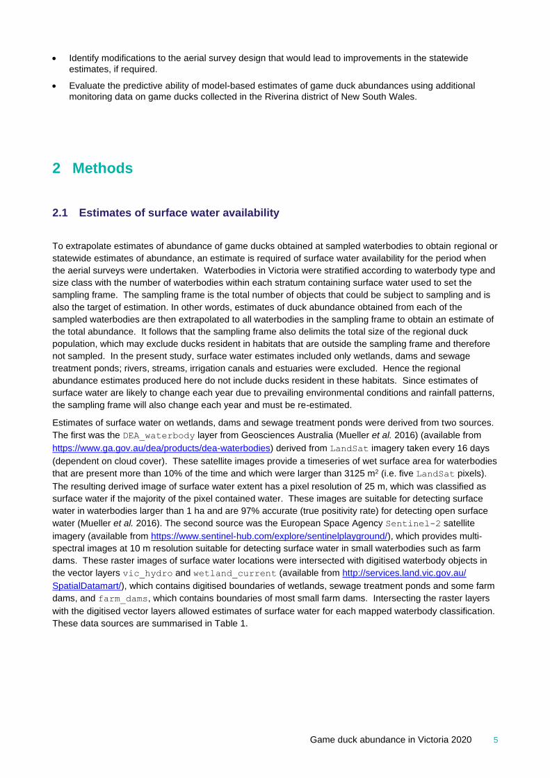
To extrapolate estimates of abundance of game ducks obtained at sampled waterbodies to obtain regional or
statewide estimates of abundance, an estimate is required of surface water availability for the period when
the aerial surveys were undertaken. Waterbodies in Victoria were stratified according to waterbody type and
size class with the number of waterbodies within each stratum containing surface water used to set the
sampling frame. The sampling frame is the total number of objects that could be subject to sampling and is
also the target of estimation. In other words, estimates of duck abundance obtained from each of the
sampled waterbodies are then extrapolated to all waterbodies in the sampling frame to obtain an estimate of
the total abundance. It follows that the sampling frame also delimits the total size of the regional duck
population, which may exclude ducks resident in habitats that are outside the sampling frame and therefore
not sampled. In the present study, surface water estimates included only wetlands, dams and sewage
treatment ponds; rivers, streams, irrigation canals and estuaries were excluded. Hence the regional
abundance estimates produced here do not include ducks resident in these habitats. Since estimates of
surface water are likely to change each year due to prevailing environmental conditions and rainfall patterns,
the sampling frame will also change each year and must be re-estimated.
Estimates of surface water on wetlands, dams and sewage treatment ponds were derived from two sources.
The first was the DEA_waterbody layer from Geosciences Australia (Mueller et al. 2016) (available from
https://www.ga.gov.au/dea/products/dea-waterbodies) derived from LandSat imagery taken every 16 days
(dependent on cloud cover). These satellite images provide a timeseries of wet surface area for waterbodies
that are present more than 10% of the time and which were larger than 3125 m2 (i.e. five LandSat pixels).
The resulting derived image of surface water extent has a pixel resolution of 25 m, which was classified as
surface water if the majority of the pixel contained water. These images are suitable for detecting surface
water in waterbodies larger than 1 ha and are 97% accurate (true positivity rate) for detecting open surface
water (Mueller et al. 2016). The second source was the European Space Agency Sentinel-2 satellite
imagery (available from https://www.sentinel-hub.com/explore/sentinelplayground/), which provides multi-
spectral images at 10 m resolution suitable for detecting surface water in small waterbodies such as farm
dams. These raster images of surface water locations were intersected with digitised waterbody objects in
the vector layers vic_hydro and wetland_current (available from http://services.land.vic.gov.au/
SpatialDatamart/), which contains digitised boundaries of wetlands, sewage treatment ponds and some farm
dams, and farm_dams, which contains boundaries of most small farm dams. Intersecting the raster layers
with the digitised vector layers allowed estimates of surface water for each mapped waterbody classification.
These data sources are summarised in Table 1.

6 Game duck abundance in Victoria 2020
Table 1. Summary of datasets used to create surface water estimates for Victoria.
Layer name Type Source Method Notes
vic_hydro Vector DEWLP satellite and
aerial
Digitised boundaries of all artificial
waterbodies (including farm dams) in
southern Victoria and all larger artificial
waterbodies in northern Victoria using
a combination of satellite and aerial
imagery. Last updated in January
2019.
wetland_current Vector DELWP Aerial Polygons showing the extent and types
of wetlands in Victoria. Wetland
Current was created in 2013 and
updated in 2014. Wetlands were
classified (according to the new
classification framework) into primary
categories based on wetland system
type, salinity regime, water regime,
water source, dominant vegetation and
wetland origin.
farm_dams Vector DELWP Satellite and
aerial
Digitised boundaries of all man-made
farm dams (< 6 ha) in Victoria
DEA waterbody Raster Geosciences
Australia
Landsat imagery
every 16 days,
depending on
cloud cover; if
>10% cloud, then
missing
Wet surface area for waterbodies that
are present more than 10% of the time
and are larger than 3125 m2 (5
Landsat pixels). Water classification is
based on the Tasseled Cap Wetness
metric (Jin and Sader 2005).
Sentinel-2 Raster ESA Satellite imagery
every 5 days
(depending on
cloud cover)
Green and near-infrared bands used to
construct Normalised Difference Water
Index (NDWI) (Mueller et al. 2016)
indicating surface water at 10 m
resolution. Used to indicate the
presence of surface water in small
farm dams (less than 1 ha).
2.1.1 Creating the farm dam layer
Farm dams were abundant and their mapped locations were contained in the farm_dam and
vicmap_hydro vector layers. We estimated the concordance between these layers by calculating the
overlap of dams between the two layers (Figure 1). Overall, concordance was moderate (~65%). It should
also be noted that the documentation for vicmap_hydro states that 70% of the farm dams in Victoria are
included (Vicmap Hydro product data description, 2018). Assuming this 70% estimate is correct, the
estimated number of farm dams in Victoria is 555 764, or 166 729 extra dams not mapped. The farm_dam
layer had an extra 127 299, which could account for 76% of those extra farm dams. The final combined layer
contained 509 737 farm dams, which together accounted for 93% of farm dams. (Table 2).

Game duck abundance in Victoria 2020 7
Figure 1. Example of farm_dam layer (blue polygons) and vicmap_hydro_point layer (yellow dots) showing
partial overlap.
2.1.2 Creating the waterbody surface water layer
The DEA_waterbody raster layer of surface water presence was first clipped, keeping only spatial objects in
Victoria. This resulted in 19,740 objects. As the DEA_waterbody layer did not have waterbody
classifications, we intersected the other vector layers wetland_current, vicmap_hydro and farm_dam
and used the appropriate attributes to classify each waterbody based on the type (wetland, dam or sewage
treatment pond) as well as a size class (< 6 ha, 6–50 ha, > 50 ha) (Figure 2). Objects classified as
watercourses (i.e. rivers, streams, estuaries, irrigation channels) were not included. Sewage treatment plants
containing multiple polygons (representing separate ponds) were combined into a single object. This final
layer contained 9 715 waterbody objects (Table 2).
Using this layer, we obtained the most recent wet proportion for each object as well as the average of the
three most recent observations. Additionally, for every object we calculated the proportion of times in the
‘extended spring’ period (October to January) that the object had water in the past 30 years.
Figure 2: Example of DEA layer (blue polygons) compared to vicmap_hydro_point (yellow polygons in the left
figure) and current_wetland layer (green polygons in the right figure).

8 Game duck abundance in Victoria 2020
Table 2: Number of waterbodies within each waterbody type and size class from the
combined vector layers listed in Table 1.
Waterbody type Size class (max) n
Dam < 6 ha 509 737
6–50 ha 52
Sewage ponds < 6 ha 31
6–50 ha 31
> 50 ha 7
Wetlands < 6 ha 7 098
6–50 ha 1 978
> 50 ha 518
Total 519 452
2.2 Selecting the sample of waterbodies
2.2.1 Assigning waterbody objects to primary sampling units
Primary sampling units were created across Victoria using a hexagonal grid (hexagon minimal diameter = 10
km, area = 87 km2) across the state. Each waterbody object was then assigned to a primary unit. If an object
overlapped multiple hexagons, the object was assigned to the hexagon that encompassed the highest
percentage of the objects area (if tied, then the first hexagon was picked for the assignment). It should be
noted that this method used the maximum water extent of the object (the DEA polygon) to calculate polygon
area and it was also possible that during drier periods no surface water was in the chosen hexagon.
2.2.2 Selecting the sampling frame
To help determine whether objects in the waterbody layer contained surface water during spring, just prior to
the aerial surveys, we selected the DEA waterbodies that historically held water more than 40% of the time in
the extended spring period or had more than 10% water based on the last Landsat image. All farm dams
were initially included in the initial sampling frame. Following the aerial survey we observed the presence or
absence of surface water in each of the sampled waterbodies. We used this information to refine the
sampling frame by calibrating the Normalised Difference Water Index (NDWI) calculated from the imagery for
both the DEA waterbody layer (larger waterbodies) and Sentinel-2 layer (small farm dams) by using the
observed presence or absence of water as a training set. The NDWI threshold was then set for both the
DEA and Sentinel-2 derived NDWI that maximised the training accuracy (proportion of both observed wet
and dry waterbodies that were correctly predicted).
2.2.3 Selecting the sample
Sample selection was as described in Ramsey (2020), using the estimate of the sampling frame described
above. An initial sample of 110 primary units were selected from the sampling frame with inclusion
probabilities proportional to the number of waterbodies larger than 50 ha within the unit. Within each
selected primary unit, up to 10 secondary units were selected using proportional representation based on
waterbody type and size class. A total of 1259 waterbodies were initially selected for sampling (Table 3,
Figure 3), which was more than the nominal amount required (about 600) due to the fact that some
waterbodies would not be available for aerial sampling due to airspace restrictions (e.g. proximity to built-up
areas) or the need to avoid areas with high-tension power lines.

Game duck abundance in Victoria 2020 9
Table 3: Summary of initial random sample of waterbodies within each selected primary unit
by waterbody type and size class.
Waterbody type Size class Number
Dams < 6 ha 972
6–50 ha 1
Sewage ponds < 6 ha 1
6–50 ha 8
Wetlands < 6 ha 203
6–50 ha 40
> 50 ha 34
Total 1259
Figure 3. Locations of the initial sample of waterbodies selected for aerial surveys. Waterbodies were selected
from 110 primary units with an unequal probability selection design. Bioregion boundaries are (clockwise from
top left), West, North, East and South.
2.3 Aerial sampling of game ducks
Aerial sampling of each waterbody was undertaken from a Squirrel AS-350 helicopter. Two observers on the
left side of the aircraft (one forward and one rear) conducted counts of game ducks at each waterbody
independently. For smaller waterbodies and farm dams, each waterbody was approached, and counts
conducted while the aircraft completed a low circuit around the waterbody circumference at a height of
around 30–50 m. For eight of the larger waterbodies (> 50 ha), only a portion of the waterbody (selected at
random) was surveyed, and the proportion of the surface area searched was recorded using GPS. The
counts for each observer for the entire surface area were then imputed using the proportion of the waterbody
surveyed.

10 Game duck abundance in Victoria 2020
2.4 Abundance estimation
2.4.1 Waterbody level estimates
The two independent replicate counts of game ducks at each sampled waterbody can be used to estimate
the abundance of ducks at each waterbody, corrected for imperfect detection (birds missed by the observers)
using an N-mixture model (Royle 2004). The N-mixture model has two components: an abundance
component, representing the true (but unknown) number of ducks present on each waterbody at the time of
the survey, and a detection component, representing the measurement (detection) error consisting of an
estimate of the fraction of birds that were present but missed by the observers. The abundance component
can also be a function of covariates likely to explain variation in abundance between waterbodies, such as
waterbody type, size class and geographic region. Likewise, the detection component can also depend on
covariates that affect the detection process, such as the presence of vegetation or glare from the water
surface. The standard N-mixture model can also be extended to account for extra spatial heterogeneity such
as the presence of excess zeros in the count data, caused by some waterbodies being unsuitable for ducks
at the time of the survey. Here, adopting a zero-inflated distribution such as a zero-inflated Poisson (ZIP)
enables the N-mixture model to account for excess zeros by modelling the probability of duck presence on
each waterbody. Hence, the count data (containing excess zeros) are now modelled as being subject to
three random processes, the probability that ducks were present on the waterbody, the abundance of ducks,
given that ducks were present and the probability of being observed, given ducks were present. Like the
abundance and detection probability parameters, the probability of presence can also be modelled with
covariate values.
To account for all these potential sources of variation in the aerial counts of game ducks, we fitted an N-
mixture ZIP model to the data on each sampled waterbody using the following model definition:
𝑦𝑠𝑖𝑡 ~ Binomial(𝑛𝑠𝑖 , 𝑝𝑖𝑡) (𝐸𝑞𝑢𝑎𝑡𝑖𝑜𝑛 1)
𝑛𝑠𝑖 ~ Poisson(𝜆𝑠𝑖 𝑃𝑠𝑖)
𝑃𝑠𝑖~ Bernoulli(𝜓𝑠𝑖)
log(𝜆𝑠𝑖) = 𝛽0,s + 𝜁𝑘,𝑠𝑇𝑖 + 𝜃𝑙,𝑠𝑆𝑖 + 𝛿𝑟,𝑠𝑅𝑖
logit(𝜓𝑠𝑖) = 𝛾0,s + 𝜂𝑘,𝑠𝑇𝑖 + 𝜍𝑙,𝑠𝑆𝑖 + 𝜏𝑟,𝑠𝑅𝑖
logit(𝑝𝑖𝑡) = 𝛼0 + 𝜐𝑔𝐺𝑖 + 𝜌ℎ𝐻𝑖
Where 𝑦𝑠𝑖𝑡 is the aerial count for duck species 𝑠 at waterbody 𝑖 for observer 𝑡, which was a binomial random
variable given the true abundance 𝑛𝑠𝑖 for species 𝑠 on waterbody 𝑖 and detection probability 𝑝𝑖𝑡. The latent
abundance (𝑛𝑠𝑖) was assumed to be Poisson distributed with rate 𝜆𝑠𝑖 if 𝑃𝑠𝑖 was equal to 1 with probability 𝜓𝑠𝑖
and zero otherwise with probability (1 − 𝜓𝑠𝑖). Covariates affecting abundance were waterbody type 𝑇, size
class 𝑆 and bioregion 𝑅.
The probability of presence was considered to depend on the same set of attributes, while the detection
probability was modelled as a function of the presence of glare from the water surface 𝐺 and habitat type 𝐻
(open, reeds or woodland). The parameters 𝛽0, 𝛼0, 𝛾0 were the intercepts while 𝜁, 𝜃, 𝛿, 𝜂, 𝜍, 𝜏, 𝜐 and 𝜌 were
the parameters for the respective covariates in the linear models. The parameters for the covariates on
abundance and presence probability were estimated separately for each duck species, indicated by the
subscript 𝑠 and had levels subscripted by 𝑘, 𝑙, or 𝑟 as indicated in Equation 1. The model in Equation 1 was
estimated in a Bayesian framework using Hamiltonian Markov Chain Monte Carlo methods in Stan (version
2.21.2) from within R using RStan (Carpenter et al. 2017). Weakly informative prior distributions were used
for all parameters in the model specified as 𝑁(0, 5). A total of 3000 MCMC iterations were run for the model
using 5 chains with the first 1000 iterations considered to be ‘warmup’ (tuning) iterations and discarded. This
left a total of 10,000 samples remaining for each parameter to form inference.

Game duck abundance in Victoria 2020 11
2.4.2 Statewide abundance estimates
Predictions of game duck abundance for the entire sampling frame (i.e. waterbodies containing water within
Victoria) were made using a design-based approach (Thompson 1992). Design-based estimates of total
abundance proceeded by using predicted abundance �̂�𝑖 for each sampled waterbody (𝑖 = 1, … , 𝑤𝑠) derived
from the fitted model (Equation 1). The predicted �̂�𝑖 and associated variance var(�̂�𝑖) were then used to
produce design-based estimates of total abundance �̂�𝑇 and variance var(�̂�𝑇) of game ducks for the entire
sampling frame. To account for the unequal probability sampling designs used here, total abundance of
ducks was estimated using a Horvitz–Thompson type estimator (Horvitz and Thompson 1952). Variance
estimates were adjusted in a similar way (Hankin 1984; Skalski 1994). Further details of this sampling design
and estimators are provided in Appendix A.
In addition to design-based estimates, we also derived estimates of total abundance of game ducks using a
model-based approach. The advantages of a model-based approach are that it can be used to predict
abundance in areas outside the sampling frame and can use data collected from non-random sampling
designs, which are properties that are not possible with design-based procedures. However, model-based
approaches can produce biased estimates of abundance if a poor model is used for prediction. The model-
based approach was undertaken by predicting the expected abundance for every waterbody in the sampling
frame, conditional on their covariate values (waterbody attributes and region) using the fitted model
relationship for each species:
�̂�𝑠𝑖 = exp(𝛽0,s + 𝜁𝑘,s𝑇𝑖 + 𝜃𝑙,𝑠𝑆𝑖 + 𝛿𝑟,𝑠𝑅𝑖) (𝐸𝑞𝑢𝑎𝑡𝑖𝑜𝑛 2)
�̂�𝑠𝑖 = (1 + exp (−(𝛾0,s + 𝜂𝑘,𝑠𝑇𝑖 + 𝜍𝑙,𝑠𝑆𝑖 + 𝜏𝑟,𝑠𝑅𝑖)))−1
�̂�𝑠𝑖 = {Poisson(𝜆𝑠𝑖) , with probability 𝜓𝑠𝑖
0 , with probability (1 − 𝜓𝑠𝑖)
�̂�𝑇 = ∑ �̂�𝑖
𝑤
𝑖=1
where 𝑖 indexes each waterbody, 𝑠 indexes species, 𝑤 is the total number of waterbodies in the sampling
frame (𝑖 = 1, … , 𝑤), 𝑇𝑖, 𝑆𝑖 and 𝑅𝑖 are the vectors of covariate values for waterbody type, size class and
bioregion respectively, and 𝛽0,𝑠, 𝛾0,𝑠, 𝜁𝑘 , 𝜃𝑙 , 𝛿𝑟 , 𝜂𝑘, 𝜍𝑙 , 𝜏𝑟 are the parameter estimates from the fitted model.
Hence, the expected value for duck abundance at each waterbody was
𝐸(𝑛𝑠𝑖) = 𝜆𝑠𝑖 𝜓𝑠𝑖,
which is the product of expected abundance and expected probability of presence. Note that a prediction of
zero game ducks for a particular waterbody can arise from both the abundance process (𝜆𝑠𝑖) as well as
through the probability of presence (1 − 𝜓𝑠𝑖) and has probability equal to.
𝑃(𝑛𝑠𝑖 = 0) = (1 − 𝜓𝑠𝑖) + 𝜓𝑠𝑖 exp (−𝜆𝑠𝑖)
The variance of �̂�𝑇 was estimated using posterior predictive simulation of Equation 2 based on the posterior
distributions of the estimated parameters from the fitted model (Gelman and Hill 2007). A total of 1000
posterior estimates of �̂�𝑇 were calculated for each species and used for inference.
2.4.3 Predicting abundance outside Victoria
As an additional test of the utility of the model-based approach, we used Equation 2 to predict abundance for
the Riverina district of southern New South Wales and compared our estimates to the independent estimates
derived for the region based on sampling conducted by the NSW Department of Primary Industries in May
2020 (Dundas et al. 2020). This was undertaken to determine the utility of the models developed here at
extrapolating predictions of abundance to areas outside Victoria. The independent estimates from Dundas
et al. (2020) were based on a similar survey methodology to that used for Victoria (i.e., double observer
counts from a helicopter). However, larger (> 10 ha) waterbodies were surveyed with an unmanned aerial
vehicle (UAV) instead of a helicopter. To undertake this assessment, we obtained the inventory of dams of
different size classes collated for the Riverina and derived a sampling frame by correcting for the presence of
surface water using information given in Dundas et al. (2020). We then used Equation 2 to predict to this

12 Game duck abundance in Victoria 2020
sampling frame by using the parameter estimate for dams restricted to the Northern bioregion only (see
Figure 3). Estimates for the Northern bioregion were considered the most appropriate due to the proximity of
this region to the Riverina district of NSW.
2.5 Adjustments to the sampling design
Following abundance calculations, we examined the precision of the design-based abundance estimates for
each species and considered possible adjustments to the sampling design that might result in improved
precision for future surveys. This was undertaken by estimating the improvement in precision resulting from
increases in the sample size of surveyed waterbodies. Sample size increases were considered at two levels;
an increase in the number of sampled primary units and an increase in the number of waterbodies sampled
per primary unit. Additional primary units were drawn from the East and West bioregions as these areas had
a lower sampling coverage than the North and South bioregions (see Figure 3 for bioregion boundaries).
Waterbody abundance estimates used for these analyses consisted of the those estimated from the initial
survey data (�̂�𝑖), for each sampled waterbody (𝑖 = 1, … , 𝑤𝑠), with abundance for additional (unsampled)
waterbodies inferred using a single draw from the posterior predictive distribution from the fitted model
(Equation 2) with the corresponding variance estimated from 100 draws of the posterior predictive
distribution. We simulated 200 replicate surveys for each combination of sample size parameters calculating
the coefficient of variation of the resulting abundance estimate from each survey.
As a contrast to the sample size adjustments for the two-stage sampling design detailed above, we also
examined sample size requirements for a single stage, stratified random design, where the strata were
waterbody type and size class. We examined samples sizes from 600 to 1200 total waterbodies where the
selection probabilities for each stratum were based on their relative abundance in the sampling frame. For
these analyses, abundance estimates for each species were predicted for each selected waterbody using a
single random draw from the posterior predictive distribution of the fitted model (Equation 2).
2.6 Estimates of seasonal harvest arrangements
Data on the size of the total game duck harvest, estimated from telephone surveys of hunters from 2009 to
2019 (e.g. Moloney and Turnbull 2016), were recently analysed to estimate the relationship between total
duck harvest, seasonal arrangements (season length and daily bag limit) and number of licensed hunters
(Ramsey 2020). That study fitted a simple linear model to the log harvest of the form,
log(𝐻𝑖) ~ 𝑁(𝜇𝑖 , 𝜎) (𝐸𝑞𝑢𝑎𝑡𝑖𝑜𝑛 3)
𝜇𝑖 = 𝛽0 + 𝛽1𝐵𝑖 + 𝛽2𝐷𝑖 + 𝛽3𝐿𝑖
Where log(𝐻𝑖) was the natural log of the total game duck harvest during year 𝑖, which was assumed to be
normally distributed with mean 𝜇𝑖 and standard deviation 𝜎. 𝐵, 𝐷 and 𝐿 were the daily bag limit, season
length (days) and number of licensed hunters, respectively and 𝛽0, 𝛽1, 𝛽2, 𝛽3 and 𝜎 were parameters to be
estimated. Both 𝐿 and 𝐷 were standardized before analysis by subtracting the mean and dividing by one
standard deviation while a log transform was used on 𝐵 to ensure estimates were positive following
transformation. The model was fitted in a Bayesian framework to obtain posterior distributions of the
parameters (Ramsey 2020). The fitted model in equation 3 was also used to find combinations of seasonal
arrangements (season length and daily bag limit) that would be consistent with a recreational harvest rate of
10% of the estimated total game duck population. A 10% harvest for game ducks is consistent with
sustainable harvest offtake rates estimated for waterfowl in North America (Hauser et al. 2007; Mattsson et
al. 2012) and mirrors the offtake rate recommended for duck control in the Riverina district of NSW (Dundas
et al. 2019). Estimates of the combination of season length and daily bag limit that resulted in a total
harvest rate of 10% for a given number of licensed duck hunters were estimated using a missing data
imputation approach. This was undertaken by adding an additional row of data to those analysed above with
values given for the desired total harvest and the number of licensed hunters for the 2021 season and
specifying the season length and bag limit as missing values to be estimated. The prior distributions for the
two estimated values were given as 𝑁(𝜇𝑗 , 𝜎𝑗), 𝑗 = 1,2, with the posterior estimates of the parameters subject
to estimation through the fitted relationship in Equation 3.

Game duck abundance in Victoria 2020 13
3 Results
3.1 Aerial survey summary
Helicopter aerial surveys of game ducks were undertaken from the 6th to the 18th of November 2020. From
the 1259 randomly selected waterbodies provided for the initial sample, 653 were eventually sampled from a
total of 120 primary units. Many waterbodies were judged to be unavailable due to the risks associated with
the proximity of high-tension power lines, windfarms or built-up areas. These risks were especially apparent
in the East bioregion, which had a lower sampling coverage than expected from the initial sample (Figure 4).
In addition, many of the farm dams on the list were also excluded due to their proximity to residential housing
or the presence of horses or stock. In these cases, the next nearest farm dam within the primary unit was
substituted. This led to the number of primary units (120) being greater than the nominal 80 required due to
some of the substituted dams being outside the boundaries of the focal primary unit. This had implications
for Horvitz–Thompson estimates of total abundance. Hence, a ratio estimator was subsequently found to be
more robust and was used for the design-based estimates detailed below.
3.2 Surface water availability
From the 653 sampled waterbodies, 635 were observed to contain water, with 15 farm dams and 3 wetlands
observed to be dry. Observations of the wet/dry status of waterbodies thus allows a validation of the
estimates of surface water by comparing these observations to the predicted presence of surface water from
the satellite imagery. Results of this comparison revealed that Sentinel-2 estimates performed rather poorly
for small farm dams, with 74% of dams and 41% of wetlands incorrectly predicted to be dry (false negatives)
(Figure 5). Hence, the Sentinel-2 water detection algorithm was adjusted with the following changes. The
NDWI threshold was reduced to –0.1 to detect more wetlands with vegetation as well as small dams, causing
the 10 m 10 m pixels to be a mix of land and water and hence decreasing NDWI values. The date range
was also expanded to 15 December to account for waterbodies being obscured by cloud cover. Following
these revisions classification accuracy improved with the false negative rate for small dams decreasing from
74% to 26%. However, this also resulted in an increase in the false positive rate (dams incorrectly predicted
to be wet). Overall, surface water presence was correctly predicted for approximately 74% of dams and 97%
of wetlands.

14 Game duck abundance in Victoria 2020
Figure 4. Locations of 653 waterbodies that were subject to aerial sampling during November 2020. Bioregion
boundaries are (clockwise from top left), West, North, East and South.
Following revision of the surface water layer, from a total of 519,452 waterbodies that were mapped across
Victoria, a total of 187,285 were estimated to have surface water after training the satellite imagery to the
presence/absence of surface water from the 653 sampled waterbodies. Approximately 35% of the mapped
small farm dams were judged to have water, compared to approximately 70% of wetlands (Table 4).
Figure 5. Confusion table for observed (Actual) vs predicted (Sentinel-2) surface water presence for dams,
sewage ponds and wetlands. (a) Classifications before training. (b) Classifications following training. Red
indicates incorrect predictions and green indicates correct predictions. Grey indicates no data. W – surface
water present; D – surface water absent.

Game duck abundance in Victoria 2020 15
Table 4. Number (and percentage) of mapped waterbodies estimated to contain surface
water during the spring 2020 period.
Waterbody type Size Class
< 6 ha 6–50 ha > 50 ha
Dams 180,497 (35%) 39 (75%) –
Sewage pond 30 (97%) 28 (90%) 7 (100%)
Wetland 4909 (69%) 1377 (70%) 398 (78%)
3.3 Waterbody level abundance estimates
Total counts of game ducks on the 635 waterbodies with surface water based on the maximum count are
presented in Table 5. Due to the risk that female Chestnut Teal could be misidentified as Grey Teal, we
combined the two teal species for further analysis. Teal were the most numerous species counted, followed
by Australian Shelduck, Australian Wood Duck and Pacific Black Duck (Table 5). In contrast, the least
numerous species counted were Australasian Shoveler and Pink-eared Duck (Table 5). Counts were also
much higher within the North and South bioregions due to the much higher numbers of waterbodies sampled
in those two regions (Table 6).
Aerial survey data were adequate to estimate abundance for five species of game duck, including teal (Grey
and Chestnut), Australian Wood Duck, Australian Shelduck, Pacific Black Duck and Hardhead. Counts for
Pink-eared Duck and Australasian Shoveler were too low for robust analysis. The zero-inflated N-mixture
model appeared to be an adequate fit to the aerial survey data for each species with posterior predictive
distributions indicating strong positive relationships (Figure 6). Bayesian R2 values (Gelman et al. 2019)
were high for all species (teal – 0.89; WD – 0.87; AS – 0.96; PBD – 0.93; HH – 0.97). In particular, the fits
indicated adequate prediction of the proportion of waterbodies with zero ducks, as well as the mean duck
abundance (Appendix B). However, models for some species showed some negative bias in the predicted
standard deviation and maximum count indicating some residual overdispersion that was unaccounted for in
the model (Appendix B). However, attempts to add additional structure to this model by adding random
effects proved to be unsuccessful due to lack of convergence of the MCMC chains. Detection probability of
the aerial observers was negatively related to the presence of glare on the water surface as well as the
presence of vegetation (reeds or woodland) and averaged 0.59 for waterbodies in open habitat and no glare
compared with 0.27 for waterbodies in woodland habitat in the presence of glare (Figure 7).
Estimates of the probability of presence for different waterbody types indicated that teal and Wood Duck
were more likely to be found on small farm dams (<6 ha) than other game species (Appendix C). These
species also had higher average abundances on small farm dams compared with other game species.
Wetlands generally had higher probabilities of duck presence as well as average duck abundance, given
presence compared with dams with both presence probabilities and average abundance increasing with the
size of the wetland for all species except Wood Duck (Appendix C). Highest average abundances (i.e. > 200
ducks) occurred for teal and Australian Shelduck on large (>50 ha) wetlands (Appendix C).

16 Game duck abundance in Victoria 2020
Table 5. Summary of the aerial survey counts of game ducks (n) by waterbody type and
size class. The maximum count for each waterbody was used for the summary. Species
codes are: Teal – Grey and Chestnut Teal; WD – Australian Wood Duck; PBD – Pacific Black
Duck; AS – Australian Shelduck; H – Hardhead; PED – Pink-eared Duck; BWS –
Australasian Shoveler.
Waterbody
type
Size
class
n Teal WD PBD AS H PED BWS
Dams <6 ha 516 1443 1666 455 457 91 5 5
6-50 ha 9 176 3 28 2 0 1 0
>50 ha 0 0 0 0 0 0 0 0
Sewage
ponds
<6 ha 1 90 0 10 3 0 0 0
6-50 ha 1 60 0 0 10 2 0 0
>50 ha 0 0 0 0 0 0 0 0
Wetlands <6 ha 60 346 200 144 37 31 0 0
6-50 ha 30 1444 132 113 539 75 0 0
>50 ha 18 2587 39 466 2481 242 10 1
Total 635 6146 2040 1216 3529 441 16 6
Table 6: Summary of the aerial survey counts of game ducks (n) by bioregion. The
maximum count for each waterbody was used for the summary. Species codes are: Teal –
Grey and Chestnut Teal; WD – Australian Wood Duck; PBD – Pacific Black Duck; AS –
Australian Shelduck; H – Hardhead; PED – Pink-eared Duck; BWS – Australasian Shoveler.
Bioregion n Teal WD PBD AS H PED BWS
North 238 1428 785 246 1378 59 0 2
South 305 3654 973 744 1901 370 14 3
East 32 270 33 26 105 5 0 0
West 60 794 249 200 145 7 2 1
Total 635 6146 2040 1216 3529 441 16 6

Game duck abundance in Victoria 2020 17
Figure 6: Posterior predictive distributions of the counts of five game duck species. 𝒚 – observed counts (sum
of both observers); 𝒚𝒓𝒆𝒑– average predicted count from the fit of the zero-inflated N-mixture model.
3.4 Statewide abundance estimates
3.4.1 Design-based estimates
Design-based estimates of total abundance using the two-stage estimator (Appendix A) indicated that the
population of game ducks on dams and wetlands in Victoria was 2 452 100 (Table 7). Teal (Grey and
Chestnut Teal) were the most numerous game species (c. 981 000), followed by Australian Wood Duck (c.
690 000), Australian Shelduck (c. 407 000), Pacific Black Duck (c. 328 000) and Hardhead (c. 55 000) (Table
7). Precision of the overall estimate of abundance was adequate, with a 14% (0.14) coefficient of variation.
However, precision of estimates for individual species varied, being most precise for teal and Pacific Black
Duck, and least precise for Hardhead. Generally, precision (coefficient of variation) of 15% (0.15) or less

18 Game duck abundance in Victoria 2020
would be considered adequate for management purposes and equates to the estimate being within 25% of
the true abundance, 90% of the time (Skalski and Millspaugh 2002). None of the precision estimates for the
individual species met this criterion (Table 7).
3.4.2 Model-based estimates
The estimate of the total abundance of game ducks using the model-based approach (Equation 2) was
similar to the design-based estimate at 2 348 100 (Table 8). Teal were the most numerous game species
(c. 907 000), followed by Australian Wood Duck (c. 807 000), Australian Shelduck (c. 313 000), Pacific Black
Duck (c. 267 000) and Hardhead (c. 54 000) (Table 8). Precision of the overall estimate of abundance was
very good at 6% (0.06) coefficient of variation. Precision of estimates for individual species was also good
with only the precision for Hardhead exceeding 15% (0.15) (Table 8).
Figure 7. Detection probabilities of game ducks from aerial surveys in the presence of glare from the water
surface and habitat type in the vicinity of the waterbody.
Table 7: Summary of design-based estimates of total abundance of five game duck species
in Victoria. Teal – Grey and Chestnut Teal; WD – Australian Wood Duck; AS – Australian
Shelduck; PBD – Pacific Black Duck; H – Hardhead; SE – standard error; CV – coefficient of
variation; L95 – lower 95% confidence interval; U95 – upper 95% confidence interval.
Species Estimate SE CV L95 U95
Teal 981 600 241 000 0.25 610 900 1 577 100
WD 680 900 204 200 0.30 383 100 1 210 200
AS 406 700 159 200 0.39 194 000 852 600
PBD 327 600 65 900 0.20 221 700 484 000
H 55 300 28 200 0.51 21 600 141 900
Total 2 452 100 360 900 0.14 1 840 400 3 267 000

Game duck abundance in Victoria 2020 19
Table 8: Summary of model-based estimates of total abundance of five game duck species
in Victoria. Teal – Grey and Chestnut Teal; WD – Australian Wood Duck; AS – Australian
Shelduck; PBD – Pacific Black Duck; H – Hardhead. Estimate is the mean of the posterior
predictive distribution calculated from Equation 2. SE – standard error; CV – coefficient of
variation; L95 – lower 95% confidence interval; U95 – upper 95% confidence interval.
Species Estimate SE CV L95 U95
Teal 906,500 55,900 0.06 801,200 1,018,600
WD 807,000 56,500 0.07 698,700 913,800
AS 313,400 41,000 0.13 240,000 397,000
PBD 266,800 23,500 0.09 221,700 315,300
H 54,400 11,900 0.22 33,500 80,100
Total 2,348,100 92,500 0.04 2,176,900 2,539,800
The majority of game ducks occurred on small farm dams (< 6 ha), especially Australian Wood Duck and
teal. Both teal and Australian Shelduck were also found in substantial numbers in larger wetlands (Figure 8).
Game ducks were far more numerous in the North and South bioregions and were least numerous in the
East bioregion (Figure 9). This was mostly due to the greater relative abundance of waterbodies in the North
and South bioregions. However, as the East bioregion was comparatively under sampled compared with the
other regions, there remains a larger uncertainty about the abundance of game ducks in this area.
Figure 8. Abundance of game duck species by waterbody type and size class. Teal – Grey and Chestnut Teal;
WD – Australian Wood Duck; AS – Australian Shelduck; PBD – Pacific Black Duck; H – Hardhead.

20 Game duck abundance in Victoria 2020
Figure 9. Abundance of game duck species by bioregion. Teal – Grey and Chestnut Teal; WD – Australian Wood
Duck; AS – Australian Shelduck; PBD – Pacific Black Duck; H – Hardhead.
3.4.3 Predicting abundance outside Victoria
Predictions of the abundance of the five game duck species in the Riverina district, using model-based
inference (Equation 2) and the number of dams with surface water in the Riverina in each size class,
produced mixed results when compared with the independently derived estimates in Dundas et al. (2020)
(Table 9). Estimates for teal and Australian Wood Duck were comparable to the corresponding independent
estimates having a relative bias of < 20% (Table 9). However, estimates for Pacific Black Duck, Australian
Shelduck and Hardhead were highly biased, with the estimate for Australian Shelduck being over 20 times
greater and Pacific Black duck around 5 times smaller than the estimates derived by Dundas et al. (2020)
(Table 9).
Table 9. Predictions of the abundance of game ducks in the Riverina district, based on the
fitted model (Equation 2). Predictions were based on the numbers of dams in the Riverina
of different size classes containing water. Riverina – Independent estimate based on aerial
surveys undertaken by Dundas et al. (2020) during May 2020. Teal – Grey and Chestnut
Teal; WD – Australian Wood Duck; AS – Australian Shelduck; PBD – Pacific Black Duck; H –
Hardhead.
Type Size Class Teal WD AS PBD HH
Dams < 6 ha 118400 154500 45700 27150 5700
6–50 ha 2500 500 1900 110 50
> 50 ha 500 10 900 70 20
Total (predicted) 121400 155000 48500 27300 5770
Riverina (actual) 147400 145250 2400 116800 3250
Relative bias –17% +6.7% +1 921% –76% +77%

Game duck abundance in Victoria 2020 21
3.5 Adjustments to the sampling design
The increase in the precision (coefficient of variation, CV) of the design-based estimates of total abundance
for each species following increases in sample size are given in Figure 10. Increasing the number of
waterbodies sampled per primary unit from 10 to 20 in at least 80 primary units resulted in precision for
estimates of teal, Wood Duck and Pacific Black Duck being around the nominal target CV of 0.15. This
resulted in a total sample size of around 1550 waterbodies. Increasing the number of primary units to 90 and
sampling at least 15 waterbodies per primary unit gave similar increases in precision but required a smaller
sample size of 1280 waterbodies. The total estimated sample size was always less than the nominal size
due to some selected primary units having less than the desired number of waterbodies. None of the
adjustments to sample size resulted in precision estimates for the abundance of Australian Shelduck or
Hardhead that were within the target CV range.
The analyses of the single-stage stratified random design suggest that a total sample size of 800
waterbodies would result in CVs within the target range of 0.15 in abundance estimates for the major games
species (Grey Teal, Chestnut Teal, Wood Duck and Pacific Black Duck) (Figure 11).
Figure 10. Coefficients of variation for estimates of total abundance for the five species of game duck following
augmentation of the sampled waterbodies by increasing the number of primary units and/or the number of
secondary units (waterbodies per primary unit). Teal – Grey and Chestnut Teal; WD – Wood Duck; AS –
Australian Shelduck; PBD – Pacific Black Duck; H – Hardhead. Dashed line – target coefficient of variation.

22 Game duck abundance in Victoria 2020
Figure 11. Coefficient of variation for estimates of total abundance for the five species of game duck under a
single stage, stratified random design for various sample sizes. Abundance for individual waterbodies in the
sample were predicted using Equation 2. Teal – Grey and Chestnut Teal; WD – Wood Duck; AS – Australian
Shelduck; PBD – Pacific Black Duck; H – Hardhead. Dashed line – target coefficient of variation
3.6 Seasonal harvest regulations
From the design-based estimate of total statewide abundance for the five game species analysed here
(2 452 100), a 10% total maximum offtake amounts to a quota of 245 200 birds. In addition, the total number
of licensed duck hunters that could potentially participate in the 2021 season was estimated to be 25 500
(Game Management Authority unpublished data). Using these as inputs in Equation 3, the corresponding
estimates of bag limit and season length suggests that a season length of 75 days and a daily bag limit of 5
would be consistent with a total harvest of 245 200 birds (Figure 12a). Alternatively, if a set season length is
required, for example 65 days, then a bag limit of 6 would be consistent with the desired harvest quota
(Figure 12b). Other combinations of season length and daily bag limit that were compatible with the harvest
quota are presented in Table 10.

Game duck abundance in Victoria 2020 23
Figure 12. Estimates of (a) the joint distribution of season length (days) and daily bag limit that were consistent
with a desired total harvest of 245,200 birds, assuming 25,500 licensed hunters or (b) the estimate of the bag
limit consistent with the above but assuming a set season length of 65 days.
Table 10. Combinations of season length (days) and daily bag limit (maximum birds per
day) that were compatible with a total harvest quota of 245,200 birds, assuming 25,500
licensed hunters. SE – standard error; Lower – lower 90% credible interval; Upper – upper
90% credible interval.
Season length Bag limit SE Lower Upper
30 – 50 8 3.2 5 13
50 – 70 6 2.2 5 11
70 – 90 5 1.7 4 8
90 – 120 4 1.5 3 7

24 Game duck abundance in Victoria 2020
4 Discussion
The pilot aerial survey undertaken in November 2020 has provided the first robust estimates of the
abundance of game ducks across Victoria. To meet most harvest management objectives, estimates of
absolute abundance are preferable to an index of abundance (i.e., an uncorrected count), because they
allow a more direct assessment of the impact of harvesting from associated estimates of total harvest
offtake. The setting of harvest management objectives, in terms of a maximum proportional offtake or
minimum population size threshold, can also be directly assessed using absolute abundance. Such
assessments are difficult (proportional offtake) or impossible (minimum population size threshold) to
undertake using an index of abundance.
Although the estimates presented here account for the major sources of variation in duck abundances, such
as habitat availability (surface water estimates for waterbodies including small dams) and observer error
(detection probability), there is still room for improvement. For example, sampling coverage in the East
bioregion was inadequate because many selected waterbodies were unavailable for aerial survey due to
airspace restrictions. Coverage of sewage treatment ponds was also inadequate for similar reasons.
Hence, to increase coverage for strata where aerial surveys are problematic, alternative survey methods
should be investigated. Ground surveys should be suitable for smaller waterbodies (up to 6 ha), while UAVs
recording high-resolution video (e.g. 4K at 60 fps) should be suitable for larger waterbodies (Dundas et al.
2020). Ground counts of waterbodies should be undertaken by two observers counting independently and
simultaneously with the aid of spotting scopes. This will enable easy calibration of helicopter counts with
ground counts. In addition, the pilot survey did not include waterways (rivers, large streams and irrigation
channels) in the sampling frame. Since waterways are used by game ducks (Dundas et al. 2020), these
should be included in future surveys to get a more complete picture of duck abundance in Victoria.
Estimates of total abundance for individual species had varying levels of precision. To be useful for most
management objectives, abundance estimates should have a level of precision (coefficient of variation) of
15% or less (Skalski and Millspaugh 2002). None of the design-based estimates for the individual species
(Table 7) currently meet this target. Increasing the number of sampled waterbodies per primary unit from 10
to 20 would be likely to result in abundance estimates with precision within the desired range for the major
game species (Grey Teal, Chestnut Teal, Wood Duck, Pacific Black Duck). This would require an increase
in the number of sampled waterbodies to at least 1550, but they would be sampled on the same number of
primary units as used currently (80), so it may not greatly increase survey costs. Alternatively, acceptable
precision could be obtained by increasing the number of primary units to 90 and increasing the number of
sampled waterbodies per primary unit to 15, for a total sample size of around 1300 waterbodies. Another
attractive alternative would be to use single-stage sampling (i.e. no primary units) and select a stratified
sample of waterbodies across the state. Such a design should produce acceptable levels of precision for all
four major game species from a sample of 800 waterbodies. However, removing the use of primary units as
the basis for sampling may be logistically challenging, resulting in increased survey costs. Hence the
feasibility of this option should be examined more closely in concert with the aerial survey provider.
The estimates of statewide abundance were also heavily influenced by the corresponding estimates of
surface water availability in waterbodies. Our initial investigations revealed that the use of Sentinel-2
imagery for detecting surface water in smaller waterbodies can result in a very high rate of false negatives
where waterbodies were incorrectly assessed to be dry. Classification accuracy was greatly improved by
using the observed status of waterbodies from the aerial survey data for calibration, but a misclassification
rate of about 25% was still evident for small farm dams. Hence ongoing calibration of the Sentinel-2 imagery
will be required following each aerial survey to maximise classification accuracy until improved surface water
detection algorithms are developed.
Model-based estimates of total abundance were similar to, and had higher precision than, the corresponding
design-based estimates. However, the precision for model-based estimates was likely to have been slightly
overestimated as the fitted model (Equation 1) tended to underestimate the variation in the observed counts,
especially for teal and Wood Duck. However, in other respects model-based estimates appeared to give a
reasonable fit to the observed counts and offer a promising alternative to the design-based approach. In

Game duck abundance in Victoria 2020 25
general, if a random sampling design has been employed with adequate sample size, then design-based
estimates are preferred over model-based estimates as the former are not based on any model assumptions
about the distribution of the data. Hence, design-based estimators are relatively more robust than model-
based estimators to modelling assumptions that could lead to bias in the estimates. However, design-based
procedures often have high sampling variance leading to higher uncertainty in estimates compared with
equivalent model-based procedures. Model-based procedures can also be used to predict abundance in
areas outside the sampling frame and can use data collected from non-random sampling designs, which are
properties that are not possible with design-based procedures. A limited test of the ability of the model
developed here to predict outside the sampling frame was undertaken by using it to predict game duck
abundance in the Riverina district using an assessment of the number of waterbodies with surface water.
However, comparisons of the predicted abundances with the independent estimates obtained from surveys
in the Riverina by Dundas et al. (2020), gave mixed results. While predictions for teal and Wood Duck were
comparable to those in Dundas et al. (2020), the results for the other three game duck species were highly
biased. This suggests that there are factors driving abundance for these species other than those used to
build the model used here. Hence, further investigation of factors driving variation in abundance of game
ducks, such as land use, waterbody proximity (i.e. waterbody clustering) or climate variables are therefore
needed to build more confidence in model-based estimates before they could be used to reliably estimate
statewide duck abundance, or to estimate duck abundance outside Victoria.
Proportional harvest strategies, involving the setting of maximum harvest offtake as a fixed proportion of total
population size, are currently used for managing the commercial harvest of kangaroos in Australia (McLeod
et al. 2004; Pople 2008; Scroggie and Ramsey 2019) as well as for the setting of control targets for ducks in
the Riverina (Dundas et al. 2020). The use of proportional harvest thresholds have been shown to be safe
and effective for populations inhabiting fluctuating environments (Engen et al. 1997) with the threshold most
commonly used for kangaroos (15%) based on an analysis of long-term datasets. In the absence of long-
term data for game ducks, a conservative proportional harvest threshold of 10% has been suggested as
suitable target for recreational offtake quotas. A 10% harvest threshold for game ducks is consistent with
sustainable harvest offtake rates estimated for waterfowl in North America (Hauser et al. 2007; Mattsson et
al. 2012) and therefore, should be suitable in the interim until enough data have accumulated to develop a
full adaptive harvest management approach (e.g. Ramsey et al. 2017).
Implementing the proportional harvest approach for Victoria’s recreational harvest requires that the seasonal
regulations regarding the daily bag limit and season length be set to achieve the maximum 10% harvest
quota. For the harvest quota estimated here of 245,200 birds, the daily bag limit and season length that
were most compatible was a bag limit of 5 birds per day and a season length of 75 days. However, there
was considerable uncertainty around these estimates, which was a consequence of the limited amount of
historical data on seasonal arrangements and harvest offtake that has accumulated to date. An additional
investigation into relationships between harvest offtake estimates and concurrent seasonal regulations is
warranted to reduce uncertainty in these predictions. Incorporating more relevant variables, such as
estimates of the number of active hunters or number of days hunted per season (e.g., Moloney and Turnbull
2016) could provide fruitful avenues to improve this relationship.
In conclusion, the analysis of the data from the first Victorian game duck survey has indicated that aerial
survey of game ducks could provide more robust estimates of abundance across the state. These estimates
in turn would be suitable as a basis for setting more rigorous and transparent recreational harvest
arrangements. Moreover, estimates of statewide abundance will be essential if Victoria is to adopt adaptive
harvest management as the basis for maintaining the sustainability of recreational duck hunting.
4.1 Recommendations
To improve the Victorian game duck survey to provide more robust estimates of abundance that will be
suitable for setting the annual seasonal arrangements for recreational duck hunting, the following changes
are recommended:
• Increase the number of sampled waterbodies in the two-stage sampling design to 1300 by sampling 90
primary units and 15 waterbodies per primary unit.

26 Game duck abundance in Victoria 2020
• Alternatively, sample 800 waterbodies using single-stage stratified random sampling, as this should lead
to more precise abundance estimates than two-stage sampling. However, only adopt this option if it is
logistically and financially feasible.
• Following sample selection, implement alternative sampling methods for waterbodies where it is not
feasible to conduct aerial surveys from a helicopter. Smaller waterbodies (up to 6 ha) should be
sampled simultaneously by two ground observers recording independently with the aid of a spotting
scope, while larger waterbodies (more than 6 ha) should be sampled by an unmanned aerial vehicle
(UAV) recording high-resolution video (i.e., 4K at 60 fps).
• Modify the survey design to include waterways (i.e. rivers, large streams and irrigation channels). This
can be achieved by including waterways in either the two-stage or single-stage sampling design.
• To provide separate estimates for Grey and Chestnut Teal from aerial surveys, conduct ground surveys
targeting teal at sites around the coast as well as north of the Princess Highway/Freeway to obtain an
estimate of the sex ratio for both teal species.
• To improve model-based estimates of duck abundance, investigate additional habitat variables, such as
landuse, waterbody proximity or climate variables, that may better describe variation in duck abundance
to provide more confidence in model-based predictions.
• To improve the model of the relationship between total duck harvest and annual seasonal arrangements,
investigate additional variables that more accurately reflect hunting effort, which should lead to improved
estimates of daily bag limits and season length to achieve the desired harvest quota.

Game duck abundance in Victoria 2020 27
References
Carpenter, B., Gelman, A., Hoffman, M. D., Lee, D., Goodrich, B., Betancourt, M., Brubaker, M., Guo, J., Li, P. and Riddell, A. (2017). Stan : A Probabilistic Programming Language. Journal of Statistical Software 76, 1–32. doi:10.18637/jss.v076.i01
DEWNR (2016). Assessment of Waterfowl Abundance and Wetland Condition in south-eastern South Australia. Department of Environment, Water and Natural Resources, Adelaide, South Australia.
Dundas, S. J., Vardanega, M. and McLeod, S. R. (2020). 2020-21 Annual Waterfowl Quota Report to the Game Licencing Unit, NSW Department of Primary Industries. NSW Depatment of Primary Industries.
Dundas, S., Vardanega, M. and McLeod, S. R. (2019). 2019-2020 annual waterfowl quota report to the game licensing unit, NSW Department of Primary Industries. NSW Depatment of Primary Industries, Orange, NSW.
Engen, S., Lande, R. and Sæther, B. E. (1997). Harvesting strategies for fluctuating populations based on uncertain population estimates. Journal of Theoretical Biology 186, 201–212. doi:10.1006/jtbi.1996.0356
Gelman, A., Goodrich, B., Gabry, J. and Vehtari, A. (2019). R-squared for Bayesian Regression Models. The American Statistician 73, 307–309. doi:10.1080/00031305.2018.1549100
Gelman, A. and Hill, J. (2007). ‘Data analysis using regression and multilevel/hierarchical models’ 1st ed. (Cambridge University Press: New York.)
Hankin, D. G. (1984). Multistage sampling designs in fisheries research: applications in small streams. Canadian Journal of Fisheries and Aquatic Sciences 41, 1575–1591.
Hauser, C. E., Runge, M. C., Cooch, E. G., Johnson, F. A. and Harvey, W. F. (2007). Optimal control of Atlantic population Canada geese. Ecological Modelling 201, 27–36. doi:10.1016/j.ecolmodel.2006.07.019
Horvitz, D. G. and Thompson, D. J. (1952). A generalization of sampling without replacement from a finite universe. Journal of the American Statistical Association 47, 663–685.
Jin, S. and Sader, S. A. (2005). Comparison of time series tasseled cap wetness and the normalized difference moisture index in detecting forest disturbances. Remote Sensing of Environment 94, 364–372. doi:10.1016/j.rse.2004.10.012
Kingsford, R. T. and Porter, J. L. (2009). Monitoring waterbird populations with aerial surveys - what have we learnt? Wildlife Research 36, 29.
Mattsson, B. J., Runge, M. C., Devries, J. H., Boomer, G. S., Eadie, J. M., Haukos, D. A., Fleskes, J. P., Koons, D. N., Thogmartin, W. E. and Clark, R. G. (2012). A modeling framework for integrated harvest and habitat management of North American waterfowl: Case-study of northern pintail metapopulation dynamics. Ecological Modelling 225, 146–158. doi:10.1016/j.ecolmodel.2011.10.028
McLeod, S. R., Hacker, R. B. and Druhan, J. P. (2004). Managing the commercial harvest of kangaroos in the Murray-Darling Basin. Australian Mammalogy 26, 9–22.
Menkhorst, P. and Purdey, D. (2016). Victorian Summer Waterbird Count 2016. Unpublished Client Report, Arthur Rylah Institute for Environmental Research, Heidelberg, Victoria.
Moloney, P. D. and Turnbull, J. D. (2016). Estimates of harvest for duck and quail in Victoria. Unpublished client report, Arthur Rylah Institute of Evironmental Research, Heidelberg, Victoria.
Mueller, N., Lewis, A., Roberts, D., Ring, S., Melrose, R., Sixsmith, J., Lymburner, L., McIntyre, A., Tan, P., Curnow, S. and Ip, A. (2016). Water observations from space: Mapping surface water from 25years of Landsat imagery across Australia. Remote Sensing of Environment 174, 341–352. doi:10.1016/j.rse.2015.11.003
Nichols, J. D., Runge, M. C., Johnson, F. A. and Williams, B. K. (2007). Adaptive harvest management of North American waterfowl populations: A brief history and future prospects. Journal of Ornithology 148, 343–349.
Pekel, J.-F., Cottam, A., Gorelick, N. and Belward, A. S. (2016). High-resolution mapping of global surface

28 Game duck abundance in Victoria 2020
water and its long-term changes. Nature 540, 418–422.
Pople, A. R. (2008). Frequency and precision of aerial surveys for kangaroo management. Wildlife Research 35, 340–348. doi:10.1071/WR07066
R Development Core Team (2020). R: A language and environment for statistical computing. Available at: http://www.r-project.org
Ramsey, D. S. L. (2020). Design of a Monitoring Program for Game Ducks in Victoria. Arthur Rylah Institute for Environmental Research Technical Report Series No. 314. Department of Environment, Land, Water and Planning, Heidelberg, Victoria.
Ramsey, D. S. L., Pacioni, C., Mcleod, S. and Dundas, S. (2017). Towards the implementation of adaptive harvest management of waterfowl in south-eastern Australia. Arthur Rylah Institute for Environmental Research Technical Report Series No. 284, Heidelberg, Victoria.
Royle, J. A. (2004). Generalized estimators of avian abundance from count survey data. Animal Biodiversity and Conservation 27, 375–386.
Scroggie, M. P. and Ramsey, D. L. (2019). Kangaroo harvest quotas for Victoria, 2020. Arthur Rylah Institute for Environmental Research Technical Report Series No. 308. Department of Environment, Land, Water and Planning, Heidelberg, Victoria.
Skalski, J. R. (1994). Estimating wildlife populations based on incomplete area surveys. Wildlife Society Bulletin 22, 192–203.
Skalski, J. R. and Millspaugh, J. J. (2002). Generic variance expressions, precision, and sampling optimization for the sex-age-kill model of population reconstruction. Journal of Wildlife Management 66, 1308–1316.
Thompson, S. K. (1992). ‘Sampling’. (John Wiley & Sons: New York.)
Tillé, Y. and Matei, A. (2016). sampling: Survey Sampling. Available at: https://cran.r-project.org/package=sampling

Game duck abundance in Victoria 2020 29
Appendix A
Two-stage, design-based estimates of total abundance of game ducks
Following Skalski (1994) and Hankin (1984), design-based estimates of total population size for a multistage
sampling design under unequal selection probabilities at the primary stage used a Horvitz–Thompson
estimator of the form
�̂�𝑇 = ∑�̂�𝑖
𝜋𝑖
𝑘
𝑖=1
(𝐸𝑞𝑢𝑎𝑡𝑖𝑜𝑛 4)
where �̂�𝑇 is total abundance, �̂�𝑖 is the estimated abundance of ducks in primary unit 𝑖, and 𝜋𝑖 is the
probability of selection for primary unit 𝑖 for the 𝑘 sampled primary units selected among 𝐾 total primary
units.1
From Skalski (1994), the Horvitz–Thompson version of the variance of Equation 4 is then given by
var(�̂�𝑇) = ∑(1 − 𝜋𝑖)�̂�𝑖
2
𝜋𝑖2
𝑘
𝑖=1
+ 2 ∑ ∑(𝜋𝑖𝑗 − 𝜋𝑖𝜋𝑗)�̂�𝑖�̂�𝑗
𝜋𝑖𝑗𝜋𝑖𝜋𝑗
𝑘
𝑗>𝑖
𝑘
𝑖=1
+ ∑var(�̂�𝑖)
𝜋𝑖
𝑘
𝑖=1
(𝐸𝑞𝑢𝑎𝑡𝑖𝑜𝑛 5)
where 𝜋𝑖𝑗 is the probability that primary units 𝑖 and 𝑗 are both in the sample. Since the calculation of the 𝜋𝑖𝑗 is
a non-trivial exercise, this were estimated using the UPmaxentropypi2() function in the sampling
package (Tillé and Matei 2016) in R version 3.6.3 (R Development Core Team 2020). The estimate of the
primary unit variance var(�̂�𝑖) needed to account for the fact that 𝑚 waterbodies were selected from a total of
𝑀𝑖 within each primary unit, as well as the variance of the estimates of abundance of ducks for each
waterbody. Because the sample of waterbodies at the secondary stage was selected with simple random
sampling, this was calculated as
var(�̂�𝑖) = 𝑀𝑖2 [
(1 −𝑚𝑀𝑖
) 𝑆𝑖2
𝑚+
var(�̂�𝑖)̅̅ ̅̅ ̅̅ ̅̅ ̅
𝑀𝑖
] (𝐸𝑞𝑢𝑎𝑡𝑖𝑜𝑛 6)
where
𝑆𝑖2 =
∑ (�̂�𝑖𝑗 − �̅�𝑖)2𝑚
𝑗=1
(𝑚 − 1)
and
�̅�𝑖 = ∑ �̂�𝑖𝑗
𝑚𝑗=1
𝑚
var(�̂�𝑖)̅̅ ̅̅ ̅̅ ̅̅ ̅ = ∑ var(�̂�𝑖𝑗)𝑚
𝑗=1
𝑚
where �̂�𝑖𝑗 is the estimate of abundance of ducks (Equation 1) for waterbody 𝑗 from the sample of 𝑚
waterbodies (𝑗 = 1, … , 𝑚) from among the total of 𝑀𝑖 waterbodies in primary unit 𝑖, �̅�𝑖 is the average
abundance estimate of ducks for the 𝑚 sampled waterbodies in primary unit 𝑖, and var(�̂�𝑖𝑗) and var(�̂�𝑖)̅̅ ̅̅ ̅̅ ̅̅ ̅̅ are
the variances of the estimates of abundance for each waterbody 𝑗 and the average variance (within primary
1 Equation numbers continue from the main text.

30 Game duck abundance in Victoria 2020
unit 𝑖), respectively. Given waterbodies at the secondary stage were selected at random, it follows that (�̂�𝑖),
the estimate of the total abundance of ducks for primary unit 𝑖, was given by
�̂�𝑖 = �̅�𝑖 × 𝑀𝑖
Which is simply the average abundance within primary unit 𝑖 multiplied by the number of waterbodies within
primary unit 𝑖. The above calculations (Equations 4–6) were undertaken separately for each stratum. Total
abundance (and its variance) were then calculated as the sum of the strata abundances (and variances).

Game duck abundance in Victoria 2020 31
Appendix B
Posterior predictive checks comparing summary statistics 𝑻 of the predicted counts for each game duck
species under the model (equation 1), with the observed counts on each waterbody. Summary statistics are
the proportion of waterbodies with zero counts, the mean total count, the standard deviation of the total count
and the maximum total count. Total counts for each waterbody were calculated by summing the counts for
each observer. Pale-blue histograms give the distribution of the summary statistic predicted by the model
𝑻(𝒚𝒓𝒆𝒑) and dark-blue bars give the summary statistic for the observed counts 𝑻(𝒚).
Figure B1: Posterior predictive checks for Teal (Grey and Chestnut Teal).

32 Game duck abundance in Victoria 2020
Figure B2: Posterior predictive checks for Wood Duck.

Game duck abundance in Victoria 2020 33
Figure B3: Posterior predictive checks for Australian Shelduck.

34 Game duck abundance in Victoria 2020
Figure B4: Posterior predictive checks for Pacific Black Duck.

Game duck abundance in Victoria 2020 35
Figure B5: Posterior predictive checks for Hardhead.

36 Game duck abundance in Victoria 2020
Appendix C
Estimates of abundance and probability of presence for each waterbody
Table C1. Average probability of presence per waterbody type and size class for each game
species predicted by the model (equation 1). Values in brackets are the standard error. NA
– stratum not sampled.
Type Size Class Teal
WD AS PBD HH
Dams <6 ha 0.27 (0.06) 0.26 (0.07) 0.16 (0.1) 0.2 (0.09) 0.06 (0.11)
6-50 ha 0.46 (0.11) 0.06 (0.04) 0.45 (0.19) 0.2 (0.11) 0.12 (0.16)
>50 ha NA NA NA NA NA
Wetlands <6 ha 0.47 (0.09) 0.31 (0.1) 0.2 (0.12) 0.45 (0.15) 0.1 (0.14)
6-50 ha 0.67 (0.1) 0.08 (0.05) 0.52 (0.18) 0.43 (0.16) 0.17 (0.18)
>50 ha 0.75 (0.11) 0.27 (0.12) 0.46 (0.2) 0.7 (0.16) 0.35 (0.35)
Table C2. Average abundance given presence per waterbody type and size class for each
game species predicted by the model (equation 1). Values in brackets are the standard
error. NA – stratum not sampled.
Type Size Class Teal
WD AS PBD HH
Dams <6 ha 12.9 (5.9) 14.1 (7.3) 9.4 (8.5) 7 (5.3) 7 (5.9)
6-50 ha 69.2 (27.1) 65.6 (30.8) 37.4 (32.9) 12.8 (9.3) 11.5 (9.6)
>50 ha NA NA NA NA NA
Wetlands <6 ha 17.7 (7.8) 19 (9.5) 14.3 (13.1) 7.9 (5.9) 9.9 (8.2)
6-50 ha 95 (36.5) 89.5 (41.8) 56 (48.7) 14.3 (10.2) 15.4 (12.1)
>50 ha 281.8 (106.1) 9.3 (5.3) 562.9 (484.3) 69 (46.1) 40.1 (30.1)