Sensor and Simulation Notes

Note 277

October 1982

!.

Review of Hybrid and Equivalent-Electric-Di polgEMP Simulators . “ ..

Carl E. BaumAlr Force Weapons Laboratory”

. .

.

Abstract “

Thiss 1 ators

paper summarizes the design principles for two Important classes offor the high-al titude nuclear electromagnetic pulse .( EMP). First

e is the equivalent electric dipole in the form of a resistively loadedume on a ground plane; this is appropriate for radiating an optimun pulse-todistances larae conmared to the simulator: it can also exDose svstems on the

●-ound to a v~rtlcaily polarized electric-field. Second “tiere ~s a hybrid~f E14P simulator which is amromiate for I)roducinq an ammoximate Plane

cident on~d wave.

and the

systems on the g;ound surface together-The characteristics of these two typesbasic design equations are summarized.

with khe qround.-of siinula~ors are

. .

. .

Approved for public release;distribution unlimited.

.

“ CLEARED FOR PU3LJC R&A$E

Ab’tlyPA 62 -34N., 27 cd. e~,. .“

.. . —

/‘/-

.-. .

Sensor and Simulation Notes

Note 277

October 1982

Review of Hybrid and Equivalent-Electric-DipoleEMP Simulators

Carl E. BaumAir Force Weapons Laboratory

Abstract

This paper summarizes the design principles for two important classes ofsimulators for the high-altitude nuclear electromagnetic pulse (EMP). Firstthere is the equivalent electric dipole in the form of a resistively loadedcone on a ground plane; this is appropriate for radiating an optimum pulse todistances large compared to the simulator; it can also expose systems on theground to a vertically polarized electric field. Second there is a hybridtype of EMP simulator which is appropriate for producing an approximate planewave incident on systems on the ground surface together with the groundreflected wave. The characteristics of these two types of simulators arereviewed and the basic design equations are summarized.

electromagnetic pulse simulators, high altitude, electric fields, plane waves,ground waves,

Approved for public release;distribution unlimited.

d

.,.

1. Introduction

EMP simulation is now

this field began almost two

Sensor and Simulation Notes.

a rather mature discipline. A serious study of

decades ago with the publication of the early

Included in the Joint Special Issue on the

Nuclear Electromagnetic Pulse published in 1978 is an extensive review (with

a large bibliography) of EMP simulation [15], As noted there, concepts for

EMP simulation depend on the location of both the nuclear detonation and the

observer; this leads to many different types of EMP simulators. The scope of

the present paper is more modest.

Section 2 of [15] considers “Simulators for EMP Outside of Nuclear Source

Regions.” This is primarily concerned with the high-altitude EMP, in which an

exoatmospheric nuclear detonation generates the EMP in a roughly 20-40 km alti-

tude source region, producing an EMP which illuminatesboth in-flight and

ground-based systems over a very wide ground coverage area.

There are various possible high-altitude EMP simulation schemes. Limit-

ing our discussion to cases of high level (threat level or as high a level as

reasonably practical) transient electromagnetic fields illuminating reasonably

sized systems (excluding, for example, large d~stributed systems such as power... ,. ,.and communication grids) there are currently three popular types of EMP simu-

lators for this kind of high-altitude EMP. For in-flight systems such as

missiles and aircraft (excluding trailing-wire antennas) the appropriate type

of simulator is of the guided-wave type which is usually realized as a

parallel-plate structure for efficiency. This type of simulator is appropriate

for producing a single plane wave over a restricted region of space (the work-

ing volume). This type of EMP simulator is discussed in a companion paper.

This paper considers the other two popular types of high-altitude EblPsimulator.

In some cases the system to be tested is extremely large making it diffi-

cult to be fitted “inside” an EMP simulator. In other cases one would like the

system to be “flying” in its true operational environment, and may be willing

to accept, at least for some tests, the reduction of the EMP excitation inher-

ent in the comparatively large distances from the simulator to the system of

interest. This leads to a quite different type of EMP simulator which can be

characterized (at least for the lower frequencies of interest) as an equivalent

dipole (electric in practice).

----a.%- .- .. - —------.- ..-? - ------- -

\ ,P

49 An important case of interest concerns systems at or near the earth

surface (ships, parked aircraft, cotnnunicationcenters, etc.) which are exposed

to a high altitude EMP. In this case the earth surface (soil or water) gives

an essential contribution to the interaction of the incident EMP with the sys-

tem. One can think of this case by defining the incident EMP fields as

approximately the sum of two plane waves, including the wave reflected from

the (approximate) lossy half space. It is this double plane wave which is

needed for testing systems on the earth surface. Fortunately, one type of EMP

simulator addresses this problem reasonably well. This hybrid type of EMP

simulator is somewhat more complex theoretically and combines far- and near-

field considerations in a special way. While not as efficient as a parallel-

plate type of simulator (in terms of, say, early-time electric field per unit

pulser volt) it can achieve this special kind of double-plane-wave field

distribution.

●

3

. ,

11. Equivalent-Electric-Dipole EMP Simuators

Much is now known concerning the use of electric dipoles to radiate

transient electromagnetic fields with attention to both time- and frequency-

domain aspects.

gives an extens

des~gn aspects.

The first

This is briefly summarized in [15 section 2A] which also

ve list of references. Herewe discuss some of the principal

and most important design consideration concerns the low-

frequency content of the radiated pulse. It is an elementary and well-known

result of antenna theory that at zero frequency an antenna cannot radiate (or

cannot have a non-zero coefficient of the l/r term at large distances) with

appropriate practical limitations on the sources driving the antenna. For

typical antenna dimensions (of, say, tens of meters) the wavelength becomes

large compared to the antenna in the low MHz region and below. However, the

high-altitude EMP environment does not roll off as frequency js decreased in

~hi; region [18]. Our problem is then to do the best we can in minimizing

this inherent low-frequency deficiency.

A set of sources in free space enclosed in a sphere of radius r. gives

electromagnetic fields for r > r. which can be expanded in multipole terms.

At low frequencies (A >> ro) the dipole terms (electric and magnetic) normallyo

dominate the far fields (r+~) unless these terms are suppressed (such as by

the inclusion of special symmetries in the antenna design). It is then one

or more dipole terms which need to be maximized. For the present discussion

we consider the electric dipole term. This term gives the far field [3,10]

s : Laplace transform variable or complex frequency

~t z ~- ?(r~r: transverse dyad(2.1)

~r = unit vector in the r direction in a spherical coordinate system(r,e,@) centered on the simulator

where

t(;,s) + ?f(;,s) asr+~

Figure 2.1 gives the coordinates for this discussion.

(2.2)

4

* ..

.

0--

z

r

-1\

\

source region

\

\multipolefield region\

/

\/

\_/”’

x~

Fig. 2.1. Coordinates for Radiating Simulator

—

—

i)5

. .

For the far fields the limited low-frequency behavior (compared to EMP)

makes the low-frequency performance of primary concern. To maximize the low-

frequency far simulator fields (2.1) indicates that one should maximize;(s)

ass*O. It is quite possible to have

,F(s) -+(+ ass+O, F(Q+ #d (2.3)

within the limits of fin~te energy in a capacitive pulser [10]. Here

~(.m)= 1im F(t) (2.4)&KO

where of course t is actually taken as some time much greater than times of

concern for the simulator output.

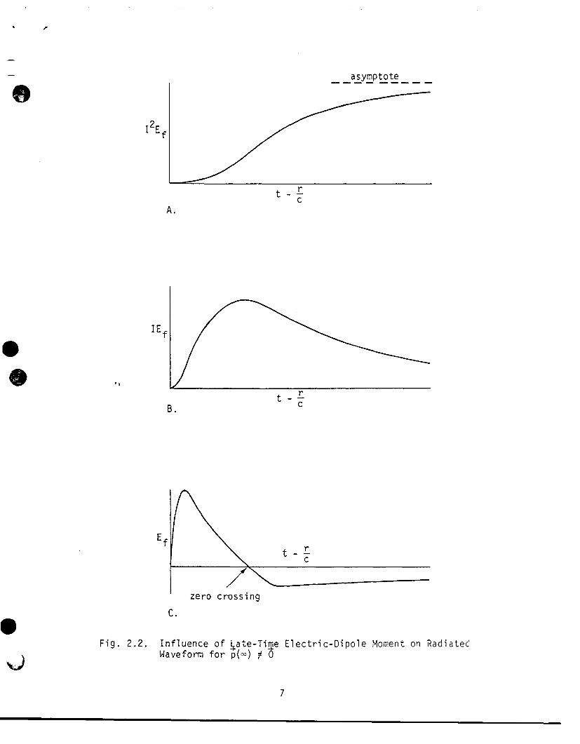
In time domain this concept of a non-zero ~(~) has imp~ications for the

radiated (far-field) temporal waveform. As shwn in [3] this property allows

the radiated temporal waveform to have one zero-crossing instead of the mini-

mum of two zero crossings required if~(~) = 8. To illustrate this consider-

the example in fig. 2.2. Here powers of I indicate repeated integrals with

respect to time and correspond to repeated multiplications by 1/s in complex-

frequency domain. Noting that o jsr-—

ff(;,s) + - ~ + Yt ● F(m) ass+O (2.5).

then multiplication by s‘2 gives’12Ef in time dcmain of the general form in

fig. 2.2A which rises smoothly (by our choice) from zero to a late-time value

governed by~(m) (per the Tauberian theorems of the Laplace transform).

Successive differentiation gives no zero crossing in fig. 2.2B and one zero

crossing in fig. 2.2C, the minimum number of zero crossings for the radiated

field. If the waveform in fig. 2.2A were allowed to go back to zero then at

least two zero crossings would appear in the radiated waveform. Here ~(t) has

been assumed to have a time-independent direction.

Note that the late-time dipole moment is computed from

6

●

6!9

%J

asymptoteI —--- —--- —

12Ef

t-;

A.

IEf

B.

‘f“t-:

/\I zero crossing

c.

Fig. 2.2. Influence of ~ate-TWaveform for p(L=)# 8

e Electric-Dipole Moment on Radiated

7

. .

(2.6)

~ = Cavm = late-time charge on simulator

ieq = equivalent length or mean charge separation distance

Pm(T’) = late-time charge density

Ca = simulator capacitance

[1

c -1Vm= Vol+: = late time voltage on simulator

!I

V. = charge voltage (if Marx generator then when fully erected)of capacitive pulser

Cg = pulser capacitance (if Marx generator then when fully erected)

Combining these gives

H

-1~(m)= vocal+> K

9eq

(2.7)

to

(or

or oby

From this we can see how to maxjmizefi(~). Note that~eq is proportional

the antenna length and Ca is proportional to the antenna length and width

fatness, but logarithmically in the latter case). Clearly antenna length

height is a matter of primary concern. The pulse generator can also help

large V. and large Cg, although increasing Cg too much beyond Ca is not useful.

Having first considered the design constraints for optimum low-frequency

perfor?nancelet us turn to the high-frequency aspects of the design, noting

that the latter should not be chosen in a form which significantly degrades

the former. Fortunately a circular conical geometry is appropriate to this

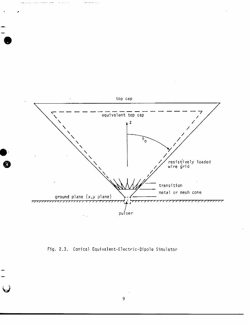
task. As illustrated in fig. 2.3we have the general concept of a typical

equivalent electric dipole. Note that this type of structure is analyzable by

image theory. The equivalent dipole moment (for produc{ng fields in the upper

half space) includes the image in its definition; the equivalent voltage is

twice the actual voltage on the cone and the equivalent capacitance is half

the actual capacitance. Note that a cone has the property of being “fat” at

the furthest distance from the ground plane, thereby enhancing the equivalent

height. The equivalent height is further enhanced by including a top cap on

the cone (of physical height h). The capacitance is enhanced by making the

cone fat (i.e., a “large” value of O.).

8

. . ...—

, .

top cap

——— .——

0“69

\

\

\\

\\

\

\

transition

metal or mesh cone

7///(/.///////{/{ /// / /.

/ / / / ///

‘“? “’’’’’’’’’’’’’’’’’’’’’’’’’’”

)J

pulser

Fig. 2.3. Conical Equivalent-Electric-Dipole Simulator

9

. .

. .

Near the cone apex some care is taken to make the geometry a good

approximation to a metal cone. At early times (or high frequencies) the

impedance is [2,4,5] ~

zeq = 2za= Zofg = Zm

f9 [1=+Rncot (>)

Z. =r

‘o~ (wave impedance)

Za ~ antenna impedance

(2.8)

Typical values of Za are 60 !2or 75 $2. The corresponding early-time fields are

I“-1

EO(t[ If

- ~) = Veq(t) 2r sin(e) Ln cot(~){

,,

‘Pemrf for 90 < e < Tr/2

..Y 9

veq(~)= Zva(t). . .

yam5 antenna’voltage

(2.9)

These results are determined primarily by the simulator geometry near the cone.,apex where one should be careful to maintain the cone geometry to a high degree

of approximation to ‘support the ideal high-frequency behavior.

- ‘For’iiitei?nediatefrequencies or times (wavelengths of the order of the

antenna height h) the antenna should be damped so as to make the radiated

field non resonant (natural frequencies for s + O have .Re[s] << -lIm[s]l)

creating a smooth spectrum for s = j~. This can be accomplished quite well by

use of a resistive loading on the antenna [5]

‘m[1-N’R’(E) = ~

= resistance per unit length along antenna(2.10)

E = arc parameter (meters) measured from cone apex alongantenna “surface”

o‘J

h’ s slant length of antenna, perhaps including radius of “top cap”

10

●4!9

—

—

This gives an input impedance

q(s) [1=2ia(s)=++z. =zm++l

aeq

Shl = Sth,

cth, = Zmca = Zm+

eq

Ca : antenna capacitance

which is conveniently just the series combination of a resistance and a

capacitance.

Including an equivalent generator capacitance and initial voltage

c ACgeq

‘Zg

v = 2V0‘eq

the radiated far-field waveforincan be calculated to give [5]

[[

-13Th , -aT ~ ,

Ne>t)=qJ- pco~e- l-e1u(Th,)

a[l - COS(9)]2

a

(2.11)

(2.12)

-a[Th,-[l-coS(e)]]•~l-e u(Th, - [1 - Cos(e)l)a [1 - cos(e)]2

[

-a~ ,h -aTh,1

+ 1 : COS(Q) - [l ; :os(e)121u(Thl)

-a[Th,-[l+c(js(e)]]+~i - e - ‘(Thl - [1 + Cos(e)])a [1 + cos(e)]2 I (2.13)

1 +Ca—=

C91 +

Ca3

c9eq

-rI=et-r

h h ‘(retarded time at observer)

i),L.

11

-.

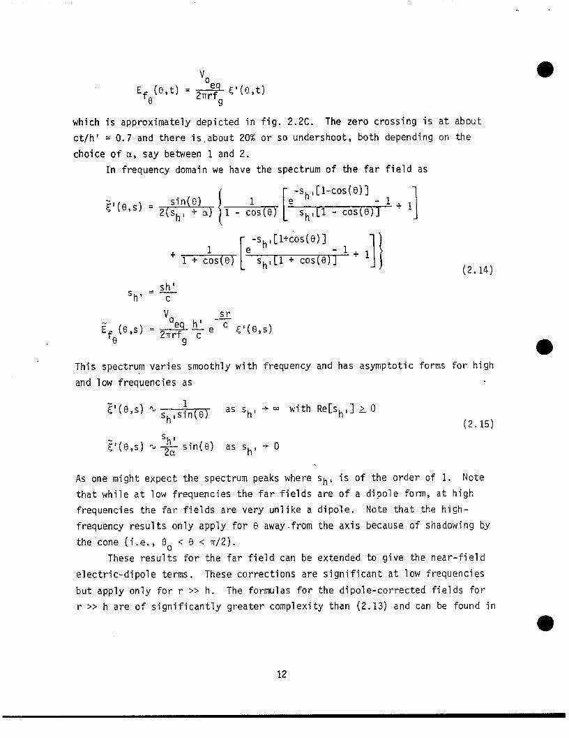
which is approximately depicted in fig. 2.2C. The zero crossing is at about

et/h’ = 0.7 and there is.about 20% or so undershoot, both depending on the

choice of a, say between 1 and 2.

In frequency domain we have the spectrum of the far field

7+i’(6,s) s sin(6[

e-’@c0s(e)3-1 ~ ~

2sh, +cl h“ sh, Ll - COS(6)-J

1

J

e-sh’[l+cO’(e)] -1 + ~+ 1 + ~os(fj sh,Ll + COS(~) 1 II

sh ‘s,=—hc

v sr-—‘eif (6,s) =~~e c g’(6,s)

9 9

as

(2.14)

This spectrum varfes smoothly with frequency and has asymptotic forms for high

and low frequencies as

“(6’S)‘* as‘h’ ‘o ‘ith‘ers+o(2,15)

;’(9,s) %* sin(B) as sh, + O

AS one might expect the spectrum peaks where sh, is of the order of 1. Note

that while at low frequencies the far fields are of a dipole form, at high

frequencies the far fields are very unlike a dipole. Note that the high-

frequency results only apply for B away-from the axis because of shadowing by

the cone (i.e., 00 < 3 < iT/2).

These results for the far field can be extended to give the near-field

electric-dipole terms. These corrections are significant at low frequencies

but apply only for r >> h. The formulas for the dipole-corrected fields for

r >> h are of significantly greater complexity than (2.13) and can be found in

12

–———=--———. -—

. m

—[14]. For r >> h estimates of E()and H+ can be obtained from transmission-

line approximations for the voltage and current along the cone using the

results of [5]. Note that at sufficiently early time (2.13) must be corrected

to give a non-zero rise time associated with the characteristics of the pulse

generator. This rise is often modelled by an inductance (switch inductance)

in series with the high-frequency antenna impedance Zm/2. In frequency domain

(2.14) can be corrected at sufficiently high frequencies to account for the

same phenomenon.

In the practical realization of a large EMP simulator of this type there

are introduced design features for reducing cost, weight, and wind loading.

One needs to be careful to preserve electromagnetic performance. In particular,

it is desirable to replace the ideal continuously resistively loaded circular

cone (and top cap) by a grid of wires with typically a set of lumped resistors.

The resulting wire grid or cage can be approximately treated by considering a

position for an equivalent conducting sheet (circular cone and top cap) which

is “behind” (away from the external fields) a distance of the rough order of

the wire spacing [1,4,11,16,17]. This implies that the wire cage should be

placed outside the ideal cone on 9 = 80 to some 6 > 60 as indicated in fig. 2.3.

One also should pay some attention to the transition from the metal cone

leaving the pulser to the wire cage structure. As indicated in fig. 2.3 one

can use triangular tapers of metal sheet or mesh to accomplish this purpose.

By making the length of this transition of the order of the local wire spacing

in the subsequent grid one can reduce any high-frequency (or early-time)

reflections of the wave propagation from the pulser along the metal (or dense-

mesh) cone to the sparse wire-grid cone [16].

●

d13

111, Hybrid EMP Simulator

There is a general class of EMP simulators which are by nature hybrids,

combining several electromagnetic concepts. These are defined by the follow-

ing three characteristics [15 section 2D].

“l) The early-time (high-frequency) portion of the wavefo~m reaching

the system is radiated from a relatively small source region compared to the

major simulator dimensions.

2) The low-frequency portions of the waveform are associated with

currents and charges distributed over the major dimensions of the simulator

structure. This structure either surrounds the system or is very close to it.

3) The structure is sparse so that most of the high-frequency energy

. radiates out of the simulator without reflecting off the simulator structure.

The structure is also impedance loaded’(including resistance) to further

reduce unwanted reflections in the simulator. This also dampens oscillations

in the intermediate frequency regjon where the simulator dimensions are com-

parable to.an appropriate fraction of a wavelength. At low frequencies the

structure reflection should become larger smoothly to make the fields transi-,.tion over to the static field distribution smoothly.” @

Thus a hybrid simulator is in general rather complex electromagnetically. The

fields of concern are’not described by a simple formula characteristic of, say

an electric or magnetic dipole, which contradicts these conditions [19].

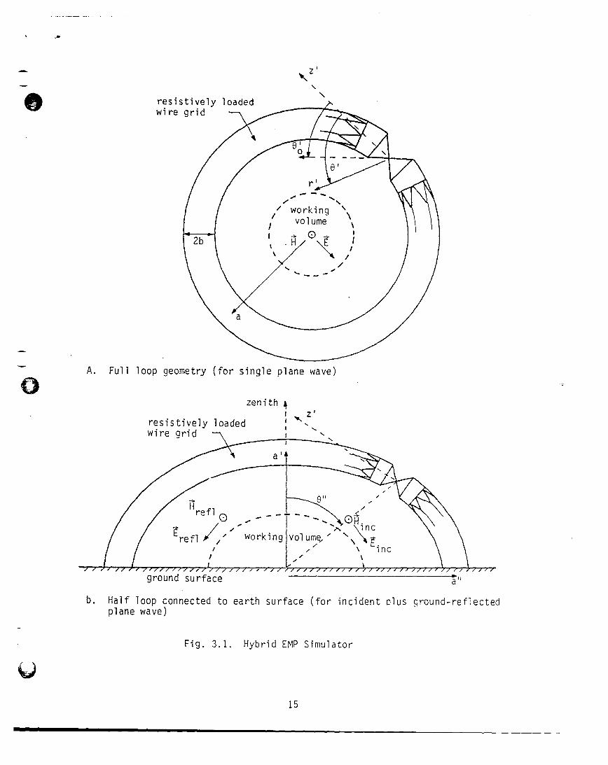
Figure 3.1 illustrates the general concept of a hybrid EMP simulator.

In fig. 3.1A there is a full loop, while in fig. 3.15 there is a half loop

connected to the earth (or sea water, etc.) surface. While a “full” hybrid

is not typically used (to generate an approximate single plane wave) because

of its relative inefficiency (field over the central working volume per pulser

volt) as compared with a parallel-plate type of simulator, it is useful for

understanding the performance characteristics of both kinds of hybrids. A

“half” hybrid which purposefully Includes the ground-reflected wave in tie

design can be approximately related to the “full” hybrid by image theory,

including images of both the antenna and pulser.

The early-time (and generally high-frequency) behavior is controlled by

the pulser and those portions of the simulator proper in the immediate vicinity

14

,.

k.z’\

—

A. Ful1

\resistively loadedwire grid

--~// -,/- working j-\// volume \ \\\\

loop geometry (for single plane wave)

zenith 4I I

resistively loaded I %,2I

wire grid<

I \1

\a’b

,.~11 /

/

(3 */~-”- “---- .* ah:

1

Incworking volume,H ‘i

/ , Fine//L / \

/ / // # \// </ /./// ////// ///// // /// / //////// // / ////// //// //// ///{7ground surface *

a”

b. Half loop connected to earth surface (for incident OIUS qround-reflectedplane wave)

—

— Fig. 3.1. Hybrid EMP Simulator

15

of the pulser as can be seen from speed-of-light considerations. Typically,

the pulser is configured to lie inside one or both cones of a circular bicone

so as to launch a spherical wave on the bicone from near its apex. As SUCh

some of the results of the previous section are also applicable here in terms

of the “equivalent” parameters (subscript ‘Ieq”)because of the full bicone.

As in fig. 3.1, using primed coordinates centered on the bicone with the z’

axis as the bicone axis we have

Za=zm=zfOg

Va(t)EO,(t -;) = **rlfg for 0~ < e’ < m-e:

(3.1)

This result is limited by what is referred to as “clear time” which is the

time between the first arrival of the wave from the cone apex and the arrival

of the wave from the first discontinuity where the bicone is truncated and a

transition”to the remainder of the simulator proper (typically a resistively

loaded wire cage) is begun [2]. Note that the maximum clear time is along

6’ = n/2, and that the clear time diminishes to zero at 6’ = B: and 0’ = T-6:.

In particular the clear time should be larger than the rise time of the wave-

form applied by the pulser to the bicone a~ex if one wishes to radiate the

“peak” of the waveform before encountering the clear-time limitat~on. This

advantage in having a large clear time also helps the high-f~quency content

of the resulting waveform.

This transition is similar to that discussed in the previous section

except that the transition leads to a cylindrical wire cage instead of an

approximate conical one. In this case the metal sheet or dense mesh cones can

first transition to circular cylinders (of similar material) of a length of

the order of the cone radius at the transition. This is followed by triangular

tapers of a similar length leading to the wires of the cage. Thjs transition

is important so that large reflections are avoided or minimized at the discon-

tinuity in the direction and density (sheet versus wire cage) of the simulator

conductors. This is especially helpful at the higher frequencies, Note that

16

. .

—

—

—

.

—

the effective radius of the wire cage (as an equivalent cylinder) can be

computed from [4] as

~r l/N

()!?% Qbl bl

N : number of wires in cage

bl = cage radius

beq = equivalent cylinder radius

ro = wire radius

Cross-connecting conductors (hoops) are typical

(3.2)

ly used to keep the local poten-

tial differences between the wires minimal. Resonances are avoided in the

resulting loops by the presence of series resistors in the wires which also

give tie desired resistive loading in the simulator proper.

Turning to the low frequencies (A >> a) let us distinguish the two cases

of hybrids by a superscript “l” for the full loop giving an approximate single

plane wave as in fig. 3.1A, and by a superscript “2” for the half loop con-

nected to the earth surface giving two approximate plane waves as in fig. 3.lB.

While at high frequencies the two waves are quite separable due to transit

times making (3.1) applicable to both types of hybrids, at low frequencies a

measurement of the electromagnetic fields of necessity includes all waves

present.

Consider first the low-frequency magnetic field. In the full loop geom-

etry of fig. 3.1A let the loop be circular (a toroid) with major radius a and

minor radius b. Then relating the low-frequency magnetic field in the center

to the low-frequency current by [6,8,9]

V.= open circuit voltage of capacitive generator(charge voltage)

(3.3)Qg = generator charge

This low frequency magnetic field has the relation to the time domain waveform

as its integral or “area”, i.e.,

17

(3.4)H(l)(0) = ~ H(t) dt.W

Given some specified waveform then the required generator charge can be com-

puted. If V. is known (say specified frcm (3.1)) then Cg is also dete~ined.

For the half loop connected to the ground surface, hcwever, we have

the factor of 2 accounting for the ground reflection of an incident plane wave,

the reflection coefficient of the tangential magnetic field being 1,0 at low

frequencies, Then using

(3.6)

the specification of the incident plane wave can be used to determine the

generator capacitance. Note that as a practical matter the half loop is not

‘normally circular; a good design has it made elliptical with minor radius a’

‘“andmajor radius a“. This is related to the practical mechanical problem of

realizing a large a’ (height); a“ (half length on the ground) is much easier

to make large. In this case we take

a s avg(a’,a”) (3.7)

where the average can be of many kinds. Typically this average is chosen to

make the loop area or the loop circumference the same as a loop of radius a.

Next consi”derthe low-frequency electric field. The-full loop is simpler

to analyze. If the loop is resistively loaded then at low frequencies there

is an electric potential (quasistatic) associated with the electric field along

the loop structure given by 112,13]

Etan = i(o)R’

R’ = resistance per unit length along loop

This field establishes a potential which extends through space,

through the working volume in’the center of the loop (simulator

18

(3.8)

in particular

proper).

(3.14)

This half-loop resistance is typically 500$2 or a little more.

For intermediate frequencies (A/a of the order of 1 or somewhat less)

the situation is more complicated. Detailed calculations [12,131 indicate

that the desired ratio of electric and magnetic fields near the center as in

(3.10) ismaintajned typically to within about 40% or so of this ideal value

across this intermediate frequency band. This shows the non-resonant charac-

ter of this idealized hybrid simulator associated with radiation “losses” and

resistive loading.

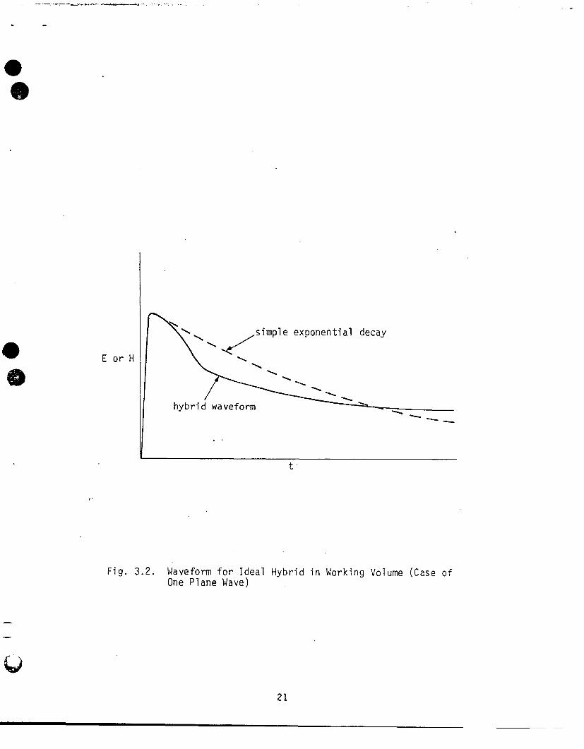
In transitioning from the high-frequency to a low-frequency behavior

note that the impedance driven by the pulser increases significantly from that

given by (3.1) (say 120 ilor 150 !3)at high frequencies to that given by (3.11)

or (3.14) (say 1 kQ or 500 Q) at low frequencies. This makes the decay of the

transient waveform not a simple exponential. As illustrated in fig. 3.2 the

waveform initially decays rapidly but then flattens out; this is compared to

a simple exponential decay with the same “area” (constrained by the pulser

““charge-asin (3.3) or (3.6)). This example is taken for the single approxi-

mate plane wave of a full loop because of its relative simplicity. The case

of two plane waves with a half loop gives a purposely more complex waveform,

varying with position near the “center”, which also occurs with the interfer-

ence of two plane waves.

If the observer nwves off the plane of the loop then other polarizations

of the incident (first) plane wave become possible. On the plane of the loop

the polarization is TMwith respect to the vertical. However, TE polarization

is achievable by placing the pulser at the top of the arch in fig. 3,18

(6” = O) and moving ~he observer along (or above) the ground (or near the loop

axis). One should not go too far off the plane of the loop; the performance

of this type of simulator is in part related to the near fields. Furthermore,

TE polarization at angles of incidence near grazifigto the ground significantly

reduces the resultant EM fields (including ground reflection) at the observer

(i.e., the system under test) thereby typically significantly reducing the

interaction with the system; this is then typically a case of minimal interest.

20

-—-.-ka/---- -~ee . .

.

Eor H

+

simple exponential decay

\hybrid waveform \ - <

---

. .

t

..

Fig. 3.2. Waveform for Ideal Hybrid in Working Volume (Case ofOne Plane Wave)

21

Circular or elliptical hybrids are not the only possible geometries,

although these geometries do have some significant performance advantages.

For example, another hybrid geometry has a cylinder (wire cage) divided by

the pulser (effectively 8“ = O) with distant terminations from the cylinder

to the ground at both ends [7]. However, beyond some point arbitrarily

increasing the length of the simulator along the ground surface does not

improve the fields in the working vo?ume.

.

22

.- ..

. ,&

●49 IV. summary

These two important types of high-altitude EMP simulators are becoming

widely used for their appropriate simulation roles. Both have their own opti-

mization conditions and trade-offs which should be considered in designing

such simulators for specific intended applications.

!“.”

●a!)

—

%&).4

23

References

1.

2.

3.

4.

5.

6.

7.

8.

9.

10.

11.

12.

13.

C. E. Baum, Impedances and Field Distributions for Parallel PlateTransmission Line Simulators, Sensor and Simulation Note 21, June 1966.

C. E. Baum, A Circular Conical Antenna Simulator, Sensor and SimulationNote 36, March 1967.

C. E. Baum, Some Limiting Low-Frequency Characteristics of a Pulse-Radjating Antenna, Sensor and Simulation Note 65, October 1968.

C. E. Baum, Design of a Pulse-Radiating Dipole Antenna as Related toHigh-Frequency and Low-Frequency Limits, Sensor and Simulation Note 69,January 1969.

C. E. Baum, Resistively Loaded Radiating Dipole Based on a Transmission-Line Model for the Antenna, Sensor and Simulation Note 81, April 1969.

C. E. Baum, Some Considerations Concerning a Simulator with the Geometryof a Half Toroid Joined to a Ground or water Surface, Sensor and Simula-tion Note 94, November 1!369.

C. E. Baum, Some Considerations Concerning a Simulator with the Geometryof a Cylinder Parallel to and Close to a Ground or Water Surface, Sensorand Simulation Note 97, January 1970.

C. E. Baum, Low-Frequency Magnetic Field Distribution for a Simulatorwith the Geometry of a Half Toroid Joined to the Surface of a Mediumwith Infinite Conductivity, Sensor and Simulation Note 112, July 1970.

A. D. Yarvatsis and M. I. Sancer, Low-Frequency Magnetic Field Distribu-tion of a Half Toroid Simulator Joined to a Finitely Conducting Ground:Simple Ground Connections, Sensor and Simulation Note 122, February 1971.

C. E. Baum, Some Characteristics of Electric and Magnetic Dipole Antennasfor Radiating Transient Pulses, Sensor and Simulation Note 125, January1971.

D. F. Higgins, The Effects of Constructing a Conical Antenna Above aGround Plane Out of a Number of Thin Wires, Sensor and Simulation Note142, January 1972.

C. E. Baum and H. Chang, Fields at’the Center of a Full Circular TORUS ~and a Vertically Oriented TORUS on a Perfectly Conducting Earth, Sensorand Simulation Note 160, December 1972.

H. Chang, Electromagnetic Fields Near the Center of TORUS, Part 1: Fieldson the Plane of TORUS, Sensor and Simulation Note 181, August 1973.

24

4./9

14. B. K. Singaraju and C. E. Baum, A Simple Technique for Obtaining theNear Fields of Electric Dipole Antennas from Their Far Fields, Sensorand Simulation Note 213, March 1976.

15. C. E. Baum, EMP Simulators for Various Types of Nuclear EMP Environments:An Interim Categorization, Sensor and Simulation Note 240, January 1978;also as IEEE Trans. Antennas and Propagation, January 1978, pp. 35-53,and IEEE Trans. EM, February 1978, pp. 35-53.

16. W. S. Kehrer and C. E. Baum, Electromagnetic Design Parameters forATHAM4S II, ATHAMAS Memo 4, May 1975.

17, C. E. Baum, J. E. Partak, J. E. Swanekamp, and T. Dana, ElectromagneticDesign Parameters for NAVES II, NAVES Memo 1, March 1977.

18. K.S.H. Lee (cd.), EMP Interaction: Principles, Techniques, and ReferenceData, EMP Interaction 2-1, December 1980.

19. J. D. Jackson, Classical Electrodynamics, Wiley, 1962.

. .

m

—

—

25