abstract - Universidade Estadual de Maringá

Bol. Soc. Paran. Mat. (3s.) v. 39 4 (2021): 35–55.c©SPM –ISSN-2175-1188 on line ISSN-00378712 in press

SPM: www.spm.uem.br/bspm doi:10.5269/bspm.40837

Efficient Procedure to Generate Generalized Gaussian Noise Using

Linear Spline Tools

A. Monir, H. Mraoui and A. El Hilali

abstract: In this paper, we propose a simple method to generate generalizedGaussian noises using the inverse transform of cumulative distribution. This in-verse is expressible by means of the inverse incomplete Gamma function. Since theimplementation of Newton’s method is rather simple, for approximating inverse in-complete Gamma function, we propose a better and new initial value exploiting theclose relationship between the incomplete Gamma function and its piecewise linearinterpolant. The numerical results highlight that the proposed method simulateswell the univariate and bivariate generalized Gaussian noises.

Key Words:Generalized Gaussian noise, Incomplete Gamma function ratios,Weakly singular integrals, Inversion of incomplete Gamma functions, Linear splineinterpolation.

Contents

1 Introduction 36

2 Elliptical Distributions 38

2.1 Simulation of elliptical distributions . . . . . . . . . . . . . . . . . . 39

2.2 Description of some elliptical distributions . . . . . . . . . . . . . . . 39

2.2.1 Multivariate Gaussian distribution . . . . . . . . . . . . . . . 40

2.2.2 Multivariate Generalized Gaussian distribution. . . . . . . . . 40

3 Numerical evaluation of the incomplete Gamma function 43

4 Inversion approximations for incomplete Gamma function 46

4.1 Asymptotic expansions for P−1(a, p) as p→ 1− . . . . . . . . . . . . 47

4.2 Approximation for P−1(a, p) on [0, 1− ǫ]. . . . . . . . . . . . . . . . 47

5 Applications 49

5.1 Simulating of univariate generalized Gaussian noise . . . . . . . . . . 49

5.2 Simulation of bivariate generalized Gaussian noise . . . . . . . . . . 51

6 Conclusion and discussion 53

2010 Mathematics Subject Classification: 65D07, 65D17, 41A15, 41A28, 65D05.

Submitted December 04, 2017. Published May 28, 2018

35Typeset by B

SPM

style.c© Soc. Paran. de Mat.

www.spm.uem.br/bspm

http://dx.doi.org/10.5269/bspm.40837

36 A. Monir, H. Mraoui and A. El Hilali

1. Introduction

The study and application of univariate and multivariate generalized Gaussiandistributions (GGD) is an active field of research in theoretical and applied statis-tics. This class of processes has merited considerable attention by many scientistsfor two fundamental reasons: firstly, because it captures the observed heavy tails;secondly, because the probability density characterizes this class has fully paramet-ric form. Recently, GGD have been widely adopted in modeling various physicalphenomena [3,4,19,21]. As known, the generation of multivariate distributions hasnot been investigated extensively and we have not enough literature on Monte Carlotechniques for synthesizing multivariate random processes, except from the workdone by Johnson [14]. Recently, new initiatives designed to target this area of re-search in order to better understand and control the multivariate random processes[6,23]. It is obvious that there is no universal method for simulating a random vari-able or random vector from known distributions with Monte Carlo methods for thestudy of the behavior of statistics with unknown sampling distribution. In general,the generation of multivariate distributions is more complicated to implement, be-cause the usual method based on the inverse of the cumulative distribution functionused with univariate distributions can not be applied. An option to circumvent theproblem of generation multivariate random is to use multivariate extensions of gen-eration methods for univariate random variable such as ratio-of-uniforms method,acceptance-rejection (AR) methods or transformation method. An other way, inmultidimensional approach leads to generating random variates, is to use the con-ditional distribution method [14]. These current standards methods of simulatingmentioned before suffer from limitations and become hopelessly inefficient whenapplied to realizations of stochastic multidimensional processes see. [23]. When thecomputation of the conditional distribution is difficult, a transformation of vectorcan probably be considered. However, for several multivariate distributions, it ishard to define transformations of random vectors from which samples can be easilyobtained.

In this contribution, we introduce the multivariate generalized Gaussian dis-tribution which is a special case of the larger class of elliptical distributions. Forthe sake of simplicity we deal with one and two dimensions, but the results canbe easily extended to higher dimensions. We present so computational algorithmto generate univariate and bivariate generalized Gaussian distribution using trans-formation approach. Gomez, Gomez-Villegas and Marın [13] have proved that thegeneration of multivariate generalized gaussian by using polar coordinates is veryeasy, if we can simulate sequences from Gamma distribution. We are going to useclassical Monte carlo procedure to simulate sampling from Gamma distribution. Inthis case, we should invert incomplete Gamma function. This special function hasno elementary inverse of its argument, hence requiring numerical evaluation to beperformed to obtain an approximation of this function.

The regularized upper and lower incomplete Gamma functions are defined by

Efficient Procedure to Generate Generalized Gaussian Noise 37

the integrals [20]

Q(a, x) =1

Γ(a)

∫ ∞

x

ta−1 exp(−t)dt,

P (a, x) = 1−Q(a, x) =1

Γ(a)

∫ x

0

ta−1 exp(−t)dt,

where we assume that a > 0 and x ≥ 0, and Γ(a) =∫∞

0 ta−1 exp(−t)dt is the well-known Gamma function. The problem of inverting functions Q(a, x) and P (a, x)is one of the central problems in statistical analysis and applied probability, withvarious applications [8,2].

However, it is difficult to compute the inverse P−1(a, ·) of the function P (a, ·)because its shape depend on the parameter a in a significant way. Several ap-proaches are available in the literature for computing P−1(a, ·). One possibility isto use the Newton methods to computing x when p = P (a, x) is given, see [7,12].However, this approach has some practical difficulties. If the initial value is notgood enough, the method might diverge. This leads to the question of how to finda good starting value, which is tricky in itself. More recently, in [12], the analyticalapproach from earlier literature is summarized and new initial estimates are de-rived for starting the fourth order Newton method. This method is not, however,as flexible as is desirable because the starting values need: dividing the domain ofcomputation, Taylor expansion, continued fraction, uniform asymptotic expansion,asymptotic inversion, inversion of the complementary error function. On the otherhand, it is rare to use fourth and higher-order formulas in solving a single nonlinearequation in practical computations, see Section 9.4 of [22].

Furthermore, in the present case, the functions P (a, ·) and whose derivativesmay have singularities near the endpoint 0 for some values of a. As an alterna-tive, we take care of the first point by starting from a sufficiently precise solutionprepared by the piecewise linear interpolant of P (a, ·) with special graded grids.Computational experience indicates that at few iterations of Newton method aresufficient to achieve the double-precision solution in a reasonable time frame.

On the other hand, the numerical inversion techniques require evaluation of theincomplete Gamma function P (a, x). As explained in Chapter 5 of [11], numericalquadratures can be an important tool for evaluating special functions. In particular,when selecting suitable integral representations for these functions. In this paper,we show that the numerical quadratures for weakly singular integrals by nonlin-ear spline approximations proposed in [15], is particularly efficient for computingnumerically P (a, x). Theoretical results and numerical experiments indicate thatthese methods perform adequately when the Gamma probability density functionis smooth or has weak singularities.

The main advantage of the proposed numerical procedure, to evaluate the in-complete Gamma function and its inverse, is that is very simple to implement anddoes not require any elaborate special mathematical functions software, and canbe straightforwardly coded in any programming language with standard algebra.

The contents of this paper is as follows. Section 2 introduces the definition


of Generalized Elliptical Distributions, with presentation of the most famous ex-amples. We also give the procedures for synthesizing univariate and bivariategeneralized Gaussian processes. In Section 3, we apply the Gauss-Legendre-typequadrature to compute the incomplete Gamma function ratios for positive values ofa and x. The procedure for computing x when a and P (a, x) are given is describedin Section 4. Simulations for univariate and bivariate generalized Gaussian areprovided and results are interpreted in Section 5. Section 6 concludes the paper.

2. Elliptical Distributions

As known multivariate normal distribution has enjoyed a significant role inmany practical applications such as in behavioral and social sciences, biometrics,econometrics, environmental sciences, and finance. Real data are often not nor-mally distributed in behavioral sciences, especially when the tails are thicker orthinner than those of normal distributions. The nonnormal distributions werechosen because they were thought to be realistic representations of distributionsencountered in the behavioral sciences. Many alternative methods exists when thenormality assumption is not justifiable. One choice is the elliptical family of dis-tributions which include the normal one and share many of its flexible properties.This class of distributions has received an increasing attention in the statisticalliterature, particularly due to the fact of including important distributions as, forexample, Student-t, Generalized Gaussian, Logistic, Laplace, among others, withheavier or lighter tails than the normal one. This class of distributions was in-troduced by Kelker [16] and was widely discussed in Fang, et al. [9]. Ellipticaldistributions are very often used, particulary in risk and financial mathematics[24].

The random vector X = (X1, X2, . . . , Xp)T is said to have an elliptical dis-

tribution with parameters vector ν(p × 1) and definite positive symmetric matrixΛ(p× p), if its characteristic function can be expressed as

E[exp(itTX)] = exp(itT ν) Φ(tTΛ t), (2.1)

for some scalar function Φ called characteristic generator of X , and where tT =(t1, t2, · · · , tn). It should be mentioned that, in general, the elliptical distributionrandom vector doesn’t necessarily have a density, but in this work we will consider aclass of elliptical distribution having an analytic expression of density. This densityfunction is given by ( see. Fang et al. [10, p. 35])

f(x; Λ, ν) =1√

det(Λ)g([

(x− ν)TΛ−1(x− ν)])

, (2.2)

g(.) called density generator. Where,

• Λ is positive definite;

• g(.) ≥ 0, with∫ +∞

−∞

∫ +∞

−∞· · ·

∫ +∞

−∞g(yT y)dy1dy2 · · · dyp = 1.


If X has this distribution and Y = L−1(X − ν), where LLT = Λ, then Y hasprobability density function (abbr. pdf) g(yT y), spherically contoured.

A nice property of an elliptical distribution function is the fact that its multi-variate density function may be expressed via the density generator.

2.1. Simulation of elliptical distributions

Let (yp)T be an p-dimensional vector, every yi can be written in polar coordi-

nates as

y1 = r sin θ1

y2 = r cos θ1 sin θ2,

y3 = r cos θ1 cos θ2 sin θ3,

...

yp−1 = r cos θ1 cos θ2 · · · cos θp−2 sin θp−1,

yp = r cos θ1 cos θ2 · · · cos θp−2 cos θp−1

where,

• r ≥ 0;

• − 12π < θi ≤ 1

2π, 1 ≤ i < p− 1, and −π < θp−1 ≤ π.

The jacobian determinant form

J(r, θ) = rp−1[cos(θ1)]p−2[cos(θ2)]

p−3 · · · [cos(θp−3)]2 cos(θp−2)

If the pdf of Y is g(y′y), then the pdf of R, Θ is

J(r, θ)g(r2) = rp−1g(r2)[cos(θ1)]p−2[cos(θ2)]

p−3 · · · [cos(θp−3)]2 cos(θp−2).

R and Θ are independent, and the marginal pdf of R is

2πp2

Γ(p2 )× rp−1g(r2).

Note that 2πp2

Γ( p2 )

corresponds to the uniform density on the unit hypersphere.

2.2. Description of some elliptical distributions

In the next, we discuss two families of elliptical distributions: the normal whichis the most famous member of this family, and Generalized Gaussian distributionwhich is a general case of the normal distribution.


2.2.1. Multivariate Gaussian distribution. The Gaussian distribution, also callednormal, is a special case of the larger class of elliptical distributions with the densitygenerator g(t) = exp(−t/2). A random vector X = (X1, X2, . . . , Xp)

T follows amultivariate normal distribution, symbolically denoted by X ∼ Np(µ,Σ), then thejoint density of X is given by [13]

f(x; Σ, µ) =1√

2πdet(Σ)exp

(− 1/2

[(x− µ)TΣ−1(x− µ)

]). (2.3)

Synthesizing multivariate Normal data is relatively easy and fast. It has there-fore been used for many purposes and in vast number of applications. In manyapplications, however, the multivariate data that arise in practice are not well ap-proximated by a multivariate Gaussian distribution, especially when we have aheavy tail behavior.

2.2.2. Multivariate Generalized Gaussian distribution. An elliptical vector X issaid to have a multivariate Generalized Gaussian distribution if its density gener-ator can be expressed as g(t) = exp(−αtβ), for α, β > 0.

Let X = (X1, X2, . . . , Xp)T be an p-dimensional random vector distributed as

a multivariate generalized Gaussian distribution, if its probability density functionhas the form [21]

f(x; ΣX , β, α, µ) = ηp exp(−[α (x− µ)TΣ−1(x− µ)

]β), (2.4)

where α and β are two parameters which can represent the spherical shape of themodel and ηp indicates a normalized constant defined by α, β and the dispersionmatrix Σ, symmetric and positive definite.

Note however that the multivariate Gaussian pdf is recuperated by setting β = 1,we will call the distribution with β = 1/2 the multivariate Laplace distribution.If β < 1, the distribution (2.4) has heavier tails compared to the multivariateGaussian distribution.

If we suppose that the random quantity X has a zero-mean and identity ma-trix covariance, called in this case standard generalized Gaussian, the probabilitydensity function (2.4) will become

fX(x) := f(x; IX , β, α, 0) = η exp(−[α xTx

]β). (2.5)

We restrict our attention to these conditions knowing that arbitrarymean µ = E[X ]and covariance matrix ΣX = E[(X−µ)(X−µ)T ] can straightforwardly be restored

by the change of variable X ← LD12X + µ, where L is an orthogonal matrix such

that LTΣL = D, with D is the diagonal matrix of eigenvalues of Σ.We note that multivariate distributions with circular contours are a class of

distributions that are useful for modelling heavy tailed multivariate data. In [1],the case of circular contours defined by polar coordinates is analyzed including itssimulation procedure which is based on a rejection method to simulate a Gammarandom variable. However, the rejection method has some important limitations.


Another way of obtaining draws from some density of interest is to use the inversetransform method. This method is considered useful and effective, especially forsampling from univariate distributions. The method also preserves monotonicityand correlation. Further, with inversion method, small distribution parameterperturbations cause small changes in the produced variates. This effect is usefulfor sensitivity analysis. Contrast this to rejection method, see [17]. Mention mustbe made that some researchers avoid using this method for simulation, because formany distribution functions we do not have an explicit expression for the inverseof cumulative distribution function. We call numeric computation to resolve thisproblem.

For simplicity we will focus on the univariate and bivariate cases, but the resultscan be easily generalized to p dimensions.

Univariate case : The probability density function of generalized Gaussian noiseis defined as:

f(x) =α

2λΓ(1/α)exp

(−∣∣∣x

λ

∣∣∣α)

, (2.6)

for x ∈ R, α > 0 (shape parameter), and λ = (Γ(1/α)/Γ(3/α))1/2.

The cumulative distribution function (cdf) corresponding to (2.6) is (see, e.g.,Monir [18])

Fα(x) =

{12Q

(1α ,

(− x

λ

)α)for x ≤ 0 ,

1− 12Q

(1α ,

(xλ

)α)for x ≥ 0 .

(2.7)

It is well known that the inverse F−1α can be expressed in terms of Q−1 (inverse

of the regularized incomplete Gamma function), i.e.,

F−1α (u) =

{−λ

(Q−1

(1α , 2u

)) 1α , if 0 < u ≤ 1/2

λ(Q−1

(1α , 2(1− u)

)) 1α , if 1/2 < u ≤ 1.

(2.8)

Equation (2.8) solves the problem of synthesizing a generalized Gaussian noisewith shape parameter α from a uniform process, provided we are able to handlethe numerical evaluation of the function Q−1.

Bivariate case : We consider a random variable pair (X1, X2) distributed as 2Dgeneralized Gaussian, we can assume that the variables X1 and X2 are zero meanand uncorrelated. The joint probability density function is given by:

fX1,X2(x1, x2) =βΓ( 2β )

2πΓ2( 1β )σ2e−( Γ( 2

β)

2Γ( 1β

)

x21+x2

2σ2

)β

, (2.9)

where β > 0, and σ2 > 0.

Every x = (x1, x2)T can be written in polar coordinates as:

x1 = r sin(θ), x2 = r cos(θ).


Let X1 = R cos(Θ) and X2 = R sin(Θ), where R ≥ 0 and 0 ≤ Θ < 2π. Then, thejoint pdf in polar form is given by:

fR,Θ(r, θ) = rfX1,X2

(r cos(θ), r sin(θ)

)(2.10)

=βΓ( 2β )r

2πΓ2( 1β )σ2e−( Γ( 2

β)

2Γ( 1β

)

r2

σ2

)β

= fR × fΘ. (2.11)

By reassigning the parameters, the marginal pdf of R is obtained by fR(r) =2βr

α2Γ( 1β)e−(

rα )

2β

and the marginal pdf of Θ is obtained by fΘ(θ) =12π , where α =

σ

√2Γ( 1

β)

Γ( 2β).

It is clear that the variable Θ has a uniform distribution Θ ∼ U[0 2π], thesecond variable R follows generalized Gamma distribution R ∼ GG(α, 2, 2β). Thecumulative distribution function of R is

F (r) = P

(1

β,( r

α

)2β), (2.12)

where P (, ) is regularized lower incomplete gamma function.We want to invert F (r) of (2.12) and show that this inverse can be expressed

in terms of P−1(a, ·). We write for inversion under the equivalent form F =

P(

1β ,

(rα

)2β), which is invertible under the form r = α×

(P−1

(1β , F

)) 12β

, yielding

F−1(u) = α×(P−1

(1

β, u

)) 12β

. (2.13)

If we know how to evaluate P−1(a, ·), the equation (2.13) solves the problem ofsynthesizing variable R with marginal density fR from a uniform variable.

Once we have solved the equation(2.13), we can easily generate independentlypoints (X1, X2) from the joint standard generalized Gaussian distribution withshape parameter β as follows:

Algorithm 1.

1. Generate two independent random numbers U1 and U2 from U[0 1] distribu-tion.

2. Compute R = α×(P−1

(1β , U1

)) 12β

, and Θ = 2πU2.

3. Then set

X1 = R cos(Θ),

X2 = R sin(Θ).


This simulation scheme is particularly simple for the case of circular contoursand provides a general method for simulation of the resulting families with differentparameter shape values β.

Mention must be made that in both cases, we have to evaluate the inverse ofincomplete Gamma function. We now address this problem.

3. Numerical evaluation of the incomplete Gamma function

Let m be an integer. Note that the symbol Cm[0, d] denotes the set of allfunctions defined on [0, d] with values in R whose firstm derivatives are continuous.If there are no continuous derivatives we write C[0, d] = C0[0, d].

For α > −1 and nonnegative integer k, define Type(α, k, 0), see [15], as theset of all functions u ∈ Ck]0, d] such that

∣∣∣u(k)(x)∣∣∣ ≤ K |x|α−k

, x ∈]0, d].

The parameter α is called the index of singularity. The modulus of continuityof a function u ∈ C[0, d] is defined to be

ω[0,d] (u, δ) = sup {|u(x)− u(y)| : |x− y| ≤ δ} .

The collection of Holder continuous real-valued functions with exponent α isdenoted by Hα. We say u ∈ Hα if there is a constant M > 0 so that

ω[0,d] (u, δ) ≤Mδα, ∀ δ > 0.

We first rewrite P (a, x) as

I(fa)(x) :=

∫ x

0

fa(t)dt (3.1)

where the Gamma probability density function fa is given by

fa(x) =∂

∂xP (a, x) = xa−1 exp(−x)/Γ(a).

A classical and efficient technique for the numerical evaluation of integrals ofthe form (3.1), where fa is a smooth or nonsmooth function, is to approximate

I(fa)(x) by I(fa)(x) where fa is a spline approximant of fa, for which I(fa)(x)

can be easily calculated. In [15], the authors have considered the case where fa isthe (k − 1)th degree continuous piecewise Lagrangian interpolant of fa and theyhave studied the convergence order when fa is smooth or has weak singularities.A more detailed discussion of this quadrature can be found in [15].

For given integers n, k let

πa : t0 = 0, tj = jrn−rx, j = 1, . . . , n,


be a (strict) partition of the finite interval [0, x], where r ≥ 1 is a real numberwhich depends upon the index of singularity a. Set

S(−1)k−1 (πa) = {s : s|[tj,tj+1]

∈ Pk−1, 0 ≤ j ≤ n− 1},

where Pk−1 denotes the set of polynomials of degree not exceeding k − 1. Note

that the elements of S(−1)k−1 (πa) may have jump discontinuities at the interior points

of the grid πa.

Let ζl and wl, l = 1, . . . , k, be the Legendre-Gauss nodes and weights on theinterval [−1, 1] with truncation order k, respectively. In every sub-interval [tj , tj+1],j = 0, . . . , n− 1, we introduce k interpolation points tjl, l = 1, . . . , k:

tjl =

tj if ζ l = −1(tj + tj+1 + ζ l(tj+1 − tj))/2 if − 1 < ζ l < 1,tj+1 if ζ l = 1.

Given a function g ∈ C[0, x], we determine its piecewise polynomial interpolationfunction Pn,kg by formula

Pn,kg(t) =n−1∑

j=0

k∑

l=1

g(tjl)Ljl(t), t ∈ [0, x],

where

Ljl(t) =

m=k∏

m=1,m 6=l

t− tjmtjl − tjm

if t ∈ [tj , tj+1],

0 otherwise.

Now setting α = a − 1. If 0 < a < 1, then for any integer k we have fa ∈Type(α, 2k, 0), see [15]. Since −1 < α < 0, implies that fa is unbounded at 0.

Define a piecewise polynomial fa,n,k over [0, x] with πa by

fa,n,k(t) =

{0, if t ∈ [t0, t1],Pn,kfa(t), if t ∈ [t1, tn].

Then, we use I(fa,n,k)(x) to approximate I(fa)(x), where

I(fa,n,k)(x) =

n−1∑

i=1

ti+1 − ti2

k∑

l=1

wlfa

(ti+1 − ti

2ζ l +

ti+1 + ti2

). (3.2)

Let r = 2k1+1a with k1 ≤ k. By applying Theorem 3.1 of [15], we have the

following result concerning the accuracy of the Gauss-Legendre-type quadraturescheme

|I(fa)(x)− I(fa,n,k)(x)| = O(n−2k1

).


If a > 1, for any integer k we have fa ∈ Type(α, 2k, 0), see [15]. Furthermore,since α > 0 it follows that fa is an α-Holder continuous function. In this case,define a piecewise polynomial fa,n,k over [0, x] with knots πa by the following rule:

fa,n,k(t) =

{fa(t1)

tt1, if t ∈ [t0, t1],

Pn,kfa(t), if t ∈ [t1, tn].

Hence, I(fa)(x) is now approximated by

I(fa,n,k

)(x) = ta1 exp(−t1)/(2Γ(a)) +

n−1∑

i=1

ti+1 − ti2

k∑

l=1

wlfa

(ti+1 − ti

2ζ l +

ti+1 + ti2

).

If r = 2k1/α with k1 ≤ k. In this case, we have

|I(fa)(x)− I(fa,n,k

)(x)| = O

(n−2k1+1

).

Finally, if a > 2k+1 or a is a nonnegative integer then fa ∈ C2k[0, x]. Moreover,we use the classical composite Gauss numerical integration scheme to approximateP (a, x)

I(fa)(x) ≈ I (Pn,kfa) (x) =

n−1∑

i=0

ti+1 − ti2

k∑

l=1

wlfa

(ti+1 − ti

2ζ l +

ti+1 + ti2

),

with r = 1. In this case we have |I(fa)(x) − I (Pn,kfa) (x)| = O(n−2k+1

).

Remark 3.1. 1. For large values of a and t, say a ∼ t, fa(t) may be computableusing Stirling’s formula for the Gamma function see [12]. Write fa(t) in theform (see [12])

fa+1(t) =e−

12aη

2

√2πaΓ∗(a)

, where Γ∗(a) =Γ(a)√

2π/aaae−a,

and 12aη

2 = β− 1− ln(β), β = t/a. When a −→ +∞, the function Γ∗(a) hasthe well known asymptotic expansion [25, p. 253]

Γ∗(a) ≈ 1 +1

12a−1 +

1

288a−2 − 139

51840a−3 +

571

2488320a−4 + · · ·

2. When 0 < a < 1, underflow and overflow are overcomed by using

P (a, x) = P (a+ 1, x) + fa+1(x).

Hence,

I(fa)(x) ≈ I(fa+1,n,k

)(x) + fa+1(x).


A high-precision evaluation of P (a, x) is available in Matlab using the functiongammainc. In the following tables 1-2, for several values of a and x, the quadra-ture errors between the values obtained for P (a, x) using the Gauss numericalintegration schemes and the Matlab function gammainc are shown. The primaryregion of difficulty for computing P (a, x) has been when a is large and x ∼ a. Theresults obtained, see Table 2, confirm the stability and accuracy of Gauss numericalintegration schemes used for computing P (a, x).

Table 1: Errors of the approximation of P (a, 100) using k = 8, k1 = 4.

a = 1/2 a = 3/2 a = 5/2n Errors Errors Errors

23 8.4376e− 006 8.4375e− 006 6.8647e− 00924 2.0134e− 009 2.0134e− 009 6.0085e− 01325 8.8818e− 016 8.8817e− 016 6.6613e− 016

Table 2: Errors of the approximation of P (105, x) using r = 1, k = 10 and n = 212.

x/a Errors

0.3 00.7 00.8 00.9 2.1184e− 2471 01.1 6.6613e− 0161.2 4.4409e− 0161.3 2.2204e− 0162.35 8.8818e− 016

4. Inversion approximations for incomplete Gamma function

For the numerical inversion we solve the equations

P (a, x) = p, Q(a, x) = q, 0 ≤ p ≤ 1, 0 ≤ q ≤ 1.

Note that if x(p, a) denotes the solution of the first equation then the solution ofthe second equation satisfies x(q, a) = x(1 − p, a).

The function P−1(a, p) is defined on p ∈ [0, 1]. As p → 1−, P−1(a, p) divergeslogarithmically. Hence, We are going to divide [0, 1] in two sub-intervals [0, 1− ǫ]and [1− ǫ, 1] where ǫ is a real positive close to zero and ǫ = 10−16 is a good choicewhen the computations are performed in double-precision arithmetic.


4.1. Asymptotic expansions for P−1(a, p) as p→ 1−

When q is sufficiently small we use the asymptotic expansion introduced in[7,12]. A good initial approximation x0 > 0 of x(q, a) is obtained from the equation

e−x0xa0 = qΓ(a).

Higher approximations of x are obtained in the form

Q−1(a, q) := x(q, a) ≈ x0 − L+ b

∞∑

k=1

ckx−k0

b = 1− a, L = ln(x0), with first coefficients

c1 = L− 1,

c2 = (3b− 2bL+ L2 − 2L+ 2)/2,

c3 = (24bL− 11b2 − 24b− 6L2 + 12L− 12− 9bL2 + 6b2L+ 2L3)/6,

c4 = (−12b3L+ 84bL2 − 114b2L+ 72 + 36L2 + 3L4 − 72L+ 162b− 168bL−12L3 + 25b3 − 22bL3 + 36b2L2 + 120b2)/12.

4.2. Approximation for P−1(a, p) on [0, 1− ǫ].

For ǫ very close to 0, let xǫ := Q−1(a, ǫ). Then xǫ is an approximation ofP−1(a, 1− ǫ). Let

φp(x) = P (a, x)− p, p ∈]0, 1− ǫ[. (4.1)

We compute x = P−1(a, p) at a given p ∈]0, 1− ǫ], as the root of φp(x) = 0, usingNewton’s iterates

xm+1 = xm −φp(xm)

fa(xm).

Since in the general case, Newton’s method converges only when x0 is close enoughto the solution, a good starting point is essential for convergence and efficiency.We do this by using the zeros of the piecewise linear interpolation of φp(x) as aninitial guess for the zeros of φp(x).

For the approximation of P (a, x), we introduce the special nonuniform grid

Xn := {0 = x0 < x1 < . . . < xn−1 < xn = xǫ},

where

xj :=

(j

n

)r

xǫ, j = 0, . . . , n. (4.2)

with r ≥ 1. If r = 1 then the grid points are distributed uniformly, for r > 1, thegrid points are more densely clustered near the left endpoint of the interval [0, xǫ].The parameter r has several very important consequences, some of which we willexplore in more detail below. It is easy to see that

0 < xj+1 − xj <rxǫ

n, j = 0, . . . , n− 1.


Clearly, P (a, x) is an increasing function. Then, the simplest way to obtain acontinuous shape preserving approximation to a set of ordered data points is toconnect neighboring data points with straight lines. Moreover, the piecewise linearinterpolant In, which interpolates P (a, ·) at the points xj , has the nice propertyof being a local construction: the interpolant InP (a, ·) on an interval [xj , xj+1] iscompletely defined by the value of P (a, ·) at xj and xj+1. This piecewise linearinterpolant preserves the shape of the data extremely well: preservation of concav-ity, preservation of monotonicity. Basically, if a ∈]0, 2[ the order of this method islost at the regions when the derivatives of P (a, ·) have singularities. In order toremedy this we give the class of piecewise linear interpolant eliminating the effectof the singularity point for the approximation accuracy.

Define S1(x) to be a composite piecewise linear interpolant

S1(x) =

{S0(x), if [x0, x1[InP (a, x), if x ∈ [x1, xn],

where

S0(x) =

{0, if 0 < a < 1xx1P (a, x1), if a ≥ 1.

We now discuss the approximation accuracy of S1(x).

Proposition 4.1.

We have

‖P (a, ·)− S1(x)‖∞ ≤ C

{n−ra for 1 ≤ r ≤ 2/a,n−2 for r > 2/a.

Here, C is a positive constant which is independent of n.

Proof:

We consider errors contributed from each subinterval. In order to do this, let

Ei = ‖P (a, ·)− S1‖∞,[xi,xi+1], i = 0, . . . , n− 1.

Since P (a, ·) ∈ C2[x1, xn], it follows that (see [5], Chapter 7)

‖P (a, ·)− S1‖∞,[x1,xn] ≤C1

n2‖P ′′(a, ·)‖∞,[x1,xn]

.

On other hand, if 0 < a < 1 we get

E1 <1

Γ(a)

∫ x1

0

ta−1dt =xa1

Γ(a+ 1)=

xaǫ

Γ(a+ 1)n−ra.

If 1 < a < 2, we have P ′(a, ·) = fa ∈ Ha−1. From [5], we obtain

E1 ≤ C2xa1 .

Hence,E1 ≤ C3n

−ra.


This completes the proof. ✷

Let p ∈]0, 1−ǫ[. The first step is to search the table to find the interval [xi, xi+1]such that p ∈ [P (a, xi), P (a, xi+1]. On the first iteration, the value x0 is computedby linearly interpolating xi and xi+1.

Then, a good initial approximation x0 for the iterative procedure (4.1) is ob-tained from the equation

S1P (a, x0)− p = 0. (4.3)

The zero of (4.3) is the zero of the linear segment connecting the two points(xk, φp(xk)

)and

(xk+1, φp(xk+1)

), where k is the integer such that

φp(xk)φp(xk+1) ≤ 0 and φp(xk) 6= 0.

The zero is characterized by the equation

(1 − µ)φp(xk) + µφp(xk+1) = 0,

which has the solution

µ = −(P (a, xk)− p)/(P (a, xk+1)− P (a, xk)).

The estimate for the zero is given by the formula

x0 = (1− µ)xk + µxk+1. (4.4)

Proposition (4.1) leads to our main result.

Theorem 4.2. The zero sequence x0 converges to the zero of φp, as n→ +∞.

As a test, for different choices of a ≥ 12 , we have estimated the maximum

absolute errors on a 105 random grid G on [0, 1− ǫ], i.e.,

maxp∈G|p− P (a, x0)| , (4.5)

with ǫ = 10−16 and n = 8. The accuracy of the initial estimates is listed in Table3. Numerical experiments indicate that at few iterations of Newton method aresufficient to achieve the double-precision solution in a reasonable time frame.

5. Applications

5.1. Simulating of univariate generalized Gaussian noise

As an application, we used the proposed procedure to computing Q−1 in orderto simulate a generalized Gaussian noise with exponent α = 3/4. For illustration, atypical evolution of this process, over an interval of time with length 103, is shownin Figure 1.


Table 3: The maximum absolute errors for Newton method.

a r Error estimates (4.5) Newton errors Number of iterations

0.5 8 9.2330e− 005 4.4409e− 016 31.1 4 7.8619e− 005 3.3307e− 016 31.5 3 8.0692e− 005 3.3307e− 016 32.1 2 9.5806e− 005 3.3307e− 016 35.1 8 4.1202e− 005 1.3323e− 015 3102 1 2.1109e− 004 6.3616e− 014 3104 1 5.3853e− 003 9.9920e− 015 4

0 100 200 300 400 500 600 700 800 900 1000−6

−4

−2

0

2

4

6

time t

sign

al s

(t)

Figure 1: Instances of GGD with parameter α = 3/4 and N = 103 synthesized byusing the function (2.8).

We have performed an estimation of its probability density function based on107 values drawn for the generalized Gaussian and collected into bins of width△x = 0.1 . The estimated density presented in Figure 2 is compared with thetheoretical model of (2.6) and shows very good agreement.

−20 −15 −10 −5 0 5 10 15 20

10−6

10−4

10−2

100

amplitude x

prob

abili

ty d

ensi

ty f

(x)

Figure 2: Probability density function estimated for the generalized Gaussian noisewith exponent α = 3/4 synthesized by using (2.8), superimposed to the theoreticalmodel of (2.6) (continuous solid line).


5.2. Simulation of bivariate generalized Gaussian noise

In this section, some simulations with different parameter shape values β arepresented. Figure 3 shows realizations of bivariate standard generalized Gaussian,generated with the algorithm 1 described above over an interval of time with length103. We have also performed an estimation of the joint probability density function(2.9) based on 106 simulated values. Figures [4,6] show the simulated probabilitiesand the theoretical density (2.9). As can be seen in the figures, the probabilitydensity function is well approximated by the empirical density.

−6 −4 −2 0 2 4 6−6

−4

−2

0

2

4

6

X1

X2

(a) β = 3/4 and N = 103

−6 −4 −2 0 2 4 6−6

−4

−2

0

2

4

6

X1

X2

(b) β = 1/2 and N = 103

Figure 3: samples of a bivariate generalized Gaussian noise with parameter shapesynthesized by algorithm 1.

−5

0

5

−5

0

50

0.05

0.1

0.15

0.2

x1−axis

empirical pdf

x2−axis

(a) β = 3/4 and N = 106

−5

0

5

−5

0

50

0.05

0.1

0.15

0.2

x1−axis

exact pdf

x2−axis

(b) β = 3/4 and N = 106

Figure 4: The pdf generated from samples compared with the true standard bivari-ate generalized Gaussian pdf.


−5

0

5

−5

0

50

0.05

0.1

0.15

0.2

empirical pdf

x1−axisx

2−axis

(a) β = 3/4 and N = 106

−5

0

5

−5

0

50

0.05

0.1

0.15

0.2

exact pdf

x1−axisx

2−axis

(b) β = 3/4 and N = 106

Figure 5: The circular contours pdf generated from samples compared with thetrue standard circular contours pdf.

−5

0

5

−5

0

50

0.1

0.2

0.3

0.4

x1−axis

empirical pdf

x2−axis

(a) β = 1/2 and N = 106

−5

0

5

−5

0

50

0.1

0.2

0.3

0.4

x1−axis

exact pdf

x2−axis

(b) β = 1/2 and N = 106

Figure 6: The pdf generated from samples compared with the true standard bivari-ate generalized Gaussian pdf.


−5

0

5

−5

0

50

0.1

0.2

0.3

0.4

empirical pdf

x1−axisx

2−axis

(a) β = 1/2 and N = 106

−5

0

5

−5

0

50

0.1

0.2

0.3

0.4

exact pdf

x1−axisx

2−axis

(b) β = 1/2 and N = 106

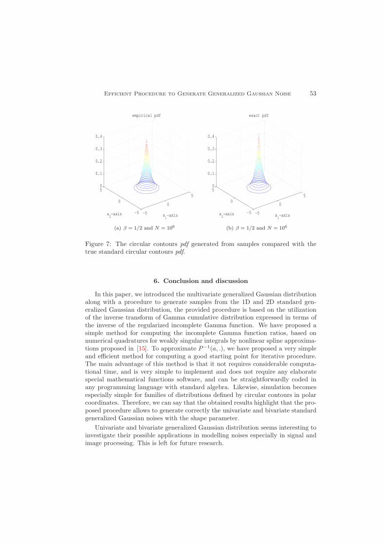
Figure 7: The circular contours pdf generated from samples compared with thetrue standard circular contours pdf.

6. Conclusion and discussion

In this paper, we introduced the multivariate generalized Gaussian distributionalong with a procedure to generate samples from the 1D and 2D standard gen-eralized Gaussian distribution, the provided procedure is based on the utilizationof the inverse transform of Gamma cumulative distribution expressed in terms ofthe inverse of the regularized incomplete Gamma function. We have proposed asimple method for computing the incomplete Gamma function ratios, based onnumerical quadratures for weakly singular integrals by nonlinear spline approxima-tions proposed in [15]. To approximate P−1(a, .), we have proposed a very simpleand efficient method for computing a good starting point for iterative procedure.The main advantage of this method is that it not requires considerable computa-tional time, and is very simple to implement and does not require any elaboratespecial mathematical functions software, and can be straightforwardly coded inany programming language with standard algebra. Likewise, simulation becomesespecially simple for families of distributions defined by circular contours in polarcoordinates. Therefore, we can say that the obtained results highlight that the pro-posed procedure allows to generate correctly the univariate and bivariate standardgeneralized Gaussian noises with the shape parameter.

Univariate and bivariate generalized Gaussian distribution seems interesting toinvestigate their possible applications in modelling noises especially in signal andimage processing. This is left for future research.


References

1. B. C. Arnold, E. Castillo, J. M. Sarabia, Multivariate distributions defined in terms of con-tours, Journal of Statistical Planning and Inference 138 (12), 4158-4171, 2008.

2. D.H. Bailey, J.M. Borwein, Crandall’s computation of the incomplete Gamma function andthe Hurwitz zeta function, with applications to Dirichlet L-series, Applied Mathematics andComputation, Vol 268, 462-477, 2015.

3. F. Chapeau-Blondeau, A. Monir, Numerical Evaluation of the Lambert W Function and Ap-plication to Generation of Generalized Gaussian noise with exponent 1/2, IEEE Transactionson Signal Processing, vol. 50, 2160-2165, 2002.

4. D. Cho, T. D. Bui, Multivariate statistical modeling for image denoising using wavelet trans-forms, Signal Processing: Image Communication, 20 (1), 77-89, 2005.

5. R.A. DeVore, G.G. Lorentz, Constructive approximation. Springer-Verlag, Berlin, 1993.

6. L. Devroye, Random variate generation for multivariate unimodal densities, ACM Transac-tions on Modeling and Computer Simulation, 7, 447-477, 1997.

7. A.R. DiDonato, A. H. Morris, Computation of the incomplete gamma function ratios andtheir inverse, ACM Trans. Math. Software, vol. 12 (4), 377-393, 1986.

8. M. Dohler, M. Arndt, Inverse incomplete gamma function and its application, ElectronicsLetters, vol. 42 No.1, pp. 6-35, 2006.

9. K. T. Fang, S. Kotz, and K. W. Ng , Symmetric Multivariate and Related Distributions,London: Chapman & Hall, 1987.

10. K. T. Fang, S. Kotz, and K. W. Ng , Symmetric Multivariate and Related Distributions,Monographs on Statistics and Applied Probability, 36, Chapman & Hall, New York, 1990.

11. A. Gil, J. Segura, and N. M. Temme, Numerical methods for special functions. SIAM,Philadelphia, PA, 2007.

12. A. Gil, J. Segura, N. M. Temme, Efficient and Accurate Algorithms for the Computation andInversion of the Incomplete Gamma Function Ratios, SIAM J. Scientific Computing, vol. 34(6), A2965-A2981, 2012.

13. E. Gomez, M.A. Gomez-Villegas and J.M. Marın Gomez, A multivariate gener- alization ofthe power exponential family of distributions, Commun. Statist.-Theory and methods, 27

(3), 589-600, 1998.

14. M. E. Johnson, Multivariate Statistical Simulation. Wiles Series in Probability and Mathe-matical Statistics, New York, 1987.

15. H. Kaneko, Y. Xu, Gauss-Type Quadratures for Weakly Singular Integrals and their Applica-tion to Fredholm Integral Equations of the Second Kind, Mathematics of Computation, vol.62, no. 206, 739-753, 1994.

16. D. Kelker, Distribution Theory of Spherical Distributions and Location-Scale Parameter Gen-eralization, Sankhya: The Indian Journal of Statistics, 32 (4), 419-430, 1970.

17. T. Luu, Efficient and accurate parallel inversion of the Gamma distribution, SIAM J. Sci.Comput., 37 (1), C122-C141, 2015.

18. A. Monir, Contribution a la modelisation et a la synthese des signaux aleatoires: signaux nongaussiens, signaux a correlation non exponentielle, these de doctorat, Universite d’AngersFrance, Novembre 2003.

19. A. Monir, H. Mraoui, Spline approximations of the Lambert W function and application tosimulate generalized Gaussian noise with exponent α = 1/2, Digital Signal Processing, vol.33, 34-41, 2014.

20. R. B. Paris, Incomplete gamma and related functions, NIST handbook of mathematicalfunctions, U.S. Dept. Commerce, Washington, DC, 175-192, 2010.


21. F. Pascal, L. Bombrun, J.-Y. Tourneret, and Y. Berthoumieu, Parameter estimation formultivariate generalized gaussian distributions, IEEE Transactions on Signal Processing, 61(23), 5960-5971, 2013.

22. W.H. Press, S.A. Teukolsky, W.T. Vetterling, B.P. Flannery, Numerical Recipes: The Art ofScientific Computing, third ed., Cambridge Univ. Press, Cambridge, 2007.

23. N. Solaro, Random variate generation from Multivariate Exponential Power distribution,Statistica &Applicazioni, vol. II, no. 2, 2004.

24. E. A. Valdez, A. Chernih, Wang’s capital allocation formula for elliptically contoured distri-butions, Insurance: Mathematics and Economics, 33, 517-532, 2003.

A Course of Modern Analysis, Cambridge University Press, Cambridge (1902); Fourth Edition(1965).

25. E.T. Whittaker, G.N. Watson, A Course Modern Analysis, Cambridge University Press,Cambridge (1902), Fourth Edition 1965.

Abdelilah Monir,Department of Mathematics (LMA),Faculty of Sciences,Moulay Ismail University of Meknes,Meknes, Morocco.E-mail address: [email protected]

and

Hamid Mraoui,Department of Computer Science,Faculty of Sciences (LaRI),Mohammed First University,Oujda, Morocco.E-mail address: hamid [email protected]

and

Abdeljabbar El Hilali,Department of Mathematics (LMA),Faculty of Sciences,Moulay Ismail University of Meknes,Meknes, Morocco.E-mail address: [email protected]

abstract - Universidade Estadual de Maringá

Documents

Transcript of abstract - Universidade Estadual de Maringá