digitalassets.lib.berkeley.edudigitalassets.lib.berkeley.edu/etd/ucb/text/Galanis... · ·...

Probabilistic Methods to Identify Seismically Hazardous

Older-Type Concrete Frame Buildings

By

Panagiotis Galanis

A dissertation submitted in partial satisfaction of the

requirements for the degree of

Doctor of Philosophy

in

Engineering – Civil and Environmental Engineering

in the

Graduate Division

of the University of California, Berkeley

Committee in charge

Professor Jack P. Moehle, Chair

Professor Khalid M. Mosalam

Professor David R. Brillinger

Fall 2014

1

ABSTRACT

Probabilistic Methods to Identify Seismically Hazardous Older-Type Concrete

Frame Buildings

By

Panagiotis Galanis

Doctor of Philosophy in Engineering – Civil and Environmental Engineering

University of California, Berkeley

Professor Jack P. Moehle, Chair

Earthquakes that have occurred recently across the globe in various countries including United

States, Japan, New Zealand, Haiti, Turkey and Italy have brought into light the poor seismic

performance of older-type, non-ductile concrete buildings. These buildings, mainly designed and

constructed prior to 1980s, lack proper seismic detailing and may pose an unacceptably high

seismic risk.

Non-ductile concrete buildings pose one of the greatest seismic safety problems in the world due

to the large amount of old buildings constructed in earthquake prone regions. It is indicative that

according to the Concrete Coalition and the California inventory project there are 16,000-17,000

of these buildings in high earthquake risk counties of California. Many of these buildings have

high occupancies, including residential, commercial and critical services. In case of a severe

earthquake, the severe damage or even collapse that could occur in these buildings could result in

large number of casualties.

While engineers generally recognize that proactive steps are required to address the risk posed by

these buildings, mitigation efforts are largely stymied by insufficient knowledge about the scale

of the problem, insufficient tools to identify the truly dangerous buildings, high costs of

strengthening, and owner resistance to pay for the strengthening with uncertain benefits. This

study constitutes an effort to identify seismically hazardous concrete frame buildings through

simplified methods that do not require complicated analysis.

Three idealized concrete frame buildings with different heights are used as archetypes. The study

attempts to link the collapse performance of these buildings with various structural deficiencies

that appear commonly in older construction practice. To evaluate the performance of these

buildings non-linear dynamic analysis for several far-fault ground motions is performed. The

analysis considers nonlinearities associated with flexural yielding, shear and axial failure. The

main deficiencies explored are development of weak story mechanisms due to strong column-

2

weak beam designs, brittle shear or axial failure modes associated with inadequate column shear

reinforcement detailing, and splicing and connectivity weaknesses between structural members.

The results indicate that the suggested methods can be used to assess the collapse risk of older-

type concrete buildings. The methods developed in the current study use simple engineering

parameters such as column-to-beam strength ratio and column flexural to shear strength ratio to

estimate the collapse risk of older type concrete buildings. A probabilistic approach is suggested

that takes into account record-to-record variability and could accommodate as well uncertainty

associated with structural properties and collapse modeling.

In Chapter 7 the proposed methodology is evaluated by applying it to the three idealized

buildings developed. The estimated probabilities of collapse calculated for each of the buildings

according to the proposed methodology are compared with the values provided by sophisticated

non-linear dynamic analyses. The results suggest that the proposed methodology successfully

identifies deficiencies that are leading to high collapse potential and provides an effective tool in

classifying collapse prone concrete frame buildings.

i

In memory of my grandfather, Andreas Mykoniatis

ii

ACKNOWLEDGMENTS

This work was supported mainly by the Fulbright Foundation through the International Fulbright

Science and Technology Award that the author received in 2009 to pursue doctoral studies in the

United States. Additional funding was provided by the U.S. National Science Foundation under

Award 0618804 and the Applied Technology Council, through the ATC-78 project.

While the writing of a dissertation may be a solitary experience, many people deserve my thanks

for the contributions they have provided along the way.

First of all, I would like to express my sincerest gratitude to my advisor Professor Jack Moehle.

His patient guidance, keen insights and persistence in finding practical solutions to challenging

problems have shaped not only this doctoral dissertation but also my entire approach to research.

I would like to thank particularly Professors Filip Filippou, Khalid Mosalam, Stephen Mahin and

David Brillinger for serving as members in my qualifying exam and dissertation committees and

for providing me with stimulating comments related to my research work.

I would also like to thank the committee members of the ATC-78 project including Ken Elwood,

Robert Hanson, Cody Harrington, John Heintz, William T. Holmes, Abbie Liel, Mike Mehrain,

Chris Rojahn, Siamak Sattar, and Peter Somers for their invaluable contributions and inputs. The

contribution of Francesca Renouard in the development of Appendix F is also acknowledged.

My friends and colleagues in the Department of Civil and Environmental Engineering at U.C.

Berkeley, namely, Grigoris Antonellis, Marco Broccardo, Veronique Le Corveque, Mayssa

Dabaghi, Pardeep Kumar, Simon Kwong, Mohamed Moustafa, Eleni Stavropoulou, Ahmet Can

Tanyeri, and Tea Visnijc, provided support and assistance for which I am grateful.

I am also grateful to Professor George Gazetas, Professor Elisavet Vintzileou, and Mr. Alkimos

Papathanasiou for being great mentors and for encouraging me to pursue doctoral studies.

I would like to express my deepest gratitude to my friends in Greece Giorgos Alexandrou,

Vassilis Dimoudis, Giorgos Karounos, Maria Tzoumanika, and Pantelis Vrachnelis for their

continuous support all these years.

Finally I am eternally grateful to my parents Iraklis and Ino. Their sacrifices and encouragements

made this degree and all my achievements in life a reality for me.

iii

TABLE OF CONTENTS

1 INTRODUCTION..............................................................................................................1

1.1 Motivation ................................................................................................................1

1.2 Brief History of Seismic Codes in California ..........................................................2

1.2.1 Non-Ductile Concrete Buildings..................................................................3

1.2.2 Buildings Designed after 1980s ...................................................................3

1.3 Scope of the Study ...................................................................................................3

1.4 Manuscript Organization .........................................................................................4

2 SEISMIC RISK EVALUATION OF OLDER-TYPE CONCRETE

BUILDINGS: THEORETICAL ASPECTS ....................................................................5

2.1 Collapse Simulation of Concrete Buildings .............................................................5

2.1.1 Column Models for Collapse Simulation ....................................................6

2.1.2 Haselton et al. (2008) ...................................................................................7

2.1.3 Elwood and Moehle (2002) .........................................................................9

2.1.4 Modeling Inadequate Lap-Splicing Conditions for the Column

Longitudinal Steel Reinforcement .............................................................12

2.1.5 Beam Column Joints for Collapse Simulation ...........................................14

2.2 Seismic Risk Assessment .......................................................................................18

2.2.1 Regress Using Unscaled Ground Motions (Cloud Analysis) ....................19

2.2.2 Scaling Records to the Target IM Level - IDA..........................................20

2.3 Identifying Parameters Influencing the Collapse Performance .............................26

2.4 Estimating Story Drift Demand .............................................................................28

2.5 Estimating Column Drift Capacity ........................................................................31

3 EVALUATION OF COLLAPSE SIMULATION OF CONCRETE FRAME

STRUCTURES .................................................................................................................36

3.1 Experimental Investigation ....................................................................................36

3.2 Input Ground Motions............................................................................................39

3.3 Material Properties .................................................................................................41

3.4 Comparison of Analytical Models with Test Results ............................................42

3.5 Summary of the Experimental Evaluation .............................................................61

iv

4 DEVELOPMENT OF ARCHETYPE BUILDINGS – COLLAPSE

SIMULATION MODELS ...............................................................................................62

4.1 Development of the Archetype Buildings..............................................................62

4.2 Analytical Modeling - Collapse Simulation Models .............................................66

4.2.1 Linear Elastic Stiffness Properties .............................................................66

4.2.2 Nonlinear Modeling for Flexure-Controlled Members..............................67

4.2.3 Nonlinear Modeling for Shear-Controlled Members .................................68

4.2.4 Dynamic Simulation ..................................................................................68

5 A STRENGTH-BASED APPROACH TO EVALUATE THE COLLAPSE

POTENTIAL OF OLDER-TYPE CONCRETE FRAME BUILDINGS ...................71

5.1 Pushover Analysis to Evaluate the Seismic Performance of Existing

Concrete Buildings.................................................................................................71

5.2 Assessment of Seismic Behavior ...........................................................................75

5.3 Using Collapse Indicators to Perform Earthquake Risk Assessement for

Existing Buildings ..................................................................................................78

5.4 Earthquake Risk Assessement for Buildings with Non-Uniform Structural

Parameters ..............................................................................................................87

5.5 Limitations of the Strength-Based Approach in Collapse Evaluation ...................90

6 A DISPLACEMENT-BASED METHODOLOGY TO EVALUATE THE

COLLAPSE POTENTIAL OF OLDER-TYPE CONCRETE FRAME

BUILDINGS .....................................................................................................................91

6.1 Determination of Story Drift Ratio Demand .........................................................91

6.1.1 Estimating Maximum Displacement at the Effective Height of the

Building......................................................................................................92

6.1.2 Estimating Maximum Story Drift ..............................................................96

6.2 Determination of Column Drift Capacity ............................................................110

6.3 A Methodology to Estimate the Column Failure Potential ..................................111

6.3.1 Estimating Column Drift Demand using only Hand Calculations...........111

6.3.2 Estimating Column Drift Capacity ..........................................................113

6.3.3 Estimating Column Failure Potential .......................................................115

6.4 Evaluation of the Story Collapse Potential ..........................................................116

6.5 Evaluation of the Building Collapse Potential .....................................................117

v

7 EVALUATION OF THE DISPLACEMENT-BASED METHOD FOR THE

IDEALIZED BUILDINGS ............................................................................................118

7.1 Evaluation of the Collapse Potential for the Idealized buildings .........................118

7.1.1 Evaluation of Collapse Potential for the 4-Story Idealized Building ......120

7.1.2 Evaluation of Collapse Potential for the 8-Story Idealized Building ......122

7.1.3 Evaluation of Collapse Potential for the 12-Story Idealized

Building....................................................................................................126

8 SUMMARY AND CONCLUSIONS ............................................................................129

8.1 Collapse Simulation .............................................................................................130

8.2 Collapse Indicators – a Strength-Based Approach for Collapse Evaluation .......131

8.3 A Displacement-Based Approach for Collapse Evaluation .................................132

8.4 Recommendations for Future Study ....................................................................133

REFERENCES ...........................................................................................................................135

A. DESIGN PARAMETERS OF THE IDEALIZED BUILDINGS ..............................141

B. RECALIBRATION OF HASELTON ET AL. FLEXURE- CONTROLLED

MODEL PARAMETERS .............................................................................................163

C. EIGENVALUE ANALYSIS OF THE STUDIED BUILDINGS ...............................165

D. AN APPROXIMATE PROCEDURE TO ESTIMATE THE BASE SHEAR

CAPACITY OF CONCRETE FRAME BUILDINGS ...............................................168

E. COLLAPSE PERFORMANCE TABLES FOR THE IDEALIZED

BUILDINGS ...................................................................................................................173

F. APPROXIMATE RELATIONSHIPS TO ESTIMATE THE

FUNDAMENTAL BUILDING PERIOD ....................................................................184

G. STORY DRIFT PROFILES .........................................................................................198

vi

LIST OF FIGURES

Figure 2.1 Simulated collapse modes for concrete frames: ...................................................... 6 Figure 2.2 Backbone curve of the component model suggested by Ibarra .............................. 7 Figure 2.3 Illustration of the components utilized by the model suggested by Haselton et al. 8 Figure 2.4 Illustration of the components utilized in the limit-state model using a lumped

plasticity approach ................................................................................................ 10

Figure 2.5 Shear and axial response according to the limit state material ............................. 11 Figure 2.6 Normalized moment – lateral drift ratio for columns with inadequate lap splicing

conditions for far fault displacement histories ...................................................... 13 Figure 2.7 Assumed zero-length plastic hinge rotational behavior for inadequate lap-splicing

conditions .............................................................................................................. 14

Figure 2.8 Proposed scissors model (Hassan and Moehle, 2012) .......................................... 15 Figure 2.9 Proposed backbone curve of joint shear stress strain (Hassan and Moehle, 2012) ..

............................................................................................................................... 16

Figure 2.10 Axial load-drift ratio relationship at axial failure for exterior and corner joints

(Hassan 2013) ....................................................................................................... 17

Figure 2.11 Estimating the conditional distribution of EDP | IM at Sa(T1) using “cloud

analysis” (a) conditional mean value from linear regression (b) comparison of

strip of EDP data Gaussian CCDF based on linear regression ............................. 19

Figure 2.12 Multiple stripes of data for different IM Levels (Baker 2007) .......................... 21 Figure 2.13 Development of fragility curves ........................................................................... 26

Figure 2.14 Approach for establishing collapse indicator limits. Example collapse fragilities

for different collapse indicator values ................................................................... 28

Figure 2.15 5-story SMRF (Shome, 1999) ............................................................................... 29 Figure 2.16 20-story SMRF (Gupta, 1999) .............................................................................. 29 Figure 2.17 Backbone curve of component force-deformation response in ASCE-41 ............ 32

Figure 2.18 Comparison of column deformation capacity values provided by different models

............................................................................................................................... 34

Figure 3.1 Reinforced concrete column specimen details: ..................................................... 38 Figure 3.2 Experimental setup................................................................................................ 38 Figure 3.3 Filtered Llolleo input ground motion (Chile 1985) ; ............................................ 40

Figure 3.4 Filtered Kobe Input Ground Motion (Japan 1995): .............................................. 40 Figure 3.5 Comparison of Test 1 results with the Haselton model ........................................ 46 Figure 3.6 Comparison of Test 2 results with the Haselton model ........................................ 46 Figure 3.7 Comparison of Test 3 results with the Haselton model ........................................ 47 Figure 3.8 Comparison of Test 4 results with the Haselton model ........................................ 47

Figure 3.9 Comparison of Test 5 results with the Haselton model ........................................ 48 Figure 3.10 Comparison of Test 6 results with the Haselton model ........................................ 48 Figure 3.11 Comparison of Test 7 results with the Haselton model ........................................ 49 Figure 3.12 Comparison of Test 8 results with the Haselton model ........................................ 49

Figure 3.13 Comparison of Test 9 results with the Haselton model ........................................ 50 Figure 3.14 Comparison of Test 10 results with the Haselton model ...................................... 50 Figure 3.15 Comparison of Test 11 results with the Haselton model ...................................... 51 Figure 3.16 Comparison of Test 4 Results with the Elwood model ......................................... 51

vii

Figure 3.17 Comparison of Test 6 results with the Elwood model .......................................... 52

Figure 3.18 Comparison of Test 10 results with the Elwood model ........................................ 52 Figure 3.19 Comparison of Test 3 results with the Haselton model with λ=λmean+λstd ........... 53 Figure 3.20 Comparison of Test 9 results with the Haselton model with λ=λmean+λstd ............ 54

Figure 3.21 Comparison of Test 1 results with the Haselton - Elwood model ........................ 55 Figure 3.22 Comparison of Test 2 results with the Haselton - Elwood model ........................ 55 Figure 3.23 Comparison of Test 7 results with the Haselton - Elwood model ........................ 56 Figure 3.24 Comparison of Test 8 results with the Haselton - Elwood model ........................ 56 Figure 4.1 Three- dimensional view of the studied buildings ................................................ 63

Figure 4.2 Schematic elevation view of the simulated frames ............................................... 64 Figure 4.3 Lumped plasticity model....................................................................................... 67 Figure 4.4 Empirical and fitted log-normal cumulative distribution function of probability of

collapse ................................................................................................................. 69

Figure 5.1 Pushover analysis of the three “modern code design” building models ............... 72 Figure 5.2 Failure mechanisms of the three “modern code design” building models ............ 73

Figure 5.3 Pushover analysis of the 8-Story building models for different ΣΜnc/ΣΜnb ratios ..

............................................................................................................................... 74

Figure 5.4 Failure mechanisms of the 8-Story building models for different ΣΜnc/ΣΜnb

ratios ...................................................................................................................... 75 Figure 5.5 Incremental Dynamic Analysis (IDA) curves for the 8-story “modern code

design” building model ......................................................................................... 76 Figure 5.6 Collapse fragility functions of the “modern code design” building models ......... 77

Figure 5.7 Comparison of collapse performance of the studied building models for Re=3 and

Vp/Vn=0.6 ............................................................................................................ 79 Figure 5.8 Collapse Performance of (a) 4-Story (b) 8-Story (c) 12-Story building models

with Vp/Vn=0.6 ..................................................................................................... 80

Figure 5.9 Comparison of the fragility curves of the 8-Story Building having ΣΜnc/ΣΜnb=1.2

............................................................................................................................... 81 Figure 5.10 Comparison of the collapse performance of the three Idealized Buildings for

ΣΜnc/ΣΜnb=1.2 and Re=3 ...................................................................................... 82 Figure 5.11 Comparison of the collapse performance of the 4-Story Building for

(a) Vp/Vn=0.6 , (b) Vp/Vn=0.8, (c) Vp/Vn=1.0 and (d) Vp/Vn=1.2 ........................... 83 Figure 5.12 Comparison of the collapse performance of the 8-Story Building for

(a) Vp/Vn=0.6 , (b) Vp/Vn=0.8, (c) Vp/Vn=1.0 and (d) Vp/Vn=1.2 ........................... 84 Figure 5.13 Comparison of the collapse performance of the 12-Story Building for

(a) Vp/Vn=0.6 , (b) Vp/Vn=0.8, (c) Vp/Vn=1.0 and (d) Vp/Vn=1.2 ........................... 85 Figure 5.14 Comparison of the collapse performance of the three Idealized Buildings with

Re=3 for (a) Vp/Vn=0.6 , (b) Vp/Vn=0.8 , (c) Vp/Vn=1.0 and (d) Vp/Vn=1.2 ....... 86

Figure 5.15 Illustration of joins A,B,C,D,E, and F of the 8-story idealized building .............. 87 Figure 5.16 Comparison of the collapse performance of the idealized 8-story building with:

a) uniform ΣΜnc/ΣΜnb values, and b) non-uniform ΣΜnc/ΣΜnb values ................ 89 Figure 6.1 Ratio of (maximum displacement at effective modal height of non-linear analysis

(IDA)) / (estimated displacement at effective modal height of equation 6.1) for

different R indices of the 8-Story building (Vp/Vn=0.6) ........................................ 96 Figure 6.2 Two idealized story drift patterns for an example building frame ........................ 97

viii

Figure 6.3-a Alpha coefficient story profiles for different variations of the 4-story idealized

buildings ................................................................................................................ 99 Figure 6.3-b Alpha coefficient value at the 1

st story for different variations of the 4-story

idealized building ................................................................................................ 100


buildings .............................................................................................................. 101 Figure 6.4-b Alpha factor coefficient at the 1

st story for different variations of the 8-story

idealized building ................................................................................................ 102 Figure 6.5-a Alpha coefficient story profiles for different variations of the 12-story idealized

buildings .............................................................................................................. 103 Figure 6.5-b Alpha factor coefficient at the 1st story for different variations of the 12-story

idealized building ................................................................................................ 104 Figure 6.6-a Comparison of the alpha coefficient story profiles for the 8-story with uniform

DCRs (idealized building) and with critical story at the mid-height (Vp/Vn=0.8 for

both cases) (for the critical 4th

story case DCR4th=1.30DCR1st) ......................... 105

Figure 6.6-b Comparison of the alpha coefficient values at the critical story for the 8-story with

uniform DCRs (idealized building) and with critical story at the mid-height

(Vp/Vn=0.8 for both cases) (for the critical 4th

story case DCR4th=1.30DCR1st) . 106 Figure 6.7 Assumed zero-length plastic hinge rotational behavior for inadequate lap-splicing

conditions ............................................................................................................ 107

Figure 6.8-a Comparison of the alpha coefficient story profiles for different variation of the

8-story idealized building with adequate and inadequate lap splicing conditions at

the base of the 1st story (Vp/Vn=0.8 for both cases) ............................................. 108

Figure 6.8-b Comparison of the alpha coefficient value at the critical 1st story for different

variations of the 8-story idealized building with adequate and inadequate lap

splicing conditions at the base of the 1st story (Vp/Vn=0.8 for both cases) ......... 109

Figure 6.9 Illustration of the calculation of axial load for the critical 1st story of the 4-story

idealized building ................................................................................................ 114 Figure 7.1 Uniform Hazard Spectra (UHS) for the idealized buildings located at Berkeley,

CA (Site Class D)................................................................................................ 119 Figure A.1 Three- dimensional view of the studied buildings .............................................. 142

Figure A.2 Plan view of the archetype idealized buildings................................................... 143 Figure A.3 Schematic elevation view of the 4-story archetype building .............................. 145

Figure A.4 Schematic elevation view of the 8-story archetype building .............................. 147 Figure A.5 Schematic elevation view of the 12-story archetype building ............................ 149 Figure C.1 Eigenvectors of 1

st and 2

nd modes, 4-story building ........................................... 165

Figure C.2 Eigenvectors of 1st and 2

nd modes, 8-story building ........................................... 166


nd modes, 12-story building ......................................... 167

Figure D.1 Schematic Drawing for the calculation of story plastic shear capacity .............. 169 Figure F.1 Schematic illustration of the generic frame model used to represent the idealized

8-story building ................................................................................................... 186 Figure F.2 Effect of building height (H) on the fundamental period T1 of the building ....... 190 Figure F.3 Effect of normalized base shear strength (V/W) on the fundamental period T1 of

the building ......................................................................................................... 190 Figure F.4 Effect of longitudinal reinforcement ratio (ρlong) on the fundamental period T1 of

the building ......................................................................................................... 191

ix

Figure F.5 Comparison of relationships for estimation of the fundamental building period 193

Figure F.6 Comparison of relationships for estimation of the fundamental building period

with analytical data (Effect of V/W on T1) ......................................................... 195 Figure F.7 Comparison of relationships for estimation of the fundamental building period

with analytical data (Effect of H on T1) .............................................................. 196 Figure G.1 Observed story drift ratio demand (δ1/h1) at the 1

st story over estimated average

drift (δeff/heff) ....................................................................................................... 200

x

LIST OF TABLES

Table 2.1 Far-field record set used in the current study........................................................ 23 Table 2.2 Far-field ground motion parameter information ................................................... 24 Table 2.3 Critical seismic deficiencies found in pre-1980 concrete buildings ..................... 27 Table 2.4 Regression relationships of maximum story drift and different intensity measures

............................................................................................................................... 30 Table 2.5 Classification of column condition ...................................................................... 32 Table 2.6 Column deformation capacities according to column condition ......................... 33 Table 2.7 Column deformation capacities for condition iii columns .................................... 34 Table 3.1 Test matrix ............................................................................................................ 39

Table 3.2 Concrete mean strength properties........................................................................ 41

Table 3.3 Steel reinforcement mean strength properties ....................................................... 41

Table 3.4 Column modeling properties................................................................................. 43 Table 3.5 Modeling parameters (Haselton model)................................................................ 43

Table 3.6 Modeling parameters (Elwood model) ................................................................. 44 Table 3.7 Fundamental Period and damping ratio ................................................................ 45

Table 3.8 Actual test results .................................................................................................. 57 Table 3.9 Haselton analytical model results ......................................................................... 58 Table 3.10 Elwood analytical model results ........................................................................... 59

Table 3.11 Haselton-Elwood analytical model results............................................................ 60

Table 3.12 Haselton analytical model results with λ= λmean+λstd ............................................ 61

Table 4.1 Combinations of Vp/Vn and ΣMnc/ΣMnb considered in the current study ............... 65 Table 4.2 Modification factor values for the cracked stiffness properties of the structural

members ................................................................................................................ 66

Table 5.1 Combination of non-uniform join ΣΜnc/ΣΜnb values ........................................... 88

Table 6.1 Coefficients of the studied buildings utilized in equation 6.1 .............................. 93 Table 6.2 Mean ratio of (maximum displacement at effective modal height floor level of

non-linear analysis) / (estimated displacement at effective modal height floor level

of equation 6.1) for different Vp/Vn and ΣMnc/ΣMnb ratios of the 4-Story Idealized

Building................................................................................................................. 94

Table 6.3 Mean ratio of (maximum displacement at effective modal height floor level of


of equation 6.1) for different Vp/Vn and ΣMnc/ΣMnb ratios of the 8-Story Idealized

Building................................................................................................................. 94 Table 6.4 Mean ratio of (maximum displacement at effective modal height floor level of


of equation 6.1) for different Vp/Vn and ΣMnc/ΣMnb ratios of the 12-Story

Idealized Building ................................................................................................. 95 Table 6.5 Values of αx for buildings with 1

st Story Critical................................................ 112

Table 6.6 Uncertainty in predictions of drift demand ......................................................... 113 Table 7.1 Spectral acceleration values used for the collapse evaluation ............................ 120 Table 7.2 Comparison of collapse evaluation using the displacement-based methodology

and IDA for the 4-story idealized building ......................................................... 121

xi

Table 7.3 Comparison of collapse evaluation using the displacement-based methodology

and IDA for the 8-story idealized building ......................................................... 123 Table 7.4 Comparison of collapse evaluation using the displacement-based methodology

and IDA for the 8-story idealized building with inadequate lap splicing conditions

at the base of the 1st story ............................................................................. 125

Table 7.5 Comparison of collapse evaluation using the displacement-based methodology

and IDA for the 8-story idealized building with weak story at the mid-height .. 126 Table 7.6 Comparison of collapse evaluation using the displacement-based methodology

and IDA for the 12-story idealized building ....................................................... 127

Table A.1 Interior column reinforcement schedule of the 4-story archetype building ........ 145 Table A.2 Corner column reinforcement schedule of the 4-story archetype building ......... 146 Table A.3 Beam reinforcement schedule of the 4-story archetype building ....................... 146 Table A.4 Interior column reinforcement schedule of the 8-story archetype building ........ 147

Table A.5 Corner column reinforcement schedule of the 8-story archetype building ......... 148 Table A.6 Beam reinforcement schedule of the 8-story archetype building ....................... 148

Table A.7 Interior column reinforcement schedule of the 12-story archetype building ...... 150 Table A.8 Corner column reinforcement schedule of the 12-story archetype building....... 151

Table A.9 Beam reinforcement schedule of the 12-story archetype building ..................... 152 Table A.10 Reinforcement and modeling parameter details of the 4-story building for the case

of Vp/Vn=0.6 (Archetype 4-story building) ......................................................... 153

Table A.11 Reinforcement and modeling parameter details of the 4-story building for the case

of Vp/Vn=0.8 ........................................................................................................ 153


of Vp/Vn=1.0 ........................................................................................................ 154 Table A.13 Reinforcement and modeling parameter details of the 4-story building for the case

of Vp/Vn=1.2 ........................................................................................................ 154


of Vp/Vn=0.6 (Archetype 8-story building) ......................................................... 155 Table A.15 Reinforcement and modeling parameter details of the 8-story building for the case

of Vp/Vn=0.8 ...................................................................................................... 156 Table A.16 Reinforcement and modeling parameter details of the 8-story building for the case

of Vp/Vn=1.0 ........................................................................................................ 157 Table A.17 Reinforcement and modeling parameter details of the 8-story building for the case

of Vp/Vn=1.2 ........................................................................................................ 158 Table A.18 Reinforcement and modeling parameter details of the 12-story building for the

case of Vp/Vn=0.6 (Archetype 12-story building) ............................................... 159 Table A.19 Reinforcement and modeling parameter details of the 12-story building for the

case of Vp/Vn=0.8 ................................................................................................ 160

Table A.20 Reinforcement and modeling parameter details of the 12-story building for the

case of Vp/Vn=1.0 ................................................................................................ 161

Table A.21 Reinforcement and modeling parameter details of the 12-story building for the

case of Vp/Vn=1.2 ................................................................................................ 162 Table D.1 Comparison of pushover and estimated maximum base shear capacity of the

4-story building ................................................................................................... 171 Table D.2 Comparison of pushover and estimated maximum base shear capacity of the

8-story Building .................................................................................................. 171

xii

Table D.3 Comparison of pushover and estimated maximum base shear capacity of the

12-story building ................................................................................................. 172 Table E.1 Probability of collapse matrix for the 4-story building with Vp/Vn = 0.6

(Re normalization factor) ..................................................................................... 173

Table E.2 Probability of collapse matrix for the 4-story building with Vp/Vn = 0.8

(Re normalization factor) ..................................................................................... 174 Table E.3 Probability of collapse matrix for the 4-story building with Vp/Vn = 1.0













Table E.13 Probability of collapse matrix for the 4-story building with Vp/Vn=0.6

(M normalization factor) ..................................................................................... 179 Table E.14 Probability of collapse matrix for the 4-story building with Vp/Vn=0.8





(M normalization factor) ..................................................................................... 181







xiii




Table F.1 Comparison of eigenvalue analysis of the idealized building models and the

equivalent generic frame model .......................................................................... 189 Table F.2 Regression parameters for model TG.F.,1 ............................................................. 192 Table F.3 Regression parameters for model TG.F.,2 ............................................................. 192 Table F.4 Comparison of eigenvalue analysis of the idealized building models and the

estimated building period values ........................................................................ 196

Table G.1.a Least squares estimation results of αx =exp (0β ) for the idealized 4- story building

............................................................................................................................. 201

Table G.1.b Least squares estimation results of

x

x

h

δln,

σ for the idealized 4- story building ..... 202


............................................................................................................................. 203


x

x

h

δln,

σ for the idealized 8- story building ...... 204

Table G.3.a Least squares estimation results of αx =exp (0β ) for the idealized 12- story

building ............................................................................................................... 205


x

x

h

δln,

σ for the idealized 12- story building .... 207

Table G.4.a Least squares estimation results of αx =exp ( 0β ) for the idealized 8- story building

with critical story at the mid-height ( DCR4th=1.30DCR1st ) .............................. 209


x

x

h

δln,

σ for the idealized 8- story building with

critical story at the mid-height ( DCR4th=1.30DCR1st )....................................... 210

Table G.5.a Least squares estimation results of αx =exp ( 0β ) for the idealized 8- story building

with inadequate lap splicing conditions at the base of the 1st story .................... 211


x

x

h

δln,

σ for the idealized 8- story building

inadequate lap splicing conditions at the base of the 1st story ............................ 212

1

1 Introduction

1.1 MOTIVATION

Strong earthquakes are not very frequent phenomena. When they occur, however they can have

destructive consequences. In recent years, earthquakes in Haiti, Chile, New Zealand and Japan

demonstrated the potentially large impact in the economies of those countries. This has raised a

new challenge for the 21st century regarding the appropriate earthquake design of structures so

that the casualties occurring due to such phenomena can be limited. It has also raised the

challenge of identifying potentially hazardous existing buildings.

The United States and especially the earthquake prone state of California have suffered several

times in the past by strong earthquakes. The impact of a major earthquake striking the City of

Los Angeles nowadays would be substantial. Sophisticated models estimate that property

damages would be greater than $20 billion, in addition to a large number of fatalities. Thus,

many federal agencies and private institutions, recognizing the need and the challenge of

mitigating the high seismic risk posed by collapse of specific structures, have devoted a

significant portion of their research activity towards mitigation of that problem.

Concrete is a popular building material in regions with high seismicity. In most instances,

concrete performs well. However, in order to do so, it needs to be properly proportioned and

detailed. This was proved by various past earthquakes, including the 1971 San Fernando

earthquake, the 1989 Loma Prieta earthquake, and the 1994 Northridge earthquake, where many

concrete buildings were seriously damaged or even collapsed with fatal consequences for their

occupants. These events have triggered discussions among the engineering community

concerning the largest magnitude earthquake that could be generated by known faults as well as

how buildings should be detailed to minimize earthquake loss. Recognizing the potential losses,

U.S. seismic codes have been improved significantly starting in the mid-1970s, especially as

regards the proportioning and detailing of reinforced concrete construction.

The lack of proper seismic detailing of older buildings renders them seismically vulnerable in

case of a strong earthquake. Contrary to new construction that follows seismic proportioning and

detailing to enable ductile response, older buildings commonly have non-ductile seismic

performance with low strength and deformation capacity. These buildings constitute a significant

safety concern in United States and around the world and are commonly referred to as non-

ductile concrete buildings.

The seismic risk posed by older concrete buildings was demonstrated in the 1971 San Fernando

earthquake. In that event the Olive View Hospital, a recently constructed building, almost

2

collapsed and an older concrete Veteran Administration Hospital building collapsed and killed

over 40 occupants. Since that time, the overall life-safety risk from older concrete buildings often

has been compared to unreinforced masonry buildings (URM).

Although various programs to mitigate the risk of URM buildings are common in zones of high

seismicity in the United States, no such programs have been implemented for older concrete

buildings. Some reasons that explain the lack of seismic risk programs for concrete buildings

include:

It is often difficult to visually determine seismic deficiencies in concrete buildings.

Careful studying of drawings, on-site inspection of the considered building and

supplemental sophisticated linear or non-linear analysis might be required to identify

seismically hazardous buildings

While various studies have suggested that older concrete buildings are very hazardous,

exposing their occupants to unacceptably high life-safety risk, past experience following

major earthquakes indicates that these buildings, while vulnerable to structural damage,

do not have high collapse rates in most parts of the world.

Concrete buildings are often large, the occupancy is high and ownership groups are often

politically powerful and resistant to seismic retrofitting because of its high costs and

extensive service disruption.

Current evaluation and retrofit code standards (ASCE/SEI 31, “Seismic Evaluation of

Existing Buildings” and ASCE/SEI 41, “Seismic Rehabilitation of Existing Buildings”)

are considered by many engineers in practice to be overly conservative and expensive to

implement.

A premise of the present study is that, if a reliable and inexpensive evaluation technique was

available, both authorities and building owners/tenants would act proactively to quantify the

collapse risk of older buildings and take action to mitigate the risk accordingly.

1.2 BRIEF HISTORY OF SEISMIC CODES IN CALIFORNIA

Building codes have seen major developments over the past century. The highest risk from

existing concrete buildings occurs because a significant number of them constructed in the 20th

century in the United States were designed prior to important developments in the building code

seismic requirements.

The earliest seismic design provisions in the United States were introduced in the Appendix of

the 1927 Uniform Building Code (UBC) after the 1925 Santa Barbara earthquake. After the

damages observed in the 1933 Long Beach Earthquake, the state of California, introduced the

Field Act and Riley Act that endorsed early design requirements for public buildings.

In 1957 the Structural Engineers Association of California published the first edition of

“Recommended Lateral Force Requirements and Commentary.” However the seismic design

provisions remained in the Appendix of the UBC until the International Conference of Building

Officials adopted seismic design provisions into the main code in 1961.

3

1.2.1 Non-Ductile Concrete Buildings

“Design of Multistory Reinforced Concrete Buildings for Earthquake Motions (Blume et al.,

1961) introduced modern concepts for earthquake-resistant reinforced concrete buildings. The

recommendations of this book influenced many engineers, but its recommendations were not

required by the building codes until after the 1971 San Fernando earthquake. The 1976 Uniform

Building Code introduced the requirement for special detailing of concrete frames in addition to

incorporation of larger seismic design loads than were required in previous code provisions.

Most engineers consider 1976 a critical date before which concrete frames equivalent to the

present day ductile moment resisting frames were not fully implemented in the design of

buildings. Buildings designed prior to 1976 correspond to the older-type construction that this

study is mainly attempting to evaluate. Due to the lack of adequate detailing in most of the cases,

these buildings are susceptible to brittle failure modes and thus are termed as non-ductile

concrete buildings to distinguish them from buildings constructed after this date.

1.2.2 Buildings Designed after 1980s

A common practice for buildings has been to have portions of the structure that are designed to

carry seismic forces while having others designed to carry only gravity loads. Some frames

designed as gravity-only frames experienced extensive damages in the 1994 Northridge

earthquake leading to strict requirements for proportioning and detailing of those frames in ACI

318-95. Buildings designed in the State of California after 1995, if proportioned appropriately

according to the prevailing design provisions, are considered to have adequate collapse

resistance for earthquake loading equal to what is assumed in today’s design practice (probability

of collapse for the Maximum Considered Earthquake shaking intensity approximately equal to

10%).

1.3 SCOPE OF THE STUDY

The current study presents evaluation methodologies to determine the collapse risk of older

concrete buildings designed prior to 1980s. The intent is to enable identification of relatively few

buildings in this class that have high collapse propensity without the need for extensive testing or

sophisticated nonlinear dynamic analysis. It is expected that evaluation of entire inventories of

this structural class would thus be affordable and feasible and the concrete buildings posing the

greatest threat of life loss could be potentially mitigated.

The evaluation methods described in the current study are limited to reinforced concrete frame

type structures with rigid diaphragms. However the method could be expanded in the future to

cover other concrete building systems, particularly those with walls or masonry infill walls.

4

1.4 MANUSCRIPT ORGANIZATION

This dissertation is organized in eight chapters, with specific content identified below.

Chapter 2 provides literature review corresponding to collapse modeling, seismic risk evaluation

methodologies and other theoretical aspects corresponding to identifying seismically hazardous

older-type concrete buildings.

Chapter 3 presents an analytical and experimental study of eleven scaled concrete frames with

different reinforcement details. The chapter includes descriptions of the tests performed as well

as analytical modeling techniques. The results provide insight into the effectiveness of the

modeling tools used in subsequent chapters.

Chapter 4 provides information on the development of the archetype buildings that were utilized

for the calibration of the methodology. The chapter also describes state of the art simulation tools

that were used to model the non-linear dynamic response and assess the collapse performance of

the considered buildings.

Chapter 5 presents a strength-based approach that could be used to evaluate the seismic

performance of buildings. The method explores the use of collapse indicators, that is, easy-to-

calculate engineering parameters, to estimate the collapse risk.

Chapter 6 presents a displacement-based approach to evaluate the seismic performance of

buildings. Calibration of the methodology is presented and consequently tested for the

considered buildings.

Chapter 7 evaluates the displacement based approach presented in Chapter 6. The methodology

proposed in Chapter 6 is applied for the three idealized buildings developed in Chapter 4 and the

results are compared with those derived from sophisticated non-linear dynamic analyses for the

studied buildings.

Chapter 8 presents a summary of research findings and conclusions as well as a list of topics for

future research.

5

2 Seismic Risk Evaluation of Older-Type Concrete

Buildings: Theoretical Aspects

The current chapter provides background information regarding basic aspects of the

methodology. The Chapter begins with a review of the modeling techniques used in the current

study to simulate collapse. Considerations regarding the applicability and the assumptions

involved are also discussed. Consequently the definition of seismic risk analysis is provided

along with two methods to perform structural vulnerability analysis and derive fragility curves.

The chapter concludes with a discussion of how collapse can be identified by using simple

engineering parameters and how story drift demand and column drift capacity can be defined in a

probabilistic framework.

2.1 COLLAPSE SIMULATION OF CONCRETE BUILDINGS

The last years there has been a great interest related to building code performance objectives

(performance-based design). One very important issue that has arisen lately has been life-safety

performance, which is primarily governed by structural collapse. Advances in computational

power and state of the art simulation tools have enabled development of non-linear seismic

analysis numerical models that allow simulation of structural collapse.

Two main failure modes for building collapse are considered in the current study:

a) Side-sway collapse is caused due to excessive story drifts in one story. The combination of the

earthquake lateral forces and the P-Delta effects result in large story drifts that cause the

structure to collapse in a sideways manner.

b) Vertical collapse is one of the most common collapse modes for older-type concrete buildings.

It is mainly caused by column members that are lightly confined. Such members are susceptible

to shear failures, which after a certain story drift level lead to inability of the damaged members

to support the axial loads due to gravity.

Figure 2.1 provides an illustration of the collapse modes considered in the current study.

6

Figure 2.1 Simulated collapse modes for concrete frames:

(a) Side-sway collapse, (b) Vertical collapse

Although in the literature there are a variety of sophisticated simulation tools to evaluate the non-

linear flexural response of structural components and collapse due to the side-sway mechanism,

only recently there have been efforts to develop analytical models for shear-critical columns,

with the ultimate goal of understanding the vertical collapse risk of existing buildings.

2.1.1 Column Models for Collapse Simulation

Columns are one of the most important structural components in the building since they are

transferring both the lateral and gravity loads to the foundation soil. Thus, the dynamic

performance of column members is a main emphasis of many collapse studies.

Several models exist in the literature for simulating the inelastic dynamic response of column

members at collapse. Important model characteristics include the following (Ghannoum, 2013):

Computational Efficiency. Collapse simulation studies require a large number of

simulations up to structural collapse. Therefore, models with high computational

efficiency may be preferred to more accurate modeling techniques. The main models that

satisfy this requirement correspond to center-line elements with lumped-plasticity or

fiber-section implementations.

Calibration to a wide range of column failure modes. The considered models should

be calibrated using laboratory data that account for different failure models.

Ability to simulate shear and axial degrading behavior, including both in-cycle and

cyclic degradation. In-cycle degradation is directly related with the incorporation of the

post-peak negative stiffness branch in the backbone curve of models simulating flexural,

shear or axial degradation. It has been observed that members subjected to long duration

motions with large number of cycles experience strength degradation due to cyclic

loading.

Available models in the current literature that satisfy most of the characteristics listed above

include those of Elwood and Moehle (2002) , Haselton et al. (2008), and Leborgne and

7

Ghannoum (2012). The first two of these are used in the present study. These are described

below.

2.1.2 Haselton et al. (2008)

In 2005 Ibarra et al. developed a model that was capable of modeling strength deterioration that

precipitates side-sway collapse. The model was implemented in OpenSees based on the Clough

hysteretic model. This model consists of a tri-linear monotonic backbone curve and includes

aspects of hysteretic model response related to cyclic strength and stiffness deterioration.

The developed model requires the specification of seven parameters to control the monotonic

and cyclic response. The parameters are: My; Mc/My; Ke; θcap,pl; θpc; λ; and c, each shown

schematically in Figure 2.2.

Figure 2.2 Backbone curve of the component model suggested by Ibarra

In 2008 , Haselton et al. (PEER 2007/03), used a database of 255 rectangular columns provided

by Berry et al. (2004) to calibrate the parameters utilized by the element model developed by

Ibarra et al.

The proposed model by Haselton follows a lumped-plasticity approach with zero-length

rotational springs placed at the ends of the elastic line elements. The zero-length springs are

assumed to account for non-linear material response. Figure 2.3 shows the arrangement of the

components according to the lumped plasticity approach suggested by Haselton et al.

8

Figure 2.3 Illustration of the components utilized by the model suggested by Haselton et al.

The zero-length parameters were calibrated by Haselton et al. using regression estimates that

matched the responses observed in laboratory tests and the lumped plasticity model. The

calibrations were based on mean values and are supposed to be less conservative than the values

provided by ASCE-41.

The column database used for calibration consists of 220 column tests of column members that

failed in flexure and 35 (255 columns in total) that failed in a flexure-shear failure mode. The

model was not calibrated for columns that sustain shear failure prior to flexural yielding. The

interested reader can find the calibrated model parameters for each of the 255 laboratory tests as

well as the suggested parameter relationships in Haselton et al. (2008).

In the original formulation the regression estimates were not distinguished between flexure and

flexure-shear failure. Dr. Liel and her colleagues re-calibrated the regression relationships such

that only columns that were reported to fail in flexure were included (ATC-78,2013). The

updated relationships suggested by this re-calibration are provided in Appendix B.

Although the model has the advantage of defining through regression the parameters that should

define the column response, the model does not distinguish between flexure and flexure-shear

failure. Thus this model cannot explicitly model shear-induced axial failure. This limitation

renders the model more applicable for collapse simulations where the columns are flexure-

controlled and the collapse failure is governed by a side-sway mechanism.

For the reasons suggested above and after the evaluation of the model suggested by Haselton

using laboratory tests (Chapter 3) , in the current study it was decided to use this modeling

technique for collapse simulation only for columns that are flexure-critical. This will be

explained further in Chapter 4.

9

2.1.3 Elwood and Moehle (2002)

Elwood and Moehle (2002) used a set of 50 tests compiled by Sezen (2002) to develop an

empirical model that relates the shear demand to the drift at shear failure. The relationship

defines a failure surface based on the transverse reinforcement ratio and axial loading ratio of the

member. If the shear demand exceeds a specified limit, shear failure is triggered. Similar to the

limit surface defined for the shear failure an empirical relationship that relates the axial demand

with the drift at axial failure was suggested. Equations 2.1 and 2.2 provide the proposed

relationships that define the failure surfaces for the shear and axial failure correspondingly.

100

1

'*40

1

'500

1"4

100

3

cgc

s

fA

P

f

v

L (Eq. 2.1)

)tan

(tan

)(tan1

100

4 2

cyst

a

dfA

sP

L

(Eq. 2.2)

where ρ” corresponds to the transverse reinforcement ratio, s is the spacing of transverse

reinforcement (given in inches), fy is the reinforcing steel yield strength (given in psi) , dc is the

depth of the column core from center line to center line of the ties (given in inches) , Ast is the

transverse reinforcement area (given in inches2), ν is the shear stress demand (given in psi), f’c is

the concrete strength (given in psi), P is the axial force (given in pounds) , and Ag is the gross

sectional area of the column (given in inches2).

The proposed model was implemented in OpenSees as the limit state material. The model was

formulated such that it includes zero length shear and axial springs placed at the ends of column

connected in series with the member center-line element. The model can be used in combination

with either zero-length rotational springs or with force-based fiber elements. Figure 2.4

illustrates the arrangement of the various components of the limit state model for columns as it

was implement in the current study.

10

Figure 2.4 Illustration of the components utilized in the limit-state model using a lumped

plasticity approach

The limit state material couples the response of the shear and axial springs with the elastic

column element. At every converged time step, the drift observed and the shear and axial

demand in the elastic column element are compared to the limit surfaces provided from

Equations 2.1 and 2.2. If the demand is higher than the value proposed by each of the equations

then shear or axial failure is triggered and the shear or axial spring starts deforming.

In the original formulation shear-induced axial failure could precede shear failure for certain

cases if the limiting surface provided in Equation 2.2 is exceeded by Equation 2.1. In the current

study, this error was fixed, such that axial failure according to Equation 2.2 can occur if only

shear failure according to Equation 2.1 has occurred first. This modification was performed by

the author of this study after suggestion provided by Dr. Elwood.

Both the shear and axial springs are defined as bi-linear curves with an elastic branch (prior to

shear or axial failure) and a degrading branch (after shear or axial failure is triggered). The

elastic branch of both the shear and axial springs should reflect the shear and axial elastic

properties of the corresponding column. Regarding the degrading branch, Elwood and Moehle

(2002) suggest that, according to experimental studies by Nakamura and Yoshimura (2002),

axial failure occurs when the shear strength degrades to approximately zero, so Kdeg,s for the

shear spring should be estimated as follows in Equation 2.3:

)(,

s

VK u

segd

(Eq. 2.3)

11

, where Vu is the ultimate shear strength of the column and Δs and Δα should be calculated

according to Equation 2.1 and 2.2 respectively.

Regarding the axial spring Elwood recommends to use degrading slope Kdeg,a according to

Equation 2.4

aelaegd KK ,,100

1 (Eq. 2.4)

, where Kel,a is the elastic axial stiffness of the corresponding column member.

Figure 2.5 provides a schematic plot of the shear and axial response as modeled by the limit state

material.

Figure 2.5 Shear and axial response according to the limit state material

As originally suggested, the limit state material was not intended to be utilized for cases where

shear failure precedes flexural yielding. The material was modified by the author such that if the

shear demand exceeds the shear strength as defined according to ASCE 41-06 (2006) then shear

failure is triggered. The shear strength relationship is provided in Equation 2.5.

12

g

gc

ucytv

n AAf

N

VdM

f

s

dfAkV 8.0

'61

/

'6 , (Eq. 2.5)

2.1.4 Modeling Inadequate Lap-Splicing Conditions for the Column Longitudinal Steel

Reinforcement

A common practice in older-type concrete buildings was to use lap-splices for the column

longitudinal reinforcement designed for compression forces. This typically resulted in splice

lengths equal to 20-24 bar diameters (db) long. The lap splices would be located in the column

just above the floor slab and would be enclosed by light transverse reinforcement. Observations

from past earthquakes as well as laboratory tests have revealed that such splices may be prone to

failure under earthquake loading.

Under significant earthquake actions the splicing region is subjected to high tensile stress due to

applied moments. The 20-24db splice length without transverse reinforcement is unlikely to be

capable of multiple yielding cycles in tension. Failure of the splice will lead to loss of tension

capacity and loss of moment strength in the column at the base of the column.

Lynn et al. (1996) investigated the seismic performance of columns following 1970s

construction detailing. Eight columns were tested, in which three were provided with inadequate

splices at the base of the column. All the specimens failed in shear and although the stresses at

the spliced bars did not reach yielding, extensive cracking occurred along the lap splicing region.

Melek and Wallace (2004) performed an experimental assessment of columns following the

same cross-sectional geometry and reinforcement detailing used by Lynn (1996). The column

height was changed such that the columns would develop their flexural strengths (assuming

adequate lap splices) before failing in shear. The specimens were subjected to uni-directional

cyclic loading consisting of different loading histories and axial load levels. Extensive damage in

the splicing region occurred in all of the specimens.

The results of the experimental investigation by Melek and Wallace are summarized below.

All the specimens reached maximum calculated yielding moments, indicating that actual

bond strength is higher than the bond strength that can be inferred from the ACI 318-11

requirements.

After the specimens reached lateral drifts ranging between 1.0 to 1.5%, lateral strength

degradation was initiated and no hardening branch was observed.

For near fault displacement history, 62% of the peak lateral force was maintained for

lateral drift ratios up to 5%.

For the far fault displacement history, 36% of the peak lateral force was maintained at 5%

lateral drift ratio.

13

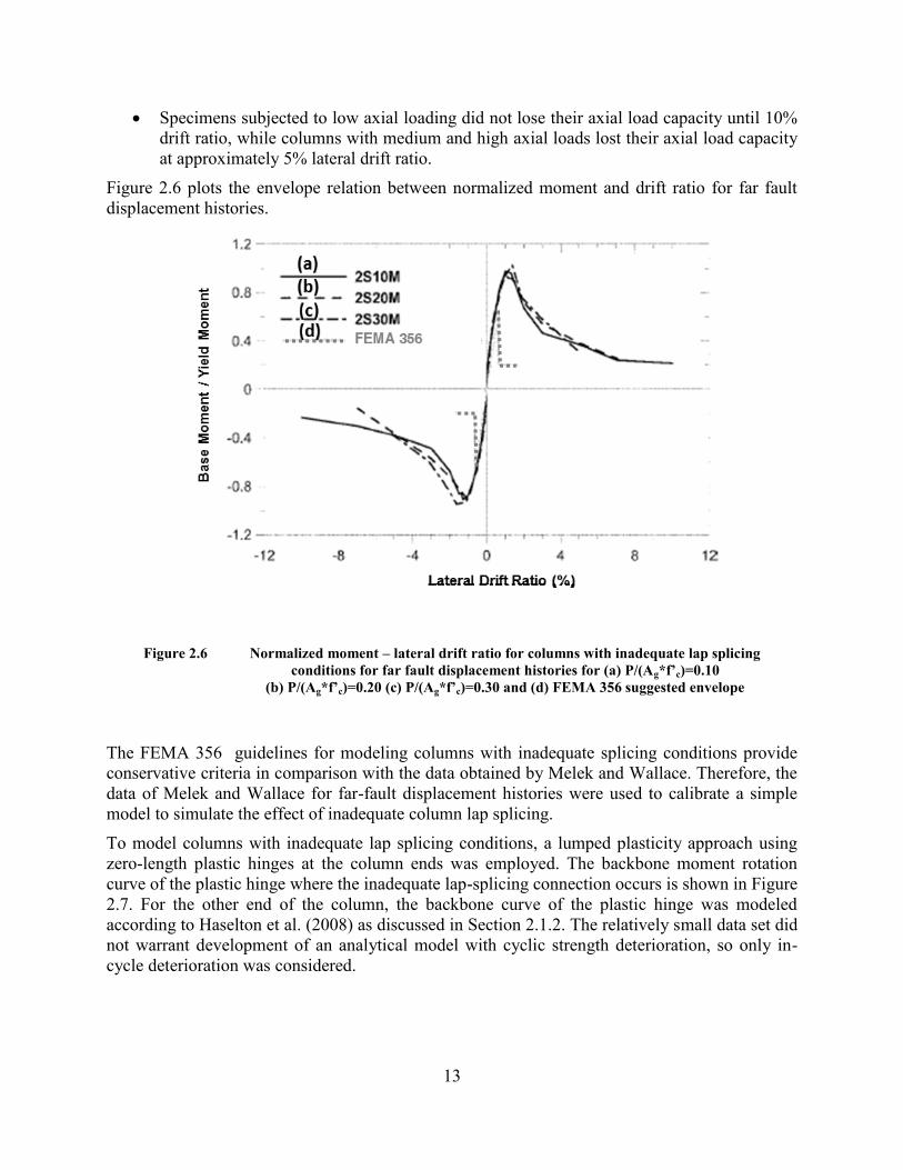
Specimens subjected to low axial loading did not lose their axial load capacity until 10%

drift ratio, while columns with medium and high axial loads lost their axial load capacity

at approximately 5% lateral drift ratio.

Figure 2.6 plots the envelope relation between normalized moment and drift ratio for far fault

displacement histories.

Figure 2.6 Normalized moment – lateral drift ratio for columns with inadequate lap splicing

conditions for far fault displacement histories for (a) P/(Ag*f’c)=0.10

(b) P/(Ag*f’c)=0.20 (c) P/(Ag*f’c)=0.30 and (d) FEMA 356 suggested envelope

The FEMA 356 guidelines for modeling columns with inadequate splicing conditions provide

conservative criteria in comparison with the data obtained by Melek and Wallace. Therefore, the

data of Melek and Wallace for far-fault displacement histories were used to calibrate a simple

model to simulate the effect of inadequate column lap splicing.

To model columns with inadequate lap splicing conditions, a lumped plasticity approach using

zero-length plastic hinges at the column ends was employed. The backbone moment rotation

curve of the plastic hinge where the inadequate lap-splicing connection occurs is shown in Figure

2.7. For the other end of the column, the backbone curve of the plastic hinge was modeled

according to Haselton et al. (2008) as discussed in Section 2.1.2. The relatively small data set did

not warrant development of an analytical model with cyclic strength deterioration, so only in-

cycle deterioration was considered.

14

Figure 2.7 Assumed zero-length plastic hinge rotational behavior for inadequate lap-splicing

conditions

2.1.5 Beam Column Joints for Collapse Simulation

In the current study the beam-column joints are assumed rigid and potential joint failure is not

considered. However, for purpose of completeness, this section presents a brief review of

available models for older-type beam-column joints.

The role of joint failure in the collapse of buildings is a subject of current debate. While it is less

clear whether joints have contributed to vertical load collapse of existing buildings, it seems

irrefutable that joint damage can occur, and this damage can negatively affect the dynamic

response of the building. Most reinforced concrete buildings designed prior to 1970s do not have

joint transverse reinforcement. In such buildings beam-column joint failure could potentially

precede the column shear failure, thereby altering significantly the collapse performance.

Several researchers have proposed analytical models for the shear deformability of joints and for

the slip of reinforcement from the joints. Park and Mosalam (2013) and Hassan and Moehle

(2012) summarize available research and present new models. Both models use the scissors

modeling approach, which consists of a rotational spring connected with rigid links to the beam

and column elements. The rigid links have length equal to the joint dimensions. A schematic

illustration of the joint sub-assemblage is provided in Figure 2.8. The rotational spring located at

the central node could represent either (a) only the shear deformation of the joint (in that case an

extra spring located at the beam column interface could represent the bar slip) or (b) the sum of

the shear deformation of the joint and the joint rotation resulting from bar slip.

0

0.2

0.4

0.6

0.8

1

1.2

0 0.05 0.1

M/M

y

Plastic Rotation (rad)

15

Figure 2.8 Proposed scissors model (Hassan and Moehle, 2012)

Both Park and Mosalam (2013) and Hassan and Moehle (2012) models use a relatively simple

backbone curve to model the joint rotation spring for the corner joints. In Figure 2.9 the model

suggested by Hassan is illustrated, where the corresponding values of shear stress at point 1, 2, 3,

and 4 can be found in Hassan and Moehle (2012).

Joint shear rotational

spring

16

Figure 2.9 Proposed backbone curve of joint shear stress strain (Hassan and Moehle, 2012)

In Figure 2.9, point 1 corresponds to joint cracking, point 2 to pre-peak yielding strength, point 3

is the peak shear strength, and point 4 is the post-peak strength. Point 4 is the maximum drift that

the joint can reach prior to axial failure in case of high axial load ( 3.0'

cg fA

P) or severe joint

distress for the case of low axial load ( 3.0'

cg fA

P).

Hassan suggests the relationship provided in Equation 2.6 to calculate the drift where axial

failure occurs in corner joints.

5.0)*

tan(*057.0)(

fybsb

P

Laxial

(2.6)

where P is the axial load, Asb is the bottom beam reinforcement, fyb is the yield strength, and θ is

the shear crack angle.

Based on tests of corner joints available in the literature, Hassan and Moehle (2013) define a line

that discretizes the axial failure safe zone from the unsafe zone in Figure 2.10. Equation 2.7

describes the analytical expression of the inclined line in Figure 2.10.

gc

axialAf

P

L '72.29

1)(

(2.7)

17

Figure 2.10 Axial load-drift ratio relationship at axial failure for exterior and corner joints

(Hassan 2013)

18

2.2 SEISMIC RISK ASSESSMENT

“Risk assessment is all about risk management. The only reason you do an assessment is because

somebody has to make a risk-management decision” (Smith, 2005).

Quantifying the seismic risk for existing buildings has the benefit of providing information to

building owners or authorities such that informed decisions regarding seismic upgrading can be

made.

Seismic risk has different meanings among different professions or stakeholders. From a

seismological perspective, seismic risk is the probability of earthquakes with specific magnitude

occurring at least once in a specific region during a specified period (Wang, 2006). From a

structural engineering perspective, seismic risk is the probability that a structure will sustain

certain damage at least once in a given period. In the current study we will focus on the latter

definition of seismic risk.

Seismic risk assessment for structural engineering purposes consists of two main procedures:

Seismic Hazard Analysis. This procedure is concerned with estimation of the probability

of exceedance of a certain ground motion parameter or intensity measure during a certain

period of time.

Assessment of Structural Vulnerability. This procedure relates ground motion

intensity with structural response, usually termed as Engineering Demand Parameter

(EDP).

If we define risk as the annual rate of exceedance of a specified EDP level, then risk can be

quantified by using Equation 2.8:

dimdim

)( )|()( |

imIMdimedpGedp

IM

IMEDPEDP

(2.8)

,where EDP corresponds to the Engineering Demand Parameter, IM corresponds to the Intensity

Measure, and GEDP | IM is the complementary cumulative distribution function (CCDF) of an

EDP (e.g., collapse state or a certain story drift rate) given an earthquake Intensity Measure (IM).

Estimating the parameters that define the GEDP | IM is the main objective of the current study.

The estimation of the annual probability of exceedance of a certain earthquake intensity level (in

this study the earthquake intensity level will be defined as spectral acceleration at the

fundamental period of the building) will be assumed to be provided by Probabilistic Seismic

Hazard Analysis (PSHA), which can be performed relatively easily using software available

online provided by USGS or by a specialist in engineering seismology.

In the following sections a review of two approaches commonly used by engineers to estimate

GEDP | IM will be presented.

19

2.2.1 Regress using Unscaled Ground Motions (Cloud Analysis)

According to this method a set of ground motions is selected and then non-linear dynamic

analysis is performed for each unscaled record. Consequently, the results of the analyses are

plotted. Each earthquake corresponds to a dot in a graph that relates EDPs with IMs. The

method is commonly termed as “cloud analysis” because the data as plotted in Figure 2.11a form

an elliptical shape similar to that of a cloud (Baker 2007).

Figure 2.11 Estimating the conditional distribution of EDP | IM at Sa(T1) using “cloud

analysis” (a) conditional mean value from linear regression (b) comparison of strip

of EDP data Gaussian CCDF based on linear regression

(Baker 2007)

This method utilizes simple linear regression to relate IM and EDP through a model described in

Equation 2.9:

)ln( βˆIM)|ln( 10 imβEDP (2.9)

where 0β and 1β are the regression coefficients, IM is the predictor, and ε is the model error.

According to Equation 2.9, for a given IM the )ˆln( PDE prediction is provided. If it is assumed

that variance is constant (homoscedasticity assumption) for all IMs, then the standard deviation

can be estimated as shown in Equation 2.10

20

))ˆln((ln(2

1ˆ 2

i

n

i i PDEEDPn

(2.10)

, where n is the number of simulated analyses. If ln(EDP | IM) is assumed further to have normal

distribution, then GEDP | IM is given by Equation 2.11:

)ˆ

)ln( βˆln(1im)|( 10

IM|

imβedpedpGEDP

(2.11)

, where Φ is the cumulative distribution function of the standard normal distribution.

The assumptions stated above impose restrictions on the applicability of the method.

Specifically, since the variance of EDP is rarely constant at a wide range of IMs, the method

should be applied only for a small range of IM levels.

However, this limitation can be overcome if we apply regression only for limited IM ranges

(such that the regression is piecewise linear). This approach increases the computational effort

and would remove the advantage of the method to provide a closed form solution for Equation

2.11.

2.2.2 Scaling Records to the Target IM Level - IDA

Instead of using unscaled motions having a wide range of IM levels as presented in the previous

section, one can alternatively scale a set of motions so that each matches the IM of interest. At

the IM of interest an empirical cumulative distribution function (ECDF) can be plotted and,

assuming that the EDP follows a certain distribution (e.g., log-normal), we could estimate the

distribution parameters required such that they fit the observed data of the ECDF. According to

this method, IM|EDPG would be estimated according to Equation 2.12.

)ˆ

ˆ)ln((1im)|(IM|

imedpG EDP (2.12)

where and correspond to sample mean and standard deviation.

The procedure can be repeated several times for different IM levels such that multiple stripes of

data are obtained, as shown in Figure 2.12. Interpolation can be used to estimate the probabilities

of exceedance at intermediate IM levels.

This method has the drawback that a large number of dynamic analyses are required to obtain a

large number of stripes. Furthermore, scaling of ground motions is required, which could

21

potentially lead to “artificial,” unrealistic, earthquake motions used in dynamic simulations,

thereby creating a bias in the results. Although the drawbacks of this method seem to be rather

important, the advantage to be able to cover a large range of IM levels makes it appealing. The

latter advantage of the method has made it particularly popular at relatively high IM levels for

which there are not enough available ground motions.

Figure 2.12 Multiple stripes of data for different IM Levels (Baker 2007)

2.2.2.1 Incremental Dynamic Analysis (IDA)

The method presented above can easily be formulated such that it can estimate the probability of

exceedance of EDP at a wide range of IM levels until collapse of the structure. This extension of

the method is called Incremetnal Dynamic Anallysis (IDA) (Vamavatsikos and Cornel, 2002) (or

alternatively dynamic pushover) and involves a series of dynamic non-linear analyses performed

using scaled ground motions whose IM levels are selected and scaled to cover the whole

structural response range from elastic behavior to dynamic instability (collapse).

In the current study, the IDA method was modified such that it focused on estimation of the

probability of collapse, rather than examining the full range of response. The (modified) IDA

procedure is described below.

1. The first step in performing collapse assessment through the IDA concept is selecting

earthquake ground motion records. In the current study a set of 22 pairs of far-field

records (recorded at sites less than 10 km from fault rupture) were selected. The record

22

set that was selected is the same as the set used for the ATC-63 project (FEMA,2009).

The records were selected to meet a number of objectives listed below:

Source Magnitude: Ground motions from large magnitude events (M≥6.5) are selected,

as their longer durations and stronger shaking pose a greater risk for structures.

Source Type: The record set includes ground motions from earthquakes generated from

strike-slip and from thrust fault rupture types. These sources were selected since they

were considered typical of shallow crustal earthquakes in California and other Western

United States locations.

Site Conditions: The records were selected such that they were recorded on different soil

conditions ranging from class B to D (classes A, E, and F were not considered typical for

buildings).

Number of Recordings for each Event: To avoid event-bias, not more than two records

for each event was considered in the record set.

Strong Recordings: To avoid unrealistic scaling of ground motions to achieve structural

collapse, the ground motions were selected such that they possess Peak Ground

Acceleration (PGA) > 0.2g and Peak Ground Velocity (PGV) > 15cm/sec. These values

were considered the thresholds of earthquakes that could cause structural damage.

Recording Location: To avoid soil-structure-foundation interaction, recordings from

instruments located in free-field or ground floor of small buildings were used.

Tables 2.1 and 2.2 summarize the record set ground motion characteristics used in the current

study.

23

Table 2.1 Far-field record set used in the current study

ID No. Earthquake Recording Station

M Year Name Name Owner

1 6.7 1994 Northridge Beverly Hills- Mulljol USC

2 6.7 1994 Northridge Canyon Country- WLC USC

3 7.1 1999 Duzce, Turkey Bolu ERD

4 7.1 1999 Hector Mine Hector SCSN

5 6.5 1979 Imperial Valley Delta UNAMUCSD

6 6.5 1979 Imperial Valley El Centro Array #11 USGS

7 6.9 1995 Kobe, Japan Nishi- Akashi CUE

8 6.9 1995 Kobe, Japan Shin-Osaka CUE

9 7.5 1999 Kocaeli, Turkey Duzce ERD

10 7.5 1999 Kocaeli, Turkey Arcelik CDMG

11 7.3 1992 Landers Yermo Fire Station KOERI

12 7.3 1992 Landers Coolwater SCE

13 6.9 1989 Loma Prieta Capitola CDMG

14 6.9 1989 Loma Prieta Gilroy Array #3 CDMG

15 7.4 1990 Manji, Iran Abbar BHRC

16 6.5 1987 Superstition Hills El Centro Imp. Co CDMG

17 6.5 1987 Superstition Hills Poe Road (temp) USGS

18 7.0 1992 Cape Mendocino Rio Dell Overpass CDMG

19 7.6 1999 Chi-Chi Taiwan CHY101 CWB

20 7.6 1999 Chi-Chi Taiwan TCU045LA CWB

21 6.6 1971 San Fernando LA - Hollywood Stor CDMG

22 6.5 1976 Friuli, taly Tolmezzo ..

24

Table 2.2 Far-field ground motion parameter information

ID No.

PEER-NGA Record Information Recorded Motions

File Names - Horizontal Records PGAmax PGVmax

Component 1 Component 2 (g) (cm/s)

1 NORTHR/MUL009 NORTHR/MUL279 0.52 63

2 NORTR/LOS000 NORTR/LOS270 0.38 45

3 DUZCE/BOL000 DUZCE/BOL090 0.82 62

4 HECTOR/HEC000 HECTOR/HEC090 0.34 42

5 IMPVALL/H-DLT262 IMPVALL/H-DLT352 0.35 33

6 IMPVALL/H-E11140 IMPVALL/H-E11230 0.38 42

7 KOBE/NIS000 KOBE/NIS090 0.51 37

8 KOBE/SHI000 KOBE/SHI090 0.24 38

9 KOCAELI/DZC180 KOCAELI/DZC270 0.36 59

10 KOCAELI/ARC000 KOCAELI/ARC090 0.22 40

11 LANDERS/YER270 LANDERS/YER360 0.24 52

12 LANDERS/CLW-LN LANDERS/CLW-TR 0.42 42

13 LOMAP/CAP000 LOMAP/CAP090 0.53 35

14 LOMAP/G03000 LOMAP/G03090 0.56 45

15 MANJIL/ABBAR-L MANJIL/ABBAR-T 0.51 54

16 SUPERST/B-ICC000 SUPERST/B-ICC090 0.36 46

17 SUPERST/B-POE270 SUPERST/B-POE360 0.45 36

18 CAPEMEND/RIO270 CAPEMEND/RIO360 0.55 44

19 CHICHI/CHY101E CHICHI/CHY101N 0.44 115

20 CHICHI/TCU045-E CHICHI/TCU045-N 0.51 39

21 SFERN/PEL090 SFERN/PEL180 0.21 19

22 FRIULI/A-TMZ000 FRIULI/A-TMZ270 0.35 31

2. The second step in the procedure corresponds to gradual scaling of each ground motion

until the structure leads to collapse. For each ground motion analysis the maximum story

drift ratio and corresponding Sa(T1) level are reported as a dot in Figure 2.13(a).

Consequently the dots for each ground motion are connected by lines (assuming linear

interpolation between Sa(T1) and maximum story drift ratio). These lines are termed as

the IDA curves and correspond to a dynamic pushover for each record. In Figure 2.13(a),

a total of 44 lines are shown (equal to the number of total records used).

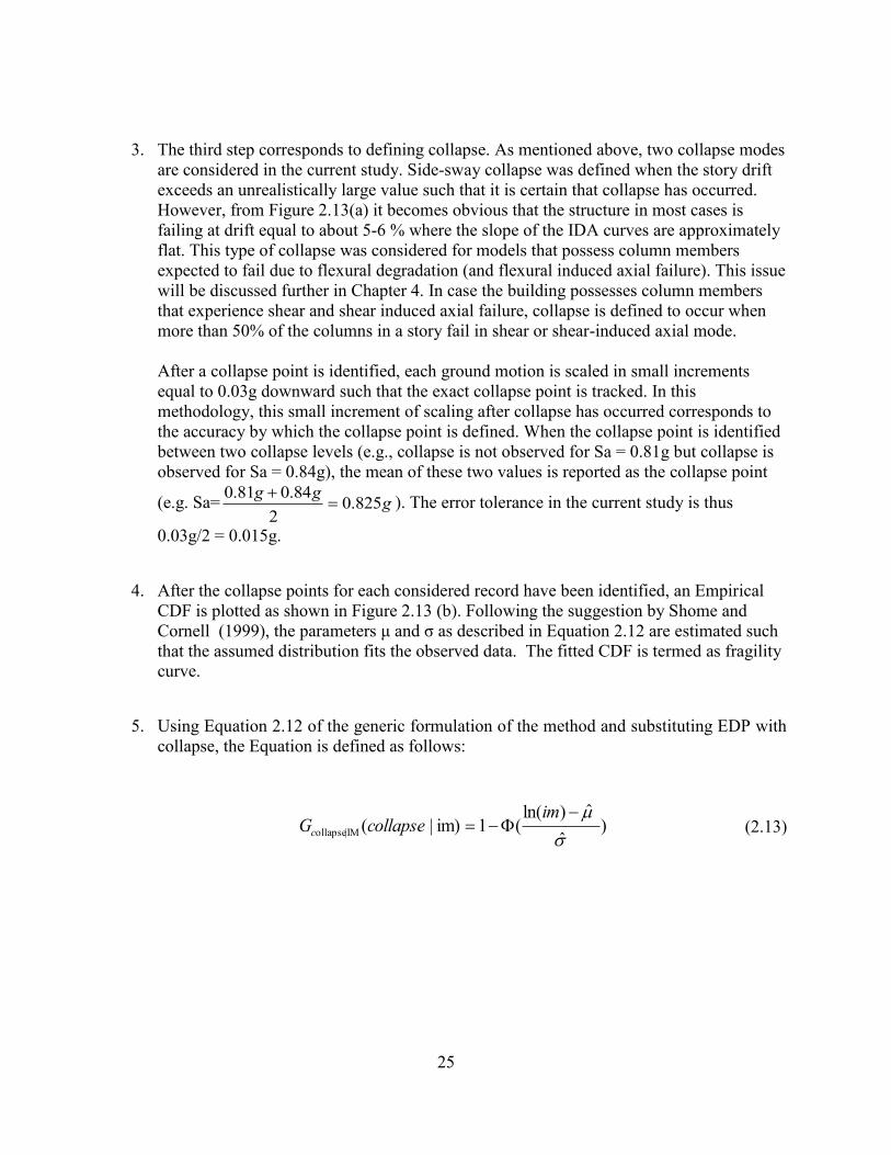
25

3. The third step corresponds to defining collapse. As mentioned above, two collapse modes

are considered in the current study. Side-sway collapse was defined when the story drift

exceeds an unrealistically large value such that it is certain that collapse has occurred.

However, from Figure 2.13(a) it becomes obvious that the structure in most cases is

failing at drift equal to about 5-6 % where the slope of the IDA curves are approximately

flat. This type of collapse was considered for models that possess column members

expected to fail due to flexural degradation (and flexural induced axial failure). This issue

will be discussed further in Chapter 4. In case the building possesses column members

that experience shear and shear induced axial failure, collapse is defined to occur when

more than 50% of the columns in a story fail in shear or shear-induced axial mode.

After a collapse point is identified, each ground motion is scaled in small increments

equal to 0.03g downward such that the exact collapse point is tracked. In this

methodology, this small increment of scaling after collapse has occurred corresponds to

the accuracy by which the collapse point is defined. When the collapse point is identified

between two collapse levels (e.g., collapse is not observed for Sa = 0.81g but collapse is

observed for Sa = 0.84g), the mean of these two values is reported as the collapse point

(e.g. Sa= ggg

825.02

84.081.0

). The error tolerance in the current study is thus

0.03g/2 = 0.015g.

4. After the collapse points for each considered record have been identified, an Empirical

CDF is plotted as shown in Figure 2.13 (b). Following the suggestion by Shome and

Cornell (1999), the parameters μ and σ as described in Equation 2.12 are estimated such

that the assumed distribution fits the observed data. The fitted CDF is termed as fragility

curve.

5. Using Equation 2.12 of the generic formulation of the method and substituting EDP with

collapse, the Equation is defined as follows:

)ˆ

ˆ)ln((1im)|(IM|ollapse

imcollapseGc (2.13)

26

Figure 2.13 Development of fragility curves: (a) IDA curves for an 8-story building,

(b) Derived fragility Curve for an 8-story building

2.3 IDENTIFYING PARAMETERS INFLUENCING THE COLLAPSE

PERFORMANCE

As explained in Chapter 1, buildings designed prior to 1980s suffer from several structural

deficiencies, mainly due to proportioning that creates a weak story or due to lack of appropriate

seismic detailing. As part of the NEES Grand Challenge Program, in the NIST Program Plan, a

list of critical deficiencies that according to engineers in practice have a significant influence to

the collapse vulnerability of older-type concrete buildings was provided. The list is shown in

Table 2.3

27

Table 2.3 Critical seismic deficiencies found in pre-1980 concrete buildings (NIST GCR 10-917-7)

In the NIST program plan, it was suggested to link the deficiencies presented in Table 2.3 with

simple engineering parameters. These parameters should not require any complicated analysis,

but instead should be easy to calculate based on information obtained by reviewing the structural

drawings. The program plan suggested that any of the parameters that according to analysis is

28

shown to be highly correlated with collapse performance of the structure could be termed a

“collapse indicator.”

In Chapter 5, following directly the approach suggested by NIST, it was verified that certain

parameters such as the column to beam bending moment strength ratio are highly correlated to

collapse performance. The approach that was followed corresponds to varying the values of one

parameter and accordingly obtaining the corresponding fragility curve of the building as depicted

in Figure 2.14. It was shown that there is a critical point where further increase or decrease in the

value of the parameter results in dramatic change of probability of collapse.

Figure 2.14 Approach for establishing collapse indicator limits. Example collapse fragilities for

different collapse indicator values (ΣΜnc/ΣΜnb: column to beam bending moment

strength ratio, IM: Earthquake Intensity Measure)

2.4 ESTIMATING STORY DRIFT DEMAND

The current study uses a large number of dynamic analyses performed through the IDA method

to provide regression estimates regarding drift demands.

A similar approach was followed by Shome and Cornell (1999) to estimate maximum story drift

ratio demands. In his study, Shome employed two structural steel, special moment resisting

frames (SMRFs) designed according to the LRFD specifications (LRFD,1994). To estimate story

drift ratio demand Shome tried to perform statistical regression based on numerous non-linear

dynamic analyses using scaled ground motions. Figures 2.15 and 2.16 depict the considered

buildings:

IM

Pcol

(ΣΜnc/ΣΜnb)=1.20

(ΣΜnc

/ΣΜnb

)=0.80

(ΣΜnc/ΣΜnb)IMmce (ΣΜnc/ΣΜnb)limit

Pcol

“good”

building

fragility

29

Figure 2.15 5-story SMRF (Shome, 1999)

Figure 2.16 20-story SMRF (Gupta, 1999)

In his study Shome relates the maximum story drift with different intensity parameters using

regression. The results of linear regression for both the 5 and 20 story building are cited below:

30

Table 2.4 Regression relationships of maximum story drift and different intensity measures

(Shome, 1999)

Building Predictor(s) Regressions Fuction R2 σln,ε

5-Story

Sa(T1) DR=0.03*Sa(T1)1.00 0.76 0.38

Sa(T2), Sa(T1) DR=0.02*Sa(T1)0.75*Sa(T2)

0.25 0.8 0.35

Sa(T1) , M DR=0.01(Sa(T1)1.00* e0.13M 0.77 0.37

Sa(T1), R DR=0.02*Sa(T1)1.00*R0.11 0.76 0.37

Sa(T1) , D DR=0.03*Sa(T1)1.00* e0.003D 0.76 0.38

20-Story

Sa(T1) DR=0.16*Sa(T1)0.95 0.7 0.44

Sa(T1), Sa(T2) DR=0.09*Sa(T1)0.56*Sa(T2)

0.40 0.8 0.36

Sa(T1) , M DR=0.01(Sa(T1)0.53* e-0.08M 0.71 0.44

Sa(T1), R DR=0.32*Sa(T1)0.95*R-0.22 0.72 0.43

Sa(T1) , D DR=0.19*Sa(T1)0.95* e0.01D 0.71 0.43

Where, Sa(T1) (g) is the ground motion spectral acceleration at the 1st mode period, Sa(T2) (g) is

the ground motion spectral acceleration at the 2nd

mode period, M corresponds to the earthquake

magnitude, R is the epicentral distance, and D is the ground motion duration.

To derive the regression functions shown in Table 2.4 Shome assumed different linear regression

models with the general formulation presented in Equation 2.14

....)ln( β)1ln( βˆ,...)IM,IM|ln( 221021 imimβIDR (2.14)

The regression estimates demonstrated that for the 5-story building, Sa(T1) is the most

statistically significant parameter while Sa(T2), M, R, and D did not seem to influence so much

the results. In contrast, for the 20-story building both Sa(T1) and Sa(T2) are significant, which

can be observed by the significant reduction in the error of the model that includes both Sa(T1)

and Sa(T2). This observation is intuitive since for the taller building higher modes are expected

to be more significant. The relatively high R2 values demonstrate that the regression model

largely explains the variability in the maximum story drift.

In Table 2.4, for the regression function with Sa(T1) being the only predictor to estimate

maximum story drift, 1β1 for both the 5 and 20-story buildings. This implies that the maximum

story drift (DR) is an approximately linear function of Sa(T1).

31

Based on the assumption that there is an approximately linear relationship between DR and

Sa(T1) as demonstrated by Shome and Cornell (or in other words that β1=1.0), Equation 2.14 can

be simplified to Equation 2.15, which is more intuitive for engineers. The latter equation implies

a linear relationship between the predicted maximum story drift demand ΔD and the average drift

ratio δeff/heff.

)/ln(ˆ)IM|ln( 01 effeffD hβ (2.15)

, where ΔD corresponds to the predicted story drift demand, δeff is the displacement at the

effective height of the building (δeff is a function of Sa(T1)), and heff is the effective height of the

building assumed to be equal to 70% of the total building height.

Equation 2.15 was used in the current study to relate story drift demand and average drift ratio.

The relationship 2.15 was calibrated using results from the non-linear dynamic analysis

performed as part of the IDA. The calibration was performed such that the estimated coefficient

0β minimizes the sum of the square errors.

If we define α=exp ( 0β ) in Equation 2.15, then α links linearly the average drift ratio and the

predicted maximum story drift (ΔD=α*δeff/heff). This procedure will be discussed further in

Chapter 6 and Appendix G.

The regression results obtained in the current study using IDA agree with those estimated by

Shome and Cornell. In the current study the goodness of fit of Equation 2.15 was checked

visually. Further research is required to determine a model that would relate story drift ratio

demand with intensity measures in an optimal way such that both simplicity and high accuracy

are satisfied.

2.5 ESTIMATING COLUMN DRIFT CAPACITY

After the drift demand has been defined using the procedure described above, the current

methodology requires estimation of the column drift capacity. In the current study, drift capacity

is defined deterministically using the shear failure surface suggested by Elwood, as expressed by

Equation 2.1 at the beginning of this chapter.

In the general formulation of the methodology, capacity can also be defined as random variable

taking into account material and modeling uncertainties, but that approach was not pursued here.

Liel et al. (ATC-78, 2014) defined column deformation capacity in terms of column base

rotation. The approach suggested by Liel attempts to follow the same procedure used by ASCE

41 to define component deformation capacities.

Following the ASCE 41 procedure, Liel suggests that columns should be classified according to

their structural detailing using Table 2.5

32

Table 2.5 Classification of column condition (Li et al. 2013)

Transverse Reinforcement Details

ACI conforming details with 135° hooks

Closed hoops with 90°

hooks

Other (including lap

spliced transverse

reinforcement)

Ratio of flexural to

shear strength

(Vp/Vn) ≤0.6 i ii ii

1.1 ≥ (Vp/Vn) ≥ 0.6 ii ii iii

(Vp/Vn) > 1.1 iii iii iii

Based on linear regression of experimental results by Berry et al. (2004), Liel defines in Table

2.6 column deformation capacities that correspond to column axial failure level. The column

deformation capacities defined by Liel could be compared with parameter b of the ASCE-41

backbone curve for column force-deformation response. The ASCE-41 backbone curve for

component force-deformation response is presented in Figure 2.17. Table 2.7 presents a

comparison between column deformation capacities as suggested by Liel et al. (2014) and

ASCE-41

Figure 2.17 Backbone curve of component force-deformation response in ASCE-41

(Li et al. , 2013)

33

Table 2.6 Column deformation capacities according to column condition (Liel et al. 2014)

P/Agf’c ρv = Av/bws Plastic Rotation Capacity c

Condition i

≤ 0.1 ≥ 0.006 0.090

≥ 0.6 ≥ 0.006 0.030

≤ 0.1 = 0.002 0.050

≥ 0.6 = 0.002 0.018

Condition ii

≤ 0.1 ≥ 0.006 0.082

≥ 0.6 ≥ 0.006 0.023

≤ 0.1 ≤ 0.0005 0.025

≥ 0.6 ≤ 0.0005 0.011

Condition iii

≤ 0.1 ≥ 0.006 0.075

≥ 0.6 ≥ 0.006 0.020

≤ 0.1 ≤ 0.0005 0.016

≥ 0.6 ≤ 0.0005 0.006

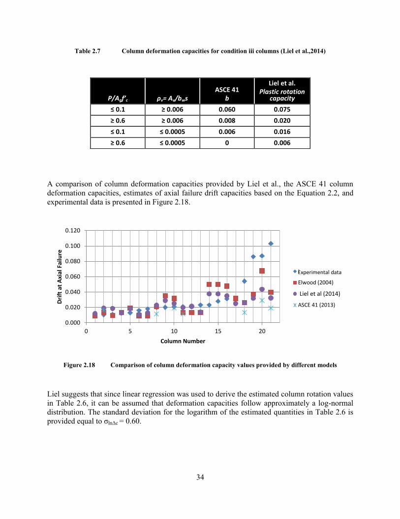
34

Table 2.7 Column deformation capacities for condition iii columns (Liel et al.,2014)

A comparison of column deformation capacities provided by Liel et al., the ASCE 41 column

deformation capacities, estimates of axial failure drift capacities based on the Equation 2.2, and

experimental data is presented in Figure 2.18.

Figure 2.18 Comparison of column deformation capacity values provided by different models

Liel suggests that since linear regression was used to derive the estimated column rotation values

in Table 2.6, it can be assumed that deformation capacities follow approximately a log-normal

distribution. The standard deviation for the logarithm of the estimated quantities in Table 2.6 is

provided equal to σlnΔc = 0.60.

0.000

0.020

0.040

0.060

0.080

0.100

0.120

0 5 10 15 20

Dri

ft a

t A

xial

Fai

lure

Column Number

Empirical

Elwood (2004)

This methodology

ASCE 41 (2013)

Experimental data

Liel et al (2014)

P/Agf’c ρv= Av/bws ASCE 41

b

Liel et al. Plastic rotation

capacity

≤ 0.1 ≥ 0.006 0.060 0.075

≥ 0.6 ≥ 0.006 0.008 0.020

≤ 0.1 ≤ 0.0005 0.006 0.016

≥ 0.6 ≤ 0.0005 0 0.006

35

Assuming a log-normal distribution for the column deformation capacity values provided above

and a log-normal distribution for the story drift demand values as discussed in the previous

section, the probability that demand will exceed capacity can be calculated by Equations 2.16 –

2.17:

xC

xC

ln,2

ln,2

ln,ln,

(Eq. 2.16)

)())ln()(ln( CDP (Eq. 2.17)

36

3 Evaluation of Collapse Simulation of Concrete

Frame Structures

Later chapters of this report will use non-linear dynamic analyses to evaluate the seismic

performance of buildings. Modeling the non-linear response and more specifically brittle failure

modes like shear and shear-induced axial failure that existing concrete buildings are susceptible

to, is a particularly challenging task. Most of the models available in the literature have been

calibrated by results of pseudo-static laboratory test, in which the tested column is subjected to

displacement reversals of increasing amplitude until substantial loss of strength. As suggested in

Haselton et al (2008), tests with a greater variety of loading histories are required to improve the

accuracy of the current modeling techniques.

In this Chapter, the results of eleven one-story, one-bay reinforced concrete test structures

subjected to base motions on a shaking table are presented. The columns in the test structures

had either widely spaced transverse reinforcement or closely spaced transverse reinforcement

resulting in relatively brittle or relatively ductile response. The base motions represented either a

long-duration motion without significant long-period pulses or a shorter duration motion with a

significant velocity pulse, imparted with an intensity that caused collapse of the test structures.

Analytical models of the test structures were developed for the purpose of exploring the

simulation capabilities that have been used in this study to evaluate the performance of existing

buildings.

In the sections below a brief overview of the experimental setup and material properties is

provided. Consequently a comparison between results obtained by using collapse simulation

analytical tools with those obtained from the actual laboratory tests is presented. The interested

reader can find further details about the presented laboratory tests in Shin (2007).

3.1 EXPERIMENTAL INVESTIGATION

A laboratory test program was designed to test reinforced concrete columns subjected to

dynamic lateral loading. The purpose of the test program was to investigate the dynamic

response of column members with different ductility. Two different types of columns were

tested. The first type had dense spacing of transverse reinforcement, similar to requirements of

current code provisions for buildings in regions of high seismicity. This column type was

intended to have a ductile load-displacement response. The second type had wide spacing of

transverse reinforcement, characteristic of building practices prior to 1970s. This column type

was intended to yield in flexure, followed by shear and axial failure. Fig. 3.1 illustrates the two

37

column types. Due to limitations of the shaking table, the scale of the test columns was

approximately one-third of their full scale. Normal-weight concrete compressive strength ranged

from 3 to 4 ksi. Longitudinal reinforcement was Grade 60.

For the shear-critical columns, the geometry by Lynn (1996) and Sezen (2002) was chosen as the

prototype. The full-scale prototype column had a 18” square column with a net height equal to

9’-8”. Eight #9 longitudinal bars were spaced evenly around the column perimeter with #3 ties

with 12" spacing. The one-third scaled shear-critical columns consisted of a 6” square column

with eight #3 longitudinal reinforcing bars spaced evenly around the column perimeter with a

cover of equal to 2/3” (longitudinal reinforcement ratio equal to 2.44%). The longitudinal bars

were embedded in a top and bottom beam stub. The bars were bent with 90-degree hooks of

length 12db (where db is the longitudinal bar diameter) to prevent pullout failure. Plain 1/8”

diameter wire was used for the transverse reinforcement. The transverse reinforcement consisted

of a perimeter hoop plus two crossties (one in each direction). Hoops had 90-degree anchorage

hook with length equal to 6db. Crossties had 90-degree hook on one end and 135-degree hook on

the other end. The transverse reinforcement was spaced at 4” center-to-center distance along the

column height with the 90-degree hook crossties alternated along the height.

The ductile columns had the same gross dimensions with the same longitudinal reinforcement

configuration as the shear-critical columns. The only difference between the two column types

was the transverse reinforcement detailing. The transverse reinforcement details of the ductile

columns were designed to comply with the ACI 318. For the ductile columns, (3/16)” diameter

plain wire was used as transverse reinforcement with center-to-center spacing equal to 1-1/2”

along the length of the column. The transverse reinforcement consisted of hoops with 135-degree

hooks with anchorage length equal to 6db and of crossties with 135-degree hooks as well.

The single-bay frame that is shown in Fig. 3.2 was selected for the test series. Since the purpose

of the test was to understand the non-linear dynamic behavior of columns, an idealized, re-

usable, nearly-rigid steel beam was used to connect and load the two concrete columns of a test

frame. The base of the columns was supported by a nearly rigid load cell that connected to the

stiff shaking table, creating a nearly-fixed base for the test frames. In the event of column axial

failure, a pin-ended steel column was provided to catch the test structure and enable the test to

proceed without total system vertical collapse. Axial load and inertial load were provided by lead

ingots fixed to the steel beam. This resulted in at rest axial load of 0.1*Ag*f’c. Additional axial

load, producing a total axial force equal to 0.24*Ag*f’c was achieved in some of the tests by

using a pneumatic jacking system, testing the sensitivity of dynamic response to axial loading.

At beam-column joints, the tie configurations had ductile details according to the ACI 318 code

provisions (hoops with 38 mm spacing distance and 135 degree hooks for hoops and crossties

alternated along the height of the joint) for both the ductile and the non-ductile specimens.

To achieve different frame response characteristics, the columns were combined in three

different ways, that is, a combination of two ductile columns, two non-ductile columns, or one

ductile column and one non-ductile column. Table 3.1 summarizes the combinations used for the

test series.

38

Figure 3.1 Reinforced concrete column specimen details:

(a) Non-ductile column (b) Ductile column

Figure 3.2 Experimental setup

39

Table 3.1 Test matrix

Test Number Column Combination Ground Motion Axial Load Ratio

(P/Ag*f’c)

1 Duct. - NonDuct. Chile 0.10

2 Duct. - NonDuct. Kobe 0.10

3 Duct. - Duct. Chile 0.10

4 NonDuct. - NonDuct. Chile 0.10

5 Duct. -Duct. Kobe 0.10

6 NonDuct. - NonDuct. Kobe 0.10

7 Duct. - NonDuct. Chile 0.24

8 Duct. - NonDuct. Kobe 0.24

9 Duct. - Duct. Chile 0.24

10 NonDuct. - NonDuct. Chile 0.24

11 Duct. -Duct. Kobe 0.24

121 NonDuct. - NonDuct. Kobe 0.24

3.2 INPUT GROUND MOTIONS

To understand how different types of ground motions can influence the dynamic response, two

different unidirectional ground motion records were considered (out-of-plane motion was

restrained by using a bracing mechanism). These were the ground motion recorded at Llolleo

100-degree component during the 1985 Chile earthquake (long-duration motion without

significant long-period pulses) (Fig. 3.3); and the ground motion recorded at JMP station in the

North-South direction during the 1995 Kobe Earthquake (shorter duration motion with a

significant velocity pulse) (Fig. 3.4).

The ground motions were scaled so that they are consistent with the one-third scale similitude

requirements by multiplying the duration of the ground motion by a factor of 1/ 3 . The

intensities of the ground motions were scaled to achieve the targeted responses; more specifically

the amplitude of Llolleo input motion was scaled by a factor of 3.2 and the amplitude of Kobe

input motion was scaled by a factor of 1.35. The ground motions were filtered by removing high

and low frequencies to meet the shaking table limits.

1 Data from this test were missing; the results from test 12 are not presented in the current study

40

Figure 3.3 Filtered Llolleo input ground motion (Chile 1985) ;

(a) Ground motion , (b) Linear response spectrum (2% damping ratio)

Figure 3.4 Filtered Kobe Input Ground Motion (Kobe 1995):

(a) Ground motion, (b) Linear response spectrum (2% damping ratio)

(b)

_a

Sa (

g)

Acc

eler

ati

on

(g)

Time (sec)

Period (sec)

Sa (

g)

Acc

eler

ati

on

(g)

Time (sec)

Period (sec)

(a)

_a

(a)

_a

(b)

_a

41

3.3 MATERIAL PROPERTIES

Concrete had normal weight aggregates with specified nominal compressive strength equal to 3

ksi. The column specimens were cast in three groups. Concrete cylinders were cast and cured

along with the specimens of each group. Table 3.2 lists the mean compressive and tensile

strength values of the concrete specimens.

The longitudinal bars were specified as Grade 60 ASTM A706. Three samples of the #3 bars

were tested to obtain the mean yield (fy) and ultimate strength values (fu) .The wires were also

tested to obtain mean strength properties. The results of the steel coupon tests are summarized in

Table 3.3.

Table 3.2 Concrete mean strength properties

Batch Mean Compressive

Strength (ksi) Mean Tensile Strength

(ksi)

1 3.37 0.31

2 4.02 0.40

3 3.74 0.38

Table 3.3 Steel reinforcement mean strength properties

Steel Reinforcement Yield Stress

fy (ksi) Ultimate Stress

fu (ksi)

#3 (long. bars) 64.4 84.7

1/8" wire (transv. reinf.) 80.4 96.1

3/16" wire (transv. reinf.) 79.6 87.0

42

3.4 COMPARISON OF ANALYTICAL MODELS WITH TEST RESULTS

As mentioned at the beginning of this chapter, modeling the collapse behavior of non-ductile

concrete specimens is a challenging task due to the brittle nature of their failure. In this section

the results obtained from the laboratory tests are compared with those obtained from simulation

of the frames using state-of-the-art collapse simulation tools. The results are discussed in term of

lateral displacement at the top of the column and moment at the base of the column. Verification

of the accuracy of different collapse simulation analytical tools used in the current study is

essential for model calibration and for providing a measure of the accuracy of the collapse

evaluation performed in Chapters 5 and 6.

A variety of different analytical models have been developed for dynamic simulation of the non-

linear behavior of structural elements. The models used in the current study are proposed by

Haselton et al. (2008)2 and Elwood and Moehle (2002)3. Both of these models are implemented

in OpenSees structural analysis software. The Elwood model was originally developed

specifically for flexure-shear critical column members so it will be used to simulate only the

response of non-ductile column members, while the Haselton model was developed to address a

wider range of structural components, so it will be used to simulate the response of both ductile

and non-ductile members.

As explained in Chapter 2 the Haselton model represents the column using a lumped plasticity

approach comprising nonlinear springs at the column ends interconnected by a linear-elastic

element. The nonlinear rotational spring behavior was based on the Clough model, using

hysteresis implemented in OpenSees by Ibarra et al. (2005) with stiffness and strength

degradation determined by parameters defined in Haselton et al. (2007). The Elwood model uses

a similar approach, but adds a horizontal and axial spring to represent nonlinear shear and axial

response.

The tested concrete frames were analyzed using the same procedure used in the following

chapters to evaluate the collapse performance of buildings. The stiffness properties of the

structural components were calculated according to ASCE 41-06, the strength values were

calculated by moment-curvature analysis using software XTRACT, and the parameters related

to non-linear deformation and strength degrading behavior were estimated according to the

models proposed by Haselton and Elwood, respectively, with the following exceptions:

As discussed in Chapter 2, the original Haselton model was calibrated using a database

(Berry et al., 2004) including both ductile and non-ductile column members. For the

purposes of the current study the relationships that define the modeling parameters for the

ductile column members were re-calibrated by Dr. Liel and her colleagues such that

columns sustaining apparent shear failures were excluded from the data (ATC-78, 2013).

For the non-ductile column members the parameters were defined according to the

original modeling parameters as suggested by Haselton et al. (2008). The interested

reader can find both the original and the re-calibrated relationships that are used to

calculate the column modeling parameters in Appendix B.

As explained in Chapter 2, Elwood model was not intended originally to be capture shear

failure when it preceded flexural yielding. Elwood model in this study was modified by

2 For brevity this model will be referred as the Haselton model in the current study

3 For brevity this model will be referred as the Elwood model in the current study

43

the author such that if the shear demand exceeds the shear strength as defined according

to ASCE-41-06 (2006) then shear failure is triggered. Also, in this Chapter the axial

spring used to track shear-induced axial failure was not utilized, so the column axial

response was not modeled explicitly.

The values of the modeling parameters used for all the frame combinations are provided in

Tables 3.4 – 3.6 .

Table 3.4 Column modeling properties

Column v (Paxial/Ag*f'c) Yield Strength

My (kip-in) Ultimate Strength

Mu (kip-in) Cracked Stiffness

Factor (per ASCE-41)

Ductile 0.11 137.42 164.9 0.300

Ductile 0.24 150.00 180.0 0.440

Non-Ductile 0.11 137.42 164.9 0.300

Non-Ductile 0.24 150.00 180.0 0.440

Table 3.5 Modeling parameters (Haselton model)

Haselton

Column v (Paxial/Ag*f'c) Plastic Rotation

(θpl) Post Capping Rotation (θpc)

Deterioration Rate Parameter λ

Residual Strength

Ductile 0.11 0.08 0.1000 87 0.1

Ductile 0.24 0.072 0.1000 74 0.1

Non-Ductile 0.11 0.029 0.0440 27 0.1

Non-Ductile 0.24 0.023 0.0300 23 0.1

44

Table 3.6 Modeling parameters (Elwood model)

Column v (Paxial/Ag*f'c) Concrete

Strength f'c (ksi)

Transverse Reinf. Ratio

ρtransverse

Ductile - - -

Ductile - - -

Non-Ductile 0.11 3.7 0.0015

Non-Ductile 0.24 3.7 0.0015

Geometric nonlinearities were considered using the P-Delta formulation. Rayleigh damping was

employed, with coefficients selected to achieve a damping ratio of 2% at the observed

fundamental period of each test (approximately equal to 0.20 sec) and 0.02 sec (this value

corresponds to the second mode period estimated from eigenvalue analysis of the concrete

frames).

The actual period and damping ratio of the test frame were determined from free-vibration tests

conducted prior to earthquake simulation. Table 3.7 summarizes the average period and damping

ratios for the entire test series.

45

Table 3.7 Fundamental Period and damping ratio

Test T (sec) Damping

Ratio ζ (%)

Analytical Model

0.18 2

1 0.22 2.9

2 0.22 2.6

3 0.22 2.8

4 0.23 2.9

5 0.23 2.7

6 0.21 2.5

7 0.18 1.4

8 0.18 1.5

9 0.2 1.6

10 0.2 1.6

11 0.19 1.5

Figures 3.5 to 3.15 compare measured and calculated responses using the Haselton model.

46

Figure 3.5 Comparison of test 1 results with the Haselton model

Figure 3.6 Comparison of Test 2 results with the Haselton model

0 10 20 30 40 50 60 70-6

-4

-2

0

2

4

6

Time (sec)

Dis

pla

ce

me

nt

(in

)Top Column Displacement

Analysis

Test 1

-0.15 -0.1 -0.05 0 0.05 0.1 0.15-200

-150

-100

-50

0

50

100

150

200Column 1

Drift / Height

Ba

se

Mo

me

nt

(kip

s-i

n)

-0.15 -0.1 -0.05 0 0.05 0.1 0.15-200

-150

-100

-50

0

50

100

150

200Column 2

Drift / Height

Ba

se

Mo

me

nt

(kip

s-i

n)

0 10 20 30 40-6

-4

-2

0

2

4

6

Time (sec)

Dis

pla

ce

me

nt (i

n)

Top Column Displacement

Analysis

Test 2

-0.1 -0.05 0 0.05 0.1-200

-150

-100

-50

0

50

100

150

200Column 1

Drift / Height

Ba

se

Mo

me

nt (k

ips-i

n)

-0.15 -0.1 -0.05 0 0.05 0.1 0.15-200

-150

-100

-50

0

50

100

150

200Column 2

Drift / Height

Ba

se

Mo

me

nt

(kip

s-i

n)

47



0 10 20 30 40 50 60 70-6

-4

-2

0

2

4

6

Time (sec)

Dis

pla

ce

me

nt

(in


Analysis

Test 3

-0.15 -0.1 -0.05 0 0.05 0.1 0.15-200

-150

-100

-50

0

50

100

150

200Column 1

Drift / Height

Ba

se

Mo

me

nt

(kip

s-i

n)

-0.15 -0.1 -0.05 0 0.05 0.1 0.15-200

-150

-100

-50

0

50

100

150

200Column 2

Drift / Height

Ba

se

Mo

me

nt

(kip

s-i

n)

0 10 20 30 40 50 60 70-10

-8

-6

-4

-2

0

2

4

6

Time (sec)

Dis

pla

ce

me

nt

(in

)


Analysis

Test 4

-0.15 -0.1 -0.05 0 0.05 0.1 0.15-200

-150

-100

-50

0

50

100

150

200Column 1

Drift / Height

Ba

se

Mo

me

nt

(kip

s-i

n)

-0.15 -0.1 -0.05 0 0.05 0.1 0.15-200

-150

-100

-50

0

50

100

150

200Column 2

Drift / Height

Ba

se

Mo

me

nt

(kip

s-i

n)

48



0 10 20 30 40-6

-4

-2

0

2

4

6

Time (sec)

Dis

pla

ce

me

nt

(in


Analysis

Test 5

-0.15 -0.1 -0.05 0 0.05 0.1 0.15-200

-150

-100

-50

0

50

100

150

200Column 1

Drift / Height

Ba

se

Mo

me

nt

(kip

s-i

n)

-0.15 -0.1 -0.05 0 0.05 0.1 0.15-200

-150

-100

-50

0

50

100

150

200Column 2

Drift / Height

Ba

se

Mo

me

nt

(kip

s-i

n)

0 10 20 30 40-6

-4

-2

0

2

4

6

Time (sec)

Dis

pla

ce

me

nt

(in

)


Analysis

Test 6

-0.15 -0.1 -0.05 0 0.05 0.1 0.15-200

-150

-100

-50

0

50

100

150

200Column 1

Drift / Height

Ba

se

Mo

me

nt

(kip

s-i

n)

-0.15 -0.1 -0.05 0 0.05 0.1 0.15-200

-150

-100

-50

0

50

100

150

200Column 2

Drift / Height

Ba

se

Mo

me

nt

(kip

s-i

n)

49



0 10 20 30 40-6

-4

-2

0

2

4

6

Time (sec)

Dis

pla

ce

me

nt (i

n)


Analysis

Test 7

-0.1 -0.05 0 0.05 0.1-200

-150

-100

-50

0

50

100

150

200Column 1

Drift / Height

Ba

se

Mo

me

nt (k

ips-i

n)

-0.15 -0.1 -0.05 0 0.05 0.1 0.15-200

-150

-100

-50

0

50

100

150

200Column 2

Drift / Height

Ba

se

Mo

me

nt

(kip

s-i

n)

0 10 20 30 40-6

-4

-2

0

2

4

6

Time (sec)

Dis

pla

ce

me

nt (i

n)


Analysis

Test 8

-0.1 -0.05 0 0.05 0.1-200

-150

-100

-50

0

50

100

150

200Column 1

Drift / Height

Ba

se

Mo

me

nt (k

ips-i

n)

-0.15 -0.1 -0.05 0 0.05 0.1 0.15-200

-150

-100

-50

0

50

100

150

200Column 2

Drift / Height

Ba

se

Mo

me

nt

(kip

s-i

n)

50



0 10 20 30 40 50 60 70-6

-4

-2

0

2

4

6

Time (sec)

Dis

pla

ce

me

nt

(in


Analysis

Test 9

-0.15 -0.1 -0.05 0 0.05 0.1 0.15-200

-150

-100

-50

0

50

100

150

200Column 1

Drift / Height

Ba

se

Mo

me

nt

(kip

s-i

n)

-0.15 -0.1 -0.05 0 0.05 0.1 0.15-200

-150

-100

-50

0

50

100

150

200Column 2

Drift / Height

Ba

se

Mo

me

nt

(kip

s-i

n)

0 10 20 30 40 50 60 70-6

-4

-2

0

2

4

6

8

10

Time (sec)

Dis

pla

ce

me

nt

(in

)


Analysis

Test 10

-0.15 -0.1 -0.05 0 0.05 0.1 0.15-200

-150

-100

-50

0

50

100

150

200Column 1

Drift / Height

Ba

se

Mo

me

nt

(kip

s-i

n)

-0.15 -0.1 -0.05 0 0.05 0.1 0.15-200

-150

-100

-50

0

50

100

150

200Column 2

Drift / Height

Ba

se

Mo

me

nt

(kip

s-i

n)

51


For those frames that had non-ductile detailing in both column members, the Elwood model also

was used to simulate their response. Figures 3.16-3.18 compare measured and calculated

responses using the Elwood model.

Figure 3.16 Comparison of Test 4 Results with the Elwood model

0 10 20 30 40-6

-4

-2

0

2

4

6

Time (sec)

Dis

pla

ce

me

nt

(in


Analysis

Test 11

-0.15 -0.1 -0.05 0 0.05 0.1 0.15-200

-150

-100

-50

0

50

100

150

200Column 1

Drift / Height

Ba

se

Mo

me

nt

(kip

s-i

n)

-0.15 -0.1 -0.05 0 0.05 0.1 0.15-200

-150

-100

-50

0

50

100

150

200Column 2

Drift / Height

Ba

se

Mo

me

nt

(kip

s-i

n)

0 10 20 30 40 50 60 70-10

-8

-6

-4

-2

0

2

4

6

Time (sec)

Dis

pla

ce

me

nt

(in

)


Analysis

Test 4

-0.15 -0.1 -0.05 0 0.05 0.1 0.15-200

-150

-100

-50

0

50

100

150

200Column 1

Drift / Height

Ba

se

Mo

me

nt

(kip

s-i

n)

-0.15 -0.1 -0.05 0 0.05 0.1 0.15-200

-150

-100

-50

0

50

100

150

200Column 2

Drift / Height

Ba

se

Mo

me

nt

(kip

s-i

n)

52

Figure 3.17 Comparison of Test 6 results with the Elwood model

Figure 3.18 Comparison of Test 10 results with the Elwood model

For the case of frames consisting of two non-ductile columns (Tests 4, 6, and 10) the Elwood

model simulates more accurately the onset of shear failure as well as the shear degradation

compared to the Haselton model. As mentioned above, the improved simulation obtained with

the Elwood model is understandable given that it was developed specifically to address non-

ductile column members. For all the aforementioned cases it is observed that the Elwood model

tracks accurately the onset of shear failure as well as the shear degradation for the case of the

Chile motion (Tests 4 and 10), where there is high-cyclic strength degradation. For the case of

0 10 20 30 40-6

-4

-2

0

2

4

6

Time (sec)

Dis

pla

ce

me

nt

(in


Analysis

Test 6

-0.15 -0.1 -0.05 0 0.05 0.1 0.15-200

-150

-100

-50

0

50

100

150

200Column 1

Drift / Height

Ba

se

Mo

me

nt

(kip

s-i

n)

-0.15 -0.1 -0.05 0 0.05 0.1 0.15-200

-150

-100

-50

0

50

100

150

200Column 2

Drift / Height

Ba

se

Mo

me

nt

(kip

s-i

n)

0 10 20 30 40 50 60 70-6

-4

-2

0

2

4

6

8

10

Time (sec)

Dis

pla

ce

me

nt

(in

)


Analysis

Test 10

-0.15 -0.1 -0.05 0 0.05 0.1 0.15-200

-150

-100

-50

0

50

100

150

200Column 1

Drift / Height

Ba

se

Mo

me

nt

(kip

s-i

n)

-0.15 -0.1 -0.05 0 0.05 0.1 0.15-200

-150

-100

-50

0

50

100

150

200Column 2

Drift / Height

Ba

se

Mo

me

nt

(kip

s-i

n)

53

the Kobe motion (Test 6), where in-cycle strength degradation is predominant (monotonic shear

failure), the Elwood model estimates relatively accurately the onset of shear failure. However, it

overestimates the shear degradation by using a steeper shear degrading slope than was observed

in the test (the same observation applies for the response of the non-ductile column in Test 2 as

well). It should be noted, though, that the non-ductile columns experience shear-induced axial

failure soon after the occurrence of shear failure. As explained above, to avoid axial collapse of

the specimen pin-ended steel columns illustrated in Figure 2 were set such that they would be

supporting the gravity load after any of the two columns failed axially. In this chapter the axial

response of columns is not modeled explicitly (both axial failure and the steel column support

were not modeled), so the combination of geometric nonlinearity and the almost zero-stiffness of

the shear spring in the flat plateau branch of the backbone curve of the Elwood model are

responsible for the increased displacements that are observed comparing to the test results.

As shown previously, the Haselton model was employed to simulate the dynamic response of

frames consisting of two ductile columns (Tests 3, 5, 9, and 11). For the short-duration motion

(Kobe – Tests 5 and 11), the Haselton model provides good agreement with the actual test

results. For the long-duration motion (Chile – Test 3 and 9), excessive cyclic degradation appears

to be responsible for the increased displacements of the analytical model. Increasing the value of

the parameter related to the energy dissipation (λ) by one standard deviation above the mean

value, (the mean values are used for the model parameters for all the other models) provides less

degrading behavior for the column members and leads to more accurate simulation of the actual

response of the frame. Figures 3.19 and 3.20 present the analytical results for the case of ductile

frames subjected to the Kobe earthquake motion where λ is increased by one standard deviation.

This suggests that the pseudo-static tests for which Haselton model was calibrated tend to

overestimate the damage rates for earthquake loading, leading to a faster calculated degrading

response than what was actually observed.

Figure 3.19 Comparison of Test 3 results with the Haselton model with λ=λmean+λstd (the other

parameters were set equal to the mean values)

0 10 20 30 40 50 60 70-6

-4

-2

0

2

4

6

Time (sec)

Dis

pla

ce

me

nt

(in

)


Analysis

Test 3

-0.15 -0.1 -0.05 0 0.05 0.1 0.15-200

-150

-100

-50

0

50

100

150

200Column 1

Drift / Height

Ba

se

Mo

me

nt

(kip

s-i

n)

-0.15 -0.1 -0.05 0 0.05 0.1 0.15-200

-150

-100

-50

0

50

100

150

200Column 2

Drift / Height

Ba

se

Mo

me

nt

(kip

s-i

n)

54

Figure 3.20 Comparison of Test 9 results with the Haselton model with λ=λmean+λstd (the other

parameters were set equal to the mean values)

Also as reported above, the Haselton model was employed to simulate the response of both

structural members in the case of frames consisting of ductile and non-ductile columns (Tests 1,

2, 7, and 8). For Test 8 the results are in relatively good agreement with the analysis. For Tests 1,

2, and 7 the Haselton model seems to be degrading faster than the actual test. The results cited

above suggest that for the case of frames with a combination of a ductile and a non-ductile

column member, a combination of the Elwood and Haselton model would provide a better

estimate than using the Haselton model for both columns.

Figures 3.21-3.24 compare measured and calculated responses using a combination of the

Haselton and Elwood models to simulate the response of the ductile and non-ductile column

respectively.

0 10 20 30 40 50 60 70-6

-4

-2

0

2

4

6

Time (sec)

Dis

pla

ce

me

nt

(in


Analysis

Test 9

-0.15 -0.1 -0.05 0 0.05 0.1 0.15-200

-150

-100

-50

0

50

100

150

200Column 1

Drift / Height

Ba

se

Mo

me

nt

(kip

s-i

n)

-0.15 -0.1 -0.05 0 0.05 0.1 0.15-200

-150

-100

-50

0

50

100

150

200Column 2

Drift / Height

Ba

se

Mo

me

nt

(kip

s-i

n)

55

Figure 3.21 Comparison of Test 1 results with the Haselton - Elwood model


0 10 20 30 40 50 60 70-6

-4

-2

0

2

4

6

Time (sec)

Dis

pla

ce

me

nt

(in


Analysis

Test 1

-0.15 -0.1 -0.05 0 0.05 0.1 0.15-200

-150

-100

-50

0

50

100

150

200

Drift / Height

Ba

se

Mo

me

nt

(kip

s-i

n)

Column 1

Haselton

Test 1

-0.15 -0.1 -0.05 0 0.05 0.1 0.15-200

-150

-100

-50

0

50

100

150

200

Drift / Height

Ba

se

Mo

me

nt

(kip

s-i

n)

Column 2

Elwood

Test 1

0 10 20 30 40-6

-4

-2

0

2

4

6

Time (sec)

Dis

pla

ce

me

nt (i

n)


Analysis

Test 2

-0.15 -0.1 -0.05 0 0.05 0.1 0.15-200

-150

-100

-50

0

50

100

150

200

Drift / Height

Ba

se

Mo

me

nt

(kip

s-i

n)

Column 1

Haselton

Test 2

-0.15 -0.1 -0.05 0 0.05 0.1 0.15-200

-150

-100

-50

0

50

100

150

200

Drift / Height

Ba

se

Mo

me

nt

(kip

s-i

n)

Column 2

Elwood

Test 2

56



A comparison of the simulated response with the test results shows that, for the case of the frame

consisting of ductile and non-ductile columns (Tests 1 and 2), the combination of the Haselton

model with the Elwood model provides a relatively good agreement in terms of top column

displacement (better than using the Haselton model).

0 10 20 30 40-6

-4

-2

0

2

4

6

Time (sec)

Dis

pla

ce

me

nt (i

n)


Analysis

Test 7

-0.15 -0.1 -0.05 0 0.05 0.1 0.15-200

-150

-100

-50

0

50

100

150

200

Drift / Height

Ba

se

Mo

me

nt

(kip

s-i

n)

Column 1

Haselton

Test 7

-0.15 -0.1 -0.05 0 0.05 0.1 0.15-200

-150

-100

-50

0

50

100

150

200

Drift / Height

Ba

se

Mo

me

nt

(kip

s-i

n)

Column 2

Elwood

Test 7

0 10 20 30 40-6

-4

-2

0

2

4

6

Time (sec)

Dis

pla

ce

me

nt (i

n)


Analysis

Test 8

-0.15 -0.1 -0.05 0 0.05 0.1 0.15-200

-150

-100

-50

0

50

100

150

200

Drift / Height

Ba

se

Mo

me

nt

(kip

s-i

n)

Column 1

Haselton

Test 8

-0.15 -0.1 -0.05 0 0.05 0.1 0.15-200

-150

-100

-50

0

50

100

150

200

Drift / Height

Ba

se

Mo

me

nt

(kip

s-i

n)

Column 2

Elwood

Test 8

57

Tables 3.8 – 3.12 compare maximum measured and calculated flexural strengths, transient

displacements, and residual displacement. As indicated by the table values below, maximum

base shear observed in the analytical models was very close to the test results. Regarding

maximum horizontal displacement, for the case that both columns correspond to non-ductile

detailing, Elwood model predicted accurately collapse for all the tests performed, while the

combination of Haselton and Elwood model for a combination of ductile and non-ductile column

members approximated with sufficient accuracy the maximum observed displacement (max.

error=18%). The error between analytical and test results was higher for the case of residual

offsets for most of the tests performed. However, for the cases of non-ductile columns and

combination of ductile with non-ductile columns, with the exception of Test 7, both the

analytical and test results have the same sign of residual displacements.

Table 3.8 Actual test results

Test Max. Horizontal

Displacement (in)

Residual Offset (in)

Max. Base Shear (kip)

1 2.82 -0.66 16.92

2 3.65 2.4 17.1

3 2.19 0.14 17.23

4 Collapsed Collapsed 16.13

5 3.22 1.16 16.8


7 2.83 0.39 18.55

8 2.65 0.75 18.86

9 2.00 0.02 18.2


11 2.37 0.37 18.69

58

Table 3.9 Haselton analytical model results

Haselton


Displacement (in)



1 2.08 0.37 16.7

2 1.96 -0.27 17.3

3 5.77 -4.61 17.09

4 3.26 2.02 16.12

5 2.81 1.14 16.96

6 7.71 7.22 17.09

7 5.76 4.94 18.83

8 2.23 1.04 19.02

9 3.57 -0.53 17.09

10 4.31 1.52 17.91

11 1.91 0.76 18.89

59

Table 3.10 Elwood analytical model results

Elwood


Displacement (in)



1 - - -

2 - - -

3 - - -


5 - - -


7 - - -

8 - - -

9 - - -


11 - - -

60

Table 3.11 Haselton-Elwood analytical model results

Haselton+Elwood


Displacement (in)



1 2.32 -0.15 16.7

2 4.21 1.4 17.1

3 - - -

4 - - -

5 - - -

6 - - -

7 2.34 -0.33 18.83

8 2.83 1.12 19.02

9 - - -

10 - - -

11 - - -

61

Table 3.12 Haselton analytical model results with λ= λmean+λstd

Haselton (λ=λmean+λstd)


Displacement (in)



3 2.59 -0.83 17.09

9 1.25 0.01 17.09

3.5 SUMMARY OF THE EXPERIMENTAL EVALUATION

Based on the comparison between the experimental investigation and the analytical models

employed in this study for collapse simulation, the following conclusions can be drawn:

For the test structures studied here, the Elwood model was able to simulate the response

of flexure-shear critical columns relatively well. For both ground motions, the Elwood

model tracked the onset of shear failure relatively accurately. The Elwood model was

able to track the post-failure response with acceptable accuracy for the long-duration

motions (such as the Chile motion used in this study). However, for the case of short,

pulse-like motions (such as the Kobe motion used in this study), the model tends to

overestimate the degrading response by providing a more conservative (steeper) shear-

degrading slope.

The Haselton model provides a relatively accurate simulation of the dynamic response of

ductile columns, especially for the short-duration Kobe motion. However, it tends to

overestimate the damage rate for the case of the long-duration Chile motion. This

shortcoming is probably because the Haselton model was calibrated to replicate results

from pseudo-static tests with fewer cycles. This result suggests that additional studies are

required in order to improve the accuracy in simulation of collapse for ductile columns.

The combination of the Haselton and the Elwood models simulated successfully the

dynamic response of structures with column members of different ductility.

The results of this chapter suggest that, overall, the top column displacement can be

reasonably represented using the Haselton (for ductile members) and the Elwood (for

non-ductile members) models, including the time of large residual or collapse. One

exception is Tests 3 and 9, for which excessive damage in the Haselton model results in

overestimation of the lateral drifts.

62

4 Development of Archetype Buildings – Collapse

Simulation Models

This section describes the configuration of the archetype buildings that served as the focus of the

study. The chapter discusses also variations and analytical modeling of the archetype buildings

with structural parameters representative to old construction so that different classes of older-

type buildings can be evaluated. The seismic performance assessment procedure used in the

current study (a modified version of IDA) is also presented in the current chapter.

4.1 DEVELOPMENT OF THE ARCHETYPE BUILDINGS

To study the relative vulnerability of older-type concrete buildings three idealized building

prototypes were developed to calibrate the values of the suggested methodology. The considered

buildings were designed for the purpose of the current study with varying building heights

ranging from 4 to 12 stories. These archetype buildings were sequentially weakened by

modifying transverse reinforcement and column to beam bending moment strength ratio to test

the sensitivity to collapse from the introduction of various known seismic deficiencies, termed

“collapse indicators.”

The studied buildings were modeled after an existing multi-story reinforced concrete building in

the Seattle area, but none of the specific properties of the Seattle building were used. Instead,

once the general configuration was established, the prototypes were designed so that they had

performance characteristics desired for collapse indicator studies.

The studied buildings have 4, 8, and 12 stories. The idealized buildings consist of twelve

earthquake-resisting space frames, six in each direction, that were designed to resist both gravity

and earthquake forces. The studied buildings are shown in Figure 4.1 and 4.2.

63

Figure 4.1 Three- dimensional view of the studied buildings (for clarity of presentation, only

the perimeter frames are shown)

64

Figure 4.2 Schematic elevation view of the simulated frames:

(a) 4-story, (b) 8-story, and (c) 12-story buildings

For each building configuration (4,8, and12 stories) the structure initially was designed to carry

10% of its effective seismic weight and was detailed in accordance with the special moment

frame requirement of ACI 318-11, except the column to beam bending moment strength ratio

which was taken Σ Σ 1.0⁄ at every joint except the roof level (Σ = sum of nominal

moment strengths of columns at a beam-column joint and Σ = sum of nominal moment

strengths of beams at the same joint). Variations on this design were introduced (a) by reducing

or increasing the beam bending moment strengths to achieve different relative moment strengths

of beams and columns at beam-column joints, and (b) by varying the spacing of column

transverse reinforcement to achieve different relative shear demands and strengths of columns,

with transverse reinforcement spacing representative of the range for modern designs and older

designs. Sums of ratios of column nominal moment strengths to beam nominal moment strengths

had values 0.6 ≤ ΣMnc/ΣMnb ≤ 1.8. Shear strength demand corresponding to development of

65

column moment strength was calculated as Vp = (Mn,top+Mn,bot)/l, (Mn corresponds to column

moment strength and l to column height) and initial nominal shear strength Vn of a column was

calculated in accordance to ASCE 41-06 (2006) as

g

gc

ucytv

n AAf

N

VdM

f

s

dfAkV 8.0

'61

/

'6 , (Eq. 4.1)

in which k and λ was assumed to be equal to 1.0, Av = transverse reinforcement area, fyt =

transverse reinforcement yield strength, s = center-to-center spacing of transverse reinforcement,

f’c = concrete compressive strength, d = effective depth, Nu = applied axial compressive force,

and Ag = gross cross-sectional area. The transverse reinforcement was varied to achieve 0.6 ≤

Vp/Vn ≤ 1.2. The versions of the frames with Vp/Vn =0.6 and Σ Σ 1.2⁄ are referred to as

the “modern code design” buildings.

Table 4.1 depicts all the various combinations that were considered in the current study. The

individual building designs were set up such that a building had the same value of Vp/Vn in every

story and the same value of ΣMnc/ΣMnb at every joint (except the roof). Design requirements for

beam-column joints and for other elements of the structural system were not considered.

Table 4.1 Combinations of Vp/Vn and ΣMnc/ΣMnb considered in the current study (the shaded cell

corresponds to modern building code design)

ΣΜnc/ΣΜnb 0.6 0.8 1.0 1.2 1.4 1.6 1.8

Vp/Vn

0.6 √ √ √ √ √ √ √

0.8 √ √ √ √ √ √ √

1.0 √ √ √ √ √ √ √

1.2 √ √ √ √ √ √ √

Applying all the variations of Table 4.1 to 4, 8, and 12-story frames required 84 different

designs. It was impractical to implement detailed designs for all the variations. Instead, the

buildings with ΣMnc/ΣMnb=1.0 were fully designed, and actual moment strengths were compared

with required moment strengths. For typical members, the combination of resistance factors,

code minimum reinforcement requirements, nominal member oversizing, and material over-

strengths resulted in member expected strengths approximately 1.5 to 2.0 times required

strengths, the factor depending on the number of stories in the frame. This factor was applied

uniformly to all members in the frame to establish expected strengths, and then indicative

longitudinal and transverse reinforcement was defined for each member. The indicative

reinforcement was used to define force-deformation relations for nonlinear analyses that would

be carried out as part of this study.

66

More details regarding the design parameters of the three idealized building are provided in

Appendix A of the current study.

4.2 ANALYTICAL MODELING - COLLAPSE SIMULATION MODELS

Since the considered building configurations are symmetric, and it was the intent to simplify

interpretation of results, only planar two dimensional (2D) models were used for nonlinear

analyses. For the studied buildings each of the six frame lines were considered to resist

earthquake lateral forces. The interior frames were considered to be more vulnerable than the

perimeter frames because the interior columns resist higher tributary gravity forces and,

therefore, would be more susceptible to axial collapse. Therefore, the planar 2D models

considered resistance of a single interior frame only, with seismic mass equal to one-sixth of the

building seismic mass (such that each frame was assumed to resist an equal portion of the

building lateral force). The frame seismic mass was lumped at the ends of the structural

members. Columns were fixed at the foundation. All beam-column joints at a given level were

constrained to have equal horizontal displacements (that is, beams did not elongate and

diaphragms were modeled as rigid). The structural analysis model was an assemblage of line

elements representing the flexibilities of beams and columns rigidly connected at the beam-

column joints and at the column-foundation joints. Joint flexibilities were set as rigid, without

any flexibility. Rigid beam and column offsets extended from joint centerlines a distance of h/4,

where h is the depth of either the column or the beam at a joint. The rigid offsets were assumed

to be the same for all building variations independently of column-to-beam moment strength

ratios. To incorporate non-linear geometry effects into the models, P-Delta formulation was

applied directly to the column members of the 2D analysis frame.

4.2.1 Linear Elastic Stiffness Properties

Beams and columns were modeled with line elements to represent linear-elastic response and

with concentrated end springs to represent inelastic response. The line elements have elastic

flexural stiffness properties equal to gross section properties modified by stiffness reduction

factors in accordance with ASCE/SEI 41 - 06. The stiffness reduction factors are listed in Table

4.2.

Table 4.2 Modification factor values for the cracked stiffness properties of the structural members

Structural Member Modification Factor for Cracked Stiffness

beams 0.6*

columns 0.3-0.7**

* The tabulated value in ASCE/SEI-41 is 0.3. Here, flexural stiffness is calculated based on the gross section properties of the beam (depth and width). Thus, the beam stiffness factor is greater than ASCE/SEI 41 to account for additional stiffness provided by the floor slab acting as a top beam flange (or T beam). ** The stiffness modification factor applied to the columns varies from 0.3-0.7 according to the applied gravity load axial forces to which the columns are subjected.

67

Axial deformations of columns were based on gross-section stiffness where linear response was

indicated. Axial deformations of beams were not permitted because the diaphragm was modeled

as rigid.

Modeling of shear deformations for columns was dependent on the ratio Vp/Vn (Vp = shear

corresponding to development of the probable moment strengths, at both ends of the column and

Vn is the nominal shear strength in accordance with ASCE/SEI 41-06 for low ductility

demand).When a Vp/Vn ratio equals 0.6, shear deformations were not taken into account. When

Vp/Vn ratio equals 0.8, 1.0, or 1.2, shear deformations were taken into account using a shear

spring at the top of each column element. The linear stiffness of the shear spring was set equal

to:

(Eq. 4.2)

,where Ec corresponds to Young’s Modulus of Elasticity for concrete, Ag is the gross cross-

sectional area, and l is the height of the column element.

Modeling of shear deformations for beams was not performed in the current study.

4.2.2 Nonlinear Modeling for Flexure-Controlled Members

A lumped plasticity approach was used to model non-linear flexural behavior of beams and

columns. This model consists of three parameters; the linear elastic line element and two plastic

hinge (rotational) springs (one at each end, see Figure 4.3). Stiffness properties of the line

elements are described in Section 4.2.1. Properties of the plastic hinge springs are described

below.

Figure 4.3 Lumped plasticity model (red circles represent the plastic hinges; the line between

them represents a linear elastic element, E: Young’s modulus of elasticity; I:

second moment of inertia)

The rotational spring elements were implemented in OpenSees as zero-length rotational elements

at the ends of beams and columns, as explained in Chapter 2, according to the model suggested

by Haselton et al. (2008).

l

AgEK c

v

**4.0

68

As discussed in Chapter 3, the Haselton et al. model demonstrated overall good agreement with

experimental results for the case of ductile column members with detailing conforming to ACI

318-11 provisions. However, it was not accurate in simulating the response of members with

non-ductile detailing whose failure is governed by shear and shear induced axial failure. Taking

into account the experimental results presented in Chapter 3, it was decided that the Haselton et

al. model would be used to model columns in buildings that were unlikely to have shear failure

(that is, Vp/Vn ≤ 0.7).

Furthermore, the relationships used for the parameter determination in the Haselton model were

re-calibrated using the same column database used by Haselton et al. (2008) except those

columns that were reported as failing in flexure-shear which were excluded from the calibration.

This was done in order to make the regression relationships used to define the rotational springs

more representative of column members with failure governed by flexure. The re-calibrated

equations used to define the modeling parameters of the Haselton model are provided in

Appendix B.

For analytical models of the considered buildings the values θcap,pl, θpc, λ and c were calculated

according to the re-calibrated relationships provided in Appendix B. The other parameters were

calculated by moment-curvature analysis using software XTRACT (Imbsen Associates,2004).

The modeling parameters of the considered buildings for the cases of flexure-controlled

members are provided in Appendix A.

4.2.3 Nonlinear Modeling for Shear-Controlled Members

Shear-controlled members were defined as those having Vp/Vn ≥ 0.7. Shear and axial failure of

shear-controlled columns was modeled using the limit state material developed by Elwood and

Moehle (2002) as described in Chapter 2.

To study the effect of Vp/Vn ratio in the dynamic response of a building frame, four different

ratios were considered: Vp/Vn=0.6, 0.8, 1.0 and 1.2. Consistent with the findings of Chapter 3 for

models with Vp/Vn>0.7 where the column members are susceptible to shear failure, the limit state

material developed by Elwood was used to model the shear and axial failure.

The modeling parameters for variations of the considered buildings which have shear-controlled

members are provided in Appendix A.

4.2.4 Dynamic Simulation

As discussed in Chapter 2, a modified version of Incremental Dynamic Analysis (IDA) was used

to assess the collapse performance of the studied buildings. The nonlinear structural model was

subjected to a recorded ground motion modified by a scaling factor and dynamically analyzed to

determine the response. The response-history analysis was repeated, each time increasing the

scale factor on the input ground motion until that record causes structural collapse, as identified

by either story drifts that increase without bounds (maximum story drift ratio ≥10%) or excessive

shear/axial deformation of columns (≥ 50% of column members in one story experiencing shear

or axial failure).

69

After the IDA procedure was completed, post-processing of the results was required in order to

develop the fragility curve of the specified model. First the Empirical Cumulative Distribution

Function (ECDF) of collapse as a function of ground motion intensity was drawn as shown in

Figure 4.4, using data points from the IDA. Then, a lognormal distribution was fit to the collapse

data points (Figure 4.4). The lognormal collapse fragility is defined by two parameters, the

logarithmic mean (μln) and the logarithmic standard deviation (σln).

Figure 4.4 Empirical and fitted log-normal cumulative distribution function of probability of

collapse (8-story building with ΣΜnc/ΣΜnb = 1.2 and Vp/Vn=0.6)

It should be noted that this study considered only the record-to-record collapse (aleatory)

uncertainty. Modeling (epistemic) uncertainties were not considered. The effect of spectral shape

of the ground motions in the estimation of the probability of collapse was also not considered.

The current study used 44 recorded ground motions (22 pairs) selected to represent large

earthquakes with moderate fault rupture distances (i.e., not near-fault conditions) .More details

regarding the considered ground motions are presented in Chapter 2 of the current study.

Due to the large number of earthquake simulations, an optimized combination of solution

algorithms was attempted to minimize the computational time. The starting value of the analysis

time step corresponded to 0.01 seconds and varied down to 0.0001 seconds.

For dynamic analyses, damping was assumed equal to 2% of critical damping. This effect was

achieved in OpenSees by using Rayleigh damping with the following properties:

70

Mass Proportional damping coefficient α0 calculated according to the following equation:

(Eq. 4.3)

Stiffness Proportional damping coefficient α1 calculated according to the following

equation:

(Eq. 4.4)

, where ζ is the damping ratio, and ω1and ω3 are the natural frequencies determined by

eigenvalue analysis of the first and third modes, respectively.

The results of the eigenvalue analysis for the idealized buildings are presented in Appendix C of

the current study

31

31

0

**2

a

31

3

1

2

a

71

5 A Strength-Based Approach to Evaluate the

Collapse Potential of Older-Type Concrete Frame

Buildings

In this chapter a method to identify high-risk older type concrete buildings is developed. The

three idealized building configurations presented in Chapter 4 are used to perform assessment of

the collapse performance of older-type concrete buildings. Variations of the archetype buildings

with characteristics similar to those of older-type buildings are utilized for the collapse

assessment. Incremental dynamic analysis is used to determine the probability of collapse for

various combinations of the study variables.

The method presented in this chapter links the structural parameters column to beam moment

strength ratio, and the flexural shear demand to shear strength ratio with the collapse

performance of the archetype buildings and their variations. The results indicate that simple

engineering parameters, the “collapse indicators,” could be used by engineers for a rapid seismic

risk assessment of existing concrete buildings.

5.1 PUSHOVER ANALYSIS TO EVALUATE THE SEISMIC PERFORMANCE OF

EXISTING CONCRETE BUILDINGS

Static pushover analysis has been traditionally a popular method to perform seismic evaluation

of existing structures. To perform pushover analysis an engineer needs to model the strength and

deformation characteristics of the components of the simulated structure. Pushover analysis can

provide useful information regarding the seismic behavior of a structure, though since it is based

on many assumptions the obtained results need to be viewed with caution as explained by

Krawinkler (1996). Two of its basic assumptions are: a) the response of the structure is related to

the response of an equivalent single-degree-of-freedom system b) the response of a building is

controlled by a single mode and the shape of this mode remains constant throughout the dynamic

response of the structure. Since both of these basic assumptions are incorrect, it is recognized

that static analysis does not accurately represent behavior expected under dynamic loading.

To explore the characteristics of the archetype buildings and of their variations, nonlinear static

(pushover) analysis using an inverted triangular load pattern was performed for the three studied

buildings having Vp/Vn = 0.6 and ΣΜnc/ ΣΜnb = 1.2, that is, flexure-controlled with code-required

column to beam moment strength ratio. Pushover analysis is used here only to define an index

strength and drift capacity. Figure 5.1 plots relations between roof drift ratio and base shear.

72

Base-shear strengths range from approximately 0.13W to 0.2W. As demonstrated in Figure 5.1

drift ratio capacities are higher for the shorter buildings, apparently because of localized yielding

and P-delta effects that are more dominant in the taller buildings.

Figure 5.1 Pushover analysis of the three “modern code design” building models (Vp/Vn=0.6,

ΣΜnc/ΣΜnb=1.2)

0 0.005 0.01 0.015 0.020

0.05

0.1

0.15

0.2

0.25

0.3

Roof Drift Ratio

Vb

ase /

Wb

uild

ing

4-Story

8-Story

12-Story

73

Figure 5.2 Failure mechanisms of the three “modern code design” building models

(Vp/Vn=0.6, ΣΜnc/ΣΜnb=1.2) : (a) 4-story building , (b) 8-story building , and

(c) 12-story building

Figure 5.2 shows that the calculated yield mechanisms under static loading extended through the

second, third, and fifth stories of the 4, 8, and 12-story buildings in this study.

(a)

(b)

(c)

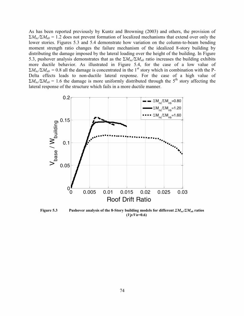
74

As has been reported previously by Kuntz and Browning (2003) and others, the provision of

ΣMnc/ΣMnb = 1.2 does not prevent formation of localized mechanisms that extend over only the

lower stories. Figures 5.3 and 5.4 demonstrate how variation on the column-to-beam bending

moment strength ratio changes the failure mechanism of the idealized 8-story building by

distributing the damage imposed by the lateral loading over the height of the building. In Figure

5.3, pushover analysis demonstrates that as the ΣΜnc/ΣΜnb ratio increases the building exhibits

more ductile behavior. As illustrated in Figure 5.4, for the case of a low value of

ΣΜnc/ΣΜnb = 0.8 all the damage is concentrated in the 1st story which in combination with the P-

Delta effects leads to non-ductile lateral response. For the case of a high value of

ΣΜnc/ΣΜnb = 1.6 the damage is more uniformly distributed through the 5th

story affecting the

lateral response of the structure which fails in a more ductile manner.

Figure 5.3 Pushover analysis of the 8-Story building models for different ΣΜnc/ΣΜnb ratios

(Vp/Vn=0.6)

0 0.005 0.01 0.015 0.02 0.025 0.030

0.05

0.1

0.15

0.2

Roof Drift Ratio

Vb

ase /

Wb

uild

ing

M

nc/M

nb=0.80

Mnc

/Mnb

=1.20

Mnc

/Mnb

=1.60

75

Figure 5.4 Failure mechanisms of the 8-Story building models for different ΣΜnc/ΣΜnb

ratios (Vp/Vn=0.6): (a) ΣΜnc/ΣΜnb=0.80 , (b) ΣΜnc/ΣΜnb=1.20 , and

(c) ΣΜnc/ΣΜnb=1.60

5.2 ASSESSMENT OF SEISMIC BEHAVIOR

Seismic behavior of the studied building models was assessed using the incremental dynamic

analysis (IDA) method. According to this method, an analytical model of a building was

subjected to numerous dynamic analyses under multiple ground motions scaled gradually to

increasing acceleration amplitude. Collapse was defined for the smallest input motion required to

(a)

(b)

(c)

76

achieve either one of the following two limit states: 1) Maximum story drift ratio exceeding 10%

of story-height, or 2) Shear or axial failure in more than 50% of the columns in any story.

More details regarding the IDA procedure followed in this study can be found in Chapter 4.

Figure 5.5 shows a typical output from an IDA of a single building. Each line in the figure

represents the response of the building to a single ground motion record scaled to increasing

intensity. Note that the curves begin to flatten out at maximum story drift ratio of approximately

0.05, suggesting that the structure becomes unstable at around this story drift ratio. The latter

value of story drift resulting in “dynamic” instability of the building is consistent with the results

obtained from pushover analysis (Figure 5.4-b ) where for story drift value of the 1st story

slightly less than 0.05, the pushover curve starts having negative stiffness slope indicating

“static” instability.

Figure 5.5 Incremental Dynamic Analysis (IDA) curves for the 8-story “modern code design”

building model (Vp/Vn=0.6, ΣΜnc/ΣΜnb=1.2)

The collapse risk of each building model was obtained from statistics on the IDA results. In this

study, collapse performance was evaluated using the probability of collapse as a function of the

ground motion intensity level, defined in terms of Sa(T1). The collapse probabilities in terms of

Sa(T1) were assumed to be log-normally distributed. Figure 5.6 shows the collapse fragility

relations. The interested reader can find a more detailed description of the fragility curve

development procedure in Chapter 4.

77

Figure 5.6 Collapse fragility functions of the “modern code design” building models

(Vp/Vn=0.6, ΣΜnc/ΣΜnb=1.2)

The variation of structural parameters (beam moment strength and column transverse

reinforcement) could lead to changes in the overall building strength. To avoid comparison bias

that could occur due to differences in building strength, the results of the study were normalized

with respect to the maximum base shear capacity of the frame Vmax. The value of Vmax was

calculated from non-linear static analysis with inverted triangular load pattern. The normalized

strength parameter Re was defined as:

max

1 )/()(

V

gWTSR

buildinga

e

(Eq. 5.1)

Note that Re represents approximately the ratio of elastic demand to actual strength. It is not the

same as the response modification coefficient R of ASCE 7-10, which is the ratio of the elastic

demand for the design earthquake level to the required design strength.

Calculation of the Re normalization factor requires the creation of a non-linear building model

which could be a cumbersome procedure. Alternatively a simpler normalization factor could be

used. The second normalization factor M uses an estimate of the maximum base shear capacity

of the building Vmax,estimated. The latter procedure requires only hand-calculations and it was

developed by Mehrain (ATC-78, 2013). The procedure used to compute the Vmax,estimated is

78

described in Appendix D. It should be noted that the described procedure to estimate the base

shear capacity of existing buildings includes numerous assumptions and, thus, it is just an

approximation that could be used as an alternative to sophisticated non-linear analysis for rapid

seismic risk evaluation. For clarity when this normalization method is used the normalized

parameter would be referred to as M, where:

estimated

buildinga

V

gWTSM

max,

1 )/()( (Eq. 5.2)

The normalization factor M is identical to the Re factor except for the calculation of the base

shear capacity that is computed as explained in Appendix D.

5.3 USING COLLAPSE INDICATORS TO PERFORM EARTHQUAKE RISK

ASSESSEMENT FOR EXISTING BUILDINGS

For buildings assigned to the highest Seismic Risk categories and having moment frames as the

seismic force-resisting system, ACI 318-11 requires that the moment frames be proportioned and

detailed as special moment frames. For such frames, ACI 318-11 requires that the sum of column

nominal moment strengths be at least 1.2 times the sum of beam nominal moment strengths at

every beam-column joint. (Some localized exceptions to this requirement can be permitted.) This

requirement is commonly referred to as the “strong-column, weak-beam” requirement. Its

purpose is to promote beam yielding rather than column yielding, thereby spreading flexural

yielding over multiple stories as the building responds to strong earthquake shaking. In buildings

with relatively weak columns, column hinging may lead to deformations concentrated in one

story, resulting in a so called weak-story mechanism. Older concrete buildings commonly do not

satisfy the strong-column, weak-beam requirement, making them more vulnerable to damage and

collapse because of the development of a weak story.

To study the effect of column-to-beam strength ratio on the collapse risk of buildings with

otherwise good details, the beam moment strengths were scaled to achieve column-to-beam

moment strength ratios ΣMnc/ΣMnb varying from 0.6 to 1.8. Transverse reinforcement was

sufficient to result in Vp/Vn = 0.6, such that shear failures were prevented in the study. Figure 5.7

presents partial results from the analyses, in this case plotting probability of collapse as a

function of ΣMnc/ΣMnb for Re = 3. A notable observation is that there is rapid increase in collapse

probability for values of ΣMnc/ΣMnb less than approximately 1.2, the minimum value permitted

by ACI 318-11 for special moment frames.

79

Figure 5.7 Comparison of collapse performance of the studied building models for Re=3 and

Vp/Vn=0.6

Figures 5.8 (a)-(c) depict the effect of ΣΜnc/ΣΜnb for different values of the parameter Re for the

three building frames. Note that in this figure, all the buildings have closely spaced transverse

reinforcement resulting in ductile flexural response without possibility of shear failure. From the

figure, several observations can be made. In general, collapse probability increases as Re

increases. For values of ΣΜnc/ΣΜnb = 1.2 and Re = 3, probability of collapse is approximately

10% for the four-story frame, increasing to approximately 20% for the 12-story frame. Thus, to

achieve the same probability of collapse, a larger value of ΣΜnc/ΣΜnb is required for taller

buildings than for shorter buildings.

0.0

0.1

0.2

0.3

0.4

0.5

0.6

0.7

0.8

0.9

1.0

0.6 0.8 1.0 1.2 1.4 1.6 1.8

Probability of Collapse

ΣΜnc / ΣΜnb

4-Story

8-Story

12-Story

80

Figure 5.8 Collapse Performance of (a) 4-Story (b) 8-Story (c) 12-Story building models with

Vp/Vn=0.6

Older-type concrete buildings commonly do not have closely spaced transverse reinforcement,

making them more susceptible to shear and axial failures. To study this effect, the spacing of

column transverse reinforcement was varied in each of the building models to achieve values of

Vp/Vn ranging from 0.6 to 1.2. For each value of Vp/Vn, ratios of column-to-beam moment

strengths ΣΜnc/ΣΜnb were varied from 0.6 to 1.8, creating a full matrix of results for the range of

Vp/Vn and ΣΜnc/ΣΜnb. For frames having Vp/Vn > 0.7, shear and axial failure was considered a

possibility. Therefore, for these frames, the analytical model was modified to enable simulation

of shear and axial failures.

Incremental dynamic analyses were conducted for each combination of the study variables.

Figure 5.9 presents collapse fragility curves evaluated from the IDA results. The figure conveys

information that can be interpreted in different ways. For example, for a given value of Re, the

collapse fragility is much higher for the frames with shear-critical columns than for frames with

flexure-controlled columns. Alternatively, for a building with shear-critical columns to have the

81

same collapse fragility as a frame with flexure-controlled columns, it must have higher base-

shear strength (that is, smaller Re).

Figure 5.9 Comparison of the fragility curves of the 8-Story Building having ΣΜnc/ΣΜnb=1.2

Figure 5.10 compares the effect of Vp/Vn for the 4, 8, and 12-story frames, in each case for

ΣΜnc/ΣΜnb = 1.2 and Re = 3. For each configuration, the collapse probability increases as the

transverse reinforcement spacing increases (that is, Vp/Vn increases). Also, for a given value of

Vp/Vn, a taller building is always more vulnerable than a shorter one. This is because shear failure

generally is restricted to a single story, such that most of the building lateral drift concentrates in

that story. In a tall building, a single-story failure represents a more severe localization and

therefore higher demand than occurs in an otherwise identical shorter building. P-delta effects

also are greater for a taller building, exacerbating strength loss and thereby accelerating failure.

0 2 4 6 80

0.2

0.4

0.6

0.8

1

Re

P[C

olla

pse]

Vp/V

n=0.6

Vp/V

n=1.0

VpV

n=0.8

Vp/V

n=1.2

82

Figure 5.10 Comparison of the collapse performance of the three Idealized Buildings for

ΣΜnc/ΣΜnb=1.2 and Re=3

Figure 5.11-5.13 present collapse probability results for the complete matrix of Vp/Vn and

ΣΜnc/ΣΜnb values that were investigated for the 4,8 and 12-story buildings. Collapse

probabilities increase with increasing Re, increasing Vp/Vn, and decreasing ΣΜnc/ΣΜnb. The

combination of low strength, high Vp/Vn, and low ΣΜnc/ΣΜnb is especially critical.

0.0

0.1

0.2

0.3

0.4

0.5

0.6

0.7

0.8

0.9

1.0

0.6 0.8 1.0 1.2


Vp/ Vn

4-Story

8-Story

12-Story

83

Figure 5.11 Comparison of the collapse performance of the 4-Story Building for

(a) Vp/Vn=0.6 , (b) Vp/Vn=0.8, (c) Vp/Vn=1.0 and (d) Vp/Vn=1.2

84



85



Figure 5.14 presents collapse probability results for the complete matrix of Vp/Vn and ΣΜ /ΣΜ

values for 4, 8, and 12-story frames. As previously noted, collapse probabilities increase with

increasing Vp/Vn, and decreasing ΣΜnc/ΣΜnb. The combination of low strength, high Vp/Vn, and

low ΣΜnc/ΣΜnb is especially critical, and more-so for taller frames than for shorter frames. For

the flexure-controlled frames (Figure 5.12a), collapse probabilities increase significantly for

ΣΜnc/ΣΜnb less than approximately 1.2 (the required value in ACI 318-11 for special moment

frames). For frames with shear-critical columns (Figure 5.12 b, c, and d), the critical value of

ΣΜnc/ΣΜnb appears to shift to higher values. A list of the probability of collapse values for all the

considered cases in a matrix format can be found in Appendix E.

86

Figure 5.14 Comparison of the collapse performance of the three Idealized Buildings with

Re=3 for (a) Vp/Vn=0.6 , (b) Vp/Vn=0.8 , (c) Vp/Vn=1.0 and (d) Vp/Vn=1.2

87

5.4 EARTHQUAKE RISK ASSESSEMENT FOR BUILDINGS WITH NON-

UNIFORM STRUCTURAL PARAMETERS

The results presented in the previous sections of this chapter correspond to the case of idealized

buildings that possess uniform structural parameters for all the structural components. Although

this presents a convenient simplification, since collapse potential is directly linked to a change in

the value of one structural parameter, this is hardly the case for any existing building. In reality

most of the buildings consist of components with varying structural parameter (collapse

indicator) values, even within the same story.

In the current section the effect of varying ΣMnc/ΣΜnb values within a story of a building was

explored. In the original idealized 8-story buildings, joints A,B,C,D,E, and F illustrated in Figure

5.15 possess uniform ΣMnc/ΣΜnb values for all the stories except the roof.

Figure 5.15 Illustration of joins A,B,C,D,E, and F of the 8-story idealized building

To study the effect of ΣMnc/ΣΜnb parameter variation, the beam moment strengths were modified

such that different combinations of ΣMnc/ΣΜnb values for each joint in the same story are

obtained. The effect was studied based on the 8-story idealized building.

The considered combinations are presented in Table 5.1. The modification of beam strength

values was performed such that all the stories possess exactly the same joint ΣMnc/ΣΜnb

combination values.

88

Table 5.1 Combination of non-uniform join ΣΜnc/ΣΜnb values

Joint ΣΜnc/ΣΜnb values

Non-Uniform ΣΜnc/ΣΜnb Combination

Story Average4 <ΣΜnc/ΣΜnb>

A B C D E F

1 0.8 1.0 0.8 0.6 0.6 0.8 1.0

2 1.0 1.2 1.0 0.8 0.8 1.0 1.2

3 1.0 1.4 1.0 0.6 0.6 1.0 1.4

4 1.2 1.4 1.2 1.0 1.0 1.2 1.4

5 1.2 1.6 1.2 0.8 0.8 1.2 1.6

6 1.2 1.8 1.2 0.6 0.6 1.2 1.8

7 1.4 1.6 1.4 1.2 1.2 1.4 1.6

8 1.4 1.8 1.4 1.0 1.0 1.4 1.8

9 1.6 1.8 1.6 1.4 1.4 1.6 1.8

The collapse performance of each model with certain ΣMnc/ΣΜnb joint combinations was

reported. Consequently the collapse performance of each considered model with non-uniform

ΣMnc/ΣΜnb joint values was compared with the performance of an idealized frame with uniform

ΣMnc/ΣΜnb joint values.

The collapse performance of the studied models with uniform (solid lines) and non-uniform

(dashed lines) ΣMnc/ΣΜnb joint values is presented in Figure 5.16.

4 Story average is calculated as follows:

6

)/(

/

F

Ak

knbnc

nbnc

89

Figure 5.16 Comparison of the collapse performance of the idealized 8-story building with: a)

uniform ΣΜnc/ΣΜnb values, and b) non-uniform ΣΜnc/ΣΜnb values

The results suggest that buildings with non-uniform ΣΜnc/ΣΜnb joint values, and with story

average <ΣΜnc/ΣΜnb>=B have similar collapse performance as the idealized buildings that

possess uniform ΣΜnc/ΣΜnb=B joint values. Therefore, story average <ΣΜnc/ΣΜnb> seems to be

a relatively good indicator of the collapse performance of buildings that possess non-uniform

joint ΣΜnc/ΣΜnb values.

For the purposes of the ATC-78 project (ATC-78, 2013) Dr. Liel and her colleagues performed a

similar study to explore the effect of varying Vp/Vn parameter for columns within the same story.

The study was performed using a one story frame with multiple columns. Each column in that

frame was assigned random transverse reinforcement ratio values such that it would correspond

to a different Vp/Vn ratio values. Random realizations of each column transverse reinforcement

characteristics were generated using Monte Carlo simulations. In the simulations the collapse

performance of each one-story frame consisting of columns with different Vp/Vn ratios was

evaluated using IDA. The results of Dr. Liel’s study demonstrated that story average of the

column Vp/Vn ratio is a relatively good indicator of the response of frames.

0.0

0.1

0.2

0.3

0.4

0.5

0.6

0.7

0.8

0.9

1.0

2 3 4 5 6


Re

Mc/Mb=0.8 (uniform)

Mc/Mb=1.0 (uniform)

Mc/Mb=1.2 (uniform)

Mc/Mb=1.4 (uniform)

Mc/Mb=1.6 (uniform)

Combination 1

Combination 2

Combination 3

Combination 4

Combination 5

Combination 6

Combination 7

Combination 8

Combination 9

90

5.5 LIMITATIONS OF THE STRENGTH-BASED APPROACH IN COLLAPSE

EVALUATION

In the current chapter a methodology to evaluate the building collapse potential using simple

engineering parameters was presented. The results of this study are limited to buildings

possessing concrete moment frames to resist the earthquake loading. Buildings suffering from

structural deficiencies other than those addressed in the current study (weak column

mechanisms, shear critical columns) cannot be evaluated with the collapse evaluation approach

presented in this Chapter. Although strength-based normalization parameters (Re and M) were

utilized to avoid comparison bias of buildings with different building strengths, the results of the

current study should be applied with caution for buildings having very different strength and

geometrical properties compared to the considered frames. Very tall buildings (taller than 12

stories) that are significantly influenced by higher mode effects or buildings suffering from

severe vertical and plan irregularities were not considered in the current study.

91

6 A Displacement-Based Methodology to Evaluate

the Collapse Potential of Older-Type Concrete

Frame Buildings

In Chapter 5, a method to estimate the collapse potential of older-type concrete buildings was

presented. Due to the inability to evaluate all possible building variations, the normalization

factors Re and M were utilized. Both normalization factors were defined such that seismic

demand was normalized with respect to base shear strength. This normalization was employed

such that it would reduce a potential comparison bias between buildings with similar geometry

but different building strength. According to the methodology presented in Chapter 5 the

probability of collapse of a certain building, possessing certain collapse indicator parameters is

estimated based on its base shear strength and the earthquake intensity. In other words for the

same building geometry, structural parameters (ΣΜnc/ ΣΜnb and Vp/Vn) and earthquake intensity,

higher strength would lead to lower Re (and M) and thus to lower probability of collapse.

Although the approach presented in the previous Chapter seems to provide rational results, it

suffers from one main disadvantage. According to the IDA procedure used to evaluate building

collapse potential, the performance of a building is judged according to member deformations or

story displacements. Thereby it is more intuitive to develop a methodology in which, for certain

earthquake intensity, a parameter based on displacement rather than based on strength (like Re or

M) would influence the building collapse potential.

In the current Chapter an alternative approach using a displacement based method to evaluate

building collapse is proposed. Initially, a procedure to estimate story drift ratio demand is

presented given the dynamic properties of the considered building and the earthquake intensity

level. The IDA results of the three idealized buildings presented in Chapter 4 are used to

calibrate the parameters employed for calculation of story drift ratio demands. Consequently the

estimated story drift ratio demand is shown that can be related to column drift capacity to

estimate column failure potential. Finally, a simplified method that links column failure potential

with building collapse performance, using only hand-calculations, is presented.

6.1 DETERMINATION OF STORY DRIFT RATIO DEMAND

A basic issue related with the collapse performance of structural systems is the determination of

story drift ratio demand. In the current section the idealized buildings developed in Chapter 4

will be used to get insight on how story drift ratio demand can be estimated for variations of the

idealized buildings considered in the current study using a simplified approach.

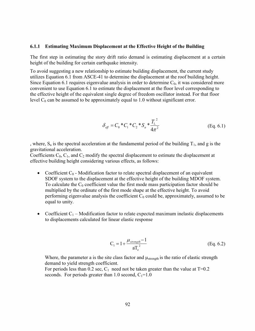
92

6.1.1 Estimating Maximum Displacement at the Effective Height of the Building

The first step in estimating the story drift ratio demand is estimating displacement at a certain

height of the building for certain earthquake intensity.

To avoid suggesting a new relationship to estimate building displacement, the current study

utilizes Equation 6.1 from ASCE-41 to determine the displacement at the roof building height.

Since Equation 6.1 requires eigenvalue analysis in order to determine C0, it was considered more

convenient to use Equation 6.1 to estimate the displacement at the floor level corresponding to

the effective height of the equivalent single degree of freedom oscillator instead. For that floor

level C0 can be assumed to be approximately equal to 1.0 without significant error.

2

2

.1210

4****

TSCCC aeff (Eq. 6.1)

, where, Sa is the spectral acceleration at the fundamental period of the building T1, and g is the

gravitational acceleration.

Coefficients C0, C1, and C2 modify the spectral displacement to estimate the displacement at

effective building height considering various effects, as follows:

Coefficient C0 - Modification factor to relate spectral displacement of an equivalent

SDOF system to the displacement at the effective height of the building MDOF system.

To calculate the C0 coefficient value the first mode mass participation factor should be

multiplied by the ordinate of the first mode shape at the effective height. To avoid

performing eigenvalue analysis the coefficient C0 could be, approximately, assumed to be

equal to unity.

Coefficient C1 – Modification factor to relate expected maximum inelastic displacements

to displacements calculated for linear elastic response

2

e

1aT

11C

strength (Eq. 6.2)

Where, the parameter a is the site class factor and μstrength is the ratio of elastic strength

demand to yield strength coefficient.

For periods less than 0.2 sec, C1 need not be taken greater than the value at T=0.2

seconds. For periods greater than 1.0 second, C1=1.0

93

Coefficient C2 – modification factor to represent the effect of pinched hysteresis shape,

cyclic stiffness degradation, and strength deterioration on maximum displacement

response

2

G.F.

2T

1

800

11C

strength (Eq. 6.3)

For periods greater than 0.7 sec, C2=1.0

(The interested reader can find further information regarding the procedure followed in section

6.3.2 in Chapter 7 of ASCE-41)

The coefficients C0 , C1 and C2 employed in Equation 6.1 for the idealized buildings considered

in the current study are presented in the Table 6.1 cited below:

Table 6.1 Coefficients of the studied buildings utilized in equation 6.1

Building

4-Story 8-Story 12-Story

T1 (sec) 1.14 1.62 1.95

C0 1.05 1.09 1.08

C1 1.00 1.00 1.00

C2 1.00 1.00 1.00

6.1.1.1 Comparison of Estimated Floor Displacements and Non-Linear Response History

Analysis

Equation 6.1 provides an estimate of maximum displacement at the effective modal height floor

level for a given spectral acceleration value. In order to verify the validity of the provided

equation, statistical processing of the results obtained through IDA was performed for variations

of the idealized buildings.

The studied cases included buildings with components whose failure was flexural, shear or

axially dominated.

The results of the comparison are presented in the tables below:

94

Table 6.2 Mean ratio of (maximum displacement at effective modal height floor level of non-linear

analysis) / (estimated displacement at effective modal height floor level of equation 6.1) for

different Vp/Vn and ΣMnc/ΣMnb ratios of the 4-Story Idealized Building

Vp/Vn

ΣΜnc/ΣΜnb 0.6 0.8 1.0 1.2

0.6 0.88 0.80 0.82 0.91

0.8 0.88 0.80 0.82 0.91

1.0 0.87 0.81 0.81 0.90

1.2 0.92 0.82 0.83 0.85

1.4 0.99 0.85 0.85 0.84

1.6 1.12 0.91 0.86 0.85

1.8 1.17 0.94 0.91 0.87




Vp/Vn

ΣΜnc/ΣΜnb 0.6 0.8 1.0 1.2

0.6 0.84 0.84 0.85 0.94

0.8 0.84 0.83 0.85 0.92

1.0 0.84 0.83 0.84 0.91

1.2 0.87 0.82 0.81 0.83

1.4 1.01 0.90 0.87 0.86

1.6 1.12 0.97 0.93 0.91

1.8 1.23 1.01 0.98 0.96

95




Vp/Vn

ΣΜnc/ΣΜnb 0.6 0.8 1.0 1.2

0.6 0.95 0.96 0.97 0.99

0.8 0.94 0.96 0.97 1.00

1.0 0.94 0.94 0.96 0.96

1.2 0.99 0.96 0.93 0.90

1.4 1.25 1.10 1.02 0.96

1.6 1.42 1.18 1.10 1.05

1.8 1.46 1.24 1.16 1.12

Tables 6.2-6.4 demonstrate that for most of the cases equation 6.1 provides a conservative

estimate of the maximum displacement at the effective modal height. The accuracy of the

displacement estimation at the effective modal height floor level improves as the ratio of column

to beam moment strength increases.

Since the modal period of the studied buildings is relatively high, the equal displacement rule

(Chopra 2011) should hold approximately. In Equation 6.1 factors C1 and C2 are assumed to be

equal to unity, in accordance with the fact that maximum floor displacements are expected to be

overall independent of the base shear strength of the building.

In order to verify the assumption that the estimated displacement provided by Equation 6.1 is not

influenced by the building strength, the displacements at the effective building height obtained

from IDA for different values of Re= Sa*Wbuidling / Vmax were compared with those estimated by

Equation 6.1. In Figure 6.1 the aforementioned comparison is performed for the 8-story idealized

building. In Figure 6.1 each point corresponds to a scaled ground motion non-linear analysis

result which was used for IDA.

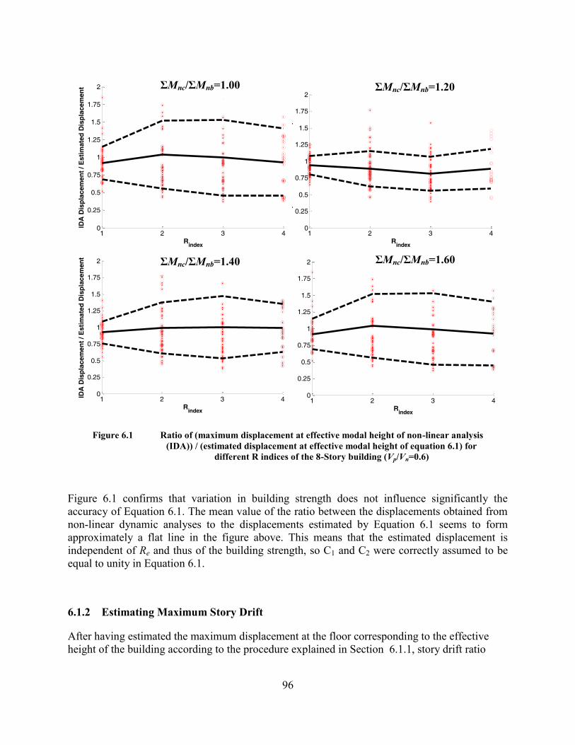
96

Figure 6.1 Ratio of (maximum displacement at effective modal height of non-linear analysis

(IDA)) / (estimated displacement at effective modal height of equation 6.1) for

different R indices of the 8-Story building (Vp/Vn=0.6)

Figure 6.1 confirms that variation in building strength does not influence significantly the

accuracy of Equation 6.1. The mean value of the ratio between the displacements obtained from

non-linear dynamic analyses to the displacements estimated by Equation 6.1 seems to form

approximately a flat line in the figure above. This means that the estimated displacement is

independent of Re and thus of the building strength, so C1 and C2 were correctly assumed to be

equal to unity in Equation 6.1.

6.1.2 Estimating Maximum Story Drift

After having estimated the maximum displacement at the floor corresponding to the effective

height of the building according to the procedure explained in Section 6.1.1, story drift ratio

1 2 3 40

0.25

0.5

0.75

1

1.25

1.5

1.75

2

Rindex

ID

A D

isp

lacem

en

t / E

sti

mate

d D

isp

lacem

en

t

1 2 3 40

0.25

0.5

0.75

1

1.25

1.5

1.75

2

Rindex

ID

A D

isp

lac

em

en

t / E

sti

ma

ted

Dis

pla

ce

me

nt

1 2 3 40

0.25

0.5

0.75

1

1.25

1.5

1.75

2

Rindex

ID

A D

isp

lac

em

en

t / E

sti

ma

ted

Dis

pla

ce

me

nt

1 2 3 40

0.25

0.5

0.75

1

1.25

1.5

1.75

2

Rindex

ID

A D

isp

lac

em

en

t / E

sti

ma

ted

Dis

pla

ce

me

nt

ΣΜnc/ΣΜnb=1.20

ΣΜnc/ΣΜnb=1.40 ΣΜnc/ΣΜnb=1.60

ΣΜnc/ΣΜnb=1.00

97

demand needs to be estimated for each story. Figure 6.2 illustrates the general concept. That

figure demonstrates the drift profile of two extreme cases:

a) Uniform story drift pattern which would ideally apply for a building with very high column-

to-beam moment strength ratio, and

b) Weak story drift pattern which would ideally apply for the case of building in which the first

story has very low column-to-beam moment strength ratios.

(It is recognized that both these patterns correspond to extreme cases that would rarely appear in

an existing building but are provided for the purpose of illustrating the presented concept.)

Figure 6.2 Two idealized story drift patterns for an example building frame

From the example of the two idealized story drift patterns presented above, it becomes obvious

that the story drift profile depends largely on the column-to-beam bending moment ratio. In the

current study the variable “alpha” (α), is used to estimate the maximum story drift demand as

shown in Equation 6.4.

eff

eff

x

x

xDx

ha

h

* (Eq. 6.4)

where, δx is the story drift demand, hx is the story height, αx is the coefficient for story x used to

approximate the expected story drift pattern, δeff is the estimated displacement at the effective

height according to Equation 6.1, heff is the effective building height (it can be assumed that

heff ≈ 0.7*hbuilding,, where hbuidling is the total building height). In Equation 6.4, αx is used as an

amplification factor of the estimated average drift ratio (δeff/heff) at the effective height of the

building to the maximum story drift ratio demand ( Dx =δx/hx) at story x. For the idealized

uniform story drift pattern αx=1.0 for all stories while for the idealized weak story drift pattern

α1=heff/h1 and αx≠1=0.0.

δeff

δ1

δi level i

heff hi

δi

δeff

(a) Building Elevation

(c) Idealized uniform drift

pattern

(b) Equivalent SDOF system

(d) Idealized weak story drift

pattern

98

6.1.2.1 Determination of Coefficient α

The coefficient α, was calibrated to match approximately the dynamic response of the idealized

buildings considered in this study. It should be noted that these buildings were designed such that

they possess uniform structural parameters Vp/Vn and ΣΜnc/ΣMnb. Using results obtained from

numerous non-linear dynamic analysis performed as part of the IDA procedure discussed in

Chapter 4, the values of coefficient α were recorded for ground motion scaling factors slightly

less than the factor required to achieve collapse. Statistical regression was performed between

the estimated average drift ratio at the effective building height δeff/heff (predictor) and the

maximum story drift ratio demand δx/hx (response variable). The procedure was repeated for

each story according to Equation 6.4. The coefficient αx was chosen such that the sum of the

square errors of Equation 6.4 to the data is minimized. Further information regarding the

statistical procedure performed to estimate coefficient αx is provided in Appendix G.

Buildings with Uniform DCRs

As discussed in Chapter 4 the idealized buildings developed for the purpose of this study have

approximately uniform Demand over Capacity Ratio (DCR) (see Appendix D).

Figures 6.3-6.5 show the least square estimates of the coefficient αx values for different

variations of the idealized buildings which are representative of buildings that tend to have

uniform strength characteristics and do not possess any significant strength deficiencies along the

height.

99


buildings

0 0.5 1 1.5 21

2

3

4

x

Sto

ry

Vp/V

n=0.8

Mnc

/Mnb

=0.60

Mnc

/Mnb

=0.80

Mnc

/Mnb

=1.00

Mnc

/Mnb

=1.20

Mnc

/Mnb

=1.40

Mnc

/Mnb

=1.60

Mnc

/Mnb

=1.80

0 0.5 1 1.5 21

2

3

4

x

Sto

ry

Vp/V

n=1.0

0 0.5 1 1.5 21

2

3

4

x

Sto

ry

Vp/V

n=1.2

100

Figure 6.3-b Alpha coefficient value at the 1st story for different variations of the 4-story

idealized building

0.6 0.8 1 1.2 1.4 1.6 1.80

0.5

1

1.5

2

Mnc

/Mnb

1

Vp/V

n=0.8

Vp/V

n=1.0

Vp/V

n=1.2

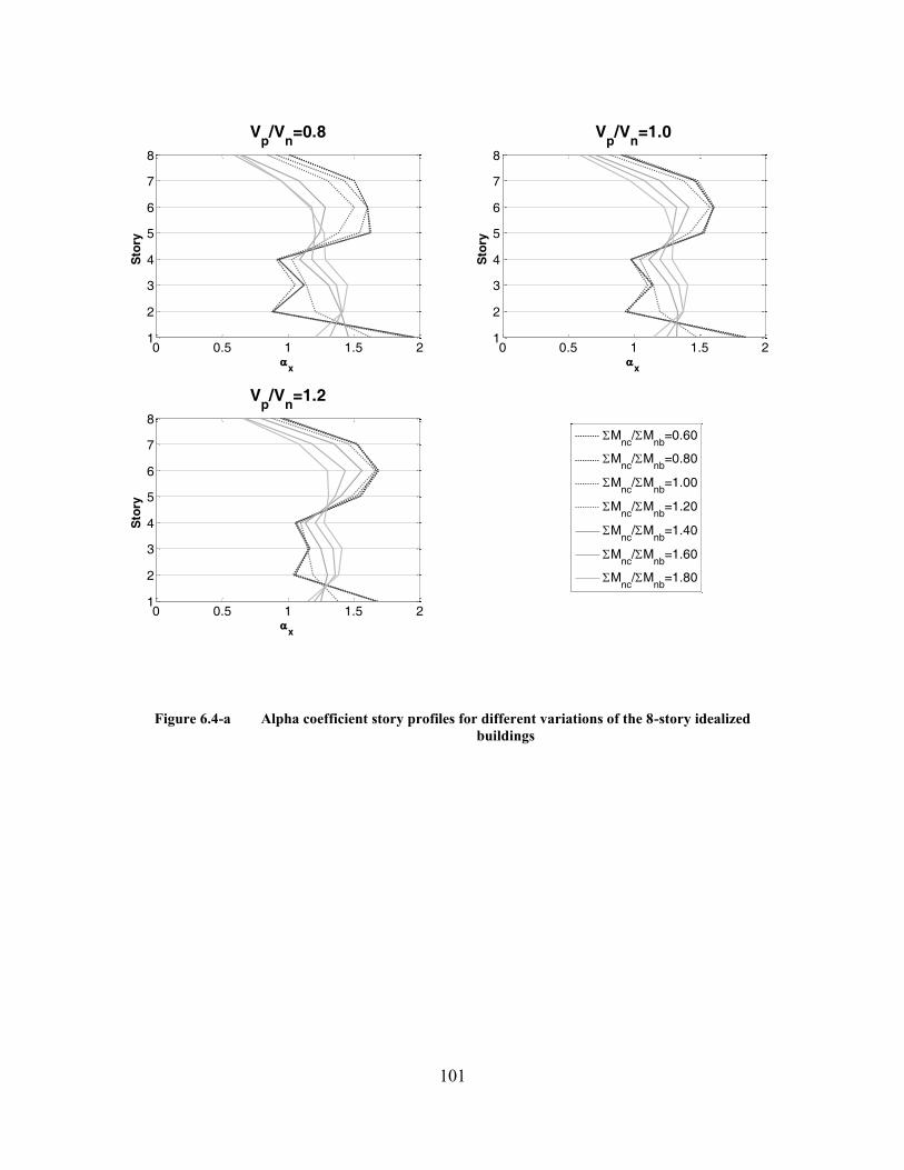
101


buildings

0 0.5 1 1.5 21

2

3

4

5

6

7

8

x

Sto

ry

Vp/V

n=0.8

Mnc

/Mnb

=0.60

Mnc

/Mnb

=0.80

Mnc

/Mnb

=1.00

Mnc

/Mnb

=1.20

Mnc

/Mnb

=1.40

Mnc

/Mnb

=1.60

Mnc

/Mnb

=1.80

0 0.5 1 1.5 21

2

3

4

5

6

7

8

x

Sto

ry

Vp/V

n=1.0

0 0.5 1 1.5 21

2

3

4

5

6

7

8

x

Sto

ry

Vp/V

n=1.2

102

Figure 6.4-b Alpha factor coefficient at the 1st story for different variations of the 8-story

idealized building

0.6 0.8 1 1.2 1.4 1.6 1.80

0.5

1

1.5

2

Mnc

/Mnb

1

Vp/V

n=0.8

Vp/V

n=1.0

Vp/V

n=1.2

103


buildings

0 0.5 1 1.5 21

2

3

4

5

6

7

8

9

10

11

12

x

Sto

ry

Vp/V

n=0.8

Mnc

/Mnb

=0.60

Mnc

/Mnb

=0.80

Mnc

/Mnb

=1.00

Mnc

/Mnb

=1.20

Mnc

/Mnb

=1.40

Mnc

/Mnb

=1.60

Mnc

/Mnb

=1.80

0 0.5 1 1.5 21

2

3

4

5

6

7

8

9

10

11

12

x

Sto

ry

Vp/V

n=1.0

0 0.5 1 1.5 21

2

3

4

5

6

7

8

9

10

11

12

x

Sto

ry

Vp/V

n=1.2

104

Figure 6.5-b Alpha factor coefficient at the 1st story for different variations of the 12-story

idealized building

Figures 6.3 to 6.5 demonstrate that αx is mainly influenced by the ΣΜnc/ΣMnb ratio, and is less

dependent on the Vp/Vn ratio.

A detailed presentation of the αx values obtained for variations of the idealized buildings is

presented in Appendix G.

Buildings with Non-Uniform DCRs

As observed in Figures 6.3 to 6.5 the values of coefficient αx vary along the height of the

building. Intuition suggests that αx should have higher values at the story x of the building that is

the “weakest” (the term weak here corresponds to shear strength capacity of the structural

components and is not related with their deformation characteristics). One way to identify the

weakest story is by looking at the DCRs of the stories for the considered building. According to

this procedure the story that has significantly higher DCR than the rest of the stories can be

characterized as the weakest.

In this section, the 8-story building was selected to demonstrate how possessing a weak story at

the mid-height could alter the story drift profiles.

Figure 6.6 illustrates the alpha story profile values for variations of the 8-story building with a

critical story at the mid-height (critical 4th

story).

The critical 4th

story building corresponds to a variation of the originally developed idealized 8-

story building. For the latter, the columns at the 4th

story of the idealized 8-story building were

modified such that DCR4th=1.30*DCR1st. (critical 4th

story). This variation of the 8-story building

0.6 0.8 1 1.2 1.4 1.6 1.80

0.5

1

1.5

2

Mnc

/Mnb

1

Vp/V

n=0.8

Vp/V

n=1.0

Vp/V

n=1.2

105

is compared with the response of the originally developed idealized building which possesses

approximately uniform DCRs along the height.

Figure 6.6-a Comparison of the alpha coefficient story profiles for the 8-story with uniform

DCRs (idealized building) and with critical story at the mid-height (Vp/Vn=0.8 for

both cases) (for the critical 4th

story case DCR4th=1.30DCR1st)

0 0.5 1 1.5 21

2

3

4

5

6

7

8

x

Sto

ry

Idealized Building

Mnc

/Mnb

=0.80

Mnc

/Mnb

=1.20

Mnc

/Mnb

=1.60

0 0.5 1 1.5 21

2

3

4

5

6

7

8

x

Sto

ry

Critical 4th

Story

Mnc

/Mnb

=0.80

Mnc

/Mnb

=1.20

Mnc

/Mnb

=1.60

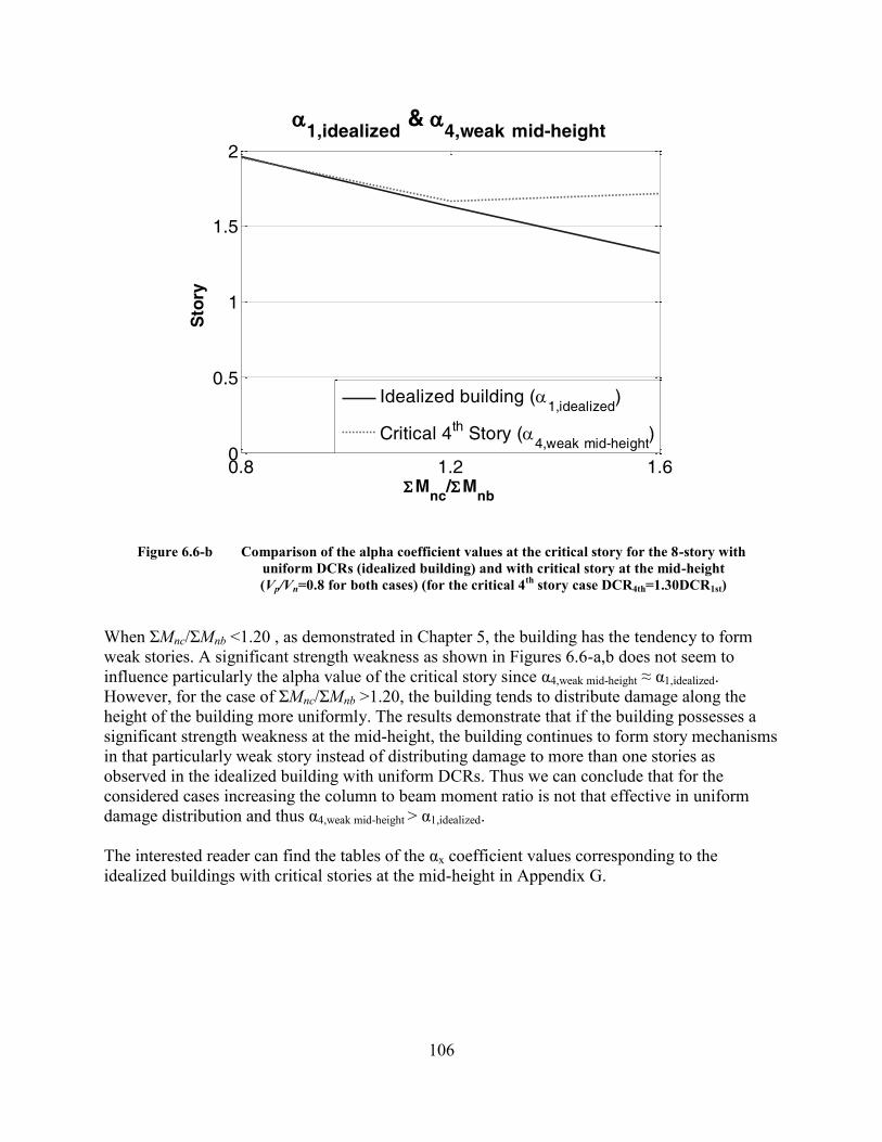
106

Figure 6.6-b Comparison of the alpha coefficient values at the critical story for the 8-story with

uniform DCRs (idealized building) and with critical story at the mid-height

(Vp/Vn=0.8 for both cases) (for the critical 4th

story case DCR4th=1.30DCR1st)

When ΣΜnc/ΣΜnb <1.20 , as demonstrated in Chapter 5, the building has the tendency to form

weak stories. A significant strength weakness as shown in Figures 6.6-a,b does not seem to

influence particularly the alpha value of the critical story since α4,weak mid-height ≈ α1,idealized.

However, for the case of ΣΜnc/ΣΜnb >1.20, the building tends to distribute damage along the

height of the building more uniformly. The results demonstrate that if the building possesses a

significant strength weakness at the mid-height, the building continues to form story mechanisms

in that particularly weak story instead of distributing damage to more than one stories as

observed in the idealized building with uniform DCRs. Thus we can conclude that for the

considered cases increasing the column to beam moment ratio is not that effective in uniform

damage distribution and thus α4,weak mid-height > α1,idealized.

The interested reader can find the tables of the αx coefficient values corresponding to the

idealized buildings with critical stories at the mid-height in Appendix G.

0.8 1.2 1.60

0.5

1

1.5

2

Mnc

/Mnb

Sto

ry

1,idealized

& 4,weak

mid-height

Idealized building (1,idealized

)

Critical 4th

Story (4,weak

mid-height

)

107

Buildings with column bars having inadequate lap splicing conditions

For the case of buildings having inadequate lap splice length for column longitudinal

reinforcement, with insufficient column confinement, as defined by ACI 318-11 (ACI, 2011), bar

slip and eventual failure of the lap splices might occur. Associated damage is likely to result in

rapid loss of moment resistance at the location of the lap splice.

To study the effects of this behavior on overall building response, a strength-degrading plastic

hinge was introduced at assumed locations of lap splices in the model buildings. The inadequate

lap splicing conditions were modeled according to the experimental results provided by Melek

and Wallace (2004). The backbone rotational behavior of the plastic hinges to model the

inadequate lap splicing conditions is shown in Figure 6.7.

Figure 6.7 Assumed zero-length plastic hinge rotational behavior for inadequate lap-splicing

conditions

Nonlinear dynamic analyses were conducted on model frames with flexure-critical columns

(Vp/Vn 0.8) including lap splices. Frames with different ΣΜnc/ΣΜnb ranging from 0.8 to 1.6 were

investigated. Figure 6.8 illustrates representative results for the case of lap splices introduced

into the base of the column members located in the 1st story of the 8-story frame.

The results demonstrate that, for the case of buildings with a tendency to form weak stories (that

is, ΣΜnc/ΣΜnb ≤ 1.20), the lap-splice has minimal effect, while the effect is slightly more

pronounced for cases where the building has a tendency to form a more uniform drift profile

(that is, ΣΜnc/ΣΜnb > 1.20). Apparently, the former case corresponds to a case for which a weak

story is already formed because of the weak columns, such that further reduction in strength due

to splice failure does not significantly exacerbate the story failure. For the latter case, the

presence of the lap splice results in reduced moment strength at one end of the column if the

column yields, which tends to produce a weak-story condition. However, because the columns

0

0.2

0.4

0.6

0.8

1

1.2

0 0.05 0.1

M/M

y

Plastic Rotation (rad)

108

are stronger than the beams, the extent of column yielding is reduced, such that the alpha factor

again is not much affected.

Due to the relatively small effect of lap splicing in the αx values of the considered cases, for the

purposes of the current study, the αx coefficient values can be approximately assumed to be the

same for both adequate and inadequate lap splicing conditions.

Figure 6.8-a Comparison of the alpha coefficient story profiles for different variation of the 8-

story idealized building with adequate and inadequate lap splicing conditions at

the base of the 1st story (Vp/Vn=0.8 for both cases)

0 0.5 1 1.5 21

2

3

4

5

6

7

8

x

Sto

ry

Adequate Lap Splice

Mnc

/Mnb

=0.60

Mnc

/Mnb

=0.80

Mnc

/Mnb

=1.00

Mnc

/Mnb

=1.20

Mnc

/Mnb

=1.40

Mnc

/Mnb

=1.60

Mnc

/Mnb

=1.80

0 0.5 1 1.5 21

2

3

4

5

6

7

8

x

Sto

ry

Inadequate Lap Splice

Mnc

/Mnb

=0.60

Mnc

/Mnb

=0.80

Mnc

/Mnb

=1.00

Mnc

/Mnb

=1.20

Mnc

/Mnb

=1.40

Mnc

/Mnb

=1.60

Mnc

/Mnb

=1.80

109

Figure 6.8-b Comparison of the alpha coefficient value at the critical 1st story for different

variations of the 8-story idealized building with adequate and inadequate lap

splicing conditions at the base of the 1st story (Vp/Vn=0.8 for both cases)

The suggestions regarding the lap-splicing conditions were based on limited studies performed

on the idealized buildings considered in the current study. Further study needs to be conducted in

the future in order to provide more general suggestions regarding the assessment of buildings

with such deficiencies.

The interested reader can find the results of the analyses performed to obtain the effect of

inadequate column bar lap splicing in Appendix G.

0.6 0.8 1 1.2 1.4 1.6 1.80

0.5

1

1.5

2

Mnc

/Mnb

1

Adequate Lap Splice

Inadequate Lap Splice

110

6.2 DETERMINATION OF COLUMN DRIFT CAPACITY

In the previous section a procedure to estimate the story drift ratio demand was presented. In the

current section it is attempted to define a similar procedure to estimate the column drift capacity.

Shear Critical Column Members

For shear critical columns possessing 0.7≤Vp/Vn≤1.2 column drift capacity can be determined

according to Equation 6.5 as suggested by Elwood (2002).

cgc

CxfA

P

f

v

'**)

40

1(

'*)500/1(''*403.0 (Eq. 6.5)

where ρ’’ is the column transverse reinforcement ratio, ν is the applied shear stress (provided in

psi units), f’c is the expected concrete stress (provided in psi units), P is the column axial load

(provided in lb units), Ag the column gross sectional area (provided in in2 units).

Columns having Inadequate Lap Splicing Conditions

Columns having longitudinal bars with inadequate lap splicing conditions are expected to start

degrading at or before they reach their shear yielding capacity (corresponding to flexural

yielding at the column ends). Thus, Equation 6.6 corresponds to a relatively conservative

estimate of their drift capacity. Further study is required to develop less conservative capacity

relationships.

01.0/**6

,

xeff

bottomy

CxhIE

M (Eq. 6.6)

where My,bottom corresponds to the yielding moment at the base of the column, E is the concrete

Young’s modulus, Ieff is the effective stiffness, and hx is story x height.

The column drift capacity that was assigned for such columns was approximated so that it

corresponds to total column rotation where the column has degraded to moment equal to 80% of

the maximum observed moment (80% of the yielding moment in that case). The relationship

providing the column drift capacity is given in Equation 6.6 and is computed such that it is

consistent with the modeling assumptions of inadequate lap splicing for longitudinal column

reinforcement followed in the current study.

111

6.3 A METHODOLOGY TO ESTIMATE THE COLUMN FAILURE POTENTIAL

In sections 6.2 and 6.3 procedures to estimate story drift demand and column drift capacity were

defined. Since the same quantity, drift, was used to describe both demand and capacity a direct

comparison between the two is possible. This comparison could provide an estimate of whether

an individual column member located in story x is likely to fail.

In the current section, a method to evaluate column failure potential is presented. The method is

based on the results presented above. Sections 6.1 and 6.2 are revisited and estimation of story

drift demand and column drift capacity is presented using a simplified approach that requires

only hand-calculations.

6.3.1 Estimating Column Drift Demand using only Hand Calculations

In similar fashion with Chapter 5, basic information that can be easily found after review of the

structural drawings or estimated using simple hand calculations are employed as the basic input

parameters to estimate column drift demand at story x.

The basic input parameters required correspond to the geometry of the structural system, member

dimensions, and reinforcement details.

The structural parameters that were linked with the collapse performance of the considered

buildings in this study were the following:

a) The column-to-beam bending moment strength ratio,

b) The shear demand over shear capacity ratio

c) Determination of potential column bar inadequate lap splice conditions

To apply the procedure described in Section 6.1, a certain earthquake intensity level needs to be

provided. The earthquake intensity is given as Spectral Acceleration Sa(T1) at the first

fundamental period of the building. To estimate the fundamental period of the building an

engineer has two options:

a) Perform eigenvalue analysis for the considered building

b) Apply Equation 6.7 to estimate T1. The latter equation was derived specifically for the

purposes of the current study based on statistical regression of concrete frame buildings.

The interested reader can find more details regarding the procedure followed to derive

Equation 6.7 in Appendix F.

69.039.0

.. )(**072.0,

W

VHT FG (Eq. 6.7)

where W is the weight of the building , V is the estimated base shear capacity (should be

estimated according to the procedure presented in Appendix E for Vmax,estimated) (V and W should

be provided in the same units), and H is the height of the building given in feet.

After all the structural parameters of the building have been calculated, the procedure presented

in Section 6.1 can be followed to estimate the average drift ratio δeff/heff .

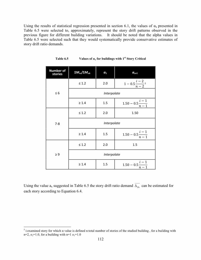
112

Using the results of statistical regression presented in section 6.1, the values of αx presented in

Table 6.5 were selected to, approximately, represent the story drift patterns observed in the

previous figure for different building variations. It should be noted that the alpha values in

Table 6.5 were selected such that they would systematically provide conservative estimates of

story drift ratio demands.

Table 6.5 Values of αx for buildings with 1st Story Critical

Number of stories ΣΜnc/ΣΜnb α1 αx≠1

≤ 6

≤ 1.2 2.0

5

Interpolate

≥ 1.4 1.5

7-8

≤ 1.2 2.0 1.50

Interpolate

≥ 1.4 1.5

≥ 9

≤ 1.2 2.0 1.5

Interpolate

≥ 1.4 1.5

Using the value ax suggested in Table 6.5 the story drift ratio demand Dx can be estimated for

each story according to Equation 6.4.

5 i:examined story for which α value is defined n:total number of stories of the studied building , for a building with

n=2, α2=1.0, for a building with n=1 α1=1.0

113

6.3.1.1 Uncertainty in Estimation of Column Drift Demand

As discussed in Section 6.1, statistical regression using the results from a number of non-linear

dynamic analyses was performed to estimate story drift ratio demands for the studied buildings.

For simplification purposes, αx values suggested in Table 6.5 are only a function of the column-

to-beam moment strength ratio. In reality the relation between the average drift and the story

drift demand is influenced by various factors not considered in the simple regression model

employed for the purposes of the current study. Among others, these factors include, earthquake

characteristics, building geometry, and building dynamic properties. The source of uncertainty

that is observed in the column drift demand is both epistemic (use of a simplified regression

formula not representing all the influential factors that determine the story drift patterns) and

aleatory (record-to-record variability).

The uncertainty in the estimation of story drift ratio demand ranges from 0.10 to 0.70 (see

Appendix G). On the basis of these data, the approximate values of standard deviation reported

in Table 6.6 are suggested for application in the suggested methodology.

Table 6.6 Uncertainty in predictions of drift demand

Number of stories σln,ΔD1 σln,ΔDx≠1

≤ 6 0.40 0.40

7-8 interpolate values

≥ 9 0.50 0.50

6.3.2 Estimating Column Drift Capacity

Information from the building drawings regarding the detailing characteristics of individual

column members could be utilized to estimate column drift capacity according to the procedure

described in Section 6.2. Two basic terms need to be estimated in order to evaluate Equation 6.7.

The applied shear stress at the studied column (ν) could be estimated as

ν = VpCx/Ag ,where VpCx is the column shear force that can be estimated according to the

procedure described in Appendix D while Ag is the column gross sectional area.

The axial load taken by the studied column at story x (P). In the methodology suggested

in this chapter, the axial load is calculated using the expected gravity load according to

the tributary area that corresponds to each column. The expected gravity load is estimated

according to the un-factored dead load plus 25% of the live load as proposed by

Ellinwood (1980).

114

Due to overturning effects, the axial load at corner columns will be different significantly

than the one estimated by the procedure described above. Since the exact value of axial

load due to seismic overturning is difficult to determine without sophisticated dynamic

analyses, this chapter presents a simplified methodology to determine the effect of

overturning in the corner columns.

In this study Peq will be denoted as the extra axial load due to seismic overturning. Peq

will be assumed to be equal to zero for all interior frame columns. Equation 6.8 will be

used to take into account approximately overturning effects in corner columns:

frame

xflooreffp

xeqL

hhVP

)(* ,1

,

(Eq. 6.8)

Where, Vp1 is the 1st story (base) shear capacity, estimated according to the procedure

described in Appendix D, heff is the effective floor height of the building assumed to be

equal to heff=0.70*hbuilding (where hbuilding is the total building height), hfloor is the elevation

height of the bottom floor of the story of interest, Lframe is the total frame length. The

calculation of axial load is illustrated in Figure 6.9 below:

Figure 6.9 Illustration of the calculation of axial load for the critical 1st story of the 4-story

idealized building

115

6.3.2.1 Uncertainty in Estimation of Column Drift Capacity

The proposed methodology used to evaluate the column failure potential does not incorporate

column drift capacity (due to uncertainty in modeling or material properties) since it was not

included in the analytical models used to calibrate the values presented above.

In case uncertainty in the column drift capacity needs to be incorporated, the method could be

adjusted to include it as is shown in Section 6.3.3. Equation 6.5, used to determine the column

drift capacity, was derived by Elwood (2002) based on linear statistical regression of an

experimental database of 50 concrete columns failing in flexure-shear or direct shear mode.

Elwood (2003) reported that the coefficient of variation between the measured drift ratio at shear

failure and calculated drift ratio was C.V.=0.34. This value includes uncertainty in both the test

data and in the empirical model (equation) predicting the test result. Dr. Liel and her colleagues

(2014, ATC-78) suggest an alternative column drift capacity model that incorporates uncertainty

in the column drift capacity as well. This alternative approach is discussed further in Chapter 2.

6.3.3 Estimating Column Failure Potential

Structural reliability methods could be utilized to determine the probability that the story drift

demand exceeds the column drift capacity. The formulation presented in Equation 6.9 addresses

the general case where both story drift demand Dx and column drift capacity Cx are treated as

random variables.

Dx

CxCxZ

(Eq. 6.9)

According to Equation 6.10, column “collapse” occurs if ZCx≤1.

Assuming that both column drift demand and column drift capacity are log-normally distributed

and statistically independent, the reliability index, βCx , can be obtained from the Equation 6.10

or Equation 6.11 (Melchers, 1999).

222

22

)1(*)1(ln

)1/()1(*ln

xCx

xCx

x

Cx

Cx

(Eq. 6.10)

which is equivalent to,

DxCx

xCx

Cx

ln,2

ln,2

ln,ln,

(Eq. 6.11)

where,

Cx is the mean column drift capacity for an individual column at story x

116

Dx is the mean column drift demnds for an individual column at story x

Cxis the standard deviation in column drift capacity for an individual column at story x

Dxis the standard deviation in column drift demand for an individual column at story x

Cxln, is the mean of the natural logarithm column drift capacity for an individual column

at story x

Dxln, is the mean of the natural logarithm column drift demand for an individual

column at story x

Cxln,is the standard deviation in the natural logarithm column drift capacity for an

individual column at story x

Dxln, is the standard deviation in the natural logarithm column drift demand for an

individual column at story x

Equation 6.11 can be modified for the purposes of the current study. Since uncertainty in the

column drift capacity was not taken into account in the current study, σlnΔcx=0.

The probability of failure for an individual column at story x can be computed from the

reliability index βCx according to Equation 6.12.

Pfailure,Cx=Φ(- Cx ) (Eq. 6.12)

, where the operator Φ corresponds to the cumulative standard normal probability distribution.

6.4 EVALUATION OF THE STORY COLLAPSE POTENTIAL

Performing the procedure described in section 6.3 could provide useful information regarding the

failure potential of individual column members of the studied building. To make use of these

information a procedure to relate column failure potential to story collapse potential needs to be

defined.

Buildings with columns having non-uniform structural characteristics would possess different

values of Pfailure,Cx computed for each column at story x. As suggested by studies in Chapter 5,

using the average value of parameters Vp/Vn or ΣΜnc/ΣMnb provides a relatively good

approximation for calculation of the building probability of collapse.

Based on these findings the story collapse potential Pcollapse,story,x can be defined as the average

Pfailure,Cx for all the individual columns located at the same story (Equation 6.13). Studies

performed by Liel and her colleagues (ATC-78,2014) based on Monte Carlo simulations in

which random realizations of columns with different characteristics in a story were generated

support this definition of story collapse potential if the Pcollapse,Cx between the columns of story x

do not differ significantly (more than 25%).

117

Pcollapse,story,x = n

n

ii

1,Cxfailure,P

(Eq. 6.13)

, where n is the total number of columns located at story x.

6.5 EVALUATION OF THE BUILDING COLLAPSE POTENTIAL

Gathering information regarding the collapse potential for all the stories of the considered

building could lead to conclusions regarding its overall collapse performance. There are multiple

ways to evaluate the collapse performance of a building. According to the modeling approach

followed in this study, collapse occurs when at least one of the stories fails (see Chapter 4 for

definition of building collapse), thereby Equation 6.14 is employed to relate the story x collapse

potential, xstorycollapseP

,,, with the building collapse potential ,Pcollapse,bldg.

Pcollapse,bldg= xstorycollapse

j

x

P,,

1max

(Eq. 6.14)

, where j is the total number of stories of the studied building.

It becomes obvious that the methodology presented in Sections 6.3 to 6.5 contains numerous

simplifications and assumptions. Chapter 7 attempts to verify that application of the suggested

method for evaluation of collapse of the idealized buildings (that the method is calibrated from)

would lead to accurate results compared to IDA. Further research that would apply the proposed

evaluation method to real buildings needs to be performed to verify its validity.

118

7 Evaluation of the Displacement-Based Method for

the Idealized Buildings

In the current chapter the three idealized buildings presented in Chapter 4 are evaluated using the

displacement based method proposed in Chapter 6. The results of the simplified evaluation

method that require only hand calculations are compared with those obtained from IDA

described in Chapter 5. The comparison is performed in terms of probability of collapse of the

considered building variations.

The results obtained from IDA are derived through sophisticated collapse modeling, using a

large number of ground motion records. Thus, in the current chapter they will be assumed to be

the “true” collapse potential values. The results suggest that the displacement-based method

proposed is successful for identification of concrete frame buildings with structural

characteristics similar to those considered in this study. This is a necessary characteristic of the

method. Additional study should verify that the methodology also is successful at identifying

high-risk buildings that are different from those from which it was derived.

7.1 EVALUATION OF THE COLLAPSE POTENTIAL FOR THE IDEALIZED

BUILDINGS

The idealized 4, 8 and 12 story buildings developed in Chapter 4 are evaluated using the

procedure described in Chapter 6. Six variations, for each of the idealized buildings are

evaluated. The structural parameter values considered are:

ΣΜnc/ΣΜnb=1.00, 1.40

Vp/Vn=0.8, 1.0, 1.2

For the idealized 8-story building the following additional two variations are also evaluated:

Inadequate column bar lap splicing conditions at the base of the 1st story (for Vp/Vn=0.80)

with ΣΜnc/ΣΜnb=1.00, 1.40

The collapse evaluation is performed for three spectral acceleration levels. To determine the

spectral acceleration values, the buildings are assumed to be located in Berkeley, California.

119

Using the Probabilistic Seismic Hazard Analysis suite provided by U.S. Geological Survey

(USGS), the following uniform hazard spectra for the site are computed.

Figure 7.1 Uniform Hazard Spectra (UHS) for the idealized buildings located at Berkeley,

CA (Site Class D)

Consistent with the damping ratio values assumed for the analyses performed in the current

study, the spectra corresponding to damping ratio ζ=2% are selected and the buildings are

evaluated at the spectral acceleration level of the estimated fundamental building period for

probability of exceedance levels equal to 10% in 50 years, 50% in 50 years and for an

intermediate spectral acceleration level between the two latter ones. The selected spectral

acceleration values are reported in Table 7.1.

120

Table 7.1 Spectral acceleration values used for the collapse evaluation

Idealized Building

Actual Building Period (sec)

Estimated Building Period6

(sec)

Probability of Exceedance in 50

years

Spectral Acceleration at the Actual Building Period (in g units)

4-Story 1.14 0.96

50% 0.31

- 0.50

10% 0.87

8-Story 1.62 1.51

50% 0.23

- 0.40

10% 0.68

12-Story 1.95 1.81

50% 0.18

- 0.30

10% 0.54

The evaluation results are presented in sections 7.1.1 – 7.1.3

7.1.1 Evaluation of Collapse Potential for the 4-Story Idealized Building

Table 7.2 summarizes the results of the collapse evaluation for the 4-story idealized building.

The methodology identifies the 1st of the building as critical for collapse for both

ΣΜnc/ΣΜnb =1.00 and 1.40. Collapse simulation confirmed the validity of the results of the study

since for ΣΜnc/ΣΜnb = 1.00 and 1.40 approximately 90% of building collapses occur due to shear

or axial failure of columns located at the 1st story. For the case of Vp/Vn = 0.80 and 1.00 the

method consistently provides conservative estimates of collapse potential in accordance with the

conservative values that were selected for the alpha values of the critical story.

The method gives the higher error for the case of Vp/Vn=1.20. For the case of ΣΜnc/ΣΜnb = 1.00

the method provides lower probability of collapse. This can be explained since the collapse drift

capacity as estimated by Equation 6.5 provides lower drift values than the ones that correspond

to the case where shear demand exceeds shear strength triggering shear and axial failure.

6 The estimated building period was computed using Equation 6.7

121

Table 7.2 Comparison of collapse evaluation using the displacement-based methodology and IDA for

the 4-story idealized building

ΣΜnc/ΣΜnb Vp/Vn Re

(Sa,T1*W/Vmax)

Spectral Acceleration at Actual Building

Period (in g units)

Estimated Probability of Collapse


IDA

1.00 0.80

1.73 0.31 0.06 0.06

2.79 0.50 0.36 0.32

4.85 0.87 0.87 0.81

1.40 0.80

2.14 0.31 0.04 0.03

3.45 0.50 0.19 0.17

6.00 0.87 0.64 0.60

1.00 1.00

1.73 0.31 0.16 0.12

2.79 0.50 0.54 0.48

4.85 0.87 0.97 0.90

1.40 1.00

2.14 0.31 0.06 0.05

3.45 0.50 0.28 0.25

6.00 0.87 0.80 0.75

1.00 1.20

2.07 0.31 0.51 0.69

3.35 0.50 0.69 0.86

5.82 0.87 1.00 1.00

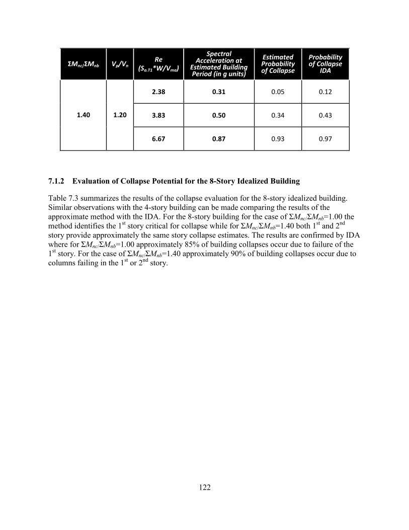
122


(Sa.T1*W/Vma)

Spectral Acceleration at

Estimated Building Period (in g units)



IDA

1.40 1.20

2.38 0.31 0.05 0.12

3.83 0.50 0.34 0.43

6.67 0.87 0.93 0.97



Similar observations with the 4-story building can be made comparing the results of the

approximate method with the IDA. For the 8-story building for the case of ΣΜnc/ΣΜnb=1.00 the

method identifies the 1st story critical for collapse while for ΣΜnc/ΣΜnb=1.40 both 1

st and 2

nd

story provide approximately the same story collapse estimates. The results are confirmed by IDA

where for ΣΜnc/ΣΜnb=1.00 approximately 85% of building collapses occur due to failure of the

1st story. For the case of ΣΜnc/ΣΜnb=1.40 approximately 90% of building collapses occur due to

columns failing in the 1st or 2

nd story.

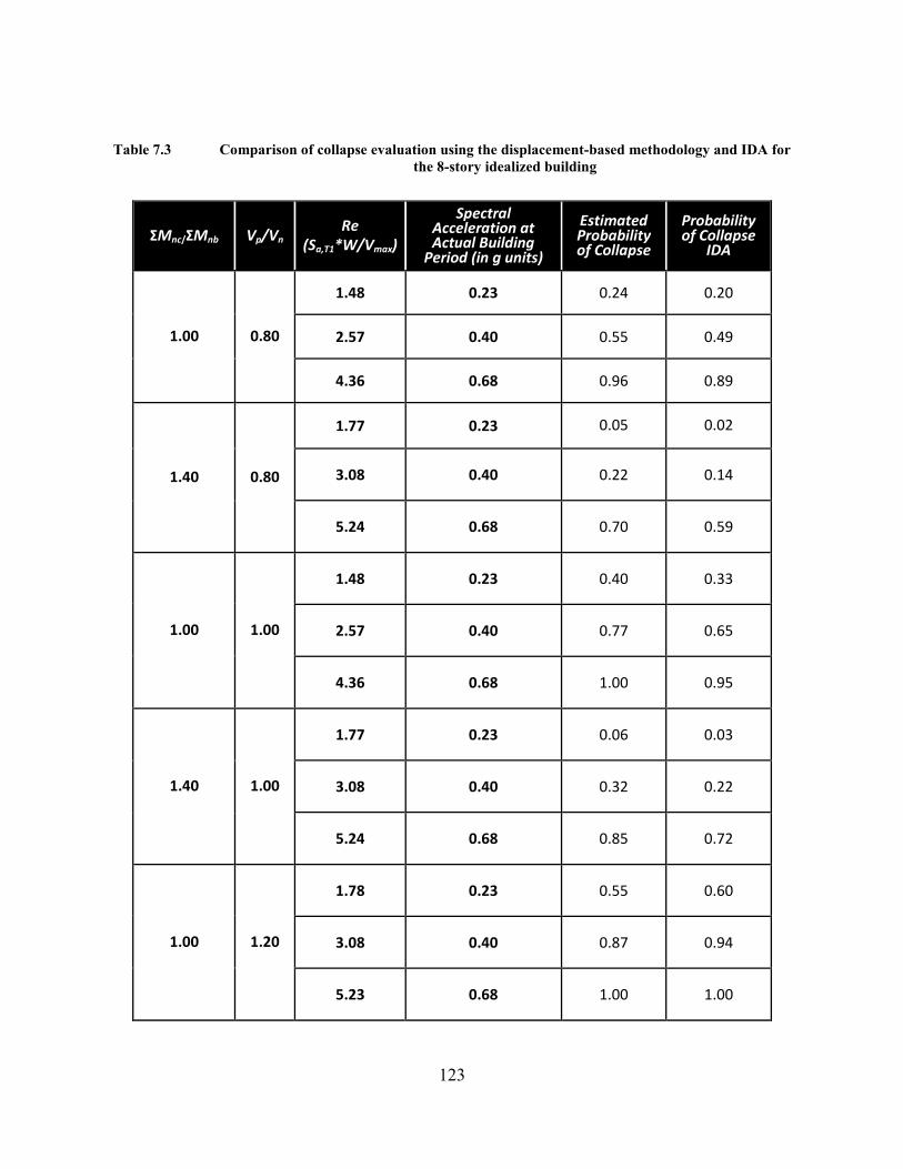
123




(Sa,T1*W/Vmax)


Period (in g units)



IDA

1.00 0.80

1.48 0.23 0.24 0.20

2.57 0.40 0.55 0.49

4.36 0.68 0.96 0.89

1.40 0.80

1.77 0.23 0.05 0.02

3.08 0.40 0.22 0.14

5.24 0.68 0.70 0.59

1.00 1.00

1.48 0.23 0.40 0.33

2.57 0.40 0.77 0.65

4.36 0.68 1.00 0.95

1.40 1.00

1.77 0.23 0.06 0.03

3.08 0.40 0.32 0.22

5.24 0.68 0.85 0.72

1.00 1.20

1.78 0.23 0.55 0.60

3.08 0.40 0.87 0.94

5.23 0.68 1.00 1.00

124


(Sa.T1*W/Vma)





IDA

1.40 1.20

1.96 0.23 0.10 0.10

3.42 0.40 0.52 0.50

5.82 0.68 0.89 0.85

Table 7.4 summarizes the results of the collapse evaluation for the 8-story idealized building

with inadequate lap splicing conditions of the column longitudinal reinforcement at the base of

the 1st story. As expected, 100% of building collapses occur due to failure of the columns at the

1st story. As explained in Chapter 6, a relatively conservative drift capacity estimate was selected

in that case. This is the main reason why the approximate method provides more conservative

collapse estimates compared to IDA although the alpha values selected were slightly less

conservative than the average alpha values observed for the critical story in IDA.

125


the 8-story idealized building with inadequate lap splicing conditions at the base of the

1st story


(Sa,T1*W/Vmax)


Period (in g units)



IDA

1.00 0.80

1.48 0.23 0.37 0.26

2.57 0.40 0.81 0.74

4.36 0.68 1.00 0.98

1.40 0.80

1.77 0.23 0.10 0.04

3.08 0.40 0.43 0.33

5.24 0.68 0.99 0.78

Table 7.5 summarizes the results of the collapse evaluation for the 8-story idealized building

with non-uniform DCRs. The latter variation of the 8-story building possesses a weak/critical

story at the mid-height (4th

story) with DCR4th=1.30DCR1st.The method identifies correctly the

4th

story as critical for collapse. In that case IDA showed that approximately 70% of building

collapses occurred due to failure of the 4th

story while the remaining 30% of collapses occurred

due to failure of the 1st or 2

nd story for the cases of ΣΜnc/ΣΜnb=0.80 and 1.20. For the case of

ΣΜnc/ΣΜnb=1.60 approximately 85% of building collapses occurred due to failure of the 4th

story.

The method again provides conservative collapse estimates with the exception of

ΣΜnc/ΣΜnb=1.60 where the method defined the alpha value of the critical story slightly lower

than what IDA provided as an average value.

126


the 8-story idealized building with weak story at the mid-height


(Sa,T1*W/Vmax)


Period (in g units)



IDA

0.80 0.80

1.65 0.23 0.24 0.21

2.86 0.40 0.61 0.57

4.87 0.68 1.00 0.95

1.20 0.80

1.88 0.23 0.06 0.05

3.26 0.40 0.42 0.39

5.54 0.68 0.87 0.82

1.60 0.80

2.37 0.23 0.01 0.02

4.12 0.40 0.20 0.27

7.01 0.68 0.60 0.71



Similar trends with the previous two buildings were observed for the 12-story building as well.

The methodology identifies the 1st story as critical for collapse for ΣΜnc/ΣΜnb=1.00, while for

ΣΜnc/ΣΜnb=1.40 the first three stories yield similar story collapse potential values. IDA showed

that for ΣΜnc/ΣΜnb=1.00 approximately 75% of the building collapses occurred due to collapse

of the 1st story . For ΣΜnc/ΣΜnb=1.40 approximately 85% of the collapse mechanisms occur due

to failure of the first three stories. Application of the approximate method for the 12-story

building yields larger errors in the collapse estimates compared to the 4 and 8-story buildings.

127

This can be explained by the higher mode effects that are not incorporated in the approximate

method.




(Sa,T1*W/Vmax)


Period (in g units)



IDA

1.00 0.80

1.02 0.18 0.03 0.02

1.70 0.30 0.38 0.29

3.11 0.55 1.00 0.88

1.40 0.80

1.19 0.18 0.01 0.01

1.98 0.30 0.02 0.01

3.62 0.55 0.45 0.35

1.00 1.00

1.02 0.18 0.09 0.06

1.70 0.30 0.59 0.47

3.11 0.55 1.00 0.92

1.40 1.00

1.19 0.18 0.01 0.01

1.98 0.30 0.11 0.04

3.62 0.55 0.66 0.53

1.00 1.20

1.22 0.18 0.23 0.20

2.04 0.30 0.70 0.61

3.73 0.55 1.00 1.00

128


(Sa.T1*W/Vma)





IDA

1.40 1.20

1.31 0.18 0.07 0.01

2.18 0.30 0.36 0.21

3.99 0.55 0.90 0.79

The tables above demonstrate that application of the approximate method correctly identifies the

critical story and provides relatively accurate collapse estimates in comparison with IDA results.

Apart from the case of buildings with uniform strength characteristics along the height, the

method was also applied for cases where inadequate lap splicing conditions exist at the base of

column members located at the 1st story and for cases where the building possessed a particularly

weak story at the mid-height. For both of these cases the approximate method was able to

identify the weak story and provide collapse estimates with relatively low error compared to

IDA. For most cases the method yielded conservative estimates of the probability of collapse

which is consistent with the way that the alpha values were selected. The results above indicate

that the method shows potential for rapid identification of hazardous concrete frame buildings;

though further verification using real older-type buildings is required before more generalized

conclusions regarding its applicability can be drawn.

129

8 Summary and Conclusions

The purpose of this study was to explore methodologies suitable for identification of seismically

hazardous reinforced concrete frame buildings. Three idealized concrete buildings were

developed for the purposes of the current study. The buildings were sequentially weakened such

that the following deficiencies were introduced: a) Weak column mechanism, b) Shear critical

columns, and c) Inadequate column bar lap splicing conditions. Consequently the collapse

potential of the buildings possessing each of the aforementioned deficiencies or combinations of

them was performed using the three evaluation methods described below:

Collapse Simulation using IDA. According to this approach Incremental Dynamic

Analysis (IDA) was used to evaluate the collapse performance of the considered

buildings. This method is considered to provide the most accurate results compared to the

other two methods presented in this study since state of the art collapse simulation tools

are employed to model the structural response. However, the method requires detailed

non-linear modeling of the considered building and multiple non-linear analyses,

rendering this approach inefficient for rapid identification of hazardous buildings.

Collapse Indicators – a Strength-Based Approach for Collapse Evaluation. This

method considered simple engineering parameters (collapse indicators) which could be

easily defined based only on hand calculations to estimate the building collapse

performance. To avoid comparison bias between buildings of different strength a

strength-based normalization parameter was employed. According to this method, an

engineer needs to estimate the values of the collapse indicator parameters and the

building strength to evaluate the building collapse performance. Although this method

seems to provide rational results it should be applied with caution for buildings with

strength characteristics different from those considered in the buildings developed in the

current study.

A Displacement-Based Approach for Collapse Evaluation. The latter method employs a

displacement-based approach that estimates drift demand and uses relationships available

in the literature to determine the drift capacity for the columns of the studied building.

After the procedure is repeated for each story, the building collapse potential can be

determined based on a comparison of the estimated demand and capacity values. This

method has the advantage that the procedure followed is not based on strength (at least

for buildings with T1>1.0 sec) and so it can be applied for a range of buildings with

different strength properties.

130

The current chapter discusses all the main conclusions that were drawn from the application of

the aforementioned methodologies as well as recommendations for further study in the future.

8.1 COLLAPSE SIMULATION

Two different models to simulate collapse were employed in the study. According to the first

model, zero-length plastic hinges were incorporated at the ends of column and beam members to

account for non-linear material response. The zero-length plastic hinges were modeled according

to Haselton et al. (2008), with some parameter updates to better reflect the characteristics of the

columns to which it was applied.

The second model used the limit state model which was developed by Elwood and Moehle

(2002). This model is capable of simulating shear and shear-induced axial failure in columns

with inadequate amount of transverse reinforcement.

Both models have been calibrated using different column databases and thus result in different

column dynamic response for the same column detailing. To evaluate the validity of both

modeling approaches, the dynamic response for eleven shaking table test structures incorporating

two different types of concrete columns was investigated. The first column type was detailed

according to the current seismic code provisions, while the second column type was detailed to

mimic older design practices. The test structures were scaled, one-bay frames consisting of two

concrete columns at opposite ends of a single bay. In some frames, both columns were ductile

columns, in other frames they were both nonductile columns, and in yet other frames a

combination of ductile and nonductile columns was used. Each frame was then subjected to one

of two different axial load levels and one of two different ground motion records.

The tested structures were analyzed using both the Elwood and Haselton models. The study

showed that the limit state material developed by Elwood tracks with sufficient accuracy the

onset of shear failure and simulates satisfactorily the dynamic response of columns with

inadequate transverse reinforcement ratio, for which it was calibrated. The plastic hinge model

calibrated by Haselton, was not as accurate as the Elwood model for columns lacking adequate

amount of transverse reinforcement and thus being flexure-shear critical. However, the Haselton

plastic hinge model reproduced with sufficient accuracy the dynamic response of columns

following modern design practice. A combination of the Haselton and Elwood model was

employed successfully for cases where the test frames consisted of columns following both old

and current design codes.

Overall, the comparison of experimental results with the two analytical models demonstrated that

the plastic hinge model calibrated by Haselton et al. represents accurately the dynamic response

of building frames consisting of columns with sufficient transverse reinforcement ratio (Vp/Vn

<0.7) and thus being flexure critical, while the limit state material is more appropriate for

building frames consisting of columns with inadequate transverse reinforcement ratio (Vp/Vn

>0.7) and thus being shear critical.

After exploring the validity of collapse simulation techniques using shaking table tests, the

Elwood and Haselton models were used to simulate the collapse response of idealized concrete

frame buildings developed for the purposes of this study. The idealized buildings were initially

131

designed according to current seismic code provisions. Consequently the performance of

variations of the idealized buildings was explored including one or more structural deficiencies

indicative of older design practice (weak column story mechanisms, columns with inadequate

transverse reinforcement, and inadequate column bar lap splicing conditions). As explained

above, it was decided to use the Haselton model to simulate the response of code complying

column and beam members, while the Elwood model was used to simulate the response of

buildings which consisted of column members with inadequate transverse reinforcement.

Collapse evaluation was performed using Incremental Dynamic Analysis. According to this

method, a set of far–fault ground motions was scaled until the structure reaches collapse. Using

statistical post-processing of the results, curves linking earthquake intensity with probability of

collapse were derived.

Evaluation of building performance using results from numerous collapse simulations is

considered today to be one of the most accurate methods to estimate building collapse

performance. Thereby, the IDA results obtained from collapse simulations were used to calibrate

the two approximate methods presented below, which are more efficient for rapid identification

of seismically hazardous concrete buildings

8.2 COLLAPSE INDICATORS – A STRENGTH-BASED APPROACH FOR

COLLAPSE EVALUATION

In Chapter 5 a study was performed to explore the effect of two simple engineering parameters,

termed as collapse indicators, in the collapse potential of concrete frame structures. The collapse

indicators selected constitute key concepts of the capacity design principles of modern seismic

codes. According to the results of this study, both the column-to-beam bending moment strength

ratio and the plastic shear capacity over the required shear demand exhibit strong correlation

with the collapse potential.

As expected, the increase of beam-to-column bending moment strength ratio leads to

concentration of damage in one story and consequently to lateral instability. Conversely decrease

of the value of this ratio allows a better distribution of damage over the height of the building

with beams failing first. For regular frames of the type considered in this study, having

reasonable values of the variable ΣMnc/ΣMnb, beam yielding mechanisms do not extend full

height but instead are concentrated in the lower stories. For the case of ΣMnc/ΣMnb = 1.2 about

25-30% of the building height participates in the collapse mechanism while for the case of

ΣMnc/ΣMnb =1.6 the percentage increases to 30-60%.

The decrease in the amount of transverse reinforcement results in decrease of the column shear

strength. This corresponds to an increase in the column flexural demand over capacity ratio,

Vp/Vn. For all other variables being the same, the collapse probability increases with increasing

values of the variable Vp/Vn, that is, as columns become increasingly shear-critical.

Finally the study demonstrated that all parameters explored, ΣMnc/ΣMnb and Vp/Vn, interact, such

that it is necessary to consider the combination of variables in order to quantify the probability of

collapse. To avoid comparison bias for buildings having different strength two normalization

factors, Re and M, based on base shear capacity were employed.

132

At Appendix E, tables with the input parameters ΣMnc/ΣMnb, Vp/Vn, Re and M are provided to

estimate the building collapse potential.

8.3 A DISPLACEMENT-BASED APPROACH FOR COLLAPSE EVALUATION

A displacement based approach was developed in Chapter 6. This approach requires the engineer

to select the level of seismic hazard and then use an equivalent Single Degree of Freedom

(SDOF) system to estimate story drift demand. The procedure followed in this chapter is

considered more rational than the one presented in Chapter 5, since collapse is mainly occurring

due to inability of one or more structural members to accommodate excessive drifts/deformation

demands.

One of the main advantages of this procedure is that for buildings with period T1>1.0 sec, the

application of the method was shown to be independent of the building strength which could

vary for different considered buildings. Another advantage is that since both drift demand and

drift capacity can be quantified in a probabilistic framework, a simple mathematical formulation

that can accommodate both uncertainty in the drift demand and uncertainty in the drift capacity

is possible.

Chapter 7 deployed the displacement-based approach of Chapter 6 to estimate the collapse risk

of the various buildings studied in the course of this work. The procedure described in Chapter 6

was shown to correctly identify the weakest stories of the considered buildings and estimate with

sufficient accuracy the building collapse potential. The accuracy of the results was evaluated

using the results obtained from collapse simulation studies presented in Chapters 4 and 5. Taking

into account both the accuracy and the efficiency in application, the displacement based method

was overall shown to be the most appropriate method for rapid identification of seismically

hazardous concrete buildings.

133

8.4 RECOMMENDATIONS FOR FUTURE STUDY

Although the proposed methodologies were successful in estimating building collapse risk,

further work needs to be done in order to explore the effect of some additional deficiencies and

structural systems that have not been considered in the current study. Some of the most common

cases of systems and deficiencies that need to be investigated in order to be able to use the

proposed methodology for a wide range of existing buildings would be:

Column-slab frames. Many older-type concrete building include frames with no beams

or girders. Instead, flat slabs act to transfer the lateral forces to the column members. In

such cases, excessive drift due to seismic forces can cause punching shear failure. A

number of laboratory tests performed for slab-column connections with and without shear

reinforcement could be used to derive probabilistic capacity models.

Building with structural walls. A significant number of older concrete buildings include

either lightly confined concrete walls or masonry infill walls confined by structural

beams and columns. The presence of walls would alter significantly the assumed drift

profiles, while failure of a wall would lead to increased drift or even loss of vertical

support. Drift pattern profiles need to be developed for buildings with structural systems

that consist of a combination of walls and frames. An important issue in that case would

be modeling the sudden strength and stiffness degradation of lightly reinforced concrete

walls and how this affects the drift demands and eventually the progressive collapse of

the building.

Plan irregularities. The current study did not consider the effect of plan irregularity in

creating torsional moments and thus, increase in the inter-story drift demands. A

magnification factor for drift demand could be calibrated using three dimensional

analyses.

Unconfined beam column joints. A structural deficiency very commonly observed in

older-type buildings is beam-column connections without joint transverse reinforcement.

Several laboratory tests have been conducted for both interior and exterior joints.

Although there have not been adequate physical evidence of building collapses triggered

by joint failures, severe joint damage has been reported in past earthquakes. The effect of

joints on both the demand and capacity estimates should be incorporated using the

available experimental data.

This study considered data from a large number of non-linear dynamic analyses to develop

profiles of story drift patterns as a function of the spectral acceleration. The input parameter

(spectral acceleration) and predicted variable (story drift patterns) were assumed to be related in

a linear way. The coefficient linking this two variables, ax, was estimated through minimizing the

sum of squared errors. The large dispersion observed indicates that the assumed model might not

be the ideal model to relate the two aforementioned variables. A more in-depth statistical

procedure should be followed to reduce the observed dispersion between observed and predicted

values in the story drift demands. This would lead to a more accurate approximation of the

building collapse potential.

The methodologies presented have been calibrated by using, in most cases, idealized buildings

with uniform structural parameters values such that varying the value of each parameter could be

directly linked to collapse potential. Although this approach is appealing due to its simplicity, it

134

may oversimplify response of actual buildings in which structural parameters can be significantly

non-uniform within the same story and from story to story. Therefore, the proposed

methodologies needs to be further verified using examples of existing older-type concrete

buildings.

The presented collapse evaluation methodologies could be incorporated as a part of a holistic risk

assessment approach that should be followed in a regional level. Cost-benefit analysis principles

towards optimal risk management should be applied when forming seismic policy to classify

buildings as particularly hazardous, moderately hazardous, and slightly hazardous. It is suggested

that since human loss is difficult to quantify in financial terms, life safety standards for collapse

prone buildings could be established using risk metrics and recovery costs that can be directly

compared with other routine hazards like car accidents or plane crashes. Unnecessary

conservatism in classifying earthquake hazardous buildings introduces increased financial

burden to building owners or authorities. Communities that implement plans using such a

methodology would become more resilient, enabling them to recover from future disasters.

135

REFERENCES

ACI, (2008), “Guide to Durable Concrete”, ACI 201R-08, American Concrete Institute,

Farmington Hills, Michigan.

ACI,( 2011), “Building Code Requirements for Structural Concrete and Commentary”, ACI

318-11, American Concrete Institute, Farmington Hills, Michigan.

ASCE,( 2003), “Seismic Evaluation of Existing Buildings”, ASCE/SEI 31-03, American Society

of Civil Engineers, Structural Engineering Institute, Reston, Virginia.

ASCE, (2006), “Seismic Rehabilitation of Existing Buildings”, ASCE/SEI 41-06, Including

Supplement No. 1, American Society of Civil Engineers, Structural Engineering Institute,

Reston, Virginia.

ASCE, (2010), “Minimum Design Loads for Buildings and Other Structures”, ASCE/SEI 7-10,

American Society of Civil Engineers, Structural Engineering Institute, Reston, Virginia.

ASCE, (2013), “Seismic Evaluation and Retrofit of Existing Buildings”, ASCE/SEI 41-13,

American Society of Civil Engineers, Structural Engineering Institute, Reston, Virginia.

ATC, (2013), “Evaluation of the Methodology to Select and Prioritize Collapse Indicators in

Older Concrete Buildings”, ATC-78-1 Report, Applied Technology Council, Redwood

City, California.

ATC, (2014), “Seismic Evaluation for Collapse Potential of Older Concrete Frame Buildings”,

ATC-78-2, Applied Technology Council, Redwood City, California.

Baker, J., (2007), “Probabilistic Structural Response Assessment Using Vector-Valued Intensity

Measures”, Earthquake Engineering and Structural Dynamics, Vol. 36, p. 1861-1883

136

Berry, M., Parrish, M., and Eberhard, M., (2004), “PEER Structural Performance Database

User’s a ual”, Pacific Earthquake Engineering Research Center, University of

California, Berkeley, California, last accessed September 26, 2013, Available at

http://nisee.berkeley.edu/spd/ and http://maximus.ce.washington.edu/~peera1.

Blume, J.A., Newmark, N.M., and Corning, L.M., (1961), “Design of Multi-story Reinforced

Concrete Buildings for Earthquake Motions”, Portland Cement Association, Chicago,

Illinois.

Concrete Coalition, (2013), Online Database, Sponsored by the Earthquake Engineering

Research Institute, the Pacific Earthquake Engineering Research Center, and the Applied

Technology Council, Oakland, California, http://www.concretecoalition.org

DeBock, D.J., Liel, A.B., Haselton, C.B., Hooper, J.D., and Henige, R.A., (2014), “Importance

of seismic design accidental torsion requirements for building collapse capacity”,

Earthquake Engineering and Structural Dynamics, Vol. 43, Issue 6, p. 831-850

Ellingwood, B., Galambos, T.V., MacGregor, J.G., and Cornell, C.A., (1980), “Development of a

Probability Based Load Criterion for American National Standard A58”, Special

Publication No. 577, National Bureau of Standards, Washington, D.C.

Elwood, K.J., (2002), “Shake Table Tests and Analytical Studies on the Gravity Load Collapse

of Reinforced Concrete Frames”, Ph.D. Dissertation, University of California, Berkeley

Elwood, K.J., (2004), “Modelling failures in existing reinforced concrete columns, Canadian

Journal of Civil Engineering”, Vol. 31, No. 5, pp. 846-859.

Elwood, K.J., Matamoros, A., Wallace, J.W., Lehman, D.E., Heintz, J.A., Mitchell, A., Moore,

M.A., Valley, M.T., Lowes, L. Comartin, C., and Moehle, J.P., (2007), “Update of

ASCE/SEI 41 Concrete Provisions, Earthquake Spectra”, Vol. 23, No. 3, pp. 493-523.

FEMA, (1998), “Evaluation of Earthquake Damaged Concrete and Masonry Wall Buildings”,

FEMA 306, Federal Emergency Management Agency, Washington, D.C.

FEMA, (2000), “Prestandard and Commentary for the Seismic Rehabilitation of Buildings”,

FEMA 356 Report, prepared by the Applied Technology Council, under contract to the

Building Seismic Safety Council, for the Federal Emergency Management Agency,

Washington, D.C.

FEMA, (2009), “Quantification of Building Seismic Performance Factors”, FEMA P-695,

prepared by the Applied Technology Council for the Federal Emergency Management

Agency, Washington, D.C.

http://www.concretecoalition.org/

137

Galanis P., and Moehle, J.P., (2014), “Development of Collapse Indicators for Older-Type

Reinforced Concrete Buildings”, 15th

WCEE, September 24-28 2012, Lisbon, Portugal

Galanis P., and Moehle, J.P., (2014), “Development of Collapse Indicators for Seismic Risk

Assessment of Older-Type Reinforced Concrete buildings”, Earthquake Spectra, (in-

press), http://dx.doi.org/10.1193/080613EQS225M

Galanis P., and Moehle, J.P., (2014), “Development of Collapse Indicators for Seismic Risk

Assessment of Older-Type Reinforced Concrete buildings”, UCB/SEMM Report

2014/03, http://nisee.berkeley.edu/documents/SEMM/SEMM-2014-03.pdf

Galanis P., Shin Y.P. and Moehle, J.P., (2014), “Modeling the Dynamic Structural Behavior of

Ductile and Non-Ductile Reinforced Concrete Frames”, 10th

NCEE, July 21-25 2014,

Alaska

Goel, R., and Chopra, A.K., (1997), “Vibration Properties of Buildings Determined from

Recorded Earthquake Motions”, UCB/EERC-97/14, Earthquake Engineering Research

Center, University of California, Berkeley, California.

Ghannoum, W.M., and Matamoros, A.B., (2013), “Nonlinear Modeling Parameters and

Acceptance Criteria for Concrete Columns”, Submitted for publication in ACI Special

Publications, American Concrete Institute, Farmington Hills, Michigan.

Haselton, C., Liel, A., Lange, S.T., and Deierlein, G.G.,(2008), “Beam-Column Element Model

Calibrated for Predicting Flexural Response Leading to Global Collapse of RC Frame

Buildings”, PEER Report, 2007/03

Hassan, W.M. , Moehle, J.P. (2012), “A Cyclic Nonlinear Macro Model for Numerical

simulation of Beam-Column Joints in Existing Concrete Buildings”, 15th

WCEE,

September 24-28 2012, Lisbon, Portugal

Hassan, W.M. , Moehle, J.P. (2013), “Quantification of Residual Axial Capacity of Beam-

Column Joints in Existing Concrete Buildings under Seismic Load Reversals”,

COMPDYN, 4th

ECCOMAS Thematic Conference on Computational Methods in

Structural Dynamics and Earthquake Engineering, 12-14 June 2013, Kos island, Greece

Henkhaus, K., (2010), “Axial Failure of Vulnerable Reinforced Concrete Columns Damaged by

Shear Reversals”, Ph.D. Dissertation, Purdue University, West Lafayette, Indiana.

Ibarra, L. F., and Krawinkler, H. (2005). “Global collapse of frame structures under seismic

excitations,” Technical Report 152, The John A. Blume Earthquake Engineering

Research Center, Department of Civil Engineering, Stanford University, Stanford, CA.

http://dx.doi.org/10.1193/080613EQS225M

http://nisee.berkeley.edu/documents/SEMM/SEMM-2014-03.pdf

138

Ibarra, L. F., Medina, R. A., and Krawinkler, H. (2005). “Hysteretic models that incorporate

strength and stiffness deterioration,” Earthquake Engineering and Structural Dynamics,

Vol. 34, 12, pp. 1489-1511.

ICBO, (1976), “Uniform Building Code”, International Council of Building Officials, Whittier,

California.

Li, Y., Elwood K.J., and Hwang S.-J., (2013), “Assessment of ASCE/SEI 41 Concrete Column

Provisions using Shaking Table Tests”, Submitted for publication in ACI Special

Publications, American Concrete Institute, Farmington Hills, Michigan.

Luco, N., Mori, Y., Funahashi, Y., Cornell, C.A., and Nakashima, M., (2003), “Evaluation of

Predictors of Non-Linear Seismic Demands using "Fishbone" Models of SMRF

Buildings, Earthquake Engineering and Structural Dynamics”, Vol. 32, No. 14, pp.

2267-2288.

Lynn, A. C., Moehle, J. P., Mahin, S. A., and Holmes, W. T. (1996), “Seismic Evaluation of

Existing Reinforced Concrete Columns”, Earthquake Spectra, Earthquake Engineering

Research Institute, Vol. 12, No. 4, November 1996, pp. 715-739

Melchers, R.E., (1999), “Structural Reliability Analysis and Prediction”, Second Edition, John

Wiley and Sons Ltd., West Sussex, England.

Melek, M.,and Wallace, J.W., (1999), “Cyclic Behavior of Columns with Short Lap Splices”,

ACI Structural Journal, Vol. 101, pp. 802-811.

Nakashima, M.,Ogawa K. and Inoue, K., (2002), “Generic Frame Model Simulation of

Earthquake Responses of Steel Moment Frames”, Earthquake Engineering and Structural

Dynamics, Vol. 31, pp. 671-692.

NEES, (2010), Grand Challenge Research Project, “Mitigation of Collapse Risks in Older

Reinforced Concrete Buildings”, George E. Brown Network for Earthquake Engineering

Simulation, http://peer.berkeley.edu/grandchallenge/index.html,

NIST, (2010a), “Concrete Model Building Subtypes Recommended for Use in Collecting

Inventory Data”, NIST GCR 10-917-6, prepared by the Building Seismic Safety Council

for the National Institute of Standards and Technology, Gaithersburg, Maryland.

NIST, (2010b), “Evaluation of the FEMA P-695 Methodology for Quantification of Building

Seismic Performance Factors”, NIST GCR 10-917-8, prepared by the NEHRP

Consultants Joint Venture, a partnership of the Applied Technology Council and

Consortium of Universities for Research in Earthquake Engineering, for the National

Institute of Standards and Technology, Gaithersburg, Maryland.

http://peer.berkeley.edu/grandchallenge/index.html

139

NIST, (2010c), “Program Plan for the Development of Collapse Assessment and Mitigation

Strategies for Existing Reinforced Concrete Buildings”, NIST GCR 10-917-7, prepared

by the NEHRP Consultants Joint Venture, a partnership of the Applied Technology

Council and Consortium of Universities for Research in Earthquake Engineering, for the

National Institute of Standards and Technology, Gaithersburg, Maryland.

Park, S. and Mosalam, K. , (2013), “Simulation of Reinforced Concrete Frames with Nonductile

Beam-Column Joints”, EERI Spectra, Vol. 29, pp. 233-257

Renouard, F. (2014), “Evaluation Methodology to Assess the Collapse of Older Reinforced

Concrete Buildings”, Master of Science Thesis (in-press)

Sattar, S. (2013), “Influence of Masonry Infill Walls and Other Building Characteristics on

Seismic Collapse of Concrete Frame Buildings”, Ph.D. Dissertation, University of

Colorado, Boulder.

Sezen, H. (2002), “Seismic Behavior and Modeling of Reinforced Concrete Building Columns”,

Ph.D. Dissertation, University of California, Berkeley.

Shin, Y. B. (2007), “Dynamic Response of Ductile and Non-Ductile Reinforced Concrete

Colum s”, Ph.D. Dissertation, University of California, Berkeley.

Shome N. (1999), “Probabilistic Seismic Demand Analysis of Nonlinear Structures”, Ph.D.

Dissertation, Stanford University

Smith, W. (2005), “The Challenge of Earthquake Risk Assessment”, Seism. Res. Lett., Vol. 76,

p. 415-416

USGS, (2008), “Earthquake Hazard Maps”, United States Geological Survey, Reston, Virginia,

http://earthquake.usgs.gov/hazards/products/conterminous/2008/maps/

Vamvatsikos, D. and Cornell, C.A., (2004), “Applied Incremental Dynamic Analysis”,

Earthquake Spectra, Vol. 20, No. 2, p.523-553

Wang, Z., (2006), “Understanding Seismic Hazard and Risk Assessment: A Gap between

Engineers and Seismologists”, Proceedings, 14th

World Conference on Earthquake

Engineering, October 12-17 2008, Beijing, China.

Woods, C., and Matamoros, A., (2010), “Effect of Longitudinal Reinforcement Ratio on the

Failure Mechanism of R/C Columns Most Vulnerable to Collapse”, Proceedings, The 9th

U.S. National Conference and 10th Canadian Conference on Earthquake Engineering,

Toronto, Canada.

http://earthquake.usgs.gov/hazards/products/conterminous/2008/maps/

140

Yosimura, M.,Nakamura, T. (2002), “Intermediate-Story Collapse of Co rete Buildi gs”,

Proceedings of the Third U.S. – Japan Worksop on Performance Based Eaarthquake

Engineering Methodology for Reinforced Concrete Building Structures, August 16-18,

2001, Seattle, Washington, 107-118

141

A. Design Parameters of the Idealized Buildings

The current section presents details regarding the design of the three (4, 8, and 12 –story)

idealized buildings that were considered in the current study.

As mentioned in Chapter 4, all the considered archetype buildings were designed such that they

correspond to regular concrete frame buildings. The archetype buildings have a rectangular plan

with five bays in each direction without plan torsion. The structural system consists of reinforced

concrete frames without any infill or structural walls. The archetype buildings for each category

were designed to have proportions and force-deformation characteristics similar to those of new

buildings. More specifically the detailing of archetype buildings satisfies ACI 318-11 code

requirements, except Σ Σ 1.0⁄ at every joint except the roof level (Σ = sum of

nominal moment strengths of columns at a beam-column joint and Σ = sum of nominal

moment strengths of beams at the same joint).

Consequently the structural properties of the archetype buildings were varied and structural

deficiencies were introduced somewhat typical of those found in older buildings.

The design base-shear of the archetype buildings was set at approximately 0.10*W, where W is

the effective seismic weight of the building.

DESIGN PHILOSOPHY OF ARCHETYPE BUILDINGS A.1.

Although the prototype buildings vary in height they have similar building geometry, depicted in

Figure A.1. The buildings have square plan shape with five bays in each principal direction. All

frames were designated as seismic-force-resisting frames and designed to carry appropriate

earthquake and gravity loading according to the corresponding tributary area.

Only the interior frames were modeled, using a two dimensional method, because interior frames

support larger tributary area and therefore have larger column loads. This causes interior frames

to be more vulnerable to shear induced axial load failure that is typical in older-type buildings.

Thus, the design parameters and drawings only of the interior frame are presented.

142

Figure A.1 Three- dimensional view of the studied buildings (for clarity of presentation, only

the perimeter frames are shown)

DESIGN ASSUMPTIONS A.2.

A.2.1 Applied Loads

Dead Load: 150 psf ( includes the self-weight )

Cladding: 15 psf

Live Load: 60 psf

The tributary width for the gravity loads is 10 feet

The lateral load design for inverted triangular load with design base-shear strength of

0.10W, where W is the effective seismic weight resisted by each frame

143

A.2.2 Material Properties

Reinforced Concrete characteristic strength f’c 3000psi 3 ksi

Steel Reinforcement Grade 60 – fy=60000 psi = 60 ksi

Reinforced Concrete modulus of Elasticity Ec=3122 ksi

Steel Reinforcement modulus of Elasticity Es=29000 ksi

A.2.3 Calculation of Loads

The tributary width for the interior frame is (10+12) ft = 22 ft. The selected frame is shown in

Figure A.2 .

Distributed Dead Load per floor: wdead=150 psf *22 ft = 3300 pounds/ft = 3.30 kips/ft

Distributed Live Load per floor: wlive=60 psf *22 ft = 1320 pounds/ft = 1.32 kips/ft

Figure A.2 Plan view of the archetype idealized buildings

144

A.2.4 Strength Requirements

All designs follow the strength design procedure of ACI 318-11, except the design load

combinations, including seismic, were modified. The following specific procedures were used.

Designs were checked for the following load combinations, with Static_1 and EQ_1

controlling the designs:

o 1.2*D + 1.6*L (Static 1)

o 1.4*D (Static 2)

o 1.0*D+0.25*L ±1.0*E (EQ_1)

o 0.9*D ±1.0*E (EQ_2)

, where D = dead load, L = live load, and E = earthquake load.

The earthquake loading considered for the member design in combinations EQ_1 and

EQ_2 was assumed to be equal to 10% of the effective seismic building weight uniformly

for all the archetype buildings.

Member moment design strengths, Md, were set equal to moment demands obtained from

design load combinations including gravity and seismic loads, and then nominal moment

strengths, Mn, were defined as Mn = a1Md/φ ; φ is a resistance factor for tension-

controlled members, from ACI 318-11, such that φ= 0.90; a1 is a modification factor to

increase strength due to section oversizing, such that a1 = 1.15. For each value of Mn =

a1Md/φ, the required longitudinal reinforcement was determined. If the reinforcement was

less than the building code minimum (ACI 318-11), code minimum values were assigned.

Finally, effective yield strength for nonlinear analysis was increased to a2 Mn in which a2

is a modification factor to increase strength due to material overstrength, such that, a2 =

1.15.

Transverse reinforcement was selected for every column so that the target value of Vp/Vn

was obtained, where Vn corresponds to the shear strength of each column calculated

according to ASCE/SEI 41 (ASCE/SEI, 2006) and Vp is the plastic shear demand

(controlled by flexure). For the archetype buildings Vp/Vn ratio was selected to be equal to

Vp/Vn=0.6. The spacing of transverse reinforcement for the beams in all the buildings

was selected to be equal to d/2, where d is the beam effective depth.

Beam-column joints were not considered in the design. It is likely that some of the joint

dimensions did not meet current code requirements; however, joint failure was not

considered in this study.

145

DIMENSIONS AND REINFORCEMENT FOR ARCHETYPE BUILDINGS A.3.

To be able to define the moment-rotation behavior for flexural response, the shear failure surface

for shear response, and the axial failure surface for axial response, it was considered necessary to

select indicative reinforcement that approximated reinforcement that would be required for the

design seismic forces.

A.3.1 4-Story Archetype Building

Figure A.3 illustrates an elevation view of the 4-story archetype building.

Figure A.3 Schematic elevation view of the 4-story archetype building

The reinforcement schedules of the column and beam members for the 4-story building are

provided in Tables A.1-3.

Table A.1 Interior column reinforcement schedule of the 4-story archetype building

Level Dimensions Longitudinal

Reinforcement ρlong

Transverse Reinforcement

ρtransverse

1 18"x18" 12#8 0.029 #3/3.7" (3-legs) 0.0050

2 18"x18" 10#8 0.024 #3/2.8" (3-legs) 0.0065

3 18"x18" 10#7 0.019 #3/3.4" (3-legs) 0.0054

4 18"x18" 8#7 0.015 #3/4.4" (3-legs) 0.0042

146

Table A.2 Corner column reinforcement schedule of the 4-story archetype building




ρtransverse

1 16"x16" 8#7 0.019 #3/6.5" (3-legs) 0.0032

2 16"x16" 8#7 0.019 #3/4.7" (3-legs) 0.0044

3 16"x16" 8#7 0.019 #3/4.6" (3-legs) 0.0045

4 16"x16" 8#7 0.019 #3/4.5" (3-legs) 0.0046

Table A.3 Beam reinforcement schedule of the 4-story archetype building

Level Dimensions Longitudinal Reinforcement

ρlong Transverse

Reinforcement ρtransverse

Top Bottom

1 16"x24" 6#7 3#7 0.014 #3/10" (2-legs) 0.0014

2 16"x24" 5#7+1#6 3#7 0.014 #3/10" (2-legs) 0.0014

3 16"x24" 5#7+1#6 2#7+1#6 0.013 #3/10" (2-legs) 0.0014

4 16"x24" 4#7 2#7 0.0095 #3/10" (2-legs) 0.0014



147








ρtransverse

1 22"x22" 14#9 0.029 #3/4.0" (4-legs) 0.0050

2 22"x22" 4#9+6#8 0.018 #3/3.1" (4-legs) 0.0065

3 20"x20" 4#9+4#8 0.018 #3/3.4" (4-legs) 0.0065

4 20"x20" 10#9 0.021 #3/2.7" (4-legs) 0.0081

5 18"x18" 4#9+6#8 0.027 #4/4.4" (4-legs) 0.0076

6 18"x18" 4#9+4#8 0.022 #4/4.6" (4-legs) 0.0072

7 18"x18" 4#9+4#8 0.022 #4/5.3" (4-legs) 0.0063

8 18"x18" 4#9 0.012 #4/3.8" (4-legs) 0.0048

148





ρtransverse

1 18"x18" 4#7+4#6 0.013 #3/5.6" (3-legs) 0.0032

2 18"x18" 4#7+4#6 0.013 #3/3.6" (3-legs) 0.0051

3 18"x18" 8#7 0.015 #3/3.6" (3-legs) 0.0051

4 18"x18" 8#7 0.015 #3/3.9" (3-legs) 0.0047

5 16"x16" 8#7 0.019 #3/4.8" (3-legs) 0.0043

6 16"x16" 8#7 0.019 #3/4.9" (3-legs) 0.0042

7 16"x16" 8#7 0.019 #3/5.7" (3-legs) 0.0036

8 16"x16" 8#6 0.014 #3/6.6" (3-legs) 0.0031



ρlong Transverse


Top Bottom

1 18"x26" 4#8+4#7 3#7+1#6 0.017 #4/11" (2-legs) 0.002

2 18"x26" 4#8+4#7 3#7+1#6 0.017 #4/11" (2-legs) 0.002

3 18"x26" 4#8+4#7 3#7+1#6 0.017 #4/11" (2-legs) 0.002

4 18"x26" 4#8+4#7 3#7+1#6 0.017 #4/11" (2-legs) 0.002

5 16"x24" 3#7+2#6 2#7 0.01 #4/10" (2-legs) 0.0025

6 16"x24" 3#7+2#6 2#7 0.01 #4/10" (2-legs) 0.0025

7 16"x24" 3#7+2#6 2#7 0.01 #4/10" (2-legs) 0.0025

8 16"x24" 3#7+2#6 2#7 0.01 #4/10" (2-legs) 0.0025



149




150





ρtransverse

1 26"x26" 18#9 0.027 #3/3.2" (4-legs) 0.0053

2 26"x26" 12#8 0.014 #3/3.0" (4-legs) 0.0056

3 26"x26" 6#9+6#8 0.016 #3/2.4" (4-legs) 0.0071

4 24"x24" 6#9+6#9 0.019 #3/2.8" (4-legs) 0.0065

5 24"x24" 8#9+4#8 0.019 #3/2.7" (4-legs) 0.0066

6 22"x22" 8#9+4#8 0.023 #3/3.0" (4-legs) 0.0067

7 22"x22" 6#9+6#8 0.022 #3/2.6" (4-legs) 0.0077

8 20"x20" 6#9+6#8 0.027 #3/3.0" (4-legs) 0.0073

9 20"x20" 4#9+6#8 0.022 #3/2.9" (4-legs) 0.0076

10 20"x20" 12#8 0.024 #3/3.2" (4-legs) 0.0069

11 20"x20" 4#8+8#7 0.020 #3/3.6" (4-legs) 0.0061

12 20"x20" 4#8+4#7 0.014 #3/4.1" (4-legs) 0.0054

151





ρtransverse

1 20"x20" 4#8+4#7 0.014 #3/3.7" (3-legs) 0.0045

2 20"x20" 4#8+4#7 0.014 #3/4.1" (3-legs) 0.0040

3 20"x20" 4#9+4#8 0.018 #3/4.1" (3-legs) 0.0040

4 18"x18" 4#9+4#8 0.022 #3/2.9" (3-legs) 0.0063

5 18"x18" 4#9+4#8 0.022 #3/2.9" (3-legs) 0.0063

6 18"x18" 4#9+4#8 0.022 #3/3.0" (3-legs) 0.0061

7 18"x18" 8#8 0.020 #3/3.3" (3-legs) 0.0056

8 18"x18" 8#8 0.020 #3/3.7" (3-legs) 0.0050

9 18"x18" 4#8+4#7 0.017 #3/4.3" (3-legs) 0.0043

10 16"x16" 4#8+4#7 0.022 #3/5.3" (3-legs) 0.0035

11 16"x16" 8#7 0.019 #3/6.3" (3-legs) 0.0029

12 16"x16" 4#7+4#6 0.016 #3/6.7" (3-legs) 0.0027

152



ρlong Transverse


Top Bottom

1 20"x28" 8#8 2#8+2#7 0.016 #4/12" (2-legs) 0.0017

2 20"x28" 8#8 2#8+2#7 0.016 #4/12" (2-legs) 0.0017

3 20"x28" 6#8+3#7 2#8+2#7 0.017 #4/12" (2-legs) 0.0017

4 18"x26" 4#8+3#7 2#8+2#7 0.017 #4/11" (2-legs) 0.002

5 18"x26" 8#8 1#8+3#7 0.019 #4/11" (2-legs) 0.002

6 18"x26" 4#8+4#7 4#7 0.017 #4/11" (2-legs) 0.002

7 18"x26" 2#8+6#7 3#7+1#6 0.016 #4/11" (2-legs) 0.002

8 18"x26" 8#7 3#7+1#6 0.015 #4/11" (2-legs) 0.002

9 18"x26" 8#7 3#7 0.015 #4/11" (2-legs) 0.002

10 16"x24" 6#7 3#7 0.014 #4/10" (2-legs) 0.0025

11 16"x24" 5#7 3#7 0.013 #4/10" (2-legs) 0.0025

12 16"x24" 4#7 3#7 0.011 #4/10" (2-legs) 0.0025

BUILDING MODEL VARIATIONS OF ARCHETYPE BUILDINGS A.4.

As mentioned in section A.2.4 for the archetype buildings the transverse reinforcement ratio was

selected such that Vp/Vn=0.6 uniformly for all column members of the considered buildings. The

archetype building models were sequentially weakened by modifying transverse reinforcement

and column to beam bending moment strength ratio to test the sensitivity of collapse

performance to these parameters.

The modification of beam bending moment strength ratio was performed by decreasing the

bending moment strength of the beam members but leaving their member dimensions the same

(this change is equivalent to modifying the longitudinal transverse reinforcement ratio).

The modification of transverse reinforcement ratio was performed such that the parameter Vp/Vn

equals 0.8, 1.0 and 1.2 uniformly for all the column members (the Vp/Vn ratio of beam members

was not modified).

153

In the section below, the reinforcement and modeling details for variations of the considered

archetype buildings for Vp/Vn=0.6 (Archetype building), 0.8,1.0 and 1.2 are provided.

A.4.1 4-Story Building Column Transverse Reinforcement Variations

Details regarding the transverse reinforcement and modeling parameters of the column members

for the 4-story building are provided in Tables A.10-13.

Table A.10 Reinforcement and modeling parameter details of the 4-story building for the case of

Vp/Vn=0.6 (Archetype 4-story building)

Dimensions spacing (in) Ast,transv

(in2) ρsh Vn(ASCE41) Vp/Vn θcap,

pl θpc λ

1st Story

Interior 18"x18" 3.70 0.33 0.0050 112.47 0.60 0.049 0.083 79.32

Corner 16"x16" 6.50 0.33 0.0032 59.95 0.60 0.052 0.096 56.33

2nd Story

Interior 18"x18" 2.80 0.33 0.0065 128.68 0.60 0.062 0.100 98.12

Corner 16"x16" 4.70 0.33 0.0044 71.33 0.60 0.062 0.100 77.94

3rd Story

Interior 18"x18" 3.40 0.33 0.0054 108.82 0.60 0.062 0.100 97.04

Corner 16"x16" 4.60 0.33 0.0045 70.87 0.60 0.064 0.100 81.12

4th Story

Interior 18"x18" 4.40 0.33 0.0042 87.29 0.60 0.060 0.100 90.51

Corner 16"x16" 4.50 0.33 0.0046 69.97 0.60 0.067 0.100 84.89


Vp/Vn=0.8

Dimensions spacing (in) Ast,transv (in

2) ρsh Vn(ASCE41) Vp/Vn Drshear,Elwood

1st Story Interior 18"x18" 6.70 0.33 0.0027 83.72 0.80 0.029

Corner 16"x16" 12.00 0.33 0.0017 45.05 0.80 0.031

2nd Story Interior 18"x18" 4.50 0.33 0.0041 96.62 0.80 0.035

Corner 16"x16" 7.60 0.33 0.0027 54.18 0.80 0.034

3rd Story Interior 18"x18" 5.60 0.33 0.0033 81.37 0.80 0.034

Corner 16"x16" 7.60 0.33 0.0027 52.74 0.80 0.035

4th Story Interior 18"x18" 7.30 0.33 0.0025 65.83 0.80 0.034

Corner 16"x16" 7.20 0.33 0.0029 52.37 0.80 0.036

154


Vp/Vn=1.0




Corner 16"x16" 11.00 0.15 0.0008 36.07 1.00 0.027


Corner 16"x16" 12.50 0.33 0.0017 43.29 1.00 0.030


Corner 16"x16" 12.30 0.33 0.0017 42.12 1.01 0.031


Corner 16"x16" 11.10 0.33 0.0019 42.07 1.00 0.032


Vp/Vn=1.2




Corner 16"x16" 24.00 0.10 0.0003 30.09 1.20 0.025


Corner 16"x16" 14.40 0.22 0.0010 36.17 1.20 0.027


Corner 16"x16" 13.70 0.22 0.0010 35.23 1.20 0.028


Corner 16"x16" 11.80 0.22 0.0012 34.97 1.20 0.029




155



Dimensions spacing (in) Ast,transv (in2) ρsh Vn(ASCE41) Vp/Vn θcap,pl θpc λ

1st Story

Interior 22"x22" 4.00 0.44 0.0050 176.14 0.60 0.044 0.065 77.93

Corner 18"x18" 5.60 0.33 0.0033 76.79 0.60 0.053 0.100 74.67

2nd Story

Interior 22"x22" 3.10 0.44 0.0065 200.37 0.60 0.053 0.098 91.29

Corner 18"x18" 3.60 0.33 0.0051 100.30 0.60 0.066 0.100 100.59

3rd Story

Interior 20"x20" 3.40 0.44 0.0065 166.89 0.60 0.052 0.094 82.83

Corner 18"x18" 3.60 0.33 0.0051 100.10 0.60 0.066 0.100 100.85

4th Story

Interior 20"x20" 2.70 0.44 0.0081 189.88 0.60 0.063 0.100 96.44

Corner 18"x18" 3.90 0.33 0.0047 94.63 0.60 0.064 0.100 96.96

5th Story

Interior 18"x18" 4.40 0.60 0.0076 146.25 0.60 0.061 0.100 71.74

Corner 16"x16" 4.80 0.33 0.0043 71.37 0.60 0.060 0.100 75.39

6th Story

Interior 18"x18" 4.60 0.60 0.0072 137.62 0.60 0.066 0.100 75.24

Corner 16"x16" 4.90 0.33 0.0042 69.50 0.60 0.060 0.100 75.31

7th Story

Interior 18"x18" 5.30 0.60 0.0063 120.39 0.60 0.067 0.100 73.24

Corner 16"x16" 5.70 0.33 0.0036 62.12 0.60 0.058 0.100 67.12

8th Story

Interior 18"x18" 3.80 0.33 0.0048 95.80 0.60 0.065 0.100 98.96

Corner 16"x16" 6.60 0.33 0.0031 55.12 0.60 0.056 0.100 59.26

156


Vp/Vn=0.8




Corner 18"x18" 10.50 0.33 0.0017 56.99 0.80 0.031


Corner 18"x18" 5.90 0.33 0.0031 74.57 0.80 0.035


Corner 18"x18" 5.70 0.33 0.0032 75.79 0.80 0.036


Corner 18"x18" 6.40 0.33 0.0029 70.83 0.80 0.035


Corner 16"x16" 8.00 0.33 0.0026 53.77 0.80 0.034


Corner 16"x16" 8.30 0.33 0.0025 51.85 0.80 0.034


Corner 16"x16" 9.80 0.33 0.0021 46.62 0.80 0.033


Corner 16"x16" 11.50 0.33 0.0018 41.49 0.80 0.033

157


Vp/Vn=1.0




Corner 18"x18" 9.50 0.15 0.0009 45.50 1.00 0.028


Corner 18"x18" 9.30 0.33 0.0020 59.85 1.00 0.031


Corner 18"x18" 9.00 0.33 0.0020 60.50 1.00 0.031


Corner 18"x18" 10.50 0.33 0.0017 56.33 1.00 0.030


Corner 16"x16" 9.00 0.22 0.0015 43.01 1.00 0.029


Corner 16"x16" 9.50 0.22 0.0014 41.22 1.00 0.030


Corner 16"x16" 11.50 0.22 0.0012 37.31 1.00 0.029


Corner 16"x16" 14.00 0.22 0.0010 33.18 1.00 0.029

158


Vp/Vn=1.2




Corner 18"x18" 19.00 0.10 0.0003 38.11 1.20 0.025


Corner 18"x18" 15.30 0.33 0.0012 49.83 1.20 0.028


Corner 18"x18" 14.60 0.33 0.0013 50.38 1.20 0.028


Corner 18"x18" 17.50 0.33 0.0010 47.28 1.20 0.027


Corner 16"x16" 16.00 0.22 0.0009 36.17 1.20 0.027


Corner 16"x16" 11.50 0.15 0.0008 34.58 1.20 0.027


Corner 16"x16" 15.50 0.15 0.0006 31.14 1.20 0.027


Corner 16"x16" 14.00 0.10 0.0004 27.65 1.20 0.027




159



Dimensions spacing (in) Ast,transv (in2) ρsh Vn(ASCE41) Vp/Vn θcap,pl θpc λ

1st Story

Interior 26"x26" 3.20 0.44 0.0053 256.77 0.61 0.043 0.063 88.68

Corner 20"x20" 3.70 0.33 0.0045 108.83 0.60 0.065 0.100 110.86

2nd Story

Interior 26"x26" 3.00 0.44 0.0056 262.66 0.61 0.047 0.075 93.77

Corner 20"x20" 4.10 0.33 0.0040 102.89 0.81 0.061 0.100 104.15

3rd Story

Interior 26"x26" 2.40 0.44 0.0071 297.16 0.60 0.055 0.100 102.99

Corner 20"x20" 4.10 0.33 0.0040 103.76 0.80 0.061 0.100 103.26

4th Story

Interior 24"x24" 2.80 0.44 0.0065 243.69 0.61 0.051 0.090 94.29

Corner 18"x18" 2.90 0.33 0.0063 115.69 0.60 0.074 0.100 112.41

5th Story

Interior 24"x24" 2.70 0.44 0.0068 245.23 0.60 0.055 0.100 99.69

Corner 18"x18" 2.90 0.33 0.0063 115.98 0.60 0.073 0.100 111.98

6th Story

Interior 22"x22" 3.00 0.44 0.0067 204.86 0.61 0.054 0.100 91.97

Corner 18"x18" 3.00 0.33 0.0061 113.45 0.61 0.072 0.100 110.04

7th Story

Interior 22"x22" 2.60 0.44 0.0077 220.69 0.60 0.062 0.100 101.51

Corner 18"x18" 3.30 0.33 0.0056 106.19 0.60 0.069 0.100 105.33

8th Story

Interior 20"x20" 3.00 0.44 0.0073 176.88 0.61 0.060 0.100 92.65

Corner 18"x18" 3.70 0.33 0.0050 98.06 0.60 0.065 0.100 99.70

9th Story

Interior 20"x20" 2.90 0.44 0.0076 176.63 0.61 0.066 0.100 99.94

Corner 18"x18" 4.30 0.33 0.0043 88.44 0.60 0.061 0.100 91.99

10th Story

Interior 20"x20" 3.20 0.44 0.0069 160.69 0.61 0.067 0.100 102.14

Corner 16"x16" 5.30 0.33 0.0035 77.04 0.60 0.056 0.100 80.26

11th Story

Interior 20"x20" 3.60 0.44 0.0061 143.18 0.61 0.069 0.100 103.35

Corner 16"x16" 6.30 0.33 0.0029 68.52 0.60 0.053 0.100 70.38

12th Story

Interior 20"x20" 4.10 0.44 0.0054 125.26 0.60 0.070 0.100 103.22

Corner 16"x16" 6.70 0.33 0.0027 64.18 0.60 0.053 0.100 67.94

160


Vp/Vn=0.8

Dimensionns spacing (in) Ast,transv (in


1st Story

Interior 26"x26" 5.60 0.44 0.0030 195.49 0.80 0.028

Corner 20"x20" 6.00 0.33 0.0028 81.48 0.80 0.035

2nd Story

Interior 26"x26" 5.20 0.44 0.0033 198.13 0.81 0.029

Corner 20"x20" 4.00 0.33 0.0041 104.50 0.80 0.039

3rd Story

Interior 26"x26" 4.00 0.44 0.0042 220.89 0.80 0.033

Corner 20"x20" 4.10 0.33 0.0040 103.76 0.80 0.039

4th Story

Interior 24"x24" 4.70 0.44 0.0039 182.71 0.81 0.031

Corner 18"x18" 4.50 0.33 0.0041 86.56 0.80 0.038

5th Story

Interior 24"x24" 4.50 0.44 0.0041 182.65 0.80 0.033

Corner 18"x18" 4.50 0.33 0.0041 86.85 0.81 0.038

6th Story

Interior 22"x22" 4.80 0.44 0.0042 156.46 0.80 0.033

Corner 18"x18" 4.60 0.33 0.0040 85.90 0.80 0.038

7th Story

Interior 22"x22" 4.20 0.44 0.0048 163.96 0.81 0.036

Corner 18"x18" 5.30 0.33 0.0035 79.02 0.80 0.036

8th Story

Interior 20"x20" 4.70 0.44 0.0047 134.44 0.80 0.035

Corner 18"x18" 6.10 0.33 0.0030 72.80 0.80 0.035

9th Story

Interior 20"x20" 4.50 0.44 0.0049 133.48 0.80 0.037

Corner 18"x18" 7.20 0.33 0.0025 66.18 0.80 0.034

10th Story

Interior 20"x20" 5.00 0.44 0.0044 121.09 0.80 0.037

Corner 16"x16" 9.40 0.33 0.0020 57.49 0.80 0.032

11th Story

Interior 20"x20" 5.60 0.44 0.0039 108.26 0.81 0.037

Corner 16"x16" 11.50 0.33 0.0016 51.46 0.80 0.032

12th Story

Interior 20"x20" 6.40 0.44 0.0034 94.41 0.80 0.037

Corner 16"x16" 12.00 0.33 0.0015 48.51 0.80 0.032

161


Vp/Vn=1.0




Corner 20"x20" 9.50 0.33 0.0017 65.27 1.00 0.031


Corner 20"x20" 6.00 0.33 0.0028 82.50 1.01 0.034


Corner 20"x20" 6.00 0.33 0.0028 83.37 1.00 0.034


Corner 18"x18" 6.60 0.33 0.0028 69.76 1.00 0.033


Corner 18"x18" 6.60 0.33 0.0028 70.05 1.00 0.033


Corner 18"x18" 6.90 0.33 0.0027 68.68 1.00 0.033


Corner 18"x18" 8.20 0.33 0.0022 63.17 1.01 0.031


Corner 18"x18" 9.70 0.33 0.0019 58.34 1.00 0.031


Corner 18"x18" 11.90 0.33 0.0015 53.15 1.00 0.030


Corner 16"x16" 11.50 0.22 0.0011 45.99 1.00 0.029


Corner 16"x16" 15.50 0.22 0.0008 41.02 1.00 0.029


Corner 16"x16" 16.50 0.22 0.0007 38.31 1.01 0.029

162


Vp/Vn=1.2




Corner 20"x20" 15.50 0.33 0.0011 54.51 1.20 0.029


Corner 20"x20" 8.70 0.33 0.0019 68.84 1.21 0.030


Corner 20"x20" 8.80 0.33 0.0019 69.37 1.20 0.030


Corner 18"x18" 10.00 0.33 0.0018 57.52 1.21 0.029


Corner 18"x18" 9.80 0.33 0.0019 58.29 1.20 0.029


Corner 18"x18" 10.40 0.33 0.0018 57.10 1.20 0.029


Corner 18"x18" 12.60 0.33 0.0015 53.05 1.20 0.028


Corner 18"x18" 16.00 0.33 0.0011 48.70 1.20 0.028


Corner 18"x18" 14.50 0.22 0.0008 44.10 1.20 0.027


Corner 16"x16" 11.70 0.10 0.0005 38.31 1.20 0.026


Corner 16"x16" 16.00 0.10 0.0003 34.20 1.20 0.026


Corner 16"x16" 16.00 0.10 0.0003 32.28 1.20 0.027

163

B. Recalibration of Haselton et al. Flexure-

Controlled Model Parameters

The current study used the equations provided in Haselton et al. (2008) to define the structural

parameters of the flexure-controlled models (Vp/Vn=0.6). As such, it was decided to recalibrate

the coefficients of the model to exclude data for which Vp/Vn > 0.7 and for which flexure-shear

failure was reported.

The re-calibration was performed by Dr. A. Liel and her colleagues (ATC-78,2013). The results

were provided to the authors as personal communication.

The updated equations used in the current study are cited below:

Equation for Plastic Rotation Capacity

Original

cf

sh

v

slplcap a'65.0

, )99412.0()4002.0()13.0)(55.01)(13.0( , (Eq. B.1)

Revised

cf

sh

v

slplcap a'55.0

, )99412.0()4002.0()16.0)(55.01)(13.0( , (Eq. B.2)

164

Equation for Post-Capping Rotation Capacity

Original

02.1)4002.0()031.0)(76.0( sh

v

pc , (Eq. B.3)

Revised

14.1)4002.0()018.0)(13.1( sh

v

pc , (Eq. B.4)

Equation for Cyclic Deteriotation

Original

dsv /)10.0()27.0)(7.170( , (Eq. B.5)

Revised

dsv /)10.0()23.0)(189( , (Eq. B.6)

Compared with the original equations, the recalibrated equations are increased in plastic rotation

capacity, post-capping rotation capacity, and energy dissipation capacity.

165

C. Eigenvalue Analysis of the Studied Buildings

In the current section, eigenvalue analysis was performed for the idealized buildings developed

for the purpose of the current study. The eigenvalue analyses were performed using OpenSees

structural analysis software. The results of the analyses are presented below:

C.1 Eigenvalue Analysis of the 4-Story Building

The results of eigenvalue analysis for the 4-story idealized building are presented below:

Fundamental Period, T1= 1.14 sec

Participation factor, Γ1=1.23

Effective Mass (1st mode), M1,eff / Mtotal = 0.91

Effective Mass (2nd

mode), M2,eff / Mtotal = 0.07

Effective Height (1st mode), h1,eff / htotal = 0.72

Figure C.1 presents the eigenvectors of the 1st and 2

nd mode for the 4-story idealized building.


nd modes, 4-story building

0

1

2

3

4

-1.5 -1 -0.5 0 0.5 1 1.5

Story

Mode Shape, φ

1st Mode

2nd Mode

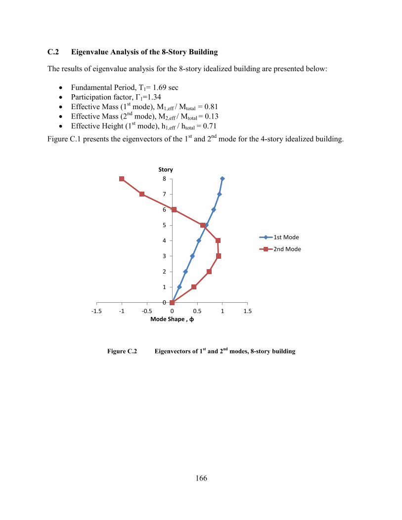
166






Effective Mass (2nd



Figure C.1 presents the eigenvectors of the 1st and 2

nd mode for the 4-story idealized building.



0

1

2

3

4

5

6

7

8

-1.5 -1 -0.5 0 0.5 1 1.5

Story

Mode Shape , φ

1st Mode

2nd Mode

167






Effective Mass (2nd





0

1

2

3

4

5

6

7

8

9

10

11

12

-1.5 -1 -0.5 0 0.5 1 1.5

Story

Mode Shape, φ

1st Mode

2nd Mode

168

D. An Approximate Procedure to Estimate the Base

Shear Capacity of Concrete Frame Buildings

The approximate procedure to estimate the base shear capacity of concrete frame buildings was

developed by Dr. M. Mehrain as part of the ATC-78 project (2013, 2014). A simplified version

of the suggested procedure is presented below.

In this method, the first step corresponds to estimation of the shear capacity of each story of the

studied building. Consequently the story capacities are used to estimate the base shear capacity.

The story shear capacity x is estimated as the sum of the individual column plastic capacities,

Vpcx at story x as shown in Equation D.1.

pcxpx VV (Eq. D.1)

where:

Vpcx is the lower between VpMx and Vnx, the column shear capacity controlled by flexure and shear

respectively. In the calculation of these strengths the axial load should be assumed equal to the

load according to approximate gravity analysis.

Vnx is the shear capacity of a column controlled by shear calculated according to Equation 4.1.

Vpmx is the plastic capacity of a column at story x calculated according to Equation D.2

x

cBxcTx

pMxh

MMV

(Eq. D.2)

169

McTx is calculated as the minimum of the flexural strength of the top of the column at story x or

the flexural strength at the top of the column controlled by the beams as defined in Equation D.3.

1

)1()1( *][

xx

xxbRxbL

cTxhh

hMMM (Eq. D.3)

Similarly McBx is calculated as the minimum of the flexural strength of the bottom of the column

at story x or the flexural strength at the bottom of the column controlled by the beams as defined

in Equation D.4.

1

*][

xx

xbRxbLx

cBxhh

hMMM (Eq. D.4)

Figure D.1 Schematic Drawing for the calculation of story plastic shear capacity

170

Calculation of VpM1 (1st Story Shear Capacity)

To account for the effect of boundary conditions located at the first story the method considers

two main cases:

a) Fixed Columns at Base: In that case calculation of top and bottom column strength

should be done according to the procedure described above, though h1 employed in

Equations D.2-4 should be assumed to be equal to 0.8 times the story height

(h1=0.8hstory).

b) Pinned Columns at Base: In that case calculation of top and bottom column strength

should be done according to the procedure described above, though h1 employed in

Equations D.2-4 should be assumed to be equal to 2.0 times the height of the story (2h).

Consequently, the shear demand on a structure at each story is computed based on an inverted

triangular load pattern. The story Demand over Capacity Ratio (DCR) is defined as the shear

demand for a specific story over the story shear capacity ,Vpx, calculated according to Equation

D.1.

The load pattern is increased by a constant factor for all stories over the height of the building

until the amplified shear demand hits the capacity curve at one or more stories (DCR=1.0) for

first time. The base shear of the building corresponding to this shear demand is taken as the

estimated maximum base shear capacity of the building Vmax,estimated.

Tables D.1-3 compare the base shear capacity estimated by Pushover Analysis and the

approximate method presented in this chapter. The difference in estimation of base shear

capacity between the two methods (pushover analysis and approximate method) ranges between

1% to 15%. The main reason for this difference is coming from the numerous assumptions that

the approximate method involves as well for the fact that the approximate method does not

account for the P-Delta effects.

In conclusion both pushover analysis and the approximate method could be utilized to estimate

the base shear capacity of concrete frame buildings. Depending on the method used to estimate

the base shear capacity two normalization factors are suggested for collapse risk evaluation:

a) Using Pushover Analysis, the Re factor as computed in Equation 5.1 should be used to

estimate the collapse performance of the studied building.

b) Using the Approximate Method to estimate the base shear capacity, the M factor as

computed in Equation 5.2 should be used to estimate the collapse performance of the

studied building.

The interested reader can find a more detailed description of the approximate method to estimate

the base shear capacity of concrete frame buildings in the ATC 78-1 and ATC 78-2 project

reports (2013, 2014).

171


4-story building

4-Story Building

ΣΜnc/ΣMnb Vmax,Pushover

(kips) Vmax,Estimated

(kips)

0.6 269.29 314.12

0.8 269.29 314.12

1 269.02 314.12

1.2 244.01 289.83

1.4 217.44 272.48

1.6 194.73 252.73

1.8 175.12 224.63


8-story Building

8-Story Building



(kips)

0.6 407.76 468.25

0.8 407.76 468.25

1 407.60 468.25

1.2 381.77 433.51

1.4 339.34 396.87

1.6 303.89 347.36

1.8 273.82 307.88

172


12-story building

12-Story Building



(kips)

0.6 591.39 686.79

0.8 591.39 686.79

1 589.67 686.79

1.2 574.00 613.8

1.4 506.31 525.92

1.6 453.41 460.77

1.8 407.77 409.41

173

E. Collapse Performance Tables for the Idealized

Buildings

In the current section, the collapse matrices that could be used to evaluate the collapse risk

according to the procedure described in Chapter 5 are presented. The collapse matrices are using

both the Re and M normalization factors to link structural parameters with probability of collapse

for the studied buildings.

Linear interpolation is suggested for the case of evaluating a building possessing intermediate

values for the studied structural parameters (building height, Vp/Vn, ΣMnc/ΣMnb)

E.1. 4-STORY BUILDING , COLLAPSE MATRICES USING THE RE FACTOR


(Re normalization factor)

Re ΣΜnc/ΣΜnb

2 3 4 5 6

0.6 0.02 0.18 0.44 0.68 0.83

0.8 0.02 0.19 0.45 0.68 0.83

1.0 0.02 0.15 0.39 0.62 0.79

1.2 0.00 0.06 0.19 0.36 0.54

1.4 0.00 0.03 0.11 0.24 0.37

1.6 0.00 0.01 0.04 0.12 0.25

1.8 0.00 0.01 0.03 0.10 0.19

174



Re ΣΜnc/ΣΜnb

2 3 4 5 6

0.6 0.08 0.40 0.70 0.88 0.95

0.8 0.09 0.40 0.71 0.88 0.95

1.0 0.08 0.40 0.70 0.88 0.95

1.2 0.03 0.21 0.47 0.69 0.83

1.4 0.02 0.10 0.26 0.44 0.60

1.6 0.01 0.05 0.15 0.29 0.44

1.8 0.00 0.02 0.08 0.17 0.29



Re ΣΜnc/ΣΜnb

2 3 4 5 6

0.6 0.18 0.58 0.84 0.95 0.98

0.8 0.17 0.58 0.84 0.95 0.98

1.0 0.16 0.54 0.81 0.93 0.98

1.2 0.05 0.31 0.61 0.81 0.92

1.4 0.02 0.16 0.38 0.59 0.75

1.6 0.01 0.08 0.22 0.38 0.54

1.8 0.00 0.03 0.11 0.24 0.39



Re ΣΜnc/ΣΜnb

2 3 4 5 6

0.6 0.68 0.82 0.94 0.98 1.00

0.8 0.68 0.83 0.94 0.98 1.00

1.0 0.67 0.81 0.93 0.97 1.00

1.2 0.23 0.55 0.80 0.90 0.99

1.4 0.03 0.22 0.52 0.75 0.89

1.6 0.01 0.11 0.30 0.51 0.68

1.8 0.01 0.06 0.19 0.35 0.50

175




Re ΣΜnc/ΣΜnb

2 3 4 5 6

0.6 0.10 0.43 0.73 0.89 0.96

0.8 0.10 0.44 0.74 0.89 0.96

1.0 0.09 0.37 0.65 0.82 0.92

1.2 0.02 0.14 0.35 0.56 0.72

1.4 0.00 0.03 0.14 0.32 0.50

1.6 0.00 0.01 0.08 0.21 0.37

1.8 0.00 0.01 0.06 0.15 0.29



Re ΣΜnc/ΣΜnb

2 3 4 5 6

0.6 0.31 0.68 0.88 0.95 0.98

0.8 0.33 0.69 0.88 0.96 0.98

1.0 0.31 0.67 0.86 0.95 0.98

1.2 0.08 0.33 0.58 0.76 0.87

1.4 0.02 0.13 0.34 0.55 0.72

1.6 0.00 0.06 0.20 0.38 0.56

1.8 0.00 0.03 0.13 0.28 0.44

176



Re ΣΜnc/ΣΜnb

2 3 4 5 6

0.6 0.46 0.83 0.95 0.99 1.00

0.8 0.45 0.82 0.95 0.99 1.00

1.0 0.41 0.78 0.93 0.98 0.99

1.2 0.13 0.44 0.70 0.86 0.93

1.4 0.03 0.21 0.47 0.68 0.82

1.6 0.02 0.12 0.32 0.52 0.69

1.8 0.00 0.06 0.20 0.39 0.57



Re ΣΜnc/ΣΜnb

2 3 4 5 6

0.6 0.70 0.93 0.99 1.00 1.00

0.8 0.67 0.92 0.98 0.99 1.00

1.0 0.65 0.93 0.99 1.00 1.00

1.2 0.23 0.64 0.87 0.96 0.99

1.4 0.10 0.37 0.62 0.79 0.89

1.6 0.02 0.16 0.40 0.62 0.78

1.8 0.01 0.09 0.27 0.49 0.67

177




Re ΣΜnc/ΣΜnb

2 3 4 5 6

0.6 0.12 0.55 0.85 0.96 0.99

0.8 0.12 0.54 0.85 0.96 0.99

1.0 0.08 0.45 0.79 0.93 0.98

1.2 0.03 0.24 0.56 0.79 0.91

1.4 0.00 0.08 0.30 0.55 0.75

1.6 0.00 0.04 0.18 0.40 0.62

1.8 0.00 0.03 0.14 0.32 0.52





Re ΣΜnc/ΣΜnb

2 3 4 5 6

0.6 0.65 0.93 0.99 1.00 1.00

0.8 0.65 0.93 0.99 1.00 1.00

1.0 0.56 0.91 0.99 1.00 1.00

1.2 0.16 0.60 0.87 0.96 0.99

1.4 0.05 0.33 0.65 0.85 0.94

1.6 0.01 0.17 0.46 0.72 0.87

1.8 0.01 0.11 0.35 0.61 0.79

Re ΣΜnc/ΣΜnb

2 3 4 5 6

0.6 0.52 0.89 0.98 1.00 1.00

0.8 0.52 0.89 0.98 1.00 1.00

1.0 0.44 0.85 0.97 0.99 1.00

1.2 0.09 0.44 0.75 0.91 0.97

1.4 0.02 0.18 0.48 0.73 0.87

1.6 0.00 0.09 0.32 0.58 0.78

1.8 0.00 0.06 0.23 0.46 0.66

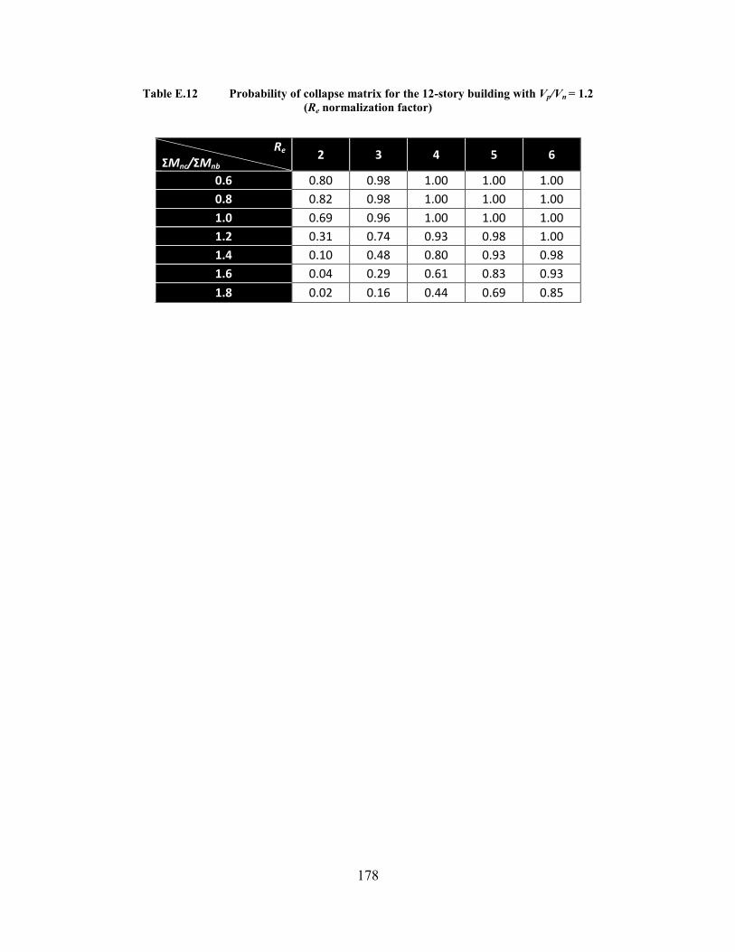
178



Re ΣΜnc/ΣΜnb

2 3 4 5 6

0.6 0.80 0.98 1.00 1.00 1.00

0.8 0.82 0.98 1.00 1.00 1.00

1.0 0.69 0.96 1.00 1.00 1.00

1.2 0.31 0.74 0.93 0.98 1.00

1.4 0.10 0.48 0.80 0.93 0.98

1.6 0.04 0.29 0.61 0.83 0.93

1.8 0.02 0.16 0.44 0.69 0.85

179

E.4. 4-STORY BUILDING , COLLAPSE MATRICES USING THE M FACTOR


(M normalization factor)

M ΣΜnc/ΣΜnb

2 3 4 5 6

0.6 0.03 0.20 0.46 0.69 0.84

0.8 0.03 0.20 0.46 0.69 0.84

1.0 0.02 0.16 0.41 0.64 0.80

1.2 0.01 0.07 0.21 0.39 0.57

1.4 0.01 0.05 0.15 0.30 0.45

1.6 0.00 0.02 0.08 0.20 0.35

1.8 0.00 0.01 0.06 0.15 0.27



M ΣΜnc/ΣΜnb

2 3 4 5 6

0.6 0.17 0.58 0.85 0.95 0.99

0.8 0.17 0.57 0.84 0.94 0.98

1.0 0.17 0.57 0.83 0.94 0.98

1.2 0.08 0.36 0.64 0.83 0.92

1.4 0.05 0.22 0.45 0.64 0.78

1.6 0.03 0.14 0.32 0.50 0.65

1.8 0.01 0.06 0.19 0.35 0.50

180



M ΣΜnc/ΣΜnb

2 3 4 5 6

0.6 0.31 0.74 0.92 0.98 0.99

0.8 0.31 0.74 0.92 0.98 0.99

1.0 0.28 0.70 0.91 0.97 0.99

1.2 0.13 0.49 0.77 0.91 0.97

1.4 0.08 0.32 0.59 0.78 0.89

1.6 0.04 0.20 0.41 0.60 0.73

1.8 0.01 0.10 0.26 0.45 0.57



M ΣΜnc/ΣΜnb

2 3 4 5 6

0.6 0.71 0.97 0.99 1.00 1.00

0.8 0.71 0.97 0.99 1.00 1.00

1.0 0.66 0.90 0.99 1.00 1.00

1.2 0.31 0.68 0.85 0.92 0.97

1.4 0.10 0.40 0.65 0.82 0.90

1.6 0.02 0.18 0.44 0.67 0.80

1.8 0.01 0.10 0.30 0.52 0.69




M ΣΜnc/ΣΜnb

2 3 4 5 6

0.6 0.19 0.59 0.84 0.95 0.98

0.8 0.19 0.59 0.84 0.95 0.98

1.0 0.16 0.51 0.77 0.90 0.96

1.2 0.04 0.22 0.47 0.68 0.81

1.4 0.01 0.08 0.26 0.48 0.66

1.6 0.00 0.03 0.14 0.33 0.52

1.8 0.00 0.02 0.10 0.23 0.40

181



M ΣΜnc/ΣΜnb

2 3 4 5 6

0.6 0.47 0.81 0.94 0.98 0.99

0.8 0.47 0.81 0.94 0.98 0.99

1.0 0.46 0.80 0.93 0.98 0.99

1.2 0.16 0.47 0.72 0.86 0.94

1.4 0.05 0.26 0.52 0.72 0.85

1.6 0.04 0.17 0.33 0.55 0.72

1.8 0.01 0.07 0.22 0.41 0.58



M ΣΜnc/ΣΜnb

2 3 4 5 6

0.6 0.60 0.90 0.98 1.00 1.00

0.8 0.59 0.90 0.98 0.99 1.00

1.0 0.55 0.87 0.97 0.99 1.00

1.2 0.25 0.56 0.80 0.91 0.96

1.4 0.12 0.38 0.62 0.81 0.91

1.6 0.05 0.24 0.44 0.65 0.80

1.8 0.02 0.14 0.29 0.51 0.68



M ΣΜnc/ΣΜnb

2 3 4 5 6

0.6 0.74 0.94 0.99 1.00 1.00

0.8 0.74 0.94 0.99 1.00 1.00

1.0 0.74 0.94 0.99 1.00 1.00

1.2 0.30 0.71 0.91 0.97 0.99

1.4 0.16 0.46 0.71 0.86 0.93

1.6 0.04 0.22 0.49 0.70 0.84

1.8 0.01 0.12 0.33 0.56 0.73

182




M ΣΜnc/ΣΜnb

2 3 4 5 6

0.6 0.43 0.87 0.98 1.00 1.00

0.8 0.43 0.86 0.98 1.00 1.00

1.0 0.34 0.81 0.96 0.99 1.00

1.2 0.09 0.38 0.65 0.85 0.92

1.4 0.00 0.15 0.40 0.65 0.80

1.6 0.00 0.10 0.25 0.48 0.65

1.8 0.00 0.08 0.20 0.35 0.55





M ΣΜnc/ΣΜnb

2 3 4 5 6

0.6 0.79 0.97 1.00 1.00 1.00

0.8 0.79 0.97 1.00 1.00 1.00

1.0 0.72 0.96 1.00 1.00 1.00

1.2 0.30 0.69 0.91 0.98 1.00

1.4 0.15 0.42 0.69 0.88 0.95

1.6 0.10 0.28 0.48 0.73 0.88

1.8 0.05 0.17 0.35 0.61 0.79

M ΣΜnc/ΣΜnb

2 3 4 5 6

0.6 0.69 0.95 0.99 1.00 1.00

0.8 0.69 0.95 0.99 1.00 1.00

1.0 0.62 0.93 0.99 1.00 1.00

1.2 0.14 0.53 0.82 0.94 0.98

1.4 0.02 0.21 0.52 0.76 0.89

1.6 0.01 0.10 0.34 0.60 0.79

1.8 0.00 0.06 0.23 0.46 0.66

183



M ΣΜnc/ΣΜnb

2 3 4 5 6

0.6 0.90 0.99 1.00 1.00 1.00

0.8 0.91 0.99 1.00 1.00 1.00

1.0 0.83 0.99 1.00 1.00 1.00

1.2 0.39 0.81 0.95 0.99 1.00

1.4 0.20 0.53 0.83 0.95 0.99

1.6 0.05 0.31 0.63 0.84 0.94

1.8 0.02 0.17 0.45 0.69 0.85

184

F. Approximate Relationships to Estimate the

Fundamental Building Period7

Goel and Chopra (1994) reported measured values of building period, T, for concrete frame

buildings as a function of building height only. In ASCE-41 these data have been conservatively

approximated (a shortened period results in greater base shear for most cases) by Equation F.1.

9.0

41 *018.0 HTASCE (Eq. F.1)

where, H corresponds to the building height in feet.

Equation F.1 corresponds to a simplified approach that does not consider explicitly other

building characteristics that are expected to influence significantly the fundamental building

period such as the member sizes, the steel reinforcement and the corresponding building

strength.

An alternative procedure was developed by Dr. Mehrain for the purposes of the ATC-78 model

(ATC-78, 2014), based on results obtained from pushover analysis. The suggested equation as

presented in ATC-78 report is shown below:

y

building

ATCV

WHT

**078.078 (Eq. F.2)

where, Hbuilding corresponds to the building height in feet, W is the building weight and Vy is the

base shear yielding strength (W and Vy should be given in the same units).

F.1. MATHEMATICAL MODEL TO DETERMINE THE FUNDAMENTAL

BUILDING PERIOD

Determination of the natural frequencies and modes of a structure, requires solution of the matrix

eigenvalue problem presented in Equation F.3

7 The contribution of Ms. Francesca Renouard in the development of Appendix G is acknowledged

185

(K-ωn2*M)*Φn=0 (Eq. F.3)

where, K corresponds to the building stiffness matrix, M corresponds to the building mass

matrix, ωn2 corresponds to the eigenvalues and Φn to the matrix of eigenvectors. Equation F.4

defines the natural frequency ωn of the building.

n

nω

2

(Eq. F.4)

where, Tn is the nth

-mode building period (T1 is the 1st mode or fundamental building period)

The eigenvalues ωn2

are the roots of Equation F.5.

det [K-ωn2*M] =0 (Eq. F.5)

F.2. USING SIMPLIFIED FISHBONE MODELS TO APPROXIMATE THE

FUNAMENTAL BUILDING PERIOD

Nakashima et al. (2002) and Luco et al. (2003) suggested a generic frame model (or otherwise

termed as “fishbone” model) as a computationally efficient alternative to predict the dynamic

response of moment frames rather than modeling the whole structure.

In the current study the generic frame as suggested by Nakashima was utilized to generate a

range of buildings with different structural properties such as flexural strength, reinforcement

ratio, column dimensions and building height.

An example of a generic frame model is shown in Figure F.1. The generic frame model lumps

column and beam stiffnesses by condensing all the columns of a story into one column and

condensing all the beams into two beams with length equal to the length of the mid-span of a

typical bay corresponding to the studied frame.

186

Figure F.1 Schematic illustration of the generic frame model (on the right) used to represent

the idealized 8-story building (on the left)

The following structural parameters were used as an input to design generic frame models

equivalent to the corresponding concrete moment frames with the assumed building

characteristics.

Building height, H

Base shear strength normalized by the building weight, V/W

Average column longitudinal reinforcement ratio, long

For the generic frames designed, it was assumed that the equivalent structural moment frames

consist of five bays, with dimensions, material properties and gravity loading per floor equal to

the values used for the idealized building presented in Appendix A. All the beam members were

assumed to possess longitudinal reinforcement ratio equal to 0.01.

To design the generic frames, an inverted lateral triangular load pattern was considered; the

gravity forces were assumed to be the same with those used for the design of the idealized

buildings (see Appendix A). The flexural forces determined from the generic frame analytical

model were reduced by the factor, Z, provided in Equations F.6-1-3 to estimate the equivalent

frame individual member forces.

Mcolumn,frame=Zcolumn*M G.F.,column (Eq. F.6-1)

187

Mbeam,frame=Zbeam*M G.F.,beam (Eq. F.6-2)

Z=

(Eq. F.6-3)

where, Njoints corresponds to the total number of beam-column joints per story of interest,

MG.F.,column is the bending moment at the top or bottom of the column members of the generic

frame model, and MG.F.,beam is the bending moment at the beam joint of the generic frame.

The column and beam reinforcement ratio were set constant and the member dimensions were

estimated such that Equation F.7 (Panagiotakos, 2001), is satisfied:

{

( ( )

)

[( ) ( )

( )] ( )}

(Eq. F.7)

where,

( ) (Eq. F.7-1)

My = member yield moment (kip-in)

fy = yield strength of reinforcement steel (ksi)

Es = modulus of elasticity of reinforcement steel (ksi)

Ec = modulus of elasticity of concrete (ksi)

d = effective depth of cross section (in)

d’ = distance of center of compression reinforcement from extreme compression fiber (in)

( ) (Eq. F.7-2)

(Eq. F.7-3)

( ) (Eq. F.7-4)

ρ = tension reinforcement ratio

ρ’ = compression reinforcement ratio

ρv = reinforcement ratio of transverse steel

N = axial force (kip)

δ' = d’/d (Eq. F.7-5)

The following constraints were used to better emulate actual construction and member size

selection:

188

Column and beam sizes were changed every two stories.

Column size was limited to no smaller than 12” x 12”.

Beam depth to width ratio limited to no greater than 1.5.

After the member dimensions have been determined such that they satisfy certain flexural

strength demands and reinforcement properties, the effective moment of inertia was calculated

according to the procedure suggested by Elwood and Eberhard (2006) as follows:

y

y

calcff

LMI

*6

*=E

2

,e (Eq. F.8)

Where My is calculated according to Equation F.7, Δy is calculated according to Equation F.8-1

and L is the corresponding column height

Δy=Δflex+Δslip 8 (Eq. F.8-1)

where,

Δflex corresponds to the displacement due to flexural deformations

y

L

6=Δ

2

flex (Eq. F.8-2)

Δslip corresponds to the displacement due to bar slip

u

fLd ysb

8=Δslip

(Eq. F.8-3)

L=column height (in)

φy=yield curvature

fs=stress of tensions reinforcement (psi)

db=diameter of longitudinal reinforcement (in)

u=average bond stress assumed to be equal cf '6 (psi)

Using the generic frame geometry and the effective stiffness properties as calculated according

to Equation F.8-1-3 eigenvalue analysis was performed using OpenSees structural analysis

software.

Applying the geometric and reinforcement properties of the idealized 4, 8 and 12 story buildings

used in the current study (Appendix A) eigenvalue analysis was performed to test the accuracy of

8 The deformation due to shear was not included, assuming to be negligible for the elastic deformation range

189

the generic frame model in predicting the dynamic response of frame buildings. Table F.1

compares the results of the fundamental period obtained from eigenvalue analysis of the

idealized buildings and the equivalent generic frames.

Table F.1 Comparison of eigenvalue analysis of the idealized building models and the equivalent

generic frame model

Period (sec)

Building Idealized Building

Generic Frame

4-Story 1.14 1.11

8-Story 1.62 1.52

12-Story 1.95 1.81

The results demonstrate that the generic frame model provides good accuracy in estimation of

the actual building period of the idealized buildings.

F.3. EFFECT OF STRUCTURAL PARAMETERS AND BUILDING GEOMETRY IN

ESTIMATION OF THE FUNDAMENTAL BUILDING PERIOD

The following structural parameters were used to produce building variations as generic frame

models equivalent to concrete moment frames possessing similar structural properties.

Building height, H (ft): 46 ft (4-story bldg..) , 90 ft (8-story bldg..) , 134 ft (12-story

bldg..)

Base shear strength normalized by the building weight, V9/W: 0.05 , 0.10, 0.15, 0.25.

Average column longitudinal reinforcement ratio, long :0.01, 0.015, 0.018,0.02, 0.025,

and 0.03

Figures F.2 –F.4 show how the structural parameters discussed above influence the fundamental

period of the building.

9 V can be estimated by ΣVpM1 (sum of the flexural column strength of the 1

st story) as defined in Appendix E

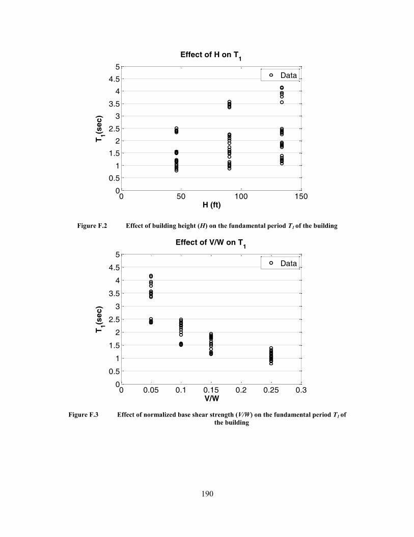
190

Figure F.2 Effect of building height (H) on the fundamental period T1 of the building

Figure F.3 Effect of normalized base shear strength (V/W) on the fundamental period T1 of

the building

0 50 100 1500

0.5

1

1.5

2

2.5

3

3.5

4

4.5

5

H (ft)

T1(s

ec

)

Effect of H on T1

Data

0 0.05 0.1 0.15 0.2 0.25 0.30

0.5

1

1.5

2

2.5

3

3.5

4

4.5

5

V/W

T1(s

ec

)

Effect of V/W on T1

Data

191

Figure F.4 Effect of longitudinal reinforcement ratio (ρlong) on the fundamental period T1 of

the building

As illustrated in Figure F.2, building height is significantly influencing the fundamental period of

the building. Increasing building height results in higher fundamental period values. However in

the same Figure we observe large dispersion for all the studied building heights. The main reason

for this is the different V/W ratio values that the building is designed for. Contrary to Equation

F.1 which suggests that the building height is the only parameter that affects the building

fundamental period, the normalized base shear strength (V/W) according to Figure F.3 also

influences greatly the fundamental period. On the other hand, the column longitudinal

reinforcement ratio does not seem to dramatically influence the fundamental building period.

Figure F.4 demonstrates that as ρlong increases, T1 tends to increase as well, but less pronounced

in comparison with the other two considered parameters, H and V/W.

Using the observed data from the building variations discussed above an analytical model to

estimate the building period should be defined according to the following form:

),/,(1.,. longFG WVHfT (Eq. F.8)

Based on the aforementioned model, forward stepwise linear regression of the form shown in

Equation F.9 was used:

)ln(*)/ln()ln()ln( 32101.,. longFG WVHT (Eq. F.9)

0 0.01 0.02 0.03 0.040

0.5

1

1.5

2

2.5

3

3.5

4

4.5

5

long

T1(s

ec

)

Effect of long

on T1

Data

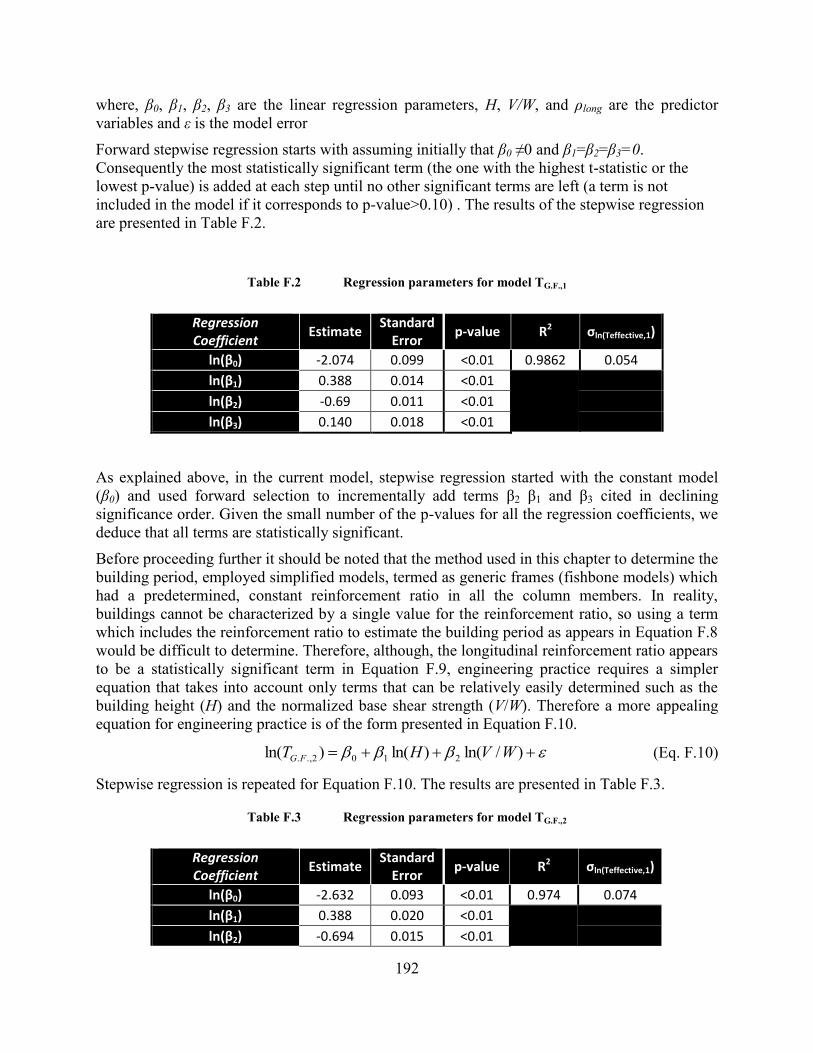
192

where, β0, β1, β2, β3 are the linear regression parameters, H, V/W, and ρlong are the predictor

variables and ε is the model error

Forward stepwise regression starts with assuming initially that β0 ≠0 and β1=β2=β3=0.

Consequently the most statistically significant term (the one with the highest t-statistic or the

lowest p-value) is added at each step until no other significant terms are left (a term is not

included in the model if it corresponds to p-value>0.10) . The results of the stepwise regression

are presented in Table F.2.

Table F.2 Regression parameters for model TG.F.,1

Regression Coefficient

Estimate Standard

Error p-value R2 σln(Teffective,1)

ln(β0) -2.074 0.099 <0.01 0.9862 0.054

ln(β1) 0.388 0.014 <0.01

ln(β2) -0.69 0.011 <0.01

ln(β3) 0.140 0.018 <0.01

As explained above, in the current model, stepwise regression started with the constant model

(β0) and used forward selection to incrementally add terms β2 β1 and β3 cited in declining

significance order. Given the small number of the p-values for all the regression coefficients, we

deduce that all terms are statistically significant.

Before proceeding further it should be noted that the method used in this chapter to determine the

building period, employed simplified models, termed as generic frames (fishbone models) which

had a predetermined, constant reinforcement ratio in all the column members. In reality,

buildings cannot be characterized by a single value for the reinforcement ratio, so using a term

which includes the reinforcement ratio to estimate the building period as appears in Equation F.8

would be difficult to determine. Therefore, although, the longitudinal reinforcement ratio appears

to be a statistically significant term in Equation F.9, engineering practice requires a simpler

equation that takes into account only terms that can be relatively easily determined such as the

building height (H) and the normalized base shear strength (V/W). Therefore a more appealing

equation for engineering practice is of the form presented in Equation F.10.

)/ln()ln()ln( 2102.,. WVHT FG (Eq. F.10)

Stepwise regression is repeated for Equation F.10. The results are presented in Table F.3.

Table F.3 Regression parameters for model TG.F.,2

Regression Coefficient

Estimate Standard

Error p-value R2 σln(Teffective,1)

ln(β0) -2.632 0.093 <0.01 0.974 0.074

ln(β1) 0.388 0.020 <0.01

ln(β2) -0.694 0.015 <0.01

193

As expected, the simplified model of Equation F.10 gives higher value for the standard deviation

of the model error compared to Equation F.9 that includes also the ρlong parameter. The increase

in the standard deviation though is judged not to be so important for structural engineering

purposes taking into account the difficulty that it would entail defining a unique value for ρlong

for an real building.

Substituting the regression coefficient values corresponding to linear regression, Equation F.10

can be written as follows:

69.039.0

2,. )/(**072.0 WVHT FG (Eq. F.11)

Figure F.5 provides a comparison of the relationships for estimation of the building period.


Looking at the graphs in Figure F.5 the following observations can be made:

Increasing the building height for the same normalized base shear strength corresponds to

higher building period values

0.05 0.1 0.15 0.2 0.250

0.5

1

1.5

2

2.5

3

V/W

T1(s

ec)

4-Story Building

TG.F.1

=0.126 *(V/W)(-0.69)

*H0.39

*(long

=0.005)0.14

TG.F.1

=0.126 *(V/W)(-0.69)

*H0.39

*(long

=0.010)0.14

TG.F.1

=0.126 *(V/W)(-0.69)

*H0.39

*(long

=0.015)0.14

TG.F.1

=0.126 *(V/W)(-0.69)

*H0.39

*(long

=0.020)0.14

TG.F.1

=0.126 *(V/W)(-0.69)

*H0.39

*(long

=0.025)0.14

TG.F.2

=0.072 *(V/W)(-0.69)

*H0.39

TATC-78

=0.078 *(V/W)-0.50

*H0.5

TASCE41

=0.018 *H0.90

0.05 0.1 0.15 0.2 0.250

0.5

1

1.5

2

2.5

3

3.5

4

V/W

T1(s

ec)

8-Story Building

0.05 0.1 0.15 0.2 0.250

0.5

1

1.5

2

2.5

3

3.5

4

V/W

T1(s

ec)

12-Story Building

194

Increasing the normalized base shear strength for the same height corresponds to a

decrease in the building period values.

Increasing the longitudinal reinforcement ratio for the same normalized base shear

strength and height results in an increase in the fundamental building period since it

corresponds to smaller member sizes.

Equation F.11 estimates with sufficient accuracy for structural engineering applications

the fundamental building period. Given the fact that Equation F.9 involves an additional

term (ρlong) that it is hard to be defined with a single value for a real building, Equation

F.11 seems to provide an appealing alternative for estimating the building period.

The trends discussed above are in agreement with physical intuition and with physical data

provided in the literature.

A comparison of relationships provided by Equations F.1, F.2 and F.11 with the analytical data

obtained from eigenvalue analysis using simplified generic frame models are presented in

Figures F.6 and F.7. Equations F.2 and F.11 seem to provide relatively accurate estimates of the

effective period obtained from analytical results, while the Equation suggested by ASCE-41

provides systematically lower estimates of the fundamental building period for buildings with

normalized base shear strength V/W<0.20.

195


with analytical data (Effect of V/W on T1)

0.05 0.1 0.15 0.2 0.250

0.5

1

1.5

2

2.5

3

V/W

T1(s

ec)

4-Story Building

Data

TG.F.2

=0.072 *(V/W)(-0.69)

*H0.39

TATC-78

=0.078 *(V/W)-0.50

*H0.50

TASCE41

=0.018 *H0.19

0.05 0.1 0.15 0.2 0.250

0.5

1

1.5

2

2.5

3

3.5

4

V/W

T1(s

ec)

8-Story Building

0.05 0.1 0.15 0.2 0.250

0.5

1

1.5

2

2.5

3

3.5

4

V/W

T1(s

ec)

12-Story Building

196


with analytical data (Effect of H on T1)

As shown in Table F.4 the data from the Equations F.2 and F.11 provide good approximations of

the periods of the idealized buildings used in this study obtained from eigenvalue analysis.

Table F.4 Comparison of eigenvalue analysis of the idealized building models and the estimated

building period values

Period (sec)

Idealized Building Eigenvalue

Analysis TG.F.,2 TATC-78 TASCE-41

4-Story 1.14 0.96 1.16 0.57

8-Story 1.62 1.51 1.87 1.03

12-Story 1.95 1.81 2.33 1.48

0 50 100 1500

0.5

1

1.5

2

2.5

3

3.5

4

4.5

5

H (ft)

T1(s

ec)

V/W=0.05

Data

TG.F.2

=0.072 *(V/W)(-0.69)

*H0.39

TATC-78

=0.078 *(V/W)-0.50

*H0.50

TASCE41

=0.018 *H0.90

0 50 100 1500

0.5

1

1.5

2

2.5

3

3.5

4

4.5

5

H (ft)

T1(s

ec)

V/W=0.10

0 50 100 1500

0.5

1

1.5

2

2.5

3

3.5

4

4.5

5

H (ft)

T1(s

ec)

V/W=0.15

197

In conclusion, Equation F.11 seems to provide overall the best estimates of the building period

for the concrete frame buildings analyzed in the current study. Equation F.2 provides also a good

approximation of the analytical results. Therefore, for the purposes of the current study T1

(fundamental building period) will be approximated with TG.F. as shown in equation F.12:

69.039.0

. )/(**072.0 WVHT FG (Eq. F.12)

198

G. Story Drift Profiles

Equation 6.4 provided in Chapter 6 relates the maximum10 story drift ratio demand with the

estimated average drift ratio observed in the studied building.

As discussed in Chapter 2, Shome and Cornell (1999), used statistical regression for numerous

non-linear dynamic analyses to estimate story drift ratios. Shome and Cornell employed

different predictors to estimate the story drift ratio. The predictors included Spectral acceleration

at the building 1st mode period (Sa(T1) ), Spectral acceleration at the 2

nd mode period (Sa(T2) ),

earthquake magnitude (M) , epicentral distance (R), and ground motion duration (D). The

statistical processing of the results showed that the spectral acceleration at the 1st mode period

constitutes the most statistically significant parameter, while for taller buildings the spectral

acceleration at the 2nd

mode period influences also the predicted variable. The results of Shome’s

study indicated that story drift ratio demand is almost a linear function of Sa(T1).

Using the results of IDA, this study initially related the story drift ratio demand with Sa(T1)

using a similar statistical model with the one suggested by Shome and Cornell, presented in

Equation G.1

)))(((

ln(*)ln(1

10

eff

eff

x

x

h

TSaf

h (Eq. G.1)

where, δx is the story drift demand, , hx is the story height, αx is the coefficient for story x used to

estimate the story drift pattern, δeff is the displacement at the effective floor height calculated

according to Equation 6.1 (δeff is a function of Sa(T1), heff is the story height (assumed to be

heff=0.7*hbuilding,, where hbuidling is the total building height)

The results of statistical regression using Equation G.1 confirmed the findings of Shome’s study:

The estimated values of coefficient β1 ranged from 0.93 to 1.07. Based on this we could

assume that the story drift ratio demand is approximately a linear function of δeff (δeff

employed in Equation G.1 was calculated according to Equation 6.1, where δeff is a

function of Sa(T1)) , and thus of Sa(T1) .

10

The term maximum corresponds to the maximum value of drift ratio expected over the entire dynamic response of

the building for each story. For brevity the word maximum will be omitted when the term story drift ratio demand is

used.

199

For buildings possessing strong columns –weak beams (ΣΜnc/ΣΜnb ≥1.20) , β0 was

estimated approximately equal to 1.5, in agreement with the value suggested by Shome

and Cornell using 5 and 20-story moment resisting frames (see Chapter 2).

Although a more complicated statistical model could be utilized to relate (δx/hx) with (δeff/heff), a

linear model with a single coefficient, β0=ln(αx) (β1 was set equal to unity based on the findings

mentioned above), was employed . This allows an engineer to directly observe and understand

the effect of each structural parameter to the drift pattern of the building. To calibrate the

coefficient β0=ln(αx) for each story of the studied building, a linear model with the form shown

in Equation G.2 was fitted such that the sum of the squares of the errors in the analyzed model is

minimized.

)ln()ln()ln(eff

eff

x

x

x

ha

h (Eq. G.2)

The data used for fitting equation G.2 were taken from numerous non-linear dynamic analysis

that were performed as part of IDA employing ground motions with scaling factor values slightly

lower than those leading to building collapse.

It should be noted that Equation G.2 was suggested to fit the data by practicing engineers due to

its simplicity and engineering appeal. The goodness of fit of the model presented in Equation G.2

was checked visually.

In the current study it was preferred to perform separate statistical regression for different

ΣΜnc/ΣΜnb and Vp/Vn building variations such that the estimates of ln(αx) could be defined

according to statistics but also engineering judgment.

However, an alternative approach could also be followed employing both ΣΜnc/ΣΜnb ratio and

Vp/Vn ratio as predictors. The alternative statistical model is shown in Equation G.3:

npnbnc

eff

eff

x

x VVMhh

/*/*)ln(*)ln( 3210 (Eq. G.3)

Although Equation G.3 seemed to estimate more accurately the story drift ratio demand, it was

recognized that in reality it would be rare to find buildings with column members possessing

uniform values of ΣΜnc/ΣΜnb and Vp/Vn in a specific story. Thus, Equation G.2 was preferred

for the estimation of story drift ratio demand. due to its simplicity.

Due to the lack of sufficient amount of studies, confirming the relationship between story drift

ratio demand and average drift ratio, the values of ln(αx) in this study were selected such that the

estimate of the story drift ratio demand would be more conservative than what statistical

regression of the Equation G.2 would provide for the weaker/critical story.

Figure G.1 compares the results obtained from Equation G.2 with analytical data obtained from

IDA for the critical 1st story. As we observe in Figure G.1, for a certain value of average drift

ratio (δeff/heff) there is large variability in the 1st story drift ratio demand(δ1/h1) (typical values of

the coefficient of determination, R2,

of the model presented in Equation G.2 range from 0.35 to

0.70 for the critical story regression estimates).

200

This indicates that further research is required in the future to select a more accurate statistical

model to relate story drift ratio demand with estimated building displacements such that an

optimal balance of goodness of fit and simplicity can be obtained.

Figure G.1 Observed story drift ratio demand (δ1/h1) at the 1st story over estimated average

drift (δeff/heff) (8-Story building, Vp/Vn=0.8, ΣΜnc/ΣΜnb=1.20)

Tables G.1-G.3 present the estimated values of αx=exp( 0 ) and the standard deviation of the

natural logarithm of the story drift ratio demand based on statistical regression for different

variations of the idealized 4,8 and 12-story buildings.

0 0.01 0.02 0.030

0.01

0.02

0.03

eff

/heff

1/h

1

1/h

1=

1*

eff/h

eff

+/- std.

Analytical Data(IDA)

201


Vp/Vn=0.8

ΣΜnc/ΣΜnb

Story 0.6 0.8 1.0 1.2 1.4 1.6 1.8

4 0.53 0.53 0.53 0.49 0.48 0.53 0.61

3 0.90 0.90 0.88 0.83 0.85 0.92 0.99

2 0.84 0.84 0.87 1.00 1.12 1.21 1.25

1 1.93 1.93 1.90 1.68 1.48 1.33 1.22

Vp/Vn=1.0

ΣΜnc/ΣΜnb

Story 0.6 0.8 1.0 1.2 1.4 1.6 1.8

4 0.57 0.56 0.56 0.54 0.52 0.56 0.61

3 0.94 0.95 0.92 0.90 0.88 0.95 1.01

2 0.92 0.91 0.93 1.05 1.14 1.22 1.26

1 1.81 1.82 1.78 1.56 1.44 1.32 1.22

Vp/Vn=1.2

ΣΜnc/ΣΜnb

Story 0.6 0.8 1.0 1.2 1.4 1.6 1.8

4 0.58 0.58 0.58 0.55 0.56 0.55 0.61

3 0.90 0.90 0.91 0.90 0.93 0.95 1.03

2 1.00 1.00 1.01 1.09 1.17 1.22 1.27

1 1.68 1.68 1.64 1.51 1.39 1.29 1.20

)0ˆ( expxα

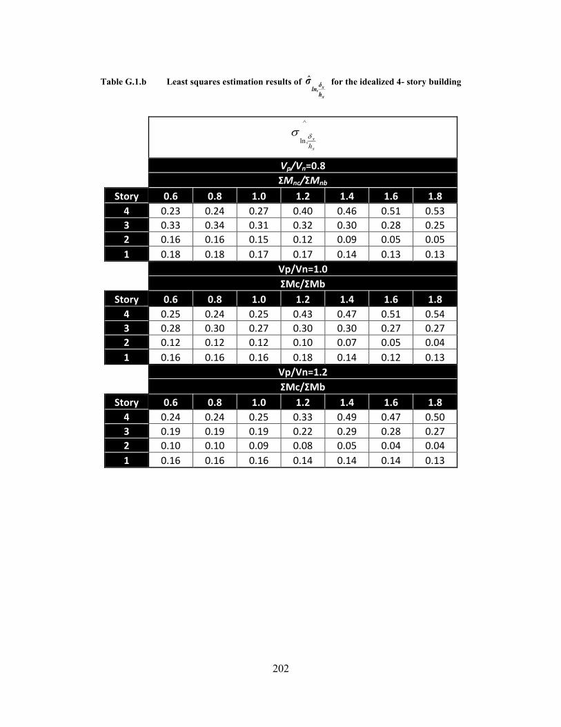
202


x

x

h

δln,


Vp/Vn=0.8

ΣΜnc/ΣΜnb

Story 0.6 0.8 1.0 1.2 1.4 1.6 1.8

4 0.23 0.24 0.27 0.40 0.46 0.51 0.53

3 0.33 0.34 0.31 0.32 0.30 0.28 0.25

2 0.16 0.16 0.15 0.12 0.09 0.05 0.05

1 0.18 0.18 0.17 0.17 0.14 0.13 0.13

Vp/Vn=1.0

ΣΜc/ΣΜb

Story 0.6 0.8 1.0 1.2 1.4 1.6 1.8

4 0.25 0.24 0.25 0.43 0.47 0.51 0.54

3 0.28 0.30 0.27 0.30 0.30 0.27 0.27

2 0.12 0.12 0.12 0.10 0.07 0.05 0.04

1 0.16 0.16 0.16 0.18 0.14 0.12 0.13

Vp/Vn=1.2

ΣΜc/ΣΜb

Story 0.6 0.8 1.0 1.2 1.4 1.6 1.8

4 0.24 0.24 0.25 0.33 0.49 0.47 0.50

3 0.19 0.19 0.19 0.22 0.29 0.28 0.27

2 0.10 0.10 0.09 0.08 0.05 0.04 0.04

1 0.16 0.16 0.16 0.14 0.14 0.14 0.13

^

ln,x

x

h

203


Vp/Vn=0.8

ΣΜnc/ΣΜnb

Story 0.6 0.8 1.0 1.2 1.4 1.6 1.8

8 1.01 1.01 0.91 0.84 0.65 0.59 0.63

7 1.50 1.50 1.43 1.30 1.08 0.95 0.95

6 1.60 1.60 1.60 1.50 1.28 1.18 1.17

5 1.63 1.62 1.54 1.38 1.24 1.21 1.27

4 0.93 0.93 0.91 1.03 1.09 1.18 1.28

3 1.12 1.12 1.05 1.14 1.31 1.37 1.45

2 0.89 0.89 0.88 1.21 1.40 1.41 1.42

1 1.96 1.96 1.92 1.63 1.46 1.32 1.21

Vp/Vn=1.0

ΣΜnc/ΣΜnb

Story 0.6 0.8 1.0 1.2 1.4 1.6 1.8

8 0.91 0.90 0.94 0.82 0.71 0.65 0.59

7 1.47 1.46 1.49 1.38 1.20 1.08 0.97

6 1.61 1.61 1.62 1.58 1.42 1.33 1.23

5 1.53 1.54 1.52 1.43 1.34 1.29 1.30

4 0.98 0.98 0.98 1.05 1.12 1.20 1.29

3 1.14 1.15 1.11 1.15 1.27 1.35 1.41

2 0.94 0.94 0.95 1.20 1.34 1.38 1.38

1 1.85 1.86 1.81 1.48 1.33 1.26 1.15

Vp/Vn=1.2

ΣΜnc/ΣΜnb

Story 0.6 0.8 1.0 1.2 1.4 1.6 1.8

8 0.95 0.97 0.96 0.88 0.79 0.68 0.66

7 1.52 1.53 1.52 1.46 1.35 1.18 1.08

6 1.69 1.67 1.69 1.66 1.56 1.44 1.30

5 1.55 1.54 1.52 1.49 1.40 1.36 1.31

4 1.06 1.05 1.05 1.10 1.13 1.21 1.27

3 1.17 1.17 1.16 1.15 1.25 1.34 1.41

2 1.05 1.04 1.05 1.19 1.30 1.36 1.38

1 1.69 1.68 1.68 1.38 1.25 1.19 1.14

)0ˆ( expxα

204


x

x

h

δln,


Vp/Vn=0.8

ΣΜnc/ΣΜnb

Story 0.6 0.8 1.0 1.2 1.4 1.6 1.8

8 0.46 0.47 0.46 0.52 0.45 0.48 0.46

7 0.46 0.46 0.45 0.43 0.45 0.47 0.43

6 0.30 0.30 0.32 0.33 0.38 0.40 0.35

5 0.32 0.31 0.28 0.28 0.30 0.28 0.23

4 0.19 0.20 0.18 0.20 0.20 0.15 0.14

3 0.29 0.29 0.27 0.20 0.16 0.14 0.14

2 0.24 0.24 0.24 0.20 0.23 0.22 0.22

1 0.31 0.30 0.32 0.35 0.31 0.30 0.30

Vp/Vn=1.0

ΣΜnc/ΣΜnb

Story 0.6 0.8 1.0 1.2 1.4 1.6 1.8

8 0.38 0.39 0.43 0.39 0.27 0.29 0.29

7 0.75 0.75 0.73 0.59 0.43 0.37 0.36

6 0.52 0.52 0.54 0.49 0.42 0.39 0.38

5 0.45 0.44 0.45 0.37 0.35 0.32 0.29

4 0.12 0.12 0.13 0.19 0.20 0.16 0.15

3 0.37 0.37 0.27 0.23 0.19 0.17 0.17

2 0.15 0.14 0.16 0.22 0.28 0.26 0.26

1 0.54 0.54 0.52 0.46 0.39 0.32 0.31

Vp/Vn=1.2

ΣΜnc/ΣΜnb

Story 0.6 0.8 1.0 1.2 1.4 1.6 1.8

8 0.41 0.42 0.42 0.45 0.52 0.45 0.46

7 0.42 0.43 0.41 0.41 0.47 0.44 0.41

6 0.31 0.30 0.30 0.32 0.38 0.36 0.33

5 0.23 0.23 0.22 0.23 0.27 0.26 0.25

4 0.12 0.13 0.13 0.18 0.20 0.17 0.15

3 0.22 0.23 0.21 0.19 0.18 0.17 0.16

2 0.19 0.20 0.20 0.19 0.24 0.24 0.23

1 0.30 0.31 0.29 0.25 0.31 0.30 0.30

^

ln,x

x

h

205


Vp/Vn=0.8

ΣΜnc/ΣΜnb

Story 0.6 0.8 1.0 1.2 1.4 1.6 1.8

12 0.73 0.74 0.71 0.55 0.49 0.44 0.43

11 1.38 1.38 1.39 1.04 0.86 0.74 0.70

10 1.62 1.62 1.60 1.27 1.08 0.94 0.88

9 1.42 1.42 1.51 1.36 1.21 1.11 1.03

8 1.75 1.75 1.67 1.45 1.31 1.20 1.16

7 1.10 1.11 1.20 1.30 1.25 1.21 1.22

6 1.70 1.70 1.61 1.36 1.35 1.37 1.39

5 1.10 1.11 1.22 1.21 1.30 1.39 1.44

4 1.22 1.22 1.15 1.11 1.29 1.43 1.49

3 0.84 0.84 0.85 1.02 1.25 1.37 1.43

2 0.87 0.88 0.94 1.47 1.51 1.44 1.42

1 1.96 1.97 1.80 1.56 1.39 1.25 1.16

Vp/Vn=1.0

ΣΜnc/ΣΜnb

Story 0.6 0.8 1.0 1.2 1.4 1.6 1.8

12 0.75 0.76 0.74 0.61 0.56 0.52 0.48

11 1.40 1.41 1.43 1.18 0.99 0.89 0.80

10 1.67 1.66 1.62 1.43 1.20 1.10 1.00

9 1.46 1.47 1.51 1.51 1.32 1.25 1.14

8 1.69 1.71 1.60 1.56 1.40 1.33 1.24

7 1.15 1.18 1.24 1.38 1.32 1.31 1.29

6 1.61 1.63 1.61 1.43 1.38 1.42 1.44

5 1.15 1.16 1.26 1.28 1.33 1.42 1.48

4 1.24 1.23 1.18 1.16 1.32 1.43 1.49

3 0.89 0.89 0.89 1.03 1.26 1.37 1.43

2 0.92 0.93 0.98 1.34 1.43 1.41 1.40

1 1.82 1.81 1.71 1.45 1.33 1.22 1.12

)0ˆ( expxα

206

Vp/Vn=1.2

ΣΜnc/ΣΜnb

Story 0.6 0.8 1.0 1.2 1.4 1.6 1.8

12 0.81 0.81 0.75 0.66 0.63 0.56 0.51

11 1.46 1.48 1.41 1.27 1.13 0.95 0.83

10 1.68 1.71 1.60 1.51 1.33 1.15 1.03

9 1.58 1.60 1.53 1.56 1.42 1.28 1.18

8 1.76 1.76 1.62 1.58 1.45 1.35 1.29

7 1.29 1.29 1.27 1.41 1.35 1.33 1.32

6 1.59 1.57 1.51 1.45 1.42 1.44 1.47

5 1.24 1.25 1.27 1.32 1.37 1.43 1.50

4 1.26 1.26 1.21 1.20 1.32 1.43 1.50

3 0.99 0.99 0.96 1.06 1.26 1.36 1.43

2 1.02 1.02 1.03 1.26 1.38 1.37 1.37

1 1.67 1.69 1.56 1.31 1.26 1.16 1.12

)0ˆ( expxα

207


x

x

h

δln,


Vp/Vn=0.8

ΣΜnc/ΣΜnb

Story 0.6 0.8 1 1.2 1.4 1.6 1.8

12 0.34 0.35 0.39 0.44 0.48 0.49 0.50

11 0.54 0.54 0.55 0.53 0.50 0.49 0.50

10 0.53 0.53 0.48 0.49 0.48 0.49 0.48

9 0.33 0.33 0.35 0.37 0.39 0.41 0.42

8 0.38 0.39 0.38 0.34 0.33 0.35 0.33

7 0.19 0.19 0.19 0.28 0.25 0.26 0.25

6 0.34 0.34 0.29 0.21 0.17 0.16 0.16

5 0.16 0.16 0.15 0.19 0.18 0.15 0.15

4 0.20 0.20 0.18 0.20 0.19 0.17 0.17

3 0.20 0.20 0.21 0.23 0.20 0.21 0.22

2 0.20 0.20 0.21 0.33 0.30 0.31 0.30

1 0.41 0.40 0.41 0.40 0.36 0.39 0.38

Vp/Vn=1.0

ΣΜnc/ΣΜnb

Story 0.6 0.8 1 1.2 1.4 1.6 1.8

12 0.35 0.36 0.38 0.44 0.44 0.48 0.46

11 0.53 0.52 0.53 0.51 0.50 0.48 0.44

10 0.52 0.51 0.48 0.48 0.48 0.48 0.42

9 0.32 0.32 0.34 0.38 0.39 0.40 0.38

8 0.34 0.35 0.34 0.33 0.36 0.35 0.34

7 0.17 0.19 0.19 0.26 0.27 0.25 0.25

6 0.28 0.27 0.27 0.21 0.18 0.16 0.16

5 0.15 0.15 0.13 0.18 0.18 0.16 0.13

4 0.19 0.19 0.16 0.20 0.21 0.19 0.17

3 0.19 0.19 0.18 0.23 0.25 0.24 0.23

2 0.19 0.20 0.18 0.34 0.33 0.31 0.30

1 0.38 0.38 0.36 0.40 0.39 0.39 0.41

^

ln,x

x

h

208

Vp/Vn=1.2

ΣΜnc/ΣΜnb

Story 0.6 0.8 1 1.2 1.4 1.6 1.8

12 0.41 0.40 0.41 0.40 0.36 0.39 0.38

11 0.20 0.20 0.21 0.33 0.30 0.31 0.30

10 0.20 0.20 0.21 0.23 0.20 0.21 0.22

9 0.20 0.20 0.18 0.20 0.19 0.17 0.17

8 0.16 0.16 0.15 0.19 0.18 0.15 0.15

7 0.34 0.34 0.29 0.21 0.17 0.16 0.16

6 0.19 0.19 0.19 0.28 0.25 0.26 0.25

5 0.38 0.39 0.38 0.34 0.33 0.35 0.33

4 0.33 0.33 0.35 0.37 0.39 0.41 0.42

3 0.53 0.53 0.48 0.49 0.48 0.49 0.48

2 0.54 0.54 0.55 0.53 0.50 0.49 0.50

1 0.34 0.35 0.39 0.44 0.48 0.49 0.50

^

ln,x

x

h

209

G.1. STORY DRIFT PROFILES FOR BUILDINGS WITH CRITICAL STORIES IN

THE MID-HEIGHT

In this section, Table G.4 presents the results of least squares estimation for the case of 8-story

building variations where the critical story is located at the mid-height (4th

story). For this

buildings variations the column strengths are modified such that DCR4th=1.30*DCR1st , where

DCR4th corresponds to the Demand over Capacity ratio of the 4th

story and DCR1st corresponds

to the Demand over Capacity ratio of the 1st story.

Table G.4.a Least squares estimation results of αx =exp (0β ) for the idealized 8- story building with

critical story at the mid-height ( DCR4th=1.30DCR1st )

Vp/Vn=0.8

ΣMnc/ΣMnb

Story 0.8 1.2 1.6

8 0.69 0.51 0.46

7 1.01 0.79 0.74

6 1.02 0.88 0.96

5 1.42 1.38 1.45

4 1.95 1.66 1.71

3 1.05 1.15 1.36

2 0.61 0.74 0.91

1 1.79 1.13 0.76

)0ˆ( expxα

210


x

x

h

δln,

σ for the idealized 8- story building with critical

story at the mid-height ( DCR4th=1.30DCR1st )

Vp/Vn=0.8

ΣMnc/ΣMnb

Story 0.8 1.2 1.6

8 0.31 0.22 0.25

7 0.57 0.33 0.35

6 0.40 0.34 0.36

5 0.57 0.35 0.33

4 0.11 0.20 0.25

3 0.35 0.23 0.17

2 0.12 0.20 0.24

1 0.72 0.62 0.36

G.2. STORY DRIFT PROFILES FOR THE 8-STORY BUILDING WITH

INADEQUATE LAP SPLICING CONDITIONS AT THE BASE OF THE 1ST

STORY

In this section, Table G.5 presents the results of least squares estimation for the case of 8-story

building variations where inadequate longitudinal reinforcing bar lap splicing conditions are

introduced at the base of the column members located at the 1st story of the idealized 8-story

buildings

^

ln,x

x

h

211

Table G.5.a Least squares estimation results of αx =exp (0β ) for the idealized 8- story building with

inadequate lap splicing conditions at the base of the 1st story

Vp/Vn=0.8

ΣΜc/ΣΜb

Story 0.6 0.8 1 1.2 1.4 1.6 1.8

8 0.83 0.83 0.83 0.80 0.68 0.63 0.56

7 1.32 1.32 1.32 1.32 1.14 1.03 0.90

6 1.47 1.47 1.49 1.51 1.37 1.24 1.10

5 1.40 1.40 1.34 1.30 1.25 1.16 1.10

4 0.87 0.87 0.88 0.95 0.99 1.00 1.04

3 0.98 0.98 0.96 0.98 1.05 1.11 1.17

2 0.84 0.84 0.85 0.99 1.11 1.18 1.23

1 1.83 1.83 1.76 1.59 1.45 1.40 1.35

)0ˆ( expxα

212


x

x

h

δln,

σ for the idealized 8- story building inadequate lap

splicing conditions at the base of the 1st story

Vp/Vn=0.8

ΣΜc/ΣΜb

Story 0.6 0.8 1 1.2 1.4 1.6 1.8

8 0.38 0.39 0.43 0.39 0.27 0.29 0.38

7 0.75 0.75 0.73 0.59 0.43 0.37 0.75

6 0.52 0.52 0.54 0.49 0.42 0.39 0.52

5 0.45 0.44 0.45 0.37 0.35 0.32 0.45

4 0.12 0.12 0.13 0.19 0.20 0.16 0.12

3 0.37 0.37 0.27 0.23 0.19 0.17 0.37

2 0.15 0.14 0.16 0.22 0.28 0.26 0.15

1 0.54 0.54 0.52 0.46 0.39 0.32 0.54

^

ln,x

x

h

digitalassets.lib.berkeley.edudigitalassets.lib.berkeley.edu/etd/ucb/text/Galanis... · ·...

Documents

Transcript of digitalassets.lib.berkeley.edudigitalassets.lib.berkeley.edu/etd/ucb/text/Galanis... · ·...