ABSTRACT LAMINAR SMOKE POINTS OF COFLOWING …

ABSTRACT

Title of Thesis: LAMINAR SMOKE POINTS OF COFLOWING

DIFFUSION FLAMES IN MICROGRAVITY

Thomas F. DeBold, Master of Science, 2012

Directed By: Dr. Peter Sunderland, Associate Professor

Department of Fire Protection Engineering

Nonbuoyant laminar jet diffusion flames in coflowing air were observed aboard the

International Space Station with an emphasis on laminar smoke points. The tests

extended the 2009 Smoke Points In Coflow Experiment (SPICE) experiment to new fuels

and burner diameters. Smoke points were found for methane, ethane, ethylene, and

propane burning in air. Conditions included burner diameters of 0.76, 1.6, 2.1, and 3.2

mm and coflow velocities of 3.0 – 47 cm/s. This study yielded 57 new smoke points to

increase the total number of smoke points observed to 112. Smoke point lengths were

found to scale with burner diameter raised to the -0.67 power times coflow velocity

raised to the 0.27 power. Sooting propensity was observed to rank according to methane

< ethane < ethylene < propane < 50% propylene < 75% propylene < propylene. This

agrees with past normal gravity measurements except for the exchanged positions of

ethylene and propane. This is the first time a laminar smoke point has been observed for

methane at atmospheric pressure.

LAMINAR SMOKE POINTS OF COFLOWING

DIFFUSION FLAMES IN MICROGRAVITY

By

Thomas Francis DeBold

Thesis submitted to the Faculty of the Graduate School of the

University of Maryland, College Park in partial fulfillment

of the requirements for the degree of

Master of Science

2012.

Advisory Committee:

Associate Professor Dr. Peter B. Sunderland, Chair

Associate Professor Dr. André Marshall

Associate Professor Dr. Arnaud Trouvé

Special Member Dr. David L. Urban

©Copyright by

Thomas Francis DeBold

2012

ii

Acknowledgements

This work was done in conjunction with NASA as a part of the Smoke Points In

Coflow Experiment (SPICE). The coordinating contact for the project was Dr. David L.

Urban. The experiments were done in the International Space Station by astronaut Don

Pettit and directed by Dr. Urban. The experiments were funded through NASA. This

thesis was advised by Dr. Sunderland. My contribution was through data collection and

analysis.

There are many people I would like to thank for contributions to this project as

well as contributions to my education at the University of Maryland. First, I would like to

thank Dr. Peter Sunderland for bringing me onto this project in my switch to a research

Masters degree from the professional Masters degree. I used Dr. Sunderland’s level of

knowledge on the combustion process throughout my thesis. His passion for research

work helped me through the compressed time frame that I had for my research. I would

also like to specially thank Dr. Urban of NASA, my coordinating contact on the project.

Dr. Urban worked with myself and Dr. Sunderland at our weekly meeting and provided

guidance and knowledge on my research. Without Dr. Urban I would not know some of

the subtleties of the SPICE project necessary for writing my thesis.

I would like to thank the Department of Fire Protection for their dedication to

spreading their knowledge of fire and fire protection engineering. The learning

environment I was put into is a great contributor to my success as a student. Dr. Milke’s

figure in the fire protection community inspired me to continue my education. The whole

department was always willing to help any student that sought it. Pat Baker not only

iii

helped me coordinate my defense but went above and beyond in helping with my

transition from the M.E. program to the M.S. program.

I’d like to thank the Keystone department for the financial support. Working with

Dr. Hines has been a great experience and has helped fuel a passion for teaching. I got

experience in front of a classroom that will without doubt help me in my future

endeavors.

I’d like to thank Chas Guy for his help in editing this paper. His expertise in

English helped me through the task of proofreading this paper. He helped me make sure

the following project was as clear as possible to the reader. Lastly, I’d like to thank my

parents, friends, and my family for helping me through the toughest parts of my final

semester. Without all of the support, my completion would have been much more

difficult.

iv

Table of Contents

Acknowledgements..............................................................................................................ii

Table of Contents................................................................................................................iv

List of Tables and Figures..................................................................................................vi

Chapter 1. Introduction........................................................................................................1

1.1. Smoke Points................................................................................................................1

1.2. Soot Formation.............................................................................................................3

1.3. Flame Shapes................................................................................................................6

1.4. Buoyancy Effects..........................................................................................................8

1.5. Velocity Field Effects...................................................................................................9

1.6. SPICE History ............................................................................................................12

1.7. Contributions..............................................................................................................15

1.8. Computational Fluid Dynamics (CFD).......................................................................15

Chapter 2. Experimental Procedure...................................................................................17

2.1. SPICE..........................................................................................................................17

2.2. Microgravity Science Glovebox.................................................................................18

2.3. Air Meter.....................................................................................................................22

2.4. Fuel Meter...................................................................................................................24

2.5. Videography…………………..……………………………………………………..26

2.6. Test Procedures………….…………...……………………………………….…..…27

Chapter 3. Results and Discussion.....................................................................................30

3.1. Coflow Effects............................................................................................................32

3.2. Fuel Injection Velocity ..............................................................................................34

3.3. Fuel Comparison.........................................................................................................39

3.4. Correlation..................................................................................................................43

3.5. Procedures...................................................................................................................51

Chapter 4. Conclusions......................................................................................................53

v

Chapter 5. Appendices.......................................................................................................56

5.1. Microgravity Smoke Point Results ............................................................................56

5.2. Microgravity Flame Images .......................................................................................64

References .........................................................................................................................76

vi

List of Figures and Tables

Figure 1.1: Ethylene flame with the horns signifying a sooting flames……….………….3

Figure 1.2: Soot path lines through buoyant and non-buoyant flames….…………...……7

Figure 1.3: The effects of coflow velocity on mass flow rate………...…………..…..…10

Figure 1.4: The effect of coflow velocity on fuel flow rate………………...……………11

Figure 1.5 Ethylene smoke point length with respect to coflow velocity…………….….12

Figure 1.6: SPICE original results adapted from Dotson………………..………………14

Figure 1.7: SPICE residence time results adapted from Dotson………....………………14

Figure 2.1: ISS Microgravity Science Glovebox………………………...………………19

Figure 2.2: Diagram of SPICE experimental chamber adapted from Dotson……..…….19

Figure 2.3: The Microgravity Science Glovebox with the SPICE experimental assembly

installed inside. The MSG includes all necessary equipment for SPICE…….………….20

Figure 2.4: The velocity as a function of AIR value. Calibrations done by Dennis

Stocker...…………………………………………………………………………………23

Figure 2.5: SPICE Experiment Assembly. NASA Fan Inlet/ Filter Outlet…………...…23

Table 2.1: K-factor for the gases used in the SPICE experiments. K-factors provided by

the manufacturer Sierra…………………………………………..………………………24

Figure 2.6: Calibrations for the fuel rotameter. Mass flow given in mg/s of the specific

fuel……………………………………………………………………………………….25

Figure 2.7: Spotlight-16 Image analysis software. The flame lengths were measured by

pixel length. Luminance graph was used to find the end of the flame. The X denotes

when the luminosity is at the 50% of the maximum……………….....….………………26

Figure 2.8 Cues for the onset of smoke points for astronauts……….………………..….28

Table 3.1 Results from the microgravity smoke points…………..…………………..….31

Figure 3.1: Flames at constant coflow and burner diameter with varying fuel flow

rates………………………………………………………………………………………32

Figure 3.2: Smoke point flame length vs. coflow velocity. The linear fits are shown for

each burner diameter for a given fuel…………...………………………….……………33

Figure 3.3: Smoke point flame length vs. coflow velocity. 3.2 mm burner only……….34

Figure 3.4: Smoke point flame length vs. coflow velocity. 2.1 mm burner only….……35

vii

Figure 3.5: Smoke point flame length vs. coflow velocity. 1.6 mm burner only…….…36

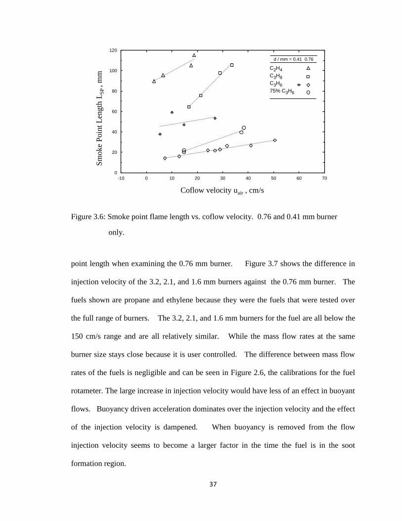
Figure 3.6: Smoke point flame length vs. coflow velocity. 0.76 and 0.41 mm burner

only……………………………………………………………………………...……….37

Figure 3.7: Smoke point flame length vs. fuel injection velocity. The linear fits are shown

for each burner diameter for a given fuel………………….……………………..………38

Figure 3.8: Smoke point flame length vs. Reynolds number based on fuel injection

velocity…………………………………………………………………………………...39

Figure 3.9: Standard pressure nonbuoyant methane smoke point lengths…………….…40

Figure 3.10: Standard pressure nonbuoyant ethane smoke points lengths………………41

Figure 3.11: Smoke point flame length vs. coflow velocity for ethylene and propane. The

linear fits are shown for each fuel. Ethylene and propane smoke lengths are relatively

similar except in 0.76 mm burner………………………..………………………………42

Figure 3.12: The derived fuel factor, Af with respect to NSP of normal gravity flames

from Li and Sunderland [7]……………………………………………….……………...43

Figure 3.13: Smoke point flame length and scaled correlation. Original correlation found

by Dotson………………………………...………………………………….…………...44

Figure 3.14: Smoke point flame length and scaled correlation. All of the data found from

the MSG was used to update the correlation………………………….…………………45

Table 3.2 The change in fuel factors from the original study to the current

study………………………………………………………………………………...……46

Figure 3.15: A comparison of the measured smoke point data to the correlated smoke

point data for ethylene…………………………………………………………….……..47


the MSG was used to update the correlation. Ethylene at the 0.76 mm burner not

included in this plot………………………………………………………………………48

Figure 3.17: Smoke point flame length against the mass flow rate of the given

fuel……………………………………………………..………………………..……….51

1

Chapter 1: Introduction

Soot is a topic in the fire and combustion research that is important yet not

completely understood. Incomplete combustion causes the production of soot. Radiation

from soot is what causes the human eye to see flame as a bright yellow to dull orange

color [1]. It can provide the light and warmth for which people build fires. However,

soot radiation also causes increases in heat loads and contributes to fire spread rates.

Fire spread rates are increased from radiation from the soot and can shorten the

Available Safe Egress Time (ASET) in fire situations. Increase in heat loads from

radiation is particularly a problem with engines because radiation can cause a loss in

efficiency and unexpected temperatures. Radiation heat losses in a conventional diesel

engine are around 1.1% of the total fuel energy [2]. In many fire situations soot radiation

contributes more than gaseous radiation to heat transfer [3]. Soot has significant adverse

health effects in long term and short term exposures [4]. Soot emissions correlate with

carbon monoxide, which is a major cause of death in fires [5]. Climate change and

glacier melting have been linked with soot concentrations at high elevations [6]. Soot is

an important topic in fire phenomena and continued research in soot formation can lead

to a better understanding of predicting and eventually controlling soot production.

1.1 Smoke Points

Laminar smoke points are the generally used measure of fuel sooting tendency in

diffusion flames. The laminar smoke point of the flame is the condition where the flame

2

is non sooting but is at the threshold of producing soot. Any increase in fuel flow rate

will cause the flame to emit soot [7]. Laminar smoke point properties are usually

measured from round buoyant jet diffusion flames with coflowing air. The length of the

flame at the smoke point is the indicator of the flames tendency to soot. A longer smoke

point length is a characteristic of a flame that produces less soot. Smoke points have

been measured for gaseous, liquid, and solid fuels. Currently there is ASTM1322

“Standard Test Method for Smoke Point of Kerosene and Aviation Turbine Fuels,” but

this standard applies to wick fed liquid fuels and not gas jet fuels. Smoke points of

gaseous fuels are found from a coflowing jet flame apparatus with excess of oxygen.

Gaseous fuels have been studied under normal gravity systems [8] as well as under

elevated pressures [9] to help understand flame systems. Testing smoke points under

elevated pressures is especially useful for combustion devices and gas turbines. Not only

for the function of the device, but also for the environmental concerns of fuel emissions

[9].

There are four commonly used explanations for the occurrence of smoke points

that are not mutually exclusive[10]. The first is a smoke point occurs when the soot

temperature reaches its critical temperature of 1300 K (1000 K for microgravity) before

its burnout [10, 11, 12]. Another explanation of smoke point is that the radiative loss

fraction increases until it reaches 0.2-0.4 for normal gravity or 0.4-0.6 for microgravity

with the increase of fuel flow rate [10, 13, 14, 15, 16, 17, 18]. The ratio of the luminous

length and the stoichiometric length increase with increased fuel flow until it reaches a

smoke point around two [10, 16, 19, 20]. Lastly the increase in flame residence time

also increases the time available for soot formation and oxidation. Longer residence

3

times can increase radiative loss fractions and the volume of radiating soot [10, 21].

Figure 1.1 shows a smoke point condition for an ethylene flame.

In normal gravity, laminar smoke points have been found to correlate with soot

volume fractions and radiative loss fractions of turbulent diffusion flames. This

connection is important for understanding the smoke production in turbulent flames.

Flames that have a longer laminar smoke point will have a lower soot formation rate.

Shorter smoke points indicate greater soot formation rates. The relationship between a

fuel’s peak soot formation rate and its laminar smoke point is being used for CFD

calculation of fire radiation [22]. Turbulent flow conditions are harder to model, but are

more useful in fire simulations.

Figure 1.1: Ethylene sooting flame

1.2 Soot Formation

Understanding the sooting tendencies of hydrocarbon fuels relative to one another

is important for the highly desired control of the fuels soot production. The tendency of

4

a flame to produce soot is strongly related to the type of flame, combustion process, and

other physical parameters. It is important to recognize that all of these factors contribute

to the flames tendency to soot. The fuels that have been tested in this study are non-

aromatic hydrocarbon fuels. Non-aromatic fuels undergoing a pure or oxidative pyrolysis

will form aromatic rings during combustion. Moss (1995) and Leung (1991) simplified

the formation of soot to four main mechanisms: nucleation, heterogeneous surface

growth, coagulation, and oxidation [23, 24, 25]. During the combustion process aromatic

rings are formed to create polycyclic aromatic hydrocarbons (PAHs). Hydrocarbons with

simple structures like methane are more difficult to thermally decompose than a more

complex hydrocarbon like ethylene [9]. In the thermal decomposition acetylene is

formed and combines to form benzene rings. Those benzene rings form together to make

PAHs. PAHs are products of incomplete combustion and are precursors to soot

formation [26]. These particles grow and eventually form into particle nuclei when large

enough. The growing particles coagulate increasing the size of the particles. PAHs

levels have been found to be higher in under ventilated fires that produce more smoke.

Once soot is formed, it needs time to oxidize in the upper parts of the flame [22]. As the

soot travels through the flame it is cooled to a point where it can no longer be oxidized

[23]. Soot formation and oxidation increase as temperature increases, but oxidation rate

increases faster with temperature.

Soot formation processes are different based on the structure of the process taking

place. It is important to understand the structure of the process, whether it be premixed,

coflowing flames, inverse coflowing flames, counter flowing diffusion flames, or shock

tubes. Buoyancy effects also need to be considered. Santoro studies of soot formation

5

in coannular diffusion flames showed that a characteristic of smoking flames were

“wings” or “horns” around the sides of the flame [34, 44]. These characteristic horns

were caused by intense nucleation and agglomeration in the toroidal zone near the base.

The soot formed in this toroidal zone is convected along streamlines towards the tip of

the flame. The horns are formed around the outside of the flame because of these

streamlines of soot. From Kent and Wagner’s [10, 27] research on soot temperatures,

flames start emitting soot when the soot temperature in the oxidation zone cools below

1300 K with the effects of buoyancy. Nonbuoyant flames were found by Urban [10, 28]

to have temperatures of 1000 K when a smoke point condition was reached. The

decrease in temperature for nonbuoyant flames is the result of radiative quenching

because of the increased residence times of nonbuoyant diffusion flames.

The most extensive work on sooting of laminar diffusion flames done by Schalla

[29, 40] showed that the sooting tendency decreases in the followed order: Aromatics >

Alkynes > Alkenes > Alkanes. Aromatics have already formed rings the transition

making them the most likely to soot. The bonding in the alkynes, alkenes, and alkanes

cause the difference in sooting for the nonaromatic fuels. Alkynes are the most likely to

form acetylene because of its triple bond. The formation of Acetylene is the fuel

intermediate leading to the precursors of soot formation [12]. Early data on the critical

sooting equivalence ratio for premix flames with air as the oxidizer showed that the

sooting tendency decreases in the followed order: Aromatics > Alkanes > Alkenes >

Alkynes [12, 36, 40]. Milliken’s research showed that the cooler the flame, the greater

the sooting tendency for premixed flames. This was later found to be true for diffusion

6

flames as well [12, 41, 42, 43]. Therefore to properly compare the fuel structure with the

sooting tendency, flame temperature needs to be controlled.

In diffusion flames oxygen and fuel meet in the reaction region, which is limited

by diffusion. Stoichiometry dictates the temperatures and location of the fuel reaction

region. Since stoichiometry is dominating over chemical kinetics in diffusion flame, soot

formation is simplified [22]. Soot formation/oxidation times are much greater than the

heat release reaction times so consideration only needs to be made for the diffusion times

and soot formation/oxidation time [22]. With soot formation/oxidation time being the

main factor in determining soot formation then controlling the residence times of the

flame becomes a controlling factor in soot production.

1.3 Flame Shapes

The flame shape is an important factor in the recognition of the smoke point. The

understanding of the soot formation areas and soot paths can help in the understanding of

soot formation. In buoyant flames, soot streamlines converge to the centerline where the

fuel is located, as seen in Figure 1.2. When fuel is increased so that a smoke point

condition is reached, the flame tip will change from a round tip to a sharp tip. In

nonbuoyant flames soot streamlines diverge from the nozzle axis [28]. In microgravity

the laminar smoke point condition can occur in two flame configurations: open-tip and

closed-tip flames. An open-tipped flame configuration is signified by a blunt tip that

occurs because there is no soot present at the flame’s axis. The reduction of flow

velocities and increase of radiative heat losses with increasing distance from the flame

7

base provide condition for quenching, and the opening of the tip. A closed-tipped flame

configuration occurs when radiative quenching is reduced at shorter residence times [18].

Open-tip flames were observed at large characteristic flame residence times with the

onset of soot emissions associated with radiative quenching near the flame tip. Closed-tip

flames have soot emissions along the flame axis and open-tip flames have soot emissions

form an annular ring about the flame axis [28, 30]. Figure 1.2 shows the soot paths as

well as the soot formation results. Soot formation in diffusion flames is limited to fuel-

equivalence ratios (φ) of 1-2 shown in Figure 1.2 [30]. For buoyant flames soot is

formed near the outside of the flame where φ=1 and then moves inward to the area of

cooler and higher fuel concentration. In nonbuoyant flames soot forms near the core

where φ=2 and is drawn out to the flame sheet. As nonbuoyant flames start to transition

to a smoke point condition they will develop the characteristic horns on the outer edge of

the flame sheet. The horns of a sooting flame can be seen in Figure 1.1.

Figure 1.2: Soot path lines through buoyant and nonbuoyant flames

8

1.4 Buoyancy Effects

Convection is the primary mode of transportation of soot in flames. Soot

movement is slightly affected by Brownian motion and temperature gradients [30]. The

difference between smoke point properties of nonbuoyant flames and buoyant ones are

due to the difference of hydrodynamic properties of the flames [21, 28, 30, 31, 32]. In

buoyant flames the flow is accelerating and the streamlines converge toward the axis of

the flame. The flow converges to the axis of the flame because of the fuel-rich flame

conditions. The difference in nonbuoyant flames is the flow is decelerating and the

soot leaves the flame over the extended flame region. The ratio of soot nucleation and

growth residence times to soot oxidations residence times are generally larger for buoyant

flames than nonbuoyant flames. Residences times are proportional to the square root of

flame length in buoyant flames [12, 21, 33]. For the nonbuoyant flames that Dotson

observed, residences times are not constant [10]. The soot pathlines can be seen in

Figure 1.2.

It is difficult to avoid buoyancy effects on earth even when using parabolic

aircrafts and drop facilities. Drop tests have limited test times and parabolic aircrafts have

g-jitter affecting microgravity smoke points for four different types of fuels in the

International Space Station [10]. Before smoke points were found for nonbuoyant jet

flames, it was thought that smoke points would not occur [12]. Urban reported that for

comparable flame conditions nonbuoyant smoke point lengths were up to 2.3 times

shorter than when tested in ground-based microgravity facilities and up to 6.4 times

shorter than buoyant smoke point lengths [30].

9

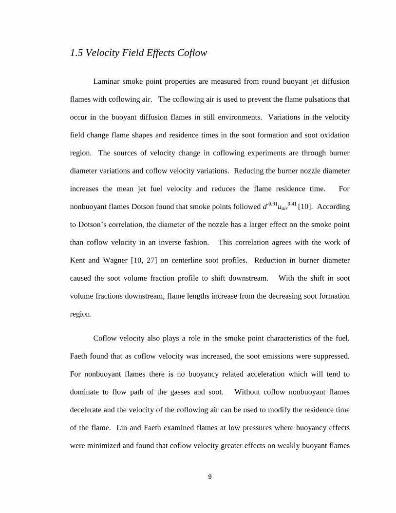
1.5 Velocity Field Effects Coflow

Laminar smoke point properties are measured from round buoyant jet diffusion

flames with coflowing air. The coflowing air is used to prevent the flame pulsations that

occur in the buoyant diffusion flames in still environments. Variations in the velocity

field change flame shapes and residence times in the soot formation and soot oxidation

region. The sources of velocity change in coflowing experiments are through burner

diameter variations and coflow velocity variations. Reducing the burner nozzle diameter

increases the mean jet fuel velocity and reduces the flame residence time. For

nonbuoyant flames Dotson found that smoke points followed d-0.91

uair0.41

[10]. According

to Dotson’s correlation, the diameter of the nozzle has a larger effect on the smoke point

than coflow velocity in an inverse fashion. This correlation agrees with the work of

Kent and Wagner [10, 27] on centerline soot profiles. Reduction in burner diameter

caused the soot volume fraction profile to shift downstream. With the shift in soot

volume fractions downstream, flame lengths increase from the decreasing soot formation

region.

Coflow velocity also plays a role in the smoke point characteristics of the fuel.

Faeth found that as coflow velocity was increased, the soot emissions were suppressed.

For nonbuoyant flames there is no buoyancy related acceleration which will tend to

dominate to flow path of the gasses and soot. Without coflow nonbuoyant flames

decelerate and the velocity of the coflowing air can be used to modify the residence time

of the flame. Lin and Faeth examined flames at low pressures where buoyancy effects

were minimized and found that coflow velocity greater effects on weakly buoyant flames

10

than buoyancy driven flames [27, 35, 38]. Their results did not result in a relation

between coflow velocity and smoke point length. A relationship between mass flow rate

and coflow velocity was found and is shown in Figure 1.3.

Figure 1.3: The effects of coflow velocity on mass flow rate [35, 38]

The increase in coflow reduced the soot volume fraction which increased the smoke point

length. Even in weakly buoyant flames of low pressure flames, the effects of buoyancy

driven acceleration changes the effect of coflow velocity. The effects of coflow

velocities on buoyant flames are less pronounced than nonbuoyant ones. Schalla and

McDonald [36] found that coflow velocity affect the fuel mass flow rate to a point and

then leveled off having no effect, as shown in Figure 1.4. This is consistent with the

11

Figure 1.4: The effect of coflow velocity on fuel flow rate [36, 38]

thoughts that buoyant flows dominate the velocity field. A study done by Berry-

Yelverton and Roberts [38, 39] showed that ethylene smoke point length increased while

the coflow increased. The decrease in the initial fuel to air velocity ratio was associated

with an increase in coflow velocity, which increased the smoke point length of ethylene.

Schalla and McDonald’s test were examined at fuel to air velocity ratios of 0.14 -0.42.

Berry-Yelverton and Roberts’s tests were done at higher fuel to air velocity ratios of 0.6

- 1.4 and can be seen in Figure 1.5. The effect of coflow velocity is different to buoyant

and nonbuoyant flames because of buoyancy driven acceleration. Without buoyancy

flames decelerate, as mentioned in the buoyancy discussion, and the effect of the coflow

velocity increased.

12

Figure 1.5 Ethylene smoke point length with respect to coflow velocity [38, 39]

1.6 SPICE HISTORY

The first smoke points were reported by Sunderland [21] in a microgravity

aircraft. Drop facilities were also used to obtain microgravity, but both had limitations

that caused difficulties in the acquisition of smoke point measurements. Urban [18],

realizing the time constraints of drop towers and the g-jitter associated with microgravity

aircrafts, measured smoke points in Earth’s orbit. The measurements were done in

quiescent air. Future work focuses on smoke points in coflowing air.

The Smoke Point in Co-flow Experiment (SPICE) goals are to acquire a: better

knowledge of and ability to predict heat release, soot production and emissions of fires in

microgravity; better design of combustors through improved control of soot formation;

13

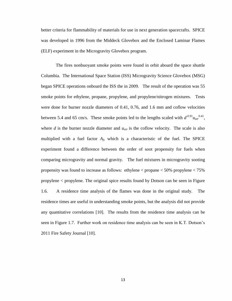
better criteria for flammability of materials for use in next generation spacecrafts. SPICE

was developed in 1996 from the Middeck Glovebox and the Enclosed Laminar Flames

(ELF) experiment in the Microgravity Glovebox program.

The fires nonbuoyant smoke points were found in orbit aboard the space shuttle

Columbia. The International Space Station (ISS) Microgravity Science Glovebox (MSG)

began SPICE operations onboard the ISS the in 2009. The result of the operation was 55

smoke points for ethylene, propane, propylene, and propylene/nitrogen mixtures. Tests

were done for burner nozzle diameters of 0.41, 0.76, and 1.6 mm and coflow velocities

between 5.4 and 65 cm/s. These smoke points led to the lengths scaled with d-0.91

uair0.41

,

where d is the burner nozzle diameter and uair is the coflow velocity. The scale is also

multiplied with a fuel factor Af, which is a characteristic of the fuel. The SPICE

experiment found a difference between the order of soot propensity for fuels when

comparing microgravity and normal gravity. The fuel mixtures in microgravity sooting

propensity was found to increase as follows: ethylene < propane < 50% propylene < 75%

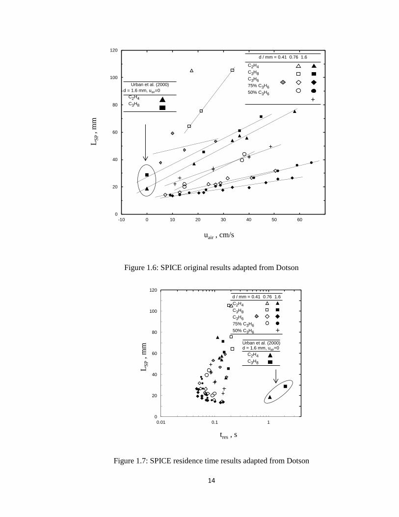
propylene < propylene. The original spice results found by Dotson can be seen in Figure

1.6. A residence time analysis of the flames was done in the original study. The

residence times are useful in understanding smoke points, but the analysis did not provide

any quantitative correlations [10]. The results from the residence time analysis can be

seen in Figure 1.7. Further work on residence time analysis can be seen in K.T. Dotson’s

2011 Fire Safety Journal [10].

14

Figure 1.6: SPICE original results adapted from Dotson

Figure 1.7: SPICE residence time results adapted from Dotson

0

20

40

60

80

100

120

-10 0 10 20 30 40 50 60 70

LS

P ,

mm

uair , cm/s

d = 1.6 mm, uair=0

C2H4

C3H8

Urban et al. (2000)

d / mm = 0.41 0.76 1.6

C2H4

C3H8

C3H6

75% C3H6

50% C3H6

+

0

20

40

60

80

100

120

0.01 0.1 1

LS

P ,

mm

tres , s

d = 1.6 mm, uair=0

C2H4

C3H8

Urban et al. (2000)

d / mm = 0.41 0.76 1.6

C2H4

C3H8

C3H6

75% C3H6

50% C3H6 +

15

1.7 Objectives and Contributions

The objective of the SPICE project is to get fundamental data on soot formation.

That data can be used in CFD soot models. Smoke point lengths are laminar tests that

correlate to soot volume fractions and radiative heat loss fractions in turbulent fires. The

smoke point lengths and their use in modeling can help provide an alternative to doing

expensive turbulent fire tests.

My contribution to the SPICE project was through video analysis and

interpretation of the data that was collected from the tests. The actual tests were done

by Don Pettit, a NASA astronaut, and were directed by Dr. David L. Urban. From the

videos, 57 new smoke points were found. This data that I collected will be combined

with the 2009 flight data throughout the following report. The 2009 data was interpreted

by Dotson in his completion of a M.S. in Fire Protection Engineering. Future work done

in the SPICE project should reference K.T. Dotson’s and my work for comparison of

results.

1.8 Computational Fluid Dynamics (CFD)

For CFD models to accurately predict fire growth there are necessary inputs for

characterization of the fire. Materials and geometric arrangements affect the burning

process. Turbulent buoyant jet flames would be an example of a characterization that is

used in CFD models. Delichatsios worked on simple correlations for the relationship

between laminar smoke point lengths and smoke yield in turbulent buoyant jet flames

16

[14]. Laminar smoke point lengths are related to soot volume fractions and radiant

fraction of flames. Using laminar data for turbulent flow is useful because of the

difficulty and unpredictability of turbulent tests. It is important to have fundamental data

set that can be used in these correlations. Since nonbuoyant flames are not driven by

buoyant forces, then there is one less parameter affecting the fundamental data. The Fire

Dynamics Simulator (FDS) and FireFoam are models that currently use laminar smoke

point lengths in correlations for turbulent conditions.

17

Chapter 2 Test Setup and Experimental Procedure

The Smoke Point In Co-flow Experiment (SPICE) tests were done in order to

determine a smoke point length for the various fuels burned. The transitions between

smoking and non-smoking flames were sometimes past the video’s field of view. The

transition between the smoking and non-smoking conditions are indicated by a few key

flame shapes. When a flame has transitioned into a smoking flame it changes from a

bright luminous rounded boundary at the flame tip to a flame tip with horns. The flame

tip opens up and becomes more of a red color because the soot is cooling for release. The

test setup and experimental procedure for the SPICE test is important. In order to ensure

that the data from the previous flights, the 2012 flight tests being examined, and future

flight tests can be compared the experimental procedure and test setup must remain

consistent.

2.1 SPICE

The SPICE operations were started in February 2009. The flames were observed

in the ISS Microgravity science box. The flames in the 2009 tests were successful and

showed a strong impact of the burner diameter and the co-flow air velocity. The strong

results called for a reflight and tests were done beginning in February 2012.

The Smoke Point In Co-flow Experiment Reflight (SPICE-R) tests were

conducted to expand the knowledge from the first tests. This expansion of knowledge

was meant for examining new fuels with a wider range of fuel diameters, as well as

18

expanding the statistical data that was gained from the first flight. The reflight dealt with

pure fuels of Ethane, Ethylene, Methane, and Propane at a range of 0.76-3.2 mm inside

burner diameters. The emphasis was to look at pure fuels where the 2009 flights

considered diluted fuels as well. The original SPICE burners had inside diameters of

0.41, 0.76, and 1.6 mm where the SPICE-R had 0.76, 1.6, 2.1, and 3.2 mm burners. The

SPICE test flight plans included the 0.4 mm burner, but there were no tests done with the

burner. The reflight tests were done by astronaut Don Pettit.

The rationale for the reflight was that the previous results have shown a strong

relationship with burner size and coflow velocity to microgravity smoke point lengths.

Normal gravity smoke points do not show such a strong relationship. Originally there

were only three burners tested, the largest being 1.6 mm. The increase in burner sizes to

2.1 and 3.2 mm burners would yield a larger number of smoke points with more fuels. In

the previous flight the effect of the burner diameter and coflow velocity was less known.

The knowledge gained from the previous flight helped with the creation of the test matrix

of the current study to maximize the number of smoke points that could be found.

2.2 Microgravity Science Glovebox

The redesign of the Middeck Glovebox, used in the Enclosed Laminar Flames (ELF)

experiment, led to the ISS Microgravity Science Glovebox. The glovebox, shown in

Figure 2.1, encapsulates the SPICE module where the flames are examined. The SPICE

experimental assembly, shown in Figure 2.2, is a rectangular duct that is approximately

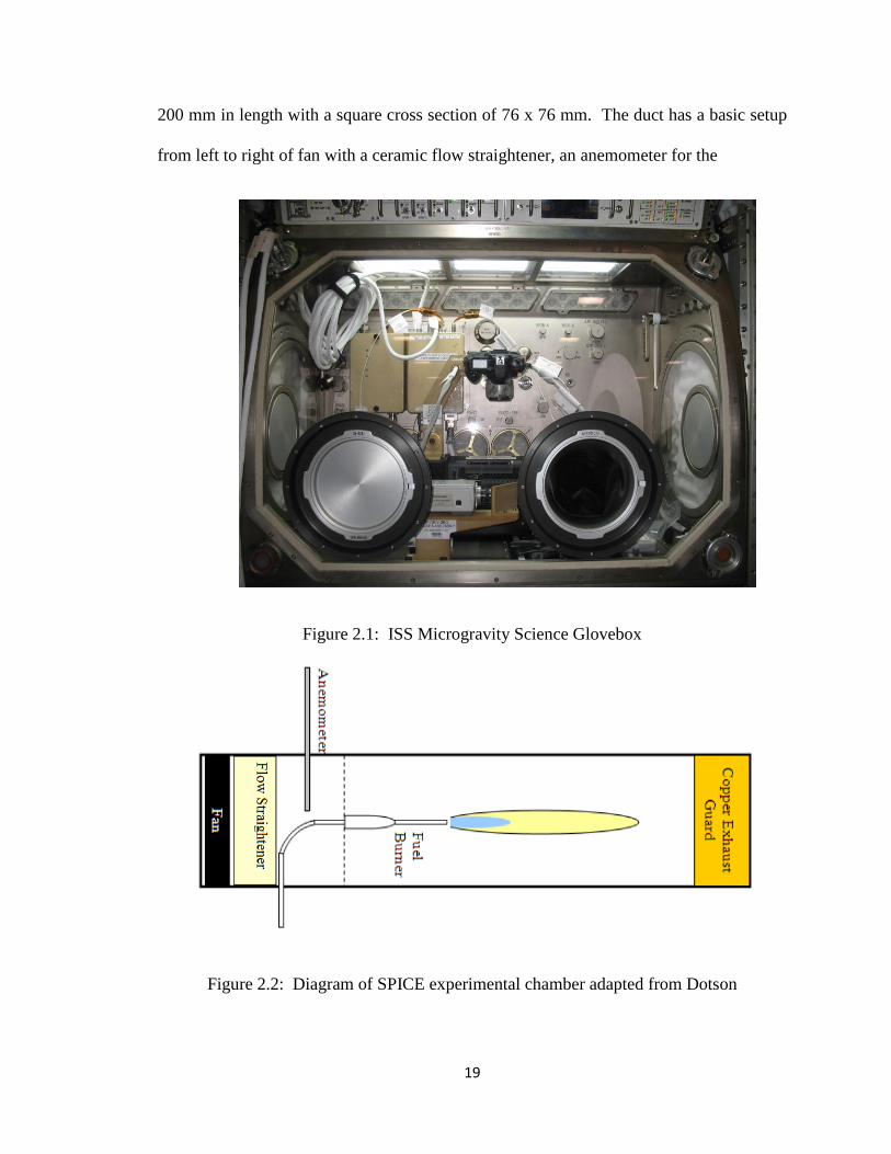
19

200 mm in length with a square cross section of 76 x 76 mm. The duct has a basic setup

from left to right of fan with a ceramic flow straightener, an anemometer for the

Figure 2.1: ISS Microgravity Science Glovebox

Figure 2.2: Diagram of SPICE experimental chamber adapted from Dotson

20

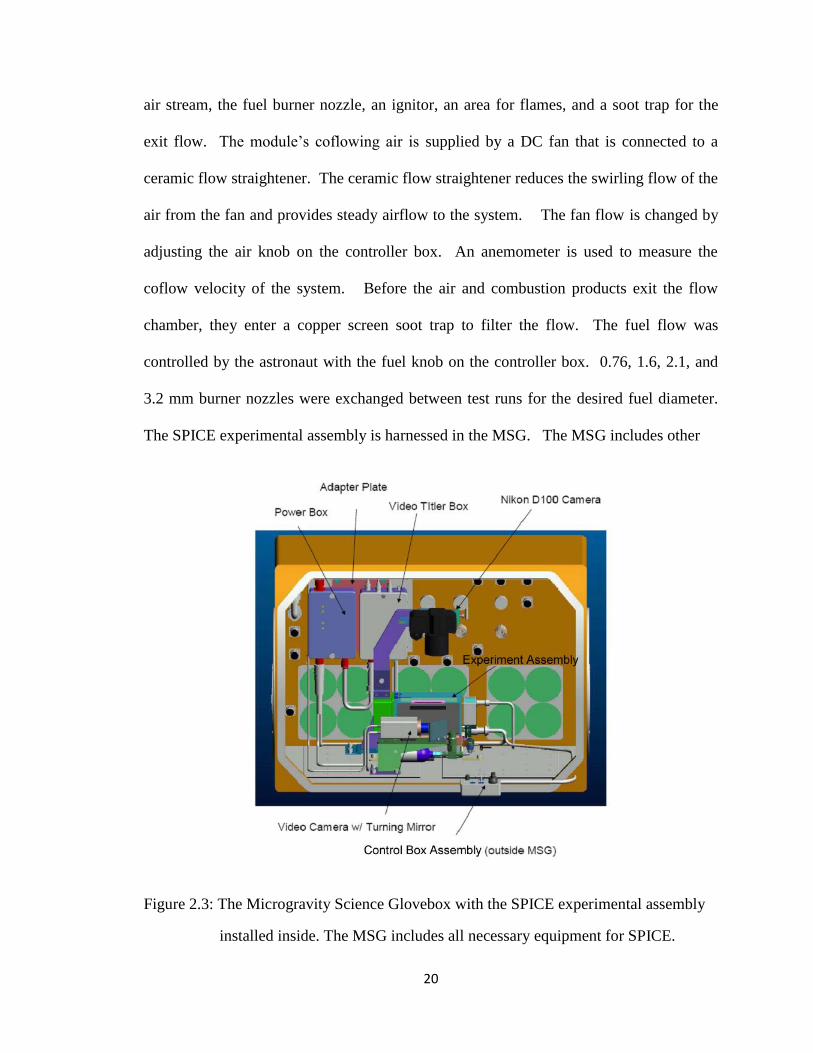
air stream, the fuel burner nozzle, an ignitor, an area for flames, and a soot trap for the

exit flow. The module’s coflowing air is supplied by a DC fan that is connected to a

ceramic flow straightener. The ceramic flow straightener reduces the swirling flow of the

air from the fan and provides steady airflow to the system. The fan flow is changed by

adjusting the air knob on the controller box. An anemometer is used to measure the

coflow velocity of the system. Before the air and combustion products exit the flow

chamber, they enter a copper screen soot trap to filter the flow. The fuel flow was

controlled by the astronaut with the fuel knob on the controller box. 0.76, 1.6, 2.1, and

3.2 mm burner nozzles were exchanged between test runs for the desired fuel diameter.

The SPICE experimental assembly is harnessed in the MSG. The MSG includes other

Figure 2.3: The Microgravity Science Glovebox with the SPICE experimental assembly

installed inside. The MSG includes all necessary equipment for SPICE.

21

equipment seen in figure 2.3. The MSG includes the SPICE experimental assembly, a

Nikon D100 Camera, a video camera, a control box, power box, and a video box. The

Nikon camera is there to supplement the video images with high resolution flame images.

The high resolution flame images are taken by the astronaut. The control box controls

the fan flow and the fuel flow in the experimental assembly.

The tests were first done test point by test point with ignitions before every test.

The astronaut would set the fan setting, adjust the fuel to a beginning setting, ignite the

flame, and adjust the fuel flow rate. The fuel flow rate would be adjusted until a smoke

point condition was reached. As the experiment progressed the astronaut became more

comfortable with the test procedure. Eventually multiple smoke points were found per

ignition without extinction of the flame. This procedure change was done in order to

save fuel for all of the test points. The ground support crew in Cleveland, OH was

guiding the astronaut through the tests indicating when to take pictures and when the

flame was smoking. The astronaut was eventually asked to indicate when the smoke

point condition occurred because he had the best view of the flame. The astronaut

indicated a smoke point conditions with an “elbow wiggle” for the second half of the

tests. Propane and a portion of ethane’s smoke point conditions were indicated by the

ground crew. The rest of the ethane, the methane, and the ethylene tests were all indicated

by the astronaut. A few test runs were done before the MSG was purged and cleaned of

the soot. The video was recorded on digital tapes. The videos were then matched up to

the audio and compressed into a multi-view video. The compressed videos contained

both the video of the MSG chamber and the video of the astronaut.

22

Once all of the tests were completed and the videos were compiled, the video and

camera images had to be analyzed for smoke point conditions. The smoke point

conditions were associated with the coflow rates from the video. The camera images,

although having much better quality, were not always at the smoke point condition.

Smoke point conditions were indicated by the scientists as well as identified through

characteristic qualities of a smoking flame. When the smoke point conditions were all

found their length were measured in Spotlight 16. Spotlight-16, a NASA created

software package, was designed to perform image analysis for images created by

microgravity combustion and fluid experiments. The flame endpoints were indicated by

the intensity. The endpoint of the flame was indicated by the intensity reaching fifty

percent of the bright yellow body of the flame. Further discussion of flame length

measurement can be found in the videography section 2.5.

2.3 Air Meter

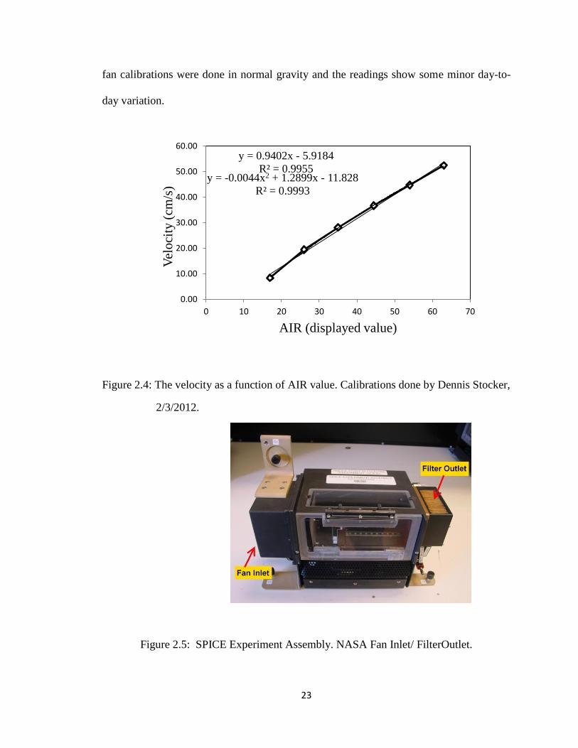
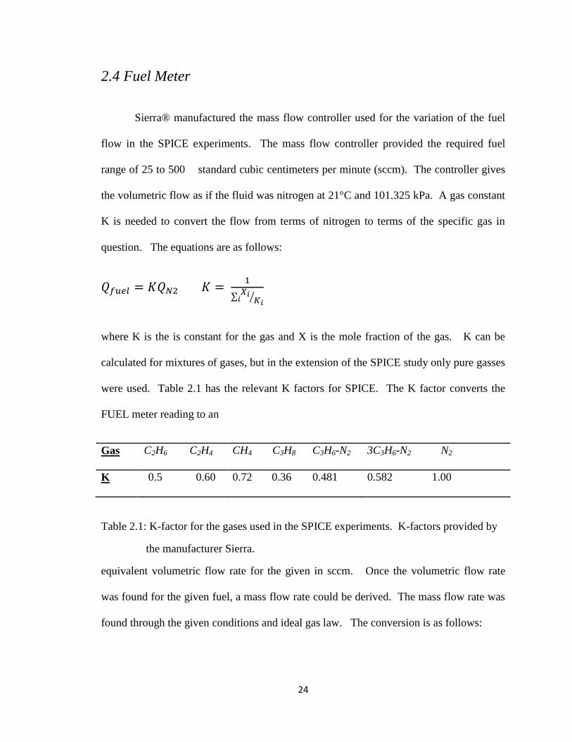
The SPICE flow duct anemometer measures the coflow velocity of the system.

The anemometer is located on the fan side of the glove box near the fuel burner shown in

Figure 2.2. The coflow flows through the SPICE experimental assembly shown in

Figure 2.5. The preflight fan calibration was done by Denis Stocker with the results

shown below in Figure 2.4. “AIR” reading is correlated to y = -0.0044x2 + 1.2899x -

11.828 in cm/s as shown in Figure 2.4. The fan provided co-flow velocities ranging from

5 to 50 cm/s. A knob that controls the coflow velocity adjusts the fan flow and changes

“AIR” and “FAN” readings on the MSG video display. It is important to note that the

23

fan calibrations were done in normal gravity and the readings show some minor day-to-

day variation.

Figure 2.4: The velocity as a function of AIR value. Calibrations done by Dennis Stocker,

2/3/2012.

Figure 2.5: SPICE Experiment Assembly. NASA Fan Inlet/ FilterOutlet.

y = 0.9402x - 5.9184

R² = 0.9955 y = -0.0044x2 + 1.2899x - 11.828

R² = 0.9993

0.00

10.00

20.00

30.00

40.00

50.00

60.00

0 10 20 30 40 50 60 70

Vel

oci

ty (

cm/s

)

AIR (displayed value)

24

2.4 Fuel Meter

Sierra® manufactured the mass flow controller used for the variation of the fuel

flow in the SPICE experiments. The mass flow controller provided the required fuel

range of 25 to 500 standard cubic centimeters per minute (sccm). The controller gives

the volumetric flow as if the fluid was nitrogen at 21°C and 101.325 kPa. A gas constant

K is needed to convert the flow from terms of nitrogen to terms of the specific gas in

question. The equations are as follows:

∑ ⁄

where K is the is constant for the gas and X is the mole fraction of the gas. K can be

calculated for mixtures of gases, but in the extension of the SPICE study only pure gasses

were used. Table 2.1 has the relevant K factors for SPICE. The K factor converts the

FUEL meter reading to an

Gas C2H6 C2H4 CH4 C3H8 C3H6-N2 3C3H6-N2 N2

K 0.5 0.60 0.72 0.36 0.481 0.582 1.00

Table 2.1: K-factor for the gases used in the SPICE experiments. K-factors provided by

the manufacturer Sierra.

equivalent volumetric flow rate for the given in sccm. Once the volumetric flow rate

was found for the given fuel, a mass flow rate could be derived. The mass flow rate was

found through the given conditions and ideal gas law. The conversion is as follows:

25

( )

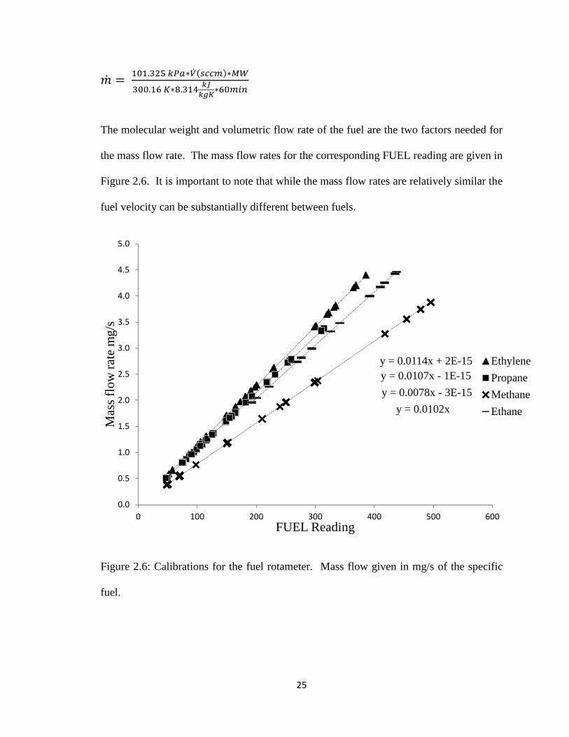
The molecular weight and volumetric flow rate of the fuel are the two factors needed for

the mass flow rate. The mass flow rates for the corresponding FUEL reading are given in

Figure 2.6. It is important to note that while the mass flow rates are relatively similar the

fuel velocity can be substantially different between fuels.

Figure 2.6: Calibrations for the fuel rotameter. Mass flow given in mg/s of the specific

fuel.

y = 0.0114x + 2E-15

y = 0.0107x - 1E-15

y = 0.0078x - 3E-15

y = 0.0102x

0.0

0.5

1.0

1.5

2.0

2.5

3.0

3.5

4.0

4.5

5.0

0 100 200 300 400 500 600

Mas

s fl

ow

rat

e m

g/s

FUEL Reading

Ethylene

Propane

Methane

Ethane

26

2.5 Videography

The image analysis was done in Spotlight-16, a NASA created software package

designed to perform image analysis for images created by microgravity combustion and

fluid experiments. Spotlight-16 is capable of performing analysis on single images or

sequences of images. Spotlight works with one or more subsets of the image that are

called an “Area Of Interest” (AOI). The main function used to find the smoke point

length was “Line Profile AOI.” The line profile has the ability to count the number of

pixels along that line and displays a graph of the intensities along the line. Besides

showing the intensity, the AOI can show the minimum, maximum, and mean intensities

along the line. The line profile function and luminance plot can be seen in Figure 2.7

Figure 2.7: Spotlight-16 Image analysis software. The flame lengths were measured by

pixel length. Luminance graph was used to find the end of the flame. The X

denotes when the luminosity is at the 50% of the maximum.

27

The line profile was used to determine the length of the smoke points observed.

Before the tests a ruler was shown as a reference to determine the pixel length

correlation. After determining the pixel length correlation, flame lengths were found

based on the number of pixels. An anchor was set at the end of the burner before each set

of tests that denoted the beginning of the flame. The end of the flame length was

determined by the intensity graph. When the intensity dipped below fifty percent it was

considered to be the end of the flame. An example of the flame length pixel correlation

can be seen in Figure 2.7. The pixel length correlation for the uncompressed video was

found to be 336.02 pixels per 70 mm. All of the videos were checked for accuracy before

measurements were taken.

2.6 Test Procedures

The test procedures for the smoke point flame test were predetermined by NASA.

The only part of the testing that differed from run to run was the number of flames that

were observed. As the astronaut became more comfortable with the test equipment and

procedures, more flames were observed in succession without extinguishment. The

succession of tests were performed in order to save fuel. Before each test the astronauts

were to refer to their execution notes for the test point number. Then the camera settings

were checked and adjusted as needed. The FUEL and FAN flow knobs were rotated to

the ignition values given by the test matrix. After the AIR value was verified as greater

than five then fuel and ignitor switches, on the SPICE control box assembly, were turned

28

to “ON”. Once the switches were turned to “ON” then the gas bottle valve must be

turned to “OPEN”. Opening the valve released the fuel and the ignitor was immediately

pulled forward until the flame appears. After the flame is lit the ignitor should be

released. On the SPICE control box assembly the FUEL flow was adjusted to find the

smoke point. Initially the procedure involved the ground scientist directing the astronaut

to the smoke point. Target points were given to the astronauts as seen in Figure 2.8.

Eventually the astronaut was directed to indicate when the smoke point occurred and did

Figure 2.8 Cues for the onset of smoke points for astronauts

29

so with a shoulder movement. At the smoke point the camera button was pushed, taking

a series of images. After the images were taken the FAN was adjusted to the next flow

in the run. This was repeated until all the smoke points were found in the run. After the

run or set of test points was finished the fuel and ignitor switch were turned off. The test

assembly was then setup for the next run.

30

Chapter 3 Results and Discussion

Smoke points were observed for four different fuels, including two fuels in which

smoke points were not previously found. A total of 57 smoke points were found to

double the previous study’s 55 smoke points to expand to a total of 112 smoke points

observed. Smoke point information from this study and Dotson’s study can be seen in

Appendix 5.1. Smoke points were found for methane and ethane along with more smoke

point data for propane and ethylene. In the previous microgravity study done by Dotson

smoke points were tested but smoke point conditions were not reached. The flames

would reach the copper plate at the end of the duct before approaching a smoke point

condition. Some of the fuels that produce less soot smoke points were too long to

examine all of the burner nozzle sizes. The smaller nozzles of 0.76 and 1.6 mm were not

examined or the tests failed to produce smoke points for methane and ethane. None of

the 0.4 mm burner tests were examined for the four fuels because the results would not

yield smoke points due to the length. The smoke point information is shown in Table

3.1. Flame images of the smoke points can be seen in the Appendix 5.2. Some of the

desired smoke point tests were planned for but not reached due to the limited supply of

fuel. There were some additional tests for the 3.2 mm burner of propane. A few of the

test points were thrown out due to a smoke point condition not being reached or the

smoke point was reached far out of the field of view. Five propane test points were lost

due to the flame not being brought to a smoking condition and one ethane smoke point

was past the field of view and could not be interpolated.

31

Fuel CH4 C2H6 C2H4 C3H8

d (mm) 3.2-2.1 3.2-1.6 3.2-0.76 3.2-0.76

uair (cm/s) 4.2-15.5 3.0-41.7 3.0-39.1 4.2-39.9

ufuel (cm/s) 66.2-170 19.9-180.3 10.1-714.2 8.4-389.1

Re (fuel) 123.9-211.6 94.7-387.5 36.6-683.1 57.4-788.5

LSP (mm) 75-97.5 44.2-112.1 20.8-115.2 26.5-97.7

Af (mm) 98.2 64.9 34.8 32.9

Number of Smoke

Points 6 13 19 19

Total number of

Smoke Points 6 13 25 25

Table 3.1 Results from the microgravity smoke points.

The transition of flames to their smoke points can be seen in Figure 3.1. Figure 3.1

shows the transition from the non-soot emitting flame to the soot emitting flames for the

four fuels. The smoke point for each sequence of flames is between the third and fourth

flame pictures. Figure 3.1 shows increasing fuel flow at a constant coflow velocity with

the increase in flame length for all of the fuels. The four fuels shows the dependence of

smoke point length on the type of fuel. Ethane and Methane have much longer smoke

points than the ethylene and propane at equivalent coflow velocities.

32

Figure 3.1: Flames at constant coflow and burner diameter with varying fuel flow rates

3.1 Coflow effects

The smoke point lengths are plotted against coflow velocity in Figure 3.2.

Smoke point data from the Dotson tests was added to the plot as well, representing all of

the microgravity smoke point data found in the SPICE. The linear fits indicate the smoke

point data for the given fuel and a given burner size with increasing coflow. Not all the

linear fits are increasing with coflow velocity at the same rate suggesting that there are

other contributing factors. The smaller burners and cleaner burning fuel increase more

33

rapidly with coflow velocity. One explanation could be that the increases in coflow

velocities decrease the residence time. The decrease in residence time decreases the

amount of time in the soot formation region causing less soot production. Another reason

for the increase in coflow leading to an increase in smoke point length is through soot

oxidation. Increases in coflow velocity could increase the rate of soot oxidation.

Coflow contributes less to smoke point length than burner diameter but is still a large

contributor and cannot be overlooked.

Figure 3.2: Smoke point flame length vs. coflow velocity. The linear fits are shown for

each burner diameter for a given fuel.

0

20

40

60

80

100

120

-10 0 10 20 30 40 50 60 70 80

Sm

ok

e P

oin

t L

ength

LS

P ,

mm

Coflow velocity uair , cm/s

d / mm = 0.41 0.76 1.6 2.1 3.2

CH4 C2H6 C2H4

C3H8

C3H6

75% C3H6

50% C3H6 +

34

3.2 Fuel Injection Velocity

Burner size is an important factor when discussing smoke points in microgravity.

Burner diameter controls the fuel inlet velocity which by examination of the correlation is

dominant over the coflow velocity. Smoke point length increases with decreasing burner

diameter. The decrease in diameter creates an increase in fuel jet injection velocity.

The increase in injection velocity pushes the centerline soot volume fraction downstream

Kent and Wagner’s research states [10, 27]. Fuel injection velocity is factored into the

residence times of that flame.

Figures 3.3-3.6 show the laminar smoke point lengths at the individual burner

diameters. Each plot has a different fuel tested at that individual burner. For the 1.6

mm burner six fuels were tested and given the most data. The plots follow decreasing

burner size and increasing fuel injection velocity. Figure 3.3 shows the 3.2 mm burner

Figure 3.3: Smoke point flame length vs. coflow velocity. 3.2 mm burner only.

0

20

40

60

80

100

120

-10 0 10 20 30 40 50 60 70

Sm

oke

Poin

t L

ength

LS

P ,

mm


d / mm = 3.2

CH4 C2H6 C2H4

C3H8

35

having a slight variation in slope from fuel to fuel with the exception of ethane. The

similar slopes throughout Figure 3.3 and 3.4 show that the effect of the coflow velocity is

very similar at low fuel injection velocities. Switching from fuel to fuel at a larger burner

diameter will not dramatically affect the rate of change of smoke point length with

coflow velocity. Injection velocities for the two burners range from 8.43 cm/s to 105.4

cm/s with methane being the outlier. The largest injection velocity at these two burners is

methane at 153.8 cm/s at the 2.1 mm burner. With only two test points found at the 2.1

mm burner for methane, it is hard to tell whether or not it would fit the same profile as

the rest of the fuels. More test points would be needed for methane to add to the analysis

of the 2.1 mm burner. Once the tests were switched to the 1.6 and 0.76 mm burners the


results started to produce outliers in changing smoke point length with respect to coflow

velocity. Ethane becomes the first fuel to not follow the trend of smoke point length

against injection velocity seen in Figure 3.5. It is expected that ethane would not follow

0

20

40

60

80

100

120

-10 0 10 20 30 40 50 60 70

Sm

oke

Poin

t L

ength

LS

P ,

mm


d / mm = 2.1

CH4 C2H6 C2H4

C3H8

36


the same path with coflow velocity because of its cleaner burning characteristics.

Besides ethane all of the fuels increase with coflow at a similar rate. The 0.76 and 0.41

mm burner, seen if Figure 3.6, is when the fuels do not follow the same path with

increasing coflow velocity. Ethylene and propane also switch in sooting propensity. At

the 0.76 mm burner injection velocities are much higher than previous burners and could

be a factor in the change in effect of the coflow velocity on smoke point length.

It is important to notice that there is an increasing change when decreasing the

size of the burner. The change in smoke point lengths between the 3.2 to 2.1 mm

burners is not as larger as the difference between the 1.6 and 0.76 mm burners. The

injection velocity doubles in the first change and is four times as much in the second

change. The fuel injection velocity is not linearly dependent with the change in burner

size. This nonlinear dependence can account for the degree of increase in the smoke

0

20

40

60

80

100

120

-10 0 10 20 30 40 50 60 70 80

Sm

oke

Poin

t L

ength

LS

P ,

mm


d / mm = 1.6

C2H6 C2H4

C3H8

C3H6

75% C3H6

50% C3H6 +

37

Figure 3.6: Smoke point flame length vs. coflow velocity. 0.76 and 0.41 mm burner

only.

point length when examining the 0.76 mm burner. Figure 3.7 shows the difference in

injection velocity of the 3.2, 2.1, and 1.6 mm burners against the 0.76 mm burner. The

fuels shown are propane and ethylene because they were the fuels that were tested over

the full range of burners. The 3.2, 2.1, and 1.6 mm burners for the fuel are all below the

150 cm/s range and are all relatively similar. While the mass flow rates at the same

burner size stays close because it is user controlled. The difference between mass flow

rates of the fuels is negligible and can be seen in Figure 2.6, the calibrations for the fuel

rotameter. The large increase in injection velocity would have less of an effect in buoyant

flows. Buoyancy driven acceleration dominates over the injection velocity and the effect

of the injection velocity is dampened. When buoyancy is removed from the flow

injection velocity seems to become a larger factor in the time the fuel is in the soot

formation region.

0

20

40

60

80

100

120

-10 0 10 20 30 40 50 60 70

Sm

oke

Poin

t L

ength

LS

P ,

mm


d / mm = 0.41 0.76

C2H4

C3H8

C3H6

75% C3H6

38

Figure 3.7: Smoke point flame length vs. fuel injection velocity. The linear fits are

shown for each burner diameter for a given fuel.

With higher injection velocities at smaller burner diameters it is important to

verify that the flow is not turbulent. The Reynolds number for each test is given by:

The Reynolds numbers were all under 1000 for the SPICE tests done. The Re < 1000

would suggest that the experiments never transitioned to turbulent flows. Figure 3.8

shows how the smoke point length over diameter changes with Reynolds number of the

fuel. The Reynolds of the fuel is driven by the diameter and the fuel injection velocity.

0

20

40

60

80

100

120

140

0 100 200 300 400 500 600 700 800

Sm

oke

Poin

t L

ength

(m

m)

Fuel injection velocity (cm/s)

d / mm = 0.41 0.76 1.6 2.1 3.2

C2H4

C3H8

39

Ethylene at the 0.76 mm burner is an outlier as seen in the other plots. Reynolds data can

be seen in Appendix 5.1.

Figure 3.8: Smoke point flame length vs. Reynolds number based on fuel injection

velocity.

3.3 Fuel comparison

Methane flames were the longest of the observed smoke point flames with the

largest Af value in the correlation. Tests of only 3.2 and 2.1 mm burners were able to be

examined at low coflow velocities. The maximum coflow velocity observed was 15.51

cm/s and can be seen in Figure 3.9. Even with the low coflow velocities the smoke

points were larger than the other fuels examined. The methane flames were less

luminous than their sooty counterparts. The flames grew in luminosity as they grew

0

20

40

60

80

100

120

140

160

0 100 200 300 400 500 600 700 800 900

Sm

ok

e P

oin

t L

ength

/ d

iam

eter

Reynolds Number, Re (fuel)

d / mm = 0.41 0.76 1.6 2.1 3.2

CH4 C2H6 C2H4

C3H8

C3H6

75% C3H6

50% C3H6 +

40

longer. Methane flames throughout the tests were open tipped flames. Their smoke

points were identified by the horns associated with smoke points. The horns are less

pronounced than other fuels because of the methane’s small propensity to create soot.

Figure 3.9: Standard pressure nonbuoyant methane smoke point lengths.

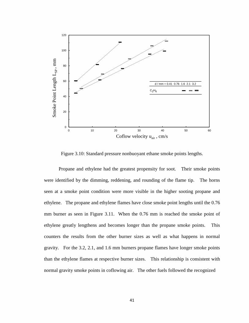
Ethane flames had the next longest smoke point lengths. Ethane smoke points

were tested for 3.2, 2.1 and 1.6 mm burners. The 1.6 mm burner tests began to pass the

edge of the field of view and the tests were stopped. Ethane flames were clean burning,

but were more luminous than the methane flames. The ethane smoke point was

signified by the transition to an open-tip flame with horns. As the coflow velocities

increased the smoke point condition came before the transition to an open-tipped flame.

The smoke point occurred when the flame was still closed tip. The smoke point was

recognized by the reddening of the flame tip. The decrease in burner size saw the same

result. In the 1.6 mm burner, closed tip smoke points occurred at much lower coflow

velocities. The ethane smoke point results are shown in Figure 3.10.

0

20

40

60

80

100

120

0 10 20

Sm

oke

Poin

t L

ength

LS

P ,

mm


d / mm = 0.41 0.76 1.6 2.1 3.2

CH4

41

Figure 3.10: Standard pressure nonbuoyant ethane smoke points lengths.

Propane and ethylene had the greatest propensity for soot. Their smoke points

were identified by the dimming, reddening, and rounding of the flame tip. The horns

seen at a smoke point condition were more visible in the higher sooting propane and

ethylene. The propane and ethylene flames have close smoke point lengths until the 0.76

mm burner as seen in Figure 3.11. When the 0.76 mm is reached the smoke point of

ethylene greatly lengthens and becomes longer than the propane smoke points. This

counters the results from the other burner sizes as well as what happens in normal

gravity. For the 3.2, 2.1, and 1.6 mm burners propane flames have longer smoke points

than the ethylene flames at respective burner sizes. This relationship is consistent with

normal gravity smoke points in coflowing air. The other fuels followed the recognized

0

20

40

60

80

100

120

0 10 20 30 40 50 60

Sm

ok

e P

oin

t L

ength

LS

P ,

mm


d / mm = 0.41 0.76 1.6 2.1 3.2

C2H6

42

Figure 3.11: Smoke point flame length vs. coflow velocity for ethylene and propane.

The linear fits are shown for each fuel. Ethylene and propane smoke

lengths are relatively similar except in 0.76 mm burner.

order of smoking diffusion flames: Aromatics > Alkynes > Alkenes > Alkanes. Ethylene

does not follow the conventional form for a 0.76 mm burner in nonbuoyant conditions

and its mechanisms need to be examined for a better understanding of the result.

The sooting propensity based on the derived Af values is as follows from least to

greatest propensity: methane (98.2) < ethane (64.9) < ethylene (34.8) < propane (32.8) <

50% propylene (20.04) < 75% propylene (12.15) < propylene (10.37). Values for

propylene were rederived based on their new fit in the correlation. The order of sooting

propensity is contradictory with normal gravity, which is discussed in the following

0

20

40

60

80

100

120

-10 0 10 20 30 40 50 60 70

Sm

ok

e P

oin

t L

ength

LS

P ,

mm


d / mm = 0.76 1.6 2.1 3.2

C2H4

C3H8

43

section. Normal gravity tests yield the results: methane < ethane < propane < ethylene <

50% propylene < 75% propylene < propylene. The Af values with respect to normalized

1g gravity smoke points can be seen in Figure 3.12. The normalized smoke point lengths

were obtained from Li and Sunderland [1]. It is important to note that ethylene has a

larger Af value than propane while having a shorter normalized smoke point length.

Figure 3.12: The derived fuel factor, Af with respect to NSP of normal gravity flames

from Li and Sunderland [7].

3.4 Correlation

The original correlation of smoke point was of the form

, where

d is in mm, a and b are fitted constants, uair is in cm/s, and Af is a constant derived for

each fuel in mm. Data from Dotson’s previous study was combined with the current

0

10

20

30

40

50

60

70

0 50 100 150 200 250 300 350

Af,

m

m

Normalized Smoke Point NSP, mm (1 g)

C2H6 C2H4

C3H8

C3H6

44

study to update the correlation. The correlation quantifies smoke point length’s

dependence of burner diameter, coflow velocity, and fuel. The a, b, and Af values were

determined from maximizing the R2 of the fit while the slope of the fit remained a

constant one. Once the exponents a and b were set the fuel Af was found by maximizing

the R2 value of the correlation. The original study done by Dotson lead to the a= - 0.910

b= 0.414 values used for smoke point length estimation. The exponent’s respective

signs of positive and negative are consistent with the previously discussed effects of

coflow and diameter change. As more fuels and data were added and more data was

added that correlation was no longer applicable. The original correlation done by

Dotson can be seen in Figure 3.13.

Figure 3.13: Smoke point flame length and scaled correlation. Original correlation found

by Dotson.

y = 1.00x R² = 0.90

0

20

40

60

80

100

120

-10 0 10 20 30 40 50 60 70 80 90 100 110

LS

P ,

mm

Af ( d / mm ) -0.91 ( uair s/cm ) 0.41 , mm

d = 1.6 mm, uair=0

C2H4

C3H8

Urban et al. (2000)

d / mm = 0.41 0.76 1.6

C2H4

C3H8

C3H6

75% C3H6

50% C3H6 +

45

With two more fuels and more than double the original data the correlation had to

be updated to reflect the new data. The addition of the new smoke points brought the

original correlation R2 value to a value close to 0.8. The scaling can be seen in Figure

3.14 and it is important to mention that the data from Urban [18] is not included in the

statistical fit. The original format,

of the scaling was kept because of

its connection with the data. However, when the new data was analyzed new a, b, and Af


the MSG was used to update the correlation.

y = 1.000x R² = 0.873

0

20

40

60

80

100

120

-10 0 10 20 30 40 50 60 70 80 90 100 110 120

Sm

oke

Poin

t L

ength

L

SP ,

mm

Af ( d / mm ) -0.665 ( uair s/cm ) 0.272 , mm

d / mm = 0.41 0.76 1.6 2.1 3.2

CH4 C2H6 C2H4

C3H8

C3H6

75% C3H6

50% C3H6 +

d / mm = 0.41 0.76 1.6 2.1 3.2

CH4 C2H6 C2H4

C3H8

C3H6

75% C3H6

50% C3H6 +

d = 1.6 mm, uair=0

C2H4

C3H8

Urban et al. (2000)

d / mm = 0.41 0.76 1.6 2.1 3.2

CH4 C2H6 C2H4

C3H8

C3H6

75% C3H6

50% C3H6 +

46

values were determined from maximizing the R2 of the fit. The updated correlation

values found in this study are a= 0-.665 and b= 0.272. These updated exponents better

reflect the cumulative data set. The updated Af values can be seen in Table 3.2 along with

Fuel CH4 C2H6 C2H4 C3H8 50 % C3H8 75 % C3H8 C3H8

Af original N/A N/A 21.2 18.5 13.9 7.65 6.05

Af (mm) 98.21 64.92 34.8 32.88 20.04 12.15 10.37

Table 3.2 The change in fuel factors from the original study to the current study

the previously derived fuel factors. With the addition of new data, the R2 of the fit

reduce from 0.90 to 0.873 with the addition of the new data. The reduction in the R2

ofthe fit is to be expected because of the number of data points that were added. Another

factor to the reduction of the R2 value was the addition of more 0.76 mm ethylene smoke

points. The smoke points for ethylene at the 0.76 mm burn do not follow the correlation

well. The difference between the correlation for the ethylene smoke point length and

ethylene’s measured smoke point length can be seen in Figure 3.15. Ethylene was the

fuel that did not recognize the order of diffusion flames given earlier by Glassman [29].

Without the four Ethylene points in the 0.76 mm, the correlation could be refined to a R2

value of 0.93 seen in Figure 3.16. The exponents of the correlation would change to a= -

0.5 b= 0.34. The effect of coflow increases. This increase is because at the 0.76 mm

burner the diameter of the burner starts having a larger effect than previous burner sizes.

However, further testing would need to be done to find the dominating factors affecting

these test points. In Sunderland’s [38] method of normalizing smoke points propane has

47

the greater smoke point length. The differences in the fuel need to be examined

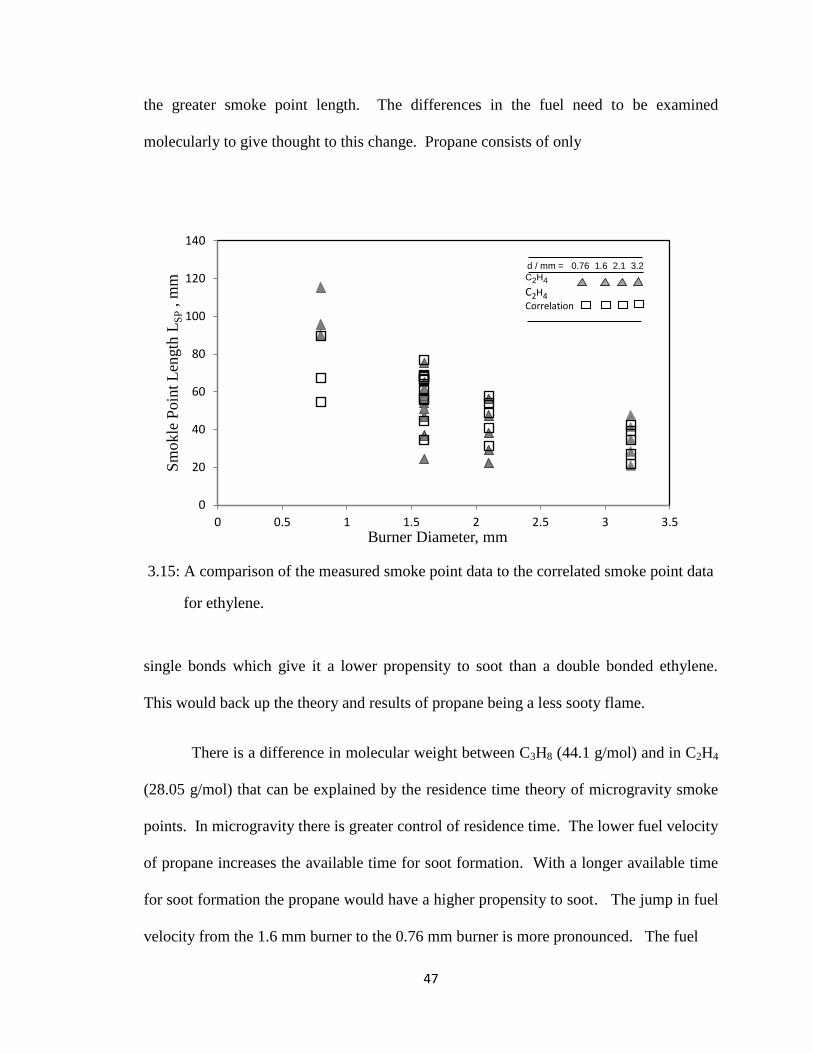
molecularly to give thought to this change. Propane consists of only

3.15: A comparison of the measured smoke point data to the correlated smoke point data

for ethylene.

single bonds which give it a lower propensity to soot than a double bonded ethylene.

This would back up the theory and results of propane being a less sooty flame.

There is a difference in molecular weight between C3H8 (44.1 g/mol) and in C2H4

(28.05 g/mol) that can be explained by the residence time theory of microgravity smoke

points. In microgravity there is greater control of residence time. The lower fuel velocity

of propane increases the available time for soot formation. With a longer available time

for soot formation the propane would have a higher propensity to soot. The jump in fuel

velocity from the 1.6 mm burner to the 0.76 mm burner is more pronounced. The fuel

0

20

40

60

80

100

120

140

0 0.5 1 1.5 2 2.5 3 3.5

Sm

okle

Poin

t L

ength

LS

P ,

mm

Burner Diameter, mm

d / mm = 0.76 1.6 2.1 3.2

C2H4

C2H4

Correlation

48


the MSG was used to update the correlation. Ethylene at the 0.76 mm burner

not included in this plot.

injection velocity from the 3.2 mm burner to the 2.1 mm burner increased by a factor of

two. In the transition from the 1.6 mm to the 0.76 mm burner the fuel velocity increased

by a factor of six. At the 1.6 mm burner the difference of injection velocities of ethylene

and propane is 40.78 cm/s-115 cm/s and 39.24-64.46 cm/s respectively. When switching

to the 0.76 mm burner the injection velocity of ethylene and propane increases to 551.07-

714.21 cm/s and 330.64-389.1 cm/s. The difference in the change in injection

y = 1.00x R² = 0.93

0

20

40

60

80

100

120

-10 0 10 20 30 40 50 60 70 80 90 100 110 120

Sm

okle

Po

int

Len

gth

LS

P , m

m

Af ( d / mm ) -0.5 ( uair s/cm ) 0.34 , mm

d = 1.6 mm, uair=0

C2H4

C3H8

Urban et al. (2000)

d / mm = 0.41 0.76 1.6 2.1 3.2

CH4 C2H6 C2H4

C3H8

C3H6

75% C3H6

50% C3H6 +

49

velocities as the burner diameter is minimized could account for the switch in sooting

propensity. Propane’s injection velocity is always smaller than ethylene but when

switching to the 0.76 mm burner the difference is 325 cm/s instead of around 50.5 cm/s

for the 1.6mm burner. The large difference in the injection velocity of the propane and

ethylene at the 0.76 mm burner gives propane a larger amount of time in the soot

formation region. Dotson did work to measure these residence times but the results were

inconclusive. Extensive research on residence times will provide some more differences

between the 0.76 mm and 1.6 mm burners.

The change in the correlation shows a few new thoughts about the contributors on

smoke points in microgravity. While burner size and diameter are still a dominating

factor in the smoke point length, it is not as pronounced as originally thought. The effect

of coflow decreased from 0.412 to 0.272 and the effect of burner size decreased from -

0.91 to -0.665. Both of the factors were scaled down by closely equivalent amounts with

coflow being scaled down slightly more. The decrease in the exponents of the

correlation was counteracted by the increase in fuel factors. The fuel factors all increased

by around thirty percent. The type of fuel is a larger factor in the smoke point length

than in the original correlation. The fuel should be a large factor in the correlation

because molecular shape has a large effect on a fuels sooting propensity. A fuel like

propane is cleaner burning than the double bonded propylene. According to Af values,

propylene (10.37) is more likely to produce soot than propane (32.88). The same is true

for ethylene and ethane. Ethylene (34.8) is more likely to produce soot than ethane

(64.92). Relating these fuel factors to a flame’s actual soot production would be the

next step. Further testing would need to be done to find out how much more an Af value

50

of 20 is to a value of 40. This kind of testing could be done through smoke sampling of

burning flames. The smoke point length is dominated by the fuel type and modified by

coflow velocity and burner size.

The correlation was thought up based on the controlling factors of the experiment.

There correlation was created because the dependence on one factor other than mass flow

rate could not be found. Mass flow rate dependence, seen in Figure 3.17, is expected

because of its relationship with smoke point length. This high R2 doesn’t provide any

explanation into smoke point lengths and their existence. Many different approaches

were tried for finding meaningful smoke point length plots. Residence times were

examined in Dotson’s work without the result of quantitative correlations. Radiative

losses of the flames were measured but those measurements were not reliable. Mass

flow rate over stoichiometric mixture fractions were examined as well in Dotson’s work

[38]. Further work on residence times and radiative loss fractions could provide some

insight on the controlling mechanisms of soot formation. The difficulty in finding

quantitative correlations for the smoke point length suggests that there may be multiple

contributing factors. The next step would be to find the level of contribution of these

factors. The four common smoke point explanations are: a smoke point occurs when the

soot temperature reaches its critical temperature of 1300 K (1000 K for microgravity)

before its burnout; a smoke point occurs when the radiative loss fraction increases until it

reaches 0.2-0.4 for normal gravity or 0.4-0.6 for microgravity; a smoke point occurs

when the ratio of the luminous length and the stoichiometric length increase with

increased fuel flow until it reaches a smoke point around two; a smoke point occurs

when the increase in flame residence time also increases the time available for soot

51

formation and oxidation. The definitions were discussed earlier as not being mutually

exclusive. There may be contributions from a number of factors discussed.

Figure 3.17: Smoke point flame length against the mass flow rate of the given fuel.

3.5 Procedures

The procedure is something that needs to be called into question when examining

smoke points in microgravity. It is important to remove any unnecessary source of error

in the data. The largest source of error that can come from these studies is the difference

of interpretation of a smoke point. The difference between a smoking and non-smoking

condition is not difficult to view, but is made more challenging when watching a

recording of the tests. The astronaut has a firsthand view of the smoking condition where

y = 24.449x

R² = 0.9604

0

20

40

60

80

100

120

140

0 0.5 1 1.5 2 2.5 3 3.5 4 4.5 5

Sm

oke

Poin

t L

ength

LS

P ,

mm

mass flow rate, mg/s

d / mm = 0.41 0.76 1.6 2.1 3.2

CH4 C2H6 C2H4

C3H8

C3H6

75% C3H6

50% C3H6 +

52

the people on the ground do not. Smoke points that are observed and indicated by the

astronaut or whoever has a firsthand view of the experiment will reduce the error

associated with the smoke points. The person with a firsthand view of the experiment

can explicitly see whether the flame is smoking or not.

It is more difficult to see smoke in the video version of the test. This may be due

to the quality of the video camera and an update in equipment would be beneficial. The

smoke point is the transition from smoking to non-smoking flame so small amounts of

smoke need to be observed. An astronaut better trained in what a smoke point condition

is would provide the best results. Towards the middle of the study the astronaut started

to indicate when the smoke point condition occurred with at shoulder movement. This

visual movement took away any ambiguity of when the flame was at its transition point.

Other visual cues, like an LED light, would be beneficial in the flame’s video. There

should also be a standard way of finding a smoke point condition. The clearest tests

were when the flame was brought past the smoke point and the fuel was slowly decreased

until a smoke point was reached. When approached from a smoking flame the transition

is more distinctive. Some of the tests were approached from the nonsmoking side and

the transition was not reached. Each data point is very important due to the environment

it takes to recreate the data.

53

Chapter 4 Conclusions

Microgravity smoke points of four different fuels were observed. Methane,

ethane, ethylene, and propane were observed with varying burner sizes of 0.76, 1.6, 2.1,

and 3.2 mm. A total of 57 smoke points were found to double the previous study of 55

smoke points to expand to 112 smoke points total. Previous work by Dotson emphasized

the relationship of microgravity smoke point length with burner size and coflow velocity.

Decreasing the burner diameter will increase the smoke point length. Increasing the

coflow velocity will increase the smoke point length. The increase in smoke point

lengths can be attributed to the change in residence times in the soot formation and soot

oxidation region. The increase in coflow velocities and reduction in burner diameter can

cause the soot volume fraction profile to shift downstream creating a longer smoke point

length. Previous work on residence time and soot formation time to soot oxidation time

ratio did not provide any relation between residence time and smoke points and was not

evaluated for the new data.

With the previous smoke point data collected by Dotson, the fuel sooting

propensity are shown as follows: methane < ethane < ethylene < propane < 50%

propylene < 75% propylene < propylene. The ranking is based on the Af values found

for the fuels, which can be found in Table 3.1. There is an exception in the 0.76 mm

burner for ethylene and propane. Propane produces less soot than ethylene in the 3.2,

2.1, and 1.6 mm, but ethylene is less sooty than propane in the 0.76 mm burner. This is

contrary to normal gravity studies where sooting propensity is as follows: methane <

ethane < propane < ethylene < 50% propylene < 75% propylene < propylene. In normal

54

gravity the propane fuel produces less soot in all cases. The switch in sooting

characteristics from the 1.6 to 0.76 mm burn could be a result of the fuel injection

velocity. The fuel injection velocity increases more in the change from the 1.6 to the

0.76 mm burner than any other burner change. The increase is so substantial that it

could account for the switch in sooting characteristics of the flames. Further testing

could be done to validate this effect. Similar fuel pairings to the ethylene/propane pairing

could be used to study this velocity effect. The important factor to consider is what the

0.76 mm burner and high injection velocities do to the fuels being studied.

Previously microgravity smoke points were scaled in the form

,

with a= - 0.910 b= 0.414. Given the work in the present study and the previous scaling

equation

, a and b were updated to a = -0.665 and 0.272. The updated

correlation involves two new fuels and 57 additional smoke points. The new correlation

comes with new fuel factors (Af). The Af values are increased by approximately 30

percent of the originally derived factors. The increase in Af values and decrease in a and

b values shows a greater dependence on the particular fuel type than previously found.

The a and b values decreasing show that their effect is less pronounced than originally

thought. However, the ratio of burner size and coflow velocity effect was very similar,

but each was scaled down. Even though the burner diameter and coflow velocity

decreased that does not diminish their effect. The two parameters are still controlling

factors in the length of the smoke point.

Methane smoke points were found for the first time at normal pressures. Since

methane produces less soot than other fuels, its smoke point is too long for normal

gravity tests. Methane’s simple structure makes it difficult to decompose into acetylene.

55

The methane smoke points nearly reached the edge of the field of view in the MSG with

coflow velocities up to 15.51 cm/s. Where in tests of other fuels in microgravity, coflow

velocities of up to 65 cm/s were used. With the addition of methane smoke points,

methane flames can be compared with the sooting of other fuels when it previously could

not.

This study does not prove the cause of smoke points or distinguish which of the

four commonly used mechanisms is dominant. This study provides fundamental data set

that can be used in CFD soot models. It has updated original correlations for smoke point

length correlations. A total of 57 smoke points were found to double the previous study

of 55 smoke points to expand to 112 smoke points total. Methane and ethane were two

new fuels observed, leading to the first standard pressure methane smoke points. There

were hopes in the experimentation to find the radiative losses at the smoke point

condition, but the data was not reliable. The results of the study will hopefully lead to a

better idea of smoke points and lead to further experiments distinguishing the dominant

mechanisms in sooting flames.

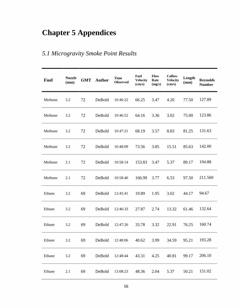
56

Chapter 5 Appendices

5.1 Microgravity Smoke Point Results

Fuel Nozzle

(mm) GMT Author

Time

Observed

Fuel

Velocity

(cm/s)

Flow

Rate

(mg/s)

Coflow

Velocity

(cm/s)

Length

(mm)

Reynolds

Number

Methane 3.2 72 DeBold 10:46:22 66.25 3.47 4.20 77.50

127.89

Methane 3.2 72 DeBold 10:46:52 64.16 3.36 3.02 75.00

123.86

Methane 3.2 72 DeBold 10:47:21 68.19 3.57 8.83 81.25

131.63

Methane 3.2 72 DeBold 10:48:09 73.56 3.85 15.51 85.63

142.00

Methane 2.1 72 DeBold 10:58:14 153.83 3.47 5.37 89.17

194.88

Methane 2.1 72 DeBold 10:58:40 166.99 3.77 6.53 97.50

211.560

Ethane 3.2 69 DeBold 12:45:41 19.89 1.95 3.02 44.17

94.67

Ethane 3.2 69 DeBold 12:46:33 27.87 2.74 13.32 61.46

132.64

Ethane 3.2 69 DeBold 12:47:26 33.78 3.32 22.91 76.25

160.74

Ethane 3.2 69 DeBold 12:48:06 40.62 3.99 34.59 95.21

193.28

Ethane 3.2 69 DeBold 12:48:44 43.31 4.25 40.81 99.17

206.10

Ethane 2.1 69 DeBold 13:08:23 48.36 2.04 5.37 50.21

151.02

57

Ethane 2.1 69 DeBold 13:08:57 66.65 2.82 14.42 69.17

208.12

Ethane 2.1 69 DeBold 13:09:34 82.28 3.48 25.95 88.96

256.95

Ethane 2.1 69 DeBold 13:10:09 98.64 4.17 35.50 106.04

308.05

Ethane 2.1 69 DeBold 13:10:31 105.38 4.45 41.67 112.08

329.09

Ethane 1.6 69 DeBold 14:22:15 92.01 2.26 3.02 60.42

218.92

Ethane 1.6 69 DeBold 14:23:00 121.85 2.99 12.21 81.67

289.92

Ethane 1.6 69 DeBold 14:23:36 162.89 4.00 21.88 110.83

387.55

Ethylene 3.2 83 DeBold 11:35:21 10.07 0.92 3.02 20.83

36.60

Ethylene 3.2 83 DeBold 11:35:48 13.30 1.22 6.53 28.33

48.35

Ethylene 3.2 83 DeBold 11:36:10 16.66 1.53 16.60 34.79

60.56

Ethylene 3.2 83 DeBold 11:36:31 20.89 1.91 26.94 41.25

75.92

Ethylene 3.2 83 DeBold 11:36:50 23.62 2.16 35.50 47.71

85.86

Ethylene 2.1 83 DeBold 11:06:29 21.65 0.85 4.20 22.08

51.65

Ethylene 2.1 83 DeBold 11:07:01 29.74 1.17 11.09 29.17

70.93

Ethylene 2.1 83 DeBold 11:07:34 38.98 1.54 20.84 37.92

86.08

Ethylene 2.1 83 DeBold 11:07:59 51.39 2.03 30.83 47.29

118.44

58

Ethylene 2.1 83 DeBold 11:08:32 58.90 2.32 39.08 56.25

140.48

Ethylene 1.6 83 DeBold 11:53:25 40.78 0.93 3.02 24.17

74.11

Ethylene 1.6 83 DeBold 11:53:45 61.67 1.41 7.68 36.46

112.07

Ethylene 1.6 83 DeBold 11:54:10 80.57 1.85 17.67 46.88

146.41

Ethylene 1.6 83 DeBold 11:54:31 94.00 2.15 24.94 51.04

170.82

Ethylene 1.6 83 DeBold 11:54:56 108.42 2.48 34.59 61.25

197.03

Ethylene 1.6 83 DeBold 11:55:12 115.88 2.65 37.31 65.00

210.59

Ethylene 1.6 45 Dotson 15:00:23 141.71 3.31 58.02 75.35

257.55

Ethylene 1.6 45 Dotson 14:37:08 102.93 2.41 33.57 53.99

187.07

Ethylene 1.6 45 Dotson 14:50:07 104.92 2.45 39.21 55.83

190.68

Ethylene 1.6 168 Dotson 9:49:13 103.92 2.43 36.39 57.50

188.87

Ethylene 1.6 45 Dotson 15:48:39 69.61 1.63 18.53 36.99

126.52

Ethylene 0.76 83 DeBold 12:18:08 551.07 3.16 3.02 89.79

527.07

Ethylene 0.76 83 DeBold 12:18:27 588.87 3.37 6.53 95.63

563.22

Ethylene 0.76 83 DeBold 12:19:00 714.21 4.09 18.74 115.21

683.09

Ethylene 0.76 45 Dotson 17:28:29 734.59 3.89 17.59 105.22

635.76

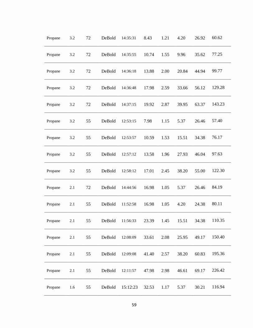
59

Propane 3.2 72 DeBold 14:35:31 8.43 1.21 4.20 26.92

60.62

Propane 3.2 72 DeBold 14:35:55 10.74 1.55 9.96 35.62

77.25

Propane 3.2 72 DeBold 14:36:18 13.88 2.00 20.84 44.94

99.77

Propane 3.2 72 DeBold 14:36:48 17.98 2.59 33.66 56.12

129.28

Propane 3.2 72 DeBold 14:37:15 19.92 2.87 39.95 63.37

143.23

Propane 3.2 55 DeBold 12:53:15 7.98 1.15 5.37 26.46

57.40

Propane 3.2 55 DeBold 12:53:57 10.59 1.53 15.51 34.38

76.17

Propane 3.2 55 DeBold 12:57:12 13.58 1.96 27.93 46.04

97.63

Propane 3.2 55 DeBold 12:58:12 17.01 2.45 38.20 55.00

122.30

Propane 2.1 72 DeBold 14:44:56 16.98 1.05 5.37 26.46

84.19

Propane 2.1 55 DeBold 11:52:58 16.98 1.05 4.20 24.38

80.11

Propane 2.1 55 DeBold 11:56:33 23.39 1.45 15.51 34.38

110.35

Propane 2.1 55 DeBold 12:08:09 33.61 2.08 25.95 49.17

150.40

Propane 2.1 55 DeBold 12:09:08 41.40 2.57 38.20 60.83

195.36

Propane 2.1 55 DeBold 12:11:57 47.98 2.98 46.61 69.17

226.42

Propane 1.6 55 DeBold 15:12:23 32.53 1.17 5.37 30.21

116.94

60

Propane 1.6 55 DeBold 15:13:13 48.04 1.73 14.42 44.38

169.51

Propane 1.6 55 DeBold 15:14:00 64.46 2.32 25.95 57.29

217.78

Propane 1.6 48 Dotson 16:54:27 82.34 3.03 44.85 71.38

296.07

Propane 1.6 48 Dotson 17:12:08 68.62 2.52 36.39 61.12

246.72

Propane 1.6 48 Dotson 17:45:17 48.93 1.80 22.29 45.52

175.93

Propane 0.76 55 DeBold 15:36:51 389.13 3.50 28.91 97.71

736.31

Propane 0.76 52 Dotson 11:39:28 460.49 3.84 33.57 105.45

788.45

Propane 0.76 52 Dotson 11:43:05 315.76 2.63 21.35 75.58

540.65

Propane 0.76 52 Dotson 11:49:43 271.03 2.26 16.65 64.33

464.06

50%

Propylene 1.6 55 Dotson 9:40:13 98.80 2.89 40.15 41.73

181.04

50%


137.77

50%


101.56

50%


136.89

50%


182.81

50%


206.66

50%


90.96

61

75%


144.12

75%


142.18

75%


113.17

75%


101.57

75%


76.41

75%


48.36

75%


47.39

75%


69.64

75%


50.30

75%


59.00

75%


302.65

75%


142.18

75%


138.12

75%


316.86


92.72


67.33

62


50.77


40.84


52.98


36.42


66.23


108.17


89.41


70.65


194.71


159.94


148.35


143.71


101.99


257.29


185.43


95.03

63


591.08


491.12


630.20


399.85

64

5.2 Flame Images and Information

Fuel C3H8 C3H8 C3H8 C3H8 C3H8

Nozzle 3.2 3.2 3.2 3.2 3.2

GMT 079 079 079 079 079

Time 14:35:31 14:35:55 14:36:18 14:36:48 14:37:15

Air (cm/s) 4.20 9.96 20.84 33.65 39.94

Length

(mm)

26.92 35.62 44.94 56.12 63.37

65

Fuel C3H8 C3H8 C3H8 C3H8

Nozzle 3.2 3.2 3.2 3.2

GMT 055 055 055 055

Time 12:53:15 12:53:57 12:57:12 12:58:12

Air (cm/s) 5.37 15.51 27.93 38.20

Length (mm) 26.46 34.38 46.04 55

66

Fuel C3H8 C3H8 C3H8 C3H8 C3H8 C3H8

Nozzle 2.1 2.1 2.1 2.1 2.1 2.1

GMT 055 079 055 055 055 055

Time 11:52:58 14:44:56 11:56:33 12:08:09 12:09:08 12:11:57

Air (cm/s) 4.20 5.37 15.51 25.95 38.20 46.61

Length (mm)

26.46 24.38 34.38 49.17 60.83 69.17

67

Fuel C3H8 C3H8 C3H8 C3H8

Nozzle 1.6 1.6 1.6 0.76

GMT 055 055 055 055

Time 15:12:23 15:13:13 15:14:00 15:36:51

Air (cm/s) 5.37 14.42 25.95 28.91

Length (mm) 30.21 44.38 57.29 97.71

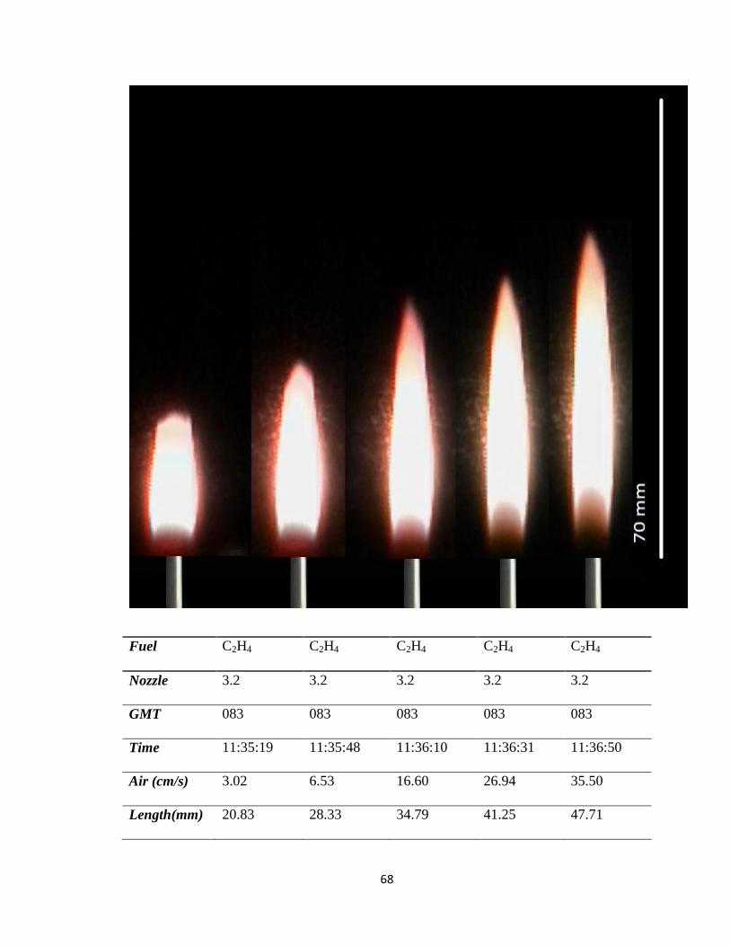
68


Nozzle 3.2 3.2 3.2 3.2 3.2

GMT 083 083 083 083 083

Time 11:35:19 11:35:48 11:36:10 11:36:31 11:36:50

Air (cm/s) 3.02 6.53 16.60 26.94 35.50

Length(mm) 20.83 28.33 34.79 41.25 47.71

69


Nozzle 2.1 2.1 2.1 2.1 2.1

GMT 083 083 083 083 083

Time 11:06:29 11:07:01 11:07:34 11:07:59 11:08:32

Air (cm/s) 4.20 11.09 20.84 30.83 39.08

Length

(mm)

22.08 29.17 37.92 47.29 56.25

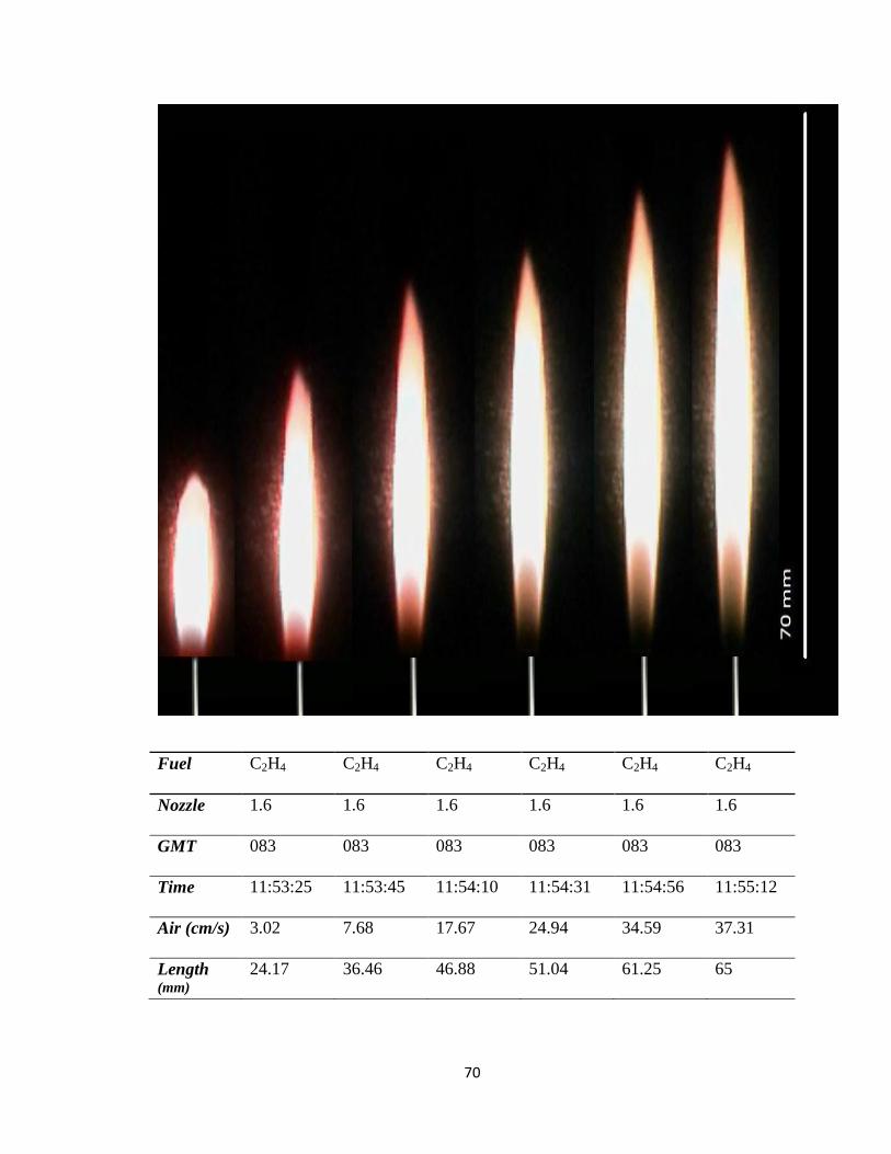
70

Fuel C2H4 C2H4 C2H4 C2H4 C2H4 C2H4

Nozzle 1.6 1.6 1.6 1.6 1.6 1.6

GMT 083 083 083 083 083 083

Time 11:53:25 11:53:45 11:54:10 11:54:31 11:54:56 11:55:12

Air (cm/s) 3.02 7.68 17.67 24.94 34.59 37.31

Length (mm)

24.17 36.46 46.88 51.04 61.25 65

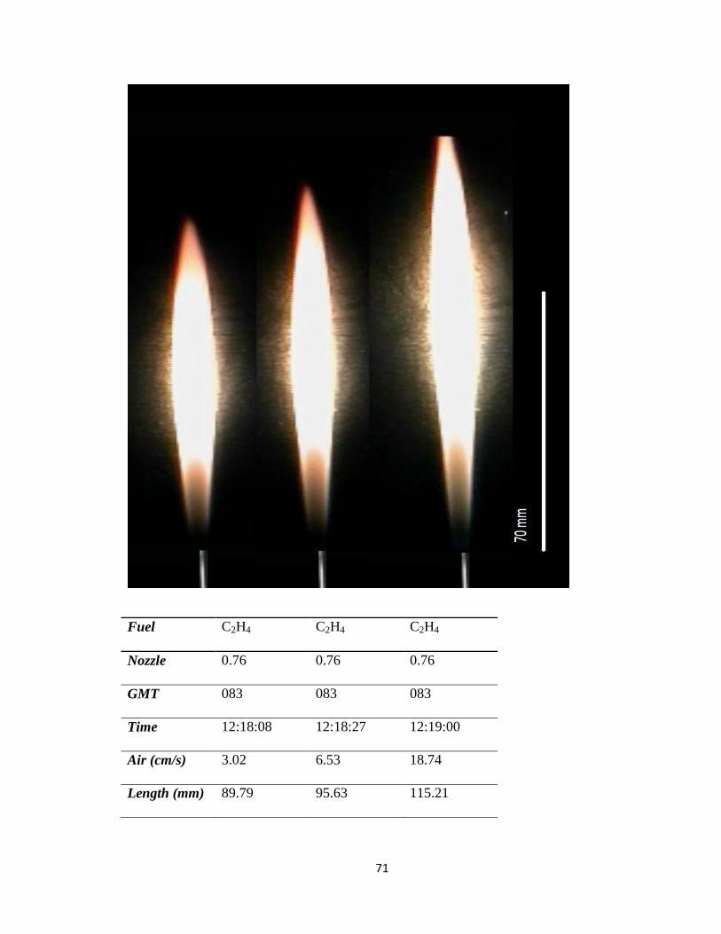
71

Fuel C2H4 C2H4 C2H4

Nozzle 0.76 0.76 0.76

GMT 083 083 083

Time 12:18:08 12:18:27 12:19:00

Air (cm/s) 3.02 6.53 18.74

Length (mm) 89.79 95.63 115.21

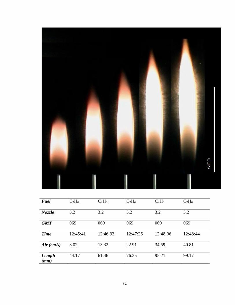
72


Nozzle 3.2 3.2 3.2 3.2 3.2

GMT 069 069 069 069 069

Time 12:45:41 12:46:33 12:47:26 12:48:06 12:48:44

Air (cm/s) 3.02 13.32 22.91 34.59 40.81

Length

(mm)

44.17 61.46 76.25 95.21 99.17

73


Nozzle 2.1 2.1 2.1 2.1 2.1

GMT 069 069 069 069 069

Time 13:08:23 13:08:57 13:09:34 13:10:09 13:10:31

Air (cm/s) 5.37 14.42 25.95 35.50 41.67

Length

(mm)

50.21 69.17 88.96 106.04 112.08

74

Fuel C2H6 C2H6 C2H6

Nozzle 1.6 1.6 1.6

GMT 069 069 069

Time 14:22:15 14:23:00 14:23:36

Air (cm/s) 3.02 12.21 21.88

Length (mm) 60.42 81.67 110.83

75

Fuel CH4 CH4 CH4 CH4 CH4 CH4

Nozzle 3.2 3.2 3.2 3.2 2.1 2.1

GMT 072 072 072 072 072 072

Time 10:46:22 10:46:52 10:47:21 10:48:09 10:58:14 10:58:40

Air (cm/s) 4.2 3.02 8.83 15.51 5.37 6.53

Length (mm)

77.5 75 81.25 85.63 89.17 97.5

76

References

[1] Turns, Stephen R., An Introduction to Combustion: Concepts and Applications. New

York: McGraw-Hill, Connect Learn Succeed, 2012. Print.

[2] Betrand, P., “Soot Formation of Lignin Derived Fuels In A Laminar Co-Flow

Diffusion Flame.” Report Number: WVT2009.09, 2009.

[3] Tien C.L., “Radiation Heat Transfer” SFPE Handbook of Fire Protection

Engineering, 4th

ed., edited by DiNenno, P. J., et al., National Fire Protection

Association, Quincy, MA, 2008, pp. 1-73-1-89.

[4] Kennedy, I.M., “The health effects of combustion-generated aerosols,” Proc.

Combust. Inst. 31 (2007) 2757–2770.

[5] Purser, D. A., “Assessment of Hazards to Occupants from Smoke, Toxic Gases, and

Heat,” SFPE Handbook of Fire Protection Engineering, 4th

ed., edited by DiNenno, P. J.,

et al., National Fire Protection Association, Quincy, MA, 2008, pp. 2-96-2-193.

[6] Ramanathan, V., and Carmichael, G., “Global and Regional Climate Change Due to

Black Carbon,” Nature Geoscience, Vol. 1, No. 4, 2008, pp. 221-227.

[7] Li, L., Sunderland, P.B., “An Improved Method of Smoke Point Normalization,”

Combustion Science and Technology 184 (2012) 829-841.

[8] Linteris, G. T., and Rafferty, I. P., “Flame Size, Heat Release, and Smoke Points in

Materials

Flammability,” Fire Safety Journal, Vol. 43, No. 6, 2008, pp. 442-450.

[9] Berry, T. L., and Roberts, W. L., “Measurement of Smoke Point in Velocity-Matched

Coflow

Laminar Diffusion Flames with Pure Fuels at Elevated Pressures,” Combustion and

Flame, Vol.

145, No. 3, 2006, pp. 571-578.

[10] Dotson, K.T., Sunderland, P.B., “Laminar Smoke Points of Coflowing Flames in

Microgravity.” Fire Safety Journal, Vol. 46, 2011.

[11] Kent, J.H. , Wagner, H.G., “Why do diffusion flames emit smoke?” Combust. Sci.

Technol. 41 (1984) 245–269.

[12] Glassman, I., “Soot Formation in Combustion Processes,” Twenty-Second

Symposium

(International) on Combustion, The Combustion Institute, Pittsburgh, PA, 1988, pp. 295-

311.

[13] Markstein,, G.H., “Relationship between smoke point and radiant emission from

buoyant turbulent and laminar diffusion flames,” Proc. Combust. Inst 20 (1984) 1055–

1061.

77

[14] M.A. Delichatsios, “Smoke yields from turbulent buoyant jet flames,” Fire Saf. J. 20

(4) (1993) 299–311.

[15] Delichatsios, M.A., “A phenomenological model for smoke-point and soot formation

in laminar flames,” Combust. Sci. Technol. 100 (1994) 283–298.

[16] Roper, F.G., Smith, C., “Soot escape from laminar air-starved hydrocarbon flames,”

Combust. Flame 36 (1979) 125–138.

[17] Markstein, G.H. , “Radiant emission and smoke points for laminar diffusion flames

of fuel mixtures,” Proc. Combust. Inst. 21 (1986) 1107–1114.

[18] D.L. Urban, Z.-G. Yuan, P.B. Sunderland, K.-C. Lin, Z. Dai, G.M. Faeth, “Smoke-

point properties of nonbuoyant round laminar jet diffusion flames,” Proc. Combust. Inst.

28 (2000) 1965–1972.

[19] Roper, F.G. “Soot escape from diffusion flames: a comparison of recent work in this

field,” Combust. Sci. Technol. 40 (1984) 323–329.

[20] Lin, K.-C., Faeth, G.M., Sunderland, P.B. , Urban, D.L., Yuan, Z.-G., “Shapes of

nonbuoyant round luminous hydrocarbon/air laminar jet diffusion flames,” Combust.

Flame 116 (1999) 415–431.

[21] Sunderland, P. B., Mortazavi, S., Faeth, G. M., and Urban, D. L., “Laminar Smoke

Points of

Nonbuoyant Jet Diffusion Flames,” Combustion and Flame, Vol. 96, No. 1-2, 1994, pp.

97-103.

[22] Lautenberger, C. W., de Ris, J. L., Dembsey, N. A., Barnett, J. R., and Baum, H. R.,

“A Simplified Model for Soot Formation and Oxidation in CFD Simulation of Non-

Premixed Hydrocarbon Flames,” AIAA Journal, Vol. 40, No. 2, 2005, pp. 141-176.

[23] Beji, T., Zhang, J. P., and Delichatsios, M., “Determination of Soot Formation Rate

from Laminar Smoke Point Measurements,” Combustion Science and Technology, Vol.

180, No. 5, 2008, pp. 927-940.

[24] Leung, K.M., Lindstedt, R.P., and Jones, W.P. (1991) “A simplified reaction

mechanism for

soot formation in nonpremixed flame.” Combust. Flame, 87, 289.

[25] Moss, J.B., Stewart, C.D., and Young, K.J. (1995) Modeling soot formation and

burnout in a high temperature laminar diffusion flame burning under oxygen-enriched

conditions.Combust. Flame, 101, 491.

[26] Tolocka, M.P., Miller, J.H. “Production of Polycyclic Aromatic Hydrocarbons fkom

Underventilated Hydrocarbon Diffusion Flames” Chemical and Physical Processes in

Combustion. Fall Technical Meeting, October 16-18, 1995, 253–256 pp, Worcester, MA.

78

[27] Lin, K.-C., Faeth, G.M., “Hydrodynamic suppression of soot emissions in laminar

diffusion flames,” J. Propul. Power 12 (1) (1996) 10–17.

[28] Urban, D. L., Yuan, Z.-G., Sunderland, P. B., Linteris, G. T., Voss, J. E., Lin, K.-C.,

Dai, Z., Sun,K., and Faeth, G. M., “Structure and Soot Properties of Nonbuoyant

Ethylene/Air Laminar Jet Diffusion Flames,” AIAA Journal, Vol. 36, No. 8, 1998, pp.

1346-1360.

[29] Glassman, Irvin. Combustion. New York: Academic, 2008. Print.

[30] Urban, D. L., Yuan, Z.-Y., Sunderland, P. B., Lin, K.-C., Dai, Z., and Faeth, G. M.,

“Smoke-Point Properties of Non-Buoyant Round Laminar Jet Diffusion” Proceedings of

the Combustion Institute, Volume 28, 2000, pp. 1965–1972

[31] Law, C. K., and Faeth, G. M., “Opportunities and Challenges of Combustion in

Microgravity” Prog. Energy Combust. Sci. 20:65–113 (1994).

[32] Kang, K.T., Hwang, J.Y., Chung, S.H., Lee, W., “Soot zone structure and sooting

limit in diffusion flames: comparison of counterflow and co-flow flames.” Combust.

Flame 109, 266–281.

[33] Sivathanu, Y. R., and Faeth, G. M., “Temperature / Soot Volume Fraction

Correlations in the Fuel-Rich Region of Buoyant Turbulent Diffusion Flames,”

Combustion and Flame, Vol. 81, No. 2, 1990, pp. 133-149.

[34] Santoro, R. J., Yeh, T. T., Horvath, J. J., and Semerjian, H. G., “The Transport and

Growth of Soot Particles in Laminar Diffusion Flames,” Combustion Science and

Technology, Vol. 53, No. 2, 1987, pp. 89-115.

[35] Lin, K.-C. and Faeth, G. M., “Shapes of Nonbuoyant Round Luminous Laminar-Jet

Diffusion Flames in Coflowing Air,” AIAA Journal, Vol. 37, No. 6, 1999, pp. 750-765.

[36] Schalla, R. L. and McDonald, G. E., “Mechanism of Soot Formation in Flames,”

Fifth Symposium (International) on Combustion, The Combustion Institute, Pittsburgh,

PA, 1955.

[38] Dotson, K.T., Sunderland, P.B. “Laminar Smoke Points of Coflowing Flames in

Microgravity.” University of Maryland, 2009.

[39] Berry Yelverton, T. L., Roberts, W. L., “Effect of Dilution, Pressure, and Velocity

on Smoke Point in Laminar Jet Flames,” Combustion Science and Technology, Vol.

180, No. 7, 2008, pp. 1334-1346.

[40] Schalla, R. L., Hibbard, R. R.: “’Smoke and Coke Formation in Combustion of

Hydrocarbon-Air Mixtures,” Chap. IX in NACA Report 1300, 1959.

[41] Venkat, C., Brezinsky, K., Glassman, I.: Nineteenth Symposium (International) on

79

Combustion, p. 143, The Combustion Institute,1982.

[42] Benson, S. W.: Twenty-First Symposium (International) on Combustion, p. 703, The

Combustion Institute, 1988.

[43] Frenklach, M.: “’On The Driving Force of PAH Production,” Twenty-Second

Symposium

(International) on Combustion The Combustion Institute, Pittsburgh, PA, 1988.

[44] Santoro, R. J., Semerjian, H. G., and Dobbins, R. A., “Soot Particle Measurements in

Diffusion Flames,” Combustion and Flame, Vol. 51, 1983, pp. 203-218.

ABSTRACT LAMINAR SMOKE POINTS OF COFLOWING …

Documents

Transcript of ABSTRACT LAMINAR SMOKE POINTS OF COFLOWING …