Abstract Interpretation Part I Mooly Sagiv Textbook: Chapter 4.
55
Abstract Interpretation Part I Mooly Sagiv Textbook: Chapter 4
-
date post
21-Dec-2015 -
Category
Documents
-
view
230 -
download
3
Transcript of Abstract Interpretation Part I Mooly Sagiv Textbook: Chapter 4.
Abstract InterpretationPart I
Mooly Sagiv
Textbook: Chapter 4
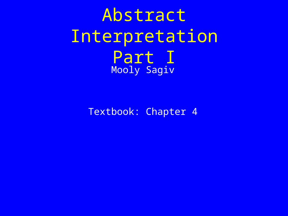
The Abstract Interpretation Technique (Cousot & Cousot)
The foundation of program analysis Defines the meaning of the information computed
by static tools A mathematical framework Allows proving that an analysis is sound in a local
way Identify design bugs Understand where precision is lost New analysis from old Not limited to certain programming style
Outline
Monotone Frameworks with Widening Galois Connections (Insertions) Collecting semantics The Soundness Theorem
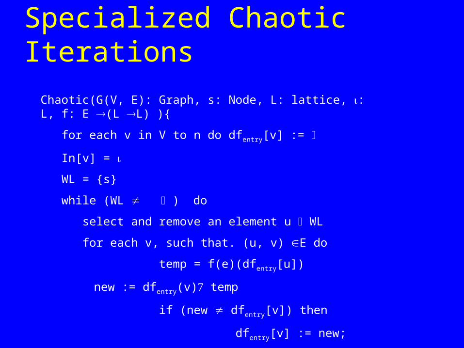
Specialized Chaotic Iterations
Chaotic(G(V, E): Graph, s: Node, L: lattice, : L, f: E (L L) ){
for each v in V to n do dfentry[v] :=
In[v] =
WL = {s}
while (WL ) do
select and remove an element u WL
for each v, such that. (u, v) E do
temp = f(e)(dfentry[u])
new := dfentry(v) temp
if (new dfentry[v]) then
dfentry[v] := new;
WL := WL {v}
Widening
Accelerate the termination of Chaotic iterations by computing a more conservative solution
Can handle lattices of infinite heights
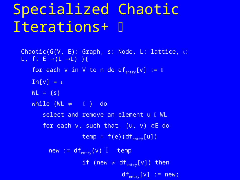
Specialized Chaotic Iterations+ Chaotic(G(V, E): Graph, s: Node, L: lattice, : L, f: E (L L) ){
for each v in V to n do dfentry[v] :=
In[v] =
WL = {s}
while (WL ) do
select and remove an element u WL
for each v, such that. (u, v) E do
temp = f(e)(dfentry[u])
new := dfentry(v) temp
if (new dfentry[v]) then
dfentry[v] := new;
WL := WL {v}
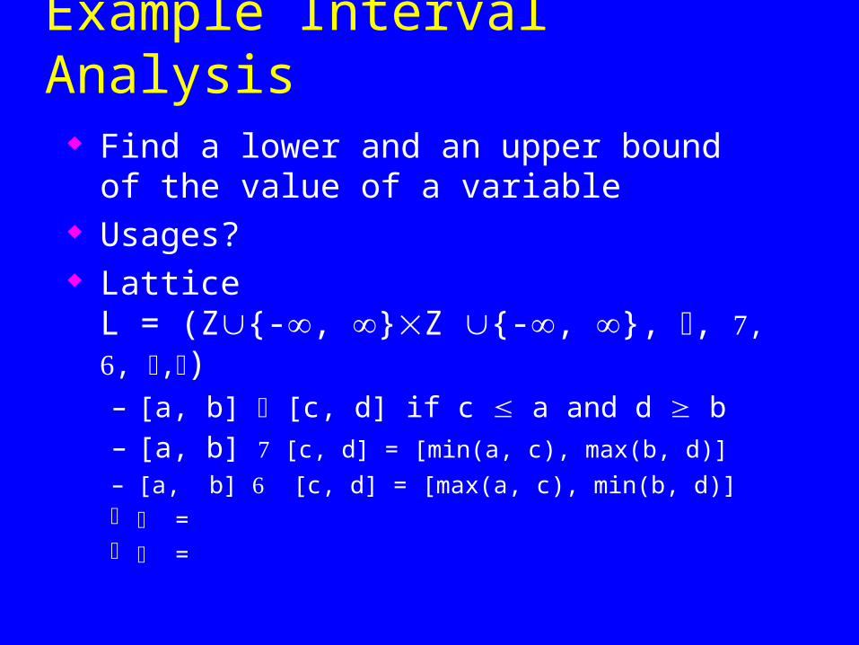
Example Interval Analysis Find a lower and an upper bound of the value of a
variable Usages? Lattice
L = (Z{-, }Z {-, }, , , , ,)– [a, b] [c, d] if c a and d b– [a, b] [c, d] = [min(a, c), max(b, d)]
– [a, b] [c, d] = [max(a, c), min(b, d)] = =
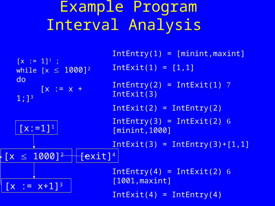
Example ProgramInterval Analysis
[x := 1]1 ;while [x 1000]2 do [x := x + 1;]3
IntEntry(1) = [minint,maxint]
IntExit(1) = [1,1]
IntEntry(2) = IntExit(1) IntExit(3)
IntExit(2) = IntEntry(2)
[x:=1]1
[x 1000]2
[x := x+1]3
[exit]4
IntEntry(3) = IntExit(2) [minint,1000]
IntExit(3) = IntEntry(3)+[1,1]
IntEntry(4) = IntExit(2) [1001,maxint]
IntExit(4) = IntEntry(4)
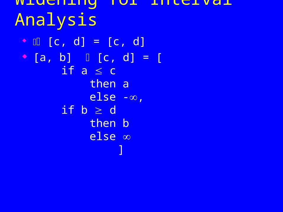
Widening for Interval Analysis [c, d] = [c, d] [a, b] [c, d] = [
if a cthen aelse -,
if b dthen belse
]
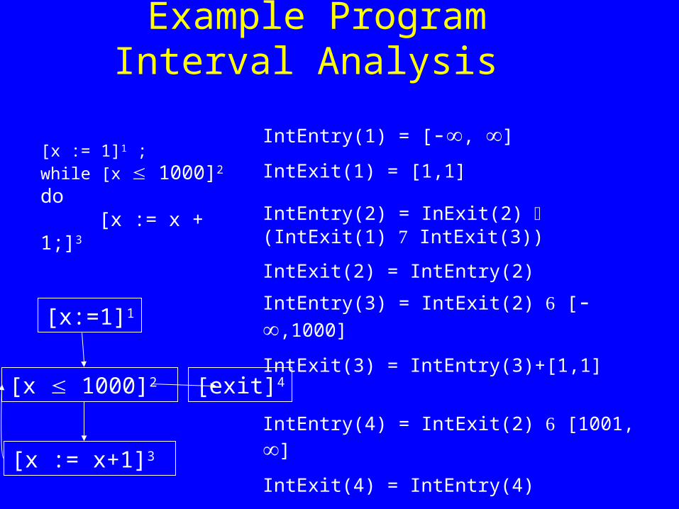
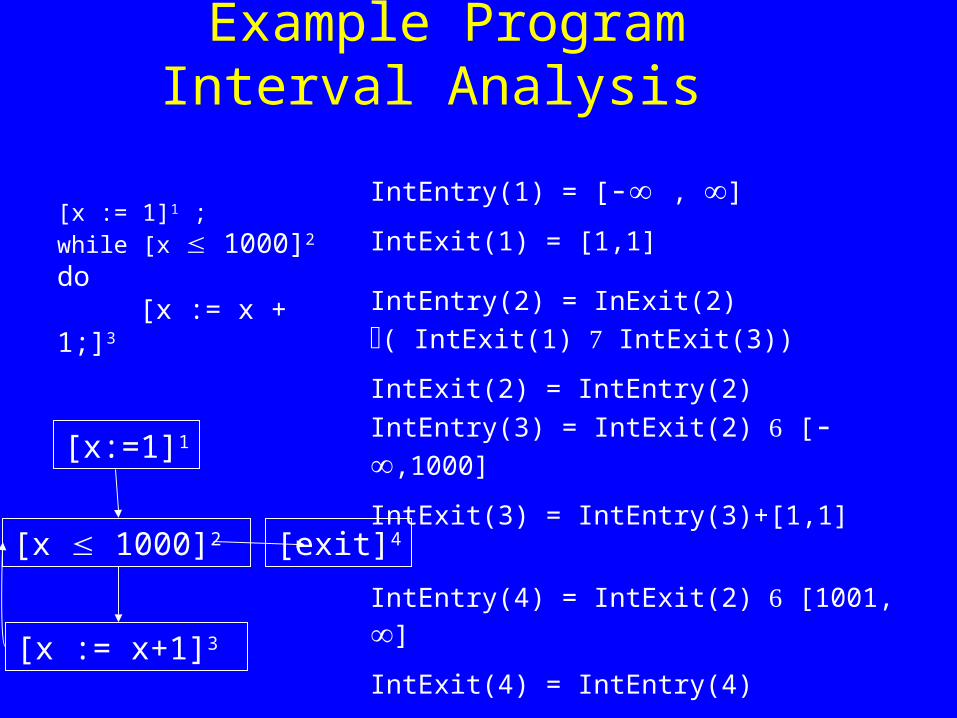
Example ProgramInterval Analysis
[x := 1]1 ;while [x 1000]2 do [x := x + 1;]3
IntEntry(1) = [-, ]
IntExit(1) = [1,1]
IntEntry(2) = InExit(2) (IntExit(1) IntExit(3))
IntExit(2) = IntEntry(2)
[x:=1]1
[x 1000]2
[x := x+1]3
[exit]4
IntEntry(3) = IntExit(2) [-,1000]
IntExit(3) = IntEntry(3)+[1,1]
IntEntry(4) = IntExit(2) [1001, ]
IntExit(4) = IntEntry(4)
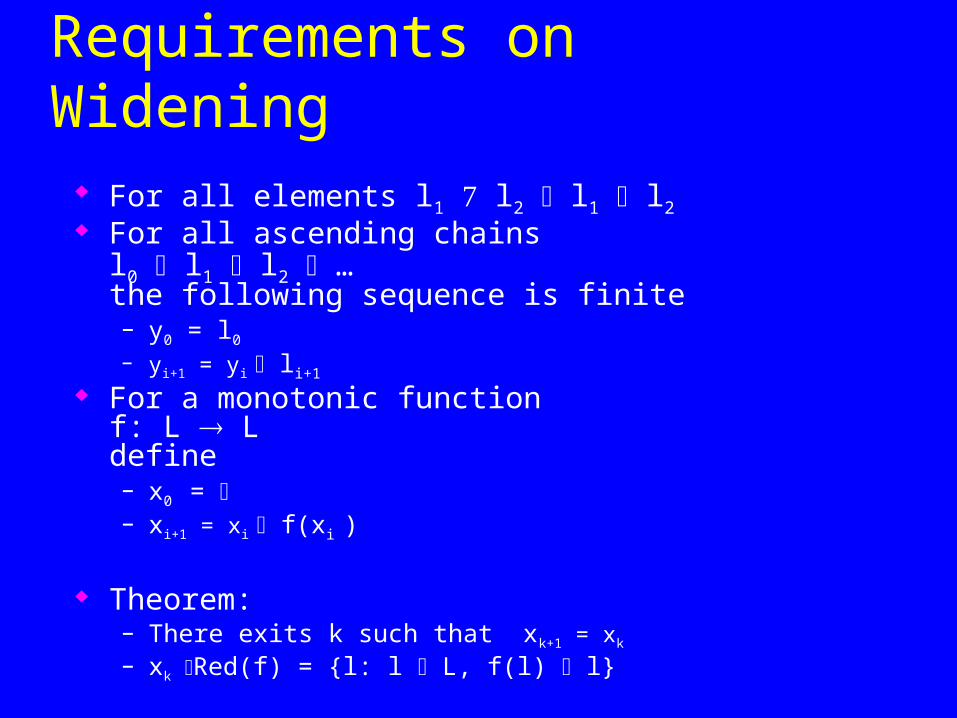
Requirements on Widening For all elements l1 l2 l1 l2 For all ascending chains
l0 l1 l2 …the following sequence is finite– y0 = l0 – yi+1 = yi li+1
For a monotonic function f: L Ldefine– x0 = – xi+1 = xi f(xi )
Theorem:– There exits k such that xk+1 = xk
– xk Red(f) = {l: l L, f(l) l}
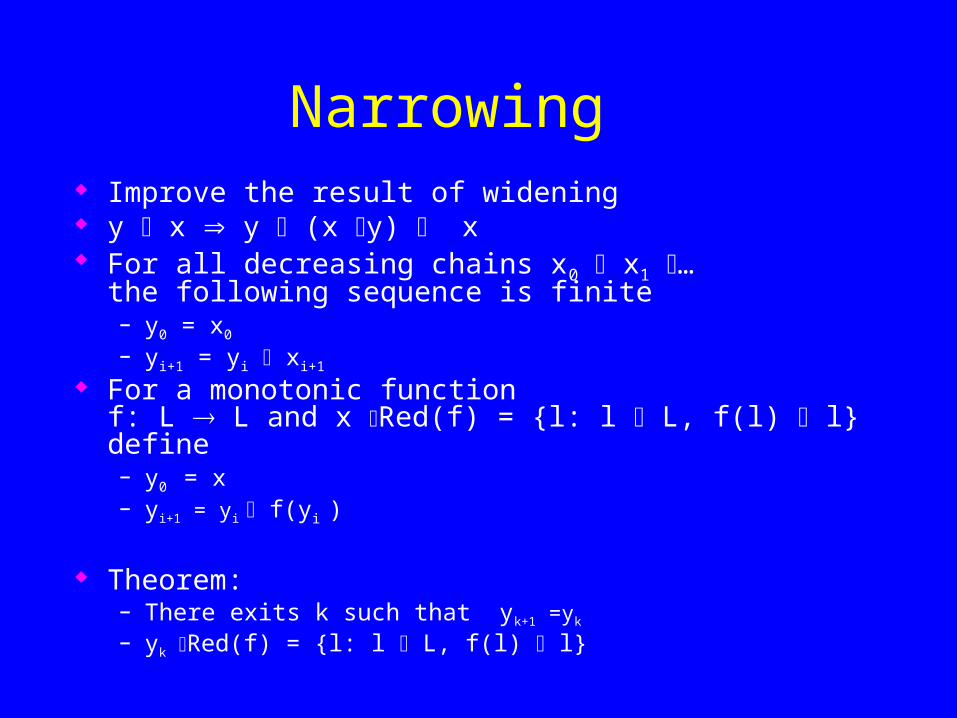
Narrowing Improve the result of widening y x y (x y) x For all decreasing chains x0 x1 …
the following sequence is finite– y0 = x0
– yi+1 = yi xi+1
For a monotonic function f: L L and x Red(f) = {l: l L, f(l) l}define– y0 = x– yi+1 = yi f(yi )
Theorem:– There exits k such that yk+1 =yk
– yk Red(f) = {l: l L, f(l) l}
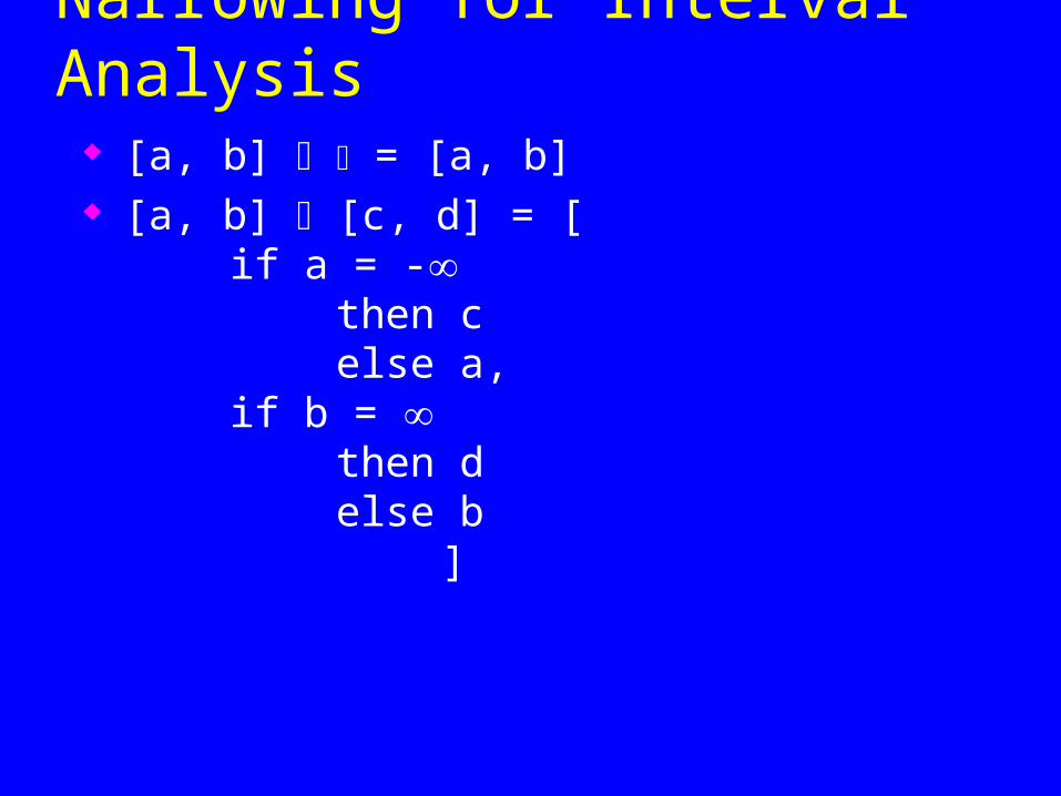
Narrowing for Interval Analysis [a, b] = [a, b] [a, b] [c, d] = [
if a = - then celse a,
if b = then delse b
]
Example ProgramInterval Analysis
[x := 1]1 ;while [x 1000]2 do [x := x + 1;]3
IntEntry(1) = [- , ]
IntExit(1) = [1,1]
IntEntry(2) = InExit(2) ( IntExit(1) IntExit(3))
IntExit(2) = IntEntry(2)
[x:=1]1
[x 1000]2
[x := x+1]3
[exit]4
IntEntry(3) = IntExit(2) [-,1000]
IntExit(3) = IntEntry(3)+[1,1]
IntEntry(4) = IntExit(2) [1001, ]
IntExit(4) = IntEntry(4)
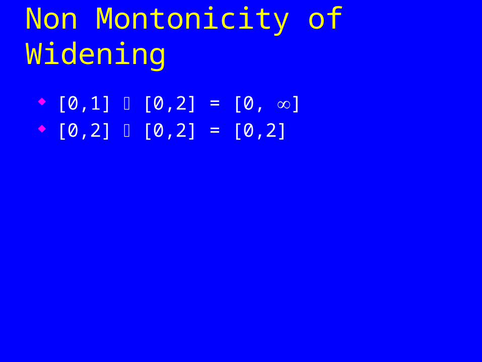
Non Montonicity of Widening
[0,1] [0,2] = [0, ] [0,2] [0,2] = [0,2]
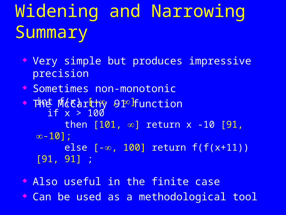
Widening and Narrowing Summary
Very simple but produces impressive precision Sometimes non-monotonic The McCarthy 91 function
Also useful in the finite case Can be used as a methodological tool
int f(x) [- , ] if x > 100 then [101, ] return x -10 [91, -10]; else [-, 100] return f(f(x+11)) [91, 91] ;
Foundation of Static Analysis
Static analysis can be viewed as interpreting the program over an “abstract domain”
Execute the program over larger set of execution paths
Guarantee sound results– Every identified constant is indeed a constant
– But not every constant is identified as such
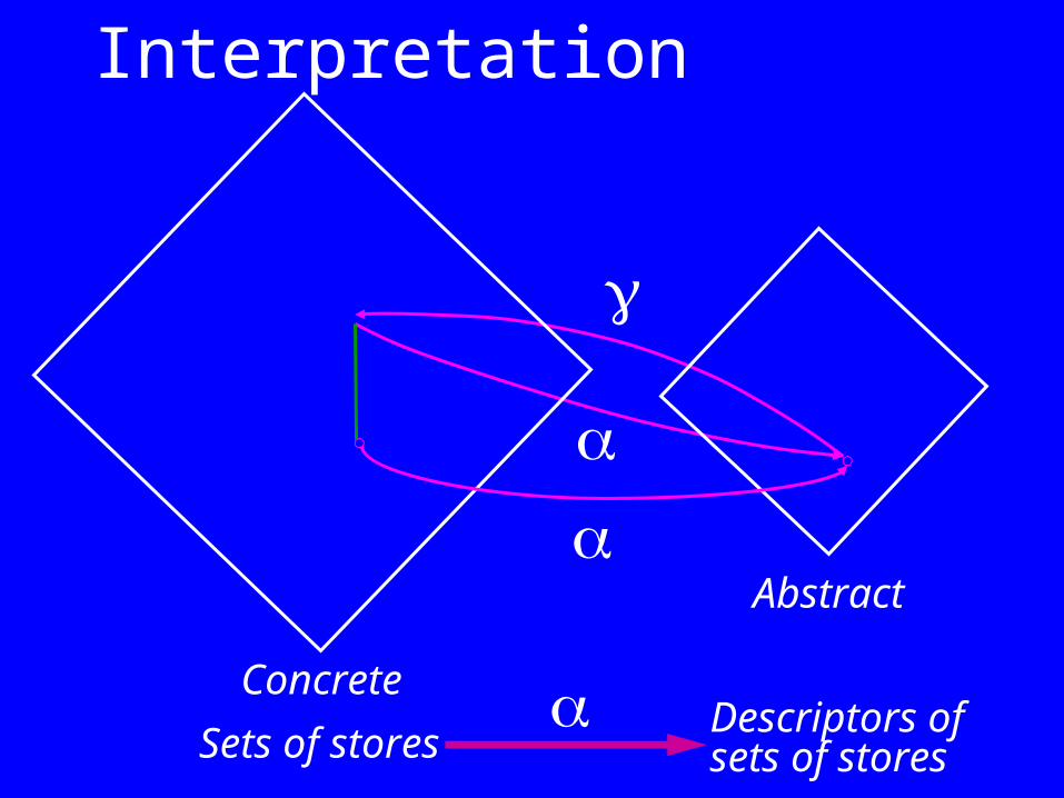
Abstract
Abstract Interpretation
Concrete
Sets of storesDescriptors ofsets of stores
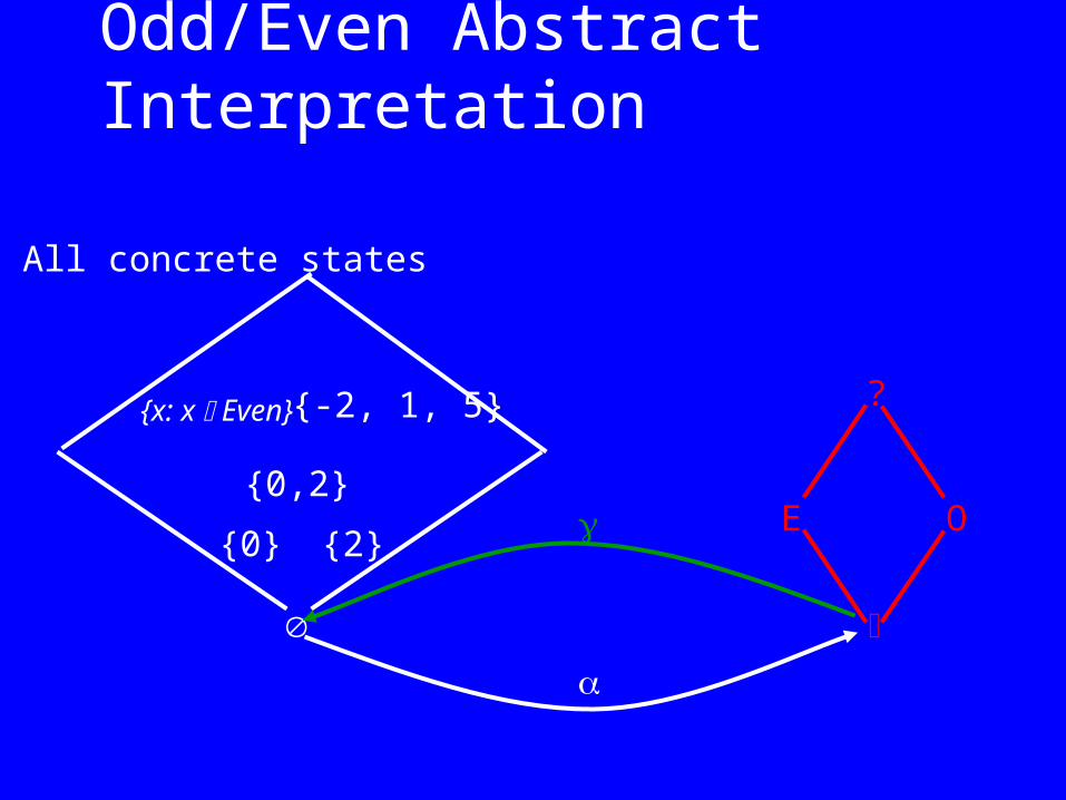
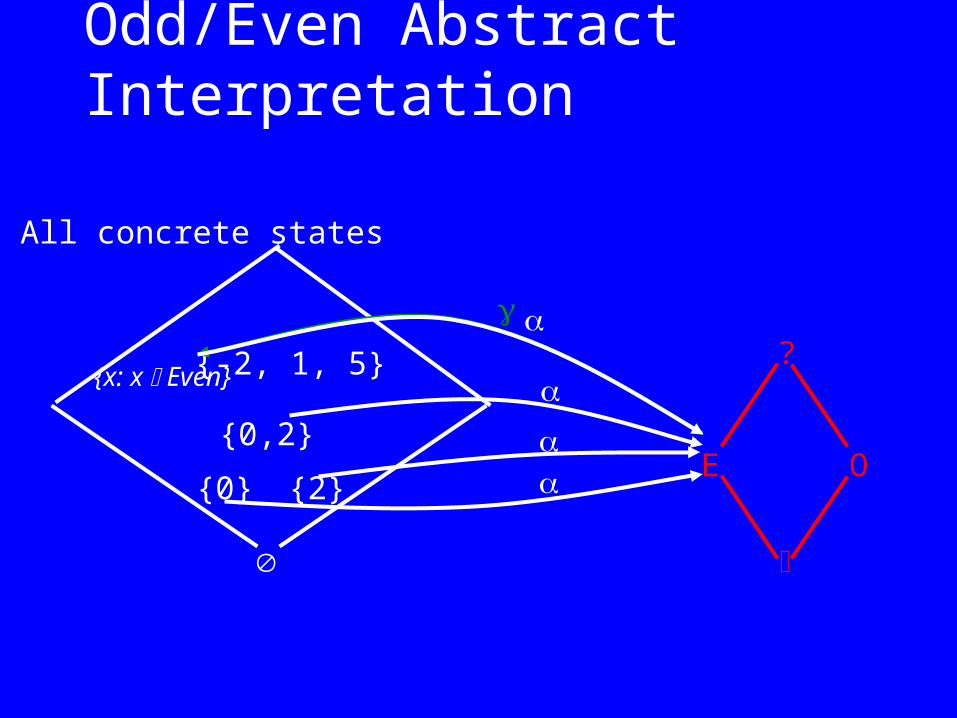
Odd/Even Abstract Interpretation
{-2, 1, 5}
{0,2}
{2}{0}
E O
?
All concrete states
{x: x Even}
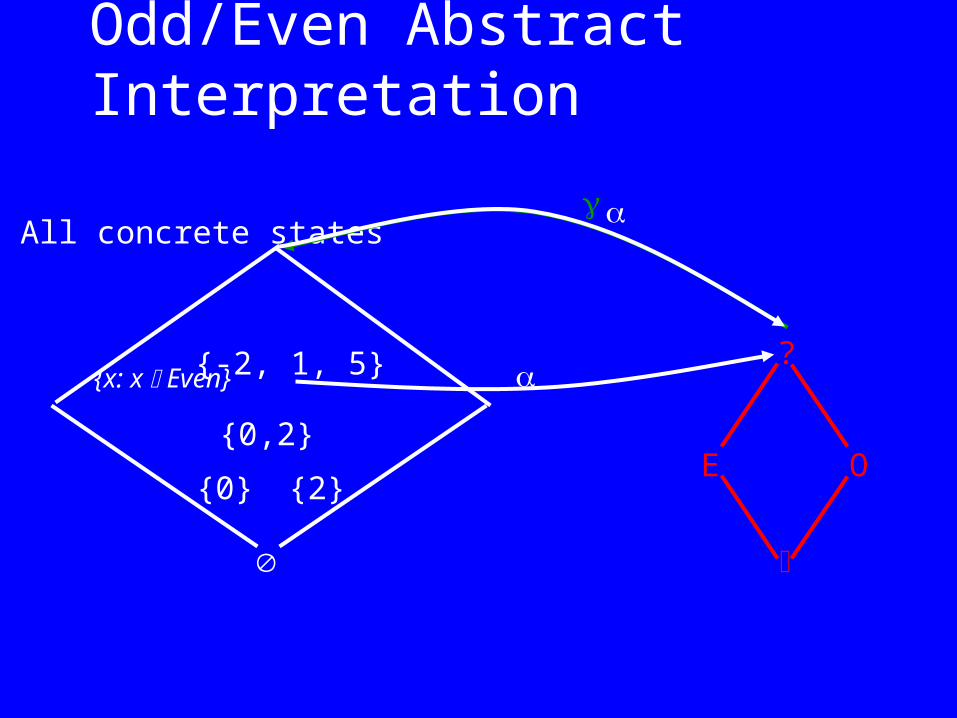
Odd/Even Abstract Interpretation
{-2, 1, 5}
{0,2}
{2}{0}
E O
?
All concrete states
{x: x Even}
Odd/Even Abstract Interpretation
{-2, 1, 5}
{0,2}
{2}{0}
E O
?
All concrete states
{x: x Even}
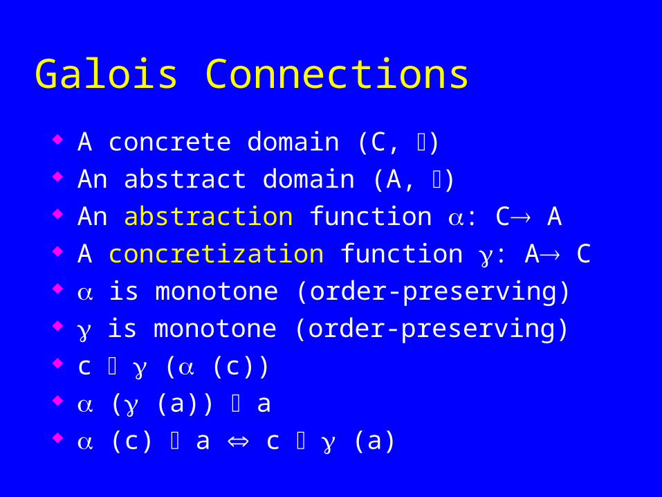
Galois Connections
A concrete domain (C, ) An abstract domain (A, ) An abstraction function : C A A concretization function : A C is monotone (order-preserving) is monotone (order-preserving) c ( (c)) ( (a)) a (c) a c (a)
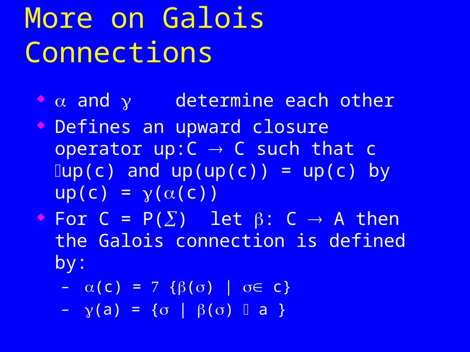
More on Galois Connections
and determine each other Defines an upward closure operator up:C C
such that c up(c) and up(up(c)) = up(c) by up(c) = ((c))
For C = P() let : C A then the Galois connection is defined by:– (c) = {() | c}
– (a) = { | () a }
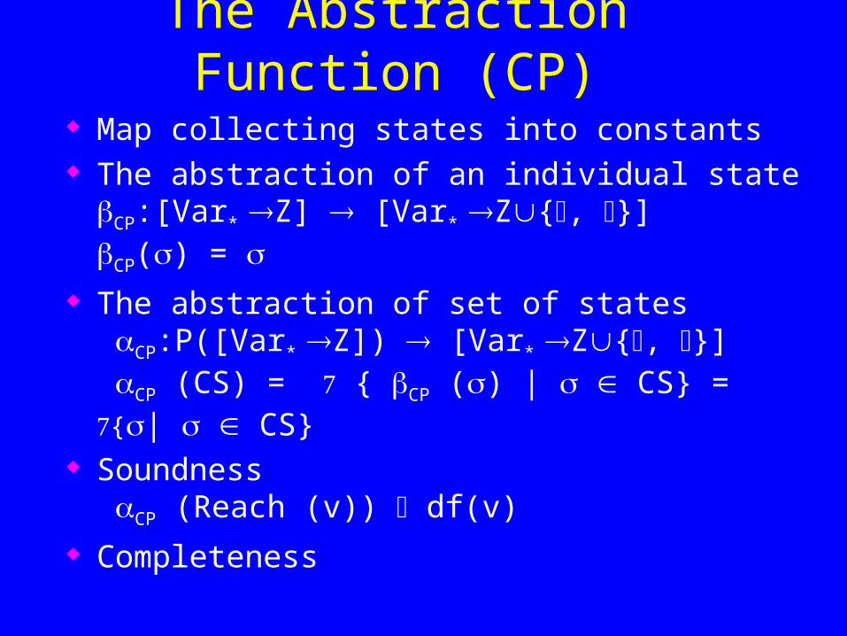
The Abstraction Function (CP) Map collecting states into constants The abstraction of an individual state
CP:[Var* Z] [Var* Z{, }]CP() =
The abstraction of set of states CP:P([Var* Z]) [Var* Z{, }] CP (CS) = { CP () | CS} = {| CS}
Soundness CP (Reach (v)) df(v)
Completeness
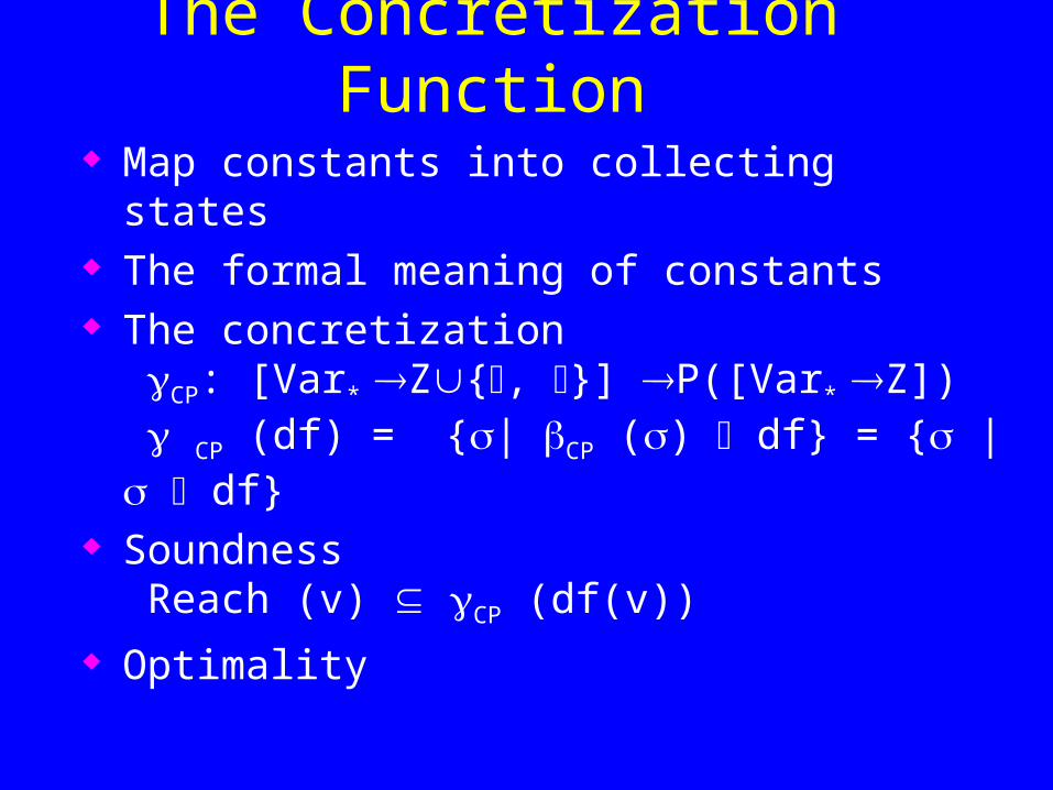
The Concretization Function Map constants into collecting states The formal meaning of constants The concretization
CP: [Var* Z{, }] P([Var* Z]) CP (df) = {| CP () df} = { | df}
Soundness Reach (v) CP (df(v))
Optimality
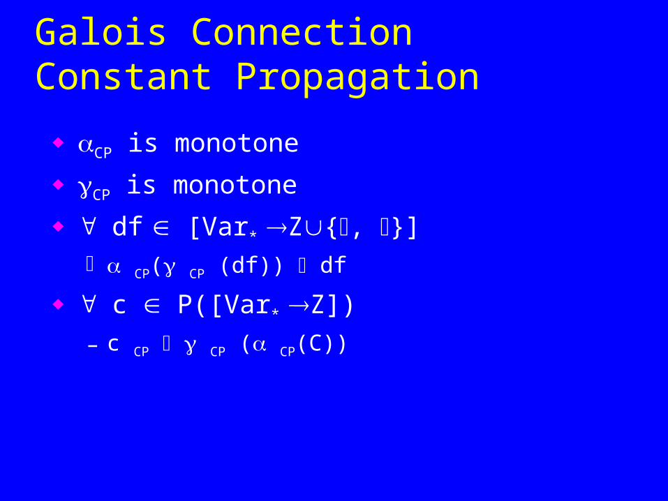
Galois Connection Constant Propagation
CP is monotone
CP is monotone
df [Var* Z{, }] CP( CP (df)) df
c P([Var* Z])
– c CP CP ( CP(C))
Upper Closure (CP)
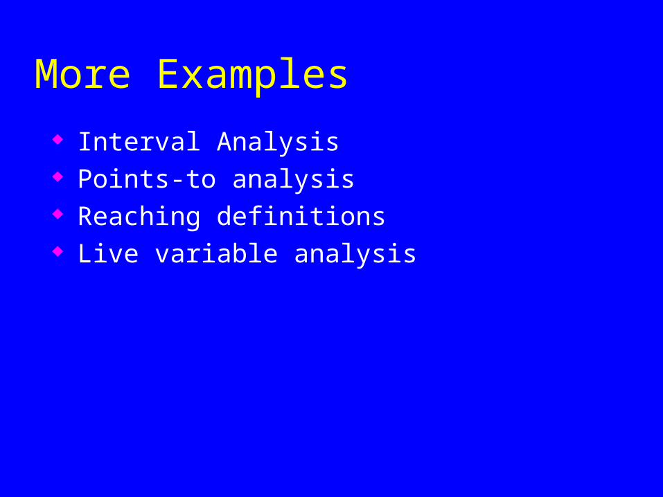
More Examples
Interval Analysis Points-to analysis Reaching definitions Live variable analysis
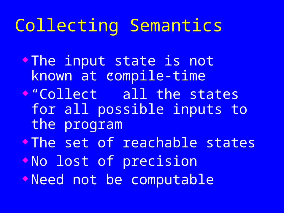
Collecting Semantics
The input state is not known at compile-time
“Collect” all the states for all possible inputs to the program
The set of reachable states No lost of precision Need not be computable
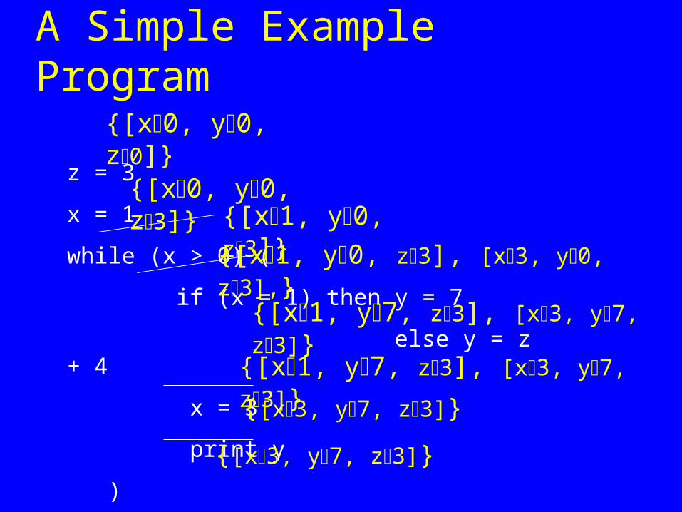
A Simple Example Program
z = 3
x = 1
while (x > 0) (
if (x = 1) then y = 7
else y = z + 4
x = 3
print y
)
{[x0, y0, z0]}
{[x1, y0, z3]}
{[x1, y0, z3], [x3, y0, z3],}
{[x0, y0, z3]}
{[x1, y7, z3], [x3, y7, z3]}
{[x1, y7, z3], [x3, y7, z3]}
{[x3, y7, z3]}
{[x3, y7, z3]}
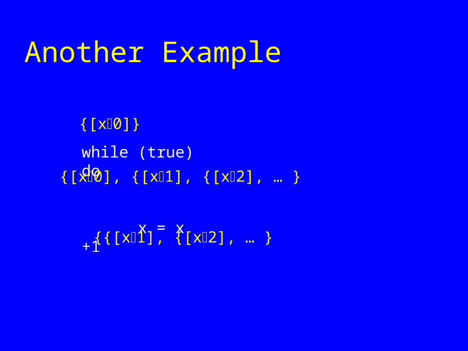
Another Example
while (true) do
x = x +1
{[x0]}
{[x0], {[x1], {[x2], … }
{{[x1], {[x2], … }
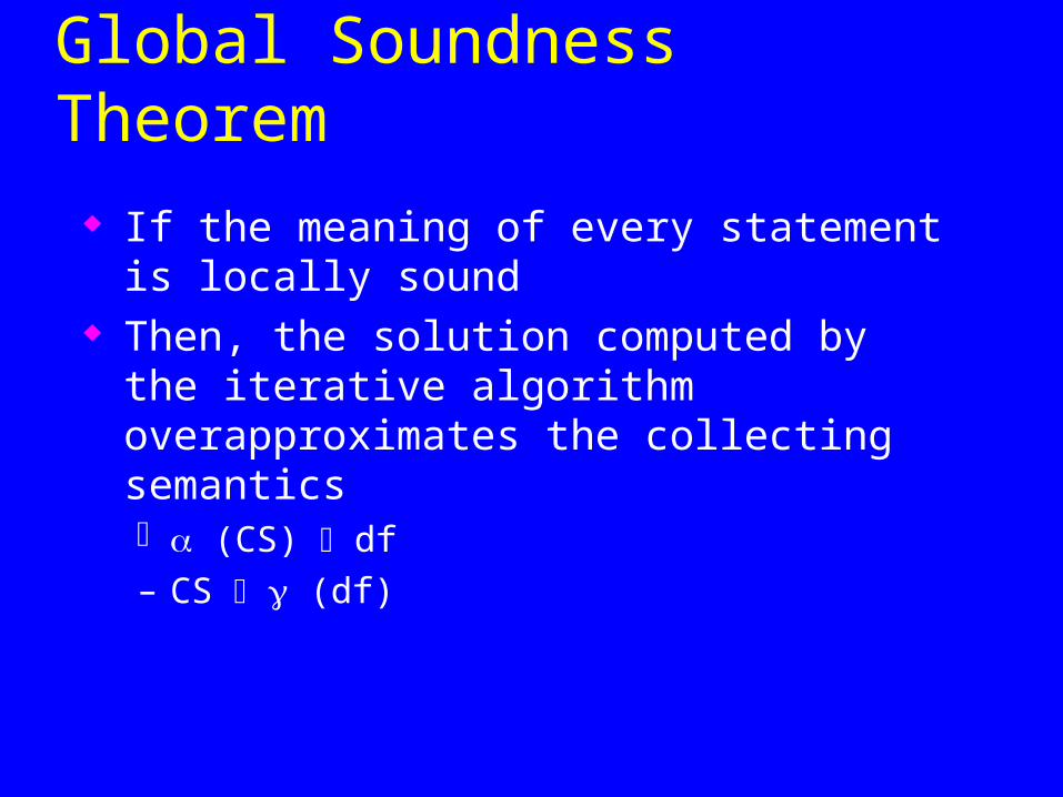
Global Soundness Theorem
If the meaning of every statement is locally sound Then, the solution computed by the iterative
algorithm overapproximates the collecting semantics (CS) df
– CS (df)
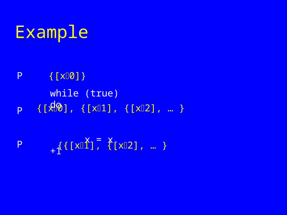
Example
while (true) do
x = x +1
{[x0]}
{[x0], {[x1], {[x2], … }
{{[x1], {[x2], … }
P
P
P
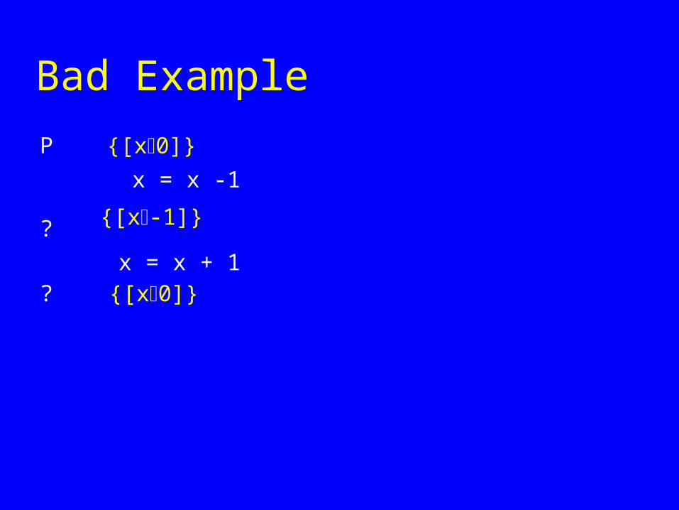
Bad Example
x = x -1
x = x + 1
{[x0]}P
?
?
{[x-1]}
{[x0]}
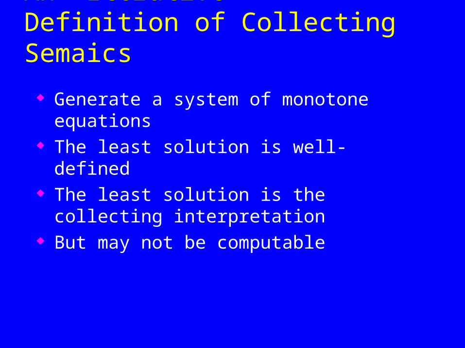
An “Iterative” Definition of Collecting Semaics
Generate a system of monotone equations The least solution is well-defined The least solution is the collecting interpretation But may not be computable
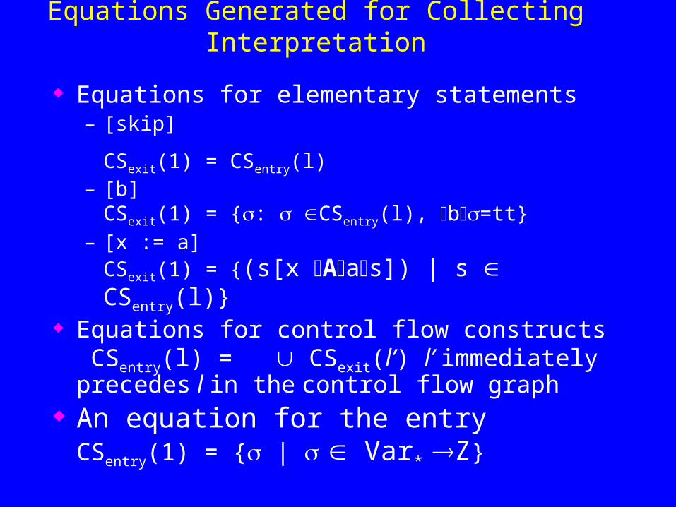
Equations Generated for Collecting Interpretation
Equations for elementary statements– [skip]
CSexit(1) = CSentry(l) – [b]
CSexit(1) = {: CSentry(l), b=tt} – [x := a]
CSexit(1) = {(s[x Aas]) | s CSentry(l)} Equations for control flow constructs
CSentry(l) = CSexit(l’) l’ immediately precedes l in the control flow graph
An equation for the entryCSentry(1) = { | Var* Z}
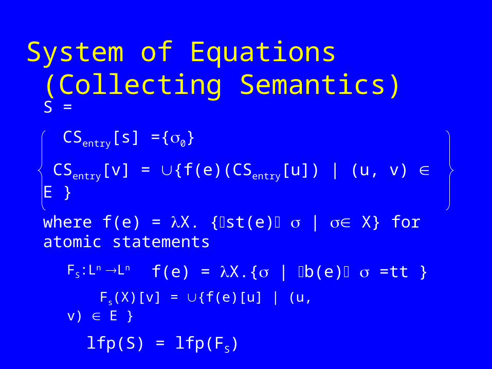
System of Equations (Collecting Semantics)
S =
CSentry[s] ={0}
CSentry[v] = {f(e)(CSentry[u]) | (u, v) E }
where f(e) = X. {st(e) | X} for atomic statements
f(e) = X.{ | b(e) =tt }
FS:Ln Ln
Fs(X)[v] = {f(e)[u] | (u, v) E }
lfp(S) = lfp(FS)
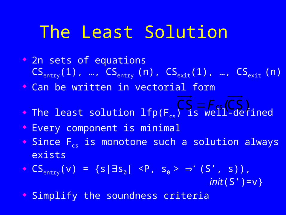
The Least Solution
2n sets of equationsCSentry(1), …, CSentry (n), CSexit(1), …, CSexit (n)
Can be written in vectorial form
The least solution lfp(Fcs) is well-defined
Every component is minimal Since Fcs is monotone such a solution always exists
CSentry(v) = {s|s0| <P, s0 > * (S’, s)), init(S’)=v}
Simplify the soundness criteria
)CS(CS csF
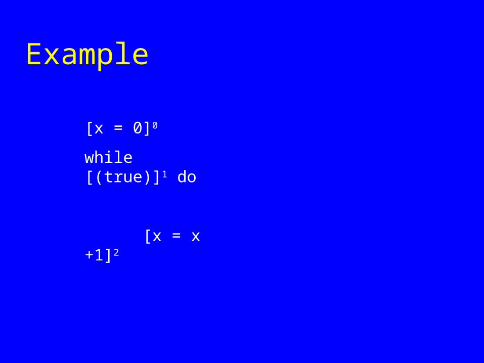
Example
[x = 0]0
while [(true)]1 do
[x = x +1]2
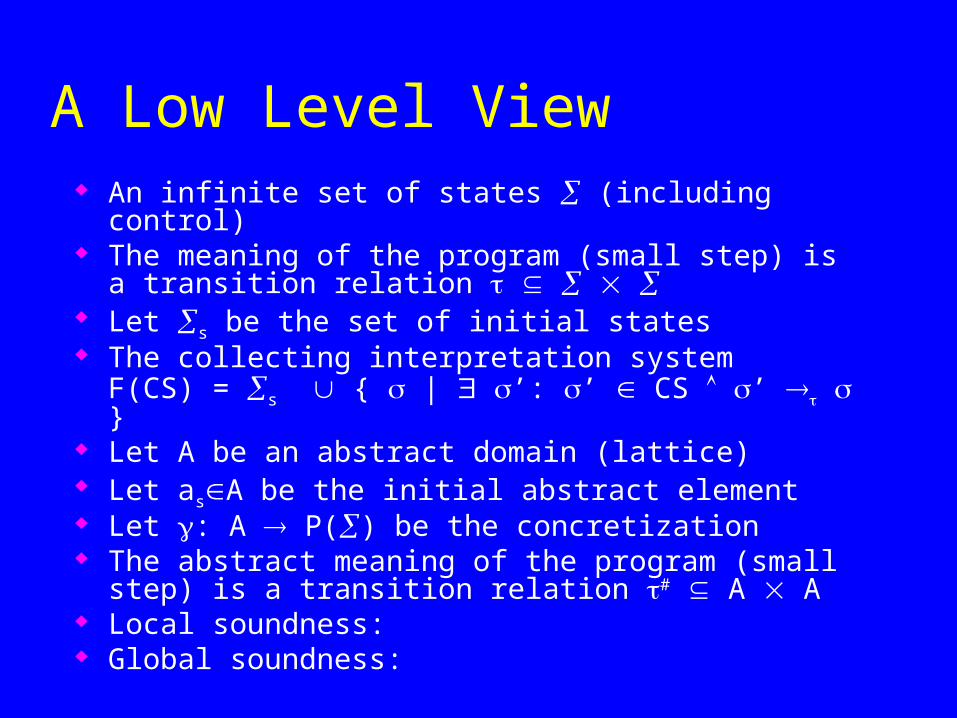
A Low Level View An infinite set of states (including control) The meaning of the program (small step) is a transition
relation Let s be the set of initial states The collecting interpretation system
F(CS) = s { | ’: ’ CS ’ } Let A be an abstract domain (lattice) Let asA be the initial abstract element Let : A P() be the concretization The abstract meaning of the program (small step) is a
transition relation # A A Local soundness: Global soundness:
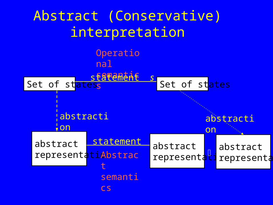
Abstract (Conservative) interpretation
abstract representation
Set of states
abstraction
Abstractsemantics
statement s abstract representation
abstraction
Operational semantics
statement sSet of states
abstract representation
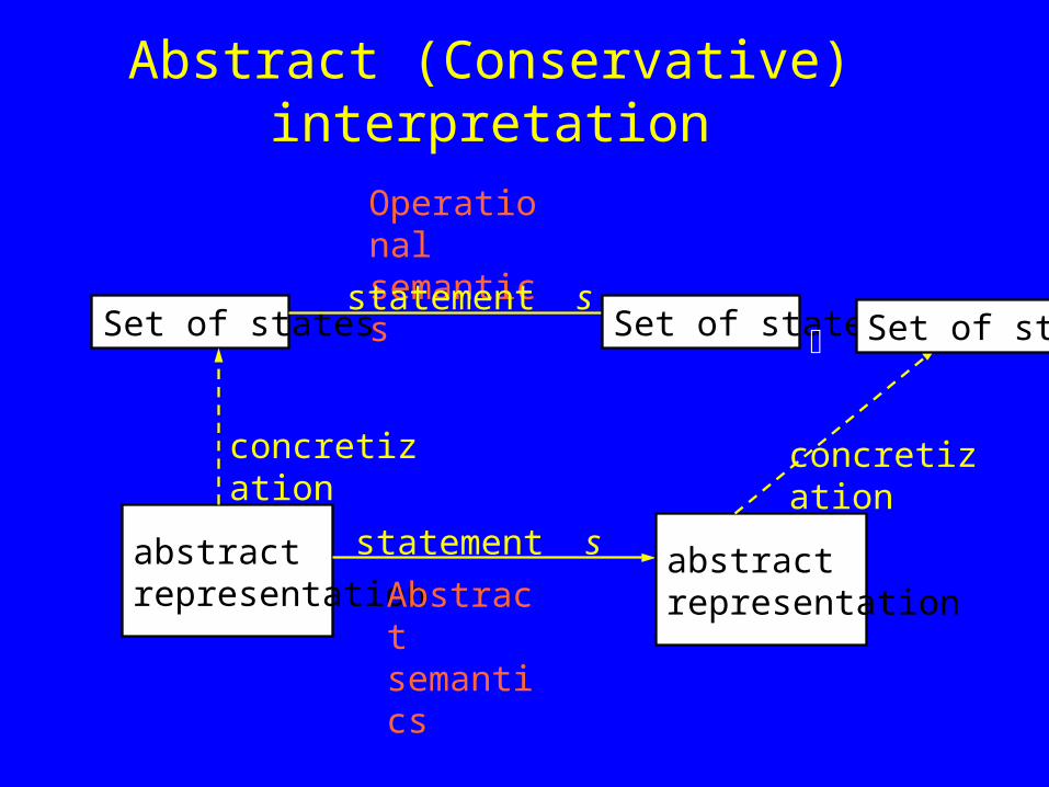
Abstract (Conservative) interpretation
abstract representation
Set of states
concretization
Abstractsemantics
statement s abstract representation
concretization
Operational semantics
statement sSet of states Set of states
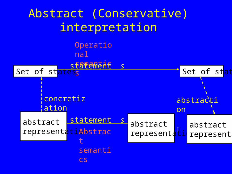
Abstract (Conservative) interpretation
abstract representation
Set of states
concretization
Abstractsemantics
statement s abstract representation
abstraction
Operational semantics
statement sSet of states
abstract representation
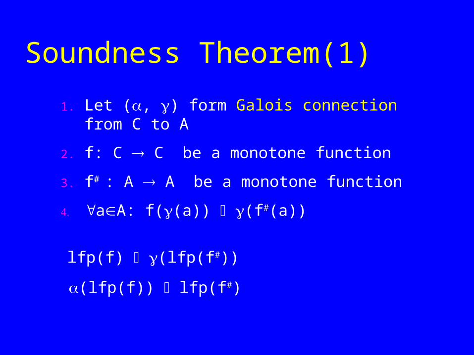
Soundness Theorem(1)
1. Let (, ) form Galois connection from C to A
2. f: C C be a monotone function
3. f# : A A be a monotone function
4. aA: f((a)) (f#(a))
lfp(f) (lfp(f#))
(lfp(f)) lfp(f#)

Soundness Theorem(2)
1. Let (, ) form Galois connection from C to A
2. f: C C be a monotone function
3. f# : A A be a monotone function
4. cC: (f(c)) f#((c))
(lfp(f)) lfp(f#)
lfp(f) (lfp(f#))

Soundness Theorem(3)
1. Let (, ) form Galois connection from C to A
2. f: C C be a monotone function
3. f# : A A be a monotone function
4. aA: (f((a))) f#(a)
(lfp(f)) lfp(f#)
lfp(f) (lfp(f#))
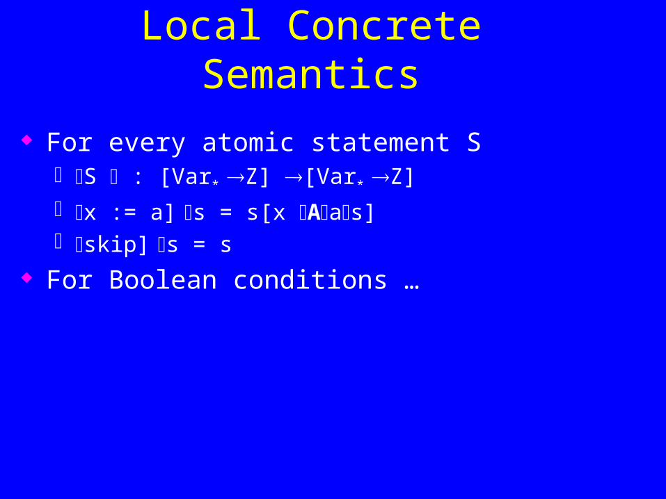
Local Concrete Semantics
For every atomic statement S S : [Var* Z] [Var* Z]
x := a] s = s[x Aas] skip] s = s
For Boolean conditions …
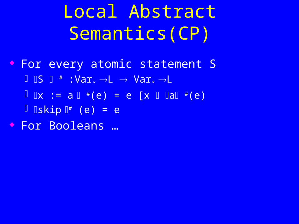
Local Abstract Semantics(CP)
For every atomic statement S S # :Var* L Var* L
x := a #(e) = e [x a #(e) skip # (e) = e
For Booleans …
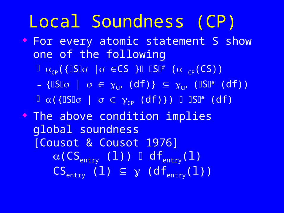
Local Soundness (CP) For every atomic statement S show one of the
following CP({S | CS } S# ( CP(CS))
– {S | CP (df)} CP (S# (df))
({S | CP (df)}) S# (df)
The above condition implies global soundness [Cousot & Cousot 1976] (CSentry (l)) dfentry(l) CSentry (l) (dfentry(l))
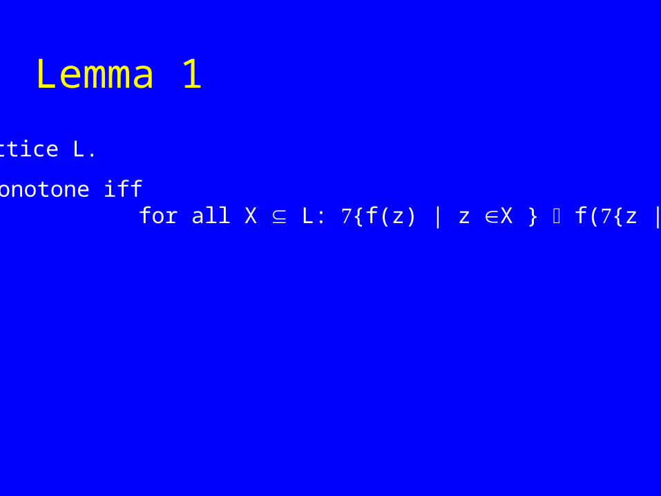
Lemma 1
Consider a lattice L.
f: L L is monotone iff for all X L: {f(z) | z X } f({z | z X })
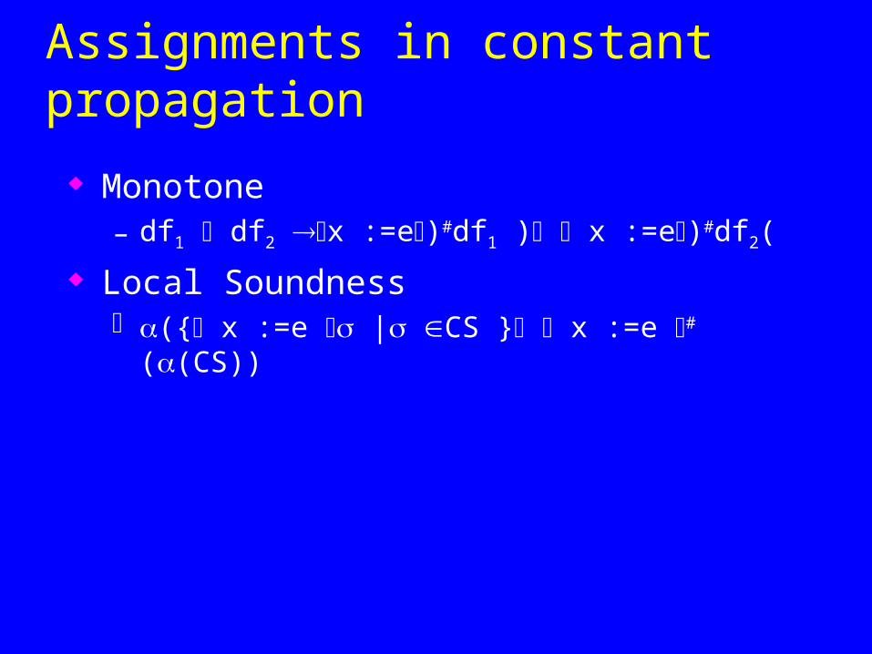
Assignments in constant propagation
Monotone– df1 df2 x :=e)#df1 ) x :=e)#df2(
Local Soundness ({ x :=e | CS } x :=e # ((CS))
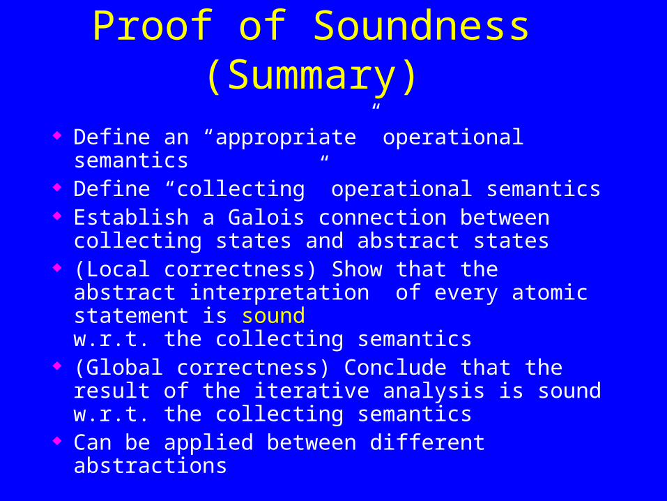
Proof of Soundness (Summary) Define an “appropriate” operational semantics Define “collecting” operational semantics Establish a Galois connection between collecting
states and abstract states (Local correctness) Show that the abstract
interpretation of every atomic statement is soundw.r.t. the collecting semantics
(Global correctness) Conclude that the result of the iterative analysis is sound w.r.t. the collecting semantics
Can be applied between different abstractions
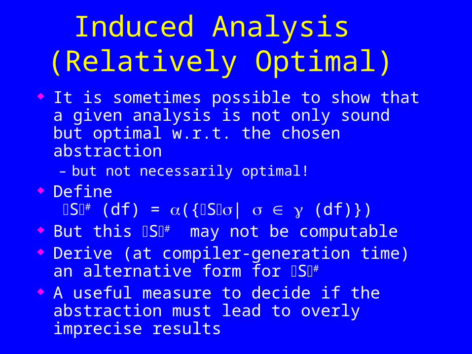
Induced Analysis (Relatively Optimal)
It is sometimes possible to show that a given analysis is not only sound but optimal w.r.t. the chosen abstraction – but not necessarily optimal!
Define S# (df) = ({S| (df)})
But this S# may not be computable Derive (at compiler-generation time) an
alternative form for S# A useful measure to decide if the abstraction must
lead to overly imprecise results
Notions of precision
CS = (df) (CS) = df Meet(Join) over all paths Using best transformers Good enough
Conclusions
Abstract interpretation relates runtime semantics and static information
The concrete semantics serves as a tool in designing abstractions
Understanding concretization is a must Understand what is preserved/lost