Abstract I. Introductionfaculty.tuck.dartmouth.edu/images/uploads/faculty/... · Canada. Phillips...
32
JOURNAL OF FINANCIAL AND QUANTITATIVE ANALYSIS Vol. 49, No. 1, Feb. 2014, pp. 1–32 COPYRIGHT 2014, MICHAEL G. FOSTER SCHOOL OF BUSINESS, UNIVERSITY OF WASHINGTON, SEATTLE, WA 98195 doi:10.1017/S0022109014000210 Real Asset Illiquidity and the Cost of Capital Hern ´ an Ortiz-Molina and Gordon M. Phillips ∗ Abstract We show that firms with more illiquid real assets have a higher cost of capital. This effect is stronger when real illiquidity arises from lower within-industry acquisition activity. Real asset illiquidity increases the cost of capital more for firms that face more competition, have less access to external capital, or are closer to default, and for those facing negative demand shocks. The effect of real asset illiquidity is distinct from that of firms’ stock illiquidity or systematic liquidity risk. These results suggest that real asset illiquidity reduces firms’ operating flexibility and through this channel their cost of capital. I. Introduction Understanding what are the sources of risk that drive firms’ cost of capital is of fundamental interest in financial economics. However, little is known about how the cost of capital may be affected by the illiquidity of a firm’s real (or phys- ical) assets. Yet, illiquidity affects a firm’s ability to redeploy its real assets to alternative uses and thus its flexibility in responding to a changing business en- vironment. For example, during June 2009 Qwest Communications solicited bids for its long-distance business, with the objectives of exiting an unprofitable busi- ness and raising cash to pay down debt. The bids came at a 50% discount from the asking price, so Qwest faced the choice of calling off the auction or accepting a large price discount. 1 ∗ Ortiz-Molina, [email protected], Sauder School of Business, University of British Columbia, 2053 Main Mall, Vancouver, BC V6T 1Z2, Canada; Phillips, gordon.phillips@marshall .usc.edu, Marshall School of Business, University of Southern California, 3670 Trousdale Pkwy, Los Angeles, CA 90089 and National Bureau of Economic Research. We thank Heitor Almeida, Hendrik Bessembinder (the editor), Murray Carlson, Jason Chen, Lorenzo Garlappi, Itay Goldstein (2009 Western Finance Association Meetings discussant), Ohad Kadan (the referee), Marcos Fabricio Perez (2010 Wilfrid Laurier Finance Conference discussant), N. R. Prabhala, Avri Ravid, Jason Schloetzer, and Laura Starks, as well as seminar participants at Georgetown University, the 2008 Pacific Northwest Finance Conference, the 2009 Western Finance Association Meetings, the 2010 Wilfrid Laurier Finance Conference, and the 2010 Northern Finance Association Meetings for their helpful comments. We also thank Pablo Mor´ an for invaluable research assistance. Ortiz-Molina acknowledges the financial support from the Social Sciences and Humanities Research Council of Canada. Phillips acknowledges support from National Science Foundation (NSF) grant 0965328. 1 See A. Sharma, “Qwest’s Long-Distance Arm Draws Bids Below Targets,” The Wall Street Journal (June 5, 2009). 1
Transcript of Abstract I. Introductionfaculty.tuck.dartmouth.edu/images/uploads/faculty/... · Canada. Phillips...

JOURNAL OF FINANCIAL AND QUANTITATIVE ANALYSIS Vol. 49, No. 1, Feb. 2014, pp. 1–32COPYRIGHT 2014, MICHAEL G. FOSTER SCHOOL OF BUSINESS, UNIVERSITY OF WASHINGTON, SEATTLE, WA 98195doi:10.1017/S0022109014000210
Real Asset Illiquidity and the Cost of Capital
Hernan Ortiz-Molina and Gordon M. Phillips∗
Abstract
We show that firms with more illiquid real assets have a higher cost of capital. This effectis stronger when real illiquidity arises from lower within-industry acquisition activity. Realasset illiquidity increases the cost of capital more for firms that face more competition, haveless access to external capital, or are closer to default, and for those facing negative demandshocks. The effect of real asset illiquidity is distinct from that of firms’ stock illiquidity orsystematic liquidity risk. These results suggest that real asset illiquidity reduces firms’operating flexibility and through this channel their cost of capital.
I. Introduction
Understanding what are the sources of risk that drive firms’ cost of capitalis of fundamental interest in financial economics. However, little is known abouthow the cost of capital may be affected by the illiquidity of a firm’s real (or phys-ical) assets. Yet, illiquidity affects a firm’s ability to redeploy its real assets toalternative uses and thus its flexibility in responding to a changing business en-vironment. For example, during June 2009 Qwest Communications solicited bidsfor its long-distance business, with the objectives of exiting an unprofitable busi-ness and raising cash to pay down debt. The bids came at a 50% discount fromthe asking price, so Qwest faced the choice of calling off the auction or acceptinga large price discount.1
∗Ortiz-Molina, [email protected], Sauder School of Business, University of BritishColumbia, 2053 Main Mall, Vancouver, BC V6T 1Z2, Canada; Phillips, [email protected], Marshall School of Business, University of Southern California, 3670 Trousdale Pkwy,Los Angeles, CA 90089 and National Bureau of Economic Research. We thank Heitor Almeida,Hendrik Bessembinder (the editor), Murray Carlson, Jason Chen, Lorenzo Garlappi, Itay Goldstein(2009 Western Finance Association Meetings discussant), Ohad Kadan (the referee), MarcosFabricio Perez (2010 Wilfrid Laurier Finance Conference discussant), N. R. Prabhala, Avri Ravid,Jason Schloetzer, and Laura Starks, as well as seminar participants at Georgetown University, the2008 Pacific Northwest Finance Conference, the 2009 Western Finance Association Meetings, the2010 Wilfrid Laurier Finance Conference, and the 2010 Northern Finance Association Meetings fortheir helpful comments. We also thank Pablo Moran for invaluable research assistance. Ortiz-Molinaacknowledges the financial support from the Social Sciences and Humanities Research Council ofCanada. Phillips acknowledges support from National Science Foundation (NSF) grant 0965328.
1See A. Sharma, “Qwest’s Long-Distance Arm Draws Bids Below Targets,” The Wall StreetJournal (June 5, 2009).
1

2 Journal of Financial and Quantitative Analysis
In this paper, we argue that real asset illiquidity reduces firms’ operating flex-ibility and is thus an economically important source of equity risk. Our study ismotivated by the observation that sales of real assets in illiquid markets fetch largeprice discounts relative to their fundamental values (e.g., Pulvino (1998), Rameyand Shapiro (2001), and Gavazza (2011)), which increases firms’ cost of unwind-ing their capital stock and reduces their ability to raise cash with asset sales. Sinceasset sales are central to firms’ restructuring processes (Maksimovic and Phillips(1998)) and are affected by the illiquidity of real asset markets (Schlingemann,Stulz, and Walkling (2002)), real asset illiquidity might increase equity risk.
Real asset illiquidity is especially harmful in bad times, when firms are underpressure to restructure their operations and maneuver to avoid default. In partic-ular, real asset illiquidity can induce firms facing economic adversity to remainburdened with unproductive assets, which often generate large fixed costs. The re-sulting operating leverage increases the covariance of a firm’s performance withmacroeconomic conditions, especially during downturns, leading to a higher costof capital. Hence, we examine whether, by reducing firms’ operating flexibility,real asset illiquidity increases their cost of capital, in particular during downturns.
Our key dependent variable is the implied cost of capital (ICC), which doesnot rely on noisy realized returns or specific asset pricing models, and whichPastor, Sinha, and Swaminathan (2008) show is a good proxy for a stock’s condi-tional expected return. Elton (1999) argues against using realized returns in assetpricing tests and highlights that the relation between realized returns and risk canbe negative for long periods. Lundblad (2007) shows that a very long sample isneeded to detect a positive risk-return relation using realized returns. In contrast,the ICC detects a positive intertemporal risk-return tradeoff (Pastor et al. (2008))and a positive relation between distress risk and expected returns (Chava andPurnanandam (2010)).2 For robustness, we also measure expected returns usingFama and French’s (1993) 3-factor model cost of capital (FFCC), but this measureis imprecise (Fama and French (1997), Pastor and Stambaugh (1999)).
We use asset illiquidity measures that capture the illiquidity of real (fixed) as-sets at the industry level and of balance-sheet measures that capture the illiquidityof total assets at the firm level. The industry-level measures of real asset illiquidityare motivated by Almeida, Campello, and Hackbarth (2011) and Schlingemannet al. (2002). They reflect the “industry equilibrium” aspect of real asset illiquid-ity stressed by Shleifer and Vishny (1992), that is, a firm can more easily sellits industry-specific assets to other firms in the industry with financial slack. Thefirm-level measures of total asset illiquidity assign illiquidity scores to each assetclass in a firm’s balance sheet and capture the differential illiquidity of the dif-ferent types (or composition) of assets a firm holds as in Berger and Bouwman(2009) and Gopalan, Kadan, and Pevzner (2012).
We show that real asset illiquidity is a major source of operating inflexibil-ity, and that it has an economically significant impact on a firm’s cost of capital.In univariate tests using both the ICC and the FFCC and the measures of realasset illiquidity, we find a real asset illiquidity premium (i.e., the cost of capital
2In an international setting, Lee, Ng, and Swaminathan (2009) further show that the ICC providesclear evidence of economic relations that would otherwise be obscured by the noise in realized returns.

Ortiz-Molina and Phillips 3
is higher for firms in the highest vs. the lowest real asset illiquidity quintiles).Supporting the view that operating inflexibility causes time-varying equity risk,the illiquidity premium is countercyclical, which suggests it is driven by costlyreversibility of investment. Our multivariate cross-sectional and time-series testsfurther support our hypothesis: Firms with more illiquid real assets have highercost of capital than firms with less illiquid real assets, and firms’ cost of capi-tal is higher during periods of high real asset illiquidity. These tests imply thata 1-standard-deviation increase in real asset illiquidity across firms increases theICC by 0.9 to 1.4 percentage points and that a similar increase over time increasesit by 0.5 to 1.4 percentage points. We further show that the balance-sheet measuresof total asset illiquidity at the firm level also have a positive impact on the ICC,and that this impact is largely driven by firms’ cash holdings. This evidence sug-gests that the illiquidity of both real and total assets are important determinants offirms’ flexibility and thus of their cost of capital.
Our results are robust to the worry that the ICC might measure expectedreturns with systematic error due to either biases or sluggish revisions in the an-alyst earnings forecasts used to calculate it. Our results are similar if we use anICC corrected for the sluggishness of analyst earnings forecast revisions as sug-gested by Guay, Kothari, and Shu (2011) and if we restrict attention to firms withsmall analyst earnings forecast errors. They are also similar if we discard the pos-sibly more noisy estimates of the cost of capital, which are below the risk-freerate.
We also distinguish between “inside” real asset illiquidity (provided by ac-quirers of assets that operate in the industry) and “outside” real asset illiquidity(provided by acquirers of assets that operate outside the industry). Buyers frominside the industry can better redeploy the asset to a productive use and are willingto pay higher prices (Shleifer and Vishny (1992)). Hence, less mergers and acqui-sitions (M&A) activity by industry insiders should make real asset markets moreilliquid than less M&A activity by industry outsiders. Supporting this view, wefind that inside illiquidity increases firms’ ICC by more than outside illiquidity.This result is in line with that in Almeida et al. (2011), who find that distressedfirms with industry-specific assets can often sell them to financially flexible in-dustry insiders rather than to industry outsiders.
The effect of real asset illiquidity on the cost of capital varies across firms inways that are broadly consistent with the operating inflexibility channel. Specifi-cally, the effect is larger when the cost of inflexible operations due to illiquid assetmarkets is arguably higher. First, it is larger for firms that face more competitiverisk in product markets, that is, for firms in low-concentration (more competitive)industries and for the smaller firms within the industry. Second, it is larger forfirms that have less access to external capital or are closer to default. Last, it islarger for firms facing negative demand shocks (i.e., for firms with low valuationsor in industry downturns).
Our main results hold after controlling for firm value, growth options, andasset specificities. We further show that the effect of real asset illiquidity on thecost of capital is robust to controlling for the illiquidity and systematic liquid-ity risk of firms’ stocks. In addition, we show that real asset illiquidity increasesthe ICC after controlling for the industry’s valuation. This shows that our results
4 Journal of Financial and Quantitative Analysis
are not biased by a correlation between our measures of real asset illiquidity andchanges in industry valuation or the supply of capital. Moreover, our results holdif we measure expected returns using the unlevered implied cost of capital, andif we do the tests using industry averages of the variables. In addition, real assetilliquidity reduces firm value after controlling for cash flow effects, further sug-gesting that it affects firms’ discount rates. Lastly, our results also hold if we usebusiness segment-weighted measures of real asset illiquidity.
Our paper is related to early work that suggests that operating inflexibilityincreases the systematic risk of a firm’s equity, such as Rubinstein (1973), Lev(1974), Mandelker and Rhee (1984), and Booth (1991), who show that operat-ing leverage increases expected returns in the capital asset pricing model. Wecontribute to these studies by identifying real asset illiquidity as a key source ofoperating leverage and showing that it impacts the cost of capital.
Our evidence complements that of Benmelech and Bergman (2009), whohighlight the role of real asset illiquidity in debt markets. They find that debttranches of airlines secured with more redeployable collateral have higher ratingsand lower yield spreads. Hence, the evidence from our study and theirs suggeststhat real asset illiquidity increases a firm’s overall cost of capital.
Also related is the recent investment-based asset pricing literature thatargues that differences in operating flexibility across value and growth firms canexplain the value premium (e.g., Kogan (2004), Gomes, Kogan, and Zhang (2003),Carlson, Fisher, and Giammarino (2004), Zhang (2005), and Cooper (2006)). Weadd to this work by showing that real asset illiquidity, which directly reduces op-erating flexibility, significantly increases a firm’s cost of equity.
Last, our work adds to the literature on what determines the implied costof capital, such as earnings attributes (Francis, LaFond, Olsson, and Schipper(2004)), institutions and securities regulation (Hail and Leuz (2006)), leverageand taxes (Dhaliwal, Heitzman, and Li (2006)), cross-listing (Hail and Leuz(2009)), governance and country-level investor protection (Chen, Chen, and Wei(2009)), default risk (Chava and Purnanandam (2010)), shareholder rights(Chen, Chen, and Wei (2011)), and labor unionization (Chen, Kacperczyk, andOrtiz-Molina (2011)).
The paper is structured as follows: Section II develops our main hypothesisand related predictions. Section III describes our data and variables. Section IVreports the main empirical results. Section V studies the cross-sectional variationin the effect of real asset illiquidity on the cost of capital. Section VI presentsseveral robustness tests. Section VII concludes.
II. Illiquid Real Assets and the Cost of Capital
Our conceptual framework is based on the corporate finance literature, whichhighlights the role of asset sales in firms’ responses to changing economic condi-tions as well as on the asset pricing literature, which relates operating flexibility toequity risk. Sales of real assets in illiquid markets fetch large price discounts (e.g.,Pulvino (1998)), which increases a firm’s cost of reversing investment and reducesits ability to raise cash. Hence, real asset illiquidity makes firms’ restructuring pro-cesses more difficult (e.g., Maksimovic and Phillips (1998)), which is especially

Ortiz-Molina and Phillips 5
costly to firms facing economic adversity (e.g., Lang, Poulsen, and Stulz (1995)).Such firms find it difficult to scale down operations and raise cash, and thus of-ten remain burdened with unproductive assets. This increases the covariance of afirm’s performance with macroeconomic conditions, especially during downturns.It is noteworthy that, in addition to reducing firms’ ability to raise cash, illiquidreal assets generate long-term obligations (e.g., fixed operating costs, wage con-tracts, and commitments to suppliers), and prior work (e.g., Lev (1974)) showsthat operating leverage increases the cost of capital.3
This leads to our main hypothesis: Real asset illiquidity increases firms’ costof capital by decreasing their operating flexibility.
Our main hypothesis has three broad implications. The first implicationshould hold at the aggregate level. Specifically, there should be a positive spreadin cost of capital between the high and low real asset illiquidity firms, that is,a real asset illiquidity premium. Moreover, real asset illiquidity is more harmfulwhen economic conditions worsen and firms are more likely to need to sell assets,either to reduce fixed costs and thus operating risk or to raise the cash necessaryto fund operations and avoid default. In sum, there should be a countercyclicalaggregate real asset illiquidity premium. The second implication follows directlyfrom the hypothesis: In firm-level multivariate tests, there should be a positiveimpact of real asset illiquidity on the cost of capital.
The third implication follows from Shleifer and Vishny (1992). They arguethat buyers who operate outside the industry are willing to pay low prices due tolittle synergies and inexperience in operating the asset, while buyers who oper-ate inside the industry can better redeploy the asset to productive uses and thusare willing to pay high prices. Supporting this view, financially constrained firmsforced to sell assets to industry outsiders obtain much lower prices than those theywould have obtained from industry insiders (e.g., Pulvino (1998)). This suggeststhat a weaker presence of inside buyers makes real asset markets more illiquidthan a weaker presence of outside buyers and thus should have a stronger positiveeffect on firms’ cost of capital.
We also develop predictions about what drives the variation across firms inthe effect of real asset illiquidity. We first consider the role of a firm’s competitiveenvironment. Real asset illiquidity is likely to be more costly for firms in morecompetitive industries, where competition is more intense and thus firms that failto quickly adapt to changes in the environment are drawn out of business.4 It isalso likely to be more costly for the smallest industry competitors, which are lessable to endure economic hardship and are often exposed to competitive threatsfrom larger rivals.5 These arguments suggest that real asset illiquidity should
3In the same vein, the recent investment-based asset pricing literature, which aims to explainthe value anomaly (e.g., Carlson et al. (2004)), argues that the returns of firms with more operatinginflexibility load more on the state of the economy, which leads investors to require higher expectedreturns for their capital.
4Hou and Robinson (2006) empirically show that the stocks of firms operating in more competitiveindustries earn higher average returns and attribute this to their higher default risk.
5Smaller stocks are arguably more risky due to their higher distress risk (e.g., Chan and Chen(1991)), and the empirical evidence shows that small firms account for the majority of exits in industryrestructurings.

6 Journal of Financial and Quantitative Analysis
increase the cost of capital more for firms in more competitive industries andfor the smallest firms in each industry.
We then consider the role of a firm’s access to capital and financial condition.Real asset illiquidity is likely to be more costly for firms with less access to ex-ternal capital and for firms that are closer to financial distress, since such firmsmay be forced to raise cash with asset sales. Supporting the view, Campello,Graham, and Harvey (2010) report that during the recent financial crisis finan-cially constrained firms have engaged in significantly more asset sales than haveunconstrained firms. This suggests that real asset illiquidity should increase thecost of capital more for firms with less access to capital and for those with moredefault risk.
Last, we consider the role of a firm’s business environment. Theory suggeststhat a firm’s ability to sell its real assets is more valuable in bad times, when firmsfacing a low demand for their products may want to sell real assets to reduce theirfixed costs or to raise cash (e.g., Kogan (2001), Zhang (2005)). This suggests thatreal asset illiquidity should increase the cost of capital more for firms with lowvaluations and for those in industries experiencing downturns.
These testable implications are summarized below:
Prediction 1. At the aggregate level, there should be a real asset illiquidity pre-mium in the cost of capital that exhibits a countercyclical time-series variation.
Prediction 2. Firms with more illiquid real assets should have a higher cost ofcapital.
Prediction 3. Inside real asset illiquidity should increase a firm’s cost of capitalmore than outside real asset illiquidity.
Prediction 4. Real asset illiquidity should increase the cost of capital more for:
i) firms in more competitive industries and the smallest firms in each industry,
ii) firms with less access to capital and firms with higher default risk, and
iii) firms with lower valuations and firms in industries experiencing downturns.
III. Data and Variables
A. Data Sources and Sample Selection
Our data come from the Center for Research in Security Prices (CRSP)-Compustat Merged Database, the Compustat Segment Database, the InstitutionalBrokers’ Estimate System (IBES), the Securities Data Corporation (SDC), theSt. Louis Federal Reserve Economic Data (FRED), and the Census of Manufac-tures. We start with the CRSP-Compustat Merged Database and exclude compa-nies in the financial (Standard Industrial Classification (SIC) codes 6000–6999)and utilities (SIC codes 4900–4999) industries. We also drop companies notcovered in IBES because we require analyst forecast data to calculate the im-plied cost of capital, and observations for which we are unable to compute thereal asset illiquidity measures or our control variables. Our final sample includes

Ortiz-Molina and Phillips 7
6,260 firms operating in 304 different 3-digit SIC industries and 33,788 firm-yearobservations during 1984–2006.
B. Measures of Asset Illiquidity
Given our conceptual framework, our main explanatory variables are realasset illiquidity measures, which capture only the illiquidity of fixed assets anda firm’s ability to resell these assets to other firms in the industry. We also ex-amine the effect of total asset illiquidity measures constructed at the firm levelfrom firms’ balance sheets, which capture not only the illiquidity of fixed as-sets but also the effect of how much cash or other liquid assets the firmholds.
1. Illiquidity of Firms’ Real Assets
The measures of real asset illiquidity capture the “industry equilibrium” as-pect of asset illiquidity highlighted by Shleifer and Vishny (1992), that is, the factthat the liquidity of a firm’s fixed assets is intimately related to the presence andfinancial ability of other firms in the industry (the natural buyers) to act as acquir-ers. More recently, Gavazza (2011) and Benmelech and Bergman (2008), (2009)all highlight the importance of the set of potential buyers from within the indus-try in determining real asset liquidity. An additional advantage of the measuresis that they are more likely to be exogenous to the firm and mitigate potentialendogeneity concerns.
The liquidity of a firm’s real assets (the extent to which the asset can bequickly sold at a fair price) depends on the existence of other firms with enoughfinancial slack to purchase it and the extent to which the asset is transferrable toother firms. The existence of other firms with financial slack can be gauged em-pirically, but measuring the degree of asset specificity, and thus the transferabilityof assets across firms, is much more difficult. Still, the key source of asset speci-ficity is the firm’s industry affiliation (e.g., Kogan (2004)). Due to commonalitiesin production technologies, most assets are transferrable among firms in the sameindustry but much harder to transfer to firms outside the industry. Supporting thisview, the bulk of asset sales occur between firms in the same or closely relatedindustries (Maksimovic and Phillips (2001)).
We use three measures of real asset illiquidity based on industry definitions atthe 3-digit SIC level. The first two capture the absence of potential future buyersfrom within the industry and are motivated by Shleifer and Vishny (1992) andAlmeida et al. (2011). They assume that a firm’s assets are transferrable to otherfirms in the industry, which are able to redeploy them to alternative uses, but nottransferrable to firms outside the industry (i.e., they are industry specific).6 Hence,financially flexible industry insiders are the likely future buyers of a firm’s assets.Thus, a firm’s real assets are more illiquid when the number of potential inside-industry buyers with financial slack is smaller.
6There might also be some heterogeneity in the transferability of assets across firms within theindustry. Hence, in our tests we also include firm-level control variables, which capture the degree ofspecificity of each firm’s assets.

8 Journal of Financial and Quantitative Analysis
Our first measure is similar to those used in Benmelech and Bergman (2008),(2009) and Gavazza (2011) for the airline industry.7 This measure is minus thenumber of potential buyers for a firm’s assets, MNoPotBuy, defined for each firmas minus the number of rival firms in the industry that have debt ratings.
Our second measure, denoted NLPotBuy, directly captures the financial slackof potential buyers, and for each firm it is defined as the average book leverage netof cash of rival firms in the industry, averaged over the last 5 years to minimize theimpact of temporary changes in firms’ financial situations. A firm’s real assets aremore illiquid for higher values of both MNoPotBuy and NLPotBuy. These mea-sures have an important industry component (we identify rivals using SIC codes),but they vary across firms in the same industry.
Our third measure, MTotM&A, follows Schlingemann et al. (2002). It cap-tures the historical illiquidity of a firm’s assets using minus the value of M&Aactivity in the firm’s industry scaled by industry assets (Sibilkov (2009) uses asimilar measure). We obtain the value of all M&A deals involving publicly tradedtargets in each 3-digit SIC industry and year from SDC.8 We include both mergersand acquisitions of assets (the latter comprise 75% of the deals). In industry-yearswith no reported transactions, we set the value equal to 0. We then multiply thevalue of transactions in the industry by −1, scale it by the book value of as-sets in the industry, and average this ratio over the past 5 years.9 The last stepsmoothes temporary ups and downs in M&A activity to better capture the in-trinsic salability of an industry’s assets. Higher values of MTotM&A imply moreilliquid real assets. This measure captures the salability of assets, regardless ofwhether it is driven by the presence of solvent rivals or by the asset’s transferabil-ity. It uses transactions involving buyers both from inside and outside the industry,and thus it does not rely on assumptions about the transferability of assets acrossindustries.
We decompose MTotM&A to discern between weaker acquisition activity byindustry insiders (those who operate in the same 3-digit SIC industry as the target)and by industry outsiders (those who do not operate in the industry). We classifya purchase as made by an industry insider if the buyer has any segments in thesame industry as the assets purchased, checking over each reported industry ofthe target if it reports multiple industries. MInM&A is minus the value of M&Aactivity in the industry involving acquirers that operate within the industry, scaledby the book value of the assets in the industry. MOutM&A is minus the value ofM&A activity in the industry involving acquirers that operate outside the industry,scaled by the book value of the assets in the industry. Both of these variables areaveraged over the past 5 years.
7They develop measures of illiquidity based on the idea that the potential secondary market buyersfor any given type of aircraft are likely to be financially healthy airlines already operating the sametype of aircraft.
8We focus on publicly traded targets because the Compustat firms for which we wish to measurereal asset illiquidity are publicly traded, and because acquisitions of private targets are likely to bereported with significant noise.
9We calculate the value of assets in an industry by summing the assets in the industry of single-segment firms and the segment-level assets of multisegment firms, breaking up multisegment firmsinto their component industries.

Ortiz-Molina and Phillips 9
2. Overall Asset Illiquidity
As in Gopalan et al. (2012), we construct four firm-level weighted measuresof total asset illiquidity. These measures sum the liquidity scores assigned toeach of the major asset classes in a firm’s balance sheet (holdings of cash andequivalents, other noncash current assets, tangible fixed assets, and other assets)weighted by the importance of each asset class in the total assets of the firm (alsosee Berger and Bouwman (2009) for a similar approach). We only differ in thatwe multiply each measure by −1, so that we can interpret it as an asset illiquiditymeasure. The resulting weighted asset illiquidity measures are described below,where all measures of total assets and market assets in the denominator are lagged1 year:
WAIL1 = −(
Cash & EquivTotal Assets
),
WAIL2 = −[(
Cash & EquivTotal Assets
)+ 0.5
(Noncash CATotal Assets
)],
WAIL3 = −[(
Cash & EquivTotal Assets
)+ 0.75
(Noncash CATotal Assets
)
+ 0.5
(Tangible Fixed Assets
Total Assets
)],
MWAIL = −[(
Cash & EquivMarket Assets
)+ 0.75
(Noncash CA
Market Assets
)
+ 0.5
(Tangible Fixed Assets
Market Assets
)].
C. Measures of Cost of Capital
We use two ex ante measures of a firm’s expected return. Our main measureis the implied cost of capital (ICC), which does not rely on noisy realized returnsor on specific asset pricing models. Pastor et al. (2008) theoretically show that ICCis a good proxy for expected returns and that, unlike realized returns, it empiri-cally identifies a positive risk-return tradeoff (see also Chava and Purnanandam(2010)). Sluggish adjustment or biases in analyst earnings forecasts might affectthe ICC (Easton and Monahan (2005) and Guay et al. (2011)), but in Section IV.Dwe show that these issues do not drive our results. For robustness, we also use theFama and French (1993) 3-factor model cost of capital (FFCC), but this measureis very imprecise (Fama and French (1997), Pastor and Stambaugh (1999)).
Following Gebhardt, Lee, and Swaminathan (2001), the ICC is defined asthe discount rate that equates the present value of all expected future cash flowsto shareholders to the current stock price. The calculation of a firm’s ICC for yeart starts with the dividend-discount model:
Pt =
∞∑i=1
Et(Dt+i)
(1 + re)i,(1)

10 Journal of Financial and Quantitative Analysis
where P is the stock price, D is dividends, re is the discount rate, and E(·) is theexpectation operator. Assuming clean-surplus accounting (change in book equityequals net income minus dividends) and using equation (1), we get the discountedresidual income equity valuation model:
Pt = Bt +∞∑
i=1
Et[(ROEt+i − re)Bt+i−1]
(1 + re)i,(2)
where ROE is the return on equity and B is the book value of equity. We thennumerically solve for the implied cost of equity, re, from equation (2) using thecurrent stock price, current book value of equity, and forecasts of future ROE andfuture book value of equity.
As in Gebhardt et al. (2001), we forecast earnings explicitly for the next3 years using the analysts’ forecasts of earnings per share (EPS) and EPS growthfrom IBES. We forecast earnings beyond year 3 implicitly assuming that ROEat period t + 3 mean reverts to the industry median ROE by period t + T, andestimate a terminal value as the present value of period T residual income as aperpetuity. We set T equal to 12 years. The forecasts are obtained through linearinterpolation between ROE at period t + 3 and the industry median ROE at time t.The industry median ROE is a moving median of the past 10 year ROEs from allfirms in the same 48 Fama and French (1997) industry. Last, assuming a clean-surplus accounting system and a constant dividend payout ratio, we forecast thefuture book value of equity using the forecasted future earnings.
We calculate the FFCC as a linear projection of returns based on the market,size, and value factors that we obtain from Kenneth French’s Web site (http://mba.tuck.dartmouth.edu/pages/faculty/ken.french/data library.html). To estimate thefactor loadings, for each stock j in year t (between 1984 and 2006), we estimatethe following time-series regression using monthly data from year t − 4 to t (werequire a minimum of 36 months of data):
rj − rf = αj + βMKTj (rM − rf ) + βHML
j HML + βSMBj SMB + εj,(3)
where (rj − rf ) is the monthly return on stock j minus the risk-free rate, rM − rf isthe excess return of the market portfolio over the risk-free rate, HML is the returndifference between high and low book-to-market stocks, and SMB is the returndifference between small and large capitalization stocks. We then construct theFama-French (1993) cost of capital of firm j in year t as follows:
FFCCj,t = rf + βMKTj,t (rM − rf ) + βHML
j,t HML + βSMBj,t SMB,(4)
where (rM − rf ), HML, and SMB are the average annualized returns of the Fama-French (1993) factors calculated over the period 1926–2008, and the β’s are theordinary least squares (OLS) estimates of the β’s from equation (3) using monthlystock price data for the past 3–5 years.
D. Control Variables
The control variables capture potential determinants of firms’ cost of capi-tal. LogMCap is the logarithm of market capitalization; LogBM is the logarithm

Ortiz-Molina and Phillips 11
of the book-to-market equity ratio; DRP is a firm’s percentile ranking based onthe yearly distribution of its default risk computed using the distance-to-defaultmodel as in Bharath and Shumway (2008); BLev is book leverage; ROE is returnon equity; VolRoe is the standard deviation of ROE over the past 5 years; FA/TA isfixed assets scaled by total assets; R&DExp is research and development expendi-tures scaled by sales; LogAge is the logarithm of 1 plus the number of years sincethe firm was first listed in CRSP; DivPay equals 1 if the firm pays dividends, and0 otherwise; SalGrow is sales growth; LogInvPrice is the logarithm of 1 dividedby the stock price as of the estimation date of ICC; RetPM is the stock return overthe past month; and RetP12M is the stock return over the past 12 months.
E. Summary Statistics for Main Variables
Table 1 gives summary statistics of the variables we use in our analyses. Withthe exception of FFCC, the statistics are calculated on the sample of firms we usein our main tests based on ICC. We calculate the summary statistics for FFCC
TABLE 1
Summary Statistics for the Main Variables
Table 1 reports summary statistics for the measures of cost of capital, the asset illiquidity measures, and the controlvariables. The sample spans the period 1984–2006 and excludes both financial firms and utilities. ICC is the implied costof capital of Gebhardt et al. (2001) and FFCC is the Fama-French (1993) 3-factor model cost of capital. All measures ofasset illiquidity are standardized to have a mean of 0 and a standard deviation of 1. The measures of real asset illiquidityuse 3-digit SIC industry definitions: MNoPotBuy is minus the number of rival firms in the industry that have debt ratings(calculated for the period 1985–2006 because bond ratings become available in 1985); NLPotBuy is the average bookleverage net of cash holdings of rival firms in the industry, averaged over the past 5 years; MTotM&A is minus the valueof all M&A activity in the industry scaled by the book value of the assets in the industry, averaged over the past 5 years;MInM&A is minus the value of M&A activity in the industry involving acquirers that operate within the industry scaled bythe book value of the assets in the industry, averaged over the past 5 years; MOutM&A is minus the value of M&A activityin the industry involving acquirers that operate outside the industry scaled by the book value of the assets in the industry,averaged over the past 5 years. The firm-level measures of total asset illiquidity are WAIL1, WAIL2, WAIL3, and MWAIL,all of which are defined in Section III.B.2 following Gopalan et al. (2012). Higher values of all these variables are associatedwith more illiquid real assets. The control variables we use throughout our tests are as follows: LogMCap is the logarithm ofmarket capitalization; LogBM is the logarithm of the book-to-market equity ratio; DRP is a firm’s percentile ranking basedon the yearly distribution of default risk; BLev is book leverage; ROE is return on equity; VolRoe is the standard deviationof ROE over the past 5 years; FA/TA is fixed assets scaled by total assets; R&DExp is R&D expenditures scaled by sales;LogAge is the logarithm of 1 plus the number of years since the company was first listed in CRSP; DivPay equals 1 if thefirm pays dividends, and 0 otherwise; SalGrow is the annual change in the logarithm of sales; LogInvPrice is the logarithmof 1 divided by the stock price as of the estimation date of ICC; RetPM is the stock return over the past month; andRetP12M is the stock return over the past 12 months. The summary statistics on the independent variables are calculatedon the sample of firms for which we can calculate the ICC, which contains 6,260 firms and a total of 33,494 firm-yearobservations. The summary statistics for the FFCC are calculated using the larger sample of firms for which we are ableto calculate FFCC during 1984–2006.
Percentile
Variables Mean Std. Dev. Median 5th 95th
Panel A. Dependent Variables
ICC 0.099 0.057 0.107 0.001 0.179FFCC 0.142 0.091 0.137 0.004 0.301
Panel B. Standardized Real Asset Illiquidity Measures
MNoPotBuy 0.000 1.000 0.382 −2.096 0.949NLPotBuy 0.000 1.000 0.183 −1.838 1.464MTotM&A 0.000 1.000 0.361 −2.246 1.002MInM&A 0.000 1.000 0.415 −2.377 0.791MOutM&A 0.000 1.000 0.389 −2.217 0.883
(continued on next page)

12 Journal of Financial and Quantitative Analysis
TABLE 1 (continued)
Summary Statistics for the Main Variables
Percentile
Variables Mean Std. Dev. Median 5th 95th
Panel C. Standardized Total Asset Illiquidity Measures
WAIL1 0.000 1.000 0.387 −1.847 0.697WAIL2 0.000 1.000 0.217 −1.688 1.049WAIL3 0.000 1.000 0.169 −1.600 1.133MWAIL 0.000 1.000 0.184 −1.856 1.222
Panel D. Control Variables
LogMCap 6.522 1.771 6.398 3.873 9.675LogBM −0.424 0.778 −0.394 −1.722 0.772DRP 0.499 0.288 0.500 0.050 0.949BLev 0.210 0.181 0.189 0.000 0.548ROE 0.045 3.050 0.069 −0.235 0.194VolRoe 0.087 0.127 0.050 0.009 0.266FA/TA 0.300 0.225 0.242 0.037 0.768R&DExp 0.068 0.207 0.005 0.000 0.253LogAge 2.361 0.960 2.398 0.693 4.043DivPay 0.431 0.495 0.000 0.000 1.000SalGrow 0.156 0.254 0.118 −0.177 0.625LogInvPrice −2.989 0.818 −3.059 −4.193 −1.504RetPM 0.036 0.142 0.026 −0.164 0.273RetP12M 0.198 0.579 0.107 −0.513 1.230
using the larger sample of firms for which we are able to calculate them andhave nonmissing values on the test and control variables. The mean and medianICC for the firms in our sample are close to 10%, with a standard deviation of5.7%. For FFCC, the mean and median are about 14%, with a standard deviationof 9.1%.
Both estimates of expected returns are subject to measurement error (e.g.,Guay et al. (2011) make the point for the ICC, and Fama and French (1997) makethe point for the FFCC). Our summary statistics show that this measurement er-ror is often reflected in values of these estimates below the 10-year risk-free rate,which averaged 6.5% during our sample period. In the case of the ICC, Gebhardtet al. (2001) and Easton and Monahan (2005) note that it is nevertheless very use-ful in capturing the variation in expected returns across firms and over time, evenwhen it might give a biased estimate of the mean equity risk premium. Hence, itis widely used in studies like ours. Similarly, the FFCC helps capture the varia-tion in expected returns across firms and over time, provided the 3 Fama-French(1993) factors indeed capture risk. In Section IV.D, we show that measurementerror in the cost of capital does not affect our results.
To more easily compare the effect of the real and total asset illiquidity mea-sures on the cost of capital, we standardize these measures to have a mean of 0and a standard deviation of 1. Using the original (nonstandardized) real asset illiq-uidity variables, the mean value of MNoPotBuy is −13.4 firms, the mean value ofNLPotBuy is 0.068, and the mean value of MTotM&A is −4.2%. Inside illiquidity(MInM&A) and outside illiquidity (MOutM&A) each account for about half ofthe total real asset illiquidity in the industry measured by MTotM&A. The sum-mary statistics for the original (nonstandardized) total asset illiquidity variablesare similar to those in Gopalan et al. (2012). Lastly, since we use firms withanalyst-forecast data, the firms in our sample have mean book assets of $580

Ortiz-Molina and Phillips 13
million and are larger than those in the Compustat universe. Our asset illiquiditymeasures have low correlation with the control variables.
IV. Main Empirical Results
A. The Aggregate Real Asset Illiquidity Premium and ItsBusiness-Cycle Variation
In Table 2 we relate a firm’s cost of capital to real asset illiquidity usingunivariate tests. For each year, we sort firms into quintile portfolios based on thereal asset illiquidity measure, where Q1 denotes the low and Q5 denotes the highreal asset illiquidity quintiles. We then compute the average cost of capital foreach quintile portfolio, and subsequently take the average for each quintile acrossyears. The last two columns report the difference in the average cost of capitalof the highest and lowest real asset illiquidity quintiles, and the correspondingp-value, respectively.
Panel A of Table 2 uses the ICC and shows that, for all measures of realasset illiquidity, there is a monotonically increasing pattern in the ICC as wemove from Q1 to Q5. This relation is economically significant: Using the equal-weighted portfolios, the spread in the ICC between Q5 and Q1 is 4.29 percentagepoints when real asset illiquidity is measured with MNoPotBuy, 5.08 percentagepoints when it is measured with NLPotBuy, and 3.96 percentage points when it is
TABLE 2
Real Asset Illiquidity and the Cost of Capital: Univariate Tests
Table 2 reports the average cost of capital (ICC or FFCC) for quintile portfolios of firms formed using the three alternativemeasures of real asset illiquidity defined in Table 1 (MNoPotBuy, NLPotBuy, and MTotM&A). For each year we sort firmsinto quintile portfolios based on the real asset illiquidity measure. We then compute the average cost of capital for eachquintile portfolio, and subsequently take the average for each quintile across years. Q1 denotes the least illiquid quintileand Q5 denotes the most illiquid quintile. The last column reports the p-value corresponding to the test of the differencein means between Q5 and Q1. Panel A uses the implied cost of capital (ICC) and Panel B uses the Fama-French (1993)3-factor model cost of capital (FFCC).
Real Asset Illiquidity Quintile
Q1 Q2 Q3 Q4 Q5 Q5 – Q1 p-Value
Panel A. ICC for Quintile Portfolios Sorted on Measures of Real Asset Illiquidity
Sorted on MNoPotBuyEqual-weighted avg. 7.80% 9.39% 10.73% 11.76% 12.10% 4.29% 0.000Value-weighted avg. 7.13% 8.90% 9.78% 9.23% 9.86% 2.73% 0.000
Sorted on NLPotBuyEqual-weighted avg. 7.25% 9.90% 11.29% 12.29% 12.33% 5.08% 0.000Value-weighted avg. 5.06% 8.45% 9.56% 10.43% 11.58% 6.52% 0.000
Sorted on MTotM&AEqual-weighted avg. 8.59% 10.28% 10.39% 11.25% 12.54% 3.96% 0.000Value-weighted avg. 6.92% 9.01% 9.01% 9.34% 10.73% 3.80% 0.000
Panel B. FFCC for Quintile Portfolios Sorted on Measures of Real Asset Illiquidity
Sorted on MNoPotBuyEqual-weighted avg. 13.85% 14.31% 14.08% 14.67% 14.44% 0.59% 0.072Value-weighted avg. 9.17% 10.48% 10.49% 10.95% 12.30% 3.13% 0.000
Sorted on NLPotBuyEqual-weighted avg. 13.26% 14.21% 14.16% 14.78% 14.77% 1.50% 0.000Value-weighted avg. 7.09% 10.57% 11.33% 11.37% 11.45% 4.36% 0.000
Sorted on MTotM&AEqual-weighted avg. 13.60% 13.93% 14.27% 14.74% 14.63% 1.03% 0.000Value-weighted avg. 8.73% 10.23% 10.36% 10.74% 11.56% 2.83% 0.000

14 Journal of Financial and Quantitative Analysis
measured with MTotM&A. All these differences are statistically significant at the1% level. The value-weighted portfolios give similar results. Panel B uses theFFCC, which, as explained in Section III.C, does not rely on analysts’ forecastsand is calculated for a larger sample but is more imprecise. For all measures ofreal asset illiquidity, the FFCC increases as we move from Q1 to Q5, providingfurther evidence of a real asset illiquidity premium.
In Table 3 we study the time-series variation in the aggregate real assetilliquidity premium, that is, in the spread between the (value-weighted) cost ofcapital for firms in the top and bottom illiquidity quintiles. We run univariate time-series regressions of the aggregate real asset illiquidity premium on alternativebusiness-cycle indicators using the 23 annual observations in our sample period.These are the year-over-year growth in the fourth quarter’s gross domestic product(GDP Growth), the utilization rate of capacity during the fourth quarter of theyear (Capacity Utilization), the year-to-year change in December’s ConsumerPrice Index (Inflation), the average 3-month Treasury bill rate during the year(T-Bill Rate), the average difference between the yield on Moody’s Baa
TABLE 3
Business-Cycle Variation of the Real Asset Illiquidity Premium
Table 3 reports the results of OLS time-series univariate regressions of the annual average real asset illiquidity premiumon various business-cycle indicators that we obtain from the St. Louis Federal Reserve Economic Data (FRED). In PanelA we measure a firm’s expected return using the implied cost of capital (ICC), and in Panel B we measure it using theFama-French (1993) 3-factor model cost of capital (FFCC). For the tests using both ICC and FFCC, we calculate threedifferent versions of the real asset illiquidity premium using the three alternative measures of real asset illiquidity definedin Table 1 (MNoPotBuy, NLPotBuy, and MTotM&A). In all cases the real asset illiquidity premium is the difference betweenthe value-weighted average cost of capital (in %) for firms in the highest and lowest real asset illiquidity quintiles. Theregressions with the real asset illiquidity premium based on MNoPotBuy use the 22 annual observations during the period1985–2006, and the regressions with real asset illiquidity premiums based on NLPotBuy and MTotM&A use the 23 annualobservations during the period 1984–2006. GDPGr is the year-over-year growth in the fourth quarter’s GDP; CapUtil isthe utilization rate of the installed capacity in the manufacturing sector for the fourth quarter of each year; Inflation isthe year-over-year change in December’s Consumer Price Index; T-Bill is the average 3-month Treasury bill rate duringthe corresponding year; DefSpr is the average spread between the yield on Moody’s Baa corporate bond index andthe yield of 10-year government bonds during the year; MktRet is the annual return on the market portfolio (in %). Theestimates of the intercept are omitted. The absolute values of t-statistics (in parentheses) are based on Newey-West (1987)standard errors, which account for any significant autocorrelation. The R2 of each regression is reported in square brackets.*, **, and *** indicate statistical significance at the 10%, 5%, and 1% levels, respectively.
Panel A. Illiquidity Premium in the ICC Panel B. Illiquidity Premium in the FFCC
Premium Based on
MNoPotBuy NLPotBuy MTotM&A MNoPotBuy NLPotBuy MTotM&A
(1) GDPGr Coef. −0.877** −0.839*** −0.734*** −0.845** −0.455*** −0.550***t-stat. (2.81) (6.64) (5.45) (2.30) (4.66) (5.53)R2 [15.90%] [25.85%] [15.53%] 23.15% 13.41% 17.37%
(2) CapUtil Coef. −0.351*** −0.305** −0.464*** −0.483*** −0.140** −0.234***t-stat. (5.12) (2.65) (5.44) (4.00) (2.58) (5.64)R2 [19.11%] [18.22%] [33.14%] 56.93% 6.78% 16.72%
(3) Inflation Coef. −1.066*** −0.445* −0.954*** −0.474* −0.884*** −0.398t-stat. (4.95) (1.77) (3.99) (1.85) (6.18) (1.32)R2 [20.62%] [4.65%] [16.78%] 6.40% 32.40% 5.82%
(4) T-Bill Coef. −0.939*** −0.732*** −0.937*** −0.525*** −0.391*** −0.333***t-stat. (6.64) (7.40) (8.57) (3.56) (3.05) (4.41)R2 [46.84%] [45.96%] [59.20%] 23.00% 23.11% 14.91%
(5) DefSpr Coef. 1.652** 1.817* 2.783*** 3.570*** 1.120*** 1.544***t-stat. (2.23) (2.06) (4.34) (5.91) (4.45) (4.50)R2 [7.59%] [11.81%] [21.77%] 55.62% 7.92% 13.34%
(6) MktRet Coef. −0.031* −0.0484*** −0.045***t-stat. (1.96) (4.87) (3.92)R2 [3.27%] [10.43%] [7.21%]

Ortiz-Molina and Phillips 15
corporate bonds and the yield of 10-year government bonds during the year(Default Spread), and the annual return on the market index (Market Return).The standard errors are calculated using the Newey-West (1987) procedure.
In Panel A of Table 3 we report the results using the ICC. The results aresimilar for all three measures of the aggregate real asset illiquidity premium:The premium is smaller when market conditions are stronger, that is, when theGDP growth, capacity utilization, inflation rate, T-bill rate, and market returnsare higher, and when the default spread is lower. The vast majority of the coef-ficients on the business-cycle indicators are statistically significant in all modelswe consider. The R2 for each regression, reported in square brackets below thet-statistics, suggests that business-cycle indicators explain a significant fractionof the time-series variation in the real asset illiquidity premium.
In Panel B of Table 3 we report the results using the FFCC. Note that weexclude the market return specification, which appeared in Panel A, as the Fama-French (1993) cost of capital has a sensitivity to the market return through marketbeta already built into the cost of capital. Once again, the results are similar forall three measures of the aggregate real asset illiquidity premium. Overall, themodels show that the real asset illiquidity premium in the Fama-French cost ofcapital is also smaller when market conditions are stronger. Thus, both ICC andFFCC give consistent results.
To summarize, supporting our first prediction, there is an aggregate real assetilliquidity premium in firms’ cost of capital that is strongly countercyclical. Thisfinding suggests that the operating inflexibility associated with illiquid real assetsincreases firms’ cost of capital and is more costly when economic activity is lowand default risk is high. However, the results may be driven by cross-sectionaldifferences in firm or industry characteristics correlated with both real asset illiq-uidity and the cost of capital. Hence, we now turn to a multivariate analysis.
B. Multivariate Evidence Relating Real Asset Illiquidity and the Costof Capital
Our empirical tests regress firms’ cost of capital (ICC or FFCC) on themeasures of real asset illiquidity (MNoPotBuy, NLPotBuy, and MTotM&A) andcontrols for other potential determinants of the cost of capital defined in SectionIII.D, including LogMCap, LogBM, DRP, BLev, ROE, VolRoe, FA/TA, R&DExp,LogAge, DivPay, SalGrow, LogInvPrice, RetPM, and RetP12M.
Our real asset illiquidity measures are designed to capture operating inflexi-bility and have the advantage of not directly depending on stock prices. IncludingLogInvPrice and LogBM in the regression eliminates the worry that the real as-set illiquidity measures may be correlated with stock prices and mechanicallydrive the ICC. As noted by Lakonishok, Shleifer, and Vishny (1994), the book-to-market equity ratio is not a “clean” variable uniquely associated with an eco-nomically interpretable characteristic of a firm.10 Yet, recent asset pricing work
10Berk (1995) argues that finding a relationship between average return and book-to-market eq-uity is neither surprising nor informative in itself because, given expectations about security payoffs,

16 Journal of Financial and Quantitative Analysis
that aims to explain the value anomaly in stock returns (e.g., Zhang (2005)) sug-gests that it might be correlated with the same source of risk as real asset illiquid-ity (i.e., operating inflexibility). Including LogBM as a control variable impliesthat our estimates of the effect of real asset illiquidity on the ICC are conserva-tive (i.e., net of any effect on the ICC they might have due to a correlation withLogBM).
Including BLev and DRP ensures that our results are not driven by a correla-tion of real asset illiquidity and firms’ financial conditions. It also ensures that theestimated effect of NLPotBuy is not driven by the impact the leverage of industryrivals could have on the firm’s own leverage. RetPM controls for the sluggishnessof adjustments in analysts’ forecasts (Chava and Purnanandam (2010)), that is,it ensures that a correlation of real asset illiquidity with such sluggishness doesnot affect our tests based on the ICC. RetP12M controls for momentum (resultsare similar if we use the past 3- or 6-month returns). Moreover, MNoPotBuy andNLPotBuy assume that a firm’s assets are equally transferrable to other firms inthe industry, but there might be heterogeneity in the transferability of assets withinthe industry. Including R&DExp (which is related to the degree of specificity of afirm’s assets) reduces the concern that this heterogeneity could affect our results.Last, in addition to LogBM, we include LogAge and SalGrow to alleviate the con-cern that a correlation of real asset illiquidity and growth options could drive theresults.
Table 4 reports the results using the ICC. In columns 1, 3, and 5 we reportthe results of Fama-MacBeth (1973) regressions with t-statistics adjusted for au-tocorrelation using the Newey-West (1987) procedure with 6 lags.11 These spec-ifications rely solely on the cross-sectional variation in real asset illiquidity toidentify its effect on a firm’s cost of capital, and thus mitigate the concern thata correlation of the real asset illiquidity measures with the state of the economycould drive the results. For all measures of real asset illiquidity, we find highlystatistically significant evidence that firms with more illiquid real assets have ahigher cost of capital. The cross-sectional effect is economically significant: A1-standard-deviation increase in real asset illiquidity increases the ICC by 1.4percentage points if we measure real asset illiquidity with either MNoPotBuy orNLPotBuy, and by 0.9 percentage points if we measure it with MTotM&A.
In columns 2, 4, and 6 of Table 4 we run pooled (panel) OLS regressionswith 3-digit SIC industry dummy variables and year dummy variables, and wethus use the time-series variation in real asset illiquidity within industries to iden-tify our results. This approach reduces the concern that omitted industry factorscorrelated with both real asset illiquidity and the cost of capital (e.g., the speci-ficity of the industry’s assets or the industry’s growth options) could drive ourresults. Throughout the paper we report conservative standard errors clustered by3-digit SIC industry. We continue to find a positive and statistically significant
market value must be correlated with systematic risk across securities (i.e., because both variables usethe stock price in their definitions).
11The results are highly similar if, instead, we run purely cross-sectional regressions based on thetime-series averages of the variables for each firm over the sample period and we cluster the standarderrors by 3-digit SIC industry.

Ortiz-Molina and Phillips 17
effect of all real asset illiquidity measures on the ICC. These tests imply that a1-standard-deviation increase in real asset illiquidity increases a firm’s ICC byabout 1.4 percentage points when it is measured by MNoPotBuy, by 1.1 percent-age points when it is measured by NLPotBuy, and by 0.5 percentage points whenit is measured by MTotM&A, respectively.
TABLE 4
Real Asset Illiquidity and the Implied Cost of Capital: Multivariate Analysis
Table 4 reports the results from regressions of the implied cost of capital (ICC) on the three alternative measures of real assetilliquidity (MNoPotBuy, NLPotBuy, and MTotM&A) and the set of control variables (LogMCap, LogBM, DRP, BLev, ROE,VolRoe, FA/TA, R&DExp, LogAge, DivPay, SalGrow, LogInvPrice, RetPM, and RetP12M) defined in Table 1. In columns1, 3, and 5 we report Fama-MacBeth (1973) regressions with t-statistics adjusted for autocorrelation using the Newey-West (1987) procedure based on 6 lags. In columns 2, 4, and 6 we report pooled (panel) OLS regressions with 3-digitSIC industry fixed effects and year fixed effects, and standard errors clustered by 3-digit SIC industry. The estimates ofthe intercept, the year fixed effects, and the industry fixed effects are omitted. The absolute values of the t-statistics arereported in parentheses below each estimate. *, **, and *** indicate statistical significance at the 10%, 5%, and 1% levels,respectively.
Independent Variables 1 2 3 4 5 6
MNoPotBuy 0.014*** 0.014***(3.51) (2.86)
NLPotBuy 0.014*** 0.011***(6.83) (6.35)
MTotM&A 0.009** 0.005**(2.40) (2.53)
LogMCap× 100 −0.119*** −0.171*** −0.242*** −0.170*** −0.265*** −0.179***(6.46) (3.23) (4.75) (3.62) (4.46) (3.73)
LogBM 0.021*** 0.015*** 0.018*** 0.015*** 0.020*** 0.015***(34.19) (13.48) (38.90) (12.80) (54.89) (13.09)
DRP 0.008** 0.013*** 0.010*** 0.013*** 0.005*** 0.013***(2.43) (5.88) (3.31) (6.56) (3.25) (6.48)
BLev 0.023*** 0.002 0.008 0.002 0.027*** 0.003(11.17) (0.24) (1.67) (0.33) (13.35) (0.40)
ROE× 100 1.748** 0.059*** 2.127** 0.062*** 2.104** 0.061***(2.39) (5.69) (2.48) (5.74) (2.52) (5.67)
VolRoe −0.047*** −0.020*** −0.052*** −0.021*** −0.053*** −0.022***(3.67) (6.80) (4.24) (6.90) (4.67) (7.12)
FA/TA −0.002 0.008* −0.027*** 0.008* −0.019*** 0.008*(0.28) (1.71) (10.91) (1.76) (5.48) (1.75)
R&DExp −0.050*** −0.010 −0.039** −0.009 −0.060*** −0.010(2.81) (0.73) (2.67) (0.71) (3.00) (0.79)
LogAge −0.003*** −0.002*** −0.002 −0.002*** −0.003*** −0.002***(3.00) (3.22) (1.69) (3.40) (3.46) (3.05)
DivPay 0.005*** 0.004*** 0.005*** 0.004*** 0.007*** 0.004***(4.51) (4.57) (3.61) (4.56) (3.58) (4.60)
SalGrow× 100 −0.050 0.391 −0.025 0.415 −0.059 0.416(0.18) (1.44) (0.06) (1.43) (0.15) (1.44)
LogInvPrice× 100 0.140 0.167 0.108 0.122 0.020 0.107(0.71) (1.33) (0.54) (1.03) (0.09) (0.91)
RetPM −0.008 −0.013*** −0.005 −0.012*** −0.007 −0.012***(0.99) (4.75) (0.58) (4.11) (0.80) (4.45)
RetP12M 0.004* 0.003*** 0.003 0.003*** 0.003 0.003***(1.99) (3.79) (1.70) (3.86) (1.64) (3.80)
Constant 0.124*** 0.144*** 0.139*** 0.167*** 0.139*** 0.166***(7.69) (30.59) (10.10) (40.02) (10.26) (37.52)
No. of obs. 32,767 32,767 33,494 33,494 33,494 33,494R2 0.56 0.56 0.56
Year dummies No Yes No Yes No YesSIC3 dummies No Yes No Yes No YesEstimation Fama-MacBeth Panel Fama-MacBeth Panel Fama-MacBeth PanelNewey-West 6 lags Yes No Yes No Yes NoClustering by SIC3 No Yes No Yes No Yes

18 Journal of Financial and Quantitative Analysis
Table 5 reports the results of regressions using the FFCC, but the coefficientsof the control variables are omitted. In columns 1, 3, and 5 we run Fama-MacBeth(1973) regressions and calculate our standard errors using the Newey-West (1987)procedure with 6 lags. In columns 2, 4, and 6 we run purely cross-sectional re-gressions based on the time-series averages of the variables for each firm overthe sample period, and we cluster the standard errors by 3-digit SIC industry. Forboth estimation approaches and for all measures of real asset illiquidity, firms withmore illiquid real assets have a higher FFCC. These effects are statistically sig-nificant but smaller in magnitude than those reported in Table 4.12 Depending onthe specification, a 1-standard-deviation increase in real asset illiquidity increasesthe FFCC by 0.4 to 0.8 percentage points.
TABLE 5
Real Asset Illiquidity and the Fama-French Cost of Capital: Multivariate Analysis
Table 5 reports the results from regressions of the Fama-French (1993) 3-factor model cost of capital (FFCC) on the threealternative measures of real asset illiquidity defined in Table 1 (MNoPotBuy, NLPotBuy, and MTotM&A) and a set of controlvariables. In columns 1, 3, and 5 we report Fama-MacBeth (1973) regressions with t-statistics adjusted for autocorrelationusing the Newey-West (1987) procedure based on 6 lags. In columns 2, 4, and 6 we report an OLS purely cross-sectionalregression using the time-series averages of the variables over the sample period for each firm, with standard errorsclustered by 3-digit SIC industry. We also include but do not report the coefficients of the following control variablesdefined in Table 1: LogMCap, LogBM, DRP, BLev, ROE, VolRoe, FA/TA, R&DExp, LogAge, DivPay, SalGrow, LogInvPrice,RetPM, and RetP12M. The estimates of the intercept, the year fixed effects, and the industry fixed effects are omitted.The absolute values of the t-statistics are reported in parentheses below each estimate. *, **, and *** indicate statisticalsignificance at the 10%, 5%, and 1% levels, respectively.
IndependentVariables 1 2 3 4 5 6
MNoPotBuy 0.005** 0.004**(2.50) (2.37)
NLPotBuy 0.004*** 0.006***(6.03) (2.73)
MTotM&A 0.003* 0.008***(1.78) (3.63)
No. of obs. 73,660 9,925 76,331 10,176 76,331 10,176R2 0.03 0.03 0.03
Empirical ModelAll control variables Yes Yes Yes Yes Yes YesEstimation Fama-MacBeth Cross-sectional Fama-MacBeth Cross-sectional Fama-MacBeth Cross-sectionalNewey-West 6 lags Yes No Yes No Yes NoClustering by SIC3 No Yes No Yes No Yes
In sum, we find a positive association between firms’ cost of capital and theilliquidity of their real assets. This result holds for tests using the ICC and thenoisier FFCC, and for three different measures of real asset illiquidity. This evi-dence supports our central hypothesis that real asset illiquidity is associated withmore operating inflexibility. Given the evidence in this section and the previousone, in the interest of conciseness, in the remainder of the paper we focus on theICC as the main measure of a firm’s expected return and do not report furtherresults for the FFCC.
12We use cross-sectional estimation, since by construction the FFCC has little time-series varia-tion (factor loadings are based on 5-year rolling window regressions, and average factor returns areconstant and common to all stocks).

Ortiz-Molina and Phillips 19
C. The Effect of Balance-Sheet Measures of Total Asset Illiquidity
Although our main focus is on the illiquidity of a firm’s physical assets, inthis section we further explore how the illiquidity of all assets in a firm’s balancesheet affects the cost of capital. First, the illiquidity of other assets, such as cashholdings and other current assets, might also affect a firm’s flexibility to operateand thus impact the cost of capital. For example, in their study of LA Gear’scollapse, DeAngelo, DeAngelo, and Wruck (2002) argue that the firm’s abilityto liquidate working capital helped management maneuver in financial distress.Second, the balance-sheet measures of total asset illiquidity are computed at thefirm level. Hence, they reflect each individual firm’s illiquidity, although they donot capture the industry equilibrium aspect of asset illiquidity of Shleifer andVishny (1992).
Table 6 reports the results of Fama-MacBeth (1973) regressions of the ICCon WAIL1, WAIL2, WAIL3, and MWAIL, all of which are standardized to havea mean of 0 and a standard deviation of 1, and all control variables defined inTable 1. The t-statistics are adjusted for autocorrelation using the Newey-West(1987) procedure based on 6 lags. We find that the first three measures all havea positive and statistically significant impact on the cost of capital, but the fourthhas no effect. WAIL1 has the largest impact: A 1-standard-deviation increase inits value increases the ICC by 0.7 percentage points. For WAIL2 and WAIL3, a1-standard-deviation increase in their values is associated with a 0.2 and 0.3 per-centage point increase in the ICC, respectively. In sum, we find that total assetilliquidity also increases the cost of capital and, in particular, that the effect ofWAIL1 (the negative of holdings of cash and equivalents scaled by lagged as-sets) is the most economically significant. This evidence complements our earlier
TABLE 6
Total Asset Illiquidity and the Implied Cost of Capital
Table 6 reports the results from regressions of the implied cost of capital (ICC) on the four alternative balance-sheetmeasures of total asset illiquidity from Gopalan et al. (2012) (WAIL1, WAIL2, WAIL3, and MWAIL) and the set of controlvariables (LogMCap, LogBM, DRP, BLev, ROE, VolRoe, FA/TA, R&DExp, LogAge, DivPay, SalGrow, LogInvPrice, RetPM,and RetP12M) defined in Table 1. The asset illiquidity measures are the original Gopalan et al. measures multiplied by−1 and standardized to have a mean of 0 and a standard deviation of 1. We report Fama-MacBeth (1973) regressionswith t-statistics adjusted for autocorrelation using the Newey-West (1987) procedure based on 6 lags. The estimates of theintercept and the control variables are omitted. The absolute values of the t-statistics are reported in parentheses beloweach estimate. *, **, and *** indicate statistical significance at the 10%, 5%, and 1% levels, respectively.
Independent Variables 1 2 3 4
WAIL1 0.007***(12.31)
WAIL2 0.002***(5.92)
WAIL3 0.003***(3.88)
MWAIL 0.000(0.06)
No. of obs. 33,333 32,442 24,502 24,431R2 0.05 0.05 0.04 0.24
Empirical ModelAll control variables Yes Yes Yes YesEstimation Fama-MacBeth Fama-MacBeth Fama-MacBeth Fama-MacBethNewey-West 6 lags Yes Yes Yes Yes

20 Journal of Financial and Quantitative Analysis
results and reinforces the view that asset illiquidity is an important determinant offlexibility and thus of firms’ cost of capital.
D. Measurement Error in the Expected Return Measures
The dependent variable in our regressions (the cost of capital estimates)might be measured with error and can be viewed as the firm’s true (unobserved)cost of capital plus measurement error. If the measurement error is purely random(i.e., uncorrelated with the independent variables) as it is assumed in the classicalmeasurement-error framework, then it should not affect the consistency of the pa-rameter estimates. However, measurement error in the cost of capital might affectour inferences if it is not random. One potential source of measurement error inthe ICC is that its calculation uses analyst earnings forecasts, since: i) revisionsin analyst forecasts are sluggish, and ii) the forecasts are often biased. Below, weaddress the concern that these issues associated with the use of analyst earningsforecasts might affect our results.
We first address the issue of sluggish analyst forecast revisions. As noted byGuay et al. (2011), analyst earnings forecasts are an imperfect proxy for the mar-ket’s expectation of future earnings. The reason is that analysts often fail to updatetheir earnings forecasts in a timely fashion relative to the information contained inrecent stock price changes. This induces a measurement error in the ICC estimatesthat is correlated with past stock price performance. In our regressions we ad-dress this issue, controlling for the stock returns over the past month and overthe past 12 months (controlling for the past 3- or 6-month returns gives similarresults).
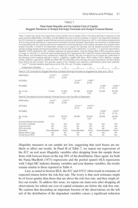
In Panel A of Table 7 we repeat our main tests using ICC estimates thatcorrect for the measurement error due to sluggish analyst forecast revisions us-ing a method proposed by Guay et al. (2011). The idea behind their method isthat analyst forecasts may only reflect information that was impounded in pricesearlier than the current price. Hence, in essence, the method allows analysts extratime to impound the information in recent price movements into their forecasts.As suggested by those authors, we recalculate the ICC using the stock price mea-sured 5 months earlier than in the previous calculation but using the same analystforecasts. For both the Fama-MacBeth (1973) regressions and the pooled (panel)OLS regressions with 3-digit SIC industry dummy variables and year dummyvariables, the results are similar to those in Table 4.
We also do tests that account for potential biases in analyst forecasts notedby Easton and Monahan (2005). The worry is that the calculation of ICC assumesthat the consensus forecast is an unbiased estimate of investors’ expectations, butanalysts make biased forecasts. This should not affect our regressions of the ICCon real asset illiquidity if the forecasts are equally biased for all stocks, but it mayaffect our results if the bias is related to real asset illiquidity. For example, if theforecasts are biased in favor of firms with more illiquid real assets, then for thesefirms the ICC will be biased upward and the effect of real asset illiquidity on theICC would be overstated.
Further investigation shows that biases in analysts’ earnings forecasts do notdrive our results. The correlations of the analyst forecast bias with the real asset
Ortiz-Molina and Phillips 21
TABLE 7
Real Asset Illiquidity and the Implied Cost of Capital:Sluggish Revisions of Analyst Earnings Forecasts and Analyst Forecast Biases
Table 7 reports the results from regressions of the implied cost of capital (ICC) on the three alternative measures of realasset illiquidity (MNoPotBuy, NLPotBuy, and MTotM&A) and a set of control variables. In Panel A, the dependent variable isthe ICC corrected for sluggish analyst forecast revisions using the method of Guay et al. (2011), which allows analysts extratime to impound the information in recent price movements into their forecasts. Specifically, the correction is implementedby recalculating the ICC using the stock price measured 5 months earlier than in the original calculation but using the sameanalyst forecasts. In Panel B, the dependent variable is our original ICC estimate, but the sample excludes firms whosesample-average analyst earnings forecast bias is in the top 30% of the distribution. In columns 1, 3, and 5 we report Fama-MacBeth (1973) regressions with t-statistics adjusted for autocorrelation using the Newey-West (1987) procedure basedon 6 lags. In columns 2, 4, and 6 we report pooled (panel) OLS regressions with 3-digit SIC industry fixed effects and yearfixed effects, and standard errors clustered by 3-digit SIC industry. We also include but do not report the coefficients ofthe following control variables defined in Table 1: LogMCap, LogBM, DRP, BLev, ROE, VolRoe, FA/TA, R&DExp, LogAge,DivPay, SalGrow, LogInvPrice, RetPM, and RetP12M. The estimates of the intercept, the year fixed effects, and the industryfixed effects are also omitted. The absolute values of the t-statistics are reported in parentheses below each estimate.*, **, and *** indicate statistical significance at the 10%, 5%, and 1% levels, respectively.
Independent Variables 1 2 3 4 5 6
Panel A. ICC Corrected for Sluggish Revisions of Analyst Earnings Forecasts as Suggested by Guay et al. (2011)
MNoPotBuy 0.013*** 0.013***(3.71) (3.32)
NLPotBuy 0.014*** 0.009***(9.45) (5.45)
MTotM&A 0.006** 0.004***(2.12) (2.91)
No. of obs. 31,642 31,642 32,338 32,338 32,338 32,338R2 0.57 0.57 0.57
Panel B. Excluding Firms with Analysts’ Forecast Errors in the Top 30% of Distribution
MNoPotBuy 0.015*** 0.015***(4.56) (3.00)
NLPotBuy 0.014*** 0.010***(5.31) (5.83)
MTotM&A 0.008** 0.004**(2.13) (2.13)
No. of obs. 22,072 22,072 22,559 22,559 22,559 22,559R2 0.61 0.61 0.61
Empirical Model (both panels)All control variables Yes Yes Yes Yes Yes YesYear dummies No Yes No Yes No YesSIC3 dummies No Yes No Yes No YesEstimation Fama-MacBeth Panel Fama-MacBeth Panel Fama-MacBeth PanelNewey-West 6 lags Yes No Yes No Yes NoClustering by SIC3 No Yes No Yes No Yes
illiquidity measures in our sample are low, suggesting that such biases are un-likely to affect our results. In Panel B of Table 7, we repeat our regressions ofthe ICC on real asset illiquidity variables after dropping from the sample thosefirms with forecast biases in the top 30% of the distribution. Once again, for boththe Fama-MacBeth (1973) regressions and the pooled (panel) OLS regressionswith 3-digit SIC industry dummy variables and year dummy variables, the resultsremain similar to those reported in Table 4.
Last, as noted in Section III.E, the ICC and FFCC often result in estimates ofexpected returns below the risk-free rate. The worry is that such estimates mightbe of lesser quality than those that are above the risk-free rate, and they might af-fect our results. To address this issue, we repeat our main tests after dropping allobservations for which our cost of capital estimates are below the risk-free rate.We caution that discarding an important fraction of the observations on the lefttail of the distribution of the dependent variables causes a significant reduction

22 Journal of Financial and Quantitative Analysis
in their variation, which diminishes the statistical power of our tests. Neverthe-less, we continue to find a positive and statistically significant relation betweenreal asset illiquidity and both the ICC and the FFCC, albeit of a smaller economicsignificance (see Table A1 and Table A2 of the Online Appendix (www.jfqa.org)).
E. The Distinction Between Inside and Outside Illiquidity
To test our third prediction, in Table 8 we regress the ICC on inside-industryreal asset illiquidity (MInM&A) and outside-industry real asset illiquidity(MOutM&A), which are defined in Section III.B. In columns 1 and 3 we report theresults of Fama-MacBeth (1973) regressions with t-statistics adjusted for autocor-relation using the Newey-West (1987) procedure with 6 lags. In columns 2 and 4we report the results of pooled (panel) OLS regressions with 3-digit SIC industryand year fixed effects, and standard errors clustered at the 3-digit SIC industrylevel.
TABLE 8
Inside versus Outside Real Asset Illiquidity and the Implied Cost of Capital
Table 8 reports the results from regressions of the implied cost of capital (ICC) on two measures of real asset illiquiditydefined in Table 1 (MInM&Q and MOutM&A) and a set of control variables. In columns 1 and 3 we report Fama-MacBeth(1973) regressions with t-statistics adjusted for autocorrelation using the Newey-West (1987) procedure based on 6 lags. Incolumns 2 and 4 we report pooled (panel) OLS regressions with 3-digit SIC industry fixed effects and year fixed effects, andstandard errors clustered by 3-digit SIC industry. We also include but do not report the coefficients of the following controlvariables defined in Table 1: LogMCap, LogBM, DRP, BLev, ROE, VolRoe, FA/TA, R&DExp, LogAge, DivPay, SalGrow,LogInvPrice, RetPM, and RetP12M. The estimates of the intercept, the year fixed effects, and the industry fixed effects arealso omitted. The absolute values of the t-statistics are reported in parentheses below each estimate. *, **, and *** indicatestatistical significance at the 10%, 5%, and 1% levels, respectively.
Independent Variables 1 2 3 4
MInM&A 0.008* 0.005***(2.03) (2.62)
MOutM&A 0.003*** 0.002(3.71) (1.50)
No. of obs. 33,494 33,494 33,494 33,494R2 0.56 0.56
Empirical ModelAll control variables Yes Yes Yes YesYear dummies No Yes No YesSIC3 dummies No Yes No YesEstimation Fama-MacBeth Panel Fama-MacBeth PanelNewey-West 6 lags Yes No Yes NoClustering by SIC3 No Yes No Yes
There is a positive and statistically significant effect of both MInM&A andMOutM&A on the ICC in the cross-sectional tests. Similarly, both MInM&A andMOutM&A increase the ICC in the tests that rely on the time-series variation inasset illiquidity, but the effect of MOutM&A is not statistically significant. Thenew result is that inside illiquidity has a much larger effect on the cost of capitalthan outside illiquidity. The cross-sectional results in columns 1 and 3 imply thata 1-standard-deviation increase in MInM&A increases the ICC by 0.8 percentagepoints, but a similar increase in MOutM&A only increases it by 0.3 percentagepoints. This difference is statistically significant. For the time-series results incolumns 2 and 4, such an increase in MInM&A reduces the cost of capital by0.5 percentage points, but the same increase in MOutM&A reduces it by only 0.2percentage points. This difference is statistically significant.

Ortiz-Molina and Phillips 23
In sum, real asset illiquidity due to weak acquisition activity by industryinsiders has a larger positive impact on the cost of capital than real asset illiquiditydue to weak acquisition activity by industry outsiders. This suggests that inside-industry acquirers can better redeploy the asset than outside acquirers, and thusare willing to pay higher prices. By making real asset markets more illiquid, aweaker presence of inside buyers reduces firms’ operating flexibility by more thana weaker presence of outside buyers, and thus has a larger positive effect on firms’cost of capital.
V. Cross-Sectional Variation in the Effect of Real AssetIlliquidity
To better understand the economic mechanism underlying our findings, wenow explore what drives the variation across firms in the effect of real asset illiq-uidity on the cost of capital. The idea is to identify situations in which real assetilliquidity might cause a stronger covariance of fundamentals with the state of theeconomy and hence have a larger impact on firms’ cost of capital. To this end,we run our main regression of the ICC on MNoPotBuy, NLPotBuy, or MTotM&Awith 3-digit SIC fixed effects and year fixed effects separately for extreme sub-samples and compare the effects. Our predictions 4i to 4iii state that the effectshould be strictly larger in one subsample than in another. However, we use a con-servative approach and compare the effects across groups using two-tailed testsof the null hypothesis that the effects are the same in both subsamples against thebroader alternative hypothesis that they are different.
A. Product Market Competition and Relative Industry Position
In Table 9 we test the prediction that real asset illiquidity should increase thecost of capital more for firms in more competitive industries and for the small-est firms in each industry. In columns 1 and 2, we use the Herfindahl-HirschmanIndex (HHI) of sales concentration to split the sample into firms in high-HHI in-dustries (the least competitive) and in low-HHI industries (the most competitive).Since the Census only reports the HHI for manufacturing industries but our sam-ple contains many nonmanufacturing industries, we calculate a predicted concen-tration index for all industries using the approach in Hoberg and Phillips (2010).13
We then classify industries into those with a predicted HHI in the top tercile ofthe distribution (high HHI) and those with a predicted HHI in the bottom tercileof the distribution (low HHI). The coefficients of MNoPotBuy and MTotM&A arepositive and statistically significant for firms in the low-HHI group, but they aremuch smaller and not significant or marginally significant for firms in the high-HHI group. The coefficient of NLPotBuy does not differ across the two groups.
13In short, we regress concentration indices in manufacturing industries on employment levelsobtained from the Bureau of Labor Statistics as well as on Compustat-based concentration indices andother variables related to concentration. Since our predictors are available for all industries and notjust manufacturing, we then use the estimated coefficients to predict the concentration indices for allindustries in our data.

24 Journal of Financial and Quantitative Analysis
These differences in the coefficients of MNoPotBuy and MTotM&A are highlysuggestive of a larger impact of real asset illiquidity for firms in the low-HHIgroup, but in both cases a two-tailed test is unable to reject the null that the effectof real asset illiquidity is the same in both groups.
TABLE 9
The Role of Industry Concentration and Industry Position
Table 9 reports the results from regressions of the implied cost of capital (ICC) on the three alternative measures of realasset illiquidity defined in Table 1 (MNoPotBuy, NLPotBuy, and MTotM&A) and a set of control variables. All specificationsare pooled (panel) OLS regressions with 3-digit SIC industry fixed effects and year fixed effects, and standard errorsclustered by 3-digit SIC industry. Columns 1 and 2 split the sample into high-concentration industries and low-concentrationindustries according to whether the industry’s predicted sales-based Herfindahl-Hirschman Index (HHI) of concentrationis in the top or bottom tercile of the annual distribution, respectively. Columns 3 and 4 split the sample into industry leaders,defined as firms with at least a 15% market share in their 3-digit SIC industry, and industry followers, defined as those withmarket shares below 15%, respectively. We also include but do not report the coefficients of the following control variablesdefined in Table 1: LogMCap, LogBM, DRP, BLev, ROE, VolRoe, FA/TA, R&DExp, LogAge, DivPay, SalGrow, LogInvPrice,RetPM, and RetP12M. The estimates of the intercept, the year fixed effects, and the industry fixed effects are also omitted.The absolute values of the t-statistics are reported in parentheses below each estimate. *, **, and *** indicate statisticalsignificance at the 10%, 5%, and 1% levels, respectively.
High HHI Low HHI Leaders Followers
1 2 3 4
Panel A. The Measure of Real Asset Illiquidity Is MNoPotBuy
MNoPotBuy 0.007* 0.020** −0.005 0.014***(1.90) (2.24) (0.52) (2.83)
No. of obs. 10,533 10,277 5,397 27,370R2 0.56 0.61 0.58 0.56
Panel B. The Measure of Real Asset Illiquidity Is NLPotBuy
NLPotBuy 0.011*** 0.010*** 0.003** 0.012***(3.04) (4.91) (1.97) (5.93)
No. of obs. 10,757 10,494 5,537 27,957R2 0.57 0.61 0.59 0.57
Panel C. The Measure of Real Asset Illiquidity Is MTotM&A
MTotM&A 0.002 0.007** 0.000 0.006***(1.00) (2.01) (0.37) (2.62)
No. of obs. 10,757 10,494 5,537 27,957R2 0.57 0.61 0.58 0.56
Empirical Model (all panels)All control variables Yes Yes Yes YesEstimation Panel Panel Panel PanelYear dummies Yes Yes Yes YesSIC3 dummies Yes Yes Yes YesClustering by SIC3 Yes Yes Yes Yes
In columns 3 and 4 of Table 9, we split the sample into industry “leaders”and “followers.” As in Campello (2006), we classify as “leaders” those firms withmarket shares of at least 15% in their 3-digit SIC industry and as “followers” thosefirms with market shares below 15%. We find that all of our measures of real assetilliquidity have a large positive and statistically significant impact on the cost ofcapital of followers, but they have little effect on the cost of capital of industryleaders. For leaders, the coefficients of MNoPotBuy and MTotM&A are close to0 and are statistically insignificant, while the coefficient on NLPotBuy is statisti-cally significant and positive but much smaller than for followers. Furthermore,in all cases two-tailed tests reject the null that the effect of real asset illiquidity isthe same for followers and leaders, with p-values of 0.071 for MNoPotBuy, 0.001for NLPotBuy, and 0.018 for MTotM&A, respectively.
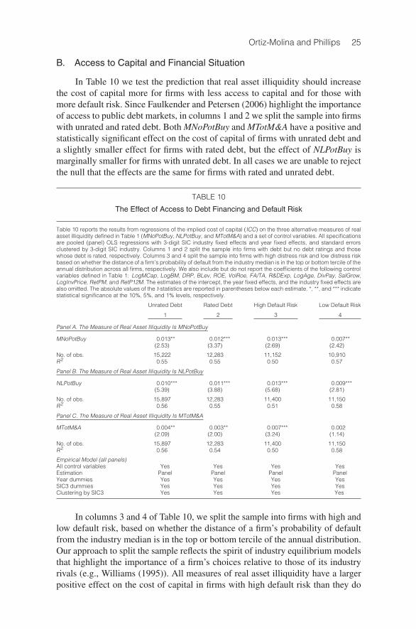
Ortiz-Molina and Phillips 25
B. Access to Capital and Financial Situation
In Table 10 we test the prediction that real asset illiquidity should increasethe cost of capital more for firms with less access to capital and for those withmore default risk. Since Faulkender and Petersen (2006) highlight the importanceof access to public debt markets, in columns 1 and 2 we split the sample into firmswith unrated and rated debt. Both MNoPotBuy and MTotM&A have a positive andstatistically significant effect on the cost of capital of firms with unrated debt anda slightly smaller effect for firms with rated debt, but the effect of NLPotBuy ismarginally smaller for firms with unrated debt. In all cases we are unable to rejectthe null that the effects are the same for firms with rated and unrated debt.
TABLE 10
The Effect of Access to Debt Financing and Default Risk
Table 10 reports the results from regressions of the implied cost of capital (ICC) on the three alternative measures of realasset illiquidity defined in Table 1 (MNoPotBuy, NLPotBuy, and MTotM&A) and a set of control variables. All specificationsare pooled (panel) OLS regressions with 3-digit SIC industry fixed effects and year fixed effects, and standard errorsclustered by 3-digit SIC industry. Columns 1 and 2 split the sample into firms with debt but no debt ratings and thosewhose debt is rated, respectively. Columns 3 and 4 split the sample into firms with high distress risk and low distress riskbased on whether the distance of a firm’s probability of default from the industry median is in the top or bottom tercile of theannual distribution across all firms, respectively. We also include but do not report the coefficients of the following controlvariables defined in Table 1: LogMCap, LogBM, DRP, BLev, ROE, VolRoe, FA/TA, R&DExp, LogAge, DivPay, SalGrow,LogInvPrice, RetPM, and RetP12M. The estimates of the intercept, the year fixed effects, and the industry fixed effects arealso omitted. The absolute values of the t-statistics are reported in parentheses below each estimate. *, **, and *** indicatestatistical significance at the 10%, 5%, and 1% levels, respectively.
Unrated Debt Rated Debt High Default Risk Low Default Risk
1 2 3 4
Panel A. The Measure of Real Asset Illiquidity Is MNoPotBuy
MNoPotBuy 0.013** 0.012*** 0.013*** 0.007**(2.53) (3.37) (2.69) (2.42)
No. of obs. 15,222 12,283 11,152 10,910R2 0.55 0.55 0.50 0.57
Panel B. The Measure of Real Asset Illiquidity Is NLPotBuy
NLPotBuy 0.010*** 0.011*** 0.013*** 0.009***(5.39) (3.88) (5.68) (2.81)
No. of obs. 15,897 12,283 11,400 11,150R2 0.56 0.55 0.51 0.58
Panel C. The Measure of Real Asset Illiquidity Is MTotM&A
MTotM&A 0.004** 0.003** 0.007*** 0.002(2.09) (2.00) (3.24) (1.14)
No. of obs. 15,897 12,283 11,400 11,150R2 0.56 0.54 0.50 0.58
Empirical Model (all panels)All control variables Yes Yes Yes YesEstimation Panel Panel Panel PanelYear dummies Yes Yes Yes YesSIC3 dummies Yes Yes Yes YesClustering by SIC3 Yes Yes Yes Yes
In columns 3 and 4 of Table 10, we split the sample into firms with high andlow default risk, based on whether the distance of a firm’s probability of defaultfrom the industry median is in the top or bottom tercile of the annual distribution.Our approach to split the sample reflects the spirit of industry equilibrium modelsthat highlight the importance of a firm’s choices relative to those of its industryrivals (e.g., Williams (1995)). All measures of real asset illiquidity have a largerpositive effect on the cost of capital in firms with high default risk than they do

26 Journal of Financial and Quantitative Analysis
in firms with low default risk. The effect of MTotM&A is not statistically signif-icant and is close to 0 for firms in the low default risk group. Two-tailed testsreject the null that the effect of real asset illiquidity is the same for firms withhigh and low default risk in the case of NLPotBuy, with a p-value of 0.048, andMTotM&A, with a p-value of 0.014. For MNoPotBuy, the two-tailed p-value is0.153.
C. Business Environment
In Table 11 we test the prediction that real asset illiquidity should increasethe cost of capital more for firms with low valuation and for those in industriesexperiencing downturns. In columns 1 and 2, we split the sample into firms withlow and high market-to-book value of assets (M/B), based on whether the distanceof a firm’s M/B from the industry median is in the bottom or top tercile of theannual distribution. All measures of real asset illiquidity have a larger positiveeffect on the cost of capital for firms with low M/B than they do for firms withhigh M/B. Two-tailed tests reject the null that the effect of real asset illiquidity is
TABLE 11
The Effect of Market Valuations and Demand Shocks
Table 11 reports the results from regressions of the implied cost of capital (ICC) on the three alternative measures of realasset illiquidity defined in Table 1 (MNoPotBuy, NLPotBuy, and MTotM&A) and a set of control variables. All specificationsare pooled (panel) OLS regressions with 3-digit SIC industry fixed effects and year fixed effects, and standard errorsclustered by 3-digit SIC industry (except columns 3 and 4 which have no industry fixed effects). Columns 1 and 2 split thesample into low and high market-to-book value of assets ratios (M/B) based on whether the distance of a firm’s M/B fromthe industry median is in the bottom or top tercile of the annual distribution across all firms, respectively. Columns 3 and 4split the sample into firms in 3-digit SIC industries experiencing an economic downturn and firms in industries that are notexperiencing a downturn, respectively. We also include but do not report the coefficients of the following control variablesdefined in Table 1: LogMCap, LogBM, DRP, BLev, ROE, VolRoe, FA/TA, R&DExp, LogAge, DivPay, SalGrow, LogInvPrice,RetPM, and RetP12M. The estimates of the intercept, the year fixed effects, and the industry fixed effects are also omitted.The absolute values of the t-statistics are reported in parentheses below each estimate. *, **, and *** indicate statisticalsignificance at the 10%, 5%, and 1% levels, respectively.
Low M/B High M/B Industry Downturn Not Industry Downturn
1 2 3 4
Panel A. The Measure of Real Asset Illiquidity Is MNoPotBuy
MNoPotBuy 0.015** 0.013*** 0.012* 0.016***(2.55) (2.74) (1.68) (4.69)
No. of obs. 10,824 11,152 854 31,913R2 0.57 0.54 0.33 0.38
Panel B. The Measure of Real Asset Illiquidity Is NLPotBuy
NLPotBuy 0.013*** 0.010*** 0.032*** 0.017***(5.85) (5.12) (5.20) (6.21)
No. of obs. 11,064 11,400 862 32,632R2 0.58 0.55 0.39 0.39
Panel C. The Measure of Real Asset Illiquidity Is MTotM&A
MTotM&A 0.006*** 0.004** 0.024*** 0.011***(2.76) (2.07) (4.77) (5.04)
No. of obs. 11,064 11,400 862 32,632R2 0.57 0.55 0.40 0.36
Empirical Model (all panels)All control variables Yes Yes Yes YesEstimation Panel Panel Panel PanelYear dummies Yes Yes Yes YesSIC3 dummies Yes Yes No NoClustering by SIC3 Yes Yes Yes Yes

Ortiz-Molina and Phillips 27
the same for firms with high and low M/B in the case of NLPotBuy (the p-valueis 0.002) and MTotM&A (the p-value is 0.044). The two-tailed test cannot rejectthe null that the effect of MNoPotBuy is the same in both groups.
In columns 3 and 4 of Table 11, we split the sample into firms in indus-tries experiencing a downturn and those in industries that are not. As in Oplerand Titman (1994), we identify a 3-digit SIC industry to be in a downturn in agiven year when its median sales growth is negative and its median stock return isbelow −30%. We do not include the 3-digit SIC industry dummy variables inthe regressions because few industries remain in the downturn group for morethan 1 year. All real asset illiquidity measures are positively related to the cost ofcapital and are statistically significant in both samples. The effects of NLPotBuyand MTotM&A are much larger for firms in industries experiencing downturnsthan they are for firms in industries that are not. Two-tailed tests reject the nullthat the effect of real asset illiquidity is the same in both groups with p-valuesof 0.018 for NLPotBuy and of 0.001 for MTotM&A, respectively. The effect ofMNoPotBuy is smaller during downturns, but the difference is small and statisti-cally insignificant.
VI. Additional Tests
We now briefly discuss additional tests whose results are omitted from themain text for brevity but are contained in the paper’s Online Appendix. Unlessotherwise noted, we run both Fama-MacBeth (1973) regressions with t-statisticsadjusted for autocorrelation using the Newey-West (1987) procedure based on6 lags and pooled (panel) OLS regressions with 3-digit SIC industry fixed effectsand year fixed effects, and standard errors clustered by 3-digit SIC industry.
A. Real Asset Illiquidity and the Illiquidity or Systematic Liquidity Risk ofFirms’ Stock
There is a potential concern that our results could be capturing liquidity riskas more illiquid stocks (e.g., Amihud and Mendelson (1986)) and stocks withmore systematic liquidity risk (e.g., Pastor and Stambaugh (2003)) have higherexpected returns. To address this concern, we measure systematic liquidity riskusing PSLiqBeta, defined following Pastor and Stambaugh (2003) as the sensitiv-ity of a stock’s return to their liquidity factor,14 and we measure a stock’s illiquid-ity using the square root version of Amihud’s (2002) measure, AmihudIll.15 The
14For each firm, the loading (βLIQ) on the liquidity factor (LIQ) is estimated with monthly datausing 5-year rolling windows (with at least 36 observations): r − rf = α + βMKT MKT + βSMBSMB +βHMLHML + βLIQLIQ + ε.
15For each firm i and year t,
AmihudIlli,t =1
Ni,t
Ni,t∑j=1
√|Ri, j|/VolDi, j,
where Ni,t is the number of trading days for stock i during year t, Ri, j is the return on day j, andVolDi, j is the trading volume on day j in millions of dollars.

28 Journal of Financial and Quantitative Analysis
effect of real asset illiquidity on the ICC is robust to controlling for PSLiqBetaand AmihudIll or their 3-digit SIC industry value-weighted averages (see TablesA3 and A4).
B. Controlling for Industry Valuation
To explore whether a correlation between the measures of real asset illiq-uidity and industry valuations could drive our results, we repeat our analysesafter controlling for two alternative measures of industry valuations constructedat the 3-digit SIC industry level. The first is the logarithm of the average market-to-book equity ratio in the industry (LogIndMB). The second is the industry’s val-uation relative to historical values (RelIndVal). As in Hoberg and Phillips (2010),we construct this variable as the difference between the industry’s log market-to-book equity ratio and its predicted value from the benchmark specification inPastor and Veronesi (2003). Including these industry valuation measures in ourregression models does not significantly affect the coefficients on MNoPotBuy,NLPotBuy, or MTotM&A (see Table A5).
C. Unlevered Cost of Capital
We study whether an association between real asset illiquidity and finan-cial leverage could drive our results. To this end, we repeat our tests using theunlevered cost of capital, which we estimate by delevering the ICC using theModigliani-Miller formula with taxes, and all the control variables, except that weomit financial leverage.16 The estimated coefficients on MNoPotBuy, NLPotBuy,or MTotM&A are similar in magnitude and statistical significance to those inregression models estimated using the ICC and controlling for leverage(see Table A6).
D. Industry-Level Tests
Our main analyses are based on firm-level regressions of the ICC on mea-sures of real asset illiquidity that are largely measured at the industry level. Analternative estimation approach is to convert the ICC and the control variables into3-digit SIC industry-level (equal-weighted) averages and then estimate the regres-sions at the industry level. Hence, we estimate industry-level regression modelsusing weighted least squares (WLS), wherein the weight on each industry-yearobservation is the number of firms in the industry. We run pooled (panel) OLS
16In addition to market debt-to-equity ratios and the top corporate tax rate, the formula requireseach firm’s cost of debt. We estimate the cost of debt for each firm-year in our sample by mapping afirm’s Standard & Poor’s (S&P) debt rating to the average bond yield in its rating category. Since onlya limited number of firms have credit ratings, we estimate missing credit ratings for other firms. Forthe subset of companies with credit ratings, we estimate an ordered logit model that predicts the S&Pdebt rating. Our predictors are the natural logarithm of a firm’s assets, financial leverage, profitability,interest coverage, the natural logarithm of a firm’s age, and the volatility of excess returns. Next, weuse the estimated coefficients from this model to predict the debt rating for all the companies whoseratings are missing, but have the complete set of predictors. For each year, we match a firm’s debtrating to the average bond yield in its rating category, based on individual yields on new debt issuesobtained from SDC.

Ortiz-Molina and Phillips 29
regressions with year fixed effects and with both 3-digit SIC industry fixed effectsand year fixed effects. In all models we cluster the standard errors by 3-digit SICindustry. We continue to find a positive and statistically significant effect of realasset illiquidity on the cost of capital (see Table A7).
E. Real Asset Illiquidity and Equity Values
Our results suggest that, through its effect on the discount rate, real assetilliquidity has a large impact on firm value. To better gauge the magnitude ofthis impact, we regress the logarithm of the book-to-market equity ratio on thereal asset illiquidity measures and control variables. Using alternative estimationapproaches, we find that all three measures of real asset illiquidity have a neg-ative impact on firm value that is statistically and economically significant aftercontrolling for cash flow effects. These tests, which do not rely on asset pricingmodels as the FFCC does or on assumptions like those used to calculate the ICC,provide further evidence that real asset illiquidity affects firms’ cost of capital andthus their values (see Table A8).
F. Multisegment Firms
Our measures of real asset illiquidity require that we identify each firm’sindustry, which we do using firms’ primary SIC codes. We further refine themeasures to incorporate the segments of multiple-segment firms. We calculatethe real asset illiquidity of a multiple-segment firm as the weighted average realasset illiquidity of each of its 3-digit SIC industry segments, with weights equalto the fraction of a firm’s total assets accounted for by each segment’s assets.For MNoPotBuy and NLPotBuy, which depend on identifying a firm’s industry ri-vals, we consider all rivals, including the secondary segments of multiple-segmentfirms. Tests using segment-weighted measures of real asset illiquidity give resultssimilar to those reported (see Table A9).
VII. Summary and Conclusions
We examine whether a more illiquid market for real (or physical) assetsincreases a firm’s cost of unwinding its capital stock and decreases its ability toraise cash, hence reducing the firm’s flexibility in responding to a changing busi-ness environment. Operating inflexibility can be costly in downturns (a point thathas become very evident during the recent financial crisis). Thus, we hypothesizethat real asset illiquidity reduces a firm’s operating flexibility, and as a result itincreases the cost of capital.
Using measures of real asset illiquidity that capture the industry equilibriumaspect of illiquidity highlighted by Shleifer and Vishny (1992), we find an aggre-gate real asset illiquidity premium in firms’ cost of capital that is strongly counter-cyclical. We also show that firms with more illiquid real assets have a higher costof capital both in cross-sectional and time-series tests. These results are robust tothe worry that measurement error in the cost of capital, which could arise due tobiases or sluggish revisions in the analyst earnings forecasts used to calculate the

30 Journal of Financial and Quantitative Analysis
implied cost of capital, might drive the results. They are also similar if we mea-sure expected returns using the more noisy Fama-French (1993) 3-factor modelcost of capital. For robustness, we also use firm-level measures, which capture theoverall illiquidity of all assets in a firm’s balance sheet, and we continue to find apositive impact of these measures on the cost of capital.
Consistent with Shleifer and Vishny (1992), who model how buyers whooperate inside the industry are willing to pay higher prices for an asset than buy-ers who operate outside the industry, we find that weaker acquisition activity byindustry insiders increases a firm’s cost of capital more than weaker acquisitionactivity by firms of industry outsiders. The effect of real asset illiquidity on thecost of capital also exhibits sensible variation across firms: It is stronger for firmsthat face more competitive risk in product markets, that have less access to exter-nal capital or are closer to default, and for those facing negative demand shocks.These effects are robust to controlling for the systematic liquidity risk of a firm’sstock.
Taken together, our results suggest that real asset illiquidity is a major de-terminant of a firm’s operating flexibility, and that it has an economically signif-icant impact on a firm’s cost of equity capital. Combined with the evidence inBenmelech and Bergman (2009), which shows that real asset illiquidity increasesthe cost of debt, our results also suggest that, by increasing firms’ overall cost ofcapital, real asset illiquidity might affect firms’ investment decisions.
ReferencesAlmeida, H.; M. Campello; and D. Hackbarth. “Liquidity Mergers.” Journal of Financial Economics,
102 (2011), 526–558.Amihud, Y. “Illiquidity and Stock Returns: Cross-Section and Time-Series Effects.” Journal of Finan-
cial Markets, 5 (2002), 31–56.Amihud, Y., and H. Mendelson. “Asset Pricing and the Bid-Ask Spread.” Journal of Financial Eco-
nomics, 17 (1986), 223–249.Benmelech, E., and N. K. Bergman. “Liquidation Values and the Credibility of Financial Contract
Renegotiation: Evidence from U.S. Airlines.” Quarterly Journal of Economics, 123 (2008), 1635–1677.
Benmelech, E., and N. K. Bergman. “Collateral Pricing.” Journal of Financial Economics, 91 (2009),339–360.
Berger, A., and C. Bouwman. “Bank Liquidity Creation.” Review of Financial Studies, 22 (2009),3779–3837.
Berk, J. B. “A Critique of Size-Related Anomalies.” Review of Financial Studies, 8 (1995), 275–286.Bharath, S. T., and T. Shumway. “Forecasting Default with the Merton Distance to Default Model.”
Review of Financial Studies, 21 (2008), 1339–1369.Booth, L. “The Influence of Production Technology on Risk and the Cost of Capital.” Journal of Fi-
nancial and Quantitative Analysis, 26 (1991), 109–127.Campello, M. “Debt Financing: Does It Boost or Hurt Firm Performance in Product Markets?” Jour-
nal of Financial Economics, 82 (2006), 135–172.Campello, M.; J. R. Graham; and C. Harvey. “The Real Effects of Financial Constraints: Evidence
from a Financial Crisis.” Journal of Financial Economics, 97 (2010), 470–487.Carlson, M.; A. Fisher; and R. Giammarino. “Corporate Investment and Asset Price Dynamics: Im-
plications for the Cross-Section of Returns.” Journal of Finance, 59 (2004), 2577–2603.Chan, K. C., and N.-F. Chen. “Structural and Return Characteristics of Small and Large Firms.” Jour-
nal of Finance, 46 (1991), 1467–1484.Chava, S., and A. K. Purnanandam. “Is Default Risk Negatively Related to Stock Returns?” Review of
Financial Studies, 23 (2010), 2523–2559.Chen, H.; M. Kacperczyk; and H. Ortiz-Molina. “Labor Unions, Operating Flexibility, and the Cost
of Equity.” Journal of Financial and Quantitative Analysis, 46 (2011), 25–58.

Ortiz-Molina and Phillips 31
Chen, K. C. W.; Z. Chen; and K. C. J. Wei. “Legal Protection of Investors, Corporate Governance, andthe Cost of Equity Capital.” Journal of Corporate Finance, 15 (2009), 273–289.
Chen, K. C. W.; Z. Chen; and K. C. J. Wei. “Agency Costs of Free Cash Flows and the Effect of Share-holder Rights on the Implied Cost of Capital.” Journal of Financial and Quantitative Analysis, 46(2011), 171–207.
Cooper, I. “Asset Pricing Implications of Nonconvex Adjustment Costs and Irreversibility of Invest-ment.” Journal of Finance, 61 (2006), 139–170.
DeAngelo, H.; L. DeAngelo; and K. H. Wruck. “Asset Liquidity, Debt Covenants, and ManagerialDiscretion in Financial Distress: The Collapse of L. A. Gear.” Journal of Financial Economics, 64(2002), 3–34.
Dhaliwal, D.; S. Heitzman; and O. Z. Li. “Taxes, Leverage, and the Cost of Equity Capital.” Journal ofAccounting Research, 44 (2006), 691–723.
Easton, P. D., and S. J. Monahan. “An Evaluation of Accounting-Based Measures of Expected Re-turns.” Accounting Review, 80 (2005), 501–538.
Elton, E. J. “Expected Return, Realized Return, and Asset Pricing Tests.” Journal of Finance, 54(1999), 1199–1220.
Fama, E. F., and K. R. French. “Common Risk Factors in the Returns on Stocks and Bonds.” Journal ofFinancial Economics, 33 (1993), 3–56.
Fama, E. F., and K. R. French. “Industry Costs of Equity.” Journal of Financial Economics, 43 (1997),153–193.
Fama, E. F., and J. D. MacBeth. “Risk, Return, and Equilibrium: Empirical Tests.” Journal of PoliticalEconomy, 81 (1973), 607–636.
Faulkender, M., and M. A. Petersen. “Does the Source of Capital Affect Capital Structure?” Reviewof Financial Studies, 19 (2006), 45–79.
Francis, J.; R. LaFond; P. M. Olsson; and K. Schipper. “Costs of Equity and Earnings Attributes.”Accounting Review, 79 (2004), 976–1010.
Gavazza, A. “The Role of Trading Frictions in Real Asset Markets.” American Economic Review, 101(2011), 1106–1143.
Gebhardt, W. R.; C. M. C. Lee; and B. Swaminathan. “Toward an Implied Cost of Capital.” Journalof Accounting Research, 39 (2001), 135–176.
Gomes, J.; L. Kogan; and L. Zhang. “Equilibrium Cross-Section of Returns.” Journal of PoliticalEconomy, 111 (2003), 693–732.
Gopalan, R.; O. Kadan; and M. Pevzner. “Asset Liquidity and Stock Liquidity.” Journal of Financialand Quantitative Analysis, 47 (2012), 333–364.
Guay, W.; S. P. Kothari; and S. Shu. “Properties of Implied Cost of Capital Using Analysts’ Forecasts.”Australian Journal of Management, 36 (2011), 125–149.
Hail, L., and C. Leuz. “International Differences in the Cost of Equity Capital: Do Legal Institutionsand Securities Regulation Matter?” Journal of Accounting Research, 44 (2006), 485–531.
Hail, L., and C. Leuz. “Cost of Capital Effects and Changes in Growth Expectations Around U.S.Cross-Listings.” Journal of Financial Economics, 93 (2009), 428–454.
Hoberg, G., and G. Phillips. “Real and Financial Industry Booms and Busts.” Journal of Finance, 65(2010), 45–86.
Hou, K., and D. T. Robinson. “Industry Concentration and Average Stock Returns.” Journal ofFinance, 61 (2006), 1927–1956.
Kogan, L. “An Equilibrium Model of Irreversible Investment.” Journal of Financial Economics, 62(2001), 201–245.
Kogan, L. “Asset Prices and Real Investment.” Journal of Financial Economics, 73 (2004), 411–431.Lakonishok, J.; A. Shleifer; and R. W. Vishny. “Contrarian Investment, Extrapolation, and Risk.”
Journal of Finance, 49 (1994), 1541–1578.Lang, L.; A. Poulsen; and R. M. Stulz. “Asset Sales, Firm Performance, and the Agency Costs of
Managerial Discretion.” Journal of Financial Economics, 37 (1995), 3–37.Lee, C. M. C.; D. Ng; and B. Swaminathan. “Testing International Asset Pricing Models Using
Implied Cost of Capital.” Journal of Financial and Quantitative Analysis, 44 (2009), 307–305.
Lev, B. “On the Association Between Operating Leverage and Risk.” Journal of Financial and Quan-titative Analysis, 9 (1974), 627–641.
Lundblad, C. “The Risk Return Tradeoff in the Long Run: 1836–2003.” Journal of Financial Eco-nomics, 85 (2007), 123–150.
Maksimovic, V., and G. Phillips. “Asset Efficiency and the Reallocation Decisions of Bankrupt Firms.”Journal of Finance, 53 (1998), 1495–1532.
Maksimovic, V., and G. Phillips. “The Market for Corporate Assets: Who Engages in Mergers andAsset Sales and Are There Efficiency Gains?” Journal of Finance, 61 (2001), 2019–2065.

32 Journal of Financial and Quantitative Analysis
Mandelker, G. N., and S. G. Rhee. “The Impact of the Degrees of Operating and Financial Leverageon Systematic Risk of Common Stock.” Journal of Financial and Quantitative Analysis, 19 (1984),45–57.
Newey, W. K., and K. D. West. “A Simple, Positive Semi-Definite, Heteroskedasticity and Autocorre-lation Consistent Covariance Matrix.” Econometrica, 55 (1987), 703–708.
Opler, T. C., and S. Titman. “Financial Distress and Corporate Performance.” Journal of Finance, 49(1994), 1015–1040.
Pastor, L.; M. Sinha; and B. Swaminathan. “Estimating the Intertemporal Risk-Return Tradeoff Usingthe Implied Cost of Capital.” Journal of Finance, 63 (2008), 2859–2897.
Pastor, L., and R. F. Stambaugh. “Costs of Equity Capital and Model Mispricing.” Journal of Finance,54 (1999), 67–121.
Pastor, L., and R. F. Stambaugh. “Stock Liquidity Risk and Expected Stock Returns.” Journal ofPolitical Economy, 111 (2003), 642–685.
Pastor, L., and P. Veronesi. “Stock Valuation and Learning About Profitability.” Journal of Finance,58 (2003), 1749–1789.
Pulvino, T. C. “Do Asset Fire Sales Exist? An Empirical Investigation of Commercial Aircraft Trans-actions.” Journal of Finance, 53 (1998), 939–975.
Ramey, V. A., and M. D. Shapiro. “Displaced Capital: A Study of Aerospace Plant Closings.” Journalof Political Economy, 109 (2001), 958–992.
Rubinstein, M. E. “A Mean-Variance Synthesis of Corporate Financial Theory.” Journal of Finance,28 (1973), 167–181.
Schlingemann, F. P.; R. M. Stulz; and R. A. Walkling. “Divestitures and the Liquidity of the Marketfor Corporate Assets.” Journal of Financial Economics, 64 (2002), 117–144.
Sharma, A. “Qwest’s Long-Distance Arm Draws Bids Below Targets.” The Wall Street Journal (June 5,2009).
Shleifer, A., and R. W. Vishny. “Liquidation Values and Debt Capacity: A Market Equilibrium Ap-proach.” Journal of Finance, 47 (1992), 1343–1366.
Sibilkov, V. “Asset Liquidity and Capital Structure.” Journal of Financial and Quantitative Analysis,44 (2009), 1173–1196.
Williams, J. T. “Financial and Industry Structure with Agency.” Review of Financial Studies, 8 (1995),431–474.
Zhang, L. “The Value Premium.” Journal of Finance, 60 (2005), 67–103.