ABSTRACT DEEP NEURAL NETWORKS AND REGRESSION …

ABSTRACT

Title of dissertation: DEEP NEURAL NETWORKS ANDREGRESSION MODELS FOR OBJECTDETECTION AND POSE ESTIMATION

Kota Hara, Doctor of Philosophy, 2016

Dissertation directed by: Professor Rama ChellappaDepartment of Electrical and Computer Engineering

Estimating the pose, orientation and the location of objects has been a central prob-

lem addressed by the computer vision community for decades. In this dissertation, we

propose new approaches for these important problems using deep neural networks as

well as tree-based regression models.

For the first topic, we look at the human body pose estimation problem and pro-

pose a novel regression-based approach. The goal of human body pose estimation is to

predict the locations of body joints, given an image of a person. Due to significant vari-

ations introduced by pose, clothing and body styles, it is extremely difficult to address

this task by a standard application of the regression method. Thus, we address this task

by dividing the whole body pose estimation problem into a set of local pose estimation

problems by introducing a dependency graph which describes the dependency among dif-

ferent body joints. For each local pose estimation problem, we train a boosted regression

tree model and estimate the pose by progressively applying the regression along the paths

in a dependency graph starting from the root node.

Our next work is on improving the traditional regression tree method and demon-

strate its effectiveness for pose/orientation estimation tasks. The main issues of the tra-

ditional regression training are, 1) the node splitting is limited to binary splitting, 2) the

form of the splitting function is limited to thresholding on a single dimension of the in-

put vector and 3) the best splitting function is found by exhaustive search. We propose a

novel node splitting algorithm for regression tree training which does not have the issues

mentioned above. The algorithm proceeds by first applying k-means clustering in the

output space, conducting multi-class classification by support vector machine (SVM) and

determining the constant estimate at each leaf node. We apply the regression forest that

includes our regression tree models to head pose estimation, car orientation estimation

and pedestrian orientation estimation tasks and demonstrate its superiority over various

standard regression methods.

Next, we turn our attention to the role of pose information for the object detec-

tion task. In particular, we focus on the detection of fashion items a person is wearing

or carrying. It is clear that the locations of these items are strongly correlated with the

pose of the person. To address this task, we first generate a set of candidate bounding

boxes by using an object proposal algorithm. For each candidate bounding box, image

features are extracted by a deep convolutional neural network pre-trained on a large image

dataset and the detection scores are generated by SVMs. We introduce a pose-dependent

prior on the geometry of the bounding boxes and combine it with the SVM scores. We

demonstrate that the proposed algorithm achieves significant improvement in the detec-

tion performance.

Lastly, we address the object detection task by exploring a way to incorporate an

attention mechanism into the detection algorithm. Humans have the capability of allocat-

ing multiple fixation points, each of which attends to different locations and scales of the

scene. However, such a mechanism is missing in the current state-of-the-art object de-

tection methods. Inspired by the human vision system, we propose a novel deep network

architecture that imitates this attention mechanism. For detecting objects in an image,

the network adaptively places a sequence of glimpses at different locations in the image.

Evidences of the presence of an object and its location are extracted from these glimpses,

which are then fused for estimating the object class and bounding box coordinates. Due

to the lack of ground truth annotations for the visual attention mechanism, we train our

network using a reinforcement learning algorithm. Experiment results on standard ob-

ject detection benchmarks show that the proposed network consistently outperforms the

baseline networks that do not employ the attention mechanism.

DEEP NEURAL NETWORKS AND REGRESSION MODELSFOR OBJECT DETECTION AND POSE ESTIMATION

by

Kota Hara

Dissertation submitted to the Faculty of the Graduate School of theUniversity of Maryland, College Park in partial fulfillment

of the requirements for the degree ofDoctor of Philosophy

2016

Advisory Committee:Professor Rama Chellappa, Chair/AdvisorProfessor Larry DavisProfessor Min WuProfessor Uzi VishkinProfessor Amitabh Varshney

c© Copyright byKota Hara

2016

Dedication

To my parents.

ii

Acknowledgments

The work presented in this dissertation would not have been possible without the

support of several individuals to whom I owe my gratitude.

First, I would like to thank my advisor, Professor Rama Chellappa for giving me

an opportunity to work on challenging and exciting projects over the past five years.

Throughout my studies, he has been always supporting, encouraging and directing me,

especially when I had hard times. It has been such a privilege to work with and learn

from such an extraordinary individual and I am truly honored to be among those who call

him their mentor.

I would like to thank Dr. Robinson Piramuthu and Dr. Vignesh Jagadeesh who

helped and guided me throughout my unforgettable internship at eBay Inc in the summer

of 2014, Dr. Ming-Yu Liu, Dr. Oncel Tuzel and Dr. Amir-massoud Farahmand who pro-

vided enormous supports during my exciting internship at Mitsubishi Electric Research

Labs in 2015-2016. These two internships helped me to expand my knowledge and skills,

which will be enormously useful for my future career. I would also like to thank Professor

Larry Davis, Professor Min Wu, Professor Uzi Vishkin and Professor Amitabh Varshney

for agreeing to serve on my dissertation committee and for sparing their invaluable time

reviewing the work presented here.

During my studies, I was fortunate enough to have many brilliant colleagues at the

University of Maryland who have enriched my graduate life in many ways. A special

mention goes to Dr. Vishal Patel who have been always willing to help me and have been

a great role model for me, and Raviteja Vemulapalli who has been the best labmate one

iii

could have and I would like to thank his various comments and feedback through many

discussions we had for the last five years.

I owe my deepest thanks to my parents who have always stood by me and motivated

me through my career. My special gratitude goes to my wife Eriko for her constant

encouragement and support, without which the pages of this dissertation would be blank.

Finally, this dissertation was supported by a MURI Grant N00014-10-1-0934 from

the Office of Naval Research.

iv

Table of Contents

List of Tables viii

List of Figures x

1 Introduction 11.1 Human Body Pose Estimation by Regression on a Dependency Graph . . 11.2 Growing Regression Tree Forests by Classification for Continuous Object

Pose Estimation . . . . . . . . . . . . . . . . . . . . . . . . . . . . . . . 21.3 Fashion Apparel Detection: the Role of Deep Convolutional Neural Net-

work and Pose-dependent Priors . . . . . . . . . . . . . . . . . . . . . . 31.4 Attentional Network for Visual Object Detection . . . . . . . . . . . . . 41.5 Dissertation Organization . . . . . . . . . . . . . . . . . . . . . . . . . . 4

2 Human Body Pose Estimation by Regression on a Dependency Graph 62.1 Related work . . . . . . . . . . . . . . . . . . . . . . . . . . . . . . . . 82.2 Method - Regression on a Dependency Graph . . . . . . . . . . . . . . . 102.3 Multidimensional Output Regression on Weighted Training Samples . . . 12

2.3.1 Multidimensional Output Regression Tree on Weighted TrainingSamples . . . . . . . . . . . . . . . . . . . . . . . . . . . . . . . 13

2.3.2 Multidimensional Output Boosted Regression Trees on WeightedTraining Samples . . . . . . . . . . . . . . . . . . . . . . . . . . 14

2.3.3 Importance Weighted Boosted Regression Trees . . . . . . . . . 162.4 Experiments . . . . . . . . . . . . . . . . . . . . . . . . . . . . . . . . . 17

2.4.1 Datasets . . . . . . . . . . . . . . . . . . . . . . . . . . . . . . . 172.4.2 Implementation Details . . . . . . . . . . . . . . . . . . . . . . . 192.4.3 Results . . . . . . . . . . . . . . . . . . . . . . . . . . . . . . . 20

2.5 Conclusion . . . . . . . . . . . . . . . . . . . . . . . . . . . . . . . . . 242.6 Acknowledgments . . . . . . . . . . . . . . . . . . . . . . . . . . . . . 25

3 Growing Regression Tree Forests by Classification for Continuous Object PoseEstimation 29

3.0.1 K-clusters Regression Forest . . . . . . . . . . . . . . . . . . . . 31

v

3.0.2 Voting-based ensemble . . . . . . . . . . . . . . . . . . . . . . . 323.0.3 Bootstrap sampling for data imbalanceness problem . . . . . . . 323.0.4 Object pose estimation tasks . . . . . . . . . . . . . . . . . . . . 333.0.5 Summary of the results . . . . . . . . . . . . . . . . . . . . . . . 353.0.6 Organization . . . . . . . . . . . . . . . . . . . . . . . . . . . . 36

3.1 Related work . . . . . . . . . . . . . . . . . . . . . . . . . . . . . . . . 373.1.1 Regression . . . . . . . . . . . . . . . . . . . . . . . . . . . . . 373.1.2 Decision trees with multiway splitting . . . . . . . . . . . . . . . 383.1.3 Sample weighting for data imbalanceness problem . . . . . . . . 393.1.4 Mean shift for a circular space . . . . . . . . . . . . . . . . . . . 403.1.5 Applications . . . . . . . . . . . . . . . . . . . . . . . . . . . . 40

3.1.5.1 Head pose estimation . . . . . . . . . . . . . . . . . . 403.1.5.2 Car direction estimation . . . . . . . . . . . . . . . . . 413.1.5.3 Pedestrian orientation estimation . . . . . . . . . . . . 42

3.2 Methods . . . . . . . . . . . . . . . . . . . . . . . . . . . . . . . . . . . 433.2.1 Abstracted Regression Tree Model . . . . . . . . . . . . . . . . . 443.2.2 Standard Binary Node Splitting . . . . . . . . . . . . . . . . . . 463.2.3 Proposed Node Splitting . . . . . . . . . . . . . . . . . . . . . . 473.2.4 Adaptive determination of K . . . . . . . . . . . . . . . . . . . . 483.2.5 Modification for a Circular Target Space . . . . . . . . . . . . . . 513.2.6 Random Regression Forest . . . . . . . . . . . . . . . . . . . . . 543.2.7 Further extensions . . . . . . . . . . . . . . . . . . . . . . . . . 55

3.2.7.1 Sample weighting technique for imbalanced training data 563.2.7.2 Voting-based ensemble using the mean shift algorithm . 573.2.7.3 Mean shift algorithm for a circular space . . . . . . . . 58

3.3 Experiments . . . . . . . . . . . . . . . . . . . . . . . . . . . . . . . . . 613.3.1 Head Pose Estimation . . . . . . . . . . . . . . . . . . . . . . . 61

3.3.1.1 Dataset and image features . . . . . . . . . . . . . . . 613.3.1.2 Results . . . . . . . . . . . . . . . . . . . . . . . . . . 62

3.3.2 Car Direction Estimation . . . . . . . . . . . . . . . . . . . . . . 663.3.2.1 Dataset and image features . . . . . . . . . . . . . . . 663.3.2.2 Results . . . . . . . . . . . . . . . . . . . . . . . . . . 67

3.3.3 Continuous Pedestrian Orientation Estimation . . . . . . . . . . . 683.3.3.1 Dataset . . . . . . . . . . . . . . . . . . . . . . . . . . 683.3.3.2 Annotation of continuous orientations . . . . . . . . . 693.3.3.3 Image features . . . . . . . . . . . . . . . . . . . . . . 713.3.3.4 Performance measure . . . . . . . . . . . . . . . . . . 723.3.3.5 Evaluated methods . . . . . . . . . . . . . . . . . . . . 723.3.3.6 Additional baseline methods . . . . . . . . . . . . . . 733.3.3.7 Results . . . . . . . . . . . . . . . . . . . . . . . . . . 73

3.4 Conclusions . . . . . . . . . . . . . . . . . . . . . . . . . . . . . . . . . 753.5 Acknowledgments . . . . . . . . . . . . . . . . . . . . . . . . . . . . . 75

vi

4 Fashion Apparel Detection: the Role of Deep Convolutional Neural Network andPose-dependent Priors 824.1 Related Work . . . . . . . . . . . . . . . . . . . . . . . . . . . . . . . . 844.2 Proposed Method . . . . . . . . . . . . . . . . . . . . . . . . . . . . . . 87

4.2.1 Object Proposal . . . . . . . . . . . . . . . . . . . . . . . . . . . 884.2.2 Image Features by CNN . . . . . . . . . . . . . . . . . . . . . . 894.2.3 SVM training . . . . . . . . . . . . . . . . . . . . . . . . . . . . 904.2.4 Probabilistic formulation . . . . . . . . . . . . . . . . . . . . . . 904.2.5 Appearance-based Posterior . . . . . . . . . . . . . . . . . . . . 914.2.6 Geometric Priors . . . . . . . . . . . . . . . . . . . . . . . . . . 92

4.3 Experiments . . . . . . . . . . . . . . . . . . . . . . . . . . . . . . . . . 954.3.1 Dataset . . . . . . . . . . . . . . . . . . . . . . . . . . . . . . . 954.3.2 Detector Training . . . . . . . . . . . . . . . . . . . . . . . . . . 974.3.3 Baseline Methods . . . . . . . . . . . . . . . . . . . . . . . . . . 984.3.4 Results . . . . . . . . . . . . . . . . . . . . . . . . . . . . . . . 98

4.4 Conclusion . . . . . . . . . . . . . . . . . . . . . . . . . . . . . . . . . 1014.5 Acknowledgments . . . . . . . . . . . . . . . . . . . . . . . . . . . . . 101

5 Attentional Network for Visual Object Detection 1075.1 Related Work . . . . . . . . . . . . . . . . . . . . . . . . . . . . . . . . 1085.2 Attention-based Object Detection Network . . . . . . . . . . . . . . . . . 111

5.2.1 Network Architecture . . . . . . . . . . . . . . . . . . . . . . . . 1115.2.2 Reinforcement learning . . . . . . . . . . . . . . . . . . . . . . . 1145.2.3 Network Training . . . . . . . . . . . . . . . . . . . . . . . . . . 116

5.2.3.1 Return Normalization . . . . . . . . . . . . . . . . . . 1185.2.4 Implementation Details . . . . . . . . . . . . . . . . . . . . . . . 119

5.2.4.1 Glimpse features . . . . . . . . . . . . . . . . . . . . . 1195.2.4.2 Training sample construction . . . . . . . . . . . . . . 1205.2.4.3 SGD hyper parameters . . . . . . . . . . . . . . . . . 1205.2.4.4 Underlying Convolutional Network . . . . . . . . . . . 1215.2.4.5 Other default settings . . . . . . . . . . . . . . . . . . 121

5.3 Main Results . . . . . . . . . . . . . . . . . . . . . . . . . . . . . . . . 1225.4 Design Evaluation . . . . . . . . . . . . . . . . . . . . . . . . . . . . . . 1245.5 Conclusion . . . . . . . . . . . . . . . . . . . . . . . . . . . . . . . . . 1295.6 Acknowledgments . . . . . . . . . . . . . . . . . . . . . . . . . . . . . 129

6 Summary and Directions for Future Work 1306.1 Directions for Future Research . . . . . . . . . . . . . . . . . . . . . . . 131

6.1.1 Human Body Pose Estimation by Regression on a DependencyGraph . . . . . . . . . . . . . . . . . . . . . . . . . . . . . . . . 131

6.1.2 Growing Regression Tree Forests by Classification for Continu-ous Object Pose Estimation . . . . . . . . . . . . . . . . . . . . 132

6.1.3 Fashion Apparel Detection: the Role of Deep Convolutional Neu-ral Network and Pose-dependent Priors . . . . . . . . . . . . . . 132

6.1.4 Attentional Network for Visual Object Detection . . . . . . . . . 133

vii

List of Tables

2.1 PCP0.5 on Buffy with the original PCP tool and detection windows . . . 222.2 PCP0.5 on Buffy with the updated PCP tool and detection windows . . . 232.3 PCP0.5 on PASCAL with the original PCP tool and detection windows . 242.4 PCP0.5 on PASCAL with the updated PCP tool and detection windows . 252.5 Computation time per image. Left: our methods, Right: existing methods 262.6 PCP0.5 of importance weighted boosted regression trees on Buffy . . . . 282.7 PCP0.5 of importance weighted boosted regression trees on PASCAL . . 28

3.1 MAE in degree of different regression methods on the Pointing’04 dataset(even train/test split). Time to process one image including HOG compu-tation is also shown. . . . . . . . . . . . . . . . . . . . . . . . . . . . . . 63

3.2 Head pose estimation results on the Pointing’04 dataset (5-fold cross-validation) . . . . . . . . . . . . . . . . . . . . . . . . . . . . . . . . . . 64

3.3 Car direction estimation results on the EPFL Multi-view Car Dataset . . . 763.4 Continuous pedestrian orientation estimation: Accuracy-22.5◦, Accuracy-

45◦ and Mean Absolute Error in degree are shown for AKRF-VW and allbaseline methods. . . . . . . . . . . . . . . . . . . . . . . . . . . . . . 78

3.5 Results of previously proposed approaches. Note that the performance ismeasured differently for the previous approaches as the original discreteannotations are used. See text for the details. All the results are on theTUD Multiview Pedestrians Dataset [Andriluka et al., 2010] . . . . . . . 80

4.1 The definition of new classes, their average size and the average num-ber of occurrence per image are shown. The top 2 key body joints foreach item as selected by the proposed algorithm are also shown. See Sec-tion 4.3.1 for details. . . . . . . . . . . . . . . . . . . . . . . . . . . . . 102

4.2 Average Precision of each method. “Full” achieves better mAP and APsfor all the items than “w/o geometric priors” and “w/o appearance”. . . . 103

4.3 The number of training patches generated for each class with SelectiveSearch Uijlings et al. [2013]. . . . . . . . . . . . . . . . . . . . . . . . . 103

viii

4.4 Precision, recall and the average number of generated bounding boxes perimage. Note that it is important to have high recall and not necessarilyprecision so that we will not miss too many true objects. Precision iscontrolled later by the classification stage. . . . . . . . . . . . . . . . . . 104

5.1 The experimental settings . . . . . . . . . . . . . . . . . . . . . . . . . . 1235.2 Average Precision of methods using CaffeNet under the VOC 2007 setting 1265.3 Average Precision of methods using VGG16 under the VOC 2007 setting 1265.4 Average Precision of methods using VGG16 under the VOC 2012 setting 1265.5 Average Precision of methods using VGG16 under the VOC 2007+2012

setting . . . . . . . . . . . . . . . . . . . . . . . . . . . . . . . . . . . . 1265.6 Average Precision of methods using VGG16 under VOC 2007++2012

setting . . . . . . . . . . . . . . . . . . . . . . . . . . . . . . . . . . . . 1265.7 The effect of the number of episodes generated from one sample in a

mini-batch . . . . . . . . . . . . . . . . . . . . . . . . . . . . . . . . . . 1275.8 The effect of the network architecture . . . . . . . . . . . . . . . . . . . 1275.9 The effect of the reinforcement baseline methods . . . . . . . . . . . . . 1275.10 The effect of the choice between continuous return and discrete return . . 1285.11 The effect of excluding background samples . . . . . . . . . . . . . . . . 1285.12 The effect of the glimpse representation . . . . . . . . . . . . . . . . . . 128

ix

List of Figures

2.1 Left: Dependency graph, Right: Semantics of the nodes. The red boxis a detection window and the yellow star is the center of the detectionwindow. . . . . . . . . . . . . . . . . . . . . . . . . . . . . . . . . . . . 12

2.2 PCP curves with the second setting (best viewed in color) . . . . . . . . 262.3 Representative results of RoDG-Boost on Buffy Stickmen dataset. . . . . 272.4 Representative results of RoDG-Boost on PASCAL Stickmen dataset.

The last two columns show failure cases. . . . . . . . . . . . . . . . . . 27

3.1 User interface for the continuous orientation annotation. Each annotatoris requested to specify the body orientation of pedestrians by moving aline segment in a circle. . . . . . . . . . . . . . . . . . . . . . . . . . . 36

3.2 An illustration of the proposed splitting method (K = 3). A set of clus-ters of the training data is found in the target space by k-means (left). Theinput partitions preserving the found clusters as much as possible are de-termined by an SVM (middle). If no more splitting is needed, a mean iscomputed as a constant estimate for each set of colored samples. The yel-low stars represent the means (right). Note that the color of some pointschange due to misclassification. If additional splitting is needed, clus-terling is applied to each set of colored samples separately in the targetspace. . . . . . . . . . . . . . . . . . . . . . . . . . . . . . . . . . . . . 49

3.3 Pointing’04: The effect of K of KRF on the average MAE. “CV” indi-cates the value of KRF selected by cross-validation. . . . . . . . . . . . 65

3.4 Some estimation results of the second sequence of person 13. The topnumbers are the ground truth yaw and pitch and the bottom numbers arethe estimated yaw and pitch. . . . . . . . . . . . . . . . . . . . . . . . . 66

3.5 EPFL Multi-view Car Dataset: a histogram obtained from the directionson the training data. The car directions are not uniformly distributed. . . 67

3.6 MAE of AKRF computed on each sequence in the testing set of the EPFLMultiview Car Dataset . . . . . . . . . . . . . . . . . . . . . . . . . . . 69

3.7 Representative results from the worst three sequences in the testing set.The numbers under each image are the ground truth direction (left) andthe estimated direction (right). Most of the failure cases are due to theflipping error. . . . . . . . . . . . . . . . . . . . . . . . . . . . . . . . . 70

x

3.8 EPFL Multi-view Car: The effect of K of KRF on MAE. “CV” indicatesthe value of KRF selected by cross-validation. . . . . . . . . . . . . . . 71

3.9 Training samples for representative orientation angles are shown. Foreach angle in {0◦, 10◦, . . . , 350◦}, a training sample with the closest groundtruth is selected. The left-top image corresponds to 0◦ and the right-bottom one corresponds to 350◦. The continuous annotations capturesmooth transition of the body orientations even though the annotationsare done solely from the 2D images. . . . . . . . . . . . . . . . . . . . . 77

3.10 TUD Multiview Pedestrians Dataset: a histogram obtained from the ori-entations on the training data. The orientations are higly imbalanced. . . 78

3.11 Change of the accuracy by varying threshold on the pedestrian orientationestimation task . . . . . . . . . . . . . . . . . . . . . . . . . . . . . . . 79

3.12 Example results from AKRF-VW. Red lines indicate ground truth ori-entations. Blue lines indicate predicted orientations. The first two rowsshow successful cases while the last row shows failure cases. Note thatmany of the failure cases are due to the flipping errors. . . . . . . . . . . 81

4.1 Bounding boxes of three different instances of “skirt” class. The aspectratios vary significantly even though they are from the same object class. . 85

4.2 Overview of the proposed algorithm for testing stage. Object proposalsare generated and features are extracted using Deep CNN from each ob-ject proposal. An array of 1-vs-rest SVMs are used to generate appearance-based posteriors for each class. Geometric priors are tailored based onpose estimation and used to modify the class probability. Non-maximumsuppression is used to arbitrate overlapping detections with appreciableclass probability. . . . . . . . . . . . . . . . . . . . . . . . . . . . . . . 87

4.3 Distributions of relative location of item with respect to location of keyjoint. Key joint location is depicted as a red cross. (a) distribution ofrelative location of bag with respect to neck is multi-modal. (b) locationsof left shoe and left ankle are strongly correlated and the distribution oftheir relative location has a single mode. See Section 4.2.6 for details. . . 93

4.4 Precision-Recall curves for each fashion category. Our full method out-performs the baseline method (shown by cross) with a large margin (some-times up to 10 times in precision for the same recall), except for “Pants”.Note that we do not have results from the baseline methods for “Leftshoe” and “Right shoe” as they are newly defined in this work. . . . . . . 100

4.5 Example detection results obtained by the proposed method. Note thatwe manually overlaid the text labels to improve legibility. . . . . . . . . . 105

4.6 Examples of failed detection results obtained by the proposed method.Note that we overlaid text labels manually to improve legibility. Incorrectlabels are shown in red. . . . . . . . . . . . . . . . . . . . . . . . . . . . 106

5.1 Humans have the capability of using multiple fixation points to accumu-late evidences for detecting objects in a scene. . . . . . . . . . . . . . . . 111

xi

5.2 Illustration of the AOD network: the network consists a stacked recurrent mod-ule designed for object class recognition, bounding box regression and glimpsegeneration. The classification and bounding box regression are done only at thefinal time step while the glimpse generation is done at all time steps except thelast time step. Given an input image, first, a set of feature maps are computedby the Deep Convolutional Neural Network. Given a proposal bounding box att = 1, a fixed dimensional feature vector is extracted from the proposal bound-ing box on the last feature map by the ROI pooling layer [Girshick, 2015]. Afew fully connected layers (fc6 and fc7 in the figure), each followed by a ReLUand dropout layers, are then applied to the extracted feature vector. From the re-sultant features, a next glimpse bounding box is determined by applying a fullyconnected layer. At t = 2, a feature vector is extracted from the glimpse bound-ing box region using the ROI pooling layer. The process is repeated until the lasttime step t = T . At the last time step, an element-wise max operation is appliedto the final feature vectors at all time steps and then softmax classification andbounding box regression are conducted. . . . . . . . . . . . . . . . . . . . . 112

5.3 Representative detection results. White, blue, yellow and red boundingboxes represent object proposals, the first glimpses, the second glimpsesand the final localization results, respectively. . . . . . . . . . . . . . . . 125

xii

Chapter 1: Introduction

In this dissertation, we address a variety of computer vision tasks involving object

poses, orientations and locations. First, we propose an efficient regression-based algo-

rithm for the task of human body pose estimation. The algorithm consists of a series of

regressions, each of which is responsible only for the local pose estimation task. Sec-

ondly, we point out several issues in the standard regression tree training algorithm and

propose a novel node splitting method for regression tree training based on k-means clus-

tering and SVM. We then apply this method to several object pose estimation tasks. Next,

we study the role of human pose for detecting the fashion items. We introduce a pose-

dependent prior on the geometry of the object bounding boxes and integrate it with a

state-of-the-art object detector trained on our dataset. Finally, in order to incorporate an

attention mechanism into an object detection method, we propose a deep recurrent neural

network model trained by a reinforcement learning technique. We briefly describe these

topics below.

1.1 Human Body Pose Estimation by Regression on a Dependency Graph

We present a hierarchical method for human pose estimation from a single still

image. In our approach, a dependency graph representing relationships between refer-

1

ence points such as body joints is constructed and the positions of these reference points

are sequentially estimated by the successive application of multidimensional output re-

gressions along the dependency paths, starting from the root node. Each regressor takes

image features computed from an image patch centered on the current node’s position

estimated by the previous regressor and is specialized for estimating its child nodes’ po-

sitions. The use of the dependency graph allows us to decompose a complex pose esti-

mation problem into a set of local pose estimation problems that are less complex. We

design a dependency graph for two commonly used human pose estimation datasets, the

Buffy Stickmen dataset and the ETHZ PASCAL Stickmen dataset, and demonstrate that

our method achieves accuracy comparable to state-of-the-art results on both datasets with

significantly lower computation time. Furthermore, we propose an importance weighted

boosted regression trees method for transductive learning settings and demonstrate the

resulting improved performance for pose estimation tasks.

1.2 Growing Regression Tree Forests by Classification for Continuous

Object Pose Estimation

In this work, we propose a novel node splitting method for regression trees and

incorporate it into the random regression forest framework. Unlike traditional binary

splitting, where the splitting rule is selected from a predefined set of binary splitting

rules via trial-and-error, the proposed node splitting method first finds clusters of the

training data which at least locally minimize the empirical loss without considering the

input space. Then splitting rules which preserve the found clusters as much as possible,

2

are determined by casting the problem as a classification problem. Consequently, our

new node splitting method enjoys more freedom in choosing the splitting rules, resulting

in more efficient tree structures. In addition to the algorithm for the ordinary Euclidean

target space, we present a variant which can naturally deal with a circular target space

by the proper use of circular statistics. In order to deal with challenging, ambiguous

image-based pose estimation problems, we also present a voting-based ensemble method

using the mean shift algorithm. Furthermore, to address the data imbalance problems

present in some of the datasets, we propose a bootstrap sampling method using a sample

weighting technique. We apply the proposed random regression forest algorithm to head

pose estimation, car direction estimation and pedestrian orientation estimation tasks, and

demonstrate its competitive performance.

1.3 Fashion Apparel Detection: the Role of Deep Convolutional Neural

Network and Pose-dependent Priors

In this work, we propose and address a new computer vision task, which we call

fashion item detection, where the aim is to detect various fashion items a person in the

image is wearing or carrying. The types of fashion items we consider in this work include

hat, glasses, bag, pants, shoes and so on. The detection of fashion items can be an im-

portant first step in various e-commerce applications in fashion industry. Our method is

based on a state-of-the-art object detection method which combines object proposal meth-

ods with a Deep Convolutional Neural Network. Since the locations of fashion items are

in strong correlation with the locations of body joints positions, we propose a hybrid

3

discriminative-generative model to incorporate contextual information from body poses

in order to improve the detection performance. Through experiments, we demonstrate

that our algorithm outperforms baseline methods by a large margin.

1.4 Attentional Network for Visual Object Detection

We propose augmenting deep neural networks with an attention mechanism for the

visual object detection task. It is believed that humans have the capability of analyzing

scene contents from multiple fixation points. However, such a mechanism is missing

in the current state-of-the-art object detection methods although some efforts have been

made for the object classification task. In order to achieve an improved performance,

we propose a recurrent neural network to imitate this mechanism. The algorithm adap-

tively places a sequence of glimpses around a potential object and accumulates the vi-

sual evidences from the glimpses to make a final decision, where the glimpse placement

is learned using a reinforcement learning algorithm. Experiment results on benchmark

datasets show that the proposed algorithm outperforms the baseline method that does not

model the attention mechanism.

1.5 Dissertation Organization

The rest of the dissertation is organized as follows. In chapter 2, we present a

method for human body pose estimation. In chapter 3, a new node splitting method for

regression tree training and its applications to computer vision problems are presented.

Then, we discuss in chapter 4 a fashion item detection method utilizing a pose-dependent

4

prior. Chapter 5 presents an object detection method incorporating attention mechanism.

Finally, in chapter 6 we conclude this dissertation with a brief summary and directions

for future work.

5

Chapter 2: Human Body Pose Estimation by Regression on a Depen-

dency Graph

Human pose estimation has been a widely studied topic in the computer vision

community. Most of the early methods work on silhouettes extracted by background sub-

traction to reduce the complexity of the problem. However, reliably extracting silhouettes

is itself a difficult task in practical settings and requires background images. Recently, the

focus of the community has shifted toward pose estimation from a single still image in

cluttered backgrounds. Although some of the silhouette-based algorithms can be applied,

the task is significantly more difficult, generating new challenges to address.

Most of the existing methods for pose estimation from a single image, including

many state-of-the-art methods, are based on a pictorial structure model, which was first

proposed in A. Fischler and A. Elschlager [1973] for general computer vision problems

and later applied to the pose estimation problem in F. Felzenszwalb and P. Huttenlocher

[2000]. The pictorial structure model represents a human body by a combination of body

parts with spring-like constrains between those parts to enforce kinematically plausible

spatial configurations. The inference is done by first evaluating the likelihood of each

body part’s locations on the image and then finding the most plausible configuration. If

the model forms a tree structure, the globally optimum solution is efficiently found by

6

dynamic programming.

Despite their successes, pictorial structure models have some problems. First, de-

tecting body parts such as limbs, torso and head is challenging in a real-world scenario

due to noisy backgrounds, occlusion and variation in appearances and poses. Most of the

efforts have been devoted to building reliable body part detectors; however, they tend to

be finely tuned to a specific dataset. Second, it is apparent that a simple pictorial structure

model does not produce sufficiently good results and thus many efforts have concentrated

on extending the basic pictorial structure model to more complex ones, requiring exten-

sive computations.

In this chapter, we propose a novel solution for the human pose estimation prob-

lem, which we call Regression on a Dependency Graph (RoDG). RoDG does not rely on

detectors for each body part nor requires computationally expensive optimization meth-

ods. In RoDG, a dependency graph representing relationships among reference points

such as body joints is specified and the positions of these reference points are sequen-

tially estimated by a successive application of multidimensional output regression along

the dependency paths, starting from the root node. Each regressor takes image features

computed from an image patch centered on the current node’s position estimated by the

previous regressor and is specialized for estimating its child nodes’ positions. The use

of the dependency graph allows us to decompose a complex pose estimation problem

into a set of local pose estimation problems that are much simpler. In the training phase,

those regressors are independently trained using images of people with ground-truth joint

locations.

Most regression methods for the human pose estimation task Bissacco et al. [2007],

7

Agarwal and Triggs [2006], Yamada et al. [2012] learn a single regressor mapping an

image patch containing an entire human body region to all of the pose parameters. A

drawback of this approach is that image patches have to be large enough to cover all

possible poses and thus are dominated by a lot of background regions, making regression

problems complex. In contrast, the size of the image patches in our approach is designed

to contain mostly foreground regions that are sufficient to estimate local poses, reducing

the complexity of the mapping problems.

RoDG is simple, versatile and significantly faster than existing approaches, yet

achieves accuracy comparable to state-of-the-art on two popular benchmarks, the Buffy

Stickmen dataset1 and the ETHZ PASCAL Stickmen dataset2. We also propose an impor-

tance weighted variant of boosted regression trees for transductive learning settings and

demonstrate its effectiveness for the human pose estimation task.

2.1 Related work

Many existing approaches to human pose estimation from a still image are based

on a pictorial structure model. The focus of current research has been in 1) extending

the models to a non-tree structures with efficient inference procedures and 2) improving

body part detectors. Ren et al.Ren et al. [2005] introduced pair-wise constraints between

parts and use Integer Quadratic Programming to find the most probable configuration,

however, their part detectors relied on simple line features. Andriluka et al.Andriluka

et al. [2011] used discriminatively trained part detectors to detect parts from images with

1http://www.robots.ox.ac.uk/˜vgg/data/stickmen/2http://groups.inf.ed.ac.uk/calvin/ethz_pascal_stickmen/

8

http://www.robots.ox.ac.uk/~vgg/data/stickmen/

http://groups.inf.ed.ac.uk/calvin/ethz_pascal_stickmen/

complex backgrounds.

Instead of relying on a single model, Sapp et al.Sapp et al. [2010] proposed a coarse-

to-fine cascade of pictorial structure models. In this approach, the coarser models are

trained to efficiently prune implausible poses as much as possible while preserving the

true poses for the finer level of pictorial structure models that are more accurate but com-

putationally expensive. Sun et al.Sun et al. [2012a] extended the tree models of Sapp et al.

[2010] to loopy models and presented an efficient and exact inference algorithm based on

branch-and-bound.

Yang and Ramanan Yang and Ramanan [2011] proposed a mixture of templates

for each part. They introduced a score term for representing the co-occurrence relations

between the mixtures of parts in a scoring function of the pictorial structure model and

achieved impressive results. Ukita Ukita [2012] extended Yang and Ramanan [2011] by

introducing contour-based features to evaluate connectivities among parts and achieved

state-of-the-art results with at most four times the computation time of Yang and Ramanan

[2011].

Several approaches to human pose estimation from cluttered images that do not use

pictorial structure models W. Lee and Cohen [2004], Hara and Kurokawa [2011], Muller

and Arens [2010], Agarwal and Triggs [2006] have been developed. W. Lee and Cohen

[2004] applied the MCMC technique to find the MAP estimate of the 3-dimensional pose.

Hara and Kurokawa [2011], Muller and Arens [2010] extended the Implicit Shape Model

of Leibe et al. [2008] to the human pose estimation task by allowing voting in a pose

parameter space.

Transductive learning was first applied to human pose estimation in Yamada et al.

9

[2012] where the authors proposed importance weighted variants of kernel regression and

the twin Gaussian process model to remove the biases in the training set.

2.2 Method - Regression on a Dependency Graph

Let us denote I for an image, pi = (x, y) for a pixel location of the i-th key point

in the image, where i ∈ {1, . . . , K}. The key points may correspond to anatomically

defined points of a human body or arbitrarily defined reference points. A dependency

graph on the key points is manually designed based on the anatomical structure of the

human body. For notational simplicity, we assume p1 corresponds to the root node. Each

adjacent pair of nodes (i, j) in the graph has the following dependency:

pj = s · fi,j(pi, I, s) + pi (2.1)

where i and j are a parent and child node, respectively, s is the scale parameter and fi,j

is a function that outputs a vector. Given a root node position p1, scale s and an image

I , we can determine subsequent {p2, . . . , pK} by successively applying Eq.(2.1) along all

the graph paths.

Each function fi,j is defined as follows:

fi,j(pi, I, s) = gi,j(h(pi, I, s)) (2.2)

where gi,j is a regressor and h(pi, I, s) is a predefined function which computes the image

features from an image patch centered on pi at scale s. The size of the image patches is

designed to be sufficiently large to contain all possible pj , however, it should not be larger

than necessary.

10

Each regressor gi,j is independently trained from a set of images with ground-truth

annotations of {p1, . . . , pK} and s. Input features for each regressor are computed by the

same h. A target vector for each regressor is the relative location of pj with respect to pi

normalized by s and can be computed by solving Eqs.(2.1) and (2.2) for gi,j:

gi,j(h(pi, I, s)) = (pj − pi)/s (2.3)

Note that each regressor gi,j is a multidimensional output regressor as the output

is a 2-dimensional vector. Furthermore, for a parent node i that has more than two child

nodes {j1, . . . , jL}, we define a single multidimensional output regressor that computes

an output for each child node at once from the same input:

gi(·) = (gi,j1(·), . . . , gi,jL(·)) ∈ R2L (2.4)

In Fig.2.1 left, we show an instance of the dependency graph designed for the

datasets used in the experiments. The non-root nodes of the graph correspond to a set

of body joints used to represent a human body pose in the dataset. In Fig.2.1 right, the

red box represents a detection window given by an upper body detector. The root node

corresponds to the center of the detection window while the other nodes correspond to

endpoints of sticks representing a head, torso, upper and lower arms. The scale s is deter-

mined by the ratio between the size of the detection window and a predefined canonical

window size.

The dependency graph is designed by taking into account the anatomical structure

of the human body and also the pose representation adopted by the target datasets. For

instance, we make both nodes 7 and 8 depend on node 6 in the graph as they represent

body points that are close to each other and thus are contained by the image patch centered

11

on p6. Similarly, we make nodes 2,3,4,5,6,10 depend on node 1 as their positions do not

vary significantly with respect to p1. Designing an optimum dependency graph for a given

task is an interesting topic which will be considered in future.

The details of the training and testing steps on this structure are presented in Section

2.4. Note that RoDG is quite general and applicable to other tasks such as the localiza-

tion of facial points localization and estimation of hand pose by properly designing the

dependency graphs.

13

1 2

4

5

6

8 7

9

3

10

11 12

13

1 2

3 4

5

6

7

8

9

10

11

12

Figure 2.1: Left: Dependency graph, Right: Semantics of the nodes. The red box is a

detection window and the yellow star is the center of the detection window.

2.3 Multidimensional Output Regression on Weighted Training Samples

Multidimensional output regression allows us to train a single model that outputs

target vectors instead of independently training a single model for each output dimension.

We denote a set of training samples by {ti,xi}Ni=1 , where t is a target vector and x is an

12

input vector. Furthermore, we denote the weight of the i-th training sample as wi. All the

weights are set to 1 except in the transductive learning setting (Section 2.3.3).

The goal of regression is to learn a function F ∗(x) such that the expected value of

a certain loss function Ψ(t, F (x)) is minimized:

F ∗(x) = argminF (x)

E[Ψ(t, F (x)] (2.5)

By approximating the above expected loss by empirical loss, we obtain


N∑i=1

wiΨ(ti, F (xi)). (2.6)

2.3.1 Multidimensional Output Regression Tree on Weighted Training

Samples

We propose a multidimensional output regression tree on weighted training samples

and use it as a building block for the gradient boosting procedure which is presented in

Section 2.3.2. The multidimensional output regression tree is a non-linear regression

model represented as follows:

H(x;A,R) =K∑k=1

ak1(x ∈ rk) (2.7)

where 1 is an indicator function, R = {r1, . . . , rK} is a set of disjoint partitions of

the input space and A = {a1, . . . , aK} is a set of vectors. Each ak is computed as the

weighted mean of the target vectors of the training samples that fall into rk.

In the training phase, the regression tree is grown by recursively partitioning the

input space, starting from a root node which corresponds to the entire input space. Sub-

sequent partitions are applied to one of the leaves. Throughout the growth of the tree,

13

A = {a1, . . . , aK′}, where K ′ is the number of leaves at the time and the weighted sum

of squared error for each leaf node k is computed as follows:

Sk =∑i∈rk

wi||ti − ak||22 (2.8)

Then the weighted sum of squared error on the entire training data is given by S =∑K′

k=1 Sk.

At each partitioning stage, the leaf with the largest weighted sum of squared error

is selected for partitioning. A binary split rule defined by an index of the input dimension

and a threshold is selected among all possible split rules such that the reduction in S

is maximized. When computing the weighted means and the sum of squared errors, an

efficient incremental algorithm such as West [1979] is used. The recursive partitioning

stops when K leaves are generated, where K is a predefined parameter.

2.3.2 Multidimensional Output Boosted Regression Trees on Weighted

Training Samples

A gradient boosting machine H. Friedman [2001] is an algorithm to construct a

strong regressor from an ensemble of weak regressor. In this chapter, we use the proposed

weighted variant of multidimensional output regression tree as a weak regressor. The

strong regressor F (x) is expressed as an ensemble of regression trees H:

F (x;P ) =M∑m=0

H(x;Am,Rm) (2.9)

where P = {Am,Rm}Mm=0 represents the set of regression trees’ parameters.

In the training phase, the gradient boosting algorithm tries to minimize the function

in Eq.(2.6) by sequentially adding a new regression tree H at each stage m, where m = 0

14

to M . At each stage except for m = 0, a set of the parameters of the tree is determined

such that the updated model maximally reduces the loss:

(Am,Rm) = argminA,R

N∑i=1

wiΨ(ti, Fm−1(xi) +H(xi;A,R)) (2.10)

Then the learned regression tree is added to the current model,

Fm(x) = Fm−1(x) +H(x;Am,Rm). (2.11)

For m = 0, F0(x) is the weighted mean target vector of all training samples.

Choosing the squared error loss function Ψ(t, F (x)) = ||t − F (x)||22 and the

weighted regression trees as the weak regressor, we obtain Algorithm 1, where ν is a

shrinkage parameter to prevent overfitting. Each tree H is trained using residual t of each

training sample recomputed at each iteration as target vectors. A non-weighted version of

the algorithm is also described in Bissacco et al. [2007].

Algorithm 1 Multidimensional Output Boosted Regression Trees on Weighted Training

Samples

1: F0(x) = t . weighted mean

2: for m = 1 to M do

3: ti = ti − Fm−1(xi), i = 1, . . . , N

4: (Am,Rm) = argminA,R

N∑i=1

wi||ti −H(xi;A,R)||22

5: Fm(x) = Fm−1(x) + νH(x;Am,Rm)

6: end for

15

2.3.3 Importance Weighted Boosted Regression Trees

In a transductive learning setting, (unlabeled) testing samples are available during

the training phase along with labeled training samples. When the test samples and train-

ing samples are drawn from different probability distributions, the regressor trained solely

on the training samples is not optimal for the given test samples. One of the possible

remedies to this problem is realized by weighting each training sample by an importance

weight w such that the new distribution formed by the weighted training samples resem-

bles the distribution of testing samples. This is accomplished by setting the importance

weight of the i-th training sample as wi = pte(xi)/ptr(xi), where pte and ptr are prob-

ability density functions of the testing samples and training samples respectively. The

proposed weighted variant of the boosted regression trees can work with any method that

estimate importance weights. In our work, we adopt RuLSIF Yamada et al. [2011] owing

to its impressive performance.

Instead of working on the entire test samples at once, we first cluster the test sam-

ples into several clusters by the k-means algorithm and for each cluster we independently

estimate the importance weights and train a regressor. This would make the probabil-

ity density of each cluster simpler and ease the estimation of the importance weights.

Furthermore, we transform the test samples to Ntr dimensional vectors by computing a

kernel matrix K = (k(xtei ,xtrj ))i,j, i = 1, . . . , Nte, j = 1, . . . , Ntr where Nte and Ntr are

the number of the testing and training samples respectively. This feature transformation

and clustering was found to improve the accuracy.

16

2.4 Experiments

We tested our algorithm on publicly available datasets for the upper body pose esti-

mation task. The performance is measured by the Percentage of Correctly estimated body

Parts (PCP). A comparison with existing works reveals the advantages of our method.

2.4.1 Datasets

We use the Buffy Stickmen dataset and the ETHZ PASCAL Stickmen dataset to

evaluate our method. Both datasets have the same representation of poses and provide

the same protocol to measure the performance. A body pose is represented by 6 sticks

representing the torso, head, upper arms and lower arms (see Fig. 2.1). Each stick is

represented by the locations of two endpoints. Both datasets come with detection win-

dows containing upper bodies obtained by an upper body detector. The performance is

measured only on images with detection windows, allowing the separation of the human

detection task from the pose estimation task. As two endpoints of each stick are annotated

without consistent ordering, we manually swap two endpoints if necessary.

The Buffy Stickmen dataset has 748 images taken from the TV show Buffy the

Vampire Slayer and it is very challenging due to highly cluttered backgrounds. However,

the same subjects with same clothing occasionally appear in both training and testing sets

which makes the task easier. Among 748 images, 276 images are specified as test data

while 472 images are used for training. In the first release of the dataset, 85.1% of the

images in the test set come with detection windows while 95.3% come with detection

windows obtained by an improved detector in the latest release.

17

The PASCAL Stickmen dataset contains images taken from the PASCAL VOC

2008 trainval release. Unlike the Buffy Stickmen dataset, it consists mainly of 549 ama-

teur photographs with unconstrained illumination, severe occlusion and low image quality

making this dataset more challenging than the Buffy dataset. In the first release, 65.6%

of the images come with detection windows while 75.1% in the latest release with the

improved detector. Note that the PASCAL dataset is used only for testing.

The performance of pose estimation algorithms is measured using PCP. Each body

part is represented as a stick and its estimate is considered correct if its endpoints lie

within 100t% of the length of the ground-truth stick from their ground-truth locations.

We denote PCP with t = 0.5 by PCP0.5.

Both datasets come with a tool to compute the PCP, however, it was recently pointed

out in Pishchulin et al. [2012] that the tool does not exactly compute the above defined

PCP, leading to erroneously higher PCP. As most of the existing works report PCP on

the detection windows in the first releases of the dataset using this tool, we also report

PCP using the same tool. To facilitate future comparison, we also report the correct PCP

computed by a fixed version of the tool3 on the updated detection windows provided

in recent releases. To eliminate any confusion, we precisely define a condition that an

estimated part (i.e. stick) has to satisfy to be considered as correctly localized:

(||E1 −G1||2 ≤ t · L ∧ ||E2 −G2||2 ≤ t · L)

∨ (2.12)

(||E1 −G2||2 ≤ t · L ∧ ||E2 −G1||2 ≤ t · L)

3The fixed tool is available on the author’s website.

18

where (E1, E2) and (G1, G2) are the locations of two endpoints of the estimated and

ground-truth stick, respectively, and L = ||G1 −G2||2.

2.4.2 Implementation Details

In order to obtain the ground-truth of the root node, a set of detection windows

containing the annotated upper bodies in the training images is first obtained by running

the same upper body detector used to obtain the detection windows for the test set. Each

image has exactly one annotated human. Detection windows are obtained for 345 out of

472 training images in the Buffy training set4. The scale s for each sample is determined

by the width of the detection window divided by 64. The ground-truth for the other nodes

is included in the dataset.

The image patches from which h(pi, I, s = 1) computes image features is set to

64× 64 pixel rectangular region whose center is located at pi. From each patch, we com-

pute multiscale HOG Dalal and Triggs [2005] with cell size 8, 16, 32 and 2×2 cell blocks.

The orientation histogram for each cell is computed with unsigned gradients with 9 ori-

entation bins. The dimensionality of the resultant HOG feature is 2124. For an arbitrary

s, the image patch size is scaled by s while keeping the center location unchanged.

In its original form, the dependency graph (Fig.2.1) requires 5 regressors, namely,

g1,{2,3,4,5,6,10}, g6,{7,8}, g10,{11,12}, g8,9 and g12,13. In order to exploit the symmetric structure

of the human body, we train a shared regressor for g6,{7,8} and g10,{11,12} by horizontally

flipping the training samples for the key points on the right side of the body. In testing

time, the same regressor is used for both sides but for the right side both the input patch

4We thank Marcin Eichner for providing the results.

19

and output vector need to be horizontally flipped. We do the same for g8,9 and g12,13. This

procedure practically doubles the number of the training samples. For g1,{2,3,4,5,6,10}, we

also double the number of the training samples by appropriately mirroring each training

sample.

For boosted regression trees, the number of leaves in the regression trees K is set

to 5 and the shrinkage parameter ν is set to 0.1 following the suggestion in Hastie et al..

Through cross-validation on the training set, it is observed that the error keeps decreasing

as the number of trees increases. Thus, we empirically set the number of trees M to 2000

for g1,{2,3,4,5,6,10} and 1000 for the rest. The regressors are trained on the Buffy training

set and the same regressors are used for testing on both Buffy testing set and PASCAL

dataset.

2.4.3 Results

As our RoDG works with any multidimensional output regression methods, we also

test RoDG with Kernel Partial Least Squares (KPLS) Rosipal and Trejo [2001], Partial

Least Squares (PLS) de Jong [1993], Lasso Efron et al. [2004] and Multivariate RVM

(MRVM) Thayananthan et al. [2006]. The parameters of these regression methods are

determined by 5-fold cross validation.

In Table 2.1, we show the results on the Buffy dataset evaluated with the PCP tool

provided in the dataset and the detection windows in the initial release of the dataset,

while in Table 2.2, we show the results with the fixed PCP tool and the updated detection

windows in the latest release.

20

As can be seen from Table 2.1, the RoDG-Boost achieves the second best total

PCP0.5 next to Ukita [2012] with significantly lower computation time (Table 2.5). Note

that unlike some of the previous works, RoDG does not require external training data nor

exploit color information. For reference, we also compare our methods with Ukita [2012]5

using a stricter criteria (total PCP0.2) and found out that RoDG-Boost outperforms Ukita

[2012] with a large margin (RoDG-Boost:63.0, Ukita [2012]:58.2). This result indicates

that the ranking of performance varies depending on the PCP threshold, thus compar-

isons should also be made by PCP-curves obtained by varying the PCP threshold. Table

2.2 shows that RoDG-Boost and RoDG-KPLS outperform existing methods by a large

margin.

The PCP values on the first setting are higher than those on the second setting due

to the flaw in the original PCP tool, mentioned in 2.4.1. The correct PCP scores reveal

that there is still much room for improvement, especially for lower arms. In Fig.2.2(a),

we plot the PCP curves on the Buffy testing set with the second setting. RoDG-Boost

consistently outperforms RoDG-KPLS when PCP threshold is less than 0.47 and both

methods significantly outperform the state-of-the-art. We encourage future comparisons

on this new setting with PCP curves.

In Tables 2.3 and 2.4, we show the results on the PASCAL dataset under the two

settings. We achieve state-of-the-art results on both settings. The PCPs on the PASCAL

are much lower than that on Buffy. We believe that the reasons are 1) that the PASCAL

dataset is more difficult due to more complex poses, more challenging occlusions and

blur, 2) the similarity between the test and training sets in the Buffy dataset favors PCP

5We thank Norimichi Ukita for providing the results.

21

Table 2.1: PCP0.5 on Buffy with the original PCP tool and detection windows

total torso u.arms l.arms head

RoDG-Boost 89.8 99.6 96.8 73.0 99.6

RoDG-KPLS 88.9 100 97.0 69.8 99.6

RoDG-MRVM 87.5 99.6 97.2 67.0 97.0

RoDG-LASSO 86.7 100 96.7 63.6 99.6

RoDG-PLS 87.2 100 97.5 65.3 97.9

Ukita Ukita [2012] 90.3 100 97.5 73.9 98.9

Yang Yang and Ramanan [2011] 89.1 100 96.6 70.9 99.6

Zuffi Zuffi et al. [2012] 85.6 99.6 94.7 62.8 99.2

Sun Sun et al. [2012a] 85.7 99.6 93.8 63.9 99.2

Sapp Sapp et al. [2010] 85.5 100 95.3 63.0 96.2

Andriluka Andriluka et al. [2011] 83.1 97.5 92.7 59.6 95.7

on the Buffy dataset. In Fig.2.2(b), we plot the PCP curves on the PASCAL dataset

with the second setting. RoDG-KPLS consistently outperforms RoDG-Boost, however,

RoDG-KPLS is much more computationally expensive due to KPLS execution (Table

2.5).

Table 2.5 presents approximate computation times of each method to process one

image. Note that the computation time of previous methods are taken from their original

papers or websites and thus are not obtained by running on the same computer, however,

they give a rough idea on the computational requirements of each method. All RoDGs

22

Table 2.2: PCP0.5 on Buffy with the updated PCP tool and detection windows


RoDG-Boost 81.1 98.5 92.8 51.5 99.2

RoDG-KPLS 79.6 98.9 92.0 47.7 99.2

RoDG-MRVM 76.9 98.9 91.8 40.5 97.7

RoDG-LASSO 74.6 98.5 89.7 35.4 98.9

RoDG-PLS 74.2 99.6 90.5 33.5 97.7

Eichner Eichner et al. [2012] 76.7 99.6 81.9 50.0 96.6

are run on Xeon 3.6GHz CPU machine. All RoDGs run significantly faster than all the

previous methods.

Representative results of RoDG-Boost on Buffy and PASCAL are shown in Fig.2.3

and Fig.2.4, respectively.

Transductive learning results

We evaluate the performance of RoDG with our importance weighted boosted regression

trees in transductive settings. As the fixed PCP tool is more adequate to compare the

performance of the methods, we conduct experiments only using the second setting. For

RuLSIF, we use the same parameter settings employed in Yamada et al. [2011]. We use a

Gaussian kernel with σ = 10 for feature transformation and set the number of clusters to

10 and 20 for Buffy and PASCAL, respectively. The parameters of the gradient boosting

are kept the same.

23

Table 2.3: PCP0.5 on PASCAL with the original PCP tool and detection windows


RoDG-Boost 79.2 100 87.8 50.4 98.9

RoDG-KPLS 79.1 99.7 87.5 51.0 97.8

RoDG-MRVM 77.5 99.7 86.0 47.5 98.1

RoDG-LASSO 76.4 100 86.7 44.4 96.1

RoDG-PLS 76.3 99.7 87.0 43.8 96.9

Sun Sun et al. [2012a] 78.8 99.7 81.4 55.4 99.4

Sapp Sapp et al. [2010] 77.2 100 87.1 49.4 90.0

Andriluka Andriluka et al. [2011] 71.8 96.4 77.8 47.0 85.0

Tables 2.6 and 2.7 show the results on the Buffy and PASCAL dataset, respectively.

The first row presents the results of non-transductive settings, the second row, the results

of transductive settings without clustering and the third row presents the results with clus-

tering. On the Buffy dataset, the PCP clearly improves while on the PASCAL dataset,

RuLSIF degrades the performance but RuLSIF-cluster recovers the loss.

2.5 Conclusion

In this chapter, we presented an algorithm for human pose estimation from a still

image based on successive application of multidimensional output regressions on a depen-

dency graph. The pose estimation problem was divided into a set of local pose estimation

problems and solved sequentially from the root node of the graph. The method is a com-

24

Table 2.4: PCP0.5 on PASCAL with the updated PCP tool and detection windows


RoDG-Boost 63.3 91.5 75.1 27.8 82.3

RoDG-KPLS 62.9 90.3 74.5 28.9 80.3

RoDG-MRVM 59.6 87.1 71.5 26.1 75.5

RoDG-LASSO 57.4 89.6 69.4 22.1 71.6

RoDG-PLS 56.5 88.8 72.1 18.0 69.9

Eichner Eichner et al. [2012] 55.7 96.6 60.6 27.3 61.9

petitive alternative to pictorial structure-based methods for human pose estimation. On

the two popular benchmarks, Buffy Stickmen and ETHZ PASCAL Stickmen, our method

achieves comparable accuracy to state-of-the-art result with significantly lower computa-

tion time. Furthermore, we proposed boosted regression trees for importance weighted

samples and applied it to transductive learning settings for human pose estimation.

2.6 Acknowledgments

The work presented in this chapter was conducted under the support by a MURI

grant from the US Office of Naval Research under N00014-10-1-0934.

25

0.1 0.15 0.2 0.25 0.3 0.35 0.4 0.45 0.50

0.1

0.2

0.3

0.4

0.5

0.6

0.7

0.8

0.9

1

PCP threshold

PC

P

RoDG−BoostRoDG−KPLSRoDG−PLSRoDG−LassoRoDG−MRVMEichner et al.

Student Version of MATLAB

(a) Buffy stickmen

0.1 0.15 0.2 0.25 0.3 0.35 0.4 0.45 0.50

0.1

0.2

0.3

0.4

0.5

0.6

0.7

0.8

0.9

1

PCP threshold

PC

P

RoDG−BoostRoDG−KPLSRoDG−PLSRoDG−LassoRoDG−MRVMEichner et al.

Student Version of MATLAB

(b) PASCAL Stickmen

Figure 2.2: PCP curves with the second setting (best viewed in color)

Table 2.5: Computation time per image. Left: our methods, Right: existing methods

method time method time

RoDG-Boost 23 msec. Ukita Ukita [2012] 4 sec.

RoDG-KPLS 193 msec. Yang Yang and Ramanan [2011] 1 sec.

RoDG-PLS 13 msec. Zuffi Zuffi et al. [2012] a few min.

RoDG-LASSO 13 msec. Sun Sun et al. [2012a] 300 sec.

RoDG-MRVM 15 msec. Sapp Sapp et al. [2010] 300 sec.

Andriluka Andriluka et al. [2011] 50 sec.

Eichner Eichner et al. [2012] 6.6 sec.

26

Figure 2.3: Representative results of RoDG-Boost on Buffy Stickmen dataset.

Figure 2.4: Representative results of RoDG-Boost on PASCAL Stickmen dataset. The

last two columns show failure cases.

27

Table 2.6: PCP0.5 of importance weighted boosted regression trees on Buffy


Base 81.1 98.5 92.8 51.5 99.2

RuLSIF 81.6 98.9 92.6 53.2 99.2

RuLSIF-clstrs 82.5 98.9 93.5 54.9 99.2

Table 2.7: PCP0.5 of importance weighted boosted regression trees on PASCAL


Base 63.3 91.5 75.1 27.8 82.3

RuLSIF 63.0 90.3 75.2 28.8 79.9

RuLSIF-clstrs 63.4 90.3 75.5 27.9 83.0

28

Chapter 3: Growing Regression Tree Forests by Classification for Con-

tinuous Object Pose Estimation

Regression has been successfully applied to various computer vision tasks such

as head pose estimation [Haj et al., 2012, Fenzi et al., 2013], object direction estima-

tion [Fenzi et al., 2013, Torki and Elgammal, 2011], human body pose estimation [Bis-

sacco et al., 2007, Sun et al., 2012b, Hara and Chellappa, 2013] and facial point local-

ization [Dantone et al., 2012, Cao et al., 2012], which require continuous outputs. In

regression, a mapping from an input space to a target space is learned from the training

data. The learned mapping function is used to predict the target values for new data. In

computer vision, the input space is typically the high-dimensional image feature space

and the target space is a space which represents some high level concepts present in the

given image. Due to the complex input-target relationship, non-linear regression methods

are usually employed for computer vision tasks.

Among several non-linear regression methods, random regression forests [Breiman,

2001] have been shown to be effective for various computer vision problems [Sun et al.,

2012b, Criminisi et al., 2010, Dantone et al., 2012, A. Criminisi, 2013]. The random

regression forest is an ensemble learning method which combines several regression

trees [Breiman et al., 1984] into a strong regressor. The regression trees define recursive

29

partitioning of the input space and each leaf node contains a model for the predictor. In the

training stage, the trees are grown in order to reduce the empirical loss over the training

data. In the random regression forest, each regression tree is independently trained using

a random subset of training data (bootstrap samples) and prediction is done by finding the

average/mode of outputs from all the trees.

In computer vision, it is often the case that a target space is multidimensional. A

common approach is to independently train a regressor for each of the target dimen-

sions. However, this approach is cumbersome if the dimensionality of the target space is

high. Also, the training algorithms do not take into account possibly existing correlations

among the different target dimensions. Multi-dimensional target regression allows us to

train a single model which can output vector values. During training, a single empirical

loss defined over all the target dimensions is minimized. With regression trees, the exten-

sion from scalar outputs to vector outputs is trivially achieved and thus the same is true

with the random regression forest.

As a node splitting algorithm, binary splitting is commonly employed for regression

trees; however, it has limitations regarding how it partitions the input space. The biggest

limitation of the standard binary splitting is that a splitting rule at each node is selected

by trial-and-error from a predefined set of splitting rules. To manage the search space,

simple thresholding operations on a single dimension of the input are typically chosen.

Due to these limitations, the resulting trees are not necessarily efficient in reducing the

empirical loss.

30

3.0.1 K-clusters Regression Forest

To overcome the above drawbacks of the standard binary splitting scheme, we pro-

pose a novel node splitting method and incorporate it into the regression forest framework.

In our node splitting method, clusters of the training data which at least locally minimize

the empirical loss are first found without being restricted to a predefined set of splitting

rules. Then splitting rules which preserve the found clusters as much as possible, are de-

termined by casting the problem as a classification problem. As a by-product, our proce-

dure allows each node in the tree to have more than two child nodes, adding one more level

of flexibility to the model. We also propose a way to adaptively determine the number of

child nodes at each splitting using the Bayesian Information Criterion (BIC) [Kashyap,

1977, Schwarz, 1978]. Thus, the number of leaf nodes of each regression tree is adjusted

based on the complexity of the distribution of the data. Unlike the standard binary split-

ting method, our splitting procedure enjoys more freedom in choosing the partitioning

rules, resulting in more efficient regression tree structures. In addition to the method for

the Euclidean target space, we present a variant which can naturally deal with a circular

target space by the proper use of circular statistics.

We refer to regression forests (RF) employing our node splitting algorithm as K-

clusters Regression Forest (KRF) and those employing the adaptive determination of the

number of child nodes as Adaptive KRF (AKRF).

31

3.0.2 Voting-based ensemble

Some of the image-based continuous prediction tasks are challenging as similar im-

ages can have completely different target values. For instance, in car direction estimation

and pedestrian orientation estimation tasks, appearances of some samples are very sim-

ilar to their 180◦ flipped versions, making the prediction difficult. On those challenging

samples, predictions from multiple trees in the forest tend to form multiple peaks. Thus,

the final prediction based on the mean, as in standard regression forest ensemble, results

in inaccurate predictions.

To alleviate this problem, we propose a new voting-based ensemble method. In the

prediction stage, we allow each training sample in leaf nodes to cast a probabilistic vote in

the target space. We then find the highest mode using the mean shift algorithm [Fukunaga

and Hostetler, 1975, Cheng, 1995, Comaniciu and Meer, 2002]). By choosing the highest

mode, only trees with the largest agreement contribute to the final prediction and those

with less agreement are ignored, making the prediction more reliable. For the circular

target space, we model each vote as a weighted von Mises distribution and apply the

mean shift algorithm derived for the circular space.

3.0.3 Bootstrap sampling for data imbalanceness problem

Another challenge present in some pose estimation tasks is a discrepancy between

target variable’s distributions of training data and test data. The discrepancy between

them can lead to suboptimal performance for any supervised learning method. A partic-

ular case we consider in this work is when the target variable distribution of the test data

32

is likely to be uniform but that of the training data is highly imbalanced. For instance, in

an orientation estimation problem where object poses range from 0◦ to 360◦, it is natural

to assume that each orientation is equally likely: however, if the training data distribution

is highly imbalanced, a model trained on this training data would not perform well in

the operation stage. To address this issue, we propose to weigh each training data point

such that the target variable distribution computed from the weighted training data is uni-

form. Based on those weights, we then select bootstrap samples for the regression forest

training, i.e., samples with larger weights are more likely to be selected. We compute the

weights as the reciprocal of the probability density obtained by the kernel density esti-

mation. The likelihood cross-validation is used to determine the parameters of the kernel

function, thus, no additional parameters are introduced in the method.

3.0.4 Object pose estimation tasks

In this work, we demonstrate the effectiveness of the proposed approach on three

different object pose estimation tasks. The first task is the head pose estimation task

which has been a standard computer vision task used to show the effectiveness of various

regression methods. In typical head pose estimation testbeds, head poses are represented

by one to three dimensional vectors in the Euclidean space. Thus, it is a suitable appli-

cation to test our methods for the Euclidean target space. Among many existing datasets,

we employ Pointing’04 dataset [Gourier et al., 2004] due to its popularity.

The second task is a car direction estimation task which has gained more and more

attention due to its practical importance. In this task, car directions are represented by

33

the 1D continuous circular space, making this task suitable for our methods for a circular

target space. For this task, we employ the EPFL Multi-view Car Dataset [Ozuysal et al.,

2009].

In addition to the above two tasks, we evaluate our methods on a continuous pedes-

trian orientation estimation task which we introduce to the community. A body orien-

tation of a pedestrian can provide valuable cues for many applications. For 3D pose

estimation tasks, accurate orientation estimates significantly reduce the ambiguity of the

poses. From a person’s orientation, we can infer a potential moving direction which may

help to improve tracking accuracy. Person re-identification benefits from the orientation

information by modeling color distribution in the orientation space. Interactions between

humans and crowd behaviors can be more precisely recognized if their orientations are

known. A person’s attention can be inferred by his/her body orientation.

Traditionally, body orientation estimation has been addressed as a multi-class clas-

sification problem by representing orientations by four or eight representative discrete

orientations. Although this is partially justified as obtaining ground truth of continuous

orientations is difficult, such a coarse representation may not be sufficient for subsequent

applications. Moreover, since the body orientation is continuous by nature, artificial dis-

cretization of orientation may result in a suboptimal performance. Therefore, we col-

lected continuous annotations of the body orientations using Amazon Mechanical Turk

for an existing orientation estimation dataset which has only discrete annotations (TUD

Multiview Pedestrians Dataset [Andriluka et al., 2010]). The user interface used for the

annotation is shown in Fig. 3.1). Visualization of the annotation (Fig. 3.9) reveals that

the obtained continuous annotations for body orientations capture the smooth transitions

34

of body orientations. Due to various pose and appearance variations and the size of the

dataset, this new testbed is much more challenging and realistic than Pointing’04 and

EPFL Multi-view Car Dataset and can be used to evaluate the effectiveness of various

regression methods. These newly collected annotations will be made publicly available

in order to promote more research in this field.

One may argue that the orientation estimation is just a simpler version of popular

body pose estimation problems. Although it is true for 3D pose estimation where the aim

is to locate body joints in a 3D space, most of the recent pose estimation works focus

on localizing body joints on 2D images and in general it is difficult to infer the body

orientation from 2D joint locations. Thus, we believe that orientation estimation and pose

estimation are complementary to each other and the body orientation estimation task from

2D still images deserve special attention.

To the best of our knowledge, our work is the first regression-based method ap-

plied for continuous body orientation estimation from still images. We believe that the

introduction of the continuous pedestrian orientation estimation task will facilitate further

research in the field of regression for computer vision.

3.0.5 Summary of the results

Through experiments, we demonstrate that the proposed methods, KRF and AKRF,

achieve competitive results. Also, they significantly outperform other general regression

methods including regression forests with the standard binary splitting. We observe that

the proposed two extensions, the sample weighting technique and the voting-based en-

35

Figure 3.1: User interface for the continuous orientation annotation. Each annotator is

requested to specify the body orientation of pedestrians by moving a line segment in a

circle.

semble method, further improve the performance for the car direction estimation task

(12.5% reduction in an error) and the pedestrian orientation estimation task (8.7% im-

provement in accuracy) compared to AKRF.

Throughout the chapter, we suffixes W and V to represent methods that use sample

weighting and voting-based ensemble, respectively. For instance, AKRF with voting-

based ensemble is referred to as AKRF-V and AKRF with both voting-based ensemble

and sample weighting is referred to as AKRF-VW.

3.0.6 Organization

In Sec. 3.1, we review related works. In Sec. 3.2, we describe the details of the pro-

posed methods. Sec. 3.3 reports experimental results and Sec. 3.4 concludes the chapter.

36

3.1 Related work

3.1.1 Regression

Several regression problems such as head pose estimation and body orientation es-

timation have been addressed by classification methods by assigning a different pseudo-

class label to each of roughly discretized target value (e.g., Yan et al. [2013], Huang et al.

[2010], Orozco et al. [2009], Baltieri et al. [2012], Ozuysal et al. [2009]). Increasing

the number of pseudo-classes allows more precise prediction, however, the classification

problem becomes more difficult. This becomes more problematic as the dimensionality of

target space increases. In general, discretization is conducted experimentally to balance

the desired classification accuracy and precision.

Weiss and Indurkhya [1995], Torgo and Gama [1996] apply k-means clustering to

the target space to automatically discretize the target space and assign pseudo-classes.

They then solve the classification problem by rule induction algorithms for classification.

Though somewhat more sophisticated, these approaches still suffer from problems due

to discretization. Our method differs from approaches discussed above in that in these

approaches, pseudo-classes are fixed once determined either by a human or clustering

algorithms while in our approach, pseudo-classes are adaptively redetermined at each

node splitting of regression tree training. Furthermore, instead of trying to find possibly

complex decision boundaries at once, our method recursively partitions the input space

such that training samples in each partition have similar target values. Thus, nodes at

higher levels of the tree are responsible only for coarse partitioning while those at lower

37

levels focus on finer partitioning, making further partitioning easier. Since each leaf node

has a constant estimate for the corresponding partition, the number of possible outputs is

equal to the number of leaf nodes in the tree, making detailed prediction possible. When

combined with the regression forest framework, the number of possible outputs is further

increased.

Similar to our method, Dobra and Gehrke [2002] converted node splitting tasks into

local classification tasks by applying the EM algorithm to the joint input-output space.

Since clustering is applied to the joint space, this method is not suitable for tasks with

high dimensional input space. In fact these experiments are limited to tasks with upto 20

dimensional input space.

The work most similar to our method was proposed by Chou [1991] who applied

k-means like algorithm to the target space to find a locally optimal set of partitions for

regression tree learning. However, this method is limited to the case where the input is a

categorical variable. Although we limit ourselves to continuous inputs, our formulation

is more general and can be applied to any type of inputs by choosing appropriate classifi-

cation methods. Furthermore, incorporating such regression trees into a regression forest

framework has not been explored.

3.1.2 Decision trees with multiway splitting

Many multiway splitting methods have been proposed in the literature for classifi-

cation purpose. Fayyad and Irani [1993] proposed a multiway splitting based on a single

input dimension where the number of child nodes is determined by Minimum Descrip-

38

tion Length (MDL). Berzal et al. [2004] designed a hierarchy of intervals on each input

dimension by a hierarchical clustering method which also takes into account the class

distributions and selects a set of intervals which minimizes an impurity measure. Loh

and Vanichsetakul [1988] used linear discriminant analysis as a multiway splitting func-

tion which can naturally exploit all the input dimensions at once and does not rely on

exhaustive search for the best splitting function.

For regression, a variant of regression trees called regression ferns realize multiway

splitting. Dollar et al. [2010] proposed random regression ferns which partition the input

space into 2S regions based on the results of randomly selected S binary splitting func-

tions. In the training phase, multiple regression ferns are evaluated and the one which has

the lowest error is selected. Cao et al. [2012] employed a fern model in the boosted regres-

sion framework. Instead of randomly generating binary splitting functions, they selected

a set of feature dimensions based on correlations between features and the targets.

3.1.3 Sample weighting for data imbalanceness problem

The issue of imbalanced data has been a major research topic for many years, how-

ever, most existing works focus on classification tasks. In Chen et al. [2004], two ap-

proaches for addressing the imbalanced training data for classification are discussed for

random forests. The first approach is to incorporate sample weights in a cost function to

be minimized. The second approach is to use a sampling technique to artificially make the

training data balanced by either over-sample minority classes or down-sample majority

classes. The other approaches which fall into the first class of approaches are Domingos

39

[1999], Pazzani et al. [1994] and those falling into the second one are Kubat et al. [1997],

Chawla et al. [2002], Drummond and Holte [2003], although they are not designed for

random forests. For regression tasks, Torgo et al. [2013] proposed a sampling-based

method by extending Chawla et al. [2002], however, the proposed algorithm is not specif-

ically designed for random forests.

3.1.4 Mean shift for a circular space

Several mean shift algorithms for a circular space have been proposed in Chang-

Chien et al. [2012], Kobayashi and Otsu [2010], Kafai et al. [2010], Wu and Yang [2007].

In Kobayashi and Otsu [2010], the mean shift algorithm for a unit hypersphere is pro-

posed. Chang-Chien et al. [2012] proposed a mean shift-based clustering algorithm for

circular data by extending the algorithm originally developed for Euclidean space [Wu

and Yang, 2007]. Kafai et al. [2010] introduced a directional mean shift algorithm based

on the shortest path between two points on the directional space and applied it to 3D

medical structure topology classification.

3.1.5 Applications

3.1.5.1 Head pose estimation

Regression has been widely applied for head pose estimation tasks. Haj et al. [2012]

used kernel partial least squares regression to learn a mapping from HOG features to

head poses. Fenzi et al. [2013] learned a set of local feature generative model using RBF

networks and estimated poses using MAP inference. Fanelli et al. [2011] applied random

40

regression forest to a head pose estimation task from depth images. Ho and Chellappa

[2012] used a multi-class SVM to obtain a coarse estimate of the head pose and then used

SVR to refine the estimate. Bailly et al. [2009] proposed a feature selection method based

on the boosting technique and combined it with a generalized regression neural network.

Hough Forests [Gall and Lempitsky, 2009] and its extension [Girshick et al., 2011]

can be considered as a regression framework based on random forests, where each de-

cision tree on a local patch casts a vote on the location of the object and/or the pose of

the object. Redondo-cabrera et al. [2014] extended the Hough Forests to a joint object

detection and continuous pose estimation task.

3.1.5.2 Car direction estimation

Several works considered the car direction estimation task where the direction ranges

from 0◦ and 360◦. Herdtweck and Curio [2013] modified regression forests so that the

binary splitting minimizes a cost function specifically designed for direction estimation

tasks. Torki and Elgammal [2011] applied supervised manifold learning and used RBF

networks to learn a mapping from a point on the learnt manifold to the target space. Yang

et al. [2014] proposed a special convolutional neural network referred to as an Auto-

masking Neural Network (ANN) to jointly detect an object and estimate its pose as a

continuous value. ANNs can automatically learn to select the most discriminative object

parts across different viewpoints from training images. Fenzi and Ostermann [2014] pro-

posed a method which combines continuous pose estimation for object categories based

on feature regression and a graph matching strategy that disambiguates the pose solution.

41

Fenzi et al. [2015] proposed a regression method to perform continuous pose estimation

of object categories on the basis of a spatially arranged ensemble of Fisher regressors.

In He et al. [2014], a joint object detection and pose estimation approach based

on structured SVM is proposed. To achieve efficient inference, authors propose to first

prune the search space and then refine the prediction. In the pruning stage, for each

representative pose, a set of candidate bounding boxes is generated and in the refining

stage, for each candidate, pose is optimized and a candidate with the highest score is

returned as a final prediction.

3.1.5.3 Pedestrian orientation estimation

The pedestrian orientation problem has been studied mostly as a multiclass clas-

sification problem where the orientation is discretized into four or eight evenly spaced

orientations, each 45◦ or 90◦ apart from each other. Then the performance evaluation is

done using classification accuracy as the metric.

In Andriluka et al. [2010], eight orientation-specific pedestrian detectors based on

a pictorial structured model are trained and the scores from the SVM-based detectors are

combined to produce the final estimate of the orientation. Approaches based on classifiers

but with holistic image features have also been proposed in Shimizu and Poggio [2004],

Gandhi and Trivedi [2008], Nakajima et al. [2003], Chen et al. [2011], Zhao et al. [2012].

Enzweiler and Gavrila [2010] proposed an integrated framework for pedestrian

classification and orientation estimation where view-specific pedestrian classifiers trained

on positive and negative samples are used for orientation estimation. Similar to Baltieri

42

et al. [2012], their method produces continuous prediction by modeling the distribution

over the orientation as a mixture of Gaussian. Joint pedestrian classification and orienta-

tion estimation is conducted also by Tao and Klette [2013] and Goto et al. [2011].

Our voting-based ensemble technique is similar to the one proposed by Baltieri

et al. [2012], where a set of Extremely Randomized Trees is adopted as classifiers and

multi-scale HOG features are used as image features. They define a probability density

function over the orientation space by treating outputs from the classifiers as continuous

values. The final estimate is obtained by finding the mode of the probability density func-

tion by the mean shift algorithm. It is experimentally shown that by combining the outputs

from the classifiers using a mixture of approximated Gaussian distributions, one can ob-

tain significant improvements over methods which select the orientation with the highest

classifier score. Similar to our work, this method allows continuous prediction, however,

both training and evaluation are still done on discretized orientations. In addition, they

use an approximated version of wrapped Gaussian distribution for the mean-shift while

we use the von Mises distribution without any approximation in the mean-shift algorithm

specifically derived for the von Mises distribution.

3.2 Methods

Throughout the paper, we denote a set of training data by {xi, ti}Ni=1 , where x ∈ Rp

is an input vector and t ∈ Rq is a target vector. The goal of regression is to learn a function

F ∗(x) such that the expected value of a certain loss function Ψ(t, F (x)) is minimized:


E[Ψ(t, F (x)]. (3.1)

43

By approximating the above expected loss by an empirical loss and using the squared loss

function, Eq. 3.1 is reformulated as minimizing the sum of squared errors (SSE):


N∑i=1

||ti − F (xi)||22. (3.2)

However, other loss functions can also be used. In this chapter, we employ a specialized

loss function to deal with tasks with a circular target space (Sec. 3.2.5).

In the following subsections, we first present an abstracted regression tree algo-

rithm, followed by the presentation of a standard binary splitting method normally em-

ployed for regression tree training. We then describe the details of our splitting method.

An algorithm to adaptively determine the number of child nodes is presented, followed

by a modification of our method for the circular target space, which is necessary for ori-

entation estimation tasks. Then the standard regression forest framework for combining

regression trees is presented. Finally, we introduce two extensions of AKRF.

3.2.1 Abstracted Regression Tree Model

Regression trees are grown by recursively partitioning the input space into a set of

disjoint partitions, starting from a root node which corresponds to the entire input space.

At each node splitting stage, a set of splitting rules and prediction models for each par-

tition are determined so as to minimize the certain loss (error). A typical choice for a

prediction model is a constant model which is determined as a mean target value of train-

ing samples in the partition. However, higher order models such as linear regression can

also be used. Throughout this work, we employ the constant model. After each parti-

tioning, the corresponding child nodes are created and each training sample is forwarded

44

to one of the child nodes. Each child node is further split if the number of the training

samples belonging to that node is larger than a predefined number.

The essential component of regression tree training is an algorithm for splitting the

nodes. Due to the recursive nature of the training stage, it suffices to discuss the splitting

of the root node where all the training data are available. Subsequent splitting is done

with a subset of the training data belonging to each node in exactly the same manner.

Formally, we denote a set of K disjoint partitions of the input space by R =

{r1, r2, . . . , rK}, a set of constant estimates associated with each partition byA = {a1, . . . , aK}

and the K clusters of the training data by S = {S1, S2, · · · , SK} where

Sk = {i : xi ∈ rk}. (3.3)

In the squared loss case, a constant estimate, ak, for the k-th partition is computed

as the mean target vector of the training samples that fall into rk:

ak =1

|Sk|∑i∈Sk

ti. (3.4)

The sum of squared errors (SSE) associated with each child node is computed as:

SSEk =∑i∈Sk

||ti − ak||22, (3.5)

where SSEk is the SSE for the k-th child node. Then the sum of squared errors on the

entire training data is computed as:

SSE =K∑k=1

SSEk =K∑k=1

∑i∈Sk

||ti − ak||22. (3.6)

The aim of training is to find a set of splitting rules defining the input partitions which

minimizes the SSE.

45

Assuming there is no further splitting, the regression tree is formally represented as

H(x;A,R) =K∑k=1

ak1(x ∈ rk), (3.7)

where 1 is an indicator function. The regression tree outputs one of the elements of A

depending on to which of the R = {r1, . . . , rK}, the new data x belongs. As mentioned

earlier, the child nodes are further split as long as the number of the training samples

belonging to the node is larger than a predefined number.

3.2.2 Standard Binary Node Splitting

In standard binary regression trees [Breiman et al., 1984], K is fixed at two. Each

splitting rule is defined as a pair of the index of the input dimension and a threshold. Thus,

each binary splitting rule corresponds to a hyperplane that is perpendicular to one of the

axes. Among a predefined set of such splitting rules, the one that minimizes the overall

SSE, as defined in Eq. 3.6, is selected by trial-and-error.

The major drawback of the splitting procedure presented above is that the splitting

rules are determined by exhaustively searching the best splitting rule among the prede-

fined set of candidate rules. Essentially, this is the reason why only simple binary splitting

rules defined as thresholding on a single dimension are considered in the training stage.

Since the candidate rules are severely limited, the selected rules are not necessarily the

best among all possible ways to partition the input space.

46

3.2.3 Proposed Node Splitting

In order to overcome the drawbacks of the standard binary splitting procedure, we

propose a new splitting procedure which does not rely on trial-and-error. A graphical

illustration of the algorithm is given in Fig. 3.2. At each node splitting stage, we first find

ideal clusters T = {T1, T2, · · · , TK} of the training data associated with the node, those

that at least locally minimize the following objective function:

minT

K∑k=1

∑i∈Tk

||ti − ak||22 (3.8)

where Tk = {i : ||ti − ak||2 ≤ ||ti − aj||2,∀ 1 ≤ j ≤ K} and ak = 1|Tk|

∑i∈Tk ti. This

minimization can be done by applying the k-means clustering algorithm in the target space

with K as the number of clusters. Note the similarity between the objective functions

in Eq. 3.8 and Eq. 3.6. The difference is that in Eq. 3.6, clusters in S are indirectly

determined by the splitting rules defined in the input space while the clusters in T are

directly determined by the k-means algorithm without taking into account the input space.

After finding T, we find partitions R = {r1, . . . , rK} of the input space which

preserve T as much as possible. This task is equivalent to aK-class classification problem

which aims at determining a cluster ID of each data point based on x. Note that here, what

we truly care is the generalization ability of the classifier on unseen data points. Among

existing classification methods, we employ the L2-regularized L2-loss linear SVM with

a one-versus-rest approach due to its proven generalization ability and low computational

time for both training and testing. Formally, we solve the following optimization problem

47

for each cluster using LIBLINEAR [Fan et al., 2008]:

minwk

||wk||2 + C

N∑i=1

(max(0, 1− lki wTk xi))

2, (3.9)

where wk is the weight vector for the k-th cluster, lki = 1 if i ∈ Tk and −1 otherwise and

C > 0 is a penalty parameter. We set C = 1 throughout the paper. Each training sample

is forwarded to one of the K child nodes by

k∗ = argmaxk∈{1,··· ,K}

wTk x. (3.10)

At the last stage of the node splitting procedure, we compute S defined in Eq. 3.3

and A defined in Eq. 3.4 based on the constructed splitting rules in Eq. 3.10.

Unlike standard binary splitting, the proposed splitting rules are not limited to hy-

perplanes that are perpendicular to one of the axes and the clusters are found without

being restricted to a set of predefined splitting rules in the input space. Furthermore,

our splitting strategy allows each node to have more than two child nodes by employing

K > 2, adding one more level of flexibility to the model. Note that larger K generally

results in smaller value for Eq. 3.8, however, since the subsequent classification problem

becomes more difficult, a largerK does not necessarily lead to an improved performance.

3.2.4 Adaptive determination of K

Since K is a parameter, we need to determine the value for K by a time consuming

cross-validation step. In order to avoid the cross-validation step while achieving compar-

ative performance, we propose a method to adaptively determine K at each node based

on the sample distribution.

48

Target Space Input Space Target Space

Figure 3.2: An illustration of the proposed splitting method (K = 3). A set of clusters

of the training data is found in the target space by k-means (left). The input partitions

preserving the found clusters as much as possible are determined by an SVM (middle).

If no more splitting is needed, a mean is computed as a constant estimate for each set

of colored samples. The yellow stars represent the means (right). Note that the color of

some points change due to misclassification. If additional splitting is needed, clusterling

is applied to each set of colored samples separately in the target space.

In this work we adopt a criterion proposed in x-means clustering algorithm [Pelleg

and Moore, 2000], an extension of the k-means, where the number of clusters is adap-

tively determined by the Bayesian Information Criterion (BIC) [Kashyap, 1977, Schwarz,

1978]. The BIC is designed to balance the model complexity and likelihood. In the x-

means algorithm, the number of clusters is increased by splitting initial clusters until the

BIC does not improve. Although we use the same criterion, unlike x-means, we deter-

mineK by running k-means independently with each candidate value ofK, and select one

which achieves the lowest BIC value. As a result, when a target distribution is complex,

a larger value of K is selected and when the target distribution is simple, a smaller value

of K is selected. This is in contrast to the non-adaptive method where a fixed number of

49

K is used regardless of the complexity of the distributions.

To compute the BIC, a probabilistic interpretation of the k-means algorithm is nec-

essary. As in Pelleg and Moore [2000], we assume that the data are generated from a

mixture of isotropic weighted Gaussians with a shared variance. The unbiased estimate

for the shared variance is computed as1

σ2 =1

q(N −K)

K∑k=1

∑i∈Tk

||ti − ak||22. (3.11)

A point probability density for a data point t belonging to the k-th cluster is com-

puted as follows:

p(t) =|Tk|N

1√2πσ2

q exp(−||t− ak||222σ2

). (3.12)

After simple calculations, the log-likelihood of the data is obtained as

lnL({ti}Ni=1) = ln ΠNi=1p(ti) =

K∑k=1

∑i∈Tk

ln p(ti) =

−qN2

ln(2πσ2)− q(N −K)

2+

K∑k=1

|Tk| ln |Tk| −N lnN (3.13)

Finally, the BIC for a particular value of K is computed as

BICK = −2 lnL({ti}Ni=1) + Fk lnN. (3.14)

where Fk = (K − 1 + qK + 1) is the number of free parameters (K − 1 cluster priors, K

q-dimensional centroids and 1 shared variance).

At each node splitting stage, we run the k-means algorithm for each value of K in a

manually specified range and selectK with the smallest BIC. Since SVM training is done

1In Hara and Chellappa [2014] and Pelleg and Moore [2000], the variance is incorrectly estimated by

missing q in the denominator.

50

only once with the selected K, the computation time is not significant. Throughout this

work, we select K from {2, 3, . . . , 40}.

3.2.5 Modification for a Circular Target Space

1D orientation estimation of objects such as cars and pedestrians is unique in that

the target variable is periodic, namely, 0◦ and 360◦ represent the same direction angle.

Thus, the target space can be naturally represented as a unit circle, which is a 1D Rieman-

nian manifold in R2. To deal with such a target space, special treatments are needed since

the Euclidean distance is inappropriate. For instance, the distance between 10◦ and 350◦

should be shorter than that between 10◦ and 50◦ on this manifold.

In our method, such orientation estimation problems are naturally addressed by

modifying the k-means algorithm and the computation of BIC. The remaining steps are

kept unchanged. The k-means clustering method consists of computing the cluster cen-

troids and hard assignment of the training samples to the closest centroid. Finding the

closest centroid on a circle is trivially done by using the length of the shorter arc as a

distance. Due to the periodic nature of the variable, the arithmetic mean is not appropri-

ate for computing the centroids. A typical way to compute the mean of angles is to first

convert each angle to a 2D point on a unit circle. The arithmetic mean is then computed

on a 2D plane and converted back to the angular value. More specifically, given a set of

orientation angles t, . . . , tN , the mean orientation a is computed by

a = atan2(1

N

N∑i=1

sin ti,1

N

N∑i=1

cos ti). (3.15)

It is known [Gaile and Burt, 1980] that a minimizes the sum of a certain distance defined

51

on a circle,

a = argmins

N∑i=1

d(ti, s) (3.16)

where d(q, s) = 1 − cos(q − s) ∈ [0, 2]. Thus, k-means clustering using the above

definition of means finds clusters T = {T1, T2, · · · , TK} of the training data that at least

locally minimize the following objective function,

minT

K∑k=1

∑i∈Tk

(1− cos(ti − ak)) (3.17)

where Tk = {i : 1− cos(ti − ak) ≤ 1− cos(ti − aj),∀ 1 ≤ j ≤ K}.

Using the k-means algorithm presented above in splitting a node essentially means

that we employ distance d(q, s) as a loss function in Eq. 3.1. Although squared shorter arc

length might be more appropriate for the orientation estimation task, there is no constant

time algorithm to find the mean which minimizes it. Also, as will be explained shortly,

the above definition of the mean coincides with the maximum likelihood estimate of the

mean of a certain probability distribution defined on a circle.

As in the Euclidean target case, we can also adaptively determine the value for K at

each node using BIC. As a density function, the Gaussian distribution is not appropriate.

A suitable choice is the von Mises distribution, which is a periodic continuous probability

distribution defined on a circle,

p(t|a, κ) =1

2πI0(κ)exp (κ · cos(t− a)) (3.18)

where a and κ are the mean angle and concentration parameter, respectively, analogous

to the mean and variance of the Gaussian distribution, and Iλ is the modified Bessel

function of order λ. It is known [Fisher, 1996] that the maximum likelihood estimate of

52

a is computed by Eq. 3.15 and that of κ satisfies

I1(κ)

I0(κ)=

√√√√(1

N

N∑i=1

sin ti)2 + (1

N

N∑i=1

cos ti)2 (3.19)

=1

N

N∑i=1

cos(ti − a). (3.20)

Note that, from the second term, the above quantity is the Euclidean norm of the mean

vector obtained by converting each angle to a 2D point on a unit circle.

Similar to the derivation for the Euclidean case, we assume that the data are gener-

ated from a mixture of weighted von Mises distributions with a shared κ. The mean ak of

k-th von Mises distribution is same as the mean of the k-th cluster obtained by k-means

clustering. The shared value for κ is obtained by solving the following equation

I1(κ)

I0(κ)=

1

N

K∑k=1

∑i∈Tk

cos(ti − ak). (3.21)

Since there is no closed form solution for the above equation, we use the following

approximation proposed in Mardia and Jupp [2000],

κ ≈ 1

2(1− I1(κ)I0(κ)

). (3.22)

Then, a point probability density for a data point t belonging to the k-th cluster is

computed as:

p(t|ak, κ) =|Tk|N

exp (κ · cos(t− ak))2πI0(κ)

. (3.23)

53

After simple calculations, the log-likelihood of the data is obtained as

lnL({ti}Ni=1) = ln ΠNi=1p(ti) =

K∑k=1

∑i∈Tk

ln p(ti) =

−N ln(2πI0(κ)) + κK∑k=1

∑i∈Tk

cos(ti − ak)

+K∑k=1

|Tk| ln |Tk| −N lnN. (3.24)

Finally, the BIC for a particular value of K is computed as

BICK = −2 lnL({ti}Ni=1) + 2K lnN. (3.25)

where the last term is obtained by putting q = 1 into the last term of Eq. 3.14.

3.2.6 Random Regression Forest

We use the regression forest [Breiman, 2001] as the final regression model. The

regression forest is an ensemble learning method for regression which first constructs

multiple regression trees from random subsets of training data. In a standard regression

forest, testing is done by computing the mean of the outputs from each regression tree.

We denote the ratio of random samples as β ∈ (0, 1.0]. For the Euclidean target case, the

arithmetic mean is used to obtain the final estimate and for the circular target case, the

mean defined in Eq. 3.15 is used.

For the regression forest with standard binary regression trees, an additional ran-

domness is typically injected. In finding the best splitting function at each node, only a

randomly selected subset of the feature dimensions is considered. We denote the ratio of

randomly chosen feature dimensions as γ ∈ (0, 1.0]. For the regression forest with our

54

regression trees, we always consider all the feature dimensions. However, another form

of randomness is naturally injected by randomly selecting the data points as the initial

cluster centroids in the k-means algorithm.

3.2.7 Further extensions

We propose two extensions to our method in order to handle more challenging tasks

such as the pedestrian orientation estimation task. The first extension is done to address

the data imbalance issue in the training data. We compute weights of the training data

as a reciprocal of the density and then construct random subset of the training data for

regression forest training considering those weights.

The second extension is done to address the multiple peak issue of the predictions

which causes flipping errors in orientation estimation tasks. Unlike the standard regres-

sion trees where a single value is attached to each leaf node, we retain all the target values

of the training samples at each leaf node during training and then in testing stage, we

allow those multiple samples at leaf nodes to cast probabilistic votes in the target space.

We then find the highest mode of the distribution using a mean shift algorithm [Fukunaga

and Hostetler, 1975, Cheng, 1995, Comaniciu and Meer, 2002]. For tasks with a circu-

lar target space, we apply the newly derived mean shift algorithm for a circular space

presented in Sec. 3.2.7.3.

55

3.2.7.1 Sample weighting technique for imbalanced training data

In regression training, typically each training sample is treated equally, i.e., the

weight of each training sample is equal, by assuming that the training data and testing

data are generated from the same distribution. However, in many practical settings, we

collect training data from various scenes and deploy the trained model in some unknown

scenes. Thus, in many cases it is no longer valid to assume that the training data and

testing data are generated from the same distribution. Since, in general, we do not know

the distribution in test scenes, in applications such as orientation estimation tasks, it is best

to assume that the distribution of the target values is uniform in testing time. On the other

hand, labels of training data may not follow a uniform distribution, leading to unbalanced

number of training samples across orientations/poses. To alleviate this problem, we assign

a different weight to each training sample in order to bring the underlying distribution of

the target values closer to uniform distribution. The proposed technique is intended to be

used when A) the training data distribution and test data distribution are largely different

AND B) target variable’s distribution of the test data is believed to be close to uniform. If

the condition A is not satisfied, we can just train without the sample weighting technique

and use it for testing. If the condition B is not satisfied, the performance could be worse

since the sample weighting technique trains a model on weighted training data whose

weights are determined to bring the target variable’s distribution to uniform.

In this work, we employ the standard approach where the weight wi for the i-th

training sample is computed by wi = 1p(ti)

. We compute the probability density estimate

p(t) using kernel density estimation. For tasks with the Euclidean target space, we use a

56

Gaussian kernel. For tasks with a circular target space, we use the von Mises distribution

as a kernel function. We denote the concentration parameter of the von Mises kernel by

η.

The choice of the concentration parameter η of the von Mises kernel (as well as

the standard deviation of the Gaussian kernel) are extremely important as large values of

η lead to highly variable estimates whereas small values lead to oversmoothed density

estimates. To determine η, we use the likelihood cross-validation method [Habbema and

Hermans, 1977, Duin, 1976] modified for the circular space. The standard deviation of

the Gaussian kernel can be determined in a similar manner.

LetDi denote the observations with ti excluded, i.e.,Di = {t1, . . . , ti−1, ti+1, . . . , tN}.

Then η is selected as the solution to the following maximization problem:

η∗ = argmaxη

ΠNi=1p(ti; η,Di) (3.26)

The solution is found by exhaustive search.

The random subsets of training data for regression forest training are constructed by

weighted random sampling with replacement, i.e., each sample is randomly chosen with

probability wi/∑N

i=1wi.

3.2.7.2 Voting-based ensemble using the mean shift algorithm

Our voting-based ensemble method is invoked only in the testing stage. In the

testing stage, for each regression tree in the forest, an unseen data point xnew is directed

to one of the leaf nodes. A set of weighted samples retained in the leaf node is then used

for casting probabilistic votes in the output space. Before voting, for each leaf node, we

57

normalize the weights to make the contribution from each tree equal. Note that this is

necessary as the number of training samples at each leaf node varies.

Below we discuss a subsequent procedure for the circular target space. Assume we

obtain V weighted votes from M trees. We model each vote as a weighted von Mises

distribution and find the highest mode using the mean shift algorithm which is derived for

a circular space in Sec. 3.2.7.3. The highest mode found is used as the predicted value.

We determine the value for ν of the von Mises distribution by model validation

using held-out validation data. Note that since ν is a parameter used only in test time,

the model verification for ν does not involve training a model with each candidate value

of ν. Thus, the model validation process is computationally simple. In a preliminary

experiment, we also tried ν estimated by the weighted version of the likelihood cross-

validation as in Eq. 3.26, however, the performance is not satisfactory.

For tasks with the Euclidean target space, we use the mean shift algorithm with the

Gaussian distribution instead of the von Mises distribution. The standard deviation of the

Gaussian distribution is determined in a similar manner.

3.2.7.3 Mean shift algorithm for a circular space

The mean shift algorithm was originally proposed for the Euclidean space. Here,

we derive the mean shift algorithm for a circular space with weighted data. Note that the

data here is a set of weighted votes from regression trees in our context. The derivation

of the mean shift algorithm starts by assuming that the underlying distribution is obtained

by the kernel density estimation. Since the space is a circular space, we assume that the

58

distribution is computed with a von Mises kernel.

Given V weighted votes Γ = {(θ1,w1), . . . , (θV ,wV )}, where θ is an angle in the

circular space and w is a weight, the density is defined as

p(θ; ν,Γ) =1

Z

V∑i=1

wiK(θ − θi) (3.27)

=1

2πZI0(ν)

V∑i=1

wi exp {ν cos (θ − θi)}. (3.28)

where Z =∑V

i=1 wi and ν is a concentration parameter.

Let k(θ) = exp (ν cos√θ), (θ ≥ 0). Then Eq. 3.28 is redefined as

p(θ; ν,Γ) =1

2πZI0(ν)

V∑i=1

wik(|θ − θi|2). (3.29)

By defining g(θ) = −k′(θ), we obtain

g(θ) = −k′(θ) (3.30)

=ν

2√θ

sin√θ exp (ν cos

√θ), (θ ≥ 0) (3.31)

Note that g(0) = ν2

exp (ν) since limθ→0sin√θ√

θ= 1

The derivative of p(θ; ν,Γ) with respect to θ is

δ

δθp(θ; ν,Γ) (3.32)

=2

2πZI0(ν)

V∑i=1

wi(θ − θi)k′(|θ − θi|2) (3.33)

=1

πZI0(ν)

V∑i=1

wi(θi − θ)g(|θ − θi|2) (3.34)

=1

πZI0(ν)(V∑i=1

wig(|θ − θi|2))(∑V

i=1 wiθig(|θ − θi|2)∑Vi=1 wig(|θ − θi|2)

− θ) (3.35)

=1

πZI0(ν)(V∑i=1

wig(|θ − θi|2))m(θ; ν,Γ), (3.36)

59

where m(θ; ν,Γ) is the mean shift and

g(|θ − θi|2) (3.37)

=ν

2√|θ − θi|2

sin√|θ − θi|2 exp (ν cos

√|θ − θi|2) (3.38)

=ν

2|θ − θi|sin |θ − θi| exp (ν cos |θ − θi|). (3.39)

Given the current estimate of the mode, θ(s), the updated estimate is computed by

θ(s+1) = θ(s) + m(θ(s); ν,Γ). (3.40)

The process is started from each data point and repeated until d(θ(s+1), θ(s)) becomes

small. Each convergence point is a mode in the distribution. The height of the mode is

computed as the density at the mode (See Eq. 3.28). To reduce the computation time,

we keep track of a path until convergence and assume that all the data points in that path

converge to the same point.

Note that due to the periodic nature of the orientation, θi and θi±2kπ (k = 1, 2, . . . )

represent the same orientation. However, in computing m(θ; ν,Γ), it is important to use

θi which has the smallest value for |θ − θi|. Thus, 0 ≤ |θ − θi| ≤ π for all i. This is to

ensure that the algorithm finds the nearest mode to the current estimate.

60

3.3 Experiments

3.3.1 Head Pose Estimation

3.3.1.1 Dataset and image features

We test the effectiveness of the proposed methods for the head pose estimation task

on the Euclidean target space. We adopt Pointing’04 dataset [Gourier et al., 2004]. The

dataset contains head images of 15 subjects and for each subject there are two series of

93 images with different poses represented by pitch and yaw.

The dataset comes with manually specified bounding boxes indicating the head

regions. Based on the bounding boxes, we crop and resize the image patches to 64 × 64

pixels image patches and compute multiscale HOG [Dalal and Triggs, 2005] from each

image patch with cell size 8, 16, 32 and 2 × 2 cell blocks. The orientation histogram for

each cell is computed with signed gradients for 9 orientation bins. The resulting HOG

feature is 2124 dimensional.

In the sample weighting step of AKRF-W, the likelihood cross-validation is used

to determine the bandwidth of the Gaussian kernel, however, since in Pointing’04 dataset

there are multiple samples whose target values are exactly the same, the obtained band-

width becomes infinite. Thus, we conduct likelihood cross-validation after removing the

duplicate samples.

61

3.3.1.2 Results

First, we compare the proposed methods with other general regression methods us-

ing the same image features. We choose standard binary regression forest (BRF) [Breiman,

2001], Boosted Binary Regression Tree (BBRT) [H. Friedman, 2001], kernel PLS [Rosi-

pal and Trejo, 2001] and ε-SVR with Radial Basis Function (RBF) kernels [Vapnik, 1998],

all of which have been widely used for various computer vision tasks. The first series of

images from all subjects are used as the training set and the second series of images are

used for testing. The performance is measured by the Mean Absolute Error in degree.

For our methods as well as BRF, we terminate node splitting once the number of training

data associated with each leaf node is less than 5. The number of trees combined is set

to 20. K for KRF, β for KRF, AKRF, AKRF with the proposed extensions and BRF, and

γ for BRF are all determined by 5-fold cross-validation on the training set. For BBRT,

we use the implementation by Hara and Chellappa [2013] and the number of leaf nodes

of regression trees is set to 35 as a result of cross-validation and the number of trees is

set to 1000. Other parameters are set to the default values. For kernel PLS, we use the

implementation provided by the author of Rosipal and Trejo [2001] and for ε-SVR, we

use the LIBSVM package [Chang and Lin, 2011]. All the parameters for kernel PLS and

ε-SVR are also determined by 5-fold cross-validation.

As can been seen in Table 3.1, all of the proposed methods work significantly bet-

ter than other regression methods. The AKRF performs worse than the KRF, however,

the AKRF with the voting-based ensemble (AKRF-V) improves the performance of the

AKRF by 13.2%, surpassing the KRF. On the other hand, the AKRF with the sample

62

weighting technique (AKRF-W) deteriorates the performance of the AKRF. This result is

expected since the target value distributions are not uniform in the testing set.

Our methods are computationally efficient (Table 3.1). KRF and AKRF take only

7.7 msec and 8.7 msec, respectively, to process one image including feature computa-

tion with a single thread. AKRF-W does not increase the computation time for testing

while AKRF-V slightly increases the computation time (9.6 msec) due to the mean shift

procedure being invoked in testing time.

Table 3.1: MAE in degree of different regression methods on the Pointing’04 dataset

(even train/test split). Time to process one image including HOG computation is also

shown.

Methods yaw pitch average testing time (msec)

AKRF-V 4.98 3.43 4.20 9.6

AKRF-W 6.02 4.61 5.31 8.7

AKRF 5.57 4.11 4.84 8.7

KRF 5.32 3.52 4.42 7.7

BRF [Breiman, 2001] 7.77 8.01 7.89 4.5

BBRT [H. Friedman, 2001] 7.74 7.82 7.78 112.7

Kernel PLS [Rosipal and Trejo, 2001] 7.35 7.02 7.18 86.2

ε-SVR [Vapnik, 1998] 7.34 7.02 7.18 189.2

Table 3.2 compares the proposed methods with prior art. Since the previous works

report the 5-fold cross-validation estimate on the whole dataset, we also follow the same

63

protocol. KRF, AKRF, and AKRF-V advance state-of-the-art with 26.8%, 16.9% and

21.4% reduction in the average MAE, respectively. As in the previous experimental set-

ting, AKRF-W deteriorates the performance of AKRF.

Table 3.2: Head pose estimation results on the Pointing’04 dataset (5-fold cross-

validation)

Methods yaw pitch average

AKRF-V 5.53 2.86 4.19

AKRF-W 5.71 4.19 4.95

AKRF 5.43 3.43 4.43

KRF 5.29 2.51 3.90

He et al. [2014] 5.71 4.95 5.33

Fenzi et al. [2013] 5.94 6.73 6.34

Haj et al. [2012] Kernel PLS 6.56 6.61 6.59

Haj et al. [2012] PLS 11.29 10.52 10.91

A recent work by Zhen et al. [2015] proposed a supervised feature learning method

for multidimensional target regression and compared their features with various feature

learning techniques on Pointing’04 Dataset. For all the experiments, they use our AKRF

as a regression method and achieve significant improvement over the multiscale HOG

we use in this paper ( 3.81 average MAE using even split and 3.11 using 5-fold cross-

validation setting. ) Please refer to Zhen et al. [2015] for the full comparisons.

Fig. 3.3 shows the effect of K of KRF on the average MAE along with the average

64

MAE of AKRF. In this experiment, the cross-validation process successfully selects K

with the best performance. AKRF works better than KRF with the second best K. The

overall training time is much faster with AKRF since the cross-validation step for deter-

mining the value of K is not necessary. To train a single regression tree with β = 1,

AKRF takes only 6.8 sec while KRF takes 331.4 sec for the cross-validation and 4.4 sec

for training a final model. As a reference, BRF takes 1.7 sec to train a single tree with

β = 1 and γ = 0.4. Finally, some estimation results by AKRF on the second sequence of

person 13 are shown in Fig. 3.4.

Figure 3.3: Pointing’04: The effect of K of KRF on the average MAE. “CV” indicates

the value of KRF selected by cross-validation.

65

Figure 3.4: Some estimation results of the second sequence of person 13. The top num-

bers are the ground truth yaw and pitch and the bottom numbers are the estimated yaw

and pitch.

3.3.2 Car Direction Estimation

3.3.2.1 Dataset and image features

We test KRF, AKRF and its extensions, AKRF-W (AKRF with the sample weight-

ing) and AKRF-VW ( AKRF with the sample weighting and voting-based ensemble), for

a circular target space on the EPFL Multi-view Car Dataset [Ozuysal et al., 2009]. The

dataset contains 20 sequences of images of cars with various directions. Each sequence

contains images of only one instance of car. In total, there are 2299 images in the dataset.

Each image comes with a bounding box specifying the location of the car and ground truth

for the direction of the car. The direction ranges from 0◦ to 360◦. In Fig. 3.5, we show

a histogram of the car directions computed from the training data. The car directions are

not uniformly distributed. As input features, multiscale HOG features [Dalal and Triggs,

2005] with the same parameters as in the previous experiment are extracted from 64× 64

66

Direction

0 30 60 90 120 150 180 210 240 270 300 330 3600

10

20

30

40

50

Figure 3.5: EPFL Multi-view Car Dataset: a histogram obtained from the directions on

the training data. The car directions are not uniformly distributed.

pixels image patches obtained by resizing the given bounding boxes.

3.3.2.2 Results

The algorithm is evaluated by using the first 10 sequences for training and the re-

maining 10 sequences for testing. In Table 3.3, we compare the proposed algorithms with

BRF, Kernel PLS and ε-SVR with RBF kernels using the same HOG features. We also

include the performance of previous works. For BRF, we extend it to directly minimize

the same loss function (d(q, s) = 1 − cos(q − s)) as with our methods. For Kernel PLS

and ε-SVR, we first map direction angles to 2D points on a unit circle and train regressors

using the mapped points as target values. In testing phase, a 2D point coordinate (x, y)

is first estimated and then mapped back to the angle by atan2(y, x). All the parame-

ters are determined by leave-one-sequence-out cross-validation on the training set. The

67

performance is evaluated by the Mean Absolute Error (MAE) measured in degrees. In

addition, the MAE of 90-th percentile of the absolute errors and that of 95-th percentile

are reported, following the convention from prior works.

As can be seen from Table 3.3, all of our proposed methods work much better

than existing regression methods we have compared with. In particular, the improvement

over BRF is noteworthy. Compared to AKRF, AKRF-W works slightly better (4.0%

reduction in MAE 90-th percentile). The use of the voting-based ensemble (AKRF-VW)

further improves the performance (in total, 12.5% reduction in MAE 90-th percentile).

In Fig. 3.6, we show the MAE of AKRF computed on each sequence in the testing set.

The performance varies significantly among different sequences (car instances). Fig. 3.7

shows some representative results from the worst three sequences in the testing set (seq

16, 20 and 15). We notice that most of the failure cases are still due to the flipping errors

(≈ 180◦) which mostly occur at particular intervals of directions. Fig. 3.8 shows the effect

of K of KRF. The performance of AKRF is comparable to that of KRF with K selected

by the cross-validation.

3.3.3 Continuous Pedestrian Orientation Estimation

3.3.3.1 Dataset

We conducted experiments on the TUD Multiview Pedestrians Dataset [Andriluka

et al., 2010] which consists of 5,228 images of pedestrians with bounding box annotations

as well as orientation annotations. Most of the training images are gray scale images. In

total, there are 4,732 pedestrians for training, 290 for validation and 309 for testing. Note

68

Figure 3.6: MAE of AKRF computed on each sequence in the testing set of the EPFL

Multiview Car Dataset

that the size of the dataset is more than two times larger than that of EPFL Multi-view

Car Dataset and slightly smaller than two times of Pointing’04 Dataset. Unlike those two

datasets, all the images in this dataset are captured “in the wild” and images contain a

large variety of poses and clothing, making this dataset much more challenging.

3.3.3.2 Annotation of continuous orientations

Since it is difficult to measure the accurate orientations of pedestrians captured in

a real-life setting, the original annotations for orientations are given in a discrete form.

Specifically, each pedestrian is labeled as one of the eight orientation classes ( Right,

Right-Back, Back, Left-Back, Left, Left-Front, Front, Right-Front ). Thus, all the previ-

ous works using this dataset treat the problem as a mutli-class classification problem.

In this work, we annotate the orientations of the pedestrians in a continuous form

69

Figure 3.7: Representative results from the worst three sequences in the testing set. The

numbers under each image are the ground truth direction (left) and the estimated direction

(right). Most of the failure cases are due to the flipping error.

using the Amazon Mechanical Turk. For each pedestrian, annotators specify the orienta-

tion of the pedestrian by moving a line segment in a circle (Fig. 3.1). The orientation of

the pedestrian is defined as body orientation. We obtain 5 annotations for each pedestrian

from 5 unique annotators. We then compute the mean orientation of the annotations by

Eq. 3.15 and use it as a ground truth continuous annotation. The mean absolute devia-

tion of the annotations from the mean is 9.6◦. We believe that the effect of perspective

errors is small in the annotations since most of the pedestrians are photographed from a

sufficiently large distance compared to the thickness of the human body.

To confirm the usefulness of continuous annotations, for each angle in {0◦, 10◦, . . . , 350◦},

70

Figure 3.8: EPFL Multi-view Car: The effect of K of KRF on MAE. “CV” indicates the

value of KRF selected by cross-validation.

we pick a training sample with the closest ground truth orientation and show them in

Fig. 3.9 in order of the orientation. As can be seen, the continuous annotations capture

smooth transitions of the orientations even though the annotations are done solely from

2D images.

In Fig. 3.10, we show the histogram of the orientations on the training data. The ori-

entations are highly imbalanced, thus the sample weighting method discussed in Sec. 3.2.7

is needed.

3.3.3.3 Image features

Since many of the images in the dataset are gray scale images, we first convert all

the color images to gray scale images. Then for each image, we extract the HOG features

from three different scales and reduce the dimensionality to 2,000 by PCA, preserving

71

98.8% of the energy.

3.3.3.4 Performance measure

We evaluate the performance of the proposed methods by three measures. The first

one is Mean Absolute Error (MAE) of angular distance, dangle((t1, t2) = mink∈{0,±1,... } |t1−

t2 + 360k|. The second and third measures, Accuracy-22.5◦ and Accuracy-45◦, are de-

fined as the ratio of samples whose predicted orientation is within 22.5◦ and 45◦ from

the ground truth, respectively. We argue that Accuracy-22.5◦ and Accuracy-45◦ are more

practical measure than MAE as oftentimes we have an acceptable error, depending on

the applications, and would like to know how likely the predictor can produce the ac-

ceptable predictions. Errors larger than the acceptable error are penalized equally. On

the other hand, by definition, MAE is strongly influenced by large errors. In the experi-

ments, we observe that many of the failure cases are due to the flipping errors ( ' 180◦

) which makes MAE less reliable. Thus, our primary evaluation criterion in this work is

Accuracy-22.5◦. We also use Accuracy-22.5◦ as a criterion for parameter determination.

3.3.3.5 Evaluated methods

We evaluate the performance of AKRF, AKRF-W and AKRF-VW. We also com-

pare the regression forest with BRF and Extremely Randomized Trees algorithm [Geurts

et al., 2006] (referred to as ERT) optimizing the same objective function (Eq. 3.17). In-

stead of using a random subset of the training data, ERT always uses all the training sam-

ples but chooses the threshold completely randomly. Note that in Baltieri et al. [2012], a

72

classification version of the ERT achieves the best performance.

For all the tree-based methods, the number of the trees in the forest is set to 100. The

ratio of randomly selected samples, β ∈ (0, 1.0), is determined based on the Accuracy-

22.5◦ on the validation set, except for ERT. For BRF and ERT, additional randomness is

enforced by considering only a subset of input feature indexes at each node splitting. We

determine the ratio of randomly selected feature indexes based on the Accuracy-22.5◦ on

the validation set.

3.3.3.6 Additional baseline methods

As additional baseline methods, we train the ε-Support Vector Regression (ε-SVR) [Drucker

et al., 1996] with Gaussian kernel and Kernel Partial Least Squares Regression (Kernel

PLS) [Rosipal and Trejo, 2001] with Gaussian kernel. Since both methods cannot directly

handle circular outputs, as was done for the car direction estimation task, we convert each

orientation to a point on a unit circle before training and convert them back to the angle

during testing time. All the parameters are determined based on Accuracy-22.5◦ on the

validation set.

3.3.3.7 Results

In Table 3.4, we show the results of the proposed methods as well as the baseline

methods. We also show the performance of humans computed from all the annotations.

The proposed methods significantly outperforms BRF, ERT, Kernel PLS and ε-SVR. The

AKRF-W improves Accuracy-22.5◦ of the AKRF by 4.1%. The AKRF-VW improves

73

Accuracy-22.5◦ of AKRF by 8.7% and that of AKRF-W by 4.4%. In Fig. 3.11, we plot

the change of the accuracy by varying the threshold. Since none of the methods perform

as well as humans, there is still a large room for improvement.

It is worth noting that BRF and ERT perform very poorly on this task, even though

ERT is the best performing method for the discrete orientation estimation task on the same

dataset as reported in Baltieri et al. [2012]. This result indicates that node splitting based

on a single feature dimension is not efficient for regression tasks. A similar observation

can be made in previous two experiments (Tables.3.1 and 3.3).

In Table 3.5, we summarize previously reported results on the same dataset; how-

ever, the original discrete annotations are used by all the previous results for both training

and evaluation, thus the performances are measured differently. Accuracy8 is a percent-

age of correctly predicted samples using the original 8 discrete orientation classes. Accu-

racy4 also uses the same 8 orientation classes but consider the two adjacent orientations

as being correct. Essentially, Accuracy-22.5◦ and Accuracy-45◦ will be equivalent to

Accuracy8 and Accuracy4 respectively if using the the discrete annotations.

Finally, Fig. 3.12 shows some qualitative results from the AKRF-VW. The results

in the last row are failure cases. Note that color information is not used in computing

the image features since many of the images in the training set are gray scale images. It

would be interesting to see if the use of color information helps to resolve some of the

confusion, provided a set of color images for training.

1Although numbers are reported in Tao and Klette [2013], we omit them from the table for the following

reason. Their method is not capable of predicting eight orientations. In computing the accuracy for the

eight orientation setting, they assume that NE, SE, SW, and NW orientations are correctly estimated if thepredicted orientation is their adjacent orientations. Thus, the number reported are not comparable to other

74

3.4 Conclusions

In this chapter, we proposed a novel node splitting algorithm for regression tree

training. Unlike previous works, the proposed method does not rely on a trial-and-error

process to find the best splitting rules from a predefined set of rules, providing more

flexibility to the model. Combined with the regression forest framework, our methods

achieve competitive results on head pose estimation, car direction estimation and newly

introduced continuous pedestrian orientation estimation tasks. Further improvement is

achieved by the proposed sample weighting technique and voting-based ensemble method

based on the mean shift algorithm.

3.5 Acknowledgments

The work presented in this chapter was conducted under the support by a MURI

grant from the US Office of Naval Research under N00014-10-1-0934.

results.

75

Table 3.3: Car direction estimation results on the EPFL Multi-view Car Dataset

Method MAE (◦) 90-th percentile MAE (◦) 95-th percentile MAE (◦)

AKRF-VW 6.76 15.65 23.81

AKRF-W 7.42 15.94 24.06

AKRF 7.73 16.18 24.24

KRF 8.32 16.76 24.80

BRF 23.97 30.95 38.13

Kernel PLS 16.86 21.20 27.65

ε-SVR 17.38 22.70 29.41

Fenzi et al. [2015] N/A N/A 13.6

He et al. [2014] N/A N/A 15.8

Fenzi and Ostermann [2014] 12.67 17.77 23.38

Yang et al. [2014] N/A N/A 24.1

Zhang et al. [2013] N/A N/A 24.0

Fenzi et al. [2013] 14.51 22.83 31.27

Torki and Elgammal [2011] 19.4 26.7 33.98

Ozuysal et al. [2009] N/A N/A 46.48

76

Figure 3.9: Training samples for representative orientation angles are shown. For each

angle in {0◦, 10◦, . . . , 350◦}, a training sample with the closest ground truth is selected.

The left-top image corresponds to 0◦ and the right-bottom one corresponds to 350◦. The

continuous annotations capture smooth transition of the body orientations even though

the annotations are done solely from the 2D images.

77

Orientation

0 30 60 90 120 150 180 210 240 270 300 330 3600

50

100

150

200

250

300

Figure 3.10: TUD Multiview Pedestrians Dataset: a histogram obtained from the orienta-

tions on the training data. The orientations are higly imbalanced.

Table 3.4: Continuous pedestrian orientation estimation: Accuracy-22.5◦, Accuracy-45◦

and Mean Absolute Error in degree are shown for AKRF-VW and all baseline methods.

Method Accuracy-22.5◦ Accuracy-45◦ MAE (◦)

AKRF-VW 68.6 78.0 34.7

AKRF-W 65.7 76.1 35.9

AKRF 63.1 76.1 36.1

Kernel PLS 49.8 71.5 36.5

ε-SVR 48.2 69.6 39.1

BRF 32.4 55.3 54.7

ERT 31.1 56.0 50.3

Human 90.7 99.3 9.1

78

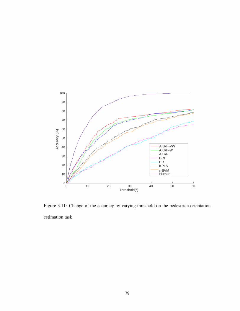
Threshold(°)0 10 20 30 40 50 60

Acc

urac

y (%

)

0

10

20

30

40

50

60

70

80

90

100

AKRF-VWAKRF-W AKRFBRFERTKPLSǫ-SVMHuman

Figure 3.11: Change of the accuracy by varying threshold on the pedestrian orientation

estimation task

79

Table 3.5: Results of previously proposed approaches. Note that the performance is mea-

sured differently for the previous approaches as the original discrete annotations are used.

See text for the details. All the results are on the TUD Multiview Pedestrians Dataset [An-

driluka et al., 2010]

Method Accuracy8 Accuracy4

Baltieri et al. [2012] - AWG 65 83

Baltieri et al. [2012] - Max 58 76

Chen et al. [2011] 55 76

Tao and Klette [2013] - FourD1 N/A1 69

Tao and Klette [2013] - FourPedRD2 N/A1 71

Andriluka et al. [2010] - Max 31 N/A

Andriluka et al. [2010] - SVM 42 70

Andriluka et al. [2010] - SVM-adj 35 76

80

Figure 3.12: Example results from AKRF-VW. Red lines indicate ground truth orienta-

tions. Blue lines indicate predicted orientations. The first two rows show successful cases

while the last row shows failure cases. Note that many of the failure cases are due to the

flipping errors.

81

Chapter 4: Fashion Apparel Detection: the Role of Deep Convolutional

Neural Network and Pose-dependent Priors

In this work, we propose a method to detect fashion apparels a person in an image

is wearing or holding. The types of fashion apparels include hat, bag, skirt, etc. Fashion

apparel spotting has recently gained considerable traction. A major reason is due to a

variety of applications that a reliable fashion item spotter can enable. For instance, spotted

fashion items can be used to retrieve similar or identical fashion items from an online

inventory.

Unlike most prior works on fashion apparel spotting which address the task as a spe-

cialization of the semantic segmentation to the fashion domain, we address the problem

as an object detection task where the detection results are given in the form of bounding

boxes. Detection-based spotters are more suitable as (a) bounding boxes suffice to con-

struct queries for the subsequent visual search, (b) it is generally faster and have lower

memory footprint than semantic segmentation, (c) large scale pixel-accurate training data

is extremely hard to obtain, while it is much easier to get training data as bounding boxes,

and (d) detection is done at instance-level while semantic segmentation does not differ-

entiate multiple instances belonging to the same class. To the best of our knowledge, our

work is the first detection-based (as opposed to segmentation-based) fashion item spotting

82

method.

Although any existing object detection method can possibly be applied, the fashion

apparel detection task poses its own challenges such as (a) deformation of clothing is

large, (b) some fashion items classes are extremely similar to each other in appearance

(e.g., skirt and bottom of short dress), (c) the definition of fashion item classes can be

ambiguous (e.g., pants and tights), and (d) some fashion items are very small (e.g., belt,

jewelry). In this work, we address some of these challenges by incorporating state-of-the-

art object detectors with various domain specific priors such as pose, object shape and

size.

The state-of-the-art object detector we employ in this work is R-CNN Girshick et al.

[2014], which combines object proposals with a Convolutional Neural Network Fukushima

[1980], Lecun et al. [1998]. The R-CNN starts by generating a set of object proposals in

the form of bounding boxes. Then image patches are extracted from the generated bound-

ing boxes and resized to a fixed size. The Convolutional Neural Network pretrained on

a large image database for the image classification task is used to extract features from

each image patch. SVM classifiers are then applied to each image patch to determine if

the patch belongs to a particular class. The R-CNN is suitable for our task as it can detect

objects with various aspect ratios and scales without running a scanning-window search,

reducing the computational complexity as well as false positives.

It is evident that there are rich priors that can be exploited in the fashion domain. For

instance, handbag is more likely to appear around the wrist or hand of the person holding

them, while shoes typically occur near feet. The size of items are typically proportional

to the size of a person. Belts are generally elongated. One of our contributions is to

83

integrate these domain-specific priors with the object proposal-based detection method.

These priors are learned automatically from the training data.

We evaluate the detection performance of our algorithm on the previously intro-

duced Fashionista dataset Yamaguchi et al. [2012] using a newly created set of bounding

box annotations. We convert the segmentation results of state-of-the-art fashion item spot-

ter into bounding box results and compare with the results of the proposed method. The

experiments demonstrate that our detection-based approach outperforms the state-of-the

art segmentation-based approaches in mean Average Precision criteria.

The rest of the chapter is organized as follows. Section 4.1 summarizes related

work in fashion item localization. Our proposed method is detailed in Section 4.2 where

we start with object proposal, followed by classification of these proposals using a com-

bination of generative and discriminative approaches. Section 4.3 validates our approach

on the popular Fashionista Dataset Yamaguchi et al. [2012] by providing both qualitative

and quantitative evaluations. Finally, Section 4.4 contains closing remarks.

4.1 Related Work

The first segmentation-based fashion spotting algorithm for general fashion items

was proposed by Yamaguchi et al. [2012] where they introduce the Fashionista Dataset

and utilize a combination of local features and pose estimation to perform semantic seg-

mentation of a fashion image. In Yamaguchi et al. [2013], the same authors followed up

this work by augmenting the existing approach with data driven model learning, where a

model for semantic segmentation was learned only from nearest neighbor images from an

84

Figure 4.1: Bounding boxes of three different instances of “skirt” class. The aspect ratios

vary significantly even though they are from the same object class.

external database. Further, this work utilizes textual content along with image informa-

tion. The follow up work reported considerably better performance than the initial work.

We report numbers by comparing to the results accompanying these two papers.

Apart from the above two works, Hasan and Hogg [2010] also proposed a segmentation-

based approach aimed at assigning a unique label from “Shirt”, “Jacket”, “Tie” and “Face

and skin” classes to each pixel in the image. Their method is focused on people wearing

suits.

There exist several clothing segmentation methods Gallagher and Chen [2008], Hu

et al. [2008], Wang and Ai [2011] whose main goal is to segment out the clothing area

in the image and types of clothing are not dealt with. In Gallagher and Chen [2008],

a clothing segmentation method based on graph-cut was proposed for the purpose of

identity recognition. In Hu et al. [2008], similar to Gallagher and Chen [2008], a graph-

85

cut based method was proposed to segment out upper body clothing. Wang and Ai [2011]

presented a method for clothing segmentation of multiple people. They propose to model

and utilize the blocking relationship among people.

Several works exist for classifying types of upper body clothing Bossard et al.

[2012], Shen et al. [2014], Chen et al. [2012]. In Shen et al. [2014], a structured learning

technique for simultaneous human pose estimation and garment attribute classification is

proposed. The focus of this work is on detecting attributes associated with upper body

clothing, such as collar types, color, types of sleeves, etc. Similarly, an approach for de-

tecting apparel types and attributes associated with upper bodies was proposed in Bossard

et al. [2012], Chen et al. [2012]. Since localization of upper body clothing is essentially

solved by upper body detectors and detecting upper body is relatively easy, the focus of

the above methods has been on subsequent classification stage. On the other hand, we

focus on a variety of fashion items with various sizes which cannot be easily detected

even with perfect pose information.

Yang and Yu [2011] proposed a real-time clothing recognition method in surveil-

lance settings. They first obtain foreground segmentation and classify upper bodies and

lower bodies separately into a fashion item class. In Bourdev et al. [2011], a poselet-

based approach for human attribute classification is proposed. In their work, a set of

poselet detectors is trained and for each poselet detection, attribute classification is done

using SVM. The final results are then obtained by considering the dependencies between

different attributes. In Wang and Cottrell [2015], recognition of social styles of people

in an image is addressed by Convolutional Neural Network applied to each person in the

image as well as the entire image.

86

Object Proposal

Feature Extraction

SVM for Class 1

SVM for Class K

Geometric Priors NMS

Geometric Priors NMS

Input Image

Bounding Boxes Final

Result

Pose Prediction

Predicted Pose

Hat

Shorts

Bag

Figure 4.2: Overview of the proposed algorithm for testing stage. Object proposals are

generated and features are extracted using Deep CNN from each object proposal. An

array of 1-vs-rest SVMs are used to generate appearance-based posteriors for each class.

Geometric priors are tailored based on pose estimation and used to modify the class prob-

ability. Non-maximum suppression is used to arbitrate overlapping detections with ap-

preciable class probability.

4.2 Proposed Method

The aim of the proposed method is to detect fashion items in a given image, worn

or carried by a single person. The proposed method can be considered as an extension

of the recently proposed R-CNN framework Girshick et al. [2014], where we utilize var-

ious priors on location, size and aspect ratios of fashion apparels, which we refer to as

geometric priors. Specifically for location prior, we exploit strong correlations between

the pose of the person and location of fashion items. We refer to this as pose context.

We combine these priors with an appearance-based posterior given by SVM to obtain the

final posterior density function. Thus, the model we propose is a hybrid of discriminative

and generative models.

The recognition pipeline of the proposed algorithm for the testing stage is shown in

87

Figure 4.2. First, the pose of the person is estimated by an off-the-shelf pose estimator.

Then, a set of candidate bounding boxes is generated by an object proposal algorithm. Im-

age features are extracted from the contents of each bounding box. These image features

are then fed into a set of SVMs with a sigmoid function to obtain an appearance-based

posterior for each class. By utilizing the geometric priors, the final posterior probability

for each class is computed for each bounding box. The results are then filtered by a stan-

dard non-maximum suppression method by Felzenszwalb et al. [2010]. We present the

details of each component below.

4.2.1 Object Proposal

Object detection based on a sliding window strategy has been a standard approach Felzen-

szwalb et al. [2010], Dalal and Triggs [2005], Viola and Jones [2001], Bourdev and Malik

[2009] where object detectors are exhaustively run on all possible locations and scales of

the image. To accommodate the deformation of objects, most recent works detect a sin-

gle object by a set of part-specific detectors and allow the configurations of the parts to

vary. Although a certain amount of deformation is accommodated, possible aspect ratios

considered are still limited and the computation time increases linearly as the number of

part detectors increases.

In our task, the intra-class shape variation is large. For instance, as shown in Figure

4.1, bounding boxes of three instances from the same “skirt” class have very different

aspect ratios. Thus, for practical use, detection methods which can accommodate various

deformations without significant increase in computation time are required.

88

In order to address these issues, we use object proposal algorithms Uijlings et al.

[2013], Arbelaez et al. [2014] employed by state-of-the-art object detectors (i.e., R-CNN

Girshick et al. [2014]). The object proposal algorithm generates a set of candidate bound-

ing boxes with various aspect ratios and scales. Each bounding box is expected to contain

a single object and the classifier is applied only at those candidate bounding boxes, re-

ducing the number of false positives. For the classification step, an image patch within

a bounding box is resized to a predefined size and image features are extracted. Since

feature computation is done only at the generated bounding boxes, the computation time

is significantly reduced while allowing various aspect ratios and scales. In this work, we

employ Selective Search (SS) Uijlings et al. [2013] as the object proposal method.

4.2.2 Image Features by CNN

Our framework is general in terms of the choice of image features. However, re-

cent results in the community indicate that features extracted by Convolutional Neural

Network (CNN) Fukushima [1980], Lecun et al. [1998] with many layers perform signif-

icantly better than the traditional hand-crafted features such as HOG and LBP on various

computer vision tasks Farabet et al. [2012], Krizhevsky et al. [2012], Sermanet et al.

[2013], Zhang et al. [2014]. However, in general, to train a good CNN, a large amount of

training data is required.

Several papers have shown that features extracted by CNN pre-trained on a large

image dataset are also effective for other vision tasks. Specifically, a CNN trained on Im-

ageNet database Deng et al. [2009] is used for various related tasks as a feature extractor

89

and achieve impressive performance Donahue et al. [2014], Razavian et al. [2014]. In

this work, we use CaffeNet Jia et al. [2014] trained on ImageNet dataset as the feature

extractor. We use a 4096 dimensional output vector from the second last layer (fc7) of

CaffeNet as a feature vector.

4.2.3 SVM training

For each object class, we train a linear SVM to classify an image patch as positive

or negative. The training patches are extracted from the training data with ground-truth

bounding boxes. The details of the procedure are described in Section 4.3.2.

4.2.4 Probabilistic formulation

We formulate a probabilistic model to combine outputs from the SVM and the priors

on the object location, size and aspect ratio (geometric priors) into the final posterior for

each object proposal. The computed posterior is used as a score for each detection.

Let B = (x1, y1, x2, y2) denote the bounding box coordinates of an object proposal.

Let f denote the image features extracted from B. We denote by c = (lx, ly) the location

of the bounding box center, where lx = (x1 + x2)/2 and ly = (y1 + y2)/2. We denote

by a = log((y2 − y1)/(x2 − x1)), the log aspect ratio of the bounding box and by r =

log((y2− y1) + (x2−x1)) the log of half the length of the perimeter of the bounding box.

We refer to c, a and r as geometric features.

Let Y denote a set of fashion item classes and yz ∈ {+1,−1} where z ∈ Y , denote

a binary variable indicating whether or not B contains an object belonging to z. Let

90

t = (t1, . . . , tK) ∈ R2×K denote pose information, which is a set of K 2D joint locations

on the image. The pose information serves as additional contextual information for the

detection.

We introduce a graphical model describing the relationship between the above vari-

ables and define a posterior of yz given f , t, c, a and r as follows:

p(yz|f, c, a, r, t) ∝ p(yz|f)p(c|yz, t)p(a|yz)p(r|yz, t) (4.1)

Here we assume that p(t) and p(f) are constant. The first term on the RHS of Eq. 4.1

defines the appearance-based posterior and the following terms are the priors on the ge-

ometric features. For each object proposal, we compute p(yz = 1|f, c, a, r, t) and use it

as a detection score. The introduced model can be seen as a hybrid of discriminative and

generative models. In the following sections, we give the details of each component.

4.2.5 Appearance-based Posterior

We define an appearance based posterior p(yz = 1|f) as

p(yz = 1|f) = Sig(wTz f ;λz) (4.2)

where wz is an SVM weight vector for the class z and λz is a parameter of the sigmoid

function Sig(x;λz) = 1/(1 + exp(−λzx)). The parameter λz controls the shape of the

sigmoid function. We empirically find that the value of λz largely affects the performance.

We optimize λz based on the final detection performance on the validation set.

91

4.2.6 Geometric Priors

Priors on Aspect Ratio and Perimeter

The term p(r|yz = 1, t) is the prior on perimeter conditioned on the existence of an

object from class z and pose t. Intuitively, the length of perimeter r, which captures the

object size, is useful for most of the items as there is a typical size for each item. Also,

r is generally proportional to the size of a person. The size of the person can be defined

using t in various ways. However, in this work, since the images in the dataset we use for

experiments are already normalized such that the size of the person is roughly same, we

assume p(r|yz = 1, t) = p(r|yz = 1).

The term p(a|yz = 1) is the prior on the aspect ratio of object bounding box condi-

tioned on the existence of an object from class z. Intuitively, the aspect ratio a is useful

for detecting items which have a distinct aspect ratio. For instance, the width of waist

belt and glasses are most likely larger than their height. To model both p(a|yz = 1) and

p(r|yz = 1), we use a 1-D Gaussian fitted by standard maximum likelihood estimation.

Pose dependent prior on the bounding box center

We define a pose dependent prior on the bounding box center as

p(c|yz = 1, t) = Πk∈Tzp(lx, ly|yz = 1, tk) (4.3)

= Πk∈Tzp((lx, ly)− tk|yz = 1) (4.4)

where Tz is a set of joints that are informative about the bounding box center location of

the object belonging to the class z. The algorithm to determine Tz for each fashion item

92

−300 −200 −100 0 100 200 300−400

−350

−300

−250

−200

−150

−100

−50

0

(a) Bag - Neck

−300 −200 −100 0 100 200 300−200

−150

−100

−50

0

50

100

150

(b) Left Shoe - Left Ankle

Figure 4.3: Distributions of relative location of item with respect to location of key joint.

Key joint location is depicted as a red cross. (a) distribution of relative location of bag with

respect to neck is multi-modal. (b) locations of left shoe and left ankle are strongly cor-

related and the distribution of their relative location has a single mode. See Section 4.2.6

for details.

class z will be described shortly. Each p((lx, ly)− tk|yz = 1) models the relative location

of the bounding box center with respect to the k-th joint location.

Intuitively, the locations of fashion items and those of body joints have strong cor-

relations. For instance, the location of hat should be close to the location of head and thus,

the distribution of their offset vector, p((lx, ly)−tHead|yHat = 1) should have a strong peak

around tHead and relatively easy to model. On the other hand, the location of left hand is

less informative about the location of the hat and thus, p((lx, ly)− tLefthand|yHat = 1) has

a complex distribution which is difficult to model accurately. Thus, it is beneficial to use

for each fashion item only a subset of body joints that have strong correlations with the

location of that item.

93

The relative location of the objects with respect to the joints can be most faithfully

modeled as a multimodal distribution. For instance, bags, purses and wallets are typ-

ically carried on either left or right hand side of the body, thus generating multimodal

distributions. To confirm this claim, In Figure 4.3, we show a plot of (lx, ly) − tNeck of

“Bag” and a plot of (lx, ly) − tLeftAnkle of “Left Shoe” obtained from the dataset used in

our experiments. As can be seen, p((lx, ly) − tNeck|yBag = 1) clearly follows a multi-

modal distribution while p((lx, ly)− tLeftAnkle|yLeftShoe = 1) has a unimodal distribution.

Depending on the joint-item pair, it is necessary to automatically choose the number of

modes.

To address the challenges raised above, we propose an algorithm to automatically

identify the subset of body joints Tz and learn a model. For each pair of a fashion item z

and a body joint k, we model p((lx, ly)−tk|yz = 1) by a Gaussian mixture model (GMM)

and estimate the parameters by the EM-algorithm. We determine the number of GMM

components based on the Bayesian Information Criteria Kashyap [1977], Schwarz [1978]

to balance the complexity of the model and fit to the data. To obtain Tz for item z, we

pick the top 2 joints whose associated GMM has larger likelihood. This way, for each

item, body joints which have less scattered offsets are automatically chosen. The selected

joints for each item will be shown in the next section.

94

4.3 Experiments

4.3.1 Dataset

To evaluate the proposed algorithm, we use the Fashionista Dataset which was in-

troduced by Yamaguchi et al. [2012] for pixel-level clothing segmentation. Each image

in this dataset is fully annotated at pixel level, i.e. a class label is assigned to each pixel.

In addition to pixel-level annotations, each image is tagged with fashion items presented

in the images. In Yamaguchi et al. [2013], another dataset called Paper Doll Dataset in-

cluding 339,797 tagged images is introduced and utilized to boost performance on the

Fashionista Dataset. Our method does not use either associated tags or the Paper Doll

Dataset. We use the predefined training and testing split for the evaluation (456 images

for training and 229 images for testing) and take out 20% of the training set as the valida-

tion set for parameter tuning.

In the Fashionista Dataset, there are 56 classes including 53 fashion item classes and

three additional non-fashion item classes (hair, skin and background.) We first remove

some classes that do not appear often in the images and those whose average pixel size is

too small to detect. We then merge some classes which look very similar. For instance,

there are “bag”, “Purse” and “Wallet” classes but the distinction between those classes

is visually vague, thus we merge those three classes into a single ”Bag” class. We also

discard all the classes related to footwear such as “sandal” and “heel’ and instead add “left

shoe” and “right shoe” classes which include all types of footwear. It is intended that, if

needed by a specific application, a sophisticated fine-grained classification method can be

95

applied as a post-processing step once we detect the items. Eventually, we obtain 10 new

classes where the occurrence of each class is large enough for training the detector and

the appearance of items in the same class is similar. The complete definition of the new

ten classes and some statistics are shown in Table 4.1.

We create ground-truth bounding boxes based on pixel-level annotations under the

new definition of classes. For classes other than “Left shoe” and “Right shoe”, we de-

fine a ground-truth bounding box as the one that tightly surrounds the region having the

corresponding class label. For “Left shoe” and “Right shoe” classes, since there is no

distinction between right and left shoes in the original pixel-level annotations, this au-

tomatic procedure cannot be applied. Thus, we manually annotate bounding boxes for

“Right shoe” and “Left shoe” classes. These bounding box annotation are available at the

author’s website to facilitate further research on fashion apparel detection.

Our framework is general in the choice of pose estimators. In this work, we use

pose estimation results provided in the Fashionista Dataset, which is based on Yang and

Ramanan [2011]. There are 14 key joints namely head, neck, left/right shoulder, left/right

elbow, left/right wrist, left/right hip, left/right knee and left/right foot.

In Table 4.1, we show the first and second key body joints that are selected by the

proposed algorithm. Interestingly, for “Pants”, “Shorts” and “Skirt”, left hip and right hip

are selected but for “Tights”, left knee and right knee are selected instead.

96

4.3.2 Detector Training

We create image patches for training the detector by cropping the training images

based on corresponding ground-truth bounding box. Before cropping, we enlarge the

bounding boxes by a scale factor of 1.8 to include the surrounding regions, thus providing

contextual information. Note that we intentionally make the contextual regions larger than

Girshick et al. [2014] as contextual information would be more important when detecting

small objects like fashion items we consider in this work. The cropped image patches are

then resized to the size of the first layer of CaffeNet (227 by 227 pixels). To increase the

number of training patches, we run the object proposal algorithm on the training images

and for each generated bounding box, we compute the intersection over union (IoU) with

the ground-truth bounding boxes. If the IoU is larger than 0.5 for a particular class, we

use the patch as an additional training instance for that class. If IoU is smaller than 0.1

with ground-truth bounding boxes of all the classes, we use it as a training instance for

the background class. We also obtain the training patches for the background class by

including image patches from ground-truth bounding boxes of the classes which we do

not include in our new ten classes.

The number of training patches for each class obtained is shown in Table 4.3. From

the obtained training patches, we train a set of linear SVMs, each of which is trained by

using instances in a particular class as positive samples and all instances in the remaining

classes as negative samples. The parameters of SVMs are determined using the validation

set.

97

4.3.3 Baseline Methods

Since fashion apparel detection has not been previously addressed, there is no ex-

isting work proposed specifically for this task. Thus, we convert the pixel-level segmen-

tation results of Yamaguchi et al. [2012] and Yamaguchi et al. [2013] to bounding boxes

and use their performance as baselines. To obtain bounding boxes from segmentation

results, we use the same procedure we use to generate ground-truth bounding boxes from

the ground-truth pixel-level annotations. Note that we exclude “Left shoe” and “Right

shoe” from the comparison since in their results, there is no distinction between left and

right shoes.

4.3.4 Results

We first evaluate the performance of the object proposal methods in terms of preci-

sion and recall. Here, precision is defined as the number of object proposals which match

the ground-truth bounding boxes regardless of class, divided by the total number of object

proposals. Specifically, we consider each object proposal as correct if IoU ≥ 0.5 for at

least one ground-truth bounding box. We compute recall for each class by the number

of ground-truth bounding boxes which have at least one corresponding object proposal,

divided by the total number of ground-truth bounding boxes.

In Table 4.4, we show the precision, recall and the average number of object propos-

als per image. We tune the parameters of both object proposal algorithms to retain high

recall so that it will not miss too many true objects. Although it results in low precision,

false positives are reduced in the subsequent classification stage.

98

We evaluate the performance of the detection methods using the average preci-

sion (AP) computed from the Precision-Recall curves. In Table 4.2, we report the per-

formance of the proposed framework with three different settings, “Full” represents our

complete method using both geometric priors and appearance-based posterior, “w/o ge-

ometric prior” represents a method which excludes the geometric priors from “Full” and

“w/o appearance” is a method which excludes appearance-based posterior from “Full”.

From the comparison between “Full” and “w/o geometric prior”, it is clear that

incorporating geometric priors significantly improves the performance (35.8% improve-

ment for mAP). This result indicates the effectiveness of the geometric priors in the fash-

ion item detection task.

In Figure 4.4 we show the precision-recall curves of the proposed methods with

various settings as well as precision-recall points of the baseline methods. In the figures,

“paperdoll” refers to the results of Yamaguchi et al. [2013] and “fashionista” refers to

Yamaguchi et al. [2012]. Except for “Pants”, our complete method outperforms the base-

lines with a large margin. Note that “paperdoll” Yamaguchi et al. [2013] uses a large

database of tagged fashion images as additional training data.

In Figure 4.5, we show some qualitative results. Figure 4.6 shows sample images

where our approach makes mistakes. We see that fashion apparel detection has its own

unique challenges. First of all, even with our new fashion item classes, some fashion items

are visually very similar to each other. For example, “Tights” and “Pants” can look very

similar since both items can have a variety of colors. The only distinguishable cue might

be how tight it is, which is quite challenging to capture. Another example is “Skirt” and

bottom half of a dress. Both items have extremely similar appearance. The only difference

99

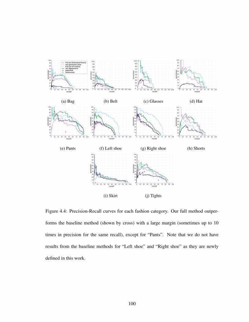
0 10 20 30 40 50 60 70 80 90 1000

10

20

30

40

50

60

70

80

90

100

recall

pre

cisi

on

Full (w/ Estimated Poses)w/o geometric priorFull (w/ GT Poses)w/o appearancepaperdollfashionista

(a) Bag

0 10 20 30 40 50 60 70 80 90 1000102030405060708090

100

recallp

reci

sion

(b) Belt

0 10 20 30 40 50 60 70 80 90 1000102030405060708090

100

recall

pre

cisi

on

(c) Glasses

0

10

20

30

40

50

60

70

80

90

100

pre

cisi

on

0 10 20 30 40 50 60 70 80 90 100recall

(d) Hat

0

10

20

30

40

50

60

70

80

90

100

pre

cisi

on

0 10 20 30 40 50 60 70 80 90 100recall

(e) Pants

0

10

20

30

40

50

60

70

80

90

100

pre

cisi

on

0 10 20 30 40 50 60 70 80 90 100recall

(f) Left shoe

0

10

20

30

40

50

60

70

80

90

100

pre

cisi

on

0 10 20 30 40 50 60 70 80 90 100recall

(g) Right shoe

0

10

20

30

40

50

60

70

80

90

100

pre

cisi

on

0 10 20 30 40 50 60 70 80 90 100recall

(h) Shorts

0

10

20

30

40

50

60

70

80

90

100

pre

cisi

on

0 10 20 30 40 50 60 70 80 90 100recall

(i) Skirt

0

10

20

30

40

50

60

70

80

90

100

pre

cisi

on

0 10 20 30 40 50 60 70 80 90 100recall

(j) Tights

Figure 4.4: Precision-Recall curves for each fashion category. Our full method outper-

forms the baseline method (shown by cross) with a large margin (sometimes up to 10

times in precision for the same recall), except for “Pants”. Note that we do not have

results from the baseline methods for “Left shoe” and “Right shoe” as they are newly

defined in this work.

100

is that a dress is a piece of cloth which covers both upper body and lower body and this

difference is difficult to detect. Furthermore, “Belt” and “Glasses” are difficult to detect

as they are usually very small.

4.4 Conclusion

In this work, we reformulate fashion apparel parsing, traditionally treated as a se-

mantic segmentation task, as an object detection task and propose a probabilistic model

which incorporates state-of-the-art object detectors with various geometric priors of the

object classes. Since the locations of fashion items are strongly correlated with the pose

of a person, we propose a pose-dependent prior model which can automatically select the

most informative joints for each fashion item and learn the distributions from the data.

Through experimental evaluations, we observe the effectiveness of the proposed priors

for fashion apparel detection.

4.5 Acknowledgments

The work presented in this chapter was conducted as part of the summer internship

at eBay Research Labs.

101

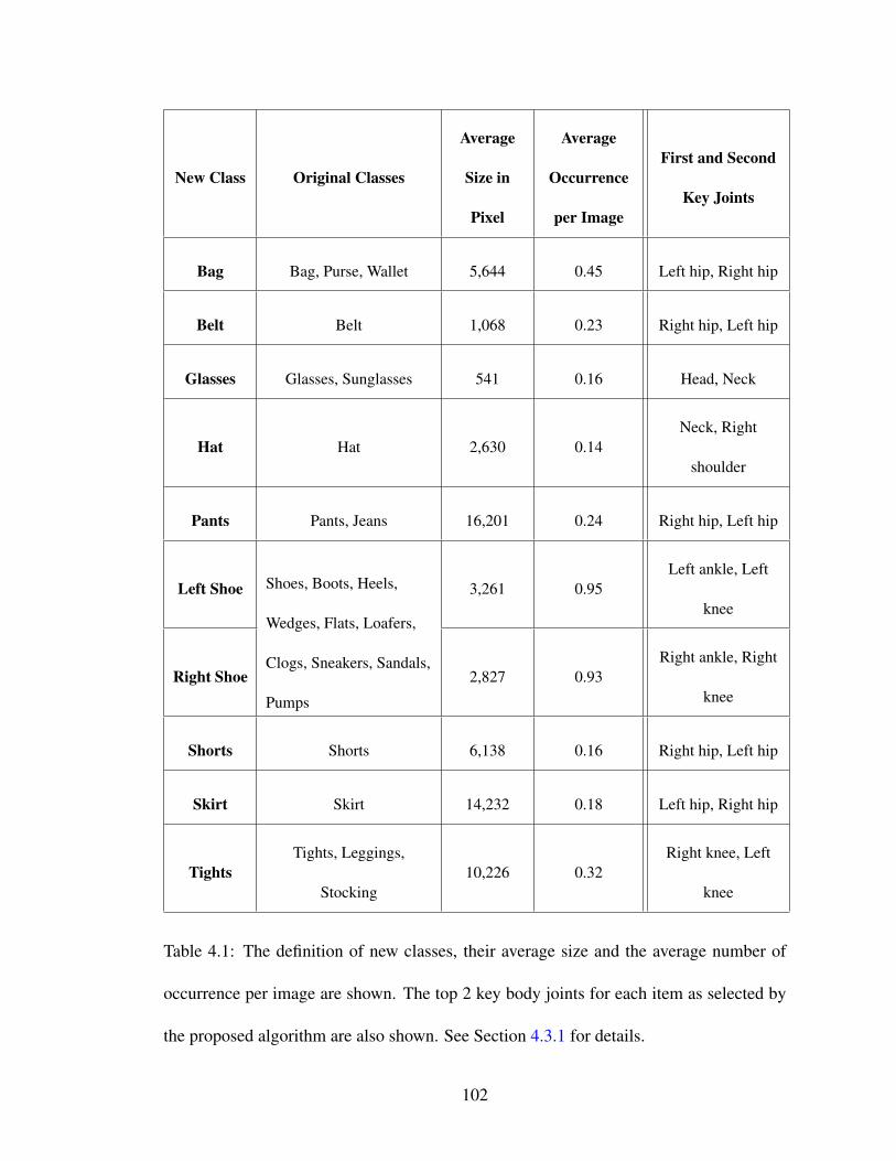
New Class Original Classes

Average

Size in

Pixel

Average

Occurrence

per Image

First and Second

Key Joints

Bag Bag, Purse, Wallet 5,644 0.45 Left hip, Right hip

Belt Belt 1,068 0.23 Right hip, Left hip

Glasses Glasses, Sunglasses 541 0.16 Head, Neck

Hat Hat 2,630 0.14Neck, Right

shoulder

Pants Pants, Jeans 16,201 0.24 Right hip, Left hip

Left Shoe Shoes, Boots, Heels,

Wedges, Flats, Loafers,

Clogs, Sneakers, Sandals,

Pumps

3,261 0.95Left ankle, Left

knee

Right Shoe 2,827 0.93Right ankle, Right

knee

Shorts Shorts 6,138 0.16 Right hip, Left hip

Skirt Skirt 14,232 0.18 Left hip, Right hip

TightsTights, Leggings,

Stocking10,226 0.32

Right knee, Left

knee

Table 4.1: The definition of new classes, their average size and the average number of

occurrence per image are shown. The top 2 key body joints for each item as selected by

the proposed algorithm are also shown. See Section 4.3.1 for details.

102

Methods mAP Bag Belt Glasses Hat PantsLeft

Shoe

Right

ShoeShorts Skirt Tights

Full 31.1 22.5 14.2 22.2 36.1 57.0 28.5 32.5 37.4 20.3 40.6

w/o geo-

metric

priors

22.9 19.4 6.0 13.0 28.9 37.2 20.2 23.1 34.7 15.2 31.7

w/o ap-

pearance17.8 4.3 7.1 7.5 8.9 50.7 20.5 23.4 15.6 18.0 22.3

Table 4.2: Average Precision of each method. “Full” achieves better mAP and APs for all

the items than “w/o geometric priors” and “w/o appearance”.

Bag Belt Glasses Hat PantsLeft

shoe

Right

shoeShorts Skirt Tights Background

1,254 318 177 306 853 1,799 1,598 473 683 986 225,508

Table 4.3: The number of training patches generated for each class with Selective

Search Uijlings et al. [2013].

103

Precision

(%)

Recall (%) Avg. # of

bounding

boxesAvg. Bag Belt Glasses Hat PantsLeft

shoe

Right

shoeShorts Skirt Tights

1.36 86.7 93.6 69.2 62.5 95.3 93.6 86.6 82.4 93.2 98.8 91.2 1073.4

Table 4.4: Precision, recall and the average number of generated bounding boxes per

image. Note that it is important to have high recall and not necessarily precision so that

we will not miss too many true objects. Precision is controlled later by the classification

stage.

104

shorts

tights

Left Shoe Right Shoe Right Shoe

Right Shoe

Right Shoe

Right Shoe

Right Shoe

Ri ht ShLeft Shoe Left Shoe

ShoeLeft Shoe

Left Shoe

pants pants

bag

bag

bag

glasses

hat

hat

belt

shorts

skirt

skirt

tights

Figure 4.5: Example detection results obtained by the proposed method. Note that we

manually overlaid the text labels to improve legibility.

105

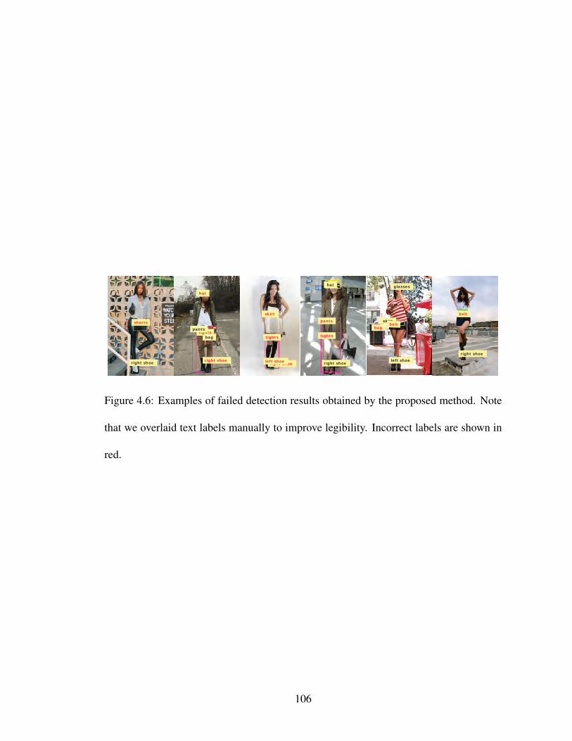
hatglasses

right shoe right shoe

right shoeright shoeright shoe left shoeleft shoe

belt

hat

bag

bag

skirtbelt

skirt

shorts

tightstightstights

pants

pants

Figure 4.6: Examples of failed detection results obtained by the proposed method. Note

that we overlaid text labels manually to improve legibility. Incorrect labels are shown in

red.

106

Chapter 5: Attentional Network for Visual Object Detection

Object detection is one of the most fundamental problems in computer vision.

Given an image, the goal of an object detection algorithm is to detect and localize all

instances of pre-defined object classes, typically in the form of bounding boxes with con-

fidence values. Although an object detection problem can be converted to many object

classification problems by a scanning window technique [Viola and Jones, 2004], it is

inefficient since a classifier has to be applied to all potential image regions at various lo-

cations, scales, and aspect ratios. The region-based convolution neural network (R-CNN)

[Girshick et al., 2014] algorithm suggested recently a two-stage approach. It first gener-

ates a set of object proposals, called regions of interest (ROI), using a proposal generator

and then determines the existence of an object and its classes in the ROI using a deep

neural network. The R-CNN algorithm has achieved impressive performance on public

benchmarks and has become the backbone of many recent object detection methods.

In detecting an object, the R-CNN algorithm and its extensions look at the ROI (and

sometimes its neighborhood) given by the proposal generator only once. This is in con-

trast to humans’ capability of multiple fixations of visual attention as depicted in Fig. 5.1.

We propose to imitate such an attention mechanism for improving the object detection

performance of the R-CNN algorithm. To this end, we develop an algorithm that adap-

107

tively places a sequence of glimpses for accumulating visual evidence for determining

the object class and its precise location from ROIs. We use a recurrent neural network for

learning the glimpse placement as well as for summarizing the visual evidence extracted

from the multiple glimpse. Due to lacks of ground truth annotations of visual attention for

the object detection task, we use a reinforcement algorithm to train the proposed network.

Our work is largely inspired by Mnih et al. [2014a], which uses a visual attention

mechanism for the handwritten digit classification task. In this chapter, we study a more

challenging task, detecting visual objects in images. Due to large variation in object ap-

pearances, it is more difficult to learn a reliable attention mechanism. The glimpse has

to vary both in shapes and scales for finding most relevant information. We investigate

the network structure that can facilitate the learning of a reliable visual attention strategy

for the object detection task. We provide detailed performance analysis in the experi-

ment section. We evaluate the proposed algorithm, which we refer to as Attention-based

visual Object Detection network (AOD), on the PASCAL VOC detection benchmarks

and demonstrate its advantage over the baseline R-CNN algorithm that does not have the

visual attention mechanism.

5.1 Related Work

The attention mechanism has been proposed for different applications including

speech recognition [Chorowski et al., 2015], machine translation [Bahdanau et al., 2015]

and question–answering [Sukhbaatar et al., 2015]. Among many previous attempts, our

work is inspired by Mnih et al. [2014b] who present a recurrent neural network model that

108

sequentially selects and processes sub-regions of an image and combines the information

from those regions to obtain a better representation for a targeted task. The method is ap-

plied to classify handwritten digit images with clutters, and excellent results are demon-

strated. The proposed method is an extension of Mnih et al. [2014b] to the more difficult

visual object detection task for dealing with variations in appearances deformations and

scales. Unlike the classification task, the object detection task requires algorithms to lo-

calize multiple objects from various classes present in an input image. While in Mnih

et al. [2014b], glimpse size and shape are fixed, in our method, glimpse can change its

shape adaptively to detect objects in various size and shapes.

A lot of works have been done on various vision tasks after Mnih et al. [2014b].

To handle multiple objects in a more realistic image, Ba et al. [2015] extends Mnih et al.

[2014b] by allowing a model to predict one object at each time step, making the glimpse

network deeper and introducing a context network. The method is applied to the task of

transcribing multi-digit house numbers from Google Street View images. Sermanet et al.

[2015] applies a recurrent neural network almost identical to the one in Ba et al. [2015]

to a more challenging fine-grained categorization task. Yeung et al. [2015] also uses a

recurrent neural network trained by the REINFORCE algorithm to address a video-based

action detection task and achieves state-of-the-art results. Unlike Mnih et al. [2014b], Ba

et al. [2015], Sermanet et al. [2015] where a spatial attention policy is learned, a model

in Yeung et al. [2015] learns to output temporal attentions. Beside the aforementioned

works, a recurrent neural network with an attention mechanism trained by a reinforcement

learning algorithm has been applied to tasks such as image caption generation [Xu et al.,

2015], image generation [Gregor et al., 2015] and action recognition [Sharma et al., 2015].

109

A few attention-based methods have been proposed for the object detection task.

Caicedo and Lazebnik [2015] train a class specific object localization model using a rein-

forcement learning technique and utilize the model for a detection task by evaluating all

the regions generated over the course of localization. Yoo et al. [2015] also propose a class

specific model which iteratively modifies the initial ROI until it declares the existence of

an object. Unlike these works, the proposed method is class agnostic, which scales better

with the number of object classes as we do not need to train a separate detector for each

object class.

Most of the recent object detection methods are following the R-CNN style ap-

proach. There are currently two main directions explored for further improvement. The

first direction is to make the underlying CNN deeper [He et al., 2015]. The second one is

incorporating semantic segmentation [Dai et al., 2015], which typically require additional

training data for semantic segmentation. Other works focus on speeding up the computa-

tion time [Girshick, 2015, Ren et al., 2015, Redmon et al., 2015, Lenc and Vedaldi, 2015,

Najibi et al., 2015].

An attempt to extract features from multiple regions is made by a few works. In

Gidaris and Komodakis [2015], in addition to the proposal bounding box, visual features

are extracted from a set of hand-crafted regions and used for the recognition. Bell et al.

[2015] also explore the use of multiple regions by extracting features from the entire

image in addition to the proposal bounding boxes in order to capture the context. Unlike

ours, the additional regions are manually predefined and not adaptively selected.

110

5.2 Attention-based Object Detection Network

Figure 5.1: Humans have the capability of using multiple fixation points to accumulate

evidences for detecting objects in a scene.

We describe the AOD network in details. The network is a deep recurrent neural

network designed to detect objects in an image by placing a sequence of glimpses of

different sizes and aspect ratios, and make a final decision based on features extracted

from these glimpses. Each sequence starts from an object proposal bounding box given

by the proposal generator and at the end of the sequence, the network produces scores

and bounding boxes for all of the pre-defined classes. With the help of a reinforcement

learning algorithm, the network is trained to generate glimpses that lead to better detection

performance. In the following, we first describe our network behavior in the test time,

then we briefly introduce the reinforcement algorithm and the training procedure for the

proposed network.

5.2.1 Network Architecture

The AOD network illustrated in Fig. 5.2 is an active recurrent neural network that

decides the attention areas by itself. Given an image, the detection process starts by first

applying a deep convolutional neural network to the whole image to obtain a set of feature

111

fc6

Bounding box Object class

fc7

Element-wise max operation

t = 1 t = 2 t =T

ROI pooling

Proposal Glimpse

fc7

fc6

ROI pooling

fc7

fc6

ROI pooling

Glimpse

fc7

fc6

ROI pooling

Glimpse

t = 3 Image

Conv 1

Conv 5

Figure 5.2: Illustration of the AOD network: the network consists a stacked recurrent mod-

ule designed for object class recognition, bounding box regression and glimpse generation. The

classification and bounding box regression are done only at the final time step while the glimpse

generation is done at all time steps except the last time step. Given an input image, first, a set of

feature maps are computed by the Deep Convolutional Neural Network. Given a proposal bound-

ing box at t = 1, a fixed dimensional feature vector is extracted from the proposal bounding box

on the last feature map by the ROI pooling layer [Girshick, 2015]. A few fully connected layers

(fc6 and fc7 in the figure), each followed by a ReLU and dropout layers, are then applied to the

extracted feature vector. From the resultant features, a next glimpse bounding box is determined

by applying a fully connected layer. At t = 2, a feature vector is extracted from the glimpse

bounding box region using the ROI pooling layer. The process is repeated until the last time step

t = T . At the last time step, an element-wise max operation is applied to the final feature vectors

at all time steps and then softmax classification and bounding box regression are conducted.

maps as in the Fast R-CNN algorithm [Girshick, 2015]. In the case of utilizing pre-trained

networks such as the AlexNet [Krizhevsky et al., 2012] or the VGG-Net [Simonyan and

Zisserman, 2015], the feature maps are computed from the last convolutional layers. Con-

currently, a set of proposal bounding boxes is obtained by running a proposal generator.

The AOD processes each proposal bounding box separately by extracting the features

112

from the computed feature maps within the bounding box regions. In the following, we

describe a procedure applied to each proposal bounding box.

We denote a glimpse at each time step t byGt ∈ R4. The first ROI,G1, is a proposal

bounding box given by the proposal generator and the subsequent Gt are dynamically de-

termined by the network by aggregating information acquired so far. As in Girshick et al.

[2014], we employ the scale-invariant and height/width normalized shift parameterization

for Gt by using the proposal bounding box as an anchor bounding box. Specifically,

G = (δx, δy, δw, δh) = (gx − pxpw

,gy − pyph

, loggwpw, log

ghph

)

where (gx, gy, gw, gh) is the center coordinate, width and height of the glimpse bound-

ing box. Similarly, (px, py, pw, ph) represents the proposal bounding box. The glimpse

layer generates (δx, δy, δw, δh) for determining the glimpse bounding box, which is con-

sidered as the glimpse at the next time step. Note that the glimpse bounding boxes are not

necessarily the object bounding boxes which indicate the locations of the objects.

From each Gt, a fixed dimensional feature vector is extracted by applying the ROI

pooling [Girshick, 2015] to the computed feature maps region withinGt. The ROI pooling

works by dividing a given ROI into a predefined grid of sub-windows and then max-

pool the feature values in each sub-window. The pooled features are fed into a stacked

recurrent neural network of two layers, which are termed as fc6 and fc7 respectively.

At the last time step t = T , an element-wise max operation is applied to the last fea-

ture vectors at all time steps to compute the final feature vector. The final feature vector is

fed into a softmax classification layer and a bounding box regression layer for computing

the object class and its location. The softmax classification layer outputs class proba-

113

bilities over K foreground object classes and one background class. The bounding box

prediction layer outputs bounding box prediction for each of the K foreground classes.

We argue that the element-wise max operation retains the most strong signal across

time steps independent of the order of the time steps. The stacked recurrent network

allows alternative paths of information propagation. They are used because of empirical

evidence of superior performance as will be discussed in the experiment section.

5.2.2 Reinforcement learning

The glimpse generation problem can be seen as a reinforcement learning (RL) prob-

lem [Sutton and Barto, 1998, Szepesvari, 2010]. In RL, an agent continually interacts with

an environment by observing the state x ∈ X of the environment and then choosing an

action a ∈ A according to its policy π(a|x), a probabilistic mapping from the state to

actions. Depending on the current state and the chosen action, the agent’s state in the

environment changes to X ′ ∼ P(·|x, a). The agent also receives a real-valued reward

signal r ∼ R(·|x, a).

This interaction might continue for a finite or infinite number of steps. In this work,

we consider a finite number of steps T . The outcome of each T step of interactions is

called an episode, which we denote by ξ.

The goal of an RL agent is to maximize a function of the rewards that it receives.

An example of such a function is the sum of rewards in the episode, which can be written

as

R(ξ) =T∑t=1

rt.

114

R(ξ) is called the return of ξ. The goal of an RL can be stated as finding a policy π which

maximize the expected return J(π)def== Eπ [R(ξ)].

What differentiates RL from supervised learning is that there is no training data

consisting of correct input-output pairs. Instead, the policy should be learned based only

on the scalar reward signal that the agent receives at each time step. This is very appro-

priate for our problem as there is no dataset providing us with proper glimpse proposal,

but on the other hand it is relatively easy to specify whether the new glimpse proposal is

useful for the task of object detection or not.

Among many different approaches to solve an RL problem, in this work we use

the REINFORCE algorithm [Wil, 1992], which is a policy gradient approach [Deisenroth

et al., 2013, Sutton et al., 2000]. Suppose π is parameterized by θ. The policy gradient

algorithm, in its simplest form, changes the policy parameters in the direction of gradient

of J(πθ):

θi+1 ← θi + αi∇J(πθi), (5.1)

for some choice of step size αi > 0.

By using the Gaussian distribution as πθ, the approximate gradients are computed

by generating multiple episodes under the current policy (refer to Wil [1992] for the

derivation):

∇θJ(πθ) ≈1

n

n∑i=1

R(ξ(i))T∑t=1

(a(i)t − θx

(i)t )x

(i)>t

σ2. (5.2)

Since this is a gradient ascent algorithm, it can easily be incorporated into the stan-

dard back propagation neural network training. In fact, our network is trained by back

115

propagating both gradient from reinforcement learning and those from supervised train-

ing.

5.2.3 Network Training

The training data fed to our network is constructed in the same way as that in the R-

CNN algorithm. Each generated proposal bounding box is assigned a class label c∗ among

one background class and K foreground object classes according to the overlaps with the

ground-truth object bounding boxes. The background class is anything not belonging

to any of the foreground classes. Also, given to each of the proposal bounding boxes

is a bounding box target vector encoding the scale-invariant translation and log-space

height/width shift relative to the object proposal as in Eq. 5.1. Note that the bounding

box target vectors for background proposal boxes are not defined and thus not used for

training. The details of the training data construction is presented in Sec. 5.2.4.2.

The final outputs from our network are softmax classification scores and bounding

boxes for all of the pre-defined foreground classes. During training, ground-truth for

them are provided, thus the standard Backpropagation Through Time (BPTT) algorithm

[Werbos, 1990] can be used for training. However, since the locations and shapes of the

glimpses which lead to a higher detection performance are unknown, the BPTT algorithm

cannot be applied to train the glimpse generation layer (an arrow from fc7 to Glimpse

in the figure). To train the glimpse generation layer, we use the REINFORCE algorithm

presented in Sec. 5.2.2.

In our model, the state is the input given to the glimpse module (i.e., the output of

116

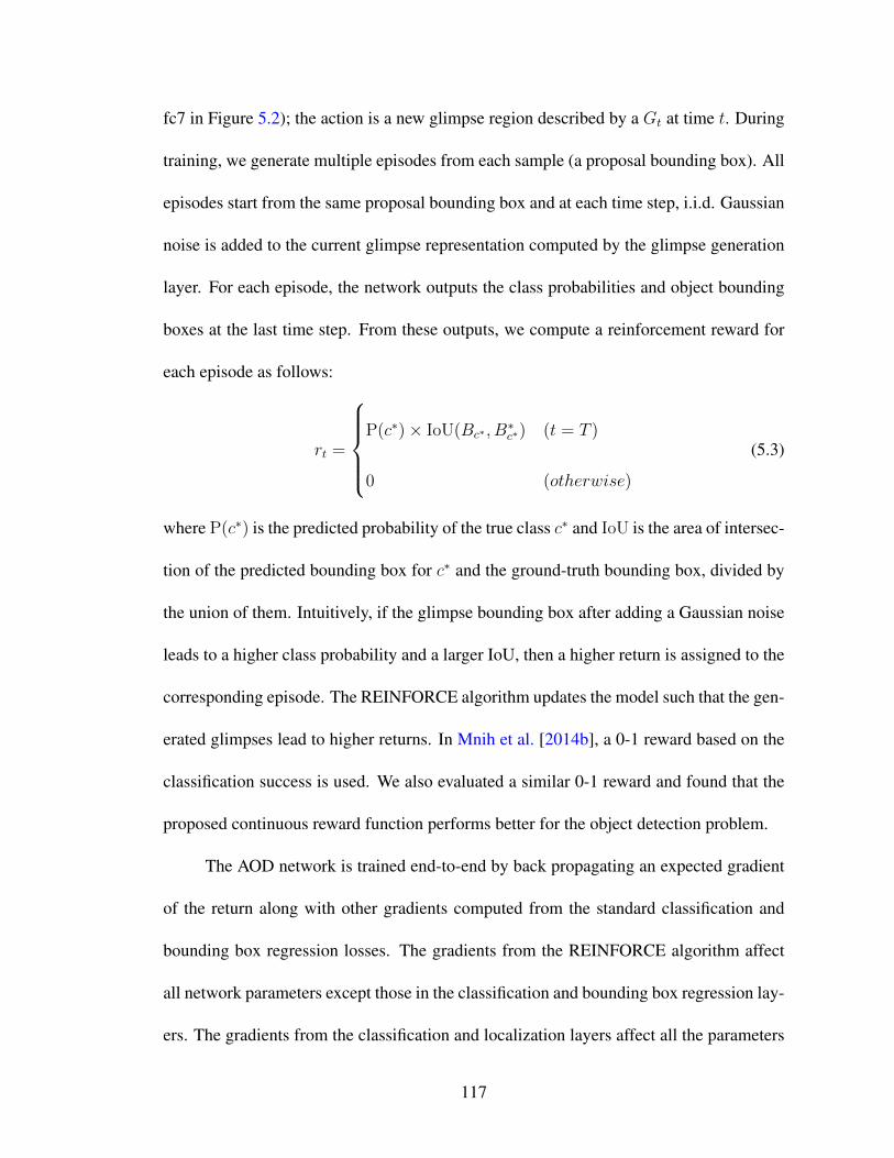
fc7 in Figure 5.2); the action is a new glimpse region described by a Gt at time t. During

training, we generate multiple episodes from each sample (a proposal bounding box). All

episodes start from the same proposal bounding box and at each time step, i.i.d. Gaussian

noise is added to the current glimpse representation computed by the glimpse generation

layer. For each episode, the network outputs the class probabilities and object bounding

boxes at the last time step. From these outputs, we compute a reinforcement reward for

each episode as follows:

rt =

P(c∗)× IoU(Bc∗ , B

∗c∗) (t = T )

0 (otherwise)

(5.3)

where P(c∗) is the predicted probability of the true class c∗ and IoU is the area of intersec-

tion of the predicted bounding box for c∗ and the ground-truth bounding box, divided by

the union of them. Intuitively, if the glimpse bounding box after adding a Gaussian noise

leads to a higher class probability and a larger IoU, then a higher return is assigned to the

corresponding episode. The REINFORCE algorithm updates the model such that the gen-

erated glimpses lead to higher returns. In Mnih et al. [2014b], a 0-1 reward based on the

classification success is used. We also evaluated a similar 0-1 reward and found that the

proposed continuous reward function performs better for the object detection problem.

The AOD network is trained end-to-end by back propagating an expected gradient

of the return along with other gradients computed from the standard classification and

bounding box regression losses. The gradients from the REINFORCE algorithm affect

all network parameters except those in the classification and bounding box regression lay-

ers. The gradients from the classification and localization layers affect all the parameters

117

except those in the glimpse generation layer.

We use the stochastic gradient descent with a mini-batch. To reduce the memory

footprint, one mini-batch contains samples from only a few images. Since the number of

proposal boxes generated by a proposal generator such as the selective search algorithm

[Uijlings et al., 2013] from a single image is large, only a predefined number of fore-

ground samples and background samples are randomly selected and used for training.

The detail is provided in Sec. 5.2.4.3.

The policy gradients are only computed for foreground samples because the appear-

ance variations of the background class is larger than those of the foreground classes and

it is difficult for a reinforcement agent to learn a good glimpse placement policy. The net

effect is that the glimpse generation is optimized only for better discrimination among

foreground objects and more accurate bounding box regression. The benefit of excluding

background samples for the REINFORCE algorithm is evaluated in Sec. 5.4.

5.2.3.1 Return Normalization

In the REINFORCE algorithm, typically a baseline is subtracted from the return in

order to reduce the variance of the expected gradient. A common approach to obtain the

baseline is to use exponential moving average of the return before subtracting the base-

line [Wil, 1992]. Another approach is to learn a value function V (xt) = E[∑T

l=t rl|xt]

and use it as a baseline.

We find out that in our setting, computing reliable baselines is challenging. The

main reason is that our environment is a space of natural images whose variations are

118

significantly large, and the agent is placed into a variety of different image subregions

with different level of difficulties for making accurate decisions. Therefore, it is possible

that all the episodes generated from a proposal bounding box A get higher returns than

those generated from a proposal bounding box B. In this case, all the episodes from A

are prioritized than those from B, which leads to an undesirable training behavior.

To deal with this problem, we convert the original return in Eq. 5.3 by making the

mean and variance of the returns computed from all episodes generated from one sam-

ple to 0 and 1, respectively, and use the converted return in the REINFORCE algorithm.

This way, the new return reflects how well a particular episode works compared to other

episodes from the same sample. Also the new return value is less dependent from the

samples since it is normalized per sample. We find this approach works well in prac-

tice (Sec. 5.4). Note that the proposed return normalization scheme keeps the expected

gradients unbiased as the computed baseline is the expectation over the rewards, which

becomes a constant as computing the expected gradient.

5.2.4 Implementation Details

In this section, we present some of the implementation details.

5.2.4.1 Glimpse features

At each time step, visual features are computed by the ROI pooling based on the

glimpse vector generated in the previous time step. In addition to the visual features, we

use the glimpse vector as an additional feature for the current time step. This is to ensure

119

that the network explicitly knows the glimpses it has produced. One fully connected layer

followed by ReLU is applied to the glimpse vector and concatenated with the last visual

feature vector (i.e., fc7 in Fig. 5.2). Similarly to fc6 and fc7, a recurrent connection is

applied. Note that for t = 1, the zero vector is fed as glimpse features.

5.2.4.2 Training sample construction

The training sample construction follows the procedure described in the Fast R-

CNN algorithm [Girshick, 2015]. For each sample, i.e., proposal bounding box B, we

compute the IoU with all the ground-truth bounding boxes and select one with the highest

IoU. Let α denote the highest IoU and c denote the class label of the selected ground-

truth bounding box. If α ≥ 0.5, we assign c to B and if 0.5 > α ≥ 0.1, we assign the

background class label to B. We ignore all other proposal bounding boxes for training.

The whole process is done once before the start of the training stage.

5.2.4.3 SGD hyper parameters

For each mini-batch, we randomly pick two training images and from each image,

we randomly select 16 foreground samples and 48 background samples, resulting in 128

samples in one mini-batch. The glimpse generation layer is initialized from zero-mean

Gaussian distributions with standard deviations 0.0001. The glimpse generation layer

does not have a bias term. All the recurrent layers are initialized from zero-mean Gaussian

with standard deviations 0.01 and the biases are set to 0. The fully connected layer applied

to the glimpse vectors have 32 output neurons. We multiply the return by 0.1 to control

120

the balance against the classification loss and regression loss.

The initial learning rate is set to 0.001. We run SGD for 30k mini-batch iterations,

reduce the learning rate to 0.0001 and then train for another 10K iterations. A momentum

of 0.9 and parameter decay of 0.0005 (on weights and biases) are used.

5.2.4.4 Underlying Convolutional Network

Our AOD uses a deep convolutional network (DCNN) to convert an input image

into a set of feature maps. We evaluate AOD with two renowned DCNN architectures,

CaffeNet Jia et al. [2014] (essentially AlexNet Krizhevsky et al. [2012]) and VGG16

Simonyan and Zisserman [2015] proposed for an image classification task. The CaffeNet

has 5 convolution layers, 2 fully connected layers and 1 softmax classification layer while

VGG16 has 13 convolution layers, 2 fully connected layers and 1 softmax classification

layer. Before the training of AOD, we first train a Fast R-CNN model using the above

DCNN pre-trained on the ImageNet Classification task, following Girshick et al. [2014].

We then initialize all the convolution layers and 2 fully connected layers (fc6 and fc7 in

Fig. 5.2) of the AOD by the corresponding layers in the trained Fast R-CNN model.

5.2.4.5 Other default settings

Here we summarize some of the important parameters and design choices in our

default network architecture. We set T = 3 if not specifically mentioned. We set the

standard deviations of the Gaussian random perturbation added to the generated glimpse

representation to 0.2. The number of episodes generated from one sample is 8. Unlike

121

a standard recurrent neural network, we have separate weights for a glimpse prediction

layer at each time step. We empirically found this rendered a better performance.

5.3 Main Results

We evaluate the AOD algorithm on 2007 and 2012 PASCAL VOC detection tasks [Ev-

eringham et al., 2010]. In these tasks, there are 20 object classes and detectors are ex-

pected to produce a set of bounding boxes with scores. A detection is considered correct

if the output bounding box overlaps with a ground-truth object bounding box significantly.

The performance of a detector for a single object class is given by the average of the pre-

cision rates obtained at different recall rates. The performance of a detector for the entire

task is computed by the mean of the average precisions (mAP) of the 20 classes. We

compare different object detectors based on the mAP measure. For more details about the

performance metric and evaluation protocol, please refer to [Everingham et al., 2010].

In this work, we focus on validating the use of the attention mechanism for ob-

ject detection. Hence, we only compare our results with those obtained by the baseline

algorithm—the Fast R-CNN algorithm. Since the DCNN architecture employed has a sig-

nificant impact on the final performance, we show performance results separately based

on the DCNN used. We also use the same proposal bounding boxes and the same pre-

trained DCNN used in the Fast-RCNN work for a fair comparison.

We present experiment results obtained under four different settings, which use

different combinations of training and testing data as in Girshick [2015]. The VOC

2007 and VOC 2012 settings are the official settings, and the VOC 2007+2012 and VOC

122

2007++2012 are additional settings used to show the effect of augmented training data.

The training data in the VOC 2007+2012 consists of the training data from VOC 2007 and

2012 as well as the test data from VOC 2012. The training data in the VOC 2007++2012

consists of the training data from VOC 2007 and 2012 as well as the test data from VOC

2007. These settings are summarized in Table. 5.1.

Table 5.1: The experimental settings

Experimental setting ID Testing data Training data

VOC 2007 VOC 2007 test VOC 2007 trainval

VOC 2012 VOC 2012 test VOC 2012 trainval

VOC 2007+2012 VOC 2007 testThe union of VOC 2007 trainval, VOC 2012

trainval and VOC 2012 test

VOC 2007++2012 VOC 2012 testThe union of VOC 2007 trainval, VOC 2007

test and VOC 2012 trainval

Table 5.2 compare the performance of the proposed algorithm with the baseline

algorithm when both are based on the CaffeNet [Jia et al., 2014] in the VOC 2007 setting.

We find that the proposed AOD method achieves an mAP of 58.1 when T = 3 and an

mAP of 57.8 when T = 2, both outperforming the mAP of 57.1 obtained by the Fast

R-CNN baseline. This validates the effectiveness of the use of the proposed attention

mechanism.

In Table 5.3, we show that the proposed method improves the mAP from 58.1

to 67.5 by using a stronger VGG16 net presented in Simonyan and Zisserman [2015].

It again outperforms the Fast R-CNN baseline, which obtains 66.9 by using VGG16

123

net. The consistent improvements over the baseline by using a stronger DCNN suggests

that better performance can be obtained by applying the proposed algorithm with better

DCNN.

Table 5.4 shows the detection results on the VOC 2012 setting. Again, the proposed

algorithm outperforms the baseline algorithm, improving the mAP from 65.7 to 66.7.

In Table. 5.5 and Table 5.6, we present the performance when trained with a large

training set. We observe that all the methods improve with a larger training set. The

benefit of the attention mechanism is not downgraded by the use of additional training

data.

In Fig. 5.3, we show some example detection results using VGG16 under 2007+2012

setting. We first observe that AOD detects objects well. In the figure, we also visualize

the learned glimpse. We find that the reinforcement agent first tries to capture the context

around the proposal bounding box and then looks at smaller regions.

5.4 Design Evaluation

We conduct a set of design evaluations to understand the impact of design choices in

the AOD. The evaluations are conducted under the VOC 2007 setting with the CaffeNet.

Number of episodes: We evaluate the impact of the number of episodes gener-

ated from one sample in a mini-batch (Table 5.7). As can be seen, the larger number of

episodes tends to lead better performance. Since the computation time and the amount of

memory also increase with the larger number of episodes, we pick 8 as the default number

of episodes.

124

Figure 5.3: Representative detection results. White, blue, yellow and red bounding boxes

represent object proposals, the first glimpses, the second glimpses and the final localiza-

tion results, respectively.

Network architecture: We employ a stacked recurrent neural network, which

has recurrent connections at both fc6 and fc7. We compare the default network archi-

tecture with a standard recurrent neural network, which has a recurrent connection only

at fc7. In addition, we evaluate versions which directly perform the final classification

and regression using the recurrent features at the last time step—without conducting the

element-wise max operation. As shown in 5.8, the stacked RNN with the element-wise

max perform significantly better than the other architectures.

Reinforcement baseline: We evaluate the effect of the reinforcement baselines.

We compare our return normalization method presented in Sec. 5.2.3 with the exponential

125

Table 5.2: Average Precision of methods using CaffeNet under the VOC 2007 setting

Methods aero bike bird boat bottle bus car cat chair cow table dog horse mbike person plant sheep sofa train tv mAP

Fast R-CNN 66.4 71.6 53.8 43.3 24.7 69.2 69.7 71.5 31.1 63.4 59.8 62.2 73.1 65.9 57.0 26.0 52.0 56.4 67.8 57.7 57.1

AOD T=2 66.4 72.9 51.1 44.4 24.8 66.5 71.2 72.5 30.2 66.3 63.0 65.0 74.1 68.5 58.3 25.5 50.5 55.8 71.2 56.9 57.8

AOD T=3 67.3 72.5 51.3 45.5 26.5 67.5 71.0 71.5 30.4 65.6 64.2 66.4 74.1 69.0 58.2 24.4 53.7 55.3 69.8 58.5 58.1

Table 5.3: Average Precision of methods using VGG16 under the VOC 2007 setting


Fast R-CNN 74.5 78.3 69.2 53.2 36.6 77.3 78.2 82.0 40.7 72.7 67.9 79.6 79.2 73.0 69.0 30.1 65.4 70.2 75.8 65.8 66.9

AOD T=2 74.9 78.1 64.9 51.3 40.8 80.1 78.5 80.6 42.9 74.1 68.4 78.2 79.9 76.5 69.4 32.1 64.4 67.1 74.7 65.5 67.1

AOD T=3 76.4 78.2 67.6 51.3 41.0 79.6 78.2 83.0 42.1 73.8 68.0 79.7 79.7 75.2 69.2 34.0 66.0 66.4 75.0 66.2 67.5

Table 5.4: Average Precision of methods using VGG16 under the VOC 2012 setting


Fast R-CNN 80.3 74.7 66.9 46.9 37.7 73.9 68.6 87.7 41.7 71.1 51.1 86.0 77.8 79.8 69.8 32.1 65.5 63.8 76.4 61.7 65.7

AOD T=2 81.6 78.0 69.1 50.1 37.0 74.2 68.5 87.4 41.3 71.6 52.7 86.1 79.0 79.7 71.0 32.0 67.6 63.5 78.7 61.9 66.5

AOD T=3 82.5 77.6 69.7 50.0 37.4 74.2 68.7 87.0 41.8 71.4 52.8 85.7 78.9 79.6 70.9 32.8 67.6 63.9 78.9 61.8 66.7

Table 5.5: Average Precision of methods using VGG16 under the VOC 2007+2012 setting


Fast R-CNN 77.0 78.1 69.3 59.4 38.3 81.6 78.6 86.7 42.8 78.8 68.9 84.7 82.0 76.6 69.9 31.8 70.1 74.8 80.4 70.4 70.0

AOD T=2 77.6 78.6 70.1 59.7 38.2 83.3 79.3 87.6 48.3 78.9 71.8 83.5 84.0 78.8 71.7 33.1 73.3 74.3 80.0 70.2 71.1

AOD T=3 77.2 79.7 69.5 60.2 38.5 83.8 79.5 86.2 48.9 81.2 72.2 83.5 83.0 77.9 72.1 33.9 73.7 74.7 79.1 70.4 71.3

Table 5.6: Average Precision of methods using VGG16 under VOC 2007++2012 setting


Fast R-CNN 82.3 78.4 70.8 52.3 38.7 77.8 71.6 89.3 44.2 73.0 55.0 87.5 80.5 80.8 72.0 35.1 68.3 65.7 80.4 64.2 68.4

AOD T=2 82.6 79.5 70.2 52.5 40.9 78.1 72.8 89.7 46.3 75.3 58.3 87.6 82.9 81.5 73.3 35.6 69.3 68.3 81.7 64.6 69.5

AOD T=3 82.2 79.6 70.5 52.7 40.5 78.5 72.8 88.9 45.8 75.6 57.7 87.5 82.5 80.9 73.6 35.3 69.6 67.5 80.8 64.6 69.4

moving average baseline. For the exponential moving average baseline, the result with

the best smoothing parameter value obtained through a grid search is shown.

126

Table 5.7: The effect of the number of episodes generated from one sample in a mini-

batch

# of episodes 2 4 8 16

mAP 57.4 57.5 58.1 57.8

Table 5.8: The effect of the network architecture

Network architecture mAP

Stacked RNN with element-wise max 58.1

RNN with element-wise max 57.4

Stacked RNN without element-wise max 57.0

RNN without element-wise max 57.2

Table 5.9: The effect of the reinforcement baseline methods

Reinforcement baseline mAP

Return normalization (ours) 58.1

Moving average 57.8

Continuous return vs. discrete return: Our return is continuous (Eq.5.3), rang-

ing from 0 to 1. In Mnih et al. [2014b], a discrete return is employed: a return is 1 if

the highest scoring class is the ground-truth label and 0 otherwise. For validating the

use of the continuous return, we adopt a similar discrete return computation where we

assign 1 if the highest scoring class is the ground-truth label AND an IoU between a

predicted bounding box and the ground-truth bounding box is greater than or equal to

the IoU threshold used in the evaluation. The results demonstrate the superiority of the

127

continuous return over the discrete return (Table. 5.10).

Table 5.10: The effect of the choice between continuous return and discrete return

Continuous return vs. discrete return mAP

Continuous 58.1

Discrete 57.8

Table 5.11: The effect of excluding background samples

With background samples? mAP

without background samples 58.1

with background samples 57.6

Table 5.12: The effect of the glimpse representation

Glimpse representation mAP

x-shifting, y-shifting, x-scaling and y-scaling, 58.1

x-shifting, y-shifting 57.3

Effect of excluding background samples: We evaluate the effect of excluding

background samples from the REINFORCE algorithm. Since there are no ground-truth

bounding boxes for background samples, we always set IOU in Eq. 5.3 to 1 for back-

ground samples. As can be seen in Table. 5.11, excluding background samples yields a

better performance.

Glimpse representation: Our glimpse is represented as a four dimensional vector

encoding x-shifting, y-shifting, x-scaling and y-scaling, enabling to generate an arbitrary

glimpse bounding box. To evaluate the effect of different level of flexibility in repre-

128

senting glimpses, we conduct an experiment with a model employing two dimensional

glimpse representation encoding only x-shifting and y-shifting (Table. 5.12). The experi-

mental results clearly show that allowing the network to produce arbitrary-shaped glimpse

bounding boxes is important for achieving a good performance.

5.5 Conclusion

We propose an attentional network for visual object detection. It sequentially gen-

erates glimpse regions of various sizes and aspect ratios, extracted features from these

regions, and makes a final decision based on the information it has acquired. The key

advantage of the proposed method is that the glimpses are adaptively generated in order

to make more accurate decision. Since there are no ground truth annotations for glimpse

locations and shapes, we train the network using a reinforcement learning algorithm. The

consistent performance improvement over the baseline method verifies the benefit of in-

corporating the attention mechanism into the deep neural networks for the object detection

task.

5.6 Acknowledgments

The work presented in this chapter was conducted as part of the internship at Mit-

subishi Electric Research Laboratories.

129

Chapter 6: Summary and Directions for Future Work

In Chapter 2, we presented an efficient regression-based approach for the 2D hu-

man body joint estimation task. Our strategy is to decompose the full pose estimation

problem into a set of local pose estimation problems and progressively estimate joint lo-

cations along the paths in a dependency graph representing dependency structure of the

body joints. Through the experiments on widely used datasets, we demonstrated that the

proposed algorithm is simple, yet effective.

In Chapter 3, we turned our focus toward the regression method and proposed a

novel node splitting method for regression tree training. The method is based on the

observation that the objective function of the regression tree training is similar to the ob-

jective function of the k-means clustering method. Unlike traditional binary node splitting

method, the proposed algorithm allows K-ary node splitting and splitting based on multi-

ple input dimensions while not relying on the exhaustive search. We applied the proposed

method on head pose estimation, car orientation estimation and pedestrian orientation

estimation tasks and demonstrate significant improvements.

In Chapter 4, we proposed an algorithm for detecting fashion items a person in the

image is wearing or carrying. Since the locations of the fashion items are strongly corre-

lated with the body joint locations, we model their relationship using a mixture of Gaus-

130

sian model and use it as an additional cue to determine the detection score. Combined

with the state-of-the-art object detection method utilizing the object proposal scheme, we

show that the use of pose information significantly improve the detection performance.

In Chapter 5, we presented our work on object detection using an attention mech-

anism. We proposed a deep recurrent neural network architecture which sequentially ex-

plores potential regions of object instances in order to make better detection decisions. We

successfully trained the proposed network using a technique from reinforcement learning.

The proposed method consistently outperforms the baseline method, which does not have

the attention mechanism, on several public benchmarks.

6.1 Directions for Future Research

We believe that each part of the work presented above has an interesting direction

for future research.

6.1.1 Human Body Pose Estimation by Regression on a Dependency

Graph

The key contribution of this work is to sequentially predict joint locations, from

more stable joints to more varying ones. In this work, we use boosted regression trees as

a regression method, however, nothing prevent us from using other regression methods.

Since DCNN is the most promising learning method, it would be interesting to see if the

performance improves by using the DCNN regression in stead of the boosted regression

trees.

131

6.1.2 Growing Regression Tree Forests by Classification for Continuous

Object Pose Estimation

The regression tree training algorithm presented in this dissertation is a general

regression method and thus can be applied to a variety of regression tasks, including

non-computer vision tasks. In fact, it has been applied to cardiac four-Chamber volume

estimation [Xia et al., 2015] and semantic sentence similarity measurement [Lev et al.,

2015]. It would be also interesting to see the performance of the proposed method on

tasks such as facial point localization task, human body joint localization, hand pose

estimation, age estimation and so on.

Due to the advent of deep learning, may of the image recognition tasks are now

addressed by the deep learning-based methods with great successes. It is also observed

that deep convolutional neural networks pre-trained on a large image classification dataset

serve as a good feature extractor. In the experiments we conducted, we used the classic

HOG features. We are interested to know if the standard use of the deep learning tech-

niques outperform the proposed regression forest approach.

6.1.3 Fashion Apparel Detection: the Role of Deep Convolutional Neural

Network and Pose-dependent Priors

The current approach trains the appearance-based detector and geometric priors

separately, and combine them using a probabilistic formulation whose parameters are

determined by cross-validation. A better approach would be to train both components

132

jointly in a deep learning framework by putting both images and pose information into

the network and allowing the interaction between them in the network. This strategy

should be achieved by using more training data. Furthermore, it might be possible to also

incorporate the pose prediction component into the deep network with two loss functions,

one for pose estimation and the other for fashion apparel detection.

6.1.4 Attentional Network for Visual Object Detection

The proposed network uses a simple recurrent layer to allow sequential processing.

The recurrent property can also be achieved by more complex Long Short-Term Memory

(LSTM) layers [Hochreiter and Schmidhuber, 1997] which allow the model to have long-

term memories. In fact, many of the recent works demonstrate superior performance

by using LSTM. The main reason why we employed a simple recurrent layer is that we

thought that the long-term memory which can store memories of hundreds of time steps

is not necessary for our task and also training LSTM requires more training data.

The biggest problem of the proposed method is a limited scalability. The REIN-

FORCE algorithm requires generation multiple episodes from each training sample, sig-

nificantly increasing the training time as the number of episodes increases. The spatial

transformer Networks [Jaderberg et al., 2015] is a trainable module which explicitly al-

lows spatial transformation of the feature maps. It is possible to use the spatial trans-

former layer to transform proposal bounding boxes into glimpse bounding boxes without

resorting to the REINFORCE algorithm.

133

Bibliography

Mykhaylo Andriluka, Stefan Roth, and Bernt Schiele. Monocular 3D Pose Estimationand Tracking by Detection. In CVPR, 2010.

J R R Uijlings, K.E.A. Van De Sande, T Gevers, and A.W.M. Smeulders. Selective Searchfor Object Recognition. IJCV, 2013.

R Girshick. Fast r-cnn. In ICCV, 2015.

Martin A. Fischler and Robert A. Elschlager. The Representation and Matching of Picto-rial Structures. IEEE Transactions on Computers, 1973.

Pedro F. Felzenszwalb and Daniel P. Huttenlocher. Efficient Matching of Pictorial Struc-tures. CVPR, 2000.

Alessandro Bissacco, Ming-Hsuan Yang, and Stefano Soatto. Fast Human Pose Esti-mation using Appearance and Motion via Multi-dimensional Boosting Regression. InCVPR, 2007.

Ankur Agarwal and Bill Triggs. A Local Basis Representation for Estimating HumanPose from Cluttered Images. ACCV, 2006.

Makoto Yamada, Leonid Sigal, and Michalis Raptis. No Bias Left Behind: CovariateShift Adaptation for Discriminative 3D Pose Estimation. ECCV, 2012.

Xiaofeng Ren, Alexander C Berg, and Jitendra Malik. Recovering Human Body Config-urations Using Pairwise Constraints Between Parts. ICCV, 2005.

Mykhaylo Andriluka, Stefan Roth, and Bernt Schiele. Discriminative Appearance Modelsfor Pictorial Structures. IJCV, 2011.

Benjamin Sapp, Alexander Toshev, and Ben Taskar. Cascaded Models for ArticulatedPose Estimation. ECCV, 2010.

Min Sun, Murali Telaprolu, Honglak Lee, and Silvio Savarese. An Efficient Branch-and-bound Algorithm for Optimal Human Pose Estimation. CVPR, 2012a.

134

Yi Yang and Deva Ramanan. Articulated Pose Estimation with Flexible Mixtures-of-Parts. CVPR, 2011.

Norimichi Ukita. Articulated Pose Estimation with Parts Connectivity Using Discrimina-tive Local Oriented Contours. CVPR, 2012.

Mun W. Lee and Isaac Cohen. Proposal Maps Driven MCMC for Estimating HumanBody Pose in Static Images. CVPR, 2004.

Kota Hara and Takaharu Kurokawa. Human Pose Estimation Using Patch-based Candi-date Generation and Model-based Verification. In Face and Gesture (FG), 2011.

Jurgen Muller and Michael Arens. Human Pose Estimation with Implicit Shape Models.ARTEMIS, 2010.

Bastian Leibe, A Leonardis, and B Schiele. Robust Object Detection with InterleavedCategorization and Segmentation. IJCV, 2008.

D. H. D. West. Updating Mean and Variance Estimates: An Improved Method. Commu-nications of the ACM, 1979.

Jerome H. Friedman. Greedy Function Approximation : A Gradient Boosting Machine.The Annals of Statistics, 2001.

Makoto Yamada, T Suzuki, T Kanamori, H Hachiya, and M Sugiyama. Relative Density-ratio Estimation for Robust Distribution Comparison. NIPS, 2011.

Leonid Pishchulin, A Jain, Mykhaylo Andriluka, Thorsten Thormahlen, and BerntSchiele. Articulated People Detection and Pose Estimation: Reshaping the Future.CVPR, 2012.

Navneet Dalal and Bill Triggs. Histograms of Oriented Gradients for Human Detection.In CVPR, 2005.

Trevor Hastie, Robert Tibshirani, and Jerome Friedman. The Elements of StatisticalLearning: Second Edition.

Roman Rosipal and Leonard J. Trejo. Kernel Partial Least Squares Regression in Repro-ducing Kernel Hilbert Space. JMLR, 2, 2001.

Sijmen de Jong. Simpls: An alternative approach to partial least squares regression.Chemometrics and Intelligent Laboratory Systems, 1993.

Bradley Efron, Trevor Hastie, Iain Johnstone, and Robert Tibshirani. Least Angle Re-gression. The Annals of Statistics, 2004.

Arasanathan Thayananthan, Ramanan Navaratnam, B Stenger, Philip H.S. Torr, andRoberto Cipolla. Multivariate Relevance Vector Machines for Tracking. ECCV, 2006.

135

Silvia Zuffi, Oren Freifeld, and Michael J Black. From Pictorial Structures to DeformableStructures. CVPR, 2012.

M. Eichner, M. Marin-Jimenez, A. Zisserman, and V. Ferrari. 2D Articulated HumanPose Estimation and Retrieval in (Almost) Unconstrained Still Images. IJCV, 2012.

Murad Al Haj, J. Gonzalez, and Larry S Davis. On Partial Least Squares in Head PoseEstimation: How to simultaneously deal with misalignment. In CVPR, 2012.

Michele Fenzi, Laura Leal-taixe, Bodo Rosenhahn, and Jorn Ostermann. Class Genera-tive Models based on Feature Regression for Pose Estimation of Object Categories. InCVPR, 2013.

Marwan Torki and Ahmed Elgammal. Regression from Local Features for Viewpoint andPose Estimation. In ICCV. Ieee, 2011.

Min Sun, Pushmeet Kohli, and Jamie Shotton. Conditional Regression Forests for HumanPose Estimation. In CVPR, 2012b.

Kota Hara and Rama Chellappa. Computationally Efficient Regression on a DependencyGraph for Human Pose Estimation. In CVPR, 2013.

Matthias Dantone, Juergen Gall, Gabriele Fanelli, and Luc Van Gool. Real-time FacialFeature Detection using Conditional Regression Forests. In CVPR, 2012.

Xudong Cao, Yichen Wei, Fang Wen, and Jian Sun. Face Alignment by Explicit ShapeRegression. In CVPR, 2012.

Leo Breiman. Random Forest. Machine Learning, 45(1), 2001.

Antonio Criminisi, Jamie Shotton, Duncan Robertson, and Ender Konukoglu. RegressionForests for Efficient Anatomy Detection and Localization in CT Studies. In MedicalComputer Vision. Recognition Techniques and Applications in Medical Imaging, vol-ume 6533, 2010.

J. Shotton A. Criminisi. Decision Forests for Computer Vision and Medical Image Anal-ysis. Springer, 2013.

Leo Breiman, Jerome Friedman, Charles J. Stone, and R.A. Olshen. Classification andRegression Trees. Chapman and Hall/CRC, 1984.

R. L. Kashyap. A Bayesian Comparison of Different Classes of Dynamic Models UsingEmpirical Data. IEEE Transactions on Automatic Control, 22(5), 1977.

Gideon Schwarz. Estimating the Dimension of a Model. The Annals of Statistics, 6(2),1978.

Keinosuke Fukunaga and Larry D. Hostetler. The Estimation of the Gradient of a DensityFunction , with Applications in Pattern Recognition. IEEE Transactions on InformationTheory, 21(1), 1975.

136

Yizong Cheng. Mean Shift , Mode Seeking , and Clustering. PAMI, 17(8), 1995.

Dorin Comaniciu and Peter Meer. Mean Shift : A Robust Approach Toward FeatureSpace Analysis. PAMI, 24(5), 2002.

Nicolas Gourier, Daniela Hall, and James L. Crowley. Estimating Face orientation fromRobust Detection of Salient Facial Structures. In ICPR, 2004.

Mustafa Ozuysal, Vincent Lepetit, and Pascal Fua. Pose Estimation for Category SpecificMultiview Object Localization. In CVPR, 2009.

Yan Yan, Elisa Ricci, Ramanathan Subramanian, Oswald Lanz, and Nicu Sebe. No MatterWhere You Are: Flexible Graph-guided Multi-task Learning for Multi-view Head PoseClassification under Target Motion. In ICCV, 2013.

Chen Huang, Xiaoqing Ding, and Chi Fang. Head Pose Estimation Based on RandomForests for Multiclass Classification. In ICPR. Ieee, aug 2010.

Javier Orozco, Shaogang Gong, and Tao Xiang. Head Pose Classification in CrowdedScenes. In BMVC. British Machine Vision Association, 2009.

Davide Baltieri, Roberto Vezzani, and Rita Cucchiara. People Orientation Recognitionby Mixtures of Wrapped Distributions on Random Trees. In ECCV, 2012.

Sholom M. Weiss and Nitin Indurkhya. Rule-based Machine Learning Methods for Func-tional Prediction. Journal of Artificial Intelligence Research, 3, 1995.

Luıs Torgo and Joao Gama. Regression by Classification. In Brazilian Symposium onArtificial Intelligence, 1996.

Alin Dobra and Johannes Gehrke. SECRET: A Scalable Linear Regression Tree Algo-rithm. ACM SIGKDD, 2002.

Philip A. Chou. Optimal Partitioning for Classification and Regression Trees. PAMI, 13(4), 1991.

Usama M. Fayyad and Keki B. Irani. Multi-Interval Discretization of Continuous-ValuedAttributes for Classification Learning. Proceedings of the International Joint Confer-ence on Uncertainty in AI, 1993.

Fernando Berzal, Juan-Carlos Cubero, Nicolas Marn, and Daniel Sanchez. BuildingMulti-way Decision Trees with Numerical Attributes. Information Sciences, 165(1-2), 2004.

Wei-Yin Loh and Nunta Vanichsetakul. Tree-structured Classification Via GeneralizedDiscriminant Analysis. Journal of the American Statistical Association, 83(403), 1988.

Piotr Dollar, Peter Welinder, and Pietro Perona. Cascaded Pose Regression. In CVPR,2010.

137

Chao Chen, Andy Liaw, and Leo Breiman. Using random forest to learn imbalanced data.Technical report, Department of Statistics,UC Berkeley, 2004.

Pedro Domingos. MetaCost: A General Method for Making Classifiers Cost-Sensitive.In SIGKDD, 1999.

Michael Pazzani, Christoper Merz, Patrick Murphy, Kamal Ali, Timothy Hume, and Clif-ford Brunk. Reducing Misclassification Costs. In ICML, 1994.

Miroslav Kubat, Robert Holte, and Stan Matwin. Learning when Negative ExamplesAbount. In ECML, 1997.

Nitesh V. Chawla, Kevin W. Bowyer, Lawrence O. Hall, and W. Philip Kegelmeyer.SMOTE: Synthetic Minority Over-sampling Technique Nitesh. Journal of ArtificialIntelligence Research, 16, 2002.

Chris Drummond and Robert C. Holte. C4.5, Class Imbalance, and Cost Sensitivity:Why Under-Sampling beats Over-Sampling. In ICML Workshop on Learning fromImbalanced Datasets II, 2003.

Luıs Torgo, Rita P. Ribeiro, Bernhard Pfahringer, and Paula Branc. SMOTE for Regres-sion. In Portuguese Conference on Artificial Intelligence, 2013.

Shou-Jen Chang-Chien, Wen-Liang Hung, and Miin-Shen Yang. On Mean Shift-basedClustering for Circular Data. Soft Computing, 16(6), jan 2012.

Takumi Kobayashi and Nobuyuki Otsu. Von Mises-Fisher Mean Shift for Clustering ona Hypersphere. In ICPR. Ieee, aug 2010.

Mehran Kafai, Yiyi Miao, and Kazunori Okada. Directional Mean Shift and its Applica-tion for Topology Classification of Local 3D Structures. In CVPR Workshop. Ieee, jun2010.

Kuo-Lung Wu and Miin-Shen Yang. Mean shift-based clustering. Pattern Recognition,40(11), nov 2007.

Gabriele Fanelli, Juergen Gall, and Luc Van Gool. Real Time Head Pose Estimation withRandom Regression Forests. In CVPR, 2011.

Huy Tho Ho and Rama Chellappa. Automatic Head Pose Estimation Using RandomlyProjected Dense SIFT Descriptors. In ICIP, 2012.

Kevin Bailly, Maurice Milgram, and Philippe Phothisane. Head Pose Estimation by aStepwise Nonlinear Regression. In International Conference on Computer Analysis ofImages and Patterns, 2009.

Juergen Gall and Victor Lempitsky. Class-Specific Hough Forests for Object Detection.In CVPR, 2009.

138

Ross Girshick, Jamie Shotton, Pushmeet Kohli, Antonio Criminisi, and Andrew Fitzgib-bon. Efficient regression of general-activity human poses from depth images. ICCV,nov 2011.

Carolina Redondo-cabrera, Roberto Lopez-Sastre, and Tinne Tuytelaars. All togethernow : Simultaneous Object Detection and Continuous Pose Estimation using a HoughForest with Probabilistic Locally Enhanced Voting. In BMVC, 2014.

Christian Herdtweck and C Curio. Monocular Car Viewpoint Estimation with CircularRegression Forests. In Intelligent Vehicles Symposium (IVS), 2013.

Linjie Yang, Jianzhuang Liu, and Xiaoou Tang. Object Detection and Viewpoint Estima-tion with Auto-masking Neural Network. ECCV, 8691, 2014.

Michele Fenzi and Jorn Ostermann. Embedding Geometry in Generative Models for PoseEstimation of Object Categories. BMVC, 2014.

Michele Fenzi, Laura Leal-taixe, Jorn Ostermann, and Tinne Tuytelaars. Continuous PoseEstimation with a Spatial Ensemble of Fisher Regressors. In ICCV, 2015.

Kun He, Leonid Sigal, and Stan Sclaroff. Parameterizing Object Detectors in the Contin-uous Pose Space. In ECCV, 2014.

Hiroaki Shimizu and Tomaso Poggio. Direction Estimation of Pedestrian from MultipleStill Images. In Intelligent Vehicles Symposium (IVS), 2004.

Tarak Gandhi and Mohan Manubhai Trivedi. Image Based Estimation of Pedestrian Ori-entation for Improving Path Prediction. In Intelligent Vehicles Symposium. Ieee, jun2008.

Chikahito Nakajima, Massimiliano Pontil, Bernd Heisele, and Tomaso Poggio. Full-bodyperson recognition system. Pattern Recognition, 36(9), sep 2003.

Cheng Chen, Alexandre Heili, and Jean-Marc Odobez. Combined Estimation of Locationand Body Pose in Surveillance Video. In International Conference on Advanced Videoand Signal Based Surveillance (AVSS). Ieee, 2011.

Guangzhe Zhao, Mrutani Takafumi, Kajita Shoji, and Mase Kenji. Video Based Esti-mation of Pedestrian Walking Direction for Pedestrian Protection System. Journal ofElectronics (China), 29(1-2), jun 2012.

Markus Enzweiler and Dariu M. Gavrila. Integrated Pedestrian Classification and Orien-tation Estimation. In CVPR, 2010.

Junli Tao and Reinhard Klette. Integrated Pedestrian and Direction Classification using aRandom Decision Forest. In ICCV Workshop, 2013.

139

Kunihiro Goto, Kiyosumi Kidono, Yoshikatsu Kimura, and Takashi Naito. PedestrianDetection and Direction Estimation by Cascade Detector with Multi-classifiers Utiliz-ing Feature Interaction Descriptor. In IEEE Intelligent Vehicles Symposium (IV). Ieee,jun 2011.

Rong-En Fan, Kai-Wei Chang, Cho-Jui Hsieh, Xiang-Rui Wang, and Chih-Jen Lin. LI-BLINEAR: A Library for Large Linear Classification. Journal of Machine LearningResearch, 9, 2008.

Dan Pelleg and Andrew Moore. X-means: Extending K-means with Efficient Estimationof the Number of Clusters. In ICML, 2000.

Kota Hara and Rama Chellappa. Growing Regression Forests by Classification: Applica-tions to Object Pose Estimation. In ECCV, 2014.

Gary L. Gaile and James E. Burt. Directional Statistics. Geo Abstracts Ltd., 1980.

N. I. Fisher. Statistical Analysis of Circular Data. Cambridge University Press, 1996.

K. V. Mardia and P. Jupp. Directional Statistics, 2nd edition. John Wiley and Sons Ltd.,2000.

J. D. F. Habbema and J Hermans. Selection of Variables in Discriminant Analysis byF-statistic and Error Rate. Technometrics, 19(4), 1977.

Robert P. W. Duin. On the Choice of Smoothing Parameters for Parzen Estimators ofProbability Density Functions. IEEE Transactions on Computers, C-25(11), 1976.

V. Vapnik. Statistical Learning Theory. Wiley, 1998.

Chih-Chung Chang and Chih-Jen Lin. LIBSVM : A Library for Support Vector Machines.ACM Transactions on Intelligent Systems and Technology, 2(3), 2011.

Xiantong Zhen, Zhijie Wang, Mengyang Yu, and Shuo Li. Supervised Descriptor Learn-ing for Multi-Output Regression. In CVPR, 2015.

Haopeng Zhang, Tarek El-gaaly, Ahmed Elgammal, and Zhiguo Jiang. Joint Object andPose Recognition using Homeomorphic Manifold Analysis. In AAAI, 2013.

Pierre Geurts, Damien Ernst, and Louis Wehenkel. Extremely randomized trees. MachineLearning, 63(1), mar 2006.

Harris Drucker, Chris J. C. Burges, Linda Kaufman, Alex Smola, and Vladimir Vapnik.Support Vector Regression Machines. In NIPS, 1996.

Ross Girshick, Jeff Donahue, Trevor Darrell, and Jitendra Malik. Rich feature hierarchiesfor accurate object detection and semantic segmentation. CVPR, 2014.

Kunihiko Fukushima. Neocognitron: A Self-organizing Neural Network Model for aMechanism of Pattern Recognition Unaffected by Shift in Position. Biological Cyber-netics, 202, 1980.

140

Y. Lecun, L. Bottou, Y. Bengio, and P. Haffner. Gradient-based learning applied to docu-ment recognition. Proceedings of the IEEE, 86(11), 1998.

Kota Yamaguchi, M. Hadi Kiapour, Luis E Ortiz, and Tamara L Berg. Parsing clothing infashion photographs. CVPR, 2012.

Kota Yamaguchi, M. Hadi Kiapour, and Tamara L Berg. Paper Doll Parsing : RetrievingSimilar Styles to Parse Clothing Items. ICCV, 2013.

Basela S Hasan and David. C Hogg. Segmentation using Deformable Spatial Priors withApplication to Clothing. BMVC, 2010.

Andrew C. Gallagher and Tsuhan Chen. Clothing cosegmentation for recognizing people.CVPR, jun 2008.

Zhilan Hu, Hong Yan, and Xinggang Lin. Clothing segmentation using foregroundand background estimation based on the constrained Delaunay triangulation. PatternRecognition, 41(5), may 2008.

Nan Wang and Haizhou Ai. Who Blocks Who: Simultaneous clothing segmentation forgrouping images. ICCV, nov 2011.

Lukas Bossard, Matthias Dantone, Christian Leistner, Christian Wengert, Till Quack, andLuc Van Gool. Apparel classification with style. ACCV, 2012.

Jie Shen, Guangcan Liu, Jia Chen, Yuqiang Fang, Jianbin Xie, Yong Yu, and ShuichengYan. Unified Structured Learning for Simultaneous Human Pose Estimation and Gar-ment Attribute Classification. IEEE Transactions on Image Processing, 2014.

Huizhong Chen, Andrew Gallagher, and Bernd Girod. Describing clothing by semanticattributes. ECCV, 2012.

Ming Yang and Kai Yu. Real-time clothing recognition in surveillance videos. ICIP,2011.

Lubomir Bourdev, Subhransu Maji, and Jitendra Malik. Describing people: A poselet-based approach to attribute classification. ICCV, 2011.

Yufei Wang and Garrison W. Cottrell. Bikers are like tobacco shops, formal dressersare like suits: Recognizing urban tribes with caffe. Proceedings - 2015 IEEE WinterConference on Applications of Computer Vision, WACV 2015, 2015.

Pedro F Felzenszwalb, Ross B Girshick, David McAllester, and Deva Ramanan. Objectdetection with discriminatively trained part-based models. PAMI, sep 2010.

P. Viola and M. Jones. Rapid object detection using a boosted cascade of simple features.CVPR, 2001.

Lubomir Bourdev and Jitendra Malik. Poselets : Body Part Detectors Trained Using 3DHuman Pose Annotations . CVPR, 2009.

141

Pablo Arbelaez, Jordi Pont-Tuset, Jonathan T Barron, Ferran Marques, and Jitendra Ma-lik. Multiscale Combinatorial Grouping. CVPR, 2014.

Clement Farabet, Camille Couprie, Laurent Najman, and Yann LeCun. Scene Parsingwith Multiscale Feature Learning, Purity Trees, and Optimal Covers. ICML, 2012.

Alex Krizhevsky, Ilya Sutskever, and Geoffrey E Hinton. Imagenet classification withdeep convolutional neural networks. NIPS, 2012.

Pierre Sermanet, Koray Kavukcuoglu, Soumith Chintala, and Yann LeCun. PedestrianDetection with Unsupervised Multi-stage Feature Learning. CVPR, jun 2013.

Ning Zhang, Manohar Paluri, Marc’Aurelio Ranzato, Trevor Darrell, and Lubomir Bour-dev. PANDA: Pose Aligned Networks for Deep Attribute Modeling. CVPR, 2014.

Jia Deng, Wei Dong, Richard Socher, Li-jia Li, Kai Li, and Li Fei-fei. ImageNet : ALarge-Scale Hierarchical Image Database. CVPR, 2009.

Jeff Donahue, Yangqing Jia, Oriol Vinyals, Judy Hoffman, Ning Zhang, Eric Tzeng, andTrevor Darrell. DeCAF : A Deep Convolutional Activation Feature for Generic VisualRecognition. ICML, 2014.

Ali Sharif Razavian, Hossein Azizpour, Josephine Sullivan, and Stefan Carlsson. CNNFeatures off-the-shelf: an Astounding Baseline for Recognition. CVPR Workshop, mar2014.

Yangqing Jia, Evan Shelhamer, Jeff Donahue, Sergey Karayev, Jonathan Long, Ross Gir-shick, Sergio Guadarrama, and Trevor Darrell. Caffe: Convolutional Architecture forFast Feature Embedding. arXiv, 2014.

Paul Viola and Michael J. Jones. Robust real-time face detection. IJCV, 2004.

Volodymyr Mnih, Nicolas Heess, Alex Graves, et al. Recurrent models of visual attention.In Advances in Neural Information Processing Systems, pages 2204–2212, 2014a.

Jan K. Chorowski, Dzmitry Bahdanau, Dmitriy Serdyuk, Kyunghyun Cho, and YoshuaBengio. Attention-based models for speech recognition. In NIPS, 2015.

Dzmitry Bahdanau, Kyunghyun Cho, and Yoshua Bengio. Neural machine translation byjointly learning to align and translate. In ICLR, 2015.

Sainbayar Sukhbaatar, Arthur Szlam, Jason Weston, and Rob Fergus. End-to-end memorynetworks. In NIPS, 2015.

Volodymyr Mnih, Nicolas Heess, Alex Graves, and Koray Kavukcuoglu. Recurrent Mod-els of Visual Attention. NIPS, 2014b.

Jimmy Ba, Volodymyr Mnih, and Koray Kavukcuoglu. Multiple object recognition withvisual attention. In ICLR, 2015.

142

Pierre Sermanet, Andrea Frome, and Esteban Real. Attention for fine-grained catego-rization. In Proceedings of the International Conference on Learning Representations(ICLR) Workshop, 2015.

Serena Yeung, Olga Russakovsky, Greg Mori, and Li Fei-Fei. End-to-end learning ofaction detection from frame glimpses in videos. arXiv:1511.06984, 2015.

Kelvin Xu, Jimmy Ba, Ryan Kiros, Kyunghyun Cho, Aaron Courville, Ruslan Salakhut-dinov, Richard Zemel, and Yoshua Bengio. Show, attend and tell: Neural image captiongeneration with visual attention. In ICML, 2015.

Karol Gregor, Ivo Danihelka, Alex Graves, Danilo Jimenez Rezende, and Daan Wierstra.Draw: A recurrent neural network for image generation. arXiv:1502.04623, 2015.

Shikhar Sharma, Ryan Kiros, and Ruslan Salakhutdinov. Action recognition using visualattention. arXiv:1511.04119, 2015.

Juan C. Caicedo and Svetlana Lazebnik. Active object localization with deep reinforce-ment learning. In ICCV, 2015.

Donggeun Yoo, Sunggyun Park, Joon-Young Lee, Anthony S. Paek, and In So Kweon.Attentionnet: Aggregating weak directions for accurate object detection. In ICCV,2015.

Kaiming He, Xiangyu Zhang, Shaoqing Ren, and Jian Sun. Deep residual learning forimage recognition. arXiv:1512.03385, 2015.

Jifeng Dai, Kaiming He, and Jian Sun. Instance-aware semantic segmentation via multi-task network cascades. arXiv:1512.04412, 2015.

Shaoqing Ren, Kaiming He, Ross B. Girshick, and Jian Sun. Faster r-cnn: Towards real-time object detection with region proposal networks. In NIPS, 2015.

Joseph Redmon, Santosh Divvala, Ross Girshick, and Ali Farhadi. You only look once:Unified, real-time object detection. arXiv:1506.02640, 2015.

Karel Lenc and Andrea Vedaldi. R-cnn minus r. arXiv:1506.06981, 2015.

Mahyar Najibi, Mohammad Rastegari, and Larry S. Davis. G-cnn: an iterative grid basedobject detector. arXiv:1512.07729, 2015.

Spyros Gidaris and Nikos Komodakis. Object detection via a multi-region & semanticsegmentation-aware cnn model. arXiv:1505.01749v3, 2015.

Sean Bell, C. Lawrence Zitnick, Kavita Bala, and Ross Girshick. Inside-outsidenet: Detecting objects in context with skip pooling and recurrent neural networks.arXiv:1512.04143, 2015.

Karen Simonyan and Andrew Zisserman. Very deep convolutional networks for large-scale image recognition. In ICLR, 2015.

143

Richard S. Sutton and Andrew G. Barto. Reinforcement Learning: An Introduction (Adap-tive Computation and Machine Learning). The MIT Press, 1998.

Csaba Szepesvari. Algorithms for Reinforcement Learning. Morgan Claypool Publishers,2010.

Simple Statistical Gradient-Following Algorithms for Connectionist ReinforcementLearning. Machine Learning, 8, 1992.

Marc Peter Deisenroth, Gerhard Neumann, and Jan Peters. A survey on policy search forrobotics. Foundations and Trends in Robotics, 2(1-2):1–142, 2013.

Richard S. Sutton, David McAllester, Satinder Singh, and Yishay Mansour. Policy gradi-ent methods for reinforcement learning with function approximation. In NIPS, 2000.

P.J. Werbos. Backpropagation through time: what it does and how to do it. Proceedingsof the IEEE, 78(10):1550–1560, 1990.

Mark Everingham, Luc Van Gool, ChristopherK.I. Williams, John Winn, and AndrewZisserman. The pascal visual object classes (voc) challenge. IJCV, 2010.

Wenfeng Xia, Efthymios Maneas, Daniil I Nikitichev, Charles A Mosse, Gustavo Satodos Santos, Tom Vercauteren, Anna L David, Jan Deprest, Sebastien Ourselin, Paul C.Beard, and Adrien E. Desjardins. Medical Image Computing and Computer-AssistedIntervention MICCAI 2015. MICCAI 2015, Part I, Lecture Notes in Computer Science,9349(October), 2015.

Guy Lev, Benjamin Klein, and Lior Wolf. In defense of word embedding for generic textrepresentation. Lecture Notes in Computer Science (including subseries Lecture Notesin Artificial Intelligence and Lecture Notes in Bioinformatics), 9103, 2015.

Sepp Hochreiter and Jurgen Schmidhuber. Long Short-term Memory. Neural Computa-tion, 9(8), 1997.

Max Jaderberg, Karen Simonyan, Andrew Zisserman, and Koray Kavukcuoglu. SpatialTransformer Networks. NIPS, 2015.

144

ABSTRACT DEEP NEURAL NETWORKS AND REGRESSION …

Documents

Transcript of ABSTRACT DEEP NEURAL NETWORKS AND REGRESSION …