ABSTRACT

Title of dissertation: ANALYSIS, VOCAL-TRACT MODELINGAND AUTOMATIC DETECTION OFVOWEL NASALIZATION

Tarun Pruthi, Doctor of Philosophy, 2007

Dissertation directed by: Professor Carol Y. Espy-WilsonDepartment of Electrical Engineering

The aim of this work is to clearly understand the salient features of nasal-

ization and the sources of acoustic variability in nasalized vowels, and to suggest

Acoustic Parameters (APs) for the automatic detection of vowel nasalization based

on this knowledge. Possible applications in automatic speech recognition, speech en-

hancement, speaker recognition and clinical assessment of nasal speech quality have

made the detection of vowel nasalization an important problem to study. Although

several researchers in the past have found a number of acoustical and perceptual

correlates of nasality, automatically extractable APs that work well in a speaker-

independent manner are yet to be found. In this study, vocal tract area functions for

one American English speaker, recorded using Magnetic Resonance Imaging, were

used to simulate and analyze the acoustics of vowel nasalization, and to understand

the variability due to velar coupling area, asymmetry of nasal passages, and the

paranasal sinuses. Based on this understanding and an extensive survey of past lit-

erature, several automatically extractable APs were proposed to distinguish between

oral and nasalized vowels. Nine APs with the best discrimination capability were

selected from this set through Analysis of Variance. The performance of these APs

was tested on several databases with different sampling rates, recording conditions

and languages. Accuracies of 96.28%, 77.90% and 69.58% were obtained by using

these APs on StoryDB, TIMIT and WS96/97 databases, respectively, in a Support

Vector Machine classifier framework. To my knowledge, these results are the best

anyone has achieved on this task. These APs were also tested in a cross-language

task to distinguish between oral and nasalized vowels in Hindi. An overall accuracy

of 63.72% was obtained on this task. Further, the accuracy for phonemically nasal-

ized vowels, 73.40%, was found to be much higher than the accuracy of 53.48% for

coarticulatorily nasalized vowels. This result suggests not only that the same APs

can be used to capture both phonemic and coarticulatory nasalization, but also that

the duration of nasalization is much longer when vowels are phonemically nasalized.

This language and category independence is very encouraging since it shows that

these APs are really capturing relevant information.

ANALYSIS, VOCAL-TRACT MODELING ANDAUTOMATIC DETECTION OF VOWEL NASALIZATION

by

Tarun Pruthi

Dissertation submitted to the Faculty of the Graduate School of theUniversity of Maryland, College Park in partial fulfillment

of the requirements for the degree ofDoctor of Philosophy

2007

Advisory Committee:Professor Carol Y. Espy-Wilson, Chair/AdvisorProfessor Shihab A. ShammaProfessor Jonathan Z. SimonProfessor William J. IdsardiProfessor Corine Bickley

c© Copyright byTarun Pruthi

2007

DEDICATED

To the love of knowledge...

ii

ACKNOWLEDGMENTS

A doctorate is a long and emotional journey; mine has been no exception. So

many people have helped me in so many different ways over these years that it is

impossible to remember everyone. Therefore, I would like to thank anyone I might

forget.

First and foremost, I would like to thank my adviser, Prof. Carol Espy-Wilson,

for giving me the opportunity to work with her, and for giving me the freedom in

choosing my research topic and the approach. This research would not have been

possible without her guidance and encouragement.

I would like to thank National Science Foundation for the financial aid without

which this thesis would have been impossible.

I would also like to thank my thesis committee members Prof. Shihab Shamma,

Prof. Jonathan Simon, Prof. William Idsardi and Prof. Corine Bickley for their

helpful comments and encouragement. It really made me feel that the time spent

was well worth it.

I am deeply indebted to all of my lab members Amit Juneja, Om Deshmukh,

Xinhui Zhou, Sandeep Manocha, Srikanth Vishnubhotla, Daniel Garcia-Romero,

Zhaoyan Zhang, Gongjun Li and Vikramjit Mitra for their insightful comments

and discussions, for reading and re-reading through several drafts of my papers,

for sitting through countless presentations which could never have been perfected

iii

without their comments, and for making this lab a wonderful place to work. Special

thanks are due to Amit for being a true friend, and for his intellectual inputs,

suggestions and continuous encouragement without which I could have never reached

where I am today; to Om for his willingness to help whenever it was needed and for

whatever it was needed; to Zhaoyan for helping me with the modeling work, and to

Xinhui for the insightful discussions and the incisive questions which stumped me

everytime.

Work is only one part of life. The other part is personal. It is impossible to

work with a light heart if the personal life is disturbed. Therefore, I would like to

thank all of my family members and friends for being so supportive during this long

journey. I would also like to thank my parents Reeta Pruthi, and Rajender Kumar

Pruthi for giving me the education which has helped me reach this stage, and my

brother Arvind Pruthi, my sister-in-law Madhur Khera, my brother-in-law Dibakar

Chakraborty and my mother and father-in-law Uma Chakraborty and Siba Pada

Chakraborty for their love and emotional support. I have also been blessed with a

number of friends with whom I have enjoyed a number of parties, and trips. I thank

them for making my life as wonderful as it is.

In the end, I would like to thank my beautiful wife, Sharmistha Chakraborty,

for walking beside me in this journey, and for making every step in the path worth

living. Her smile was the fuel which kept me going. I could have never achieved this

without her love, support and encouragement.

iv

TABLE OF CONTENTS

List of Tables viii

List of Figures x

1 Introduction 11.1 What is nasalization? . . . . . . . . . . . . . . . . . . . . . . . . . . . 11.2 Why detect Vowel Nasalization? . . . . . . . . . . . . . . . . . . . . . 31.3 Why is it so hard to detect Vowel Nasalization? . . . . . . . . . . . . 91.4 Anatomy of the Nasal Cavity . . . . . . . . . . . . . . . . . . . . . . 101.5 Organization of the Thesis . . . . . . . . . . . . . . . . . . . . . . . . 121.6 Conventions Used . . . . . . . . . . . . . . . . . . . . . . . . . . . . . 131.7 Glossary of Terms . . . . . . . . . . . . . . . . . . . . . . . . . . . . . 14

2 Literature Survey 172.1 Acoustic Correlates of Vowel Nasalization . . . . . . . . . . . . . . . . 172.2 Perception of Vowel Nasalization . . . . . . . . . . . . . . . . . . . . 21

2.2.1 Independence from category of nasality . . . . . . . . . . . . . 232.2.2 Vowel Independence . . . . . . . . . . . . . . . . . . . . . . . 242.2.3 Language Independence . . . . . . . . . . . . . . . . . . . . . 252.2.4 Effects of Vowel Properties on Perceived Nasalization . . . . . 272.2.5 Effects of Nasalization on perceived Vowel Properties . . . . . 29

2.3 Acoustic Parameters . . . . . . . . . . . . . . . . . . . . . . . . . . . 302.4 Chapter Summary . . . . . . . . . . . . . . . . . . . . . . . . . . . . 36

3 Databases, Tools and Methodology 393.1 Databases . . . . . . . . . . . . . . . . . . . . . . . . . . . . . . . . . 39

3.1.1 StoryDB . . . . . . . . . . . . . . . . . . . . . . . . . . . . . . 403.1.2 TIMIT . . . . . . . . . . . . . . . . . . . . . . . . . . . . . . . 413.1.3 WS96 and WS97 . . . . . . . . . . . . . . . . . . . . . . . . . 433.1.4 OGI Multilanguage Telephone Speech Corpus . . . . . . . . . 45

3.2 Tools . . . . . . . . . . . . . . . . . . . . . . . . . . . . . . . . . . . . 463.2.1 Vocal tract modeling . . . . . . . . . . . . . . . . . . . . . . . 46

3.3 Methodology . . . . . . . . . . . . . . . . . . . . . . . . . . . . . . . 493.3.1 Task . . . . . . . . . . . . . . . . . . . . . . . . . . . . . . . . 493.3.2 Classifier Used . . . . . . . . . . . . . . . . . . . . . . . . . . 493.3.3 Training Set Selection . . . . . . . . . . . . . . . . . . . . . . 503.3.4 SVM Training Procedure . . . . . . . . . . . . . . . . . . . . . 503.3.5 SVM Classification Procedure . . . . . . . . . . . . . . . . . . 513.3.6 Chance Normalization . . . . . . . . . . . . . . . . . . . . . . 52

3.4 Chapter Summary . . . . . . . . . . . . . . . . . . . . . . . . . . . . 52

v

4 Vocal Tract Modeling 534.1 Area Functions based on MRI . . . . . . . . . . . . . . . . . . . . . . 544.2 Method . . . . . . . . . . . . . . . . . . . . . . . . . . . . . . . . . . 564.3 Vocal tract modeling simulations . . . . . . . . . . . . . . . . . . . . 60

4.3.1 Effect of coupling between oral and nasal cavities . . . . . . . 604.3.2 Effect of asymmetry of the left and right nasal passages . . . . 724.3.3 Effect of paranasal sinuses . . . . . . . . . . . . . . . . . . . . 75

4.4 Acoustic Matching . . . . . . . . . . . . . . . . . . . . . . . . . . . . 814.5 Chapter Summary . . . . . . . . . . . . . . . . . . . . . . . . . . . . 87

5 Acoustic Parameters 955.1 Proposed APs . . . . . . . . . . . . . . . . . . . . . . . . . . . . . . . 95

5.1.1 Acoustic correlate: Extra poles at low frequencies. . . . . . . . 955.1.1.1 A1− P0, A1− P1, F1− Fp0, F1− Fp1 . . . . . . . 965.1.1.2 teF1, teF2 . . . . . . . . . . . . . . . . . . . . . . . 1075.1.1.3 E(0− F2), nE(0− F2) . . . . . . . . . . . . . . . . 108

5.1.2 Acoustic correlate: Extra poles and zeros across the spectrum. 1105.1.2.1 nDips, avgDipAmp, maxDipAmp . . . . . . . . . . 1105.1.2.2 std0− 1K, std1K − 2K, std2K − 3K, std3K − 4K . 1115.1.2.3 nPeaks40dB . . . . . . . . . . . . . . . . . . . . . . 114

5.1.3 Acoustic correlate: F1 amplitude reduction. . . . . . . . . . . 1155.1.3.1 a1− h1max800, a1− h1fmt . . . . . . . . . . . . . 115

5.1.4 Acoustic correlate: Spectral flattening at low frequencies. . . . 1175.1.4.1 slope0− 1500 . . . . . . . . . . . . . . . . . . . . . . 117

5.1.5 Acoustic correlate: Increase in bandwidths of formants. . . . . 1185.1.5.1 F1BW , F2BW . . . . . . . . . . . . . . . . . . . . . 118

5.2 Selection of APs . . . . . . . . . . . . . . . . . . . . . . . . . . . . . . 1205.3 Chapter Summary . . . . . . . . . . . . . . . . . . . . . . . . . . . . 125

6 Results 1276.1 Baseline Results . . . . . . . . . . . . . . . . . . . . . . . . . . . . . . 127

6.1.1 APs proposed by James Glass . . . . . . . . . . . . . . . . . . 1286.1.2 Mel-Frequency Cepstral Coefficients . . . . . . . . . . . . . . . 1326.1.3 WS04 JHU Workshop . . . . . . . . . . . . . . . . . . . . . . 134

6.2 Results from the APs proposed in this thesis . . . . . . . . . . . . . . 1356.3 Comparison between current and baseline results . . . . . . . . . . . 1396.4 Vowel Independence . . . . . . . . . . . . . . . . . . . . . . . . . . . 1446.5 Category and Language Independence . . . . . . . . . . . . . . . . . 1506.6 Error Analysis . . . . . . . . . . . . . . . . . . . . . . . . . . . . . . . 154

6.6.1 Dependence on Duration . . . . . . . . . . . . . . . . . . . . . 1546.6.2 Dependence on Speaker’s Gender . . . . . . . . . . . . . . . . 1566.6.3 Dependence on context . . . . . . . . . . . . . . . . . . . . . . 1596.6.4 Syllable initial and syllable final nasals . . . . . . . . . . . . . 159

6.7 Chapter Summary . . . . . . . . . . . . . . . . . . . . . . . . . . . . 161

vi

7 Summary, Discussion and Future Work 1637.1 Summary . . . . . . . . . . . . . . . . . . . . . . . . . . . . . . . . . 1637.2 Discussion . . . . . . . . . . . . . . . . . . . . . . . . . . . . . . . . . 1667.3 Future Work . . . . . . . . . . . . . . . . . . . . . . . . . . . . . . . . 167

A TIMIT and IPA Labels 171

B Vocal Tract Modeling Simulations 173

C Algorithm to calculate A1− P0, A1− P1, F1− Fp0, and F1− Fp1 189

vii

LIST OF TABLES

1.1 Vowel recognition accuracies collapsed on vowel categories ALL, OVand VN. . . . . . . . . . . . . . . . . . . . . . . . . . . . . . . . . . . 7

3.1 List of recorded words. . . . . . . . . . . . . . . . . . . . . . . . . . . 41

5.1 F-ratios for the 5 sets of A1− P0, A1− P1, F1− Fp0, F1− Fp1. . . . 119

5.2 Mean values for the 5 sets of A1− P0, A1− P1, F1− Fp0, F1− Fp1. 121

5.3 F-ratios for all the proposed APs for StoryDB, TIMIT and WS96/97. 123

5.4 Mean values for all the proposed APs for StoryDB, TIMIT and WS96/97.124

6.1 Classification results for oral vs nasalized vowels using the gs6 set.Training database: TIMIT, Testing database: TIMIT. . . . . . . . . . 131

6.2 Classification results for oral vs nasalized vowels using the gs6 set.Training database: WS96/97, Testing database: WS96/97. . . . . . . 131

6.3 Classification results for oral vs nasalized vowels using the mf39 set.Training database: StoryDB, Testing database: StoryDB. . . . . . . . 133

6.4 Classification results for oral vs nasalized vowels using the mf39 set.Training database: TIMIT, Testing database: TIMIT. . . . . . . . . . 134

6.5 Classification results for oral vs nasalized vowels using the mf39 set.Training database: WS96/97, Testing database: WS96/97. . . . . . . 134

6.6 Classification results: oral vs nasalized vowels. Training database:WS96/97, Testing database: WS96/97. Overall, chance normalized,frame-based accuracy = 62.96%. . . . . . . . . . . . . . . . . . . . . . 136

6.7 Classification results for oral vs nasalized vowels using the tf37 set.Training database: StoryDB, Testing database: StoryDB. . . . . . . . 138

6.8 Classification results for oral vs nasalized vowels using the tf37 set.Training database: TIMIT, Testing database: TIMIT. . . . . . . . . . 138

6.9 Classification results for oral vs nasalized vowels using the tf37 set.Training database: WS96/97, Testing database: WS96/97. . . . . . . 138

viii

6.10 Classification results for oral vs nasalized vowels using the tf9 set.Training database: StoryDB, Testing database: StoryDB. . . . . . . . 139

6.11 Classification results for oral vs nasalized vowels using the tf9 set.Training database: TIMIT, Testing database: TIMIT. . . . . . . . . . 141

6.12 Classification results for oral vs nasalized vowels using the tf9 set.Training database: WS96/97, Testing database: WS96/97. . . . . . . 141

6.13 Results for each vowel for StoryDB using the tf9 set with an RBFSVM. . . . . . . . . . . . . . . . . . . . . . . . . . . . . . . . . . . . . 144

6.14 Results for each vowel for TIMIT using the tf9 set with an RBF SVM.145

6.15 Results for each vowel for WS96/97 using the tf9 set with an RBFSVM. . . . . . . . . . . . . . . . . . . . . . . . . . . . . . . . . . . . . 146

6.16 Classification results for oral vs nasalized vowels using the tf37 set.Training database: WS96/97, Testing database: OGI. Co = Coartic-ulatorily, Ph = Phonemically. . . . . . . . . . . . . . . . . . . . . . . 150

6.17 Classification results for oral vs nasalized vowels using the tf9 set.Training database: WS96/97, Testing database: OGI. Co = Coartic-ulatorily, Ph = Phonemically. . . . . . . . . . . . . . . . . . . . . . . 150

6.18 Classification results for oral vs nasalized vowels using the mf39 set.Training database: WS96/97, Testing database: OGI. Co = Coartic-ulatorily, Ph = Phonemically. . . . . . . . . . . . . . . . . . . . . . . 151

6.19 Classification results for oral vs nasalized vowels using the gs6 set.Training database: WS96/97, Testing database: OGI. Co = Coartic-ulatorily, Ph = Phonemically. . . . . . . . . . . . . . . . . . . . . . . 152

ix

LIST OF FIGURES

1.1 A simplified midsagittal view of the vocal tract and nasal tract. . . . 3

1.2 Phonetic Feature Hierarchy. . . . . . . . . . . . . . . . . . . . . . . . 4

1.3 Anatomical structure of the nasal and paranasal cavities. . . . . . . . 11

2.1 Examples of the acoustic consequences of vowel nasalization. . . . . . 20

3.1 An illustration to show the procedure to calculate the transfer func-tions and susceptance plots. . . . . . . . . . . . . . . . . . . . . . . . 48

4.1 Areas for the oral cavity, nasal cavity, maxillary sinuses and sphe-noidal sinus. . . . . . . . . . . . . . . . . . . . . . . . . . . . . . . . . 55

4.2 Structure of the vocal tract used in this study. . . . . . . . . . . . . . 56

4.3 Procedure to get the area functions for the oral and nasal cavity withincrease in coupling area. . . . . . . . . . . . . . . . . . . . . . . . . . 57

4.4 Plots of the transfer functions and susceptances for /iy/ and /aa/ forthe trapdoor coupling method as discussed in Section 4.2. . . . . . . . 63

4.5 Plots of the transfer functions and susceptances for /iy/ and /aa/ forthe distributed coupling method as discussed in Section 4.2. . . . . . 64

4.6 (a) Equivalent circuit diagram of the lumped model of the nasal cav-ity. (b) Equivalent circuit diagram of a simplified distributed modelof the nasal tract. . . . . . . . . . . . . . . . . . . . . . . . . . . . . . 64

4.7 Plots of ARlip, ARnose and ARlip + ARnose at a coupling area of 0.3cm2 for vowel /iy/. . . . . . . . . . . . . . . . . . . . . . . . . . . . . 71

4.8 Simulation spectra obtained by treating the two nasal passages as asingle tube, and by treating them as two separate passages, for vowel/aa/ at a coupling area of 0.4 cm2. It also shows the transfer functionfrom posterior nares to anterior nares. . . . . . . . . . . . . . . . . . 74

4.9 Plots for vowels /iy/ and /aa/ showing changes in the transfer func-tions with successive addition of the asymmetrical nasal passages andthe sinuses. . . . . . . . . . . . . . . . . . . . . . . . . . . . . . . . . 75

x

4.10 An illustration to explain the reason for the movement of zeros in thecombined transfer function (Uo + Un)/Us. The black dot marks thecoupling location. . . . . . . . . . . . . . . . . . . . . . . . . . . . . . 78

4.11 Transfer functions for nasal consonants /m/ and /n/ showing theinvariance of zeros due to the sinuses and the asymmetrical nasalpassages. . . . . . . . . . . . . . . . . . . . . . . . . . . . . . . . . . . 80

4.12 Comparison between the simulated spectra for oral and nasalizedvowel /iy/ with real acoustic spectra from the words seas and scenes. 82

4.13 Comparison between the simulated spectra for oral and nasalizedvowel /aa/ with real acoustic spectra from the words pop and pomp. . 84

4.14 Simulated spectra for the vowels /iy/ and /aa/ for different couplingareas. . . . . . . . . . . . . . . . . . . . . . . . . . . . . . . . . . . . . 90

5.1 Box and whisker plots for the first set of four APs based on Cepstrallysmoothed FFT Spectrum. . . . . . . . . . . . . . . . . . . . . . . . . 102

5.2 Box and whisker plots for the second set of four APs based on Cep-strally smoothed FFT Spectrum with normalization. . . . . . . . . . 103

5.3 Box and whisker plots for the third set of four APs based on theModified Group Delay Spectrum. . . . . . . . . . . . . . . . . . . . . 104

5.4 Box and whisker plots for the fourth set of four APs based on a com-bination of the Cepstrally smoothed FFT Spectrum and the ModifiedGroup Delay Spectrum. . . . . . . . . . . . . . . . . . . . . . . . . . 105

5.5 Box and whisker plots for the fifth set of four APs based on a combi-nation of the Cepstrally smoothed FFT Spectrum and the ModifiedGroup Delay Spectrum with normalization. . . . . . . . . . . . . . . . 106

5.6 Box and whisker plots for teF1 and teF2. . . . . . . . . . . . . . . . 108

5.7 Box and whisker plots for E(0− F2) and nE(0− F2). . . . . . . . . 109

5.8 Box and whisker plots for nDips, avgDipAmp and maxDipAmp. . . 112

5.9 Box and whisker plots for std0− 1K, std1K − 2K, std2K − 3K andstd3K − 4K. . . . . . . . . . . . . . . . . . . . . . . . . . . . . . . . 114

5.10 Box and whisker plot for nPeaks40dB. . . . . . . . . . . . . . . . . . 115

5.11 Box and whisker plots for a1− h1max800 and a1− h1fmt. . . . . . . 116

xi

5.12 Box and whisker plots for slope0− 1500. . . . . . . . . . . . . . . . . 117

5.13 Box and whisker plots for F1BW and F2BW . . . . . . . . . . . . . . 118

5.14 A plot of the F-ratios for the 5 different sets of A1 − P0, A1 − P1,F1− Fp0 and F1− Fp1 APs. . . . . . . . . . . . . . . . . . . . . . . . 122

5.15 A plot of the F-ratios for sgA1 − P0, sgA1 − P1, sgF1 − Fp0 andsgF1− Fp1 along with the rest of the proposed APs. . . . . . . . . . 125

6.1 Plots showing the variation in cross-validation error with a change inthe number of segments/class used for training for a classifier usingthe gs6 set: (a) TIMIT, (b) WS96/97. The square dot marks thepoint with the least cross-validation error. . . . . . . . . . . . . . . . 130

6.2 Plots showing the variation in cross-validation error with a change inthe number of frames/class used for training for a classifier using themf39 set: (a) StoryDB, (b) TIMIT, (c) WS96/97. The square dotmarks the point with the least cross-validation error. . . . . . . . . . 133

6.3 Plots showing the variation in cross-validation error with a change inthe number of frames/class used for training for a classifier using allof the tf37 set: (a) StoryDB, (b) TIMIT, (c) WS96/97. The squaredot marks the point with the least cross-validation error. . . . . . . . 137

6.4 Plots showing the variation in cross-validation error with a changein the number of frames/class used for training for a classifier usingthe tf9 set: (a) StoryDB, (b) TIMIT, (c) WS96/97. The square dotmarks the point with the least cross-validation error. . . . . . . . . . 137

6.5 Histograms showing a comparison between the results obtained withseveral different sets of APs: (a) Results with Linear SVM Classifiers,(b) Results with RBF SVM Classifiers. . . . . . . . . . . . . . . . . . 140

6.6 Histogram showing a comparison between the frame based resultsobtained in JHU WS04 Workshop (Hasegawa-Johnson et al., 2004,2005) and the frame based results obtained in this study using thetf9 set. . . . . . . . . . . . . . . . . . . . . . . . . . . . . . . . . . . . 143

6.7 Histograms showing the results for each vowel for (a) TIMIT and (b)WS96/97, using the tf9 set with an RBF SVM Classifier. . . . . . . . 148

6.8 PDFs of the duration of correct and erroneous oral and nasalizedvowels for (a) TIMIT, (b) WS96/97. . . . . . . . . . . . . . . . . . . 154

xii

6.9 Histograms showing the dependence of the Errors in the classificationof Oral and Nasalized Vowels in TIMIT database on the speaker’sgender. . . . . . . . . . . . . . . . . . . . . . . . . . . . . . . . . . . . 155

6.10 Dependence of errors in the classification of oral vowels on the rightcontext for TIMIT database: (a) Number of Errors, (b) % of Errors. . 157

6.11 Dependence of errors in the classification of oral vowels on the rightcontext for WS96/97 database: (a) Number of Errors, (b) % of Errors.158

6.12 Histograms showing the dependence of the Errors in the classificationof Nasalized Vowels in TIMIT database on the position of the adjacentnasal consonant in the syllable. . . . . . . . . . . . . . . . . . . . . . 160

B.1 Areas for the oral cavity for the vowels /ae/, /ah/, /eh/, /ih/ and /uw/173

B.2 Plots of the transfer functions and susceptances for /ae/. . . . . . . . 174

B.3 Comparison between the simulated spectra for oral and nasalizedvowel /ae/ with real acoustic spectra from the words cat and cant. . . 175

B.4 Comparison between the simulated spectra for oral and nasalizedvowel /ae/ with real acoustic spectra from the words cap and camp. . 176

B.5 Plots of the transfer functions and susceptances for /ah/. . . . . . . . 177

B.6 Comparison between the simulated spectra for oral and nasalizedvowel /ah/ with real acoustic spectra from the words hut and hunt. . 178

B.7 Comparison between the simulated spectra for oral and nasalizedvowel /ah/ with real acoustic spectra from the words dub and dumb. . 179

B.8 Plots of the transfer functions and susceptances for /eh/. . . . . . . . 180

B.9 Comparison between the simulated spectra for oral and nasalizedvowel /eh/ with real acoustic spectra from the words get and gem. . . 181

B.10 Comparison between the simulated spectra for oral and nasalizedvowel /eh/ with real acoustic spectra from the words bet and bent. . . 182

B.11 Plots of the transfer functions and susceptances for /ih/. . . . . . . . 183

B.12 Comparison between the simulated spectra for oral and nasalizedvowel /ih/ with real acoustic spectra from the words pip and pimp. . 184

B.13 Comparison between the simulated spectra for oral and nasalizedvowel /ih/ with real acoustic spectra from the words hit and hint. . . 185

xiii

B.14 Plots of the transfer functions and susceptances for /uw/. . . . . . . . 186

B.15 Comparison between the simulated spectra for oral and nasalizedvowel /uw/ with real acoustic spectra from the words boo and boon. . 187

B.16 Comparison between the simulated spectra for oral and nasalizedvowel /uw/ with real acoustic spectra from the words woo and womb. 188

xiv

Chapter 1

Introduction

1.1 What is nasalization?

Nasalization in very simple terms is the nasal coloring of other sounds. Nasal-

ization occurs when the velum (a flap of tissue connected to the posterior end of the

hard palate) drops to allow coupling between the oral and nasal cavities (See Figure

1.1). When this happens, the oral cavity is still the major source of output but the

sound gets a distinctly nasal characteristic. The sounds which can be nasalized are

usually vowels, but it can also include semivowels (Ladefoged, 1982, Page 208), thus

encompassing the complete set of sonorant sounds. Non-sonorant nasalized sounds

are much less frequent because leakage through the nasal cavity would cause a re-

duction in pressure in the oral cavity, thus stripping the obstruent sounds of their

turbulent/bursty characteristics and making them very hard to articulate. Further,

contrasts between nasalized and non-nasalized consonants (including semivowels)

do not occur in any language (Ladefoged, 1982, Page 208). Thus, the scope of this

work will be limited only to nasalized vowels.

Vowel Nasalization can be broadly divided into the following three categories:

• Coarticulatory Nasalization: When nasals occur adjacent to vowels, there

is usually some amount of opening of the velopharyngeal port during at least

1

part of the vowel adjacent to the consonant, leading to nasalization of that

part of the vowel. Krakow (1993, Page 90) has shown that, in the case of

syllable-final nasal consonants, velic lowering usually occurs before the oral

constriction, resulting in some degree of vowel nasalization in the vowel pre-

ceding the nasal consonant. In the case of syllable-initial nasal consonants,

however, the two gestures are more synchronized, so that there may be little,

if any, nasalization in a vowel following the nasal consonant. Greenberg (1999,

2005) supports this view by saying that reduction of nasal consonants to just

nasalization during the vowel region is much more prevalent when the nasal

consonant is in the coda of the syllable as compared to the syllable onset.

This kind of coarticulatory nasalization is present to some degree in almost all

languages in the world (Beddor, 1993, Page 173).

• Phonemic Nasalization: In almost 22% of the world’s languages, vowels not

in the immediate context of a nasal consonant are phonemically or distinctively

nasalized (Maddieson, 1984; Ruhlen, 1978). That is, vowel nasalization is a

distinctive feature for such languages. Thus, in such languages, one can find

minimal pairs of words with only a difference in nasalization in the vowel.

• Functional Nasalization: Nasality is introduced because of defects in the

functionality of the velopharyngeal mechanism. These defects in the velopha-

ryngeal mechanism could be due to anatomical defects (cleft palate or other

trauma), central nervous system damage (cerebral palsy or traumatic brain

injury), or peripheral nervous system damage (Moebius syndrome) (Cairns

2

Figure 1.1: A simplified midsagittal view of the vocal tract and nasal tract. The dotshows the location where the nasal cavity couples with the rest of the vocal tract.It also divides the vocal tract into pharyngeal and oral cavities.

et al., 1996b). Inadvertent nasalization is also one of the most common prob-

lems of deaf speakers (Brehm, 1922).

1.2 Why detect Vowel Nasalization?

Automatic Speech Recognition (ASR) by machines has been an active area of

research for more than 40 years now. Yet Human Speech Recognition (HSR) beats

ASR by more than an order of magnitude in quiet and in noise for both read and

spontaneous speech (Lippman, 1997). Lippman suggested that more fundamental

research was required to improve the recognition rates. He emphasized the need

for improving robustness in noise, more accurately modeling spontaneous speech,

improving the language models, and modeling the low-level information in a better

manner. He also suggested that we need to move away from the top-down approach

followed by most of the current state-of-the-art ASR systems to a more bottom-up

approach that is used by Humans (as shown in Allen (1994)).

3

Figure 1.2: Phonetic Feature Hierarchy. The canonical feature bundle for eachphoneme can be obtained by traversing the tree from the root node to the leaf nodecorresponding to that phoneme. This thesis is focussed on the distinction in thecircled region.

Several new approaches have been suggested to achieve these goals (Ali, 1999;

Bitar, 1997a; Deshmukh, 2006; Glass et al., 1996; Greenberg, 2005; Hasegawa-

Johnson et al., 2005; Liu, 1996). While Ali (1999) proposed a noise robust auditory-

based front end for segmentation of continuous speech into broad classes, Greenberg

(2005) has suggested a multi-tier framework to better understand and model sponta-

neous speech. Bitar (1997a) proposed a landmark and knowledge-based approach for

better modeling of low-level acoustic information. This work has been extended by

Juneja (2004) as discussed below. Deshmukh (2006) is working on new techniques to

make this extraction of knowledge-based acoustic information more robust to noise.

Hasegawa-Johnson et al. (2005) have proposed a system for landmark-based speech

recognition based on the idea of landmarks proposed by Stevens (1989). Liu (1996)

proposed a system for detection of landmarks in continuous speech, and Glass et al.

4

(1996) proposed a probabilistic segment based recognition system.

We, in our lab, are working on our own landmark-based system which uses

knowledge-based Acoustic Parameters (APs) as the front-end and binary Support

Vector Machines (SVMs) (Burges, 1998; Vapnik, 1995) as the back-end (Juneja and

Espy-Wilson, 2002, 2003; Juneja, 2004). In this system each phoneme is represented

as a bundle of phonetic features (minimal binary valued units that are sufficient to

describe all the speech sounds in any language (Chomsky and Halle, 1968)). These

phonetic features are organized in a hierarchy as shown in Figure 1.2. The leaf

nodes of this tree therefore represent the phonemes, and the bundle of phonetic

features for each phoneme is specified by an aggregate of the phonetic features of

each node traversed to reach that particular leaf node. For example, the nasal /m/

can be classified as (+sonorant, -syllabic, +consonantal, +nasal, +labial). One of

the very important parts of this system is the extraction of knowledge-based APs

for each of the phonetic features. APs for the boxed phonetic features in Figure

1.2 have already been developed. Further, the vowels and the semivowels can be

distinguished by using the frequencies of the first four formants, and APs for the

detection of nasal manner (that is, the phonetic features consonantal and nasal

during the nasal consonantal regions) were proposed in Pruthi and Espy-Wilson

(2003, 2004b,a, 2006a). However, it should also be possible to detect the phonetic

feature nasal during the vowel regions (that is, the distinction highlighted by the

circled region in Figure 1.2). This is important because:

5

• As already described, nasalization of the vowel preceding a nasal consonant

due to coarticulation is a regular phenomenon in all languages of the world.

The coarticulation can however be so large that the nasal murmur (the sound

produced with a complete closure at a point in the oral cavity, and with an

appreciable amount of coupling of the nasal passages to the vocal tract) is

completely deleted and the cue for the nasal consonant is only present as

nasalization in the preceding vowel. This is especially true for spontaneous

speech (for example, Switchboard corpus (Godfrey et al., 1992)). Thus, for

example, nasalization of the vowel might be the only feature distinguishing

”cat” from ”can’t”. Also, it was suggested in Hasegawa-Johnson et al. (2005)

that detection of vowel nasalization is important to give the pronunciation

model the ability to learn that a nasalized vowel is a high probability substitute

for a nasal consonant. Furthermore, nasalization of vowels is an essential

feature for languages with phonemic nasalization. Thus, detection of vowel

nasalization is essential for a landmark-based speech recognition system.

Other applications of the detection of vowel nasalization include:

• As a side effect, nasalization of vowels also makes it difficult to recognize vowels

themselves because of a contraction of the perceptual vowel space due to the

effects of nasalization. Experiments conducted by Bond (1975) confirmed this

by showing that vowels excised from nasal contexts are more often misidentified

than are vowels from oral contexts. Mohr and Wang (1968) and Wright (1986)

also showed that the perceptual distance between members of nasal vowel pairs

6

was consistently less than that between oral vowels.

The increased confusion between nasalized vowels as compared to oral vowels

was confirmed by performing a simple vowel recognition experiment using

Mel-Frequency Cepstral Coefficients (MFCCs) with a Hidden Markov Model

(HMM) backend. In this experiment, individual models were trained for every

vowel in the TIMIT (1990) training database and these models were then

used to test vowel segments extracted from the TIMIT test database. During

testing, separate results were reported for the category of oral vowels (OV),

i.e. vowels not occurring before a nasal consonant, and the category of vowels

occurring before nasal consonants (VN). Results are shown in Table 1.1.

Table 1.1: Vowel recognition accuracies collapsed on vowel categories ALL, OV andVN. The first column shows the results for the first experiment when models weretrained using all vowels and only the test scores were broken down into the differentcategories. The second column show the results for the second experiment in whichthe models for every vowel in each category were trained using only the vowels inthat category.

Recognition Accuracy (%)

Category Tr: all vowels Tr: category vowels No. of Tokens

ALL 52.61 53.85 15418

OV 55.00 55.89 13003

VN 39.75 42.86 2415

The results in the first column of Table 1.1 show that as expected there is

indeed a larger confusion between vowels in the VN category. The results in

the second column show that there is a possibility of improving the recognition

7

of vowels by training separate models for vowels in the VN category. Thus, the

capability to detect nasalization might be useful to improve the recognition of

vowels themselves by giving an indication of the need for compensation of the

effects of nasalization.

• The ability to detect vowel nasalization in a non-intrusive fashion can be used

for detecting certain physical/motor-based speech disorders like hypernasal-

ity. Detection of hypernasality is indicative of anatomical, neurological, or

peripheral nervous system problems, and is therefore important for clinical

reasons. Most of the current techniques for detecting hypernasality are inva-

sive or intrusive to some extent. A non-intrusive technique for this purpose is

preferable. Some examples of attempts at developing non-intrusive techniques

for detecting hypernasality by using the acoustic signal alone are presented in

Cairns et al. (1996b) and Vijayalakshmi and Reddy (2005a).

• Accurate detection of vowel nasalization can also be used for speech intelligi-

bility enhancement of hypernasal speech by enabling selective restoration of

stops that are weakened by inappropriate velar port opening (Niu et al., 2005).

• Some speakers nasalize sounds indiscriminately. This could be either due

to an anatomical or motor-based defect, or because deafness inhibited the

person’s ability to exercise adequate control over the velum. Further, different

speakers nasalize to different degrees (Seaver et al., 1991). Thus, a measure

of the overall nasal quality of speech can be a useful measure for a speaker

recognition system using knowledge-based APs to discriminate such speakers

8

from others. Such APs can hopefully be extracted as a byproduct of a system

which can detect vowel nasalization.

Hence, the focus of this thesis is on understanding the salient features of

nasalization and the sources of acoustic variability in nasalized vowels, and using this

understanding to find knowledge-based APs for the detection of vowel nasalization

automatically and reliably in a non-intrusive fashion.

1.3 Why is it so hard to detect Vowel Nasalization?

Vowel nasalization is not an easy feature to study because the exact acoustic

characteristics of nasalization vary not only with the speaker (that is, with changes

in the exact anatomical structure of the nasal cavity), but also with the particular

sound upon which nasalization is superimposed (that is, vowel identity in this case)

and with the degree of nasal coupling (Fant, 1960, Page 149). One of the main

acoustic characteristics of nasalization is the introduction of zeros in the acoustic

spectrum. These zeros don’t always manifest as clear dips in the spectrum, and

are extremely hard to detect given the harmonic spectrum, and the possibility of

pole-zero cancellations. Further, even though the articulatory maneuver required to

introduce nasalization (that is, a falling velum) is very simple, the acoustic conse-

quences of this coupling are very complex because of the complicated structure of

the nasal cavity. The next section gives a brief description of the anatomy of the

nasal cavity.

9

1.4 Anatomy of the Nasal Cavity

The nasal cavity is a static cavity. Unlike the oral cavity, there are no mus-

cles in the nasal cavity which can dynamically vary its shape. However, swelling or

shrinking of the mucous membrane can lead to significant changes in the structure

of the nasal cavity over time. The congestion and decongestion of the nasal mucosa

performs the important physiological function of regulating the temperature and

moisture of inhaled air. Thus, the condition of the mucous membrane, and hence,

the effective shape of the nasal cavity can change with changes in weather or in-

flammation of the nasal membranes.

The only other part which can cause some amount of dynamic variation in the

posterior portion of the nasal cavity is the velum. The velum can either be raised

to prevent airflow into the nasal cavity, or lowered to allow coupling between the

nasal cavity and the rest of the vocal tract. The area between the lowered velum

and the rear wall of the pharynx is called the coupling area.

Furthermore, unlike the oral cavity, which is often a single passage without

any side-branches (exceptions are the sound /r/ which may have a sublingual cavity

that acts as a side-branch, and the sound /l/ where the acoustic wave prpogates

around one or both sides of the tongue), the structure of the nasal cavity is very

complicated. The nasal cavity is divided into two parallel passages by the nasal

septum. These two passages end with two nostrils. It has been shown that the areas

10

(a) (b)

Figure 1.3: Anatomical structure of the nasal and paranasal cavities. (a) A projec-tion of a 3-D image of the nasal and paranasal cavities (Reprinted with permissionfrom Dang et al. (1994). Copyright 1994, Acoustical Society of America.), (b) Amidsagittal image showing the locations of the paranasal cavities (dashed lines) withrespect to the nasal tract (Reprinted with permission from Dang and Honda (1996).Copyright 1996, Acoustical Society of America).

of these two passages can be vastly different, resulting in asymmetry between the

two passages (Dang et al., 1994). The portion behind the branch of the two nasal

passages is called the nasopharynx.

The nasal cavity also has several paranasal cavities called sinuses. Humans

have 4 kinds of sinuses: Maxillary Sinus (MS), Frontal Sinus (FS), Sphenoidal

Sinus (SS) and Ethmoidal Sinus (ES). These sinuses are connected to the main

nasal passages through small openings called ostia. Among these sinuses, MS is the

largest in volume, and FS is the smallest. ES consists of many small cells. Hence,

Magnetic Resonance Imaging (MRI) measurement of ES is the most difficult. Figure

11

1.3 shows the anatomical structure of these cavities, their locations with respect to

the nasal cavity, and their connections to the main nasal passages through their

respective ostia.

1.5 Organization of the Thesis

Chapter 1, introduces the problem. This chapter describes in detail what is

nasalization, why does it need to be detected, and why is it so hard to detect it.

The anatomy of the nasal tract is also described here. Chapter 2 presents an ex-

tensive survey of past literature on the acoustic and perceptual correlates of vowel

nasalization, and the APs that have been proposed to capture it. Chapter 3 gives

details of the available databases which were used to develop and test the perfor-

mance of the proposed APs. It also describes the tools used for vocal tract modeling

simulations and the methodology used for obtaining the performance results of the

proposed APs. Chapter 4 presents analysis and results from a vocal tract modeling

study based on the area function data collected by imaging a person’s vocal tract

and nasal tract through MRI. The various articulators which play an important

role in shaping the spectra of nasalized vowels are studied in detail in this chapter.

The analysis presented in this chapter helps in understanding the salient features of

nasalization and the sources of acoustic variability in nasalized vowels. This chapter

also gives insights into understanding the reasons behind the acoustic correlates that

have been proposed in earlier studies, and lays the foundation for the APs proposed

in Chapter 5. Chapter 5 also gives details of the logic behind each AP, the procedure

12

used to extract the APs, and the relative discriminating capability of each of the

APs. The methodology used to select the best set of APs out of all the proposed

APs is also described in this chapter. The baseline results and the results obtained

using the selected APs are presented in Chapter 6. This chapter also presents an

extensive analysis of errors. The main conclusions, discussion and future work are

detailed in Chapter 7.

1.6 Conventions Used

In this thesis, TIMIT (1990) labels will be used to describe phonemes wherever

needed. In the literature survey, wherever the phonemes were written in another

labeling format in the actual paper, they have been converted to TIMIT labeling

format. For convenience, Appendix A gives the conversion between TIMIT labels

and International Phonetic Alphabet (IPA). Phoneme labels will always be enclosed

within forward slashes (example, /n/).

In this and further chapters, the following distinction between Acoustic Corre-

lates and Acoustic Parameters must be noted. Acoustic Correlates are the correlates

of the articulatory maneuvers required for the production of a sound in the acoustic

domain. The manner of extracting this information, however, might be very differ-

ent. Acoustic Parameters, then, describe the ways in which these acoustic correlates

may be extracted for the discrimination of that particular articulatory maneuver.

In this thesis, all peaks and dips due to the vocal tract are always referred to as

13

formants and antiformants. All peaks and dips due to the nasal cavity, asymmetrical

passages, or the sinuses are referred to as poles and zeros and pole-zero pairs. A

set of peaks or dips, some of which are due to the vocal tract and some are due

to the nasal tract, is also referred to as poles and zeros. This convention has been

used partly because in a lot of the cases, extra peaks and dips due to sinuses and

asymmetry may only appear as small ripples in the spectrum because of losses, and

because of their proximity to each other. Therefore, it might not be fair to refer to

each small ripple as a formant. It must be noted, however, that a peak (dip) in the

spectrum is due to a pair of complex conjugate poles (zeros), even though in this

Chapter the pair of complex conjugate poles (zeros) is simply referred to as ”pole

(zero)”. Further, note that the method used to decide whether a peak or a dip is

due to either the vocal tract or the nasal tract is described in Section 4.3.1.

1.7 Glossary of Terms

Term Definition

A1-A4 Amplitudes of the first, second, third and fourth for-

mants.

Back Vowels Vowels for which the highest point of the tongue is

close to the upper or back surface of the vocal tract.

F1-F4 Frequencies of the first, second, third and fourth for-

mants.

14

Front Vowels Vowels for which the highest point of the tongue is in

the front of the mouth.

H1, H2 Amplitudes of the first and second harmonic in speech

spectrum.

High Vowels Vowels for which the tongue is close to the roof of the

mouth.

Intervocalic Occurring between vowels.

Low Vowels Vowels for which the tongue is low in height.

Nasal Tract or Nasal Cavity Part of the Human Speech Production system from

the nasal coupling location to the nostrils.

Oral Tract or Oral Cavity Part of the Human Speech Production system from

the nasal coupling location to the lips.

Phonetic features or Distinc-

tive features

Minimal binary valued units that are sufficient to de-

scribe all the speech sounds in any language.

Pharyngeal Tract or Pha-

ryngeal Cavity

Part of the Human Speech Production system from

the larynx to the nasal coupling location.

Postvocalic After the vowel.

Prevocalic Before the vowel.

Vocal Tract Part of the Human Speech Production system includ-

ing the pharyngeal cavity and the oral cavity. Nasal

cavity is not included when using this term.

15

16

Chapter 2

Literature Survey

This chapter presents a summary of relevant literature. The acoustic correlates

and the acoustic parameters corresponding to the articulatory maneuver of opening

the velopharyngeal port, proposed in past literature, are described in this chapter.

This chapter also summarizes the perceptual experiments that have been performed

in past to confirm these acoustical correlates and to study the secondary effects of

nasalization on vowels, and of vowels and vowel contexts on nasalization.

2.1 Acoustic Correlates of Vowel Nasalization

House and Stevens (1956) found that as coupling to the nasal cavity is in-

troduced, the first formant amplitude reduces (Figure 2.1c), and its bandwidth and

frequency increase. A spectral prominence around 1000 Hz (Figure 2.1d), and a zero

in the range of 700-1800 Hz were also observed along with an overall reduction in

the amplitude of the vowel. Reduction in the amplitude of the third formant (Figure

2.1c), and changes in the amplitude of the second formant (Figure 2.1d) were also

observed, although the changes in second formant amplitude were less systematic

than those of the third formant. Hattori et al. (1958) identified the following char-

acteristic features for nasalization for the five Japanese vowels: a dull resonance

around 250 Hz, a zero at about 500 Hz, and comparatively weak and diffuse compo-

17

nents filling valleys between the oral formants (Figure 2.1b). It was also mentioned

in this study that when the nostrils are closed, the zero shifts from 500 Hz to 350

Hz. Fant (1960) reviewed the acoustic characteristics of nasalization pointed out

in the literature until then, and from his own observations confirmed the reduction

in the amplitude of the first formant due to an increase in its bandwidth, and the

rise in the first formant frequency. An extra formant at around 2000 Hz (seen in

the form of a split third formant), and a pole-zero pair below that frequency (with

the exact locations varying with the vowel) were also observed. It was also pointed

out that the exact acoustic consequences of nasality vary with vowels, speakers (the

physical properties of the nasal tract), and the degree of coupling between the nasal

cavity and the oral cavity.

Dickson (1962) studied several measures and found the following measures to

occur in the spectrograms of some nasal speakers (although no measure consistently

correlated with the degree of judged nasality): an increase in F1 and F2 bandwidths,

an increase or decrease in the intensity of harmonics, and an increase or decrease

in F1, F2 and F3 frequency. Fujimura and Lindqvist (1971) studied the effects of

nasalization on the acoustic characteristics of the back vowels /aa/, /ow/ and /uw/

using sweep-tone measurements. They observed a movement in the frequency of

the first formant toward higher frequencies, and the introduction of pole-zero pairs

in the first (often below the first formant) (Figure 2.1c) and third formant regions

on the introduction of nasal coupling. Lindqvist-Gauffin and Sundberg (1976), and

later Maeda (1982b) suggested that the low frequency prominence observed by Fu-

18

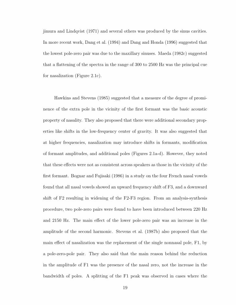
jimura and Lindqvist (1971) and several others was produced by the sinus cavities.

In more recent work, Dang et al. (1994) and Dang and Honda (1996) suggested that

the lowest pole-zero pair was due to the maxillary sinuses. Maeda (1982c) suggested

that a flattening of the spectra in the range of 300 to 2500 Hz was the principal cue

for nasalization (Figure 2.1c).

Hawkins and Stevens (1985) suggested that a measure of the degree of promi-

nence of the extra pole in the vicinity of the first formant was the basic acoustic

property of nasality. They also proposed that there were additional secondary prop-

erties like shifts in the low-frequency center of gravity. It was also suggested that

at higher frequencies, nasalization may introduce shifts in formants, modification

of formant amplitudes, and additional poles (Figures 2.1a-d). However, they noted

that these effects were not as consistent across speakers as those in the vicinity of the

first formant. Bognar and Fujisaki (1986) in a study on the four French nasal vowels

found that all nasal vowels showed an upward frequency shift of F3, and a downward

shift of F2 resulting in widening of the F2-F3 region. From an analysis-synthesis

procedure, two pole-zero pairs were found to have been introduced between 220 Hz

and 2150 Hz. The main effect of the lower pole-zero pair was an increase in the

amplitude of the second harmonic. Stevens et al. (1987b) also proposed that the

main effect of nasalization was the replacement of the single nonnasal pole, F1, by

a pole-zero-pole pair. They also said that the main reason behind the reduction

in the amplitude of F1 was the presence of the nasal zero, not the increase in the

bandwidth of poles. A splitting of the F1 peak was observed in cases where the

19

(a) Spectrogram of bomb (b) Spectrogram of been

(c) Comparison of spectral frames for /aa/ (d) Comparison of spectral frames for /iy/

Figure 2.1: Examples of the acoustic consequences of vowel nasalization to helpunderstand the acoustic correlates pointed out in the text. (a) Spectrogram of theword bomb. (b) Spectrogram of the word been. (c) Comparison of nasalized (dashedblack, extracted with a 30ms window around 0.365s) and non-nasalized (solid blue,extracted with a 30ms window around 0.165s) spectral frames for /aa/. It demon-strates the relative prominence of the low-frequency pole at 200 Hz, reduction inF1 amplitude, spectral flattening in 0-1300 Hz, movement in F3 and reduction inoverall amplitude. (d) Comparison of nasalized (dashed black, extracted with a30ms window around 0.245s) and non-nasalized (solid blue, extracted with a 30mswindow around 0.1s) spectral frames for /iy/. It demonstrates the appearance of anextra nasal pole near 1000 Hz, movement in F2 and reduction in overall amplitude.

20

nonnasal F1 frequency was close to the frequency of the nasal zero. Further, they

suggested that nasal poles at high frequencies occur with a very high density and

manifest themselves as small notches in the spectrum.

2.2 Perception of Vowel Nasalization

Several studies have shown the correspondence between the properties sug-

gested above and perception of nasalization. House and Stevens (1956) found that

the amplitude of F1 needed to be reduced by 8 dB for the nasality response to

reach the 50% level. Hattori et al. (1958) also performed a perceptual experiment

to confirm the correlation between the acoustic correlates suggested by them, and

the perception of nasalization. They concluded that adding the pole around 250 Hz

gave some perception of nasality, but adding the zero at 500 Hz did not. However,

the combination of the two gave a much improved perception of nasality. Further,

for high vowels like /iy/ and /uw/, it was necessary to modify the higher frequency

spectrum by adding additional poles between regular formants to produce the per-

cept of nasality. Maeda (1982c) confirmed the importance of spectral flattening at

low frequencies in producing the perception of nasality by listening tests.

Hawkins and Stevens (1985) used the Klatt synthesizer (Klatt, 1980) to simu-

late a continuum of CV syllables (/t/ followed by one of the five vowels /iy, ey, aa,

ow, uw/) from non-nasal to nasal. Nasalization was introduced by inserting a pole-

zero pair in the vicinity of the first formant. The degree of nasalization was varied

21

by changing the spacing between the pole and zero. Wider spacing of the pole-zero

pair was found to be necessary for the perception of nasality. Bognar and Fujisaki

(1986), in their perceptual study of nasalization of French vowels, evaluated the role

of the formant shifts and of pole-zero pairs on phonemic and phonetic judgements

of nasality of synthetic stimuli generated by using parameter values (i.e. F1, F2, F3

frequencies and the frequency separation between the extra pole-zero pair) which

varied between those for an oral /eh/ and its nasalized version /eh/. Their results

suggested that whatever one’s phonemic framework, a certain degree of pole-zero

separation is perceived as nasalization. However, they found that the phonemic sys-

tem of the French speaker strongly influenced his phonetic perception of an acoustic

feature like formant shift. In other words, the contribution of the formant shifts

and pole-zero separation was almost equal for the phonemic task of distinguishing

between /eh/ and /eh/, whereas the contribution of formant shifts was negligible

for the phonetic task of discriminating nasalized vowels from non-nasalized vowels

(that is, the listener only had to say whether the sound was nasalized or not, and

did not have to worry about specifying the exact phonemic identity of the sound).

Beddor (1993) presented an excellent review of past literature on the perception of

vowel nasalization.

Even though several researchers in the past have proposed a number of acousti-

cal and perceptual correlates of nasality, the following questions are still unanswered:

Is there a vowel and language independent acoustic correlate of nasality that listen-

ers use to differentiate nasalized vowels from oral vowels? Are these correlates also

22

independent of the reasons behind the introduction of nasalization (coarticulatory,

functional or phonemic)? Is the perception of nasalization affected by vowel prop-

erties like vowel height and vowel backness? And does nasalization lead to a change

in the vowel quality? These questions will now be discussed.

2.2.1 Independence from category of nasality

Although, there are no studies which directly address the question of similari-

ties/differences between the acoustic manifestations of the three different categories

of nasality, a lot of studies suggest that they are similar. Dickson (1962) performed

an acoustic study of nasality for the vowels /iy/ and /uw/ in the words ’beet’ and

’boot’ for 20 normal speakers, 20 speakers classified as having functional nasality,

and 20 speakers with cleft-palate and nasality. In this study, no means was found to

differentiate nasality in cleft-palate and non-cleft-palate individuals either in terms

of their acoustic spectra or the variability of the nasality judgements (listeners were

consistently able to judge nasality irrespective of what had caused it). Further, the

acoustic correlates found to occur in the spectrograms of the nasal speakers were

exactly the same as correlates that are usually cited for coarticulatory nasalization.

Other studies have cited similar acoustic correlates for languages with phonemic

nasalization (see Section 2.2.3).

23

2.2.2 Vowel Independence

All of the acoustic studies cited above (House and Stevens, 1956; Hattori et al.,

1958; Fant, 1960; Dickson, 1962; Fujimura and Lindqvist, 1971; Maeda, 1982b,c;

Hawkins and Stevens, 1985; Bognar and Fujisaki, 1986; Stevens et al., 1987b) have

shown that irrespective of the vowel identity, the most important and stable effects

of nasalization are in the low frequency regions. These effects are in the form of

prominence of the extra poles, modification of F1 amplitude and bandwidth, and

spectral flattening. Perceptual studies across different vowels have confirmed that

reduction in the amplitude of F1 (House and Stevens, 1956), spectral flattening

(Maeda, 1982c), or increasing separation between the extra pole-zero pair inserted

at low frequencies (Hawkins and Stevens, 1985) are sufficient to produce the percep-

tion of nasality. It seems, then, that there is a vowel independent cue for nasality.

Hawkins and Stevens (1985) went one step further and suggested that this vowel

independent property was a measure of the degree of spectral prominence in the F1

region.

Does vowel independence, however, mean that listeners use the same threshold

across all vowels to classify stimuli into oral and nasal? Or, is it that the acoustic

correlates used are the same but thresholds used are different for every vowel? It is

unclear at the moment what really happens, although results shown by Hawkins and

Stevens (1985) do show a small variation in thresholds across vowels. Further, does

this vowel independence also mean that listeners would be able to identify nasal-

24

ization in a vowel which does not exist in their native language? Or does listeners’

linguistic experience with a vowel train them in some basic acoustic characteristics

which enable them to identify nasalization in those vowels? Bognar and Fujisaki

(1986) have shown that a native speaker of Japanese, when asked to judge the pho-

netic quality (nasalized vs non-nasalized) of synthetic stimuli of a vowel which does

not belong to the phonetic system of his mother tongue, was able to correctly per-

ceive nasalization in the stimuli with increasing separation between the nasal pole

and zero. However, more experiments are required to confirm this for natural speech

stimuli.

2.2.3 Language Independence

Perceptual experiments using speakers of different languages with and with-

out phonemic nasalization have shown that different language groups give similar

responses for the presence or absence of nasalization. In a cross-language study

to investigate the effect of linguistic experience on the perception of oral-nasal dis-

tinction in vowels, Beddor and Strange (1982) presented articulatory synthesized

continua of [baa-baa] to Hindi and American English speaking subjects (nasaliza-

tion being phonemic for Hindi). They found no consistent differences across continua

in the identification responses of Hindi and American English speakers. In another

cross-language study on speakers of American English, Gujarati, Hindi and Bengali

(Gujarati, Hindi and Bengali have phonemic nasalization), Hawkins and Stevens

(1985) found no significant differences in the 50% crossover points of the identifica-

25

tion functions. They suggested the existence of a vowel and language independent

acoustic property of nasality and proposed that this measure was a measure of the

degree of spectral prominence in the vicinity of the first formant. They also pos-

tulated that there are one or more additional acoustic properties that may be used

to various degrees in different languages to enhance the contrast between a nasal

vowel and its non-nasal congener. Shifts in the center of gravity of the low-frequency

prominence and changes in overall spectral balance were cited as examples of such

additional secondary properties. In another cross-language study of the perception

of vowel nasalization in VC contexts using native speakers of Portugese, English and

French, which differ with respect to the occurence of nasal vowels in their phonologi-

cal systems, Stevens et al. (1987a) found that different language groups gave similar

responses with regard to the presence or absence of nasalization.

Even though it seems that speakers of different languages use the same acoustic

cues to make oral-nasal distinction among vowels, behavioral differences have been

found. Beddor and Strange (1982) found that the perception of oral-nasal vowel

distinction was categorical for Hindi speakers, and more continuous for speakers of

American English. Stevens et al. (1987a) found that the judgements of natural-

ness of the stimuli depended on the temporal characteristics of nasalization in the

stimuli. English listeners preferred some murmur along with brief nasalization in

the vowel, whereas French listeners preferred a longer duration of nasalization in

the vowel and gave little importance to the presence of a murmur. Responses of

Portugese listeners were intermediate.

26

Once again, the question arises whether the thresholds used to classify vowels

into oral and nasal are the same or different across languages? That is, will a system

for this purpose need to be trained again for every new language? It is unclear at

the moment, although results presented by Beddor and Strange (1982) and Hawkins

and Stevens (1985) suggest that the thresholds might be the same. However, it has

also been shown that even though the 50% crossover points might be similar, the

identification functions do get tuned for categorical perception when the speakers

native language has phonemic nasalization. Thus, speakers of these languages find

it harder to correctly perceive the degree of nasalization.

2.2.4 Effects of Vowel Properties on Perceived Nasalization

Studies using natural stimuli have shown that low vowels are perceived as

nasal more often than non-low vowels (Ali et al., 1971; Lintz and Sherman, 1961).

Studies using synthetic stimuli, however, have shown that low vowels need more

velar coupling to be perceived as nasal as compared to non-low vowels (Abramson

et al., 1981; House and Stevens, 1956; Maeda, 1982c). One plausible explanation

is as follows: high vowels are more closed in the oral cavity than low vowels, and

hence offer a higher resistance path (looking into the oral cavity from the coupling

point). Therefore, even a small coupling with the nasal cavity is sufficient to lower

the impedance enough to let a sufficient amount of air to pass through the nasal

cavity, thus making it nasalized. In the case of low vowels, however, the velum needs

27

to drop a lot more to reduce the impedance to a value equal to or lower than the

impedance offered by the oral cavity. Further, the apparent contradiction between

the results of studies using natural and synthetic stimuli can be explained by the fact

that low vowels are produced with a lower velum even in oral contexts (Ohala, 1971).

In a study with synthetic stimuli, Delattre and Monnot (1968) presented stim-

uli differing only in vowel duration to French and American English listeners and

found that shorter vowels were identified as oral and longer vowels as nasal. In this

study, vowel nasalization was held constant and was intermediate between that of

an oral and that of a nasal vowel in terms of the F1 amplitude. In another study,

Whalen and Beddor (1989) synthesized vowels /aa/, /iy/ and /uw/ with five vowel

durations and varying degree of velopharyngeal opening, and found that American

English listeners judged vowels with greater velopharyngeal opening, and the vowels

with longer duration as more nasal.

Perceived vowel nasality is also influenced by the phonetic context in which

the vowels occur. Lintz and Sherman (1961) showed that the perceived nasality was

less severe for syllables with a plosive environment than for syllables with a fricative

environment. Kawasaki (1986) found that perceived vowel nasality was enhanced

as adjacent nasal consonants were attenuated. Krakow and Beddor (1991) found

that nasal vowels presented in isolation or in oral context were more often correctly

judged as nasal, than when present in the original nasal context. These studies

show that listener’ knowledge of coarticulatory overlap leads them to attribute vowel

28

nasalization to the adjacent nasal contexts, thereby hearing nasal vowels in nasal

context as nonnasal. Further, in a study with listeners of a language with phonemic

nasalization, Lahiri and Marslen-Wilson (1991) found that vowel nasality was not

interpreted as a cue to the presence of a nasal consonant by such listeners.

2.2.5 Effects of Nasalization on perceived Vowel Properties

It has been suggested by Beddor and Hawkins (1990) that the height of vowels

is influenced by the location of the low-frequency center of gravity instead of just F1.

Introduction of extra poles in the low frequency region in nasalized vowels (either

above or below F1) leads to a change in the center of gravity of these vowels. Thus,

high and mid nasal vowels tend to sound like vowels of lower height, and low vowels

become higher. This was confirmed by Wright (1986) in a study of oral and nasal

counterparts of American English vowels /iy, ey, eh, ae, aa, ow, uh, uw/. This shift

was also confirmed by Arai (2004) in more recent experiments. Further, it has been

shown by Krakow et al. (1988) that, in the case of contextual nasalization, Ameri-

can English listeners adjust for the low frequency spectral effects of nasalization to

correctly perceive vowel height. However, in the case of noncontextual nasalization,

the perceptual effect of this spectral shift was to lower the perceived vowel height.

Arai (2004) has also shown that a nasalized vowel is recognized with higher accuracy

than a nonnasal vowel with the same formant frequencies as the nasal vowel, thus,

confirming the existence of a compensation effect. Arai (2005) has also tried to

study the compensation effect for formant shifts on the production side. In a study

29

with American English vowels /iy, ih, eh, ah, ae, aa/ he found that the positions of

the articulators showed no compensation effect except for vowel /aa/. It was con-

cluded that there might be no compensation effect on the production side because

American English does not distinguish between oral and nasal vowels phonemically.

It could, however, be true for languages with phonemic nasalization. No such con-

sistent effects of nasalization have been found on perceived vowel backness until now.

In effect, then, the low frequency spectral effects of nasalization lead to a con-

traction of the perceptual space of nasalized vowels. Bond (1975) confirmed this

by showing that vowels excised from nasal contexts are more often misidentified

than are vowels from oral contexts. Mohr and Wang (1968) and Wright (1986) also

showed that the perceptual distance between members of nasal vowel pairs was con-

sistently less than that between oral vowels.

2.3 Acoustic Parameters

This section describes the Acoustic Parameters (APs) that have been suggested

by various researchers in the past to capture the acoustic correlates described earlier

in this chapter. The algorithms suggested may or may not be automatic.

Glass (1984) and Glass and Zue (1985) developed a set of APs which were

automatically extracted and tested on a database of 200 words, each spoken by 3

30

male and 3 female speakers. To capture nasality they used the following parameters:

(1) the center of mass in 0-1000 Hz, (2) the standard deviation around the center

of mass, (3) the maximum and minimum percentage of time there is an extra pole

in the low frequency region, (4) the maximum value of the average dip between the

first pole and the extra pole, and (5) the minimum value of the average difference

between the first pole and the extra pole. Parameters 1 and 2 tried to capture the

smearing in the first formant region. Parameter 3 tried to capture the presence of

the extra nasal pole in the first formant region, and Parameters 4 and 5 tried to

capture the distinctiveness of the extra nasal pole due to a higher amplitude and a

deeper valley. They were able to obtain an overall accuracy of 74% correct nonnasal-

nasal distinction using a circular evaluation procedure.

Huffman (1990) identified the average difference between the amplitude of the

first formant (A1) and the first harmonic (H1), and change in A1−H1 over time as

good parameters to capture the decrease in A1 with the introduction of nasality. In

this study, listeners were presented with oral and coarticulatorily nasalized vowels,

and the results were correlated with the proposed APs. The nasalized vowels con-

fused as oral vowels were those with higher overall values of A1−H1. However, the

oral vowels which were sometimes confused to be nasal vowels were the ones which

showed a marked decrease in A1 − H1 over the course of the vowel rather than a

lower value of A1−H1. These results highlighted the role of dynamic information

in the perception of nasality.

31

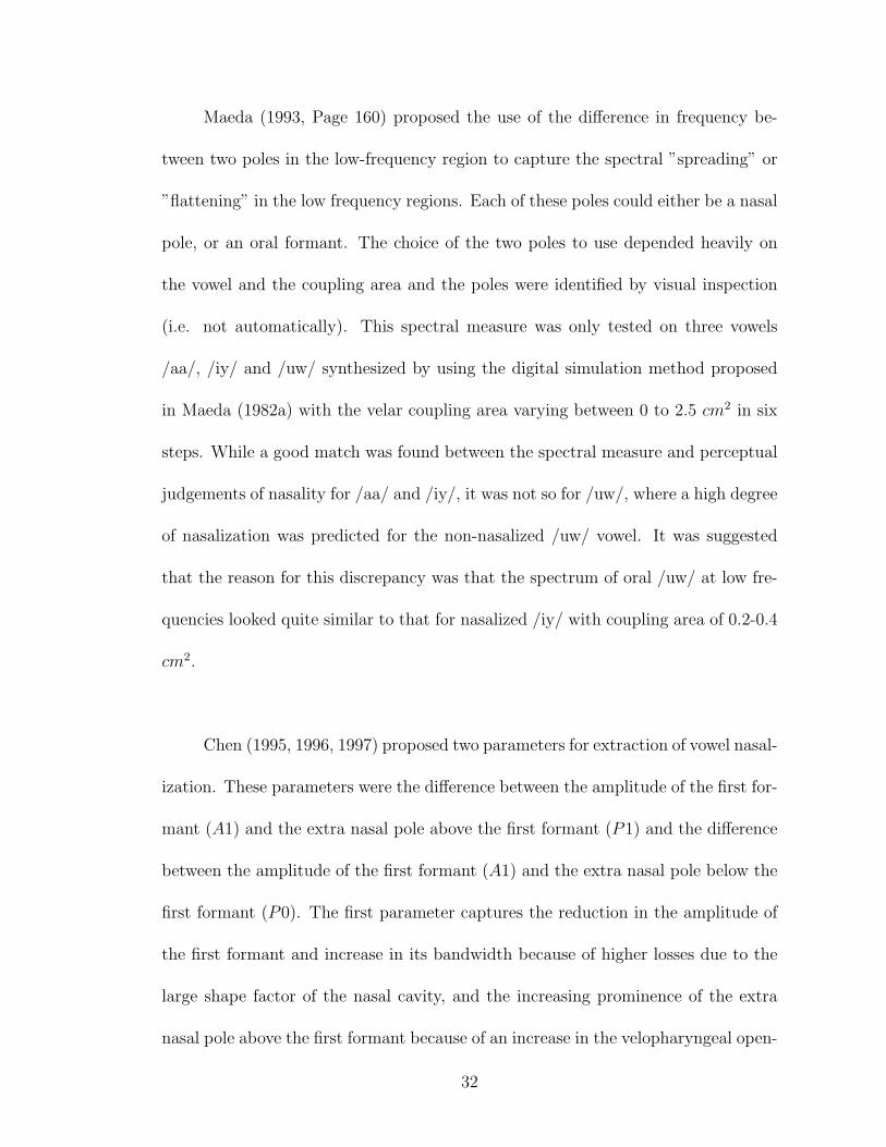
Maeda (1993, Page 160) proposed the use of the difference in frequency be-

tween two poles in the low-frequency region to capture the spectral ”spreading” or

”flattening” in the low frequency regions. Each of these poles could either be a nasal

pole, or an oral formant. The choice of the two poles to use depended heavily on

the vowel and the coupling area and the poles were identified by visual inspection

(i.e. not automatically). This spectral measure was only tested on three vowels

/aa/, /iy/ and /uw/ synthesized by using the digital simulation method proposed

in Maeda (1982a) with the velar coupling area varying between 0 to 2.5 cm2 in six

steps. While a good match was found between the spectral measure and perceptual

judgements of nasality for /aa/ and /iy/, it was not so for /uw/, where a high degree

of nasalization was predicted for the non-nasalized /uw/ vowel. It was suggested

that the reason for this discrepancy was that the spectrum of oral /uw/ at low fre-

quencies looked quite similar to that for nasalized /iy/ with coupling area of 0.2-0.4

cm2.

Chen (1995, 1996, 1997) proposed two parameters for extraction of vowel nasal-

ization. These parameters were the difference between the amplitude of the first for-

mant (A1) and the extra nasal pole above the first formant (P1) and the difference

between the amplitude of the first formant (A1) and the extra nasal pole below the

first formant (P0). The first parameter captures the reduction in the amplitude of

the first formant and increase in its bandwidth because of higher losses due to the

large shape factor of the nasal cavity, and the increasing prominence of the extra

nasal pole above the first formant because of an increase in the velopharyngeal open-

32

ing. The second parameter captures the nasal prominence at very low frequencies

introduced because of coupling to the paranasal sinuses. P1 was estimated by using

the amplitude of the highest peak harmonic around 950 Hz, and P0 was chosen

as the amplitude of the harmonic with the greatest amplitude at low frequencies.

Chen (1995, 1997) also modified these parameters to make them independent of

the vowel context. However, these parameters were not automatically extracted

from the speech signal. In later work, Chen (2000a,b) also used these parameters

in detecting the presence of nasal consonants for cases where the nasal murmur was

missing.

Cairns et al. (1994, 1996b,a) proposed the use of a nonlinear operator to de-

tect hypernasality in speech in a noninvasive manner. The basic idea behind the

approach was that normal speech is composed of just oral formants, whereas nasal-

ized speech is composed of oral formants, nasal poles and zeros. Therefore, lowpass

filtering with a properly selected cutoff frequency would filter just the first formant

for normal speech, and a combination of first oral formant, nasal poles and zeros

for hypernasal speech. However, bandpass filtering around the first formant would

only return first formant in both cases. This multicomponent nature of hypernasal

speech was exploited using a nonlinear operator called the Teager Energy opera-

tor. They used the correlation coefficient between the Teager energy profiles of

lowpass filtered and bandpass filtered speech as a measure of hypernasality, where

a low value of the correlation coefficient suggested hypernasality. The final deci-

sion making was done with a likelihood ratio detector. Even though the correlation

33

parameter was extracted automatically, this approach had several problems: First,

back vowels were not studied because of the difficulty in filtering out the second

formant. This raises a question about its application across all vowels. Second, the

parameters of the probability densities used for the likelihood ratio detector varied

over different speaker groups and over different vowels. Finally, there were different

thresholds for different vowels and different speaker groups. These limitations make

it too restrictive for a generalized application across all speakers and vowels.

Hasegawa-Johnson et al. (2004, 2005) also worked on vowel nasalization de-

tectors using a large set of APs which included Mel-Frequency Cepstral Coefficients

(MFCCs), Knowledge-based APs (Bitar, 1997a), rate-scale parameters (Mesgarani

et al., 2004) and formant parameters (Zheng and Hasegawa-Johnson, 2004). All

the acoustic observations were generated automatically once every 5 ms. MFCCs

generated once every 10ms were also included. A frame-based vowel-independent

common classifier to distinguish nasal frames from non-nasal frames using these pa-

rameters in a linear SVM framework was able to achieve 62.96% accuracy on a test

set extracted from a combination of WS96 and WS97 databases.

Vijayalakshmi and Reddy (2005a) used the modified group delay function pro-

posed by Murthy and Gadde (2003) and Hegde et al. (2004, 2005) to extract APs

for detecting hypernasality. The idea behind using the modified group delay func-

tion was that conventional formant extraction techniques like Linear Prediction and

Cepstral smoothing are unable to resolve the extra pole around 250 Hz introduced

34

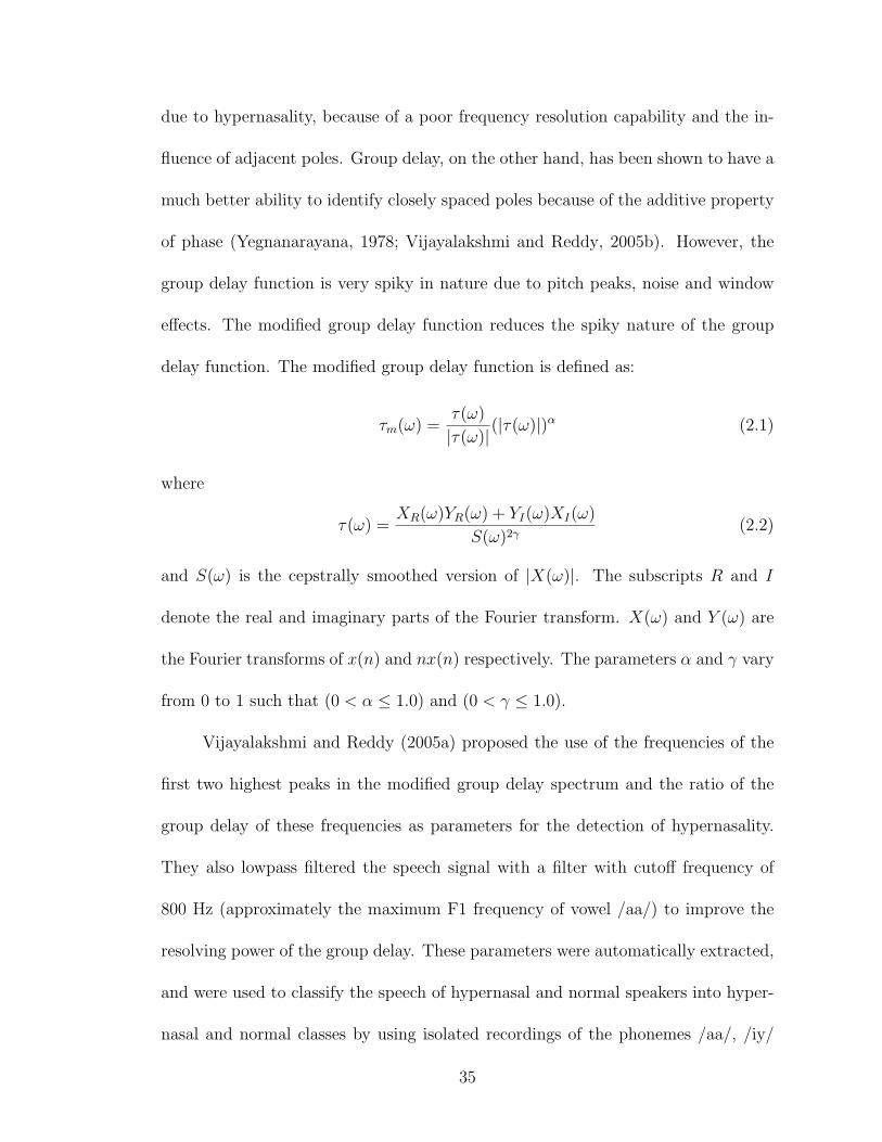
due to hypernasality, because of a poor frequency resolution capability and the in-

fluence of adjacent poles. Group delay, on the other hand, has been shown to have a

much better ability to identify closely spaced poles because of the additive property

of phase (Yegnanarayana, 1978; Vijayalakshmi and Reddy, 2005b). However, the

group delay function is very spiky in nature due to pitch peaks, noise and window

effects. The modified group delay function reduces the spiky nature of the group

delay function. The modified group delay function is defined as:

τm(ω) =τ(ω)

|τ(ω)|(|τ(ω)|)α (2.1)

where

τ(ω) =XR(ω)YR(ω) + YI(ω)XI(ω)

S(ω)2γ(2.2)

and S(ω) is the cepstrally smoothed version of |X(ω)|. The subscripts R and I

denote the real and imaginary parts of the Fourier transform. X(ω) and Y (ω) are

the Fourier transforms of x(n) and nx(n) respectively. The parameters α and γ vary

from 0 to 1 such that (0 < α ≤ 1.0) and (0 < γ ≤ 1.0).

Vijayalakshmi and Reddy (2005a) proposed the use of the frequencies of the

first two highest peaks in the modified group delay spectrum and the ratio of the

group delay of these frequencies as parameters for the detection of hypernasality.

They also lowpass filtered the speech signal with a filter with cutoff frequency of

800 Hz (approximately the maximum F1 frequency of vowel /aa/) to improve the

resolving power of the group delay. These parameters were automatically extracted,

and were used to classify the speech of hypernasal and normal speakers into hyper-

nasal and normal classes by using isolated recordings of the phonemes /aa/, /iy/

35

and /uw/ for both training and testing. The classifier was found to be able to give

a correct hypernasal/normal decision in almost 85% of the cases.

2.4 Chapter Summary

The following acoustic correlates for vowel nasalization have been reported by

one or more researchers in past literature:

1. Reduction in first formant amplitude.

2. Increase in first formant bandwidth.

3. Increase in first formant frequency.

4. Extra pole-zero pairs in the first formant region.

(a) Below the first formant (in the range of 200-500 Hz approx).

(b) Above the first formant (in the range of 700-2000 Hz approx). The exact

location of the pole and zero changes with change in the vowel and the

degree of coupling.

5. Shifts in the low-frequency center of gravity.

6. Spectral flattening in the range of 300-2500 Hz.

7. Changes in the amplitude of the second formant and shift in its frequency.

8. Changes in the amplitude of the third formant and shift in its frequency.

36

9. Extra pole-zero pair in the third formant region.

10. Reduction in overall amplitude of the vowel.

The perceptual importance of most of these parameters has been established

by perceptual experiments. It has also been said by some researchers that the

higher frequency effects are not very stable across speakers. Thus, the most impor-

tant and stable effects of vowel nasalization are in the low-frequency region. The

exact acoustic consequences of nasalization have been shown to vary with changes

in vowel identity, speaker and the degree of coupling. The survey of the litera-

ture suggests the presence of vowel and language independent acoustic correlates of

nasalization. However, it remains to be seen whether this variation also means that

the same vowel nasalization detector will work across vowels and languages without

re-training of the thresholds. Perception of nasalization is not only affected by vowel

properties, but nasalization itself also affects the perception of vowel properties.

Several attempts have been made at capturing one or more of the acoustic

correlates listed above using APs based on automatic/semi-automatic/manual al-

gorithms. However, fully automatic algorithms to extract APs which capture the

acoustic correlates of nasalization reliably irrespective of the vowel identity and

speaker still remain elusive. This study will attempt to propose knowledge-based

APs for vowel nasalization based on fully automatic algorithms.

37

Despite the extensive literature on vowel nasalization, it is still not clear why

nasalization introduces such dynamic and varied acoustic consequences. The anal-

ysis presented in Chapter 4 attempts to explain the reasons behind the complex

acoustic effects of nasalization and the variation because of changes in vowels and

speakers. This analysis should be very helpful in specifying knowledge-based APs

for the automatic detection of vowel nasalization.

38

Chapter 3

Databases, Tools and Methodology

This chapter documents the groundwork that has been done for the develop-

ment of Acoustic Parameters (APs) for automatic detection of vowel nasalization.

This includes details of the databases that were used in this study, and the tools

that were developed or used to understand the spectra of nasalized vowels along

with a detailed description of the task at hand, the classifier used, the training set

selection methodology and the training and classification procedure.

3.1 Databases

This section describes the databases that will be used in the experiments in

this thesis. StoryDB is a database of isolated words. This database was used

both for comparing the simulated transfer functions with real spectra in the vocal

tract modeling study presented in Chapter 4, and for testing the proposed APs in

Chapter 6. The simplified conditions in this database made it ideal for use as a

control database to tune the proposed APs, and test them for a simple case. The

other databases were only used to test the performance of the proposed APs. These

databases are continuous speech databases and present increasingly complicated

conditions with a large number of speakers and significant contextual influences.

TIMIT (1990) was recorded at a sampling rate of 16 KHz and consists of read

39

speech. WS96, WS97 (Godfrey et al., 1992) and OGI Multilanguage (Muthusamy

et al., 1992) are telephone speech databases recorded at a sampling rate of 8 KHz

and contain spontaneous speech.

3.1.1 StoryDB

Acoustic recordings of seven vowels /aa, ae, ah, eh, ih, iy, uw/ in nasalized

and non-nasalized contexts were obtained for the same speaker for whom the vocal

tract and nasal tract area functions used in Chapter 4 were available. A list of the

recorded words is given in Table 3.1. The database was recorded with an AKG

CK92 condenser microphone and was coupled to an AKG SE 300 B Preamp. The

signal was recorded directly to disk via a Kay Elemetrics 4400. The words were

carefully articulated in isolation and recorded under normal nasal condition, and

after the application of Afrin to clear the nasal cavity. The data was recorded both

in upright standing position, and in supine position to simulate the conditions during

MRI recordings. The data was originally recorded at a sampling rate of 44100 Hz,

and was downsampled to 16000 Hz. Four instances of each word were recorded to

give a total of 56 (words) x 4 (conditions: standing and supine, with and without

the application of Afrin) x 4 (instances) = 896 words. The database was divided

equally into train and test databases by keeping two instances of each word in the

training database, and two in the testing database. All the words were manually

segmented to mark the beginning and ending of the vowels in consideration.

For the purposes of testing the proposed APs, it was assumed that every vowel

40

Table 3.1: List of recorded words.

Vowel Words without nasals Words with nasals

/iy/ bee, seas been, queen, deem, seem, scenes, machines

/uw/ woo, boo wound, womb, boon, moon, doom, groom

/aa/ pop, bob font, conned, pomp, bomb, con, tom

/ae/ cat, cap cant, banned, camp, lamb, ban, dam

/ah/ hut, dub hunt, gunned, bump, dumb, bun, done

/eh/ bet, get bent, penned, temp, member, ben, gem

/ih/ hit, pip hint, pinned, pimp, limb, bin, dim

before a nasal consonant is nasalized. This assumption is especially valid in this

case because most of the words were single syllable words, and the nasal consonant

was always introduced in the syllable-final position to maximize the possibility of

nasalization during the vowel region. Further, in a lot of the words, the nasal was

immediately followed by a stop. This has been previously reported to lead to a

missing murmur condition (Chen, 2000b), thus leaving nasalization in the preceding

vowel as the only cue for the presence of the nasal consonant, and hopefully giving

a stronger degree of nasalization.

3.1.2 TIMIT

TIMIT (1990) contains a total of 6300 sentences, 10 sentences spoken by each

of 630 speakers (438 males, 192 females) from 8 major dialect regions of the United

41

States. The speech data was recorded digitally at a sampling rate of 20 KHz in a

relatively quiet environment with a peak signal to noise ratio of 29 dB. The data

was recorded simultaneously on a pressure-sensitive microphone and a Sennheiser

close-talking microphone. After recording the database was downsampled to 16 KHz

(Zue et al., 1990). The database was divided into training and testing sets.

Although the speech data was phonetically transcribed, the nasalization dia-

critic was not marked in this database. Therefore, while using this database, it was

assumed that all vowels preceding nasal consonants are nasalized. The set of nasal

consonants included /m/, /n/, /ng/ and /nx/. Further, all syllabic nasals (/em/,

/en/ and /eng/) were considered to be nasalized vowels. Vowels were considered

to be oral/non-nasalized when they were not in the context of nasal consonants or

syllabic nasals. This definition would, however, classify vowels in words like /film/

as oral vowels even though the vowel (being in the same syllable as the nasal con-

sonant) would most likely be nasalized due to anticipatory coarticulation with the

syllable-final nasal consonant /m/. Since, such cases may be somewhat ambiguous,

they were removed from consideration by not considering vowels as oral when the

second phoneme after the vowel was a nasal consonant. This condition is similar

to that imposed by (Glass and Zue, 1985). In the case of vowels following nasal

consonants, nasalization might not be very strong. Hence, these cases were also

removed from consideration.

It is also important to note that a nasal will probably introduce nasalization in

the preceding vowel only when they belong to the same syllable. However, the above

assumption about all vowels preceding nasal consonants being nasalized was essential

42

because syllable boundaries were not marked in TIMIT. While this assumption

would classify all vowels preceding syllable-initial nasal consonants as nasalized,

they might not actually be nasalized. Hence, this can be a major source of potential

errors in all experiments with TIMIT.

3.1.3 WS96 and WS97

The WS96 database is a part of the switchboard corpus (Godfrey et al., 1992)

which was phonetically transcribed in a workshop at Johns Hopkins University in

1996. The database consists of telephone bandwidth spontaneous speech conversa-

tions recorded at a sampling rate of 8 KHz. Diacritics were used to denote significant

deviation from the typical pattern. A diacritic was used when the phonetic prop-

erty was a significant departure from canonical, and where it applied to at least

half of the segment duration (or in instances where less than half, the duration

was appreciable, as would be the case for a stressed or emphasized syllable). Thus,

the nasalization diacritic indicated nasalization of a usually non-nasalized segment.

Therefore, a vowel was marked as nasalized if the duration of nasalization during

the vowel region was appreciable, irrespective of the presence of a nasal consonant

adjacent to it (Note that vowels are non-nasalized segments in their canonical form).

The WS97 database is also a part of the switchboard corpus which was tran-

scribed in a workshop at Johns Hopkins University in 1997. In WS97, the initial

automatically generated phone alignments were post-processed to group the phone

43

labels into syllabic units (based on the rules from Kahn (1976)). Transcribers were

only asked to ensure the correct alignment of syllable units and specification of the

phonetic composition of these units. The phoneme boundaries in WS97 were then

generated by automatic procedures with the hope that correct syllable boundaries

should give sufficient knowledge to get correct phoneme boundaries by automatic

procedures. In WS96, on the other hand, transcribers were asked to correct both

the phone labels and the phone alignments generated by automatic procedures.

Therefore, the phoneme boundaries in WS97 may not be as accurate as WS96.

WS96 and WS97 databases were combined together (the combined dataset

would, henceforth, be referred to as WS96/97 database) and divided into training

and testing databases by alternately selecting files from the combined list leading to

a total of 2552 files in the training database, and 2547 files in the testing database.

Note that, the number of files in the training and testing databases used in this study

is not the same because some of the files had discontinuities which were distorting

the calculation of the parameters. Thus, these files (total of 13) were removed

from consideration. All syllabic nasals and vowels with a nasalization diacritic were

considered to be nasalized vowels for the purpose of testing the performance of APs.

Oral vowels were selected in the same manner as described for the TIMIT database

above.

44

3.1.4 OGI Multilanguage Telephone Speech Corpus

The OGI Multi-language Telephone Speech Corpus (Muthusamy et al., 1992)

consists of telephone speech from 11 languages: English, Farsi, French, German,

Hindi, Japanese, Korean, Mandarin, Spanish, Tamil and Vietnamese. The corpus

contains fixed vocabulary utterances, as well as fluent continuous speech. The data

was recorded at a sampling rate of 8 KHz and consisted of a total of 12152 speech

files spoken by 2052 speakers across all languages. Out of these files, 619 were

phonetically transcribed: English (208), German (101), Hindi (68), Japanese (64),

Mandarin (70) and Spanish (108). Out of these six languages only Hindi has distinc-

tive phonemic nasalization. The nasalization diacritic was used in the fine phonetic

transcription to mark phonemic nasalization (that is, when the nasalization was

unpredictable). When nasalization was predictable by phonological rule (i.e., when

in the context of a neighboring nasal) it was not labeled. However, the protocol

also specified that since nasal deletion is a common phenomenon in fast speech,

if acoustic or auditory evidence signaling nasality remained, but no distinct nasal

was evident in the signal, the nasal diacritic should still be used so that the phone-

mic level transcription can be reproduced without lexical knowledge. An informal

inspection of all the vowels marked as phonemically nasalized and the words con-

taining those vowels suggested that most of the vowels were actually phonemically

nasalized.

For the purpose of evaluation of the performance of the APs, all vowels before

nasal consonants were considered to be coarticulatorily nasalized, and all vowels with

45

a nasalization diacritic were considered to be phonemically nasalized. No syllabic

nasals were marked in the database. Oral vowels were selected in the same manner

as described for the TIMIT database above. Note that Hindi has a larger set of nasal

consonants as compared to English. Further, this database also has some English

words although most of the vowels marked as being phonemically nasalized are from

Hindi.

3.2 Tools

3.2.1 Vocal tract modeling

All simulations shown in Chapter 4 have been performed using a computerized

model of the vocal tract called VTAR (Zhang and Espy-Wilson, 2004) which has

been developed in our lab. This model was initially developed for the simulation

of oral vowels and lateral sounds. In this work, the model was extended so that it

could simulate the spectra of nasalized vowels with multiple sidebranches. Further,

additional code was added so that the model could also generate the impedance

at every point in the vocal tract and nasal tract along with pressure and volume

velocity. A brief description of the procedure used to calculate the transfer functions

and the susceptance plots from vocal tract and nasal tract area functions is as

follows:

The input and output pressures (pin and pout) and volume velocities (Uin and

46

Uout) of a section of the vocal tract are related by the transfer matrix pin

Uin

=

A B

C D

pout

Uout

(3.1)

where A, B, C, and D depend on the properties of the air and the vocal tract walls

and can be calculated by using the transmission-line model (as shown in Zhang and

Espy-Wilson (2004)). The transfer function can then be calculated as

Uout

Uin

=1

CZout + D(3.2)

where Zout = pout/Uout. The impedance at a point in the vocal tract can be obtained

as a byproduct of the transfer function calculation. Hence,

Zin =pin

Uin

=AZout + B

CZout + D(3.3)

Every branch constitutes a parallel path. Therefore, Zout1 = 1/(1/Zin2 +

1/Zin3) (see Figure 3.1). Further, a branch coupling matrix can be used to relate

the state variables across the branching point. Therefore, for Figure 3.1 pout1

Uout1

=

1 0

1/Zin3 1

pin2

Uin2

(3.4)

and pout1

Uout1

=

1 0

1/Zin2 1

pin3

Uin3

(3.5)

where Zin2 and Zin3 are obtained as shown in equation 3.3. Thus, the impedance

and transfer function at any point in the vocal tract can be found by starting at

the output and successively considering each section of the vocal tract without any

47

Figure 3.1: An illustration to show the procedure to calculate the transfer functionsand susceptance plots.

branches, finding Zin, Uin and pin for that section, adding the parallel contribution of

any branches, and proceeding in that manner to obtain the required input impedance

and the transfer function from the input to that particular output. This procedure

can, therefore, be used to obtain Zin1, Zin2, Zin3, Uout2/Uin1 and Uout3/Uin1. The

susceptance B is equal to the imaginary part of the inverse of impedance Z (i.e. the

admittance). Thus, plotting the values of impedance/susceptance and the transfer

function with respect to frequency generates the impedance/susceptance and the

transfer function plots.

To generate good impedance/susceptance plots, losses in the model need to be

removed. Losses in the model can be removed by removing the resistive elements

from the circuit. This can be achieved by assuming zero resistance due to flow

viscosity, zero heat conduction and infinite wall resistance to remove the loss due to

wall vibrations. It should also be noted that for this lossless case,

Bin =1

Zin

=Uin

pin

=CZout + D

AZout + B(3.6)

where the susceptance, Bin = ∞ if either CZout + D = ∞ or AZout + B = 0. Thus,

48

equations 3.2 and 3.6 also show that the transfer function does not necessarily

have zeros when Bin = ∞. The transfer function will, however, have zeros when

CZout + D = ∞.

3.3 Methodology

3.3.1 Task

Given a vowel segment declare whether it is nasalized, or not.

3.3.2 Classifier Used

The main theme of this study is to propose knowledge-based APs for the

automatic detection of vowel nasalization. Hence, the choice of classifier is irrelevant,

as long as the same experimental conditions are used to compare the results obtained

with APs proposed in this study and the APs proposed by other researchers. Support

Vector Machines (SVMs) (Burges, 1998; Vapnik, 1995) were used as the classifier

of choice in this study, primarily for reasons of compatibility with the rest of the

back-end proposed in Juneja (2004). Secondary reasons include the inherent merits

of SVMs as classifiers as opposed to other methods. SVMs have a relatively good

generalization capability with less amount of training data, and they have been

particularly well developed for binary classification tasks. Further, they are scalable

for high dimensional data without a corresponding increase in the number of training

samples. The experiments were carried out using the SVMlight toolkit (Joachims,

1999).

49

3.3.3 Training Set Selection

The training data was collected by considering every oral and nasalized vowel

in succession (ground truth decided by the procedure described above), and selecting

only the middle 1/3rd of the frames for oral vowels and the last 1/3rd of the frames

for nasalized vowels. Although all the vowels which are considered as nasalized have

a nasal consonant adjacent to them, the coarticulatory effect of the nasal consonant

may not spread all through the vowel. Thus, using only the last 1/3rd of the frames

maximizes the possibility of these frames being truly nasalized. Further, for oral

vowels the middle 1/3rd of the frames should have the least contextual influence.

Therefore, this 1/3rd selection rule minimizes the possibility of the inclusion of

ambiguous oral or nasalized vowel frames in the training data.

Once the pool of data had been collected for the oral and nasalized vowel

classes, a set number of frames were randomly selected from this set to ensure that

frames from all different vowels were included in the training set. The random

selection of a set number of frames also ensured that the same number of frames

were selected from both the oral and nasalized vowel classes. It must be noted, that

frames extracted from Syllabic nasals were not included in the training set, but they

were tested in the performance evaluation.

3.3.4 SVM Training Procedure

The training of the SVM classifiers was done in two passes. In the first pass,

the SVM classifier using a linear kernel was trained multiple number of times by

50

randomly selecting a variable number of training samples from the complete pool

of data, and the training set size used in the classifier which gave the least error on

a validation set was selected for future training. In the second pass, this selected

training set size was used to randomly select the samples from the pool of data,

and to train SVM classifiers with both Linear and Radial Basis Function (RBF)

kernels. The above procedure was not followed separately for classifiers with RBF

kernels because the training of SVMs with RBF kernels can be computationally very

expensive.

3.3.5 SVM Classification Procedure

Once the SVM outputs were obtained for the training samples, the outputs

were mapped to pseudo-posteriors using a histogram. If N(g, d = +1) is the number

of training examples belonging to the positive class for which the SVM discriminant

had a value of g, the histogram posterior estimate is given by:

P (d = +1/g) =N(g, d = +1)

N(g, d = +1) + N(g, d = −1)(3.7)

Histogram counts were always be obtained by using the same number of sam-

ples for the positive and negative classes, so that the pseudo-posterior P (d/g) is

proportional to the true likelihood P (g/d). Given that the pseudo-posteriors are

proportional to the true likelihoods, and assuming frame independence, the proba-

bility for a segment to belong to the positive class can be obtained by multiplying

the pseudo-posteriors for each frame in the segment. Thus a vowel segment was

51

declared as nasalized if:

i=framen∏i=frame1

Pnasal(i) >i=framen∏i=frame1

Poral(i) (3.8)

where, Pnasal(i) = Probability that the ith frame is nasalized.

Poral(i) = 1− Pnasal(i) = Probability that the ith frame is non-nasalized.

3.3.6 Chance Normalization

If, in any case, the number of samples belonging to the positive and negative

classes is different, the accuracy was normalized so that the chance performance was

50%. This was achieved as follows:

A = 50× N11

N11 + N1,−1

+ 50× N−1,−1

N−1,1 + N−1,−1

(3.9)

where, Nij is the number of test tokens of category i classified as category j, and

i, j ∈ {−1, 1}.

3.4 Chapter Summary

In this chapter, a discussion of all the databases used in this thesis was pre-

sented along with a detailed description of the procedure used to calculate the

transfer functions and the susceptance plots which have been used extensively in

the next chapter to analyze vowel nasalization. A brief description of the training

and classification procedure used to evaluate the performance of the APs proposed

in Chapter 5 was also provided.

52

Chapter 4

Vocal Tract Modeling

Even after so many years of research, automatically extractable APs for vowel

nasalization, which work well independent of vowel context and language, have not

been found. Thus, further investigation is needed to better understand the spectral

effects of all the articulators involved in the production of nasalized vowels. This

includes understanding the effects of changes in velar coupling area on the nasalized

vowel spectra, the effects of asymmetry of the two nasal passages, and the effects of

paranasal cavities (also called sinuses).

Magnetic Resonance Imaging (MRI) has become a standard for volumetric

imaging of the vocal tract during sustained production of speech sounds (Alwan

et al., 1997; Baer et al., 1991; Moore, 1992; Narayanan et al., 1995, 1997). Dang et al.

(1994) used MRI to make detailed measurements of the nasal and paranasal cavities

and explore the acoustical effects of the asymmetry between the two nasal passages,

and the effects of the paranasal cavities on the spectra of nasal consonants. Story

et al. (1996) used MRI to create an inventory of speaker-specific, three-dimensional,

vocal tract air space shapes for 12 vowels, 3 nasals and 3 plosives. They also imaged

the nasal tract of the same speaker along with his left and right maxillary sinuses

and sphenoidal sinuses (Story, 1995).

Hardly any attempts have ever been made to analyze nasalized vowels using

53

real anatomical data recorded through MRI. This chapter, therefore, focuses on un-

derstanding the salient features of nasalization and the sources of acoustic variability

in nasalized vowels through vocal tract modeling simulations based on area func-

tions of the vocal tract and nasal tract of one American English speaker recorded

by Story (1995) and Story et al. (1996) using MRI. The analysis presented in this

chapter focuses on the vowels /iy/ and /aa/. However, area functions for the vow-

els /ae/, /uw/, /ah/, /eh/ and /ih/ were also available. Therefore, corresponding

simulations for these vowels have been reproduced in Appendix B.

4.1 Area Functions based on MRI

The areas of the vocal tract (oral cavity and pharyngeal cavity) for the vowels

/iy/ and /aa/, the nasal cavity, the Maxillary Sinuses (MS), and the Sphenoidal

Sinus (SS) for one American English speaker were obtained from MRI recordings

obtained by Story (1995) and Story et al. (1996). This data is reproduced in Fig-

ure 4.1. Note that, only two of the sinuses (SS and MS) were accounted for here,

since the area functions were only recorded for these sinuses. According to one of

the authors of Story et al. (1996), no connection to the main nasal passages could

be reliably measured for Ethmoidal Sinuses (ES) and Frontal Sinuses (FS), hence

they were not included. Further, for SS there were two ostia, but no visible di-

vision into two chambers was observed for the sinus. As a result, the ostial areas

were summed and the cross-sectional area of the sinus was measured as one chamber.

54

Figure 4.1: Areas for the oral cavity, nasal cavity, maxillary sinuses and sphenoidalsinus.

It is important to note that data for the nasal cavity was recorded during

normal breathing. This was done both with and without the application of Afrin (a

nasal decongestant) which shrinks the mucous membrane in the nasal cavity. The

area functions show considerable asymmetry between the left and right passages of

the nasal tract. The right passage was completely blocked for this subject without

the application of Afrin. This thesis will only use the data after the application

of Afrin, because although the structure of the nasal cavity is constant, the exact

area functions and the loss characteristics of the nasal cavity can vary considerably

over time because of the condition of the mucous membrane. Application of Afrin

gives a much more consistent result over time. Further, the area functions recorded

after the application of Afrin are also the most repeatable for subsequent audio

recordings. Although the area functions during the production of nasalized vowels

55

(a) (b)

(c)

Figure 4.2: Structure of the vocal tract model used in this study. (a) Simplifiedstructure used in Section 4.3.1, (b) Simplified structure used in Section 4.3.2, (c)Complete structure. G = Glottis, L = Lips, N = Nostrils, NL = Left Nostril, NR

= Right Nostril, RMS = Right Maxillary Sinus, LMS = Left Maxillary Sinus, SS= Sphenoidal Sinus, Bp = susceptance of the pharyngeal cavity, Bo = susceptanceof the oral cavity, Bn = susceptance of the nasal cavity, Bl = susceptance of theleft nasal passage, and Br = susceptance of the right nasal passage. The black dotmarks the coupling location.

were not available, the area functions for the stationary nasal tract were combined

with the data for the oral tract with a variable coupling area to approximately model

the nasalized vowels.

4.2 Method

In this study, VTAR (Zhang and Espy-Wilson, 2004), a computer vocal tract

model, was used to simulate the spectra for nasalized vowels with successive addition

of complexity to the nasal cavity to highlight the effects of each addition. Given

56

(a) (b)

Figure 4.3: Procedure to get the area functions for the oral and nasal cavity withincrease in coupling area: (a) Flowchart, (b) An example to illustrate the changesin nasopharynx areas and areas of corresponding sections of the oral cavity whenthe coupling area is changed from 0.0 cm2 to 1.0 cm2.

the description of area functions in Section 4.1, the complete structure of the model

of the vocal tract and the nasal tract used in this study is shown schematically in

Figure 4.2c. Section 4.3.1 analyzes the acoustic changes due to the introduction of

coupling between the vocal tract and the nasal tract, and due to changes in the

coupling area. Hence, in this section a simplified model of the vocal tract and nasal

tract (shown schematically in Figure 4.2a) is considered. Section 4.3.2 analyzes

the effects of asymmetry between the left and right nasal passages, and therefore,

the model shown in Figure 4.2b adds the complexity due to nasal bifurcation in

the model considered in this section. Section 4.3.3 examines the effects of MS and

SS on the acoustic spectrum. Hence, the model shown in Figure 4.2c is used for

simulations in this section.

The nasal cavity data shown in Figure 4.1 were combined with the oral cavity

57

data for the vowels /iy/ and /aa/ to obtain the area functions for the nasalized

vowels /iy/ and /aa/. It is assumed that this gives an approximate model for

nasalized vowels. Two different methods to couple the vocal tract with the nasal

tract were considered in this study:

• Trapdoor coupling method: The area of the first section of the nasophar-

ynx (of length 0.34 cm) was set to the desired coupling area and no other

changes were made to either the areas of the nasopharynx or the areas of the

oral cavity. This approximates the model used by Fujimura and Lindqvist

(1971) where the coupling port is essentially treated as a trap door with vari-

able opening and no effect on the shape of the vocal tract and nasal tract.

• Distributed coupling method: The area for the first section of the na-

sopharynx was set to the desired coupling area and the areas of the rest of

the sections of the nasopharynx were linearly interpolated to get a smooth

variation in areas (i.e. the coupling was distributed across several sections).

The difference between the areas of the sections of the nasopharynx with the

given coupling area and the areas of the sections of the nasopharynx with no

coupling (0.0 cm2) were subtracted from the corresponding sections of the oral

cavity to model the effect of reduction in the areas of the oral cavity because

of the falling velum. This procedure is also illustrated in the flowchart in

Figure 4.3a. Figure 4.3b shows an example of the adjusted/new areas of the

nasopharynx and the corresponding sections of the oral cavity calculated by

this procedure when the coupling area is increased from 0.0 cm2 to 1.0 cm2.

58

Maeda (1982b) and Feng and Castelli (1996) used a similar procedure to model

the reduction in oral cavity areas. According to Maeda (1982b), this reduction

in the oral cavity area is very important to produce natural sounding nasalized

vowels.

In Section 4.3.1, both the methods are used for introducing coupling. The

coupling areas are varied between 0.0 cm2 and a maximum value which is limited

by the vocal tract area at the coupling location. In the case where the coupling

area is equal to the maximum value, the oral cavity is completely blocked off by

the velum and sound is output only from the nasal cavity. This maximum value of

the coupling area will, henceforth, be referred to as the maximum coupling area.

Even though this pharyngonasal configuration is interesting in an asymptotic sense

(Feng and Castelli, 1996), it should be noted that it is unnatural or non-physiological

in the sense that it would never really happen. A close look at Figure 4.1 reveals

that although /iy/ is more closed than /aa/ in the oral cavity, it is much more open

than /aa/ at the coupling location. Hence, the possible range of coupling areas is

much larger for /iy/ than for /aa/. Simulations discussed in all other sections of

this Chapter use only the distributed coupling method.

Losses in the vocal tract and nasal tract were not included in the simulations

in Section 4.3 in order to clearly show the effects of each change in terms of poles and

zeros. The actual effects of additional poles and zeros introduced into the spectrum

due to nasalization might be small because of these losses. Section 4.4 presents a

comparison between the simulated spectra and real acoustic spectra obtained from

59

words recorded by the same speaker for whom the area functions were available (this

acoustic data was described earlier in Section 3.1.1). Losses due to the flow viscosity,

heat conduction, and vocal-tract wall vibration were included in the simulations in

this section to give a fair comparison with the real acoustic data.

4.3 Vocal tract modeling simulations

In the simulations below, the effects of the following will be analyzed in detail:

(1) Degree of coupling between the nasal cavity and the rest of the vocal tract,

(2) Asymmetry between the two parallel passages in the nasal cavity, and (3) The

Maxillary and Sphenoidal sinuses.

4.3.1 Effect of coupling between oral and nasal cavities

Figures 4.4a & 4.4b and 4.5a & 4.5b show the transfer functions, as calculated

by VTAR (see Section 3.2.1 for a description of the procedure used to calculate

the transfer functions), for the simulated vowels /iy/ and /aa/ for several different

coupling areas. Figure 4.4 corresponds to the trapdoor coupling method, and Figure

4.5 corresponds to the distributed coupling method. The curve for the coupling area

of 0.0 cm2 corresponds to the transfer function of the pharyngeal and oral cavities

(from the glottis to the lips) in the absence of any nasal coupling. The curve for

the maximum coupling area, as defined in Section 4.2, corresponds to the transfer

function from the glottis to the nostrils when the oral cavity is completely blocked

off by the velum. Note that for the trapdoor coupling method, only the output from

60

the nose is considered for the case of maximum coupling area, even though the oral

cavity does not get blocked in this case. Further, note that the transfer functions for

the maximum coupling area for the vowels /iy/ and /aa/ do not match because of

differences in the area function of the pharyngeal cavity even though the nasal cavity

is approximately the same. The curves for the other coupling areas correspond to

the combined output from the lips and the nostrils.

Figures 4.4c & 4.4d show the susceptance plots, as calculated by VTAR (see

Section 3.2.1 for a description of the procedure used to calculate the susceptance

plots), for the combined pharyngeal and oral cavities, −(Bp + Bo), along with the

nasal cavity, Bn, for different coupling areas. These susceptances are calculated

by looking into the particular cavity from the coupling location (as illustrated in

Figure 4.2a). As seen in the figures, the susceptance curves have singularities at the

frequencies where the corresponding impedance is equal to zero. In Figures 4.4c &

4.4d, Bn and −(Bp +Bo) are plotted for all the coupling areas for which the transfer

functions are plotted in Figures 4.4a & 4.4b. With an increase in coupling area, plots

for Bn move to the right, while the plot for −(Bp+Bo) does not change since there is

no change in the oral and pharyngeal cavity areas. Plots of Bn correspond to areas

which vary between the least non-zero coupling area and the maximum coupling area

(for e.g. 0.1 cm2 to 3.51 cm2 for /iy/), since the nasal cavity is completely cutoff

for 0.0 cm2 coupling area. Figure 4.5 gives the same information as Figure 4.4

except that Figure 4.5 corresponds to the distributed coupling method as described

in Section 4.2. Thus, in Figures 4.5c & 4.5d, in addition to the movement of the

plots of Bn to the right, the plots for −(Bp + Bo) move to the left with an increase

61

in the coupling area. The plots for −(Bp + Bo) correspond to areas which vary

between 0.0 cm2 and the second highest coupling area (for e.g. 0.0 cm2 to 2.4 cm2

for /iy/), since the oral cavity is completely cutoff for the maximum coupling area.

In Figures 4.4c & 4.4d and 4.5c & 4.5d, the arrows above the zero susceptance

line mark the frequencies where Bp + Bo = 0. These frequencies are the formant

frequencies for the non-nasalized vowels. The arrows below the zero susceptance

line mark the frequencies where Bn = 0. These frequencies are the pole frequencies

of the uncoupled nasal cavity. The poles of the combined output from the lips and

the nostrils appear at frequencies where the curves for Bn and −(Bp +Bo) intersect

(i.e., frequencies where Bp +Bo +Bn = 0). Note that the frequencies of the poles in

Figures 4.4a & 4.4b and 4.5a & 4.5b correspond exactly to the frequencies at which

the curves for −(Bp + Bo) and Bn for the corresponding coupling area in 4.4c &

4.4d and 4.5c & 4.5d respectively intersect.

Let us first consider the trapdoor coupling method. Stevens (1998, Page 306)

modeled this system as an acoustic mass, M = ρlf/Af (where ρ = density of air, lf

= length of the first section, and Af = area of the first section), in series with the

impedance of the fixed part of the nasal cavity, Znf (see Figure 4.6a). This lumped

approximation is valid until a frequency of 4000 Hz (the maximum frequency in

consideration here), because f = 4000Hz << (c/lf ) = (35000/0.34) = 102941Hz.

Since losses have been removed, the circuit shown in Figure 4.6a can be solved to

obtain

Bn =Bnf

1− ωBnfM(4.1)

62

(a) Transfer Functions for /iy/ (b) Transfer Functions for /aa/

(c) Susceptance plots for /iy/ (d) Susceptance plots for /aa/

Figure 4.4: Plots of the transfer functions and susceptances for /iy/ and /aa/ for thetrapdoor coupling method as discussed in Section 4.2. (a,b) Transfer functions fordifferent coupling areas, (c,d) Plots of susceptances −(Bp+Bo) (dashed blue) and Bn

(solid red) for different coupling areas. The arrows above the zero susceptance linemark the frequencies where Bp +Bo = 0, and the arrows below the zero susceptanceline mark the frequencies where Bn = 0. The markers above the (c) and (d) figureshighlight the frequencies between which the different poles can move.

63

(a) Transfer Functions for /iy/ (b) Transfer Functions for /aa/

(c) Susceptance plots for /iy/ (d) Susceptance plots for /aa/

Figure 4.5: Plots of the transfer functions and susceptances for /iy/ and /aa/ for thedistributed coupling method as discussed in Section 4.2. (a,b) Transfer functions fordifferent coupling areas, (c,d) Plots of susceptances −(Bp + Bo) (dashed blue) andBn (solid red) for different coupling areas. The boxed regions highlight the regionswhere the zero crossings change. The arrows above the zero susceptance line markthe frequencies where Bp + Bo = 0, and the arrows below the zero susceptance linemark the frequencies where Bn = 0.

(a) (b)

Figure 4.6: (a) Equivalent circuit diagram of the lumped model of the nasal cavity.(b) Equivalent circuit diagram of a simplified distributed model of the nasal tract.

64

where ω = 2πf and Bnf = −1/Znf . Thus, when M = ∞ (that is, the velar port is

closed), Bn = 0, and when ωM << 1/Bnf , Bn = Bnf . Further, the zero crossings

of Bn do not change with a change in the coupling area, but the singularities of Bn

occur at frequencies where 1/Bnf = ωM . The static nature of the zero crossings

can be confirmed in Figures 4.4c & 4.4d. Thus the frequencies of intersections of

the susceptance plots change with the coupling area while the zero crossings remain

anchored. A pole in the uncoupled system (decided by the zero crossing of either

−(Bp +Bo) or Bn) will move to the frequency of the next intersection of −(Bp +Bo)

and Bn in the coupled system. This pole in the coupled system will be referred to

as affiliated to the nasal cavity if the pole due to a zero crossing of Bn moved to this

frequency, and as affiliated to the vocal tract if a formant due to the zero crossing

of −(Bp + Bo) moved to this frequency. For example, in Figure 4.4d, the first pole

due to the zero crossing of Bn around 640 Hz moves to approximately 700 Hz in the

coupled system, and the pole due to the zero crossing of −(Bp +Bo) around 770 Hz

moves to approximately 920 Hz in the coupled system. Thus the zero crossings of

the plots for −(Bp + Bo) and Bn determine the order of principle cavity affiliations

of the poles in the coupled system. Further, the static nature of the zero crossings,

along with the fact that susceptance plots are monotonically increasing functions

of frequency, leads to the conclusion that the order of principle cavity affiliations of

the poles of the system cannot change with a change in the coupling area (Fujimura

and Lindqvist, 1971; Maeda, 1993) because, if for example, the zero crossing of Bn is

before the zero crossing of −(Bp+Bo), then the curves for Bn and −(Bp+Bo) would

intersect before the zero crossing of −(Bp +Bo). Thus, according to this convention,

65

the order of principle cavity affiliations of the six poles for nasalized /aa/ is N, O,

O, N, O, and O, where N = nasal cavity, and O = vocal tract (i.e. either oral or

pharyngeal cavities). Further

dBn

dM=

ωB2nf

(1− ωBnfM)2≥ 0 (4.2)

which shows that Bn decreases as M decreases (or coupling area increases) except

at frequencies where Bnf = 0 (recall that Bnf is a function of f). Since Bn is a

monotonically increasing function of frequency except at singularities, Equation 4.2

explains the rightward shift of Bn curves with increasing coupling area along with

the fact that this shift is not uniform across all frequencies, and it saturates as the

coupling area increases (i.e. M approaches zero). Hence, increase in coupling area

has the effect of increasing all the pole frequencies (see Figures 4.4a & 4.4b). Because

susceptance plots are monotonically increasing functions of frequency, and the zero

crossings are always at the same location, limits can be placed on the movement

of each pole. Thus, coupling between two cavities can only cause a pole to move

between the frequency location of the zero crossing corresponding to the pole, and

the frequency location of the next zero crossing. This is illustrated by the markers

above Figures 4.4c & 4.4d.

The behavior of the susceptance curves described above essentially outlined the

rules proposed by Fujimura and Lindqvist (1971) and Maeda (1993, Page 150). The

rules, however, change for the more realistic case corresponding to the distributed

coupling method. This case is shown in Figures 4.5c & 4.5d. The following changes

occur for such a case:

66

• A simplified distributed system model for this case is shown in Figure 4.6b.

This model corresponds directly to the lossless transmission line model used

for the calculation of susceptance plots by VTAR. Note, however, that this is

a simplified model because, in the simulations, several such T-sections were

concatenated to model the change in velar coupling area since the areas of the

whole nasopharynx were changed with a change in the coupling area. In this

case, the circuit shown in Figure 4.6b can be solved to obtain

Bn =Bnf (1− ω2MC) + ωC

Bnf (ω3M2C − 2ωM)− ω2MC + 1(4.3)

where C = (Af lf )/(ρc2). This equation shows that the frequencies of both

the zero crossings and the singularities of Bn will change with a change in

M and C corresponding to a change in coupling area. A similar analysis for

Bo leads to the conclusion that a change in the coupling area will lead to a

change in the frequencies of the zero crossings and singularities of −(Bp +Bo).

The change will be even more prominent when the areas of not just the first

section, but the first few sections change with a change in the coupling area.

This is clearly evident in the plots for −(Bp + Bo) for both /iy/ and /aa/ (see

the boxed regions in Figures 4.5c & 4.5d). Further, Equation 4.3 also suggests

that the change in the zero crossing frequency should be more prominent at

higher frequencies which is again evident in the boxed regions in Figures 4.5c

& 4.5d. The zero crossing frequency changes by about 200 Hz for /iy/ around

3700 Hz, by about 30 Hz for /aa/ around 1100 Hz, and by 50 Hz for /aa/

around 3400 Hz. This also happens for Bn although the change is much less

67

evident.

• In Figures 4.5c & 4.5d, plots of Bn move to the right, and plots of −(Bp +Bo)

move to the left with an increase in the degree of coupling. The zero crossings

of Bn and −(Bp + Bo) usually fall in frequency with an increase in the degree

of coupling, although no consistent pattern was observed across all instances.

Nothing, however, seems to suggest that there cannot be a case where the zero

crossings of the two susceptance plots might cross over each other. That is, it

is possible that while one of the zero crossings of −(Bp + Bo) was below Bn

for a particular coupling area, the zero crossing of Bn might be below the zero

crossing of −(Bp +Bo) for another coupling area. Therefore, we speculate that

there might be cases where the order of principle cavity affiliations (as defined

by the convention above) of the poles of the coupled system does change with

a change in the coupling area. This is especially possible if the zero crossings

of Bn and −(Bp + Bo) are close to each other at a high frequency. Hence, the

principle cavity affiliations can only be determined from the susceptance plot

for that particular coupling area.

• Pole frequencies need not increase monotonically with an increase in coupling

area. Pole frequencies may decrease with an increase in the coupling area

when the increase in the nasal cavity area is more than compensated by a

reduction in the oral cavity area. For example, the fourth formant for the

nasalized /iy/ in Figure 4.5a falls from 3030 Hz at a coupling area of 1.8 cm2

to 3006 Hz at a coupling area of 2.4 cm2 and the sixth formant falls from 3730

68

Hz at a coupling area of 1.8 cm2 to 3640 Hz at a coupling area of 2.4 cm2.

Similarly, the third formant for the nasalized /aa/ in Figure 4.5b falls from

1209 Hz at a coupling area of 0.8 cm2 to 1163 Hz at a coupling area of 1.0

cm2. This is an example of reduction in the formant frequency because of a

change in the cavity configuration. This reduction was also observed by Maeda

(1982b). Contrast this with Figures 4.4a & 4.4b where formant frequencies

never decrease.

It must be noted however, that the very act of introducing coupling to a side

cavity (i.e., changing the coupling area from 0.0 cm2 to a finite value) cannot

cause a pole frequency to decrease. This is because the susceptance plots

are monotonically increasing functions of frequency. Hence, introduction of

any kind of coupling can only lead to an increase in the pole frequency. If

the pole frequency decreases after the introduction of coupling, then it means

that the pole at the lower frequency belongs to the side cavity (owing to a

lower frequency of zero crossing for the susceptance plot for the side cavity).

One such example is the first pole of the nasalized vowel /aa/ in Figure 4.5b.

Introduction of coupling to the nasal cavity causes a reduction in the frequency

of the first pole from 770 Hz at a coupling area of 0.0 cm2 coupling to 706 Hz at

a coupling area of 0.1 cm2 coupling, because of a switch in the principle cavity

affiliation of the first pole from the oral cavity to the nasal cavity. This switch

is evident from the susceptance plot for /aa/ in Figure 4.5d which shows the

lower frequency of the zero crossing for Bn.

69

It is clear from Figures 4.5a & 4.5b that coupling with the nasal cavity intro-

duces significant changes in the spectrum. In the case of /iy/, nasal coupling of 0.1

cm2 introduces two pole-zero pairs between F1 and F2 of the non-nasalized vowel

/iy/. In the case of /aa/, nasal coupling of 0.1 cm2 introduces a pole below F1,

a zero between F1 and F2, and another pole-zero pair between F2 and F3 of the

non-nasalized /aa/. With an increase in the coupling area, the distance between the

nasal pole and zero increases and the nasal poles become more and more distinct.

The nasal zero can get closer to an oral formant and reduce it in prominence. This

is clearly visible for /aa/ in Figure 4.5b at a coupling area of 0.1 cm2. In this case,

the lowest peak in the spectrum is due to a nasal pole. F1 is now around 900 Hz,

however it is reduced in amplitude due to the close proximity of the nasal zero (note

that in this case, according to the convention proposed above, the lowest pole of

the transfer function is interpreted to be a nasal pole, and the weak second pole

due to the presence of the zero nearby as the shifted oral F1), and again around

1200 Hz at a coupling area of 1.0 cm2, when the nasal zero is close to the oral F2.

The advantage of using the susceptance plots to study the evolution of poles and

zeros with changing coupling area is evident here. These plots provide a systematic

method to affiliate the poles to the oral/nasal cavities and follow their evolution

with changing coupling areas. Without following this convention there would be no

way of judging whether the first pole in /aa/ is affiliated to the oral cavity or the

nasal cavity.

Figure 4.5a shows that, as the coupling area for /iy/ is increased from 0.1 cm2

to 0.3 cm2, the two zeros around 2000 Hz seem to disappear, and then reappear at

70

Figure 4.7: Plots of ARlip (transfer function from the glottis to the lips) (top plot),ARnose (transfer function from the glottis to the nostrils) (middle plot) and ARlip +ARnose (bottom plot) at a coupling area of 0.3 cm2 for vowel /iy/.

a coupling of 1.8 cm2. This can be explained by the fact that the nasalized vowel

configuration is equivalent to a parallel combination of two Linear Time Invariant

(LTI) systems which, in the case of nasalized vowels, have the same denominator.

Therefore, at the output, the transfer function of the system from the glottis to the

lips, ARlip, will get added to the transfer function of the system from the glottis to

the nostrils, ARnose. The net effect of this addition is that the zeros of the resulting

combined transfer function may get obscured. Figure 4.7 shows the plots for ARlip

(top plot), ARnose (middle plot), and ARlip + ARnose (bottom plot) for a coupling

area of 0.3 cm2 for /iy/. This figure shows that even though the top and middle plots

have zeros, the bottom plot does not. Thus, no zeros are seen in the log-magnitude

transfer function plots for /iy/ at a coupling area of 0.3 cm2.

71

4.3.2 Effect of asymmetry of the left and right nasal passages

When the acoustic wave propagates through two parallel passages, zeros can

be introduced in the transfer function because of the following reasons:

• A branching effect, where one of the passages acts as a zero impedance shunt at

a particular frequency, thus short circuiting the other passage and introducing

a zero in the transfer function of the other passage. A single zero is observed

in the combined transfer function of the two passages. The location of this

combined zero is in between the frequencies of the zeros of the two passages

(Stevens, 1998, Page 307).

• A lateral channel effect, which is analogous to the case for /l/. Two kinds

of zeros are observed in the transfer function in this case. The first type of

zero occurs because of a reversal of phase with comparable magnitudes in the

outputs of the two passages due to a difference in the lengths. A difference in

the area functions of the two passages because of asymmetry can be treated

as being equivalent to a difference in the length. The other type of zero occurs

at a frequency corresponding to a wavelength equal to the total length of the

two lateral channels (Prahler, 1998; Zhang and Espy-Wilson, 2004).

When the two passages are symmetrical, they can be treated as a single cavity

by summing the areas of the two passages since none of the above phenomena

would occur for such a case (Prahler, 1998). However, when the two passages are

asymmetrical, as will be true generally, the reasons outlined above can lead to the

introduction of zeros in the transfer function. It is not reasonable to treat this as an

72

analogue to the case for /l/ because the two nostrils have different opening areas (as

can be seen from Figure 4.1), leading to different radiation impedances, and hence,

different pressure at the openings. In the case of /l/, the two parallel paths have the

same output pressure since the parallel paths combine at the opening (Zhang and

Espy-Wilson, 2004). Another important factor is that both the nostrils open into

free space, and therefore, there is no more reason to treat them as ”lateral channels”

than it is to treat the oral and nasal tracts as lateral channels. Thus, it is more

reasonable to treat the zero introduced by the asymmetrical nasal passages as being

because of the branching effect.

So, the two nasal passages introduce their own zeros at frequencies fl (fre-

quency at which the susceptance of the right nasal passage Br = ∞), and fr (fre-

quency at which the susceptance of the left nasal passage Bl = ∞). The susceptances

Br and Bl are marked in Figure 4.2b. A combined zero (as explained in Stevens

(1998, Page 307)) will be observed in the combined output of the two nasal passages

at frequency fz given by:

fz = fl

√√√√√ 1 + Ml

Mr

1 + ( fl

fr)2 Ml

Mr

(4.4)

where

Mr/l = acoustic mass of the right/left passage =

∑i = all sections of right/left passage

ρliAi

(4.5)

ρ is the density of air, li is the length of the i’th section and Ai is the area of the

i’th section.

73

Figure 4.8: Simulation spectra obtained by treating the two nasal passages as asingle tube, and by treating them as two separate passages, for vowel /aa/ at acoupling area of 0.4 cm2. It also shows the transfer function from posterior nares toanterior nares.

Figure 4.8 shows the transfer functions of the combined vocal tract and nasal

tract for the nasalized vowel /aa/ at a coupling area of 0.4 cm2, obtained by com-

bining the left and right nasal passages into a single tube of area equal to the sum

of the areas of the two tubes, and by treating the left and right passages as two dif-

ferent tubes. The transfer function plots show that the use of two tubes instead of

one for the two asymmetrical nasal passages leads to the introduction of additional

pole-zero pairs around 1649 Hz and around 3977 Hz. This figure also shows the

combined transfer function of just the two nasal passages from the location where

the nasopharynx branches into the two nasal passages to the nostrils. The location

of the first zero in this transfer function is 1607 Hz. Values of fr and fl were deter-

mined to be 1429 Hz and 1851 Hz, respectively, from the susceptance plots of Bl and

Br. Further, from our calculations Ml = 0.005653 and Mr = 0.006588. Using these

values in the formula above gives fz = 1615Hz which is close to the value (i.e. 1607

Hz) obtained from the simulated transfer function. Dang et al. (1994) observed the

74

(a) Transfer Functions for /iy/ (b) Transfer Functions for /aa/

(c) Susceptance plot for /iy/ (d) Susceptance plot for /aa/

Figure 4.9: Plots for /iy/ and /aa/ at a coupling of 0.1 cm2. (a,b) Transfer functionswith successive addition of the asymmetrical nasal passages and the sinuses (N =Nasal Cavity where the areas of the two asymmetrical nasal passages are added andthey are treated as a single combined tube, 2N = 2 Nasal passages, RMS = RightMaxillary Sinus, LMS = Left Maxillary Sinus, SS = Sphenoidal Sinus), (c,d) Plotsof −(Bp + Bo) (dashed blue) with Bn (solid red) for /iy/ and /aa/ when all thesinuses are included. o’s mark the locations of the poles for the coupled system.

introduction of zeros around 2-2.5 KHz due to two asymmetrical nasal passages.

4.3.3 Effect of paranasal sinuses

Figures 4.9a & 4.9b show the transfer functions of the vocal tract with succes-

sive addition of the two asymmetrical nasal passages and the Right Maxillary Sinus

(RMS), Left Maxillary Sinus (LMS) and SS to highlight the changes in the transfer

functions of the nasalized vowels /iy/ and /aa/ with every addition of complexity

75

to the nasal cavity. The topmost curves in Figures 4.9a & 4.9b show the transfer

functions with all the complexity due to the sinuses and the asymmetrical passages

added in. These curves correspond to the model shown in Figure 4.2c. Figures 4.9c

& 4.9d show the susceptance plots corresponding to the topmost curves in Figures

4.9a & 4.9b respectively. A comparison of the Bn curves in Figures 4.9c & 4.9d

with the Bn curves in 4.5c & 4.5d reveals the presence of four extra zero crossings

in the Bn curves in Figures 4.9c & 4.9d, thus leading to four extra poles in the

transfer function of the uncoupled nasal cavity, one each due to RMS, LMS, SS and

the asymmetrical nasal passages. It must be noted that, in reality, the curves of

Bn would be even more complicated since the human nasal cavity has 8 paranasal

sinuses (4 pairs) whereas only 3 have been accounted for here. However, the effects

of most of these extra pole-zero pairs may be small in real acoustic spectra because

of the proximity of poles and zeros, and because of losses.

Figures 4.9a & 4.9b clearly show that one extra pole-zero pair appears in the

transfer functions of the nasalized vowels /iy/ and /aa/ with the addition of every

sinus. For /iy/ the poles are at 580 Hz, 664 Hz and 1538 Hz, and for /aa/ the

poles are at 451 Hz, 662 Hz and 1537 Hz for RMS, LMS and SS, respectively. The

corresponding zeros are at 647 Hz, 717 Hz, and 1662 Hz for /iy/ and 540 Hz, 665

Hz and 1531 Hz for /aa/. Note that the pole frequencies due to the sinuses are

different for the 2 vowels. This happens because the pole frequencies are decided by

the locations where Bn = −(Bp +Bo), and both Bp and Bo are different for the two

vowels (see Figures 4.9c & 4.9d). The pole frequencies due to the sinuses will also

change with a change in the coupling area since this corresponds to a change in both

76

Bn and Bo. This is in contrast to Stevens (1998, Page 306) where it was suggested

that sinuses introduce fixed-frequency prominences in the nasalized vowel spectrum.

The surprising observation, however, is that even the frequencies of the zeros due

to the sinuses in the combined output of the oral and nasal cavities change. This

is surprising because sinuses have always been thought of as Helmholtz resonators,

branching off from the nasal cavity, which would introduce fixed pole-zero pairs in

the nasal vowel spectrum (Maeda, 1982b; Stevens, 1998; Dang et al., 1994; Dang

and Honda, 1996). A plausible explanation is as follows:

Consider Figure 4.10 which shows a simplified model of the vocal tract and

nasal tract. In this figure, the nasal cavity is modeled as a single tube with only one

side branch due to a sinus cavity. In this system both Uo/Us and Un/Us will have

the same poles (given by frequencies where Bn = −(Bp + Bo)), but different zeros.

Zeros in the transfer function Uo/Us occur at frequency fn at which Bn = ∞, and

zeros in the transfer function Un/Us occur at frequency fo at which Bo = ∞, and at

frequency fs at which the susceptance of the side cavity Bs = ∞. Then the overall

transfer function T (s) = (Uo + Un)/Us is given by:

T (s) = a(s− sn)(s− s∗n)

sns∗nP (s) + (1− a)

(s− so)(s− s∗o)(s− ss)(s− s∗s)

sos∗osss∗sP (s) (4.6)

where sn = j2πfn, so = j2πfo, ss = j2πfs and P (s) is an all-pole component that

is normalized so that P (s) = 1 for s = 0. Further, a = Mn/(Mo + Mn), where

Mn is the acoustic mass of the nasal cavity and Mo is the acoustic mass of the oral

cavity as marked in Figure 4.10 (note that other than the addition of a zero due

77

Figure 4.10: An illustration to explain the reason for the movement of zeros in thecombined transfer function (Uo+Un)/Us. The black dot marks the coupling location.

to the sinus, this analysis is similar to that presented in Stevens (1998, Page 307)).

Equation 4.6 shows that the frequencies of the zeros in T (s) will change with a

change in either sn, so, or ss. Note that, so and sn will change with a change in the

oral cavity and nasal cavity area functions, respectively. A change in the oral cavity

area function can either be due to a change in the vowel being articulated, or due

to a change in the velar coupling area. A change in the nasal cavity area function

can be due to a change in the velar coupling area. The important point here is that

even though the sinuses themselves are static structures, what we observe at the

microphone is the combined output of the oral and nasal cavities, and the effective

frequencies of the zeros due to the sinuses in this combined output can change with

a change in the configuration of the oral and nasal cavities. Given this, it would

not be correct to say that the effect of the sinus cavities is constant for a particular

speaker. Therefore, although the configuration and area functions of the sinuses may

be unique for every speaker, the acoustic effects of the sinus cavities on nasalized

vowels may not be a very good cue for speaker recognition.

Equation 4.6, however, also implies that if the output from only one of the

78

cavities, say the nasal cavity, was observed, then the frequencies of the zeros due to

the sinuses in the nasal cavity output will be static as long as there is no change

in the area function of the sinuses themselves. Therefore, it can be concluded that

the frequencies of the zeros due to the sinuses in the nasal consonant spectra will

not change regardless of the area functions of the nasal cavity and the oral side

branch. The invariance in the frequencies of the zeros due to the sinuses for the

nasal consonants is confirmed in Figure 4.11 which plots the calculated transfer

functions for the nasal consonants /m/ and /n/. The pole locations will still be

different depending on the configuration of the vocal tract, and the antiformant due

to the oral cavity will also change depending on which nasal consonant is being

articulated (see Figure 4.11). Thus, for the case of nasal consonants, the acoustic

effects of the sinus cavities may be a much more robust cue for speaker recognition.

A more detailed study of the implications of this result for speaker recognition was

presented in Pruthi and Espy-Wilson (2006c). The power spectrum during the

nasal consonants was, in fact, used by Glenn and Kleiner (1968) for the purposes of

speaker recognition. Using a simple procedure, they were able to obtain an accuracy

of 93% for 30 speakers.

Note that Equation 4.6 would become much more complicated if terms due

to all the other sinuses are added to it. However, the argument presented above

is still applicable. Further, this analysis is also directly applicable to the zero due

to the asymmetrical nasal passages in the combined output of the oral and nasal

cavities. The frequency of this zero in the combined output of the oral and nasal

cavities would change with a change in the oral cavity configuration for nasalized

79

Figure 4.11: Transfer functions for nasal consonants /m/ (solid red, at a couplingarea of 1.04 cm2) and /n/ (dashed blue, at a coupling area of 1.26 cm2) showingthe invariance of zeros due to the sinuses and the asymmetrical nasal passages.The zero frequencies are 665 Hz (RMS), 776 Hz (LMS), 1308 Hz (SS) and 1797 Hz(asymmetrical passages).

vowels, and would not change for nasal consonants (see Figures 4.9a,b and 4.11).

The analysis presented in Section 4.3.2 would still remain valid if the sinuses are

added in to the model. The only change would be that the frequency location of

the zero due to the asymmetrical nasal passages would now be governed by a much

more complicated equation of the form of Equation 4.6. Further, the analysis for

changes in velar coupling areas presented in Section 4.3.1 would also remain valid,

except that Bn would now be a lot more complicated than the Bn shown in Figures

4.5c & 4.5d.

As discussed in section 4.3.1, the principle cavity affiliation of each pole for

a particular coupling area can only be determined from the susceptance plot for

that particular coupling area. Thus, for the case shown in Figure 4.9, the principle

cavity affiliations for /iy/ are O, N, N, N, N, N, O, N, O, O and the principle cavity

affiliations for /aa/ are N, N, O, N, O, N, N, N, O, O. Note that, in Figure 4.9c

around 2500 Hz, the zero crossing of −(Bp + Bo) occurs at a lower frequency than

80

the zero crossing of Bn, and in Figure 4.9d around 2700 Hz, the zero crossing of

Bn occurs at a lower frequency than the zero crossing of −(Bp + Bo). This means

that in the case of nasalized /iy/, the oral F2 always stays around 2500 Hz, and the

extra nasal pole moves to 3000 Hz, whereas in the case of nasalized /aa/, the oral

F3 moves to a frequency around 3000 Hz.

As observed by Chen (1995, 1997), we also find an extra pole due to nasal

coupling in the 1000 Hz region. However, this does not mean that that this pole will

always be in the vicinity of 1000 Hz since its location can change significantly with

a change in the coupling area. In the simulations here, this pole was found to go as

high as 1300 Hz in frequency for large coupling areas (See Figure 4.5a). Thus using

the amplitude of the highest peak harmonic around 950 Hz as an acoustic cue to

capture the extra pole, as proposed by Chen (1995, 1997), might not be appropriate.

In the simulations here, the zeros due to MS were found to be in the range of

620-749 Hz, and the zeros due to SS were found to be in the range of 1527-1745 Hz.

These values correspond well with the zero frequencies found by Dang and Honda

(1996) which were in the range of 400-1100 Hz for MS, and 750-1900 Hz for SS.

4.4 Acoustic Matching

Figures 4.12a & 4.12b show spectrograms of the words seas and scenes. In-

formal listening tests by the author confirmed the nasal character of the vowel /iy/

in scenes. Several major changes are apparent by a comparison of the two spec-

trograms. The most significant effect is the appearance of two extra poles at 1020

81

(a) Spectrogram of seas (b) Spectrogram of scenes

(c) Non-nasalized /iy/ (d) Nasalized /iy/

Figure 4.12: Comparison of oral and nasalized vowels and their real and simulatedacoustic spectra. (a) Spectrogram of the word seas. (b) Spectrogram of the wordscenes. (c) A frame of spectrum taken at 0.31s (in solid blue), F1 = 265 Hz, F2 =2449 Hz, F3 = 3000 Hz, F4 = 3816 Hz; Simulated spectrum for non-nasalized /iy/with losses (in dashed black). (d) A frame of spectrum taken at 0.42s (in solid blue),F1 = 204 Hz, F2 = 2714 Hz, F4 = 3857 Hz, Frequencies of extra poles= 1020 Hzand 2285 Hz; Simulated spectrum for nasalized /iy/ with losses (in dashed black).Simulated spectra generated at a coupling of 0.4 cm2. MS = Maxillary Sinuses, NP= Nasal Pole, SS = Sphenoidal Sinus, 2N = 2 Nostrils.

82

Hz and 2285 Hz between F1 and F2 in scenes. Evidence of the nasal poles starts

around 0.3s indicating that most of the vowel is nasalized. Another major change is

the movement of F2. F2 moves to a higher frequency and becomes very close to F3

in frequency. Further, the amplitude of F3 decreases so much so that it is almost

invisible in the nasalized vowel region.

Figures 4.12c & 4.12d show a comparison of the real and simulated spectra

for non-nasalized and nasalized versions of /iy/. Figure 4.12c shows that there is a

good match between the real and simulated spectra, except in the amplitude of F3.

Figure 4.12d shows that there is a close agreement between the real and simulated

spectra in the frequency of the extra nasal pole around 1000 Hz and the pole due to

SS around 1500 Hz. In addition, the effects of MS match well with the amplitude

of the harmonics around 600 Hz. However, the frequency of F1 for the simulated

spectrum is about a 100 Hz higher than the frequency of F1 for the real spectrum

and there is a much greater mismatch in the poles above 2000 Hz.

Figures 4.13a & 4.13b show spectrograms of the words pop and pomp. Once

again informal listening tests by the author confirmed the nasal character of the

vowel /aa/ in pomp. Evidence of the nasal consonant is solely in the vowel region

for pomp. A comparison of the two spectrograms shows that one of the major

differences is the movement of F3 to 3061 Hz in pomp instead of 2643 Hz for pop.

The other major change is in the amplitude of F1. The amplitude of F1 decreases

to become equal to the amplitude of the prominent second harmonic around 250

Hz leading to a flatter spectrum below 1000 Hz. Note that the second harmonic is

also prominent in the spectrum for pop, and has almost the same amplitude as it

83

(a) Spectrogram of pop (b) Spectrogram of pomp

(c) Best matching spectrum for /aa/ (d) Best matching spectrum for /aa/

Figure 4.13: Comparison of oral and nasalized vowels and their real and simulatedacoustic spectra. (a) Spectrogram of the word pop. (b) Spectrogram of the wordpomp. (c) A frame of spectrum taken at 0.16s (in solid blue), F1 = 765 Hz, F2= 1183 Hz, F3 = 2653 Hz, Frequency of prominent second harmonic = 265 Hz;Simulated spectrum for non-nasalized /aa/ with losses (in dashed black). (d) Aframe of spectrum taken at 0.24s (in solid blue), F1 = 612 Hz, F2 = 1163 Hz, F3 =3061 Hz, Frequency of prominent second harmonic = 245 Hz; Simulated spectrumfor nasalized /aa/ with losses (in dashed black). Simulated spectra generated at acoupling of 0.4 cm2. MS = Maxillary Sinuses, NP = Nasal Pole, SS = SphenoidalSinus, 2N = 2 Nostrils.

84

does for the case of pomp (see Figures 4.13c & 4.13d). It is not clear what causes

the second harmonic to be prominent. Earlier we had thought that this prominence

was contributed by MS. However, our simulations suggest that the pole due to MS

should be around 450 Hz. The frequency of the poles due to MS was also found to

be around 600 Hz by Dang et al. (1994). Further, the fact that the vowel /aa/ in pop

is embedded between stop consonants, where the velum has to be raised in order

to build up pressure, makes it unlikely that the prominence of the second harmonic

is due to the effects of nasalization. Therefore, we speculated that this resonance

could be a glottal resonance (Fant, 1979b). This speculation seems plausible since

the low frequency prominence disappeared when the word pomp was recorded with

a pressed voice quality, and the first harmonic became more prominent when pomp

was recorded with a breathy voice quality.

Figures 4.13c & 4.13d show a comparison of the real and simulated spectra

for non-nasalized and nasalized versions of /aa/. Figure 4.13c shows that there is

a good match at low frequencies, but a large mismatch in the amplitude of F4.

Figure 4.13d shows that there is close agreement in the frequency of F2, but a large

mismatch in F1, the extra nasal pole around 1000 Hz, and the pole due to MS. We

know from simulations that there should be two pole-zero pairs in the F1 region

due to RMS and LMS. The net effect of the zeros due to RMS and LMS on the real

spectrum seems to be a significant reduction in the amplitude of oral F1 leading to

a flattening effect in the F1 region. The pole-zero pairs introduced because of SS

and the two parallel nasal passages, although highly damped, seem to conform with

the flattening of the real spectrum in the region between 1500 Hz and 2000 Hz.

85

Although the real and simulated nasalized vowel spectra shown in Figure 4.13d

are not well matched, there are some strong reasons to expect such a discrepancy.

One major source of error could be the fact that the MRI data was recorded almost

10.5 years prior to the recording of the acoustic data. In such a long time, the

nasal cavity itself might have changed. As discussed in Story et al. (1996), the

area functions for vowels represent average shapes since the MRI protocol required

the subject to produce many repetitions of a given vowel. Further, fatigue effects

may tend to move the vocal tract shape towards a more neutral shape. Therefore,

the recorded areas may not correspond exactly to the vocal tract shape during the

articulation of a word. The shape of the nasal cavity was recorded by taking coronal

slices. Although the coronal image slices provided reasonable in-plane resolution

for measuring the cross-sectional area of the passages and sinus cavities, the 3mm

slice thickness (and subsequent cubic voxel interpolation) in the anterior-posterior

dimension may not have provided adequate resolution for precise measurement of

the narrow ostia leading to the sinus cavities. The ostial areas can be a critical

factor in controlling the frequency of the zeros introduced due to the sinuses.

Another possible source of error can be the fact that data for the nasal cav-

ity and oral cavity (for different vowels) was combined to create the vocal tract

configurations for nasalized vowels. Although the oral cavity area function was

compensated to account for the falling velum, this might not be sufficient to get the

real configuration of the vocal tract during the production of nasalized vowels. Such

a procedure can at best give an approximation to the real configuration. For exam-

ple, it has been shown that various gestures, like rounding of lips for the nasal /aa/

86

in French, are used to preserve the quality of a vowel when it is nasalized (Maeda,

1993, Page 163). It has been suggested (Dang and Honda, 1996) that FS affects

the frequency characteristics in the region of 500 Hz - 2000 Hz, and ES affects the

frequency characteristics above 3 KHz. However, the areas of FS and ES were not

available for this study. Therefore, the effects of these sinuses have not been included

in this study. Lastly, another possible cause of the discrepancy between the real and

simulated spectra can be the absence of piriform fossa in the simulations. Piriform

fossa have been shown to introduce a strong spectral minimum in the region of 4 to

5 KHz and also have an influence on the lower formants (Dang and Honda, 1997;

Honda et al., 2004).

4.5 Chapter Summary

This Chapter analyzed in detail the three most important sources of acoustic

variability in the production of nasalized vowels: velar coupling area, asymmetry of

nasal passages, and the sinuses. This analysis was based on real anatomical data

obtained by imaging the vocal tract of one American English speaker using MRI.

Area functions obtained from the MRI data clearly show significant asymmetry

between the left and right nasal passages, and the left and right maxillary sinuses

of this speaker. A computer vocal tract model called VTAR (Zhang and Espy-

Wilson, 2004) was used to simulate the spectra for nasalized vowels based on these

area functions. A simple extension to VTAR to calculate susceptance plots was

proposed and implemented in Section 3.2.1. These susceptance plots have been

87

used extensively in this study to understand the introduction and the movement of

poles with changes in the velar coupling area.

The susceptance plots were also used to propose a systematic method to af-

filiate the poles to either the nasal tract or the vocal tract (similar to Fujimura

and Lindqvist (1971)) to follow their evolution with changing velar coupling areas.

Analysis of pole movements with changing coupling area showed that the rules con-

cerning the behavior of the poles of the transfer function (as proposed by Fujimura

and Lindqvist (1971) and Maeda (1993)) change when a realistic model is assumed

for velar coupling. Specifically, it was shown that: (1) the frequency of zero cross-

ings of the susceptance plots change with a change in the coupling area, and (2)

pole frequencies need not shift monotonically upwards with an increase in coupling

area. Further, as a consequence of (1), there could be cases where the order of prin-

ciple cavity affiliations (as defined in this study) of the poles of the coupled system

change. This analysis for changing velar coupling areas was also presented in Pruthi

and Espy-Wilson (2005).

Analysis using two asymmetric nasal passages showed that asymmetry between

the left and right nasal passages introduces extra pole-zero pairs in the spectrum

due to the branching effect where one of the passages acts as a zero impedance

shunt, thus short circuiting the other passage and introducing a zero in the transfer

function of the other passage. This result is in agreement with Dang et al. (1994).

The exact location of the zero in the combined output of the two passages obtained

through simulations was found to be a good match with the theoretical frequency

calculated by assuming the distribution of the volume velocity into the two passages

88

in a ratio of the acoustic mass of the two passages (as proposed in Stevens (1998,

Page 307)).

Simulations with the inclusion of maxillary and sphenoidal sinuses showed that

each sinus can potentially introduce one pole-zero pair in the spectrum (maxillary

sinuses produced the poles lowest in frequency), thus confirming the results of Dang

and Honda (1996). The effective frequencies of these poles and zeros due to the

sinuses in the combined output of the oral and nasal cavities change with a change

in the oral cavity configuration for nasalized vowels. This change in the oral cavity

configuration may be due to a change in the coupling area, or due to a change in

the vowel being articulated. Thus, it was predicted that even if there was a way to

find the frequencies of zeros due to sinuses, it would not be correct to use the effects

of sinuses in the nasalized vowel regions as a cue for speaker recognition, although

the anatomical structure of the sinuses might be different for every speaker. At the

same time, it was also shown that the locations of zeros due to the sinuses will not

change in the spectra of nasal consonants regardless of the area functions of the

nasal cavity and the oral side branch. Hence, the effects of sinuses can be used as a

cue for speaker recognition in the nasal consonant regions. A more detailed study

of the application of the acoustic effects of sinus cavities to speaker recognition has

been presented in Pruthi and Espy-Wilson (2006c).

The above analysis has provided critical insight into the changes brought about

by nasalization. Listed below are the acoustic changes that have been shown to

accompany nasalization, and the reasons behind those changes from the point of

view of knowledge gained in this study.

89

(a) /iy/ (b) /aa/

Figure 4.14: Simulated spectra for the vowels /iy/ and /aa/ for different couplingareas with all the losses included. MS = Maxillary Sinuses, NP = Nasal Pole, SS =Sphenoidal Sinus, 2N = 2 Nostrils.

• Extra poles and zeros in the spectrum: Several researchers in the past

have reported the introduction of extra poles and zeros in the spectrum as the

most important and consistent acoustic correlate of nasality (Hattori et al.,

1958; Hawkins and Stevens, 1985; House and Stevens, 1956; Fant, 1960; Fu-

jimura and Lindqvist, 1971). Simulations in this study have shown that extra

pole-zero pairs are introduced in the spectrum of a nasalized vowel because

of (1) coupling between the vocal tract and the nasal tract, (2) asymmetry

between the left and right passages of the nasal tract, and (3) the sinuses

branching off from the nasal cavity walls. These pole-zero pairs move with a

change in the coupling area, and the prominence of an extra pole for a par-

ticular coupling area depends on the frequency difference between the pole

and an adjacent zero (See Figure 4.14 which plots the lossy simulated spectra

for the vowels /iy/ and /aa/ for several different coupling areas). Previous

research has shown that the most prominent effects of these poles are in the

90

first formant region. Hawkins and Stevens (1985) suggested that a measure

of the degree of prominence of the spectral peak in the vicinity of the first

formant was the basic acoustic property of nasality. It has also been sug-

gested that the low frequency prominence characteristic of nasalized vowels

is due to the sinuses (Chen, 1997; Dang and Honda, 1995; Lindqvist-Gauffin

and Sundberg, 1976; Maeda, 1982b). Simulations presented in Figure 4.14

support these views by confirming that the most important change for /iy/ is

the appearance of the extra nasal poles between 1000-2000 Hz, and for /aa/

it is the extra pole below 500 Hz due to MS.

• F1 amplitude reduction: Reduction in the amplitude of F1 with the intro-

duction of nasalization has been reported in the past by Fant (1960) and House

and Stevens (1956). The above analysis has shown that this effect should be

expected more for the case of low vowels than for high vowels; the reason being

that for low vowels, the sinus pole can occur below the first formant. With

an increase in coupling, the pole-zero pair due to the sinus begins to separate,

and as the zero gets closer to F1, the amplitude of F1 falls. For high vowels,

however, if the pole-zero pair due to the MS is above F1, then an increase

in coupling would only move the zero due to the sinus to a higher frequency,

and thus, further away from F1. This effect can be confirmed in Figure 4.14b

which clearly shows a reduction in the amplitude of F1 with an increase in

coupling area for the vowel /aa/. Figure 4.14a also shows that the amplitude

of F1 does not reduce significantly for /iy/. The above reasoning supports the

91

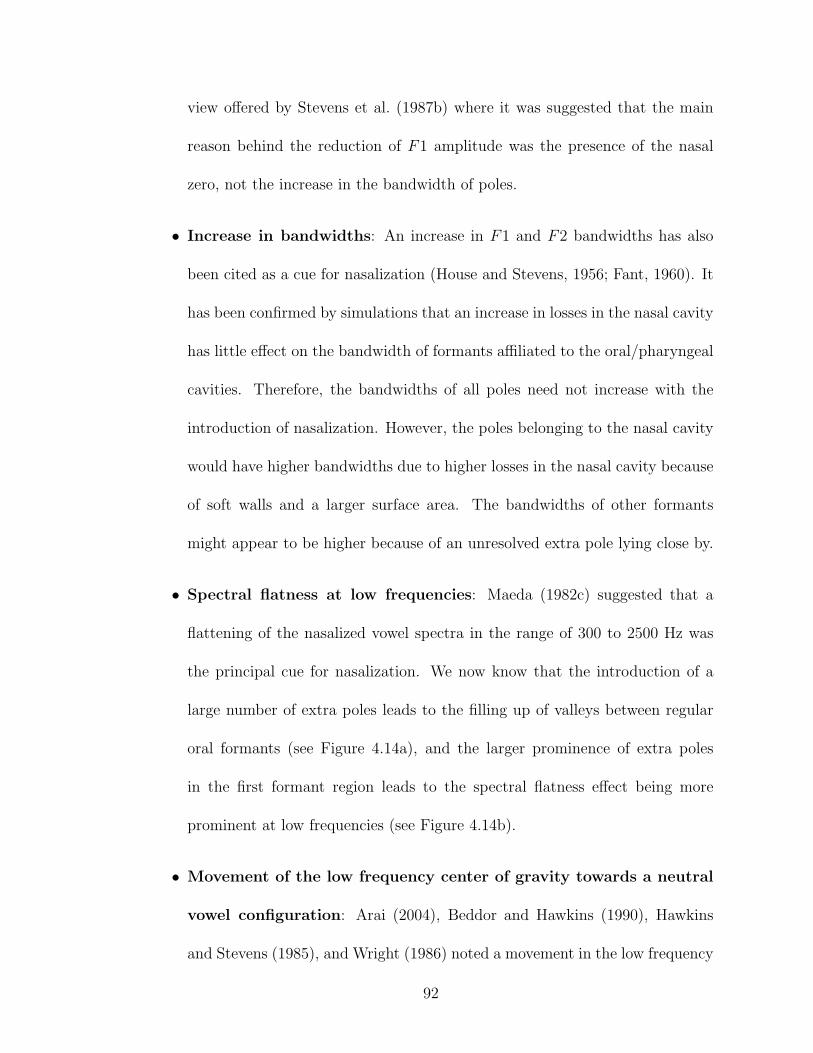
view offered by Stevens et al. (1987b) where it was suggested that the main

reason behind the reduction of F1 amplitude was the presence of the nasal

zero, not the increase in the bandwidth of poles.

• Increase in bandwidths: An increase in F1 and F2 bandwidths has also

been cited as a cue for nasalization (House and Stevens, 1956; Fant, 1960). It

has been confirmed by simulations that an increase in losses in the nasal cavity

has little effect on the bandwidth of formants affiliated to the oral/pharyngeal

cavities. Therefore, the bandwidths of all poles need not increase with the

introduction of nasalization. However, the poles belonging to the nasal cavity

would have higher bandwidths due to higher losses in the nasal cavity because

of soft walls and a larger surface area. The bandwidths of other formants

might appear to be higher because of an unresolved extra pole lying close by.

• Spectral flatness at low frequencies: Maeda (1982c) suggested that a

flattening of the nasalized vowel spectra in the range of 300 to 2500 Hz was

the principal cue for nasalization. We now know that the introduction of a

large number of extra poles leads to the filling up of valleys between regular

oral formants (see Figure 4.14a), and the larger prominence of extra poles

in the first formant region leads to the spectral flatness effect being more

prominent at low frequencies (see Figure 4.14b).

• Movement of the low frequency center of gravity towards a neutral

vowel configuration: Arai (2004), Beddor and Hawkins (1990), Hawkins

and Stevens (1985), and Wright (1986) noted a movement in the low frequency

92

center of gravity towards a neutral vowel configuration with nasalization. The

analysis above has shown that this effect should be expected both for low

and high vowels, since, for low vowels extra poles are introduced below F1

(see Figure 4.14b), and for high vowels the extra poles above F1 increase in

prominence with nasalization (see Figure 4.14a). This would cause the low

frequency center of gravity for low vowels to decrease and for high vowels to

increase.

• Reduction in the overall intensity of the vowel: House and Stevens

(1956) observed an overall reduction in the amplitude of the vowel. This

reduction is most likely due to the presence of several zeros in the nasalized

vowel spectrum as shown in the simulations above.

• Shifts in pole frequencies: It must be remembered that the nasal cavity

is a large and complicated cavity, and also gives a volume velocity output.

Therefore, even a tiny amount of coupling between the oral and nasal cavities

can introduce large changes in the spectrum. Poles can suddenly switch their

affiliation from the oral cavity to the nasal cavity. Thus, some of the prominent

poles might now be affiliated to the nasal cavity instead of the oral cavity. It

might as well be these nasal poles which seem to be moving in frequency.

Further, this effect need not be limited only to the low frequency poles. As

seen in the simulations in this study, even F2 and F3 might also change

significantly. Such shifts in formant frequencies have been observed in the

past by Bognar and Fujisaki (1986), Dickson (1962) and Hawkins and Stevens

93

(1985).

Given this detailed understanding of the spectral consequences of nasalization,

possible APs for the automatic detection of vowel nasalization will now be proposed.

94

Chapter 5

Acoustic Parameters

This chapter presents an exhaustive list of the various Acoustic Parameters

(APs) which have been proposed in this study to discriminate oral vowels from

nasalized vowels. It also gives detailed descriptions of the algorithms used to extract

these APs automatically. All of these APs were based on the knowledge gained

about the acoustic characteristics of nasalization through literature survey, acoustic

analysis, and vocal tract modeling. This chapter also presents a detailed description

of the procedure used to select a small number of efficient and relatively uncorrelated

APs from the complete set. Note that all the box and whisker plots presented in this

chapter are based on oral and nasalized vowels extracted from the TIMIT training

database according to the criteria described in Section 3.1.2. Tables for the mean

values of all of the proposed APs along with the F-ratios obtained from Analysis of

Variance (ANOVA) are also shown for the training sets of StoryDB and WS96/97.

5.1 Proposed APs

5.1.1 Acoustic correlate: Extra poles at low frequencies.

The literature survey and the vocal tract modeling study have shown that one

of the most important and stable properties of nasalization is the introduction of

extra poles in the F1 region. The parameters proposed in this section try to capture

95

the changes in spectral properties of vowels due to these extra poles.

5.1.1.1 A1− P0, A1− P1, F1− Fp0, F1− Fp1

Chen (1995, 1997) proposed the two parameters A1−P0 and A1−P1, where

A1 is the amplitude of the first formant, P0 is the amplitude of an extra nasal pole

below the first formant, and P1 is the amplitude of an extra nasal pole above the

first formant.

It was suggested that A1 − P0 would capture the reduction in A1 and the

increase in P0 which is introduced because of coupling to the paranasal sinuses,

whereas A1−P1 would capture the reduction in A1, and the increase in P1 because

of an increase in velopharyngeal opening. The vocal tract modeling study presented

in Chapter 4 has confirmed that nasalization leads to the introduction of an extra

pole (P0) due to the maxillary sinuses at a frequency around 500 Hz, and an extra

pole due to nasal coupling (P1) at frequencies around 1000 Hz (see Figure 4.14).

P0 was found to occur at a frequency below F1 for the low vowel /aa/ and above

F1 for the high vowel /iy/. It was also observed that both P0 and P1 increase in

frequency and prominence with increasing coupling area. Further, P0 was found to

be more prominent for /aa/, whereas P1 was found to be more prominent for /iy/.

Thus, both A1− P0 and A1− P1 are expected to have smaller values for nasalized

vowels.

Chen also proposed a modification of these parameters to make them indepen-

dent of vowel context by replacing A1 − P0 by A1 − P0 − T1(Fp0) − T2(Fp0) and

96

A1− P1 by A1− P1− T1(Fp1)− T2(Fp1) where:

T1(f) =(0.5B1)2 + F12√

[((0.5B1)2 + (F1− f)2)× ((0.5B1)2 + (F1 + f)2)](5.1)

T2(f) =(0.5B2)2 + F22√

[((0.5B2)2 + (F2− f)2)× ((0.5B2)2 + (F2 + f)2)](5.2)

Fp0 = frequency of the extra nasal pole below the first formant

Fp1 = frequency of the extra nasal pole above the first formant

B1 = bandwidth of the first formant

B2 = bandwidth of the second formant

T1(f) = effect of the first formant on the spectral amplitude at frequency f

T2(f) = effect of the second formant on the spectral amplitude at frequency f

Further, Maeda (1993, Page 160) proposed the use of the difference in fre-

quency between the first formant and Fp1 (F1− Fp1) to capture the increase in Fp1

with an increase in the velar coupling area. Another AP, F1− Fp0, has been added

in this work to capture the increase in Fp0 with increasing coupling area. Thus, the

proposed AP abs(F1 − Fp1) is expected to have larger values for nasalized vowels,

while abs(F1− Fp0) is expected to have smaller values for nasalized vowels.

Neither Chen nor Maeda proposed an automatic procedure to extract such

APs. An attempt to automate the extraction of the APs proposed by Chen was

made by Hajro (2004), but it met with limited success. There are two problems

with extracting these APs automatically:

1. It is very difficult to estimate A1 and to distinguish between F1 and the extra

poles due to the nasal cavity without knowing the value of F1.

97

2. It is very difficult to isolate these extra poles in the spectral domain automat-

ically because of (a) proximity to F1 leading to problems of resolution, (b)

presence of zeros leading to a reduction in the amplitude of these poles, and

(c) the harmonic structure of vowels (i.e., energy only at discrete frequencies).

These problems have been handled in this study in the following manner:

1. The best method to get F1 is to use an automatic formant tracker. In this

work, the ESPS formant tracker (Talkin, 1987) was used to get an estimate of

the first two formant frequencies and their bandwidths (with a 30 ms hanning

window and a shift of 5 ms). The formant tracker is likely to make some errors.

However, without knowing F1 it is almost impossible to decide which peaks

in the spectrum should be considered as oral formants and which ones should

be considered as extra nasal poles. The performance of the ESPS formant

tracking algorithm (which is also used in the open source tool WaveSurfer)

was recently evaluated by Deng et al. (2006) by comparing the F1/F2/F3

tracks obtained by this algorithm against a hand-corrected database of formant

tracks. Results of this study suggested that the ESPS formant tracker is very

accurate in the vowel regions for both F1 and F2. Note that, this study did

not break down the results for vowels into oral vowels and nasalized vowels.

Therefore, the results for vowels are an average of the results for both oral and

nasalized vowels. Further, to minimize the effect of errors in formant tracking

on the performance of the APs, the following procedure was used:

(a) Instead of directly using F1 and F2 obtained from the formant tracker,

98

the proposed algorithm first finds the frequencies of the peaks in a narrow-

band spectrum which are closest to the F1, F2 returned by the formant

tracker, and uses those frequencies as F1, F2.

(b) F2 is likely to have more errors than F1 (Deng et al., 2006). Therefore,

F2 is not used as an AP. It is only used as a guide to limit the search for

extra poles.

2. As discussed in Section 2.3, Group delay has been shown to have a much

better ability to identify closely spaced poles as compared to FFT because

of the additive property of phase (Yegnanarayana, 1978; Vijayalakshmi and

Reddy, 2005b). Further, the modified group delay function has been shown

to be effective in the detection of hypernasality by Vijayalakshmi and Reddy

(2005a). Thus, the modified group delay spectrum was used in this study in

addition to the cepstrally smoothed spectrum to get these APs.

Five different sets of these four parameters (A1−P0, A1−P1, F1−Fp0, and

F1− Fp1) were extracted. The five sets were extracted from:

1. Cepstrally smoothed FFT spectrum of the speech signal passed through a

preemphasis filter (H(z) = 1 − 0.97z−1). The preemphasis filter effectively

removes the glottal tilt from the spectrum which can reduce the amplitude

of the extra nasal pole above F1. The spectral frames were calculated once

every 5 ms with a hanning window of duration 30 ms and FFT size of 1024.

Every frame of speech was first normalized with the maximum amplitude in

that frame before the calculation of the spectra, and cepstral smoothing was

99

done by using a rectangular liftering window of length 3 ms. The names of

these four APs will be prefixed by an ’s’.

2. Same as case 1 except that in this case the parameters A1− P0 and A1− P1

were also normalized for vowel type by the procedure suggested by Chen. The

names of these four APs will be prefixed by an ’ns’.

3. Cepstrally smoothed modified group delay spectrum of the speech signal ex-

tracted as per Equations 2.1 and 2.2. The speech signal was not passed through

the preemphasis filter in this case because group delay removes the glottal tilt.

Here also, cepstral smoothing was performed by using a rectangular liftering

window of length 3 ms. The names of these four APs will be prefixed by a ’g’.

4. A combination of cepstrally smoothed FFT spectrum and modified group de-

lay spectrum. In cases where default values were assigned when the extra poles

were extracted from the FFT spectrum, the modified group delay spectrum

was used to locate the extra poles. If extra poles were found in the modified

group delay spectrum, then the frequencies of the harmonics in the FFT spec-

trum which were closest to those pole frequencies were used as Fp0 and Fp1,

and P0 and P1 were extracted from the FFT spectrum by getting the spectral

amplitudes at these frequencies. This is helpful in the cases where the group

delay spectrum is able to resolve the poles when the FFT spectrum does not.

The names of these four APs will be prefixed by an ’sg’.

5. Same as case 4 except that in this case the parameters A1− P0 and A1− P1

100

were also normalized for vowel type by the procedure suggested by Chen. The

names of these four APs will be prefixed by a ’nsg’.

The algorithm used to identify P0 and P1, and calculate the four APs de-

scribed above is provided in Appendix C. This algorithm describes the procedure

used for one single frame of a segment. Hence, it is repeated for all the frames in

the segment. The same procedure is used for both cepstrally smoothed spectra and

the modified group delay based spectra. However, the group delay spectra are not

log spectra. Therefore, when using the group delay spectra A1/P0 and A1/P1 are

used to calculate the APs instead of A1− P0 and A1− P1. However, the APs will

always be referred to as A1− P0 and A1− P1 in the description.

Figures 5.1-5.5 show the box and whisker plots for all 20 of the APs for the

TIMIT training database. These figures also show the normalized F-ratios obtained

through ANOVA for each of the APs. The normalization of the F-ratios was done

by dividing F by the total degrees of freedom (= number of samples + 1). This

normalization enables us to compare the F-ratios for different databases with dif-

ferent degrees of freedom. The normalized F-ratios will, henceforth, be referred to

as simply ”F” or ”F-values/ratios”. As expected, the values for A1− P0, A1− P1

and F1 − Fp0 are smaller on average for nasalized vowels, however, the values for

F1 − Fp1 are also smaller for nasalized vowels which is the opposite of what was

expected. This happens most likely because even though Fp1 is expected to increase

with increasing coupling area, F1 would also increase and the difference can actually

be smaller.

101

(a) sA1− P0 (b) sA1− P1

(c) sF1− Fp0 (d) sF1− Fp1

Figure 5.1: Box and whisker plots for the first set of four APs based on Cepstrallysmoothed FFT Spectrum.

102

(a) nsA1− P0 (b) nsA1− P1

(c) nsF1− Fp0 (d) nsF1− Fp1

Figure 5.2: Box and whisker plots for the second set of four APs based on Cepstrallysmoothed FFT Spectrum with normalization.

103

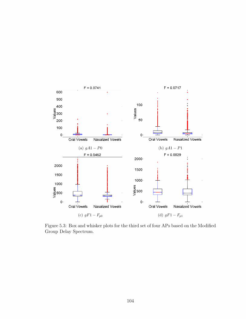
(a) gA1− P0 (b) gA1− P1

(c) gF1− Fp0 (d) gF1− Fp1

Figure 5.3: Box and whisker plots for the third set of four APs based on the ModifiedGroup Delay Spectrum.

104

(a) sgA1− P0 (b) sgA1− P1

(c) sgF1− Fp0 (d) sgF1− Fp1

Figure 5.4: Box and whisker plots for the fourth set of four APs based on a com-bination of the Cepstrally smoothed FFT Spectrum and the Modified Group DelaySpectrum.

105

(a) nsgA1− P0 (b) nsgA1− P1

(c) nsgF1− Fp0 (d) nsgF1− Fp1

Figure 5.5: Box and whisker plots for the fifth set of four APs based on a combinationof the Cepstrally smoothed FFT Spectrum and the Modified Group Delay Spectrumwith normalization.

106

5.1.1.2 teF1, teF2

The vocal tract modeling study has shown that the low frequency spectra of

nasalized vowels can have a multitude of poles due to nasal coupling and due to the

paranasal sinuses. Thus, the teager energy operator which was used by Cairns et al.

(1994, 1996b,a) for the detection of hypernasality may prove to be useful. However,

as discussed in Section 2.3, the limitations in the study by Cairns et al make it

too restrictive for generalized applications across all vowels. Further, this study

used pitch synchronous analysis which is an extremely specialized and complicated

algorithm, and therefore may complicate the extraction of APs based on teager

energy. It is proposed that most of these restrictions be discarded and instead of

using the correlation between the teager energy profiles of lowpass filtered speech

and bandpass filtered speech, the correlation between the teager energy profiles of

narrow bandpass filtered speech and wide bandpass filtered speech centered around

two different frequency regions be considered. In this case, the frequency regions

were centered around the first two formant frequencies obtained from the formant

tracker.

The teager energy profile, Ψd[x(n)], for a signal x(n) is calculated as:

Ψd[x(n)] = x2(n)− x(n + 1)x(n− 1) (5.3)

Thus, the proposed APs based on teager energy profile were calculated as:

teF1 = ρ(Ψd[sNBF1], Ψd[sWBF1]) (5.4)

teF2 = ρ(Ψd[sNBF2], Ψd[sWBF2]) (5.5)

107

(a) teF1 (b) teF2

Figure 5.6: Box and whisker plots for teF1 and teF2.

sNBF1/F2 = Narrowband filtered speech signal centered around F1/F2.

sWBF1/F2 = Wideband filetered speech signal centered around F1/F2.

A bandwidth of 100 Hz was used for the narrowband filter, and the bandwidth

of the wideband filter was set to 1000 Hz. The filters were implemented with the

MATLAB command fir1 with a filter order of 200. Box and whisker plots for the

two APs for TIMIT training database are shown in Figure 5.6. As expected, the

correlation values are smaller on average for nasalized vowels for teF1. However,

there is hardly any difference between the correlation values for oral and nasalized

vowels for teF2.

5.1.1.3 E(0− F2), nE(0− F2)

The presence of a number of extra poles at low frequencies should also give a

boost to the energy of nasalized vowel spectra at low frequencies. Thus, two energy

based parameters, E(0−F2) and nE(0−F2), have also been proposed in this study

108

(a) E(0− F2) (b) nE(0− F2)

Figure 5.7: Box and whisker plots for E(0− F2) and nE(0− F2).

to capture the contribution of the extra poles in the low frequency region to spectral

energy. The first parameter E(0− F2) is calculated as:

E(0− F2) =En(0− F2)

(En(0− fs/2) ∗ F2)(5.6)

where fs = sampling rate, En(0− F2) gives the spectral energy between 0 Hz and

F2, and En(0− fs/2) gives the spectral energy between 0 Hz and fs/2. The nor-

malization by En(0−fs/2) was done to remove the dependency on the total energy

in the frame, and the normalization by F2 was done to remove the dependence on

the variable F2 for different vowels. To calculate nE(0 − F2), the contribution of

F1 and F2 was first subtracted from the total energy by the procedure suggested

by Chen before evaluating the parameter as per the method described above for

the first parameter. This was done in order to emphasize the contribution of the

extra nasal poles to the spectral energy. Box plots of E(0 − F2) and nE(0 − F2)

are shown in Figure 5.7. As can be seen from the figures, these APs were not very

useful for the distinction between oral and nasalized vowels.

109

5.1.2 Acoustic correlate: Extra poles and zeros across the spectrum.

The vocal tract modeling study has shown that extra poles and zeros are

introduced in the nasalized vowel spectrum not just at low frequencies, but across

the whole frequency spectrum. Further, Stevens (1998, Page 189) had suggested

that the total number of poles in the vocal tract transfer function up to a certain

frequency f can be approximated by np = 2ltf/c where lt is the total length of all

of the tube components in the model, including side branches and parallel branches.

Thus, the density of poles in nasalized vowel spectra due to the combined vocal

tract and nasal tract along with the paranasal sinuses is expected to be much higher

than that for oral vowels. The APs proposed in this section, therefore, attempt to

capture this information. Note that, all the APs proposed in this section are based

on the the cepstrally smoothed log magnitude FFT spectrum extracted by using the

same constants as described in Section 5.1.1.1. The only difference is that in this

case, speech was not passed through a high pass filter before calculating the spectra.

5.1.2.1 nDips, avgDipAmp, maxDipAmp

Since nasalization introduces a lot of extra poles in the spectrum which fill up

the valleys between oral formants, it should be expected that nasalized vowels would

have a larger number of dips in the spectrum, and that on an average dips would be

less strong for nasalized vowels. The dip amplitudes can be obtained by capturing

the peaks in the difference of the amplitude of the convex hull (Mermelstein, 1975)

of the magnitude spectrum and the spectrum itself. Therefore, the following APs

110

were proposed to capture this information:

nDips = number of dips between 0-4000 Hz of the Cepstrally smoothed FFT spec-

trum.

avgDipAmp = (∑

all dips in 0-4000Hz dip amplitudes)/nDips.

maxDipAmp = maxall dips in 0-4000Hz dip amplitudes.

The limit of 4000 Hz was proposed to accommodate telephone bandwidth speech

without any modifications. Box and whisker plots for the three APs for TIMIT

training database are shown in Figure 5.8. As expected, nasalized vowels have a

larger number of dips and lower dip amplitudes on average. However, the maximum

dip amplitude is larger for nasalized vowels on average, which is most probably due

to the presence of zeros in the spectra of nasalized vowels.

5.1.2.2 std0− 1K, std1K − 2K, std2K − 3K, std3K − 4K

A parameter to capture the standard deviation in frequency around the center

of mass of the low frequency region was proposed by Glass (1984) and Glass and

Zue (1985). This parameter can potentially capture the diffuse nature of a nasalized

vowel spectrum along with the reduction in F1 amplitude, increase in bandwidth of

low frequency poles and spectral flatness at low frequencies. However, this diffuse

nature of the nasalized vowel spectrum is also present at higher frequencies because

of the extra nasal poles and the increase in losses due to the soft walls of the nasal

cavity, even though the effect is much less pronounced at higher frequencies. There-

fore, it is proposed that such standard deviation values be calculated around four

111

(a) nDips (b) avgDipAmp

(c) maxDipAmp

Figure 5.8: Box and whisker plots for nDips, avgDipAmp and maxDipAmp.

112

center frequencies spread over the entire frequency range. Thus, the following APs

have been used:

std0− 1K = standard deviation around the center of mass in 0-1000 Hz.

std1K − 2K = standard deviation around the center of mass in 1000-2000 Hz.

std2K − 3K = standard deviation around the center of mass in 2000-3000 Hz.

std3K − 4K = standard deviation around the center of mass in 3000-4000 Hz.

To calculate the center of mass in a band, any amplitude value less than the

threshold (= 20dB below the maximum in the band under consideration) was made

equal to the threshold, and then the threshold was subtracted from all the values in

the frame to set the floor to zero. A trapezoidal window which is flat betwee 100-

900 Hz (for the first band, and similarly for the other bands) was then applied to

the selected band to reduce the sensitivity of the center of mass to sudden changes

at the end points of the band. The standard deviation was then calculated in a

frequency radius of 500 Hz around the center of mass in that band. However, the

upper and lower limits for the standard deviation calculation were limited by the

frequency range of each band. Therefore, if the center of mass in the second band

was at 1300 Hz, then the standard deviation was calculated by looking at a band

of 1000-1800 Hz. The standard deviation thus calculated was scaled by the ratio of

the maximum frequency width (i.e. 1000 Hz) to the actual frequency width used to

remove the dependence on the frequency width. This procedure is very similar to

that used by Glass (1984).

Box and whisker plots for these four APs for TIMIT training database are

113

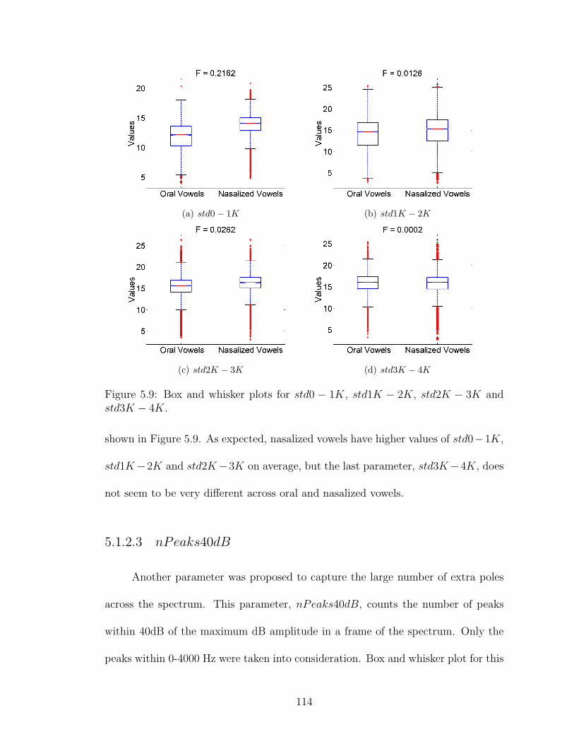
(a) std0− 1K (b) std1K − 2K

(c) std2K − 3K (d) std3K − 4K

Figure 5.9: Box and whisker plots for std0 − 1K, std1K − 2K, std2K − 3K andstd3K − 4K.

shown in Figure 5.9. As expected, nasalized vowels have higher values of std0−1K,

std1K−2K and std2K−3K on average, but the last parameter, std3K−4K, does

not seem to be very different across oral and nasalized vowels.

5.1.2.3 nPeaks40dB

Another parameter was proposed to capture the large number of extra poles

across the spectrum. This parameter, nPeaks40dB, counts the number of peaks

within 40dB of the maximum dB amplitude in a frame of the spectrum. Only the

peaks within 0-4000 Hz were taken into consideration. Box and whisker plot for this

114

Figure 5.10: Box and whisker plot for nPeaks40dB.

AP is shown in Figure 5.10. As expected, nasalized vowels have a larger number of

peaks on average.

5.1.3 Acoustic correlate: F1 amplitude reduction.

5.1.3.1 a1− h1max800, a1− h1fmt

Huffman (1990) identified the average value of A1 − H1 (i.e. the difference

between the amplitude of the first formant and the first harmonic), and change in

A1−H1 over time as being correlated to the perception of nasality. A reduction in

A1−H1 is expected because A1 reduces with nasalization (as was also confirmed in

the simulations in Chapter 4), and H1 stays almost constant (Stevens, 1998, Page

489). This can be easily extracted by subtracting the amplitude of the first har-

monic in the spectrum from an estimate of A1. In this thesis, two different methods

of estimating A1 were evaluated. Thus,

a1 − h1max800 = A1 − H1, where A1 is estimated by using the amplitude of the

115

(a) a1− h1max800 (b) a1− h1fmt

Figure 5.11: Box and whisker plots for a1− h1max800 and a1− h1fmt.

maximum value in 0-800 Hz.

a1− h1fmt = A1−H1, where A1 is estimated by using the amplitude of the peak

closest to the F1 obtained by using the ESPS formant tracker.

H1 was obtained by using the amplitude of the peak closest to 0 Hz which had

a height greater than 10dB and a width greater than 80 Hz. These thresholds were

obtained empirically. The width of the peak was estimated as the difference between

the frequencies of the first dip after the peak and the last dip before the peak. The

height of the peak was estimated as the sum of the differences between the peak

and the two surrounding dips. Also note that the amplitudes and frequencies of the

peaks for the calculation of H1 were extracted from the narrowband FFT spectrum

evaluated with the same constants as described in Section 5.1.1.1. Box and whisker

plots for a1 − h1max800 and a1 − h1fmt are shown in Figure 5.11. As expected,

A1−H1 is found to be smaller on average for nasalized vowels as compared to oral

vowels.

116

(a) slope0− 1500

Figure 5.12: Box and whisker plots for slope0− 1500.

5.1.4 Acoustic correlate: Spectral flattening at low frequencies.

5.1.4.1 slope0− 1500

Maeda (1982a) and Maeda (1993)[Page 160] had proposed the importance of

spectral flattening in the low frequency regions as a cue for vowel nasalization. The

simulations shown in Chapter 4 suggested that the introduction of a large number

of extra poles leads to the filling up of valleys between regular oral formants, and

the larger prominence of extra poles in the first formant region leads to the spectral

flatness effect being more prominent at low frequencies. It is proposed that the slope

of a linear least squares fit to the Cepstrally smoothed FFT spectrum in the range

of 0-1500 Hz be used as a parameter for the purpose. Thus, the slope is expected

to be steeper for oral vowels as compared to nasalized vowels. Box and whisker plot

for slope0 − 1500 is shown in Figure 5.12. As expected, the average value of the

slope is slightly smaller for nasalized vowels as compared to oral vowels. However,

the difference is not too large.

117

(a) F1BW (b) F2BW

Figure 5.13: Box and whisker plots for F1BW and F2BW .

5.1.5 Acoustic correlate: Increase in bandwidths of formants.

5.1.5.1 F1BW , F2BW

As was discussed in Chapter 2, several researchers in the past have observed

a widening of F1 and F2 bandwidth with the introduction of nasalization. The

simulations in Chapter 4 suggested that even though the bandwidths of oral formants

may not increase due to the losses in the nasal cavity, the bandwidths of these

formants may appear to be wider because of unresolved poles which appear at

frequencies very close to these oral formants. A measure of F1 and F2 bandwidths

obtained from the ESPS formant tracker was used in this thesis. Box and whisker

plots for F1BW and F2BW are shown in Figure 5.13. As expected, the bandwidth

of F1 was found to be significantly larger for nasalized vowels as compared to oral

vowels. However, not much of a difference was observed in the bandwidth of F2.

118

Table 5.1: F-ratios for the 5 sets of A1− P0, A1− P1, F1− Fp0, F1− Fp1.

Label StoryDB TIMIT WS96/97

sA1− P0 0.2384 0.1413 0.0531

sA1− P1 0.1437 0.0782 0.0070

sF1− Fp0 0.0082 0.0319 0.0008

sF1− Fp1 0.0238 0.0013 0.0373

nsA1− P0 0.4258 0.0407 0.1420

nsA1− P1 0.0388 0.0353 0.0803

nsF1− Fp0 0.0082 0.0319 0.0008

nsF1− Fp1 0.0238 0.0013 0.0373

gA1− P0 0.1083 0.0741 0.0000

gA1− P1 0.0292 0.0717 0.0004

gF1− Fp0 0.0011 0.0462 0.0008

gF1− Fp1 0.0558 0.0029 0.0350

sgA1− P0 0.3414 0.2045 0.1062

sgA1− P1 0.1930 0.0854 0.0080

sgF1− Fp0 0.0260 0.0391 0.0044

sgF1− Fp1 0.0523 0.0020 0.0379

nsgA1− P0 0.3808 0.0555 0.1664

nsgA1− P1 0.0332 0.0361 0.0830

nsgF1− Fp0 0.0260 0.0391 0.0044

nsgF1− Fp1 0.0523 0.0020 0.0379

119

5.2 Selection of APs

Since the five different sets of A1 − P0, A1 − P1, F1 − Fp0 and F1 − Fp1

essentially capture the same information, only the best set of these 4 APs (the ’sg’

set) was selected based on the highest normalized F-ratios. F-ratios for the APs are

shown in Table 5.1 for StoryDB, TIMIT and WS96/97. The mean values for all of

the APs for the two categories of oral and nasalized vowels are also shown in Table

5.2 for comparison purposes. Figure 5.14 plots the F-ratios shown in Table 5.1 for

StoryDB, TIMIT and WS96/97 as a percentage of the total of the F-ratios in each

column of Table 5.1. Based on this figure, the fourth set of these 4 APs (sgA1−P0,

sgA1 − P1, sgF1 − Fp0 and sgF1 − Fp1) was selected for further processing since

that set of APs consistently performed the best across the three databases (see the

boxed region in Figure 5.14).

F-ratios for the above set of 4 APs along with the rest of the APs are shown

in Table 5.3 for StoryDB, TIMIT and WS96/97. The mean values for all of the

proposed APs for oral and nasalized vowels are also shown in Table 5.4 for StoryDB,

TIMIT and WS96/97. Figure 5.15 plots the F-ratios shown in Table 5.3 for StoryDB,

TIMIT and WS96/97 as a percentage of the total of the F-ratios in each column.

The APs that were selected for further processing are highlighted by red boxes. The

selection was based on the following criterion: If any of the APs performed extremely

poorly for at least one of the databases, then it was not selected. Thus, according to

this criterion 9 out of the total of 37 proposed APs were selected (see the boxed APs

in Figure 5.15). This set of 9 APs will be used in the next Chapter to automatically

120

classify oral and nasalized vowels.

Table 5.2: Mean values for the 5 sets of A1− P0, A1− P1, F1− Fp0, F1− Fp1.

StoryDB TIMIT WS96/97

Label Oral Nasalized Oral Nasalized Oral Nasalized

sA1− P0 21.85 12.73 15.93 10.97 13.36 9.65

sA1− P1 21.32 14.31 11.34 8.04 10.54 9.35

sF1− Fp0 476.77 437.60 471.57 397.23 416.02 402.58

sF1− Fp1 602.17 515.39 434.47 419.56 465.38 559.34

nsA1− P0 16.27 9.11 14.18 10.92 12.63 6.16

nsA1− P1 11.75 8.25 10.22 7.03 7.43 0.97

nsF1− Fp0 476.77 437.60 471.57 397.23 416.02 402.58

nsF1− Fp1 602.17 515.39 434.47 419.56 465.38 559.34

gA1− P0 13.70 3.32 8.53 3.60 6.02 6.13

gA1− P1 10.76 7.28 10.88 6.62 4.24 3.49

gF1− Fp0 434.29 421.49 487.38 383.18 426.07 440.17

gF1− Fp1 671.35 536.16 486.73 465.12 514.45 602.30

sgA1− P0 20.51 11.49 16.71 10.84 14.98 9.64

sgA1− P1 21.01 13.74 11.41 7.97 10.26 9.02

sgF1− Fp0 453.51 395.97 445.90 371.99 416.30 388.62

sgF1− Fp1 649.21 520.58 445.23 427.05 481.67 575.92

Continued on next page

121

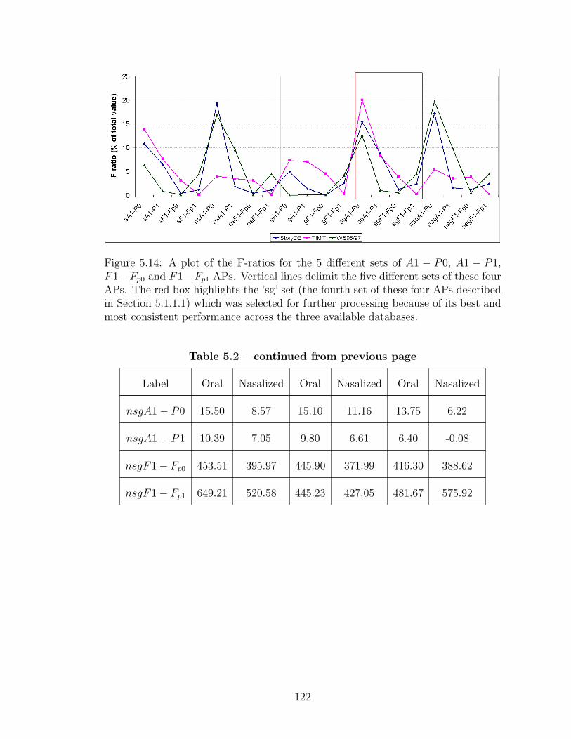
Figure 5.14: A plot of the F-ratios for the 5 different sets of A1 − P0, A1 − P1,F1−Fp0 and F1−Fp1 APs. Vertical lines delimit the five different sets of these fourAPs. The red box highlights the ’sg’ set (the fourth set of these four APs describedin Section 5.1.1.1) which was selected for further processing because of its best andmost consistent performance across the three available databases.

Table 5.2 – continued from previous page

Label Oral Nasalized Oral Nasalized Oral Nasalized

nsgA1− P0 15.50 8.57 15.10 11.16 13.75 6.22

nsgA1− P1 10.39 7.05 9.80 6.61 6.40 -0.08

nsgF1− Fp0 453.51 395.97 445.90 371.99 416.30 388.62

nsgF1− Fp1 649.21 520.58 445.23 427.05 481.67 575.92

122

Table 5.3: F-ratios for all the proposed APs for StoryDB, TIMIT and WS96/97.

Label StoryDB TIMIT WS96/97

sgA1− P0 0.3414 0.2045 0.1062

sgA1− P1 0.1930 0.0854 0.0080

sgF1− Fp0 0.0260 0.0391 0.0044

sgF1− Fp1 0.0523 0.0020 0.0379

teF1 0.0578 0.0726 0.0224

teF2 0.0437 0.0000 0.0048

std0− 1K 0.0641 0.2162 0.0158

std1K − 2K 0.0039 0.0126 0.0134

std2K − 3K 0.0620 0.0262 0.0001

std3K − 4K 0.0077 0.0002 0.0035

nDips 0.0020 0.0252 0.0077

avgDipAmp 0.0000 0.0001 0.0002

maxDipAmp 0.0029 0.0234 0.0000

nPeaks40dB 0.0975 0.0466 0.0143

slope0− 1500 0.0223 0.0016 0.0235

a1− h1max800 0.3049 0.1507 0.0847

a1− h1fmt 0.5456 0.0977 0.0703

F1BW 0.4239 0.2648 0.0412

F2BW 0.0009 0.0082 0.0282

E(0− F2) 0.0000 0.0080 0.0117

nE(0− F2) 0.0179 0.0043 0.0143

123

Table 5.4: Mean values for all the proposed APs for StoryDB, TIMIT and WS96/97.

StoryDB TIMIT WS96/97

Label Oral Nasalized Oral Nasalized Oral Nasalized

sgA1− P0 20.51 11.49 16.71 10.84 14.98 9.64

sgA1− P1 21.01 13.74 11.41 7.97 10.26 9.02

sgF1− Fp0 453.51 395.97 445.90 371.99 416.30 388.62

sgF1− Fp1 649.21 520.58 445.23 427.05 481.67 575.92

teF1 0.69 0.65 0.60 0.54 0.54 0.50

teF2 0.56 0.61 0.52 0.52 0.47 0.45

std0− 1K 11.52 13.34 11.92 13.83 24.70 26.11

std1K − 2K 13.49 13.89 13.81 14.68 29.66 31.05

std2K − 3K 15.11 16.39 15.28 16.11 31.35 31.43

std3K − 4K 16.12 15.88 15.72 15.65 30.41 31.02

nDips 5.92 6.02 6.40 6.83 6.89 7.15

avgDipAmp 13.30 13.23 9.62 9.55 8.50 8.60

maxDipAmp 23.66 24.63 17.41 19.30 16.62 16.69

nPeaks40dB 5.80 6.74 6.93 7.58 7.50 7.86

slope0− 1500 0.02 0.01 0.01 0.01 0.01 0.01

a1− h1max800 7.72 4.14 16.58 11.48 15.18 9.34

a1− h1fmt 7.50 1.41 14.73 7.83 11.51 3.49

Continued on next page

124

Figure 5.15: A plot of the F-ratios for sgA1 − P0, sgA1 − P1, sgF1 − Fp0 andsgF1 − Fp1 along with the rest of the proposed APs. The red boxes highlight thenine APs which were selected for use as the knowledge-based APs for the automaticdetection of vowel nasalization.

Table 5.4 – continued from previous page

Label Oral Nasalized Oral Nasalized Oral Nasalized

F1BW 93.43 193.28 89.13 172.14 124.74 170.51

F2BW 145.94 152.30 150.13 169.05 198.62 263.36

E(0− F2) -20.38 -20.39 -20.44 -20.68 -23.44 -23.10

nE(0− F2) -60.41 -58.15 -60.15 -61.06 -48.82 -50.87

5.3 Chapter Summary

This chapter presented an exhaustive list of the APs proposed in this thesis

to discriminate oral vowels from nasalized vowels. A total of 37 APs were proposed

in this chapter. All of these APs were based on the knowledge gained about the

125

acoustic characteristics of nasalization through literature survey, acoustic analysis,

and vocal tract modeling. A detailed discussion of the ideology behind each of the

APs was presented in this chapter along with the implementation details. It is

clear from the figures in this chapter, that some of the APs were not very good at

discriminating oral and nasalized vowels. However, documenting all the APs that

were tried has the benefit of acting as a reference for the future, so that additional

effort is not spent on trying similar APs again.

Out of this set of 37 APs, 9 APs with the best normalized F-ratios (obtained

from ANOVA) were selected for further use. The selected APs are: (1) sgA1− P0,

(2) sgA1 − P1, (3) sgF1 − Fp0, (4) teF1, (5) std0 − 1K, (6) nPeaks40dB, (7)

a1 − h1max800, (8) a1 − h1fmt, and (9) F1BW . The first four APs capture the

spectral changes due to the presence of extra nasal poles in nasalized vowels. The

fifth AP tries to capture the diffuse nature of nasalized vowel spectra along with the

reduction in F1 amplitude, increase in the bandwidth of low frequency poles and

spectral flatness at low frequencies. The sixth AP is a measure of the extra nasal

poles across the full range of frequencies in nasalized vowel spectra. The seventh

and eighth APs capture the reduction in F1 amplitude, and the last AP captures

the increase in the bandwidth of F1. These 9 APs will be used in the next chapter

to obtain results for the automatic detection of vowel nasalization.

126

Chapter 6

Results

This chapter presents the results obtained by using the proposed knowledge-

based APs in an SVM Classifier framework (as discusses in Section 3.3) to classify

oral and nasalized vowels. Results are presented for all the databases described

in Section 3.1 (i.e. StoryDB, TIMIT, WS96/97 and OGI). These results are also

compared to a set of baseline results to judge the improvement in performance

by using the proposed APs. This is followed by an extensive analysis of errors

to understand the sources of error and suggest possible improvements. Some of the

results presented in this chapter have also been presented in Pruthi and Espy-Wilson

(2006b).

6.1 Baseline Results

Results on APs proposed by Glass (1984) and Glass and Zue (1985) in the cur-

rent experimental setting are presented in this section since that was the only study

which directly approached the question of automatic detection of vowel nasalization.

The rest of the studies were either too restrictive for generalized application, or did

not extract the APs in an automatic manner. Also presented in this section are

results obtained in the WS04 JHU workshop (Hasegawa-Johnson et al., 2004, 2005),

and results on MFCCs in the current experimental setting. Thus, the complete set

127

of baseline results against which the performance of the APs proposed in this study

will be compared include the results obtained using MFCCs and the APs proposed

by Glass in the current experimental setting, and the results obtained during the

WS04 JHU workshop.

6.1.1 APs proposed by James Glass

In this experiment, considerable care was taken to follow the algorithm pro-

posed by Glass (1984) and Glass and Zue (1985) as closely as possible for a fair

comparison of the results obtained by using these APs and the results which will be

obtained later using the APs proposed in this study. Each oral or nasalized vowel

segment was divided into three equal subsegments, and a hamming window of size

25ms was used along with a frame shift of 5ms to get the spectrum amplitude. The

following parameters were then calculated:

1. Average value of the center of mass of the middle subsegment between fre-

quencies of 0 and 1000 Hz. Any amplitude values less than the threshold (=

maximum of the amplitude across all frames in the subsegment - 20) were

made equal to the threshold and then the threshold was subtracted from all

amplitude values to bring the floor to zero. Any frames with all values less

than threshold were neglected. A trapezoidal window flat between 100-900

Hz was then used with the rest of the frames to get the center of mass for

each frame. The values of the center of mass for all the frames in the middle

subsegment were averaged to get the average center of mass parameter.

128

2. Maximum value of the standard deviation in the three subsegments. Standard

deviation of frequency was calculated by using the spectral amplitudes 500 Hz

on each side of the center of mass for that frame. The low and high frequencies

were limited between 0 and 1000 Hz if they went below or over. The standard

deviation in each frame was multiplied by (1000/frequency range used for that

frame) to normalize for the frequency region used. The maximum value of the

average standard deviation in the three subsegments was then used as the AP.

3. Maximum percentage of time there is an extra resonance in three subsegments.

Smoothed spectra were first obtained for each frame by cepstral smoothing

with a cosine tapered lowpass window (flat for 1.5ms, and cosine tapered

for 1.5ms with a cosine of period 6ms). The first two peaks below 1000 Hz

are extracted for each frame from these smoothed spectra. If the first peak

is greater than 400 Hz, then the second peak for that frame is removed from

consideration and the resonance dip and resonance difference are set to zero. If,

however, the first peak is below 400 Hz, then the count for extra peaks for that

subsegment is incremented, and the resonance dip and resonance difference

are set to the difference between the amplitude of the minimum of the two

peaks and the minimum value in between the two peaks, and the difference

in amplitudes between the second peak and the first peak respectively. The

percentage of time there is an extra peak in a subsegment is calculated as the

ratio of number of frames with two peaks, and the total number of frames in

that subsegment. The maximum of these three values is then used as an AP.

129

(a) TIMIT (b) WS96/97

Figure 6.1: Plots showing the variation in cross-validation error with a change inthe number of segments/class used for training for a classifier using the gs6 set:(a) TIMIT, (b) WS96/97. The square dot marks the point with the least cross-validation error.

4. Minimum percentage of time there is an extra resonance in the three subseg-

ments. The minimum of three values obtained in the previous case is also used

as an AP.

5. Maximum value of the average dip between the first resonance and the extra

resonance in the three subsegments. Procedure described above.

6. Minimum value of the average difference between the first resonance and the

extra resonance in the three subsegments. Procedure described above.

This set of 6 APs will, henceforth, be referred to as the gs6 set. It should

be noted that these APs are segment based APs (i.e., only one set of 6 APs will be

obtained for the whole segment), not frame based. All the other results presented

in this chapter are based on APs which were extracted on a per frame basis. Also

note that results for StoryDB using these APs are not presented because the number

of oral vowel segments in this database were inadequate for proper training of the

classifier.

130

As described in Section 3.3.4, the training of the SVM classifier was done in

two passes. Plots of the % of Error with the different training set sizes used in the

first pass are shown in Figures 6.1a and 6.1b for TIMIT and WS96/97 databases

respectively. The point with the minimum cross-validation error is marked with a

square dot. The value on the x-axis at this point gives the number of samples per

class which should be used for training. Thus, in the second pass, this training set

size was used to select the training data and train SVM classifiers with both Linear

and RBF kernels.

Table 6.1: Classification results for oral vs nasalized vowels using the gs6 set. Train-ing database: TIMIT, Testing database: TIMIT.

% Correct (Linear) % Correct (RBF) Test Tokens

Oral Vowels 65.38 68.71 14136

Nasalized Vowels 77.84 76.24 4062

Chance Norm. Acc. 71.61 72.48 18198

Table 6.2: Classification results for oral vs nasalized vowels using the gs6 set. Train-ing database: WS96/97, Testing database: WS96/97.

% Correct (Linear) % Correct (RBF) Test Tokens

Oral Vowels 56.45 57.12 12373

Nasalized Vowels 62.82 64.16 1119

Chance Norm. Acc. 59.63 60.64 13492

Tables 6.1 and 6.2 present the results for TIMIT and WS96/97 databases

with Linear and RBF SVM classifiers, trained as described above, using the gs6 set.

131

These tables show that even though the performance of these APs is reasonably good

for TIMIT, it degrades significantly for the telephone speech database WS96/97.

6.1.2 Mel-Frequency Cepstral Coefficients

Mel-Frequency Cepstral Coefficients (MFCCs) are the standard set of front-

end parameters used in most of the state-of-the-art speech recognition systems.

Hence, a comparison to the results obtained by using these parameters in the cur-

rent experimental setting is worthwhile. The set of MFCCs used here included 12

MFCCs, energy, delta coefficients and acceleration coefficients, thus totalling to 39

coefficients. This set will, henceforth be referred to as the mf39 set. These coef-

ficients were generated once every 5ms with a 25ms hamming window. The source

waveform was normalized to zero mean before analysis and a preemphasis coefficient

of 0.97 was used. The LOFREQ and HIFREQ parameters were kept at their default

values (that is, 0-4000 Hz for WS96/97 and 0-8000 Hz for TIMIT). Cepstral mean

normalization was not used. Instead, the MFCCs were normalized to have a zero

mean and unit variance before being used for classification in SVMs.

Figure 6.2 plots the % of Error for different training set sizes used in the first

training pass to train Linear SVM classifiers for StoryDB, TIMIT and WS96/97

databases. Based on these plots, 1190 frames were used per class to train the SVMs

for StoryDB, 26000 frames/class were used for TIMIT and 1700 frames/class were

used for WS96/97. Tables 6.3-6.5 present the results for StoryDB, TIMIT and

WS96/97 using the mf39 set. It is clear from these tables that even though the

132

(a) StoryDB (b) TIMIT (c) WS96/97

Figure 6.2: Plots showing the variation in cross-validation error with a change inthe number of frames/class used for training for a classifier using the mf39 set: (a)StoryDB, (b) TIMIT, (c) WS96/97. The square dot marks the point with the leastcross-validation error.

chance normalized accuracies are very good, these results are highly skewed in favor

of correctly classifying the oral vowels, even though the same number of training

samples were used for both oral and nasalized vowel classes. For example, in Table

6.5, for the RBF SVM classifier, the accuracy for oral vowels is 80.13%, whereas the

accuracy for nasalized vowels is only 48.61%. Note that the accuracy for nasalized

vowels is even below the 50% chance accuracy for this task.

Table 6.3: Classification results for oral vs nasalized vowels using the mf39 set.Training database: StoryDB, Testing database: StoryDB.

% Correct (Linear) % Correct (RBF) Test Tokens

Oral Vowels 62.50 97.32 112

Nasalized Vowels 68.75 94.35 336

Chance Norm. Acc. 65.62 95.83 448

133

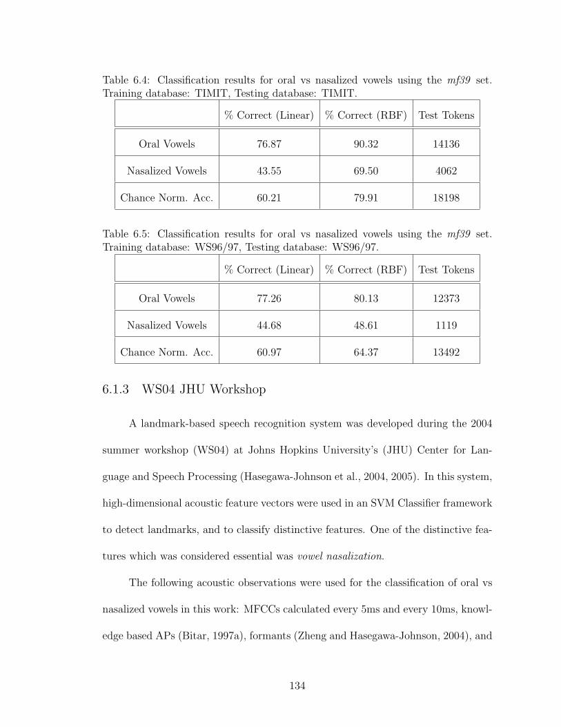
Table 6.4: Classification results for oral vs nasalized vowels using the mf39 set.Training database: TIMIT, Testing database: TIMIT.

% Correct (Linear) % Correct (RBF) Test Tokens

Oral Vowels 76.87 90.32 14136

Nasalized Vowels 43.55 69.50 4062

Chance Norm. Acc. 60.21 79.91 18198

Table 6.5: Classification results for oral vs nasalized vowels using the mf39 set.Training database: WS96/97, Testing database: WS96/97.

% Correct (Linear) % Correct (RBF) Test Tokens

Oral Vowels 77.26 80.13 12373

Nasalized Vowels 44.68 48.61 1119

Chance Norm. Acc. 60.97 64.37 13492

6.1.3 WS04 JHU Workshop

A landmark-based speech recognition system was developed during the 2004

summer workshop (WS04) at Johns Hopkins University’s (JHU) Center for Lan-

guage and Speech Processing (Hasegawa-Johnson et al., 2004, 2005). In this system,

high-dimensional acoustic feature vectors were used in an SVM Classifier framework

to detect landmarks, and to classify distinctive features. One of the distinctive fea-

tures which was considered essential was vowel nasalization.

The following acoustic observations were used for the classification of oral vs

nasalized vowels in this work: MFCCs calculated every 5ms and every 10ms, knowl-

edge based APs (Bitar, 1997a), formants (Zheng and Hasegawa-Johnson, 2004), and

134

rate-scale parameters (Mesgarani et al., 2004). The total dimensionality of this set

of APs was approximately 400. This set of APs will, henceforth, be referred to as the

WS04 set. The SVM classifier was trained with a linear kernel. Testing was done

on half of the WS96/97 corpus, and the other half was used for training purposes.

The division of the files into training and testing sets was done by alternating. In

reporting the accuracies, chance was normalized to 50%. Note that, in this case,

the task was to classify every frame into either oral or nasalized. Thus, these results

were frame-based results. An overall, chance normalized, frame-based accuracy of

62.96% was obtained in this study. Table 6.6 shows the classification results broken

down into the results for individual vowels.

6.2 Results from the APs proposed in this thesis

This section presents the results for the APs proposed in Chapter 5. For

comparison purposes, results for both the full set of 37 APs (henceforth referred to

as the tf37 set), and the set of 9 APs selected according to the procedure described

in Section 5.2 (henceforth referred to as the tf9 set), are presented in this section.

The best training set size for each of the three databases (StoryDB, TIMIT and

WS96/97) was selected individually for the tf37 and tf9 sets by training Linear

SVM classifiers and selecting the one which gave the least cross-validation error.

Figures 6.3 and 6.4 plot the variation in the % of Error with varying training set

sizes for the tf37 and tf9 sets respectively. Linear and RBF SVM classifiers were

then trained for each of the two sets for the three databases using the best training

135

Table 6.6: Classification results: oral vs nasalized vowels. Training database:WS96/97, Testing database: WS96/97. Overall, chance normalized, frame-basedaccuracy = 62.96%.

Oral vs. Nasalized Vowel % Correct (Linear) Test Tokens

aa vs aa n 55.84 1388

ae vs ae n 68.48 2024

ah vs ah n 68.73 2712

ao vs ao n 73.20 612

ax vs ax n 56.38 564

ay vs ay n 54.77 944

eh vs eh n 58.73 1604

er vs er n 54.46 404

ey vs ey n 80.92 524

ih vs ih n 62.36 3826

iy vs iy n 75.60 1406

ow vs ow n 54.61 2408

136

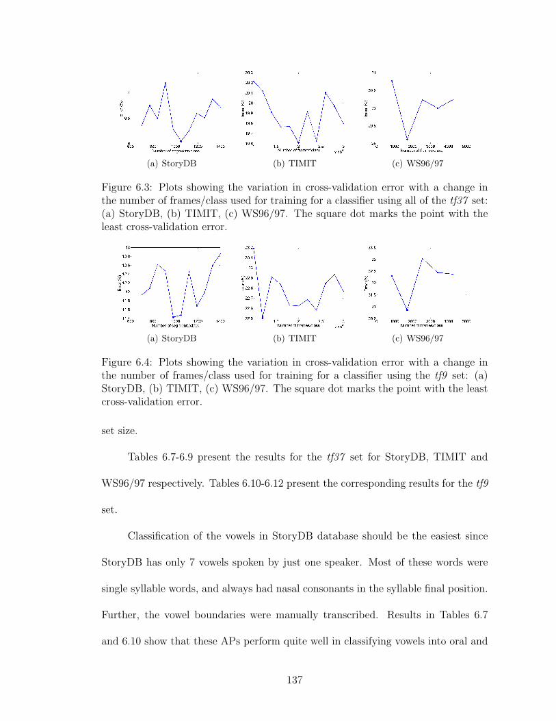
(a) StoryDB (b) TIMIT (c) WS96/97

Figure 6.3: Plots showing the variation in cross-validation error with a change inthe number of frames/class used for training for a classifier using all of the tf37 set:(a) StoryDB, (b) TIMIT, (c) WS96/97. The square dot marks the point with theleast cross-validation error.

(a) StoryDB (b) TIMIT (c) WS96/97

Figure 6.4: Plots showing the variation in cross-validation error with a change inthe number of frames/class used for training for a classifier using the tf9 set: (a)StoryDB, (b) TIMIT, (c) WS96/97. The square dot marks the point with the leastcross-validation error.

set size.

Tables 6.7-6.9 present the results for the tf37 set for StoryDB, TIMIT and

WS96/97 respectively. Tables 6.10-6.12 present the corresponding results for the tf9

set.

Classification of the vowels in StoryDB database should be the easiest since

StoryDB has only 7 vowels spoken by just one speaker. Most of these words were

single syllable words, and always had nasal consonants in the syllable final position.

Further, the vowel boundaries were manually transcribed. Results in Tables 6.7

and 6.10 show that these APs perform quite well in classifying vowels into oral and

137

Table 6.7: Classification results for oral vs nasalized vowels using the tf37 set.Training database: StoryDB, Testing database: StoryDB.

% Correct (Linear) % Correct (RBF) Test Tokens

Oral Vowels 95.54 97.32 112

Nasalized Vowels 89.88 97.02 336

Chance Norm. Acc. 92.71 97.17 448

Table 6.8: Classification results for oral vs nasalized vowels using the tf37 set.Training database: TIMIT, Testing database: TIMIT.

% Correct (Linear) % Correct (RBF) Test Tokens

Oral Vowels 81.06 87.64 14136

Nasalized Vowels 72.11 75.53 4062

Chance Norm. Acc. 76.58 81.59 18198

Table 6.9: Classification results for oral vs nasalized vowels using the tf37 set.Training database: WS96/97, Testing database: WS96/97.

% Correct (Linear) % Correct (RBF) Test Tokens

Oral Vowels 70.90 74.44 12373

Nasalized Vowels 68.01 70.87 1119

Chance Norm. Acc. 69.45 72.65 13492

138

nasalized categories in this simple task. Chance normalized accuracies for the tf37

set with the RBF SVM classifier decrease progressively from 97.17% for StoryDB

to 81.59% for TIMIT to 72.65% for WS96/97 as the classifier is presented with

increasingly complicated tasks. Corresponding accuracies for the tf9 set fall from

96.28% for StoryDB to 77.90% for TIMIT to 69.58% for WS96/97. Thus, there is

about a 3% reduction in chance normalized accuracy as the set of APs is changed

from the tf37 set to the tf9 set. This shows that the selected set of 9 APs is not

capturing all the information. However, the 3% reduction should be acceptable

given the large reduction in the number of APs from 37 to 9. Tables 6.7-6.12 also

show that the results using the knowledge-based APs proposed in this study are

much more balanced across the oral and nasalized vowel classes when compared to

the results for MFCCs.

Table 6.10: Classification results for oral vs nasalized vowels using the tf9 set.Training database: StoryDB, Testing database: StoryDB.

% Correct (Linear) % Correct (RBF) Test Tokens

Oral Vowels 83.93 95.54 112

Nasalized Vowels 96.13 97.02 336

Chance Norm. Acc. 90.03 96.28 448

6.3 Comparison between current and baseline results

Figures 6.5a and 6.5b plot histograms showing a comparison between the dif-

ferent sets of APs for StoryDB, TIMIT and WS96/97 with Linear and RBF SVM

139

(a) Linear Kernel

(b) RBF Kernel

Figure 6.5: Histograms showing a comparison between the results obtained withseveral different sets of APs: (a) Results with Linear SVM Classifiers, (b) Resultswith RBF SVM Classifiers.

140

Table 6.11: Classification results for oral vs nasalized vowels using the tf9 set.Training database: TIMIT, Testing database: TIMIT.

% Correct (Linear) % Correct (RBF) Test Tokens

Oral Vowels 75.75 81.18 14136

Nasalized Vowels 71.42 74.62 4062

Chance Norm. Acc. 73.58 77.90 18198

Table 6.12: Classification results for oral vs nasalized vowels using the tf9 set.Training database: WS96/97, Testing database: WS96/97.

% Correct (Linear) % Correct (RBF) Test Tokens

Oral Vowels 68.27 73.56 12373

Nasalized Vowels 66.85 65.59 1119

Chance Norm. Acc. 67.56 69.58 13492

classifiers, respectively. Note that in these figures, the bars for the gs6 set are

missing for StoryDB because, as mentioned earlier in Section 6.1.1, StoryDB did

not have an adequate number of oral vowel segments for proper training. Hence,

StoryDB was not used with the gs6 set. It is clear from these figures that:

1. The overall performance of the tf37 set is the best in all the cases.

2. The performance of the gs6 set is the worst in all the cases where it was

tested except when Linear SVM classifiers were used for TIMIT where it out-

performed the mf39 set.

3. The performance of the mf39 set improves significantly with RBF SVM clas-

sifiers. However, even with the RBF SVM classifiers, the performance of this

141

set is not very good for the spontaneous speech database WS96/97.

4. The difference in the performance of the tf37 set and the tf9 is not very large

for any of the cases.

5. The performance of the tf37 and tf9 sets is very balanced across the oral

and nasalized vowel classes, especially so for linear classifiers. On the other

hand, the performance of the gs6 and mf39 sets differs widely across the oral

and nasalized vowel classes. For example, for the gs6 set there is a difference

of about 12% in the accuracies for oral and nasalized vowels for the TIMIT

database with a linear SVM classifier. The differences are much more signif-

icant for the mf39 set. In fact, the accuracy of the mf39 set for nasalized

vowels is even below the chance accuracy of 50% for three cases (for TIMIT

and WS96/97 with linear classifiers, and for WS96/97 with RBF classifier).

Figure 6.6 plots a histogram showing a comparison between the frame based

results obtained in WS04 JHU Workshop (Hasegawa-Johnson et al., 2004, 2005) and

the frame based results obtained in this study using the tf9 set. These results are

for the test set of WS96/97 database which was obtained by alternating the files in

both cases. Both sets of results were obtained by using a Linear SVM Classifier.

The figure shows that the results using the tf9 set are better than the ws04 results

for vowels /aa/, /ah/, /ax/, /ay/, /eh/, /ih/ and /ow/. Further, note that the

variation in the results across vowels is much smaller when using the tf9 set. That

is, the results using the tf9 are more vowel independent as compared to the ws04

results. It must also be noted that the total number of test tokens used to get the

142

Figure 6.6: Histogram showing a comparison between the frame based results ob-tained in JHU WS04 Workshop (Hasegawa-Johnson et al., 2004, 2005) and the framebased results obtained in this study using the tf9 set.

143

results for the tf9 set was 180347, which is much larger than the 18012 test tokens

used to get the ws04 results.

6.4 Vowel Independence

Table 6.13: Results for each vowel for StoryDB using the tf9 set with an RBF SVM.

Oral Vowels Nasalized Vowels Oral + Nasalized Vowels

Vowel % Correct Tokens % Correct Tokens Chance Norm. Tokens

aa 100.00 16 91.67 48 95.83 64

ae 100.00 16 100.00 48 100.00 64

ah 93.75 16 89.58 48 91.67 64

eh 100.00 16 100.00 48 100.00 64

ih 75.00 16 100.00 48 87.50 64

iy 100.00 16 100.00 48 100.00 64

uw 100.00 16 97.92 48 98.96 64

Tables 6.13-6.15 show the breakup of the overall results into the results for

individual oral vowels, nasalized vowels, and chance normalized accuracies/vowel

using the tf9 set with an RBF SVM classifier. Figures 6.7a and 6.7b plot these

results for TIMIT and WS96/97. These tables and figures help in understanding

the dependence of the results on vowel context. Note that, in Tables 6.14 and 6.15

and correspondingly in Figures 6.7a and 6.7b, the scores for syllabic nasals under the

oral vowel category are 0 % because all syllabic nasals were considered as nasalized.

The chance normalized accuracies are very low for the syllabic nasals for this same

144

reason. The results for StoryDB in Table 6.13 are not very interesting because the

number of vowel segments is very small, and the accuracies are very high for all the

vowels. The results for TIMIT and WS96/97 give much more insight and they will

be described in detail now.

Table 6.14: Results for each vowel for TIMIT using the tf9 set with an RBF SVM.

Oral Vowels Nasalized Vowels Oral + Nasalized Vowels

Vowel % Correct Tokens % Correct Tokens Chance Norm. Tokens

iy 93.17 1946 62.39 218 77.78 2164

ih 89.71 1098 75.96 416 82.84 1514

eh 78.68 1018 72.52 302 75.60 1320

ey 87.99 533 80.65 155 84.32 688

ae 74.87 975 87.60 250 81.24 1225

aa 82.74 869 75.74 136 79.24 1005

aw 74.50 149 82.69 52 78.59 201

ay 75.74 643 79.35 92 77.54 735

ah 73.72 449 74.10 332 73.91 781

ao 79.54 904 72.73 99 76.13 1003

oy 68.79 141 93.94 33 81.37 174

ow 74.01 404 74.07 270 74.04 674

uh 86.29 197 56.25 16 71.27 213

Continued on next page

145

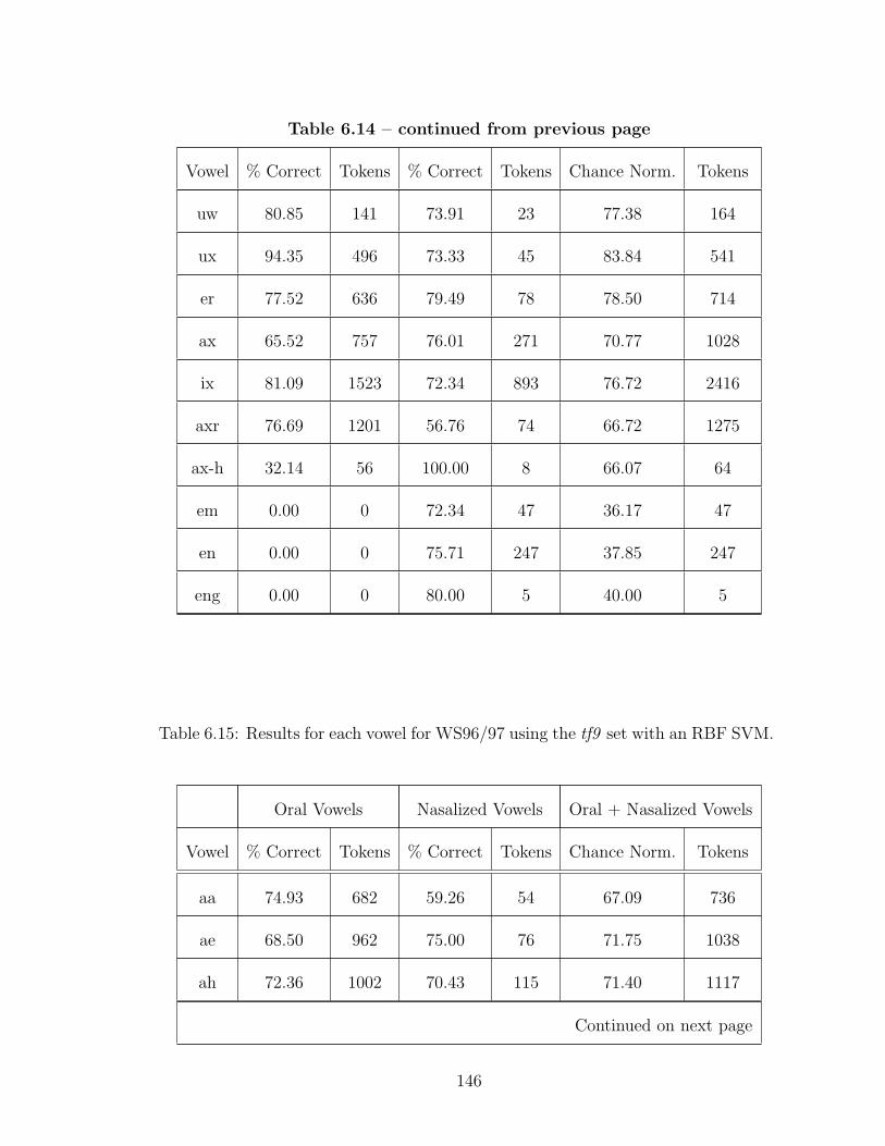
Table 6.14 – continued from previous page

Vowel % Correct Tokens % Correct Tokens Chance Norm. Tokens

uw 80.85 141 73.91 23 77.38 164

ux 94.35 496 73.33 45 83.84 541

er 77.52 636 79.49 78 78.50 714

ax 65.52 757 76.01 271 70.77 1028

ix 81.09 1523 72.34 893 76.72 2416

axr 76.69 1201 56.76 74 66.72 1275

ax-h 32.14 56 100.00 8 66.07 64

em 0.00 0 72.34 47 36.17 47

en 0.00 0 75.71 247 37.85 247

eng 0.00 0 80.00 5 40.00 5

Table 6.15: Results for each vowel for WS96/97 using the tf9 set with an RBF SVM.

Oral Vowels Nasalized Vowels Oral + Nasalized Vowels

Vowel % Correct Tokens % Correct Tokens Chance Norm. Tokens

aa 74.93 682 59.26 54 67.09 736

ae 68.50 962 75.00 76 71.75 1038

ah 72.36 1002 70.43 115 71.40 1117

Continued on next page

146

Table 6.15 – continued from previous page

Vowel % Correct Tokens % Correct Tokens Chance Norm. Tokens

ao 65.79 380 62.50 24 64.14 404

aw 70.25 158 73.68 19 71.97 177

ax 60.69 1038 60.00 35 60.35 1073

ay 73.26 875 66.67 21 69.96 896

eh 73.60 1144 69.07 97 71.34 1241

ey 78.98 647 56.25 16 67.61 663

ih 78.10 1726 68.11 185 73.10 1911

ix 73.75 579 73.81 42 73.78 621

iy 82.92 1464 66.67 69 74.80 1533

ow 59.04 581 73.26 86 66.15 667

oy 67.74 31 50.00 4 58.87 35

uh 75.58 471 100.00 5 87.79 476

uw 79.92 473 25.00 4 52.46 477

ux 84.38 160 0.00 0 42.19 160

em 0.00 0 54.39 57 27.19 57

en 0.00 0 56.86 204 28.43 204

eng 0.00 0 50.00 6 25.00 6

Tables 6.14 and 6.15 and Figure 6.7 show that there are clearly individual

147

(a) TIMIT

(b) WS96/97

Figure 6.7: Histograms showing the results for each vowel for (a) TIMIT and (b)WS96/97, using the tf9 set with an RBF SVM Classifier.

148

differences in vowel accuracies. Note that the results for vowels /uh/, /ax-h/ and

/eng/ for TIMIT, and vowels /oy/, /uh/, /uw/, /ux/ and /eng/ for WS96/97 should

be treated with caution since there were very few test tokens for the nasalized

segments for these vowels. Further, note that these are also the vowels for which

very few training tokens were available. Thus, it is very likely that the results for

these vowels would improve significantly if more training data for these vowels was

provided.

It can be seen from the tables, that if the results for these vowels along with the

syllabic nasals are disregarded, then the overall chance normalized accuracies/vowel

are more or less independent of the vowel context. A glance at Figure 6.7 suggests

that even though the chance normalized accuracies for different vowels appear to

be constant, the individual vowel differences are much more prounounced for the

two categories of oral and nasalized vowels. This result suggests that there is a

somewhat inverse relationship between the scores for oral and nasalized classes for

several vowels, i.e., if the score for the oral class is above average for a particular

vowel, then the score for the nasalized class for that vowels is below average, and vice

versa. High vowels like /iy/ and /uw/ are more biased towards correctly recognizing

oral vowels, whereas low vowels like /aa/ and /ae/ are biased more towards correctly

recognizing nasalized vowels. This rule for low and high vowels does not seem to hold

very well for the results for WS96/97. But this could also be happening because

a much higher number of training tokens were used for TIMIT as compared to

WS96/97. Thus, it is possible that the results for WS96/97 would conform more

strongly with the results for TIMIT if more training tokens were available. Also

149

note that the results are not dependent on the vowel stress level since the accuracies

for reduced vowels (/ax/, /axr/, /ax-h/, /ix/ and /ux/) are not too low.

6.5 Category and Language Independence

Table 6.16: Classification results for oral vs nasalized vowels using the tf37 set.Training database: WS96/97, Testing database: OGI. Co = Coarticulatorily, Ph =Phonemically.

% Correct (Linear) % Correct (RBF) Test Tokens

Oral Vowels 66.79 77.95 6989

All Nasalized Vowels 60.59 46.77 1454

Co Nasalized Vowels 57.58 43.76 1266

Ph Nasalized Vowels 80.85 67.02 188

Chance Norm. Acc. 63.69 62.36 8443

Table 6.17: Classification results for oral vs nasalized vowels using the tf9 set.Training database: WS96/97, Testing database: OGI. Co = Coarticulatorily, Ph =Phonemically.

% Correct (Linear) % Correct (RBF) Test Tokens

Oral Vowels 71.38 74.60 6989

All Nasalized Vowels 56.05 50.21 1454

Co Nasalized Vowels 53.48 47.95 1266

Ph Nasalized Vowels 73.40 65.43 188

Chance Norm. Acc. 63.72 62.40 8443

In this experiment, the classifier trained for the telephone speech database

150

Table 6.18: Classification results for oral vs nasalized vowels using the mf39 set.

Training database: WS96/97, Testing database: OGI. Co = Coarticulatorily, Ph =

Phonemically.

% Correct (Linear) % Correct (RBF) Test Tokens

Oral Vowels 88.90 85.02 6989

All Nasalized Vowels 19.33 37.35 1454

Co Nasalized Vowels 16.03 34.52 1266

Ph Nasalized Vowels 41.49 56.38 188

Chance Norm. Acc. 54.11 61.18 8443

WS96/97 was used to test oral and nasalized vowel tokens extracted from the OGI

telephone speech database for Hindi language without retraining of any kind. The

goal of this experiment was to evaluate the performance of the proposed APs on

identifying nasalization in vowels which had not yet been seen by the classifier, and

to test the performance of this classifier on phonemically nasalized vowels.

Tables 6.16-6.19 show the results for this task using the tf37, tf9, mf39 and

gs6 sets, respectively, with Linear and RBF SVM classifiers. Results suggest that

for all the parameter sets except the mf39 set, Linear classifiers give better overall

performance. Further, the accuracies obtained by using the RBF SVM classifiers

are very unbalanced (the accuracies for nasalized vowels are very low). In fact,

the accuracies for nasalized vowels were extremely poor with the mf39 set. The

overall performance of the gs6 set was close to the performance with the tf37 and

tf9 sets. Note, however, that the gs6 set had segment-based APs not frame-based.

151

Table 6.19: Classification results for oral vs nasalized vowels using the gs6 set.

Training database: WS96/97, Testing database: OGI. Co = Coarticulatorily, Ph =

Phonemically.

% Correct (Linear) % Correct (RBF) Test Tokens

Oral Vowels 60.17 59.35 6989

All Nasalized Vowels 65.27 63.41 1454

Co Nasalized Vowels 64.38 63.19 1266

Ph Nasalized Vowels 71.28 64.89 188

Chance Norm. Acc. 62.72 61.38 8443

Best overall performance on this cross-language task was obtained by using the tf9

set. The chance normalized accuracy of 63.72% with the tf9 set suggests at least

some amount of language independence. This result is very encouraging since this

test was performed without any retraining of the classifier trained for the WS96/97

English database. The results would most likely increase if the classifier was first

trained on samples of Hindi. However, even the fact that these same APs can be

used for another language is very encouraging since it suggests that we are capturing

the relevant information.

Further, note that the accuracy for phonemically nasalized vowels is much

higher than that for coarticulatorily nasalized vowels for all the parameter sets (for

example, 80.85% vs 57.58% for tf37 set, and 73.40% vs 53.48% for tf9 set). This

suggests that

1. The same APs which are used to capture coarticulatory nasalization can be

152

used to capture phonemic nasalization. This result is in line with the view

expressed by Dickson (1962) where it was suggested that the acoustic cues are

the same irrespective of the category of nasality.

2. The acoustic characteristics of nasalization are much more strongly expressed

(both in degree and duration) when vowels are phonemically nasalized. How-

ever, the better accuracies for coarticulatorily nasalized vowels with the gs6

set (which is a set of segment-based APs) arouses the suspicion that the clas-

sification procedure used (see Section 3.3.5) may be the major reason for the

lower accuracies for coarticulatorily nasalized vowels with the other sets of

APs. To confirm this suspicion, another experiment was performed in which

instead of using all the frames in a segment (as suggested in 3.3.5), only the

last 1/3rd of the frames in a vowel segment were used to decide whether a

vowel was nasalized or not. Results of this experiment showed that the scores

for coarticulatorily nasalized vowels did indeed increase by about 4-5% while

the results for phonemically nasalized vowels did not change significantly, thus

confirming the suspicion that the smaller duration of nasalization in coarticu-

latorily nasalized vowels may be the main reason for lower accuracies. In this

experiment, however, the accuracies for oral vowels also reduced by almost an

equal amount for all the databases. That is, with this classification strategy,

the classifier gets biased towards correctly recognizing nasalized vowels. Thus,

it is debatable what the best scoring strategy may be. Further, a classifier

using this scoring strategy would not be able to classify vowels preceeded by

153

(a) TIMIT (b) WS96/97

Figure 6.8: PDFs of the duration of correct and erroneous oral and nasalized vowelsfor (a) TIMIT, (b) WS96/97.

nasal consonants as nasalized at all.

It must be noted, however, that the number of test tokens for phonemically nasalized

vowels was not very high. Thus, the result would become much more reliable if it

could be tested on a larger set of phonemically nasalized vowels.

6.6 Error Analysis

This section presents a detailed analysis of the errors made by the algorithm

to understand the sources of error and suggest possible improvements. All of the

figures presented in this section are based on the results of the RBF SVM classifier

using the tf9 set.

6.6.1 Dependence on Duration

Figures 6.8a and 6.8b show PDFs of the duration of correct and erroneous

segments of oral and nasalized vowels for TIMIT and WS96/97 respectively. A look

154

Figure 6.9: Histograms showing the dependence of the Errors in the classificationof Oral and Nasalized Vowels in TIMIT database on the speaker’s gender.

at these PDFs suggests that there is hardly any difference between the durations of

either oral and nasalized vowel segments, or correct and erroneous vowel segments.

This result should be expected because duration has not been incorporated into the

classifier in any way. However, this is contrary to the results of human perceptual

studies (cf. Delattre and Monnot (1968); Whalen and Beddor (1989)) where it

was shown that French and American English listeners judged vowels with longer

duration as more nasal.

155

6.6.2 Dependence on Speaker’s Gender

Figure 6.9 plots the histograms for the % of Errors per gender category (=

(Number of Erroneous segments for the category/Total number of segments for that

category)*100 ) for TIMIT. The Number of Erroneous Segments/Total number of

Segments is also displayed on the top of each bar. The histograms clearly show that

the % of Errors is much higher for females. This is in agreement with the results

for males and females obtained by Glass (1984). The histograms also suggest that

the classifier is biased towards classifying vowel segments for females as nasalized,

thus leading to a lower % of error for the nasalized vowel segments for females. On

the other hand, for males the classifier is biased towards calling all vowels as oral.

The results obtained by Glass (1984) did not display this relationship, although it

must be noted that in the study by Glass, the database only consisted of 6 speakers

(3 male and 3 female). To my knowledge, there have been no perceptual studies

which suggest that listeners find it more difficult to classify vowels produced by

females into oral and nasalized classes, or which suggest that the vowels produced

by females are more frequently classified as nasalized as compared to the vowels

produced by males. However, Klatt and Klatt (1990) did suggest that the speech

of females is more breathy, and breathiness was shown to possess several qualities

similar to nasalization.

156

(a) Number of Errors

(b) % of Errors

Figure 6.10: Dependence of errors in the classification of oral vowels on the rightcontext for TIMIT database: (a) Number of Errors, (b) % of Errors.

157

(a) Number of Errors

(b) % of Errors

Figure 6.11: Dependence of errors in the classification of oral vowels on the rightcontext for WS96/97 database: (a) Number of Errors, (b) % of Errors.

158

6.6.3 Dependence on context

Figures 6.10 and 6.11 plot histograms showing the number and percentage of

errors in the classification of oral vowels for different right contexts for TIMIT and

WS96/97, respectively. Contexts for which the count of oral vowels was less than 50

were not plotted since the results would not be very reliable for such small counts.

Figures 6.10a and 6.11a show that most of the errors for oral vowels occur when

vowels are in the context of consonants (stops, fricatives, semivowels), aspirated

sounds (/hh/ or /hv/), or when they occur at the end of the utterance (context

/h#/). Very few errors occur when vowels are in the context of other vowels.

Figures 6.10 and 6.11 also show that the number of errors varies widely with

context. However, the variation across context is much less prominent in Figures

6.10b and 6.11b which plot the % of Errors for each right context. This suggests that

for most of the contexts, more errors occur for a particular right context only because

the total number of vowels occurring in that particular context is high. However,

one context that clearly stands out in both Figure 6.10b and 6.11b is /h#/. This

is possible because vowels are frequently breathy at the end of the utterance, and

breathiness has been shown to possess many cues similar to nasalization (Klatt and

Klatt, 1990).

6.6.4 Syllable initial and syllable final nasals

As described in Section 3.1.2, all vowels followed by nasal consonants were

assumed to be nasalized for TIMIT. However, this can be a potential source of

159

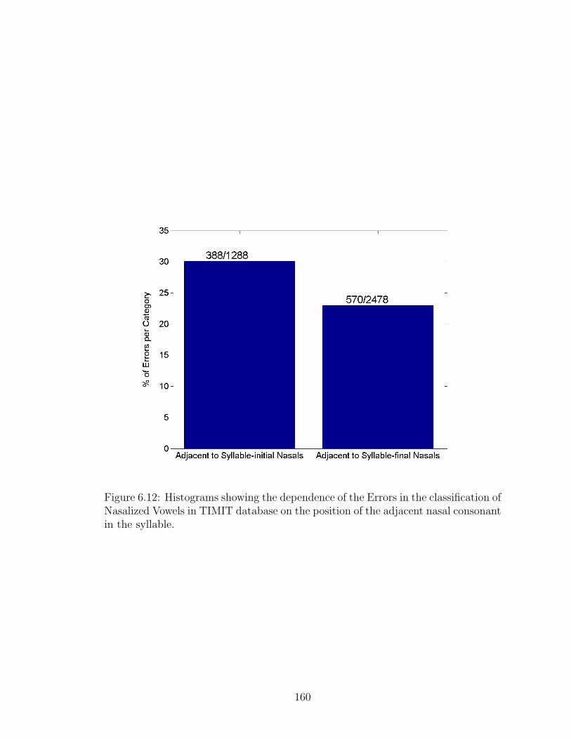
Figure 6.12: Histograms showing the dependence of the Errors in the classification ofNasalized Vowels in TIMIT database on the position of the adjacent nasal consonantin the syllable.

160

error, since vowels would most likely get nasalized only when they are followed by a

nasal consonant in syllable-final position. Therefore, it may be worthwhile to find

out it was actually a source of error. Even though syllable boundaries were not

marked for TIMIT, the following simple rules proposed by Kahn (1976) were used

to divide all the nasalized vowels considered into those adjacent to syllable-final

nasal consonants, and those adjacent to syllable-initial nasal consonants:

1. If the context surrounding a nasal consonant is VNC, then the nasal is always

in the syllable-final position.

2. If the context surrounding a nasal consonants is VNV, then the nasal consoant

is in the syllable-initial position.

Figure 6.12 shows the histogram of the % of Errors in the classification of

nasalized vowels in TIMIT database divided into the two categories: vowels adja-

cent to syllable-final nasal consonants, and vowels adjacent to syllable-initial nasal

consonants. The numbers over the bars give the Number of Erroneously classified

nasalized vowels in a category/Total number of nasalized vowels in that category.

Results show that the % of Errors is higher for vowels preceding syllable-initial

nasal consonants, which supports the view that vowels before syllable-initial nasal

consonants are not very strongly nasalized.

6.7 Chapter Summary

Results for the knowledge-based APs proposed in this study were presented

in this chapter. These results were also compared with several sets of baseline

161

results. Chance normalized accuracies of 96.28%, 77.90% and 69.58% were obtained

for StoryDB, TIMIT and WS96/97 respectively by using the 9 best APs selected in

Chapter 5 in an RBF SVM classifier framework. The performance of these APs was

much better than the baseline results. Further, the classifier was found to perform

well for all vowels, thus showing some amount of vowel independence. These APs

were also tested on a database of Hindi without any retraining of the classifier

trained for the WS96/97 English database. Chance normalized accuracy of 63.72%

with a Linear SVM classifier on this cross-language task suggests some amount of

language independence. Further, the accuracy for phonemically nasalized vowels was

found to be much higher than that for coarticulatorily nasalized vowels. Analysis

suggested that the main reason for the higher accuracy for phonemically nasalized

vowels may be that the duration of nasalization is much longer for phonemically

nasalized vowels.

162

Chapter 7

Summary, Discussion and Future Work

7.1 Summary

The goals of this thesis were twofold: (1) To understand the acoustic charac-

teristics of vowel nasalization and the sources of acoustic variability in the spectra of

nasalized vowels through spectral analysis and vocal tract modeling, and (2) To de-

velop Acoustic Parameters (APs) based on the knowledge gained though the spectral

analysis and vocal tract modeling for the automatic detection of vowel nasalization.

The vocal tract modeling study presented in Chapter 4 has improved upon

the existing knowledge base on nasalization, and provided critical insights into the

acoustic characteristics of nasalization. Analysis of the simulated spectra has shown

that the spectrum of nasalized vowels is extremely complicated because of a multi-

tude of extra poles and zeros introduced into the spectrum because of velar coupling,

asymmetry of the nasal passages, and the sinuses. It was shown that the asymmetry

between the nasal passages introduces extra pole-zero pairs in the spectrum due to

the branching effect. Simulations with the inclusion of maxillary and sphenoidal

sinuses showed that each sinus can potentially introduce one extra pole-zero pair in

the spectrum (maxillary sinuses produced the poles lowest in frequency). Further,

it was suggested that most of these poles at higher frequencies may just appear

as ripples when losses are added. The main spectral changes were found to occur

163

because of the poles due to the nasal coupling and the maxillary sinus.

A detailed analysis of the poles and zeros due to the sinuses suggested that the

effective frequencies of the poles and zeros due to the sinuses in the combined output

of the oral and nasal cavities change with a change in the oral cavity configuration

for nasalized vowels. This change in the oral cavity configuration may be due to

a change in the coupling area, or due to a change in the vowel being articulated.

Thus, it was predicted that nasalized vowel regions may not be very useful for the

purposes of speaker recognition since the acoustic characteristics of the fixed sinus

cavities in the nasalized vowel spectrum can change even when there is no change

in the configuration of the sinus cavities. At the same time, it was also predicted

that the frequencies of the zeros due to the sinuses will not change in the spectra of

nasal consonants, thus supporting the use of nasal consonantal regions for speaker

recognition. This study has also helped us in clearly understanding the reasons

behind all the acoustic correlates of vowel nasalization which have been proposed in

past literature.

Based on a detailed survey of the past literature and the knowledge gained

from the vocal tract modeling study, 37 APs were proposed for the automatic de-

tection of vowel nasalization. Out of this set of 37 APs, 9 APs with the best dis-

crimination capability were selected for the task of classifying vowel segments into

oral and nasalized categories. These APs were tested in a Support Vector Machine

(SVM) classifier framework on three different databases with different sampling

rates, recording conditions, and a large number of male and female speakers. Accu-

racies of 96.28%, 77.90% and 69.58% were obtained by using these APs on StoryDB,

164

TIMIT and WS96/97, respectively with a Radial Basis Function (RBF) kernel SVM.

These results were compared with baseline results obtained by using two different

sets of APs in the current experimental framework. The results were also compared

with the results obtained during the WS04 JHU workshop. Comparison with the

baseline results showed that the APs proposed in this study not only formed the

most compact set (9 APs as opposed to 39 MFCCs, and approximately 400 APs

used in the WS04 JHU workshop), but also gave the best performance on this task.

The performance of the classifier trained using the proposed APs on WS96/97

English database was also tested on a database of Hindi without retraining of any

kind. Chance normalized accuracy of 63.72% was obtained on this task. This is

very encouraging given that the classifier was not trained on any samples from

Hindi at all. Testing on this database of Hindi also lends the opportunity to test the

performance of these APs on phonemically nasalized vowels which are an integral

part of Hindi, and were actually transcribed in this particular database. An accuracy

of 73.40% was obtained for the phonemically nasalized vowels, which was much

higher than the accuracy of 53.48% for coarticulatorily nasalized vowels. The results

of this experiment are particularly interesting because this suggests that (1) we are

really getting at the right information, (2) the same APs can be used to capture

nasalization in different languages, and (3) the same APs can be used to capture both

coarticulatory nasalization and phonemic nasalization. Further, the better accuracy

for phonemically nasalized vowels suggests that the duration of nasalization is much

longer when vowels are phonemically nasalized.

165

7.2 Discussion

The qualities of a set of ideal knowledge-based APs which capture a particular

phonetic feature (eg. nasalization) should be:

1. They should reliably capture all of the acoustic characteristics of the feature

they are targeted at.

2. They should only capture the acoustic characteristics of the feature they are

targeted at disregarding all variations due to other factors.

In this case, these rules mean that the proposed APs should capture all of

the acoustic characteristics of nasalization reliably, and they should disregard all

variations due to vowels, speakers and their gender, language and category. In this

thesis, an attempt was made to achieve these goals as best as possible.

Results for the classification of individual vowels into oral and nasal categories

suggested that the proposed APs are independent of the vowel context to a large

extent. However, speaker independence is still a problem, as is clear from the results

for males and females. Different speakers may have a very different configuration

of the nasal cavity. Further, speakers may have their own idiosyncrasies. Some

speakers may nasalize vowels to a much stronger degree than other speakers. Some

speakers may nasalize all vowels even if they are not in the context of a nasal con-

sonant, maybe because of anatomical defects or nervous system damage, or maybe

even otherwise. Thus, values of the APs for the oral vowel of one speaker may

overlap with the values of the APs for nasalized vowels of another speaker. In fact,

speaker variation is one of the major reasons for the difficulty in classifying vowels

166

into oral and nasal categories (as is clear from the results for StoryDB which only

had one speaker). Thus, more work is needed to counter the variation due to speak-

ers. Results from the experiment on Hindi are proof to the language and category

independence of the proposed APs. However, any system with incomplete knowl-

edge needs statistical methods to counter the variation due to ignorance. Thus, the

accuracy would surely increase with retraining of the classifier on Hindi. But even

the fact that the same APs can be used is very encouraging since it suggests that

we are moving in the right direction.

7.3 Future Work

There are many directions in which this research can be extended. Some of

the possible ideas are discussed in this section.

1. Vocal tract modeling: Even though the vocal tract modeling study pre-

sented in this thesis has given a quantum improvement in the understanding

of nasalization, it has still left some of the questions unanswered. The area

function data used in this study did not include the Ethmoidal and Frontal

sinuses. Thus, a more detailed data which includes these sinuses is required to

understand the acoustic effects of these sinuses. The available vocal tract area

functions were recorded during the production of oral vowels. Recording the

area functions during the production of nasalized vowels possibly with varying

coupling areas would be very useful for a much more accurate modeling of

the acoustic characteristics of nasalization. Further, the available data was

167

recorded for only one speaker. Recordings of the vocal tract and nasal tract

area functions for a number of speakers would be very useful in understanding

speaker variability.

2. Improvements to the pattern recognition approach: The performance

of any automatic classification system depends to a large extent on the pat-

tern recognition methodology used including the training data, the training

procedure, the classification procedure, and the pattern recognizer itself. The

goal of this thesis was to develop acoustic parameters to automatically classify

oral and nasalized vowels. Hence, this thesis did not focus on finding the best

pattern matching approach although a reasonable effort was spent to optimize

the training procedure and the classification procedure. Thus, improvements

to the results may be possible by using a different pattern recognizer like a

Hidden Markov Model (HMM) which may be able to model the dynamic infor-

mation in a better manner. Another possibility is to use acoustic parameters

extracted from not only the current frame, but also from a number of frames

before and after the current frame to decide whether the current frame is

nasalized or not. Further, as discussed in Section 6.5, it may also be possible

to improve the classification procedure.

3. Performance in noise: The performance of these APs should be tested

in the presence of noise. Even if the performance of these APs is not very

good in noise, it is our belief that an approach based on the extraction of

these APs from an enhanced version of the speech signal should lead to more

168

robust performance. A speech enhancement scheme called the Modified Phase

Opponency (MPO) model has been proposed by Deshmukh (2006). Thus, it

may be worthwhile to explore the performance of these APs in noise using the

MPO-enhanced speech signal.

4. Incorporation into a Landmark-based Speech Recognition System:

The proposed knowledge-based APs should be incorporated into the landmark-

based speech recognition system developed in our lab (Juneja, 2004). This

would enable this system to classify vowels into oral and nasalized classes, and

hence, complete another classification node in the phonetic feature hierarchy

shown in Figure 1.2. A pronunciation model based on phonetic features can use

this information to learn that a nasalized vowel is a high probability substitute

for a nasal consonant. Also, as described earlier, inclusion of nasalization into

this system would make it much more useful for languages with phonemic

nasalization.

5. Hypernasality detection: These APs should be tested on the task of detect-

ing hypernasality in a non-intrusive manner. Since the proposed APs would

work only in the vowel regions, the first pass of such a system for hypernasality

detection has to be a broad classifier which segments the vowel regions in the

input speech. These APs can then be used in the vowel regions to obtain a

nasality score for each vowel segment which can be averaged to obtain a score

for the speaker. A database with hypernasality judgments made by other

means would be required to test the performance of this system. Average

169

nasality score for a speaker obtained by the procedure described above should

also be useful as a parameter for speaker recognition.

170

Appendix A

TIMIT and IPA Labels

TIMIT IPA Example TIMIT IPA Example Vowel Properties

p p pea iy i beet high front tense

b b bee ih I bit high front lax

t t tea eh E bet middle front lax

d d day ey e bait middle front tense

k k key ae æ bat low front lax

g g gay aa A bott low back lax

dx R muddy aw aU bout low central lax

q P bat ay aI bite low central tense dip

jh à joke ah 2 but

ch Ù choke ao O bought middle back lax rnd

f f fin oy OI boy middle back tense rnd dip

v v van ow o boat middle back tense rnd

th T thin uh U book high back lax rnd

dh D then uw u boot high back tense rnd

s s sea ux u toot

z z zone er Ç bird high central lax rcld (str)

sh S she ax @ about middle central lax (unstr)

171

zh Z azure ix |I debit

m m mom axr Ä butter high central lax rcld (unstr)

n n noon ax-h @h suspect

ng N sing

em m"

bottom

en n"

button

eng N"

washington

nx R winner

l l lay

r r ray

w w way

y j yacht

hh h hay

hv H ahead

el l"

bottle

rnd: rounded, rcld: r-colored, str: stressed, unstr: unstressed, dip: diphthong

172

Appendix B

Vocal Tract Modeling Simulations

Vocal tract simulations for the vowels /ae/, /ah/, /eh/, /ih/ and /uw/ are

shown in this appendix. These figures directly correspond with the analysis that

was presented in Chapter 4 for the vowels /aa/ and /iy/.

Figure B.1: Areas for the oral cavity for the vowels /ae/, /ah/, /eh/, /ih/ and /uw/

173

(a) Transfer Functions for /ae/ (b) Transfer Functions for /ae/

(c) Susceptance plots for /ae/ (d) Susceptance plot for /ae/, Coupling =0.4cm2

Figure B.2: Plots of the transfer functions and susceptances for /ae/. (a) Transferfunctions for different coupling areas, (b) Transfer functions for a particular couplingarea but with complexity due to two nostrils and sinuses gradually added, (c) Plots ofsusceptances −(Bp+Bo) and Bn for different coupling areas, (d) Plot of susceptances−(Bp + Bo) (dashed blue) with Bn (solid red) when all the sinuses are included.

174

(a) Spectrogram of cat (b) Spectrogram of cant

(c) Non-nasalized /ae/ (d) Nasalized /ae/

Figure B.3: Comparison of oral and nasalized vowels and their real and simulatedacoustic spectra. (a) Spectrogram of the word cat. (b) Spectrogram of the wordcant. (c) A frame of spectrum taken at 0.12 s (in solid blue), F1 = 591 Hz, F2 =1898 Hz, F3 = 2428 Hz, F4 = 2938Hz, F5 = 3591 Hz, Frequency of extra peak =245 Hz; Simulated spectrum for non-nasalized /ae/ with losses (in dashed black).(d) A frame of spectrum taken at 0.32 s (in solid blue), F1 = 551 Hz, F2 = 1836 Hz,F4 = 3816 Hz, Frequency of extra peak = 225 Hz; Simulated spectrum for nasalized/ae/ with losses (in dashed black). Simulated spectra generated at a coupling of 0.4cm2.

175

(a) Spectrogram of cap (b) Spectrogram of camp

(c) Non-nasalized /ae/ (d) Nasalized /ae/

Figure B.4: Comparison of oral and nasalized vowels and their real and simulatedacoustic spectra. (a) Spectrogram of the word cap. (b) Spectrogram of the wordcamp. (c) A frame of spectrum taken at 0.15 s (in solid blue), F1 = 551 Hz, F2= 2061 Hz, F3 = 2347 Hz, F4 = 2898 Hz, F5 = 3571 Hz, Small extra peak at265 Hz; Simulated spectrum for non-nasalized /ae/ with losses (in dashed black).(d) A frame of spectrum taken at 0.27 s (in solid blue), F1 = 551 Hz, F2 = 1734Hz, F3 = 2714 Hz, F4 = 3816 Hz, Frequencies of extra peaks = 225 Hz and 2163Hz; Simulated spectrum for nasalized /ae/ with losses (in dashed black). Simulatedspectra generated at a coupling of 0.4 cm2.

176

(a) Transfer Functions for /ah/ (b) Transfer Functions for /ah/

(c) Susceptance plots for /ah/ (d) Susceptance plot for /ah/, Coupling =0.1cm2

Figure B.5: Plots of the transfer functions and susceptances for /ah/. (a) Transferfunctions for different coupling areas, (b) Transfer functions for a particular couplingarea but with complexity due to two nostrils and sinuses gradually added, (c) Plots ofsusceptances −(Bp+Bo) and Bn for different coupling areas, (d) Plot of susceptances−(Bp + Bo) (dashed blue) with Bn (solid red) when all the sinuses are included.

177

(a) Spectrogram of hut (b) Spectrogram of hunt

(c) Non-nasalized /ah/ (d) Nasalized /ah/

Figure B.6: Comparison of oral and nasalized vowels and their real and simulatedacoustic spectra. (a) Spectrogram of the word hut. (b) Spectrogram of the wordhunt. (c) A frame of spectrum taken at 0.20s (in solid blue), F1 = 632 Hz, F2 =1204 Hz, F3 = 2816 Hz, F4 = 3510 Hz, F5 = 4245 Hz, Small extra peak at 285Hz; Simulated spectrum for non-nasalized /ah/ with losses (in dashed black). (d)A frame of spectrum taken at 0.18s (in solid blue), F1 = 591 Hz, F2 = 1224 Hz, F3= 2877 Hz, F4 = 3489 Hz, Frequencies of extra peaks = 285 Hz and 2122 Hz (bothpeaks very small); Simulated spectrum for nasalized /ah/ with losses (in dashedblack). Simulated spectra generated at a coupling of 0.1 cm2.

178

(a) Spectrogram of dub (b) Spectrogram of dumb

(c) Non-nasalized /ah/ (d) Nasalized /ah/

Figure B.7: Comparison of oral and nasalized vowels and their real and simulatedacoustic spectra. (a) Spectrogram of the word dub. (b) Spectrogram of the worddumb. (c) A frame of spectrum taken at 0.09s (in solid blue), F1 = 489 Hz, F2= 1673 Hz, F3 = 2776 Hz, F4 = 3734 Hz, Frequency of extra peak = 245 Hz;Simulated spectrum for non-nasalized /ah/ with losses (in dashed black). (d) Aframe of spectrum taken at 0.14s (in solid blue), F1 = 632 Hz, F2 = 1326 Hz,F3 = 2714 Hz, F4 = 3470 Hz, Frequencies of extra peaks = 245 Hz and 2204 Hz;Simulated spectrum for nasalized /ah/ with losses (in dashed black). Simulatedspectra generated at a coupling of 0.1 cm2.

179

(a) Transfer Functions for /eh/ (b) Transfer Functions for /eh/

(c) Susceptance plots for /eh/ (d) Susceptance plot for /eh/, Coupling =0.3cm2

Figure B.8: Plots of the transfer functions and susceptances for /eh/. (a) Transferfunctions for different coupling areas, (b) Transfer functions for a particular couplingarea but with complexity due to two nostrils and sinuses gradually added, (c) Plots ofsusceptances −(Bp+Bo) and Bn for different coupling areas, (d) Plot of susceptances−(Bp + Bo) (dashed blue) with Bn (solid red) when all the sinuses are included.

180

(a) Spectrogram of get (b) Spectrogram of gem

(c) Non-nasalized /eh/ (d) Nasalized /eh/

Figure B.9: Comparison of oral and nasalized vowels and their real and simulatedacoustic spectra. (a) Spectrogram of the word get. (b) Spectrogram of the wordgem. (c) A frame of spectrum taken at 0.11s (in solid blue), F1 = 306 Hz, F2 =2204 Hz, F4 = 3714 Hz; Simulated spectrum for non-nasalized /eh/ with losses (indashed black). (d) A frame of spectrum taken at 0.18s (in solid blue), F1 = 612Hz, F2 = 1857 Hz, F3 = 2612 Hz, F4 = 3489 Hz, Frequency of extra peak = 245Hz; Simulated spectrum for nasalized /eh/ with losses (in dashed black). Simulatedspectra generated at a coupling of 0.3 cm2.

181

(a) Spectrogram of bet (b) Spectrogram of bent

(c) Non-nasalized /eh/ (d) Nasalized /eh/

Figure B.10: Comparison of oral and nasalized vowels and their real and simulatedacoustic spectra. (a) Spectrogram of the word bet. (b) Spectrogram of the wordbent. (c) A frame of spectrum taken at 0.08s (in solid blue), F1 = 591 Hz, F2= 1734 Hz, F3 = 2367 Hz, F4 = 3571 Hz, Frequency of extra peak = 245 Hz;Simulated spectrum for non-nasalized /eh/ with losses (in dashed black). (d) Aframe of spectrum taken at 0.13s (in solid blue), F1 = 510 Hz, F2 = 1795 Hz, F3= 2714 Hz, F4 = 3734 Hz, Frequency of extra peak = 245 Hz (There is somethingelse at 3081 Hz in both spectra); Simulated spectrum for nasalized /eh/ with losses(in dashed black). Simulated spectra generated at a coupling of 0.3 cm2.

182

(a) Transfer Functions for /ih/ (b) Transfer Functions for /ih/

(c) Susceptance plots for /ih/ (d) Susceptance plot for /ih/, Coupling =0.4cm2

Figure B.11: Plots of the transfer functions and susceptances for /ih/. (a) Transferfunctions for different coupling areas, (b) Transfer functions for a particular couplingarea but with complexity due to two nostrils and sinuses gradually added, (c) Plots ofsusceptances −(Bp+Bo) and Bn for different coupling areas, (d) Plot of susceptances−(Bp + Bo) (dashed blue) with Bn (solid red) when all the sinuses are included.

183

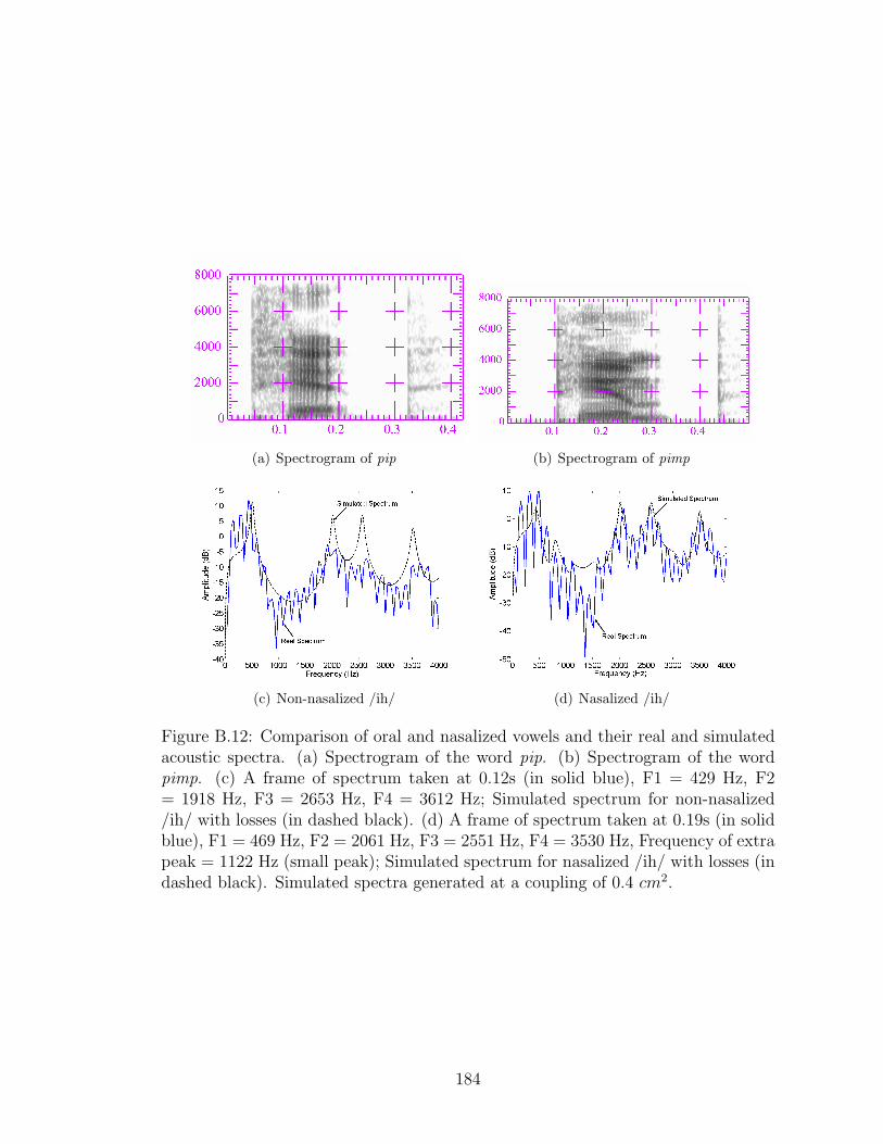
(a) Spectrogram of pip (b) Spectrogram of pimp

(c) Non-nasalized /ih/ (d) Nasalized /ih/

Figure B.12: Comparison of oral and nasalized vowels and their real and simulatedacoustic spectra. (a) Spectrogram of the word pip. (b) Spectrogram of the wordpimp. (c) A frame of spectrum taken at 0.12s (in solid blue), F1 = 429 Hz, F2= 1918 Hz, F3 = 2653 Hz, F4 = 3612 Hz; Simulated spectrum for non-nasalized/ih/ with losses (in dashed black). (d) A frame of spectrum taken at 0.19s (in solidblue), F1 = 469 Hz, F2 = 2061 Hz, F3 = 2551 Hz, F4 = 3530 Hz, Frequency of extrapeak = 1122 Hz (small peak); Simulated spectrum for nasalized /ih/ with losses (indashed black). Simulated spectra generated at a coupling of 0.4 cm2.

184

(a) Spectrogram of hit (b) Spectrogram of hint

(c) Non-nasalized /ih/ (d) Nasalized /ih/

Figure B.13: Comparison of oral and nasalized vowels and their real and simulatedacoustic spectra. (a) Spectrogram of the word hit. (b) Spectrogram of the wordhint. (c) A frame of spectrum taken at 0.10s (in solid blue), F1 = 429 Hz, F2 =2183 Hz, F3 = 2816 Hz, F4 = 3755 Hz; Simulated spectrum for non-nasalized /ih/with losses (in dashed black). (d) A frame of spectrum taken at 0.20s (in solid blue),F1 = 489 Hz, F2 = 2122 Hz, F3 = 2653 Hz, F4 = 3734 Hz, Frequency of extra peak= 1163 Hz (just a bump); Simulated spectrum for nasalized /ih/ with losses (indashed black). Simulated spectra generated at a coupling of 0.4 cm2.

185

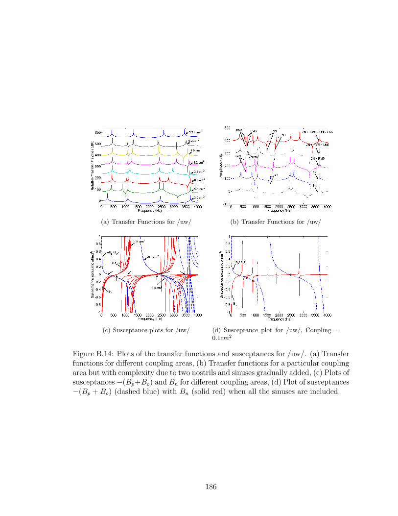
(a) Transfer Functions for /uw/ (b) Transfer Functions for /uw/

(c) Susceptance plots for /uw/ (d) Susceptance plot for /uw/, Coupling =0.1cm2

Figure B.14: Plots of the transfer functions and susceptances for /uw/. (a) Transferfunctions for different coupling areas, (b) Transfer functions for a particular couplingarea but with complexity due to two nostrils and sinuses gradually added, (c) Plots ofsusceptances −(Bp+Bo) and Bn for different coupling areas, (d) Plot of susceptances−(Bp + Bo) (dashed blue) with Bn (solid red) when all the sinuses are included.

186

(a) Spectrogram of boo (b) Spectrogram of boon

(c) Non-nasalized /uw/ (d) Nasalized /uw/

Figure B.15: Comparison of oral and nasalized vowels and their real and simulatedacoustic spectra. (a) Spectrogram of the word boo. (b) Spectrogram of the wordboon. (c) A frame of spectrum taken at 0.2s (in solid blue), F1 = 285 Hz, F2 =877 Hz, F3 = 2469 Hz, F4 = 3449 Hz, F5 = 4040 Hz; Simulated spectrum fornon-nasalized /uw/ with losses (in dashed black). (d) A frame of spectrum takenat 0.30s (in solid blue), F1 = 225 Hz, F2 = 1040 Hz, F3 = 2612 Hz, F4 = 3632 Hz,Frequencies of extra peaks = 775 Hz and 2204 Hz; Simulated spectrum for nasalized/uw/ with losses (in dashed black). Simulated spectra generated at a coupling of0.1 cm2.

187

(a) Spectrogram of woo (b) Spectrogram of womb

(c) Non-nasalized /uw/ (d) Nasalized /uw/

Figure B.16: Comparison of oral and nasalized vowels and their real and simulatedacoustic spectra. (a) Spectrogram of the word woo. (b) Spectrogram of the wordwomb. (c) A frame of spectrum taken at 0.16 s (in solid blue), F1 = 265 Hz, F2= 898 Hz, F3 = 2449 Hz, F4 = 3387 Hz, F5 = 3836 Hz; Simulated spectrum fornon-nasalized /uw/ with losses (in dashed black). (d) A frame of spectrum taken at0.23s (in solid blue), F1 = 245 Hz, F2 = 1000 Hz, F3 = 2530 Hz, F4 = 3408 Hz, F5= 3857 Hz, Frequencies of extra peaks = 734 Hz and 2245 Hz; Simulated spectrumfor nasalized /uw/ with losses (in dashed black). Simulated spectra generated at acoupling of 0.1 cm2.

188

Appendix C

Algorithm to calculate A1− P0, A1− P1, F1− Fp0, and F1− Fp1

function [p0p1APs] = getP0P1(so, F1, F2, islog)

% so = input frame spectrum

% F1 = first formant frequency

% F2 = second formant frequency

% islog = flag indicating whether the spectrum is log spectrum or not

% Note that, poles are seen in the spectrum as peaks. Therefore, all

% poles are referred to as peaks in this algorithm.

set p0Lim = 800

set p1Lim = 1500

set p0 = p1 = p0default = p1default = min(so(F1:F2))

set fp0 = fp1 = fp0default = fp1default = freq(min(so(F1:F2)))

set isP0default = 1

set isP1default = 2

set F1 = freq(peak closest to F1)

set F2 = freq(peak closest to F2)

if (F1 is not the first peak)

set (p0, fp0) = (amp, freq)(peak just below F1)

set isP0default = 0

endif

if ((F1 = F2) or there is no peak between F1 and F2)

if (there are more peaks in the spectral frame)

if (freq(peak just after F2) < p1Lim)

set (p1, fp1) = (amp, freq)(peak just after F2)

set isP1default = 0

endif

endif

elseif (there is only one peak between F1 and F2)

if ((isP0default = 1) and (freq of peak just after F1 < p0Lim))

set (p0, fp0) = (amp, freq)(peak just after F1)

set isP0default = 0

if (there are peaks after F2) and

(freq(peak just after F2) < p1Lim)

set (p1, fp1) = (amp, freq)(peak just after F2)

set isP1default = 0

189

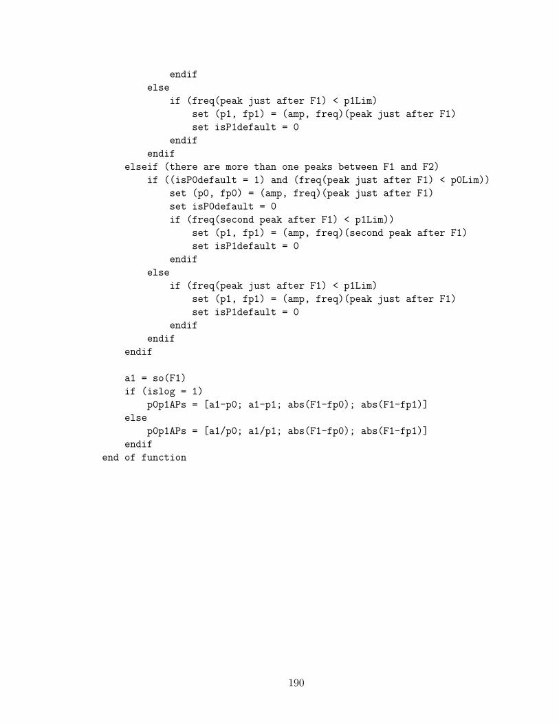
endif

else

if (freq(peak just after F1) < p1Lim)

set (p1, fp1) = (amp, freq)(peak just after F1)

set isP1default = 0

endif

endif

elseif (there are more than one peaks between F1 and F2)

if ((isP0default = 1) and (freq(peak just after F1) < p0Lim))

set (p0, fp0) = (amp, freq)(peak just after F1)

set isP0default = 0

if (freq(second peak after F1) < p1Lim))

set (p1, fp1) = (amp, freq)(second peak after F1)

set isP1default = 0

endif

else

if (freq(peak just after F1) < p1Lim)

set (p1, fp1) = (amp, freq)(peak just after F1)

set isP1default = 0

endif

endif

endif

a1 = so(F1)

if (islog = 1)

p0p1APs = [a1-p0; a1-p1; abs(F1-fp0); abs(F1-fp1)]

else

p0p1APs = [a1/p0; a1/p1; abs(F1-fp0); abs(F1-fp1)]

endif

end of function

190

BIBLIOGRAPHY

Abramson, A. S., Nye, P. W., Henderson, J., Marshall, C. W., 1981. Vowel heightand the perception of consonantal nasality. J. Acoust. Soc. Am. 70 (2), 329–339.

Ali, A. M. A., 1999. Auditory-based acoustic-phonetic signal processing for robustcontinuous speaker independent speech recognition. Ph.D. thesis, University ofPennsylvania, Philadelphia, PA, USA.

Ali, L., Gallagher, T., Goldstein, J., Daniloff, R., 1971. Perception of coarticulatednasality. J. Acoust. Soc. Am. 49 (2), 538–540.

Allen, J. B., 1994. How do humans process and recognize speech? IEEE Transactionson Speech and Audio Processing 2 (4), 567–577.

Alwan, A., Narayanan, S., Haker, K., 1997. Toward articulatory-acoustic modelsfor liquid approximants based on MRI and EPG data. Part II. The Rhotics. J.Acoust. Soc. Am. 101 (2), 1078–1089.

Arai, T., 2004. Formant shifts in nasalization of vowels. J. Acoust. Soc. Am. 115 (5),2541.

Arai, T., 2005. Comparing tongue positions of vowels in oral and nasal contexts. In:Proceedings of Interspeech. Lisbon, Portugal, pp. 1033–1036.

Baer, T., Gore, J. C., Gracco, L. C., Nye, P. W., 1991. Analysis of vocal tract shapeand dimensions using magnetic resonance imaging: Vowels. J. Acoust. Soc. Am.90 (2), 799–828.

Beddor, P. S., 1993. Phonetics and Phonology: Nasals, Nasalization and the Velum.Academic Press, Ch. The perception of nasal vowels, pp. 171–196.

Beddor, P. S., Hawkins, S., 1990. The influence of spectral prominence on perceivedvowel quality. J. Acoust. Soc. Am. 87 (6), 2684–2704.

Beddor, P. S., Strange, W., 1982. Cross language study of perception of the oral-nasal distinction. J. Acoust. Soc. Am. 71 (6), 1551–1561.

Bitar, N. N., 1997a. Acoustic analysis and modeling of speech based on phoneticfeatures. Ph.D. thesis, Boston University, Boston, MA, USA.

Bognar, E., Fujisaki, H., 1986. Analysis, synthesis and perception of French nasalvowels. In: Proceedings of ICASSP. pp. 1601–1604.

Bond, Z. S., 1975. Identification of vowels excerpted from neutral and nasal contexts.J. Acoust. Soc. Am. 59 (5), 1229–1232.

Brehm, F. E., 1922. Speech correction. Am. Ann. Deaf 67, 361–370.

191

Burges, C. J. C., 1998. A tutorial on support vector machines for pattern recognition.Data Mining and Knowledge Discovery 2 (2), 121–167.

Cairns, D. A., Hansen, J. H. L., Kaiser, J. F., 1996a. Recent advances in hypernasalspeech detection using the nonlinear teager energy operator. In: Proceedings ofICSLP. pp. 780–783.

Cairns, D. A., Hansen, J. H. L., Riski, J. E., 1994. Detection of hypernasal speechusing a nonlinear operator. In: Proceedings of IEEE Conference on Engineeringin Medicine and Biology Society. pp. 253–254.

Cairns, D. A., Hansen, J. H. L., Riski, J. E., 1996b. A noninvasive technique fordetecting hypernasal speech using a nonlinear operator. IEEE Transactions onBiomedical Engineering 43 (1), 35–45.

Chen, M. Y., 1995. Acoustic parameters of nasalized vowels in hearing-impaired andnormal-hearing speakers. J. Acoust. Soc. Am. 98 (5), 2443–2453.

Chen, M. Y., February 1996. Acoustic correlates of nasality in speech. Ph.D. thesis,MIT, Cambridge, MA, USA.

Chen, M. Y., 1997. Acoustic correlates of English and French nasalized vowels. J.Acoust. Soc. Am. 102 (4), 2360–2370.

Chen, M. Y., 2000a. Acoustic analysis of simple vowels preceding a nasal in StandardChinese. Journal of Phonetics 28 (1), 43–67.

Chen, M. Y., 2000b. Nasal detection module for a knowledge-based speech recogni-tion system. In: Proceedings of ICSLP. Vol. IV. Beijing, China, pp. 636–639.

Chomsky, N., Halle, N., 1968. The sound pattern of English. Harper and Row.

Dang, J., Honda, K., 1995. An investigation of the acoustic characteristics of theparanasal cavities. In: Proceedings of the XIIIth International Congress of Pho-netic Sciences. pp. 342–345.

Dang, J., Honda, K., 1996. Acoustic characteristics of the human paranasal sinusesderived from transmission characteristic measurement and morphological obser-vation. J. Acoust. Soc. Am. 100 (5), 3374–3383.

Dang, J., Honda, K., 1997. Acoustic characteristics of the piriform fossa in modelsand humans. J. Acoust. Soc. Am. 101 (1), 456–465.

Dang, J., Honda, K., Suzuki, H., 1994. Morphological and acoustical analysis of thenasal and the paranasal cavities. J. Acoust. Soc. Am. 96 (4), 2088–2100.

Delattre, P., Monnot, M., 1968. The role of duration in the identification of Frenchnasal vowels. International Review of Applied Linguistics 6, 267–288.

192

Deng, L., Cui, X., Pruvenok, R., Huang, J., Momen, S., Chen, Y., Alwan, A., 2006.A database of vocal tract resonance trajectories for research in speech processing.In: Proceedings of ICASSP. pp. 369–372.

Deshmukh, O., August 2006. Synergy of acoustic-phonetics and auditory modelingtowards robust speech recognition. Ph.D. thesis, University of Maryland, CollegePark, MD, USA.

Dickson, D. R., 1962. Acoustic study of nasality. J. of Speech and Hearing Research5 (2), 103–111.

Fant, G., 1960. Acoustic Theory of Speech Production. Mouton, The Hague, Nether-lands.

Fant, G., 1979b. Vocal source analysis - a progress report. STL-QPSR 20 (3-4),31–53.

Feng, G., Castelli, E., 1996. Some acoustic features of nasal and nasalized vowels:A target for vowel nasalization. J. Acoust. Soc. Am. 99 (6), 3694–3706.

Fujimura, O., Lindqvist, J., 1971. Sweep tone measurements of vocal-tract charac-teristics. J. Acoust. Soc. Am. 49, 541–558.

Glass, J., Chang, J., McCandless, M., 1996. A probabilistic framework for feature-based speech recognition. In: Proceedings of ICSLP. pp. 2277–2280.

Glass, J. R., 1984. Nasal consonants and nasalised vowels: An acoustical study andrecognition experiment. Master’s thesis, MIT, Cambridge, MA, USA.

Glass, J. R., Zue, V. W., 1985. Detection of nasalized vowels in American English.In: Proceedings of ICASSP. pp. 1569–1572.

Glenn, J. W., Kleiner, N., 1968. Speaker identification based on nasal phonation. J.Acoust. Soc. Am. 43 (2), 368–372.

Godfrey, J. J., Holliman, E. C., McDaniel, J., 1992. SWITCHBOARD: telephonespeech corpus for research and development. In: Proceedings of ICASSP. pp.517–520.

Greenberg, S., 1999. Speaking in shorthand: A syllable-centric perspective for un-derstanding pronunciation variation. Speech Communication 29 (2), 159–176.

Greenberg, S., 2005. Listening to Speech: An auditory perspective. Lawrence Earl-baum Associates, Ch. A Multi-Tier framework for understanding spoken language.

Hajro, N., April 2004. Automated nasal feature detection for the lexical access fromfeatures project. Master’s thesis, MIT, Cambridge, MA, USA.

193

Hasegawa-Johnson, M., Baker, J., Borys, S., Chen, K., Coogan, E., Greenberg, S.,Juneja, A., Kirchoff, K., Livescu, K., Mohan, S., Muller, J., Sonmez, K., Wang,T., 2004. Landmark-based speech recognition: Report of the 2004 Johns Hopkinssummer workshop. Tech. rep.

Hasegawa-Johnson, M., Baker, J., Borys, S., Chen, K., Coogan, E., Greenberg, S.,Juneja, A., Kirchoff, K., Livescu, K., Mohan, S., Muller, J., Sonmez, K., Wang,T., 2005. Landmark-based speech recognition: Report of the 2004 Johns Hopkinssummer workshop. In: Proceedings of ICASSP. pp. 213–216.

Hattori, S., Yamamoto, K., Fujimura, O., 1958. Nasalization of vowels in relationto nasals. J. Acoust. Soc. Am. 30 (4), 267–274.

Hawkins, S., Stevens, K. N., 1985. Acoustic and perceptual correlates of the non-nasal-nasal distinction for vowels. J. Acoust. Soc. Am. 77 (4), 1560–1575.

Hegde, R. M., Murthy, H. A., Ramana Rao, G. V., 2004. Application of the modifiedgroup delay function to speaker identification and discrimination. In: Proceedingsof ICASSP. pp. 517–520.

Hegde, R. M., Murthy, H. A., Ramana Rao, G. V., 2005. Speech processing usingjoint features derived from the modified group delay function. In: Proceedings ofICASSP. pp. 541–544.

Honda, K., Takemoto, H., Kitamura, T., Fujita, S., Takano, S., 2004. Exploringhuman speech production mechanisms by MRI. IEICE Trans. Inf. and Syst. E87-D (5), 1050–1058.

House, A. S., Stevens, K. N., 1956. Analog studies of the nasalization of vowels. J.of Speech and Hearing Disorders 21 (2), 218–232.

Huffman, M. K., 1990. The role of F1 amplitude in producing nasal percepts. J.Acoust. Soc. Am. 88 (S1), S54.

Joachims, T., 1999. Advances in Kernel Methods - Support Vector Learning. MITPress, Ch. Making large-Scale SVM Learning Practical.

Juneja, A., December 2004. Speech recognition based on phonetic features andacoustic landmarks. Ph.D. thesis, University of Maryland, College Park, MD,USA.

Juneja, A., Espy-Wilson, C., 2002. Segmentation of continuous speech usingacoustic-phonetic parameters and statistical learning. In: Proceedings of 9th In-ternational Conference on Neural Information Processing. Vol. 2. Singapore, pp.726–730.

Juneja, A., Espy-Wilson, C., 2003. Speech segmentation using probabilistic phoneticfeature hierarchy and support vector machines. In: Proceedings of InternationalJoint Conference on Neural Networks. Portland, Oregon.

194

Kahn, D., 1976. Syllable-based generalizations in English phonology. Ph.D. thesis,MIT, Cambridge, MA, USA.

Kawasaki, H., 1986. Experimental Phonology. Academic Press, Ch. Phonetic expla-nation for phonological universals: The case of distinctive vowel nasalization, pp.81–103.

Klatt, D. H., 1980. Software for cascade/parallel formant synthesizer. J. Acoust.Soc. Am. 67 (3), 971–995.

Klatt, D. H., Klatt, L. C., 1990. Analysis, synthesis, and perception of voice qualityvariations among female and male talkers. J. Acoust. Soc. Am. 87 (2), 820–857.

Krakow, R. A., 1993. Phonetics and Phonology: Nasals, Nasalization and the Velum.Academic Press, Ch. Nonsegmental influences on velum movement patterns: Syl-lables, Sentences, Stress and Speaking Rate, pp. 87–116.

Krakow, R. A., Beddor, P. S., 1991. Coarticulation and the perception of nasality. In:Proceedings of the 12th International Congress of Phonetic Sciences. pp. 38–41.

Krakow, R. A., Beddor, P. S., Goldstein, L. M., Fowler, C., 1988. Coarticulatoryinfluences on the perceived height of nasal vowels. J. Acoust. Soc. Am. 83 (3),1146–1158.

Ladefoged, P., 1982. A course in phonetics. Harcourt Brace Jovanovich.

Lahiri, A., Marslen-Wilson, W., 1991. The mental representation of lexical form: Aphonological approach to the recognition lexicon. Cognition 38 (3), 245–294.

Lindqvist-Gauffin, J., Sundberg, J., 1976. Acoustic properties of the nasal tract.Phonetica 33 (3), 161–168.

Lintz, L. B., Sherman, D., 1961. Phonetic elements and perception of nasality. Jour-nal of Speech and Hearing Research 4, 381–396.

Lippman, R. P., 1997. Speech recognition by machines and humans. Speech Com-munication 22, 1–15.

Liu, S. A., 1996. Landmark detection for distinctive feature-based speech recogni-tion. J. Acoust. Soc. Am. 100 (5), 3417–3430.

Maddieson, I., 1984. Patterns of Sounds. Cambridge University Press, Cambridge.

Maeda, S., 1982a. A digital simulation method of the vocal-tract system. SpeechCommunication 1, 199–229.

Maeda, S., 1982b. The role of the sinus cavities in the production of nasal vowels.In: Proceedings of ICASSP. Vol. 2. pp. 911–914.

195

Maeda, S., 1982c. Acoustic cues for vowel nasalization: A simulation study. J.Acoust. Soc. Am. 72 (S1), S102.

Maeda, S., 1993. Phonetics and Phonology: Nasals, Nasalization and the Velum.Academic Press, Ch. Acoustics of vowel nasalization and articulatory shifts inFrench Nasal Vowels, pp. 147–167.

Mermelstein, P., 1975. Automatic segmentation of speech into syllabic units. J.Acoust. Soc. Am. 58 (4), 880–883.

Mesgarani, N., Slaney, M., Shamma, S., 2004. Speech discrimination based on mul-tiscale spectrotemporal features. In: Proceedings of ICASSP. pp. 601–604.

Mohr, B., Wang, W. S.-Y., 1968. Perceptual distance and the specification of phono-logical features. Phonetica 18, 31–45.

Moore, C. A., 1992. The correspondence of vocal tract resonance with volumes ob-tained from magnetic resonance imaging. Journal of Speech and Hearing Research35, 1009–1023.

Murthy, H. A., Gadde, V., 2003. The modified group delay function and its appli-cation to phoneme recognition. In: Proceedings of ICASSP. pp. 68–71.

Muthusamy, Y. K., Cole, R. A., Oshika, B. T., 1992. The OGI multi-languagetelephone speech corpus. In: Proceedings of ICSLP. Banff, Alberta, Canada.

Narayanan, S., Alwan, A., Haker, K., 1995. An articulatory study of fricative conso-nants using magnetic resonance imaging. J. Acoust. Soc. Am. 98 (3), 1325–1347.

Narayanan, S., Alwan, A., Haker, K., 1997. Toward articulatory-acoustic modelsfor liquid approximants based on MRI and EPG data. Part I. The Laterals. J.Acoust. Soc. Am. 101 (2), 1064–1077.

Niu, X., Kain, A., Van Santen, J. P. H., 2005. Estimation of the acoustic propertiesof the nasal tract during the production of nasalized vowels. In: Proceedings ofInterspeech. Lisbon, Portugal, pp. 1045–1048.

Ohala, J. J., 1971. Monitoring soft palate movements in speech. J. Acoust. Soc. Am.50 (1A), 140.

Prahler, A., 1998. Analysis and synthesis of American English lateral consonant.Master’s thesis, MIT, Cambridge, MA, USA.

Pruthi, T., Espy-Wilson, C., 2003. Automatic classification of nasals and semivowels.In: Proceedings of 15th International Congress of Phonetic Sciences (ICPhS).Barcelona, Spain, pp. 3061–3064.

Pruthi, T., Espy-Wilson, C., 2004a. Acoustic parameters for automatic detection ofnasal manner. Speech Communication 43 (3), 225–239.

196

Pruthi, T., Espy-Wilson, C., 2004b. Advances in the acoustic correlates of nasalsfrom analysis of MRI data. J. Acoust. Soc. Am. 115 (5), 2543.

Pruthi, T., Espy-Wilson, C., 2005. Simulating and understanding the effects of velarcoupling area on nasalized vowel spectra. J. Acoust. Soc. Am. 118 (3), 2024.

Pruthi, T., Espy-Wilson, C., 2006a. Acoustic parameters for nasality based on amodel of the auditory cortex. J. Acoust. Soc. Am. 119 (5), 3338.

Pruthi, T., Espy-Wilson, C., 2006b. Automatic detection of vowel nasalization usingknowledge-based acoustic parameters. J. Acoust. Soc. Am. 120 (5), 3377.

Pruthi, T., Espy-Wilson, C., 2006c. An MRI based study of the acoustic effects ofsinus cavities and its application to speaker recognition. In: Interspeech. Pitts-burgh, Pennsylvania, pp. 2110–2113.

Ruhlen, M., 1978. Universals of Human Language: Vol 2, Phonology. Stanford Uni-versity Press, Ch. Nasal Vowels, pp. 203–242.

Seaver, E. J., Dalston, R. M., Leeper, H. A., Adams, L. E., 1991. A study ofnasometric values for normal nasal resonance. Journal of Speech and HearingResearch 34 (4), 715–721.

Stevens, K. N., 1989. On the quantal nature of speech. Journal of Phonetics 17,3–45.

Stevens, K. N., 1998. Acoustic Phonetics. MIT Press, Cambridge, Massachusetts.

Stevens, K. N., Andrade, A., Viana, M. C., 1987a. Perception of vowel nasalizationin VC contexts: A cross-language study. J. Acoust. Soc. Am. 82 (S1), S119.

Stevens, K. N., Fant, G., Hawkins, S., 1987b. In Honor of Ilse Lehiste. Foris Publica-tions, Ch. Some acoustical and perceptual correlates of nasal vowels, pp. 241–254.

Story, B. H., 1995. Physiologically-based speech simulation using an enhanced wave-reflection model of the vocal tract. Ph.D. thesis, University of Iowa, Iowa city, IA,USA.

Story, B. H., Titze, I. R., Hoffman, E. A., 1996. Vocal tract area functions frommagnetic resonance imaging. J. Acoust. Soc. Am. 100 (1), 537–554.

Talkin, D., 1987. Speech formant trajectory estimation using dynamic programmingwith modulated transition costs. J. Acoust. Soc. Am. 82 (S1), S55.

TIMIT, 1990. TIMIT acoustic-phonetic continuous speech corpus, national instituteof standards and technology speech disc 1-1.1, NTIS Order No. PB91-5050651996,october 1990.

Vapnik, V. N., 1995. Nature of Statistical Learning Theory. Springer-Verlag.

197

Vijayalakshmi, P., Reddy, M. R., 2005a. Detection of hypernasality using statisticalpattern classifiers. In: Proceedings of Interspeech. Lisbon, Portugal, pp. 701–704.

Vijayalakshmi, P., Reddy, M. R., 2005b. The analysis of band-limited hypernasalspeech using group delay based formant extraction technique. In: Proceedings ofInterspeech. Lisbon, Portugal, pp. 665–668.

Whalen, D. H., Beddor, P. S., 1989. Connections between nasality and vowel dura-tion and height: Elucidation of the Eastern Algonquian intrusive nasal. Language65, 457–486.

Wright, J. T., 1986. Experimental Phonology. Academic Press, Ch. The bahavior ofnasalized vowels in the perceptual vowel space, pp. 45–67.

Yegnanarayana, B., 1978. Formant extraction from linear-prediction phase spectra.J. Acoust. Soc. Am. 63 (5), 1638–1640.

Zhang, Z., Espy-Wilson, C. Y., 2004. A vocal-tract model of American English /l/.J. Acoust. Soc. Am. 115 (3), 1274–1280.

Zheng, Y., Hasegawa-Johnson, M., 2004. Formant tracking by mixture state particlefilter. In: Proceedings of ICASSP. pp. 565–568.

Zue, V., Seneff, S., Glass, J., 1990. Speech database development at MIT: TIMITand beyond. Speech Communication 9 (4), 351–356.

198