Abrasive Blasting with Post-Process and In-Situ Characterization

Robert Jeffrey Mills

Thesis submitted to the faculty of the Virginia Polytechnic Institute and State University

in partial fulfillment of the requirements for the degree of

Master of Science

In

Materials Science and Engineering

Gary R. Pickrell, Chair

Daniel S. Homa

Alan P. Druschitz

Thomas W. Staley

May 29, 2014

Blacksburg, VA

Keywords: (abrasive blasting, media, substrate, roughness, profilometry, temperature,

optical fibers,)

Copyright 2014, Robert J. Mills

Abrasive Blasting with Post-Process and In-Situ Characterization

Robert Jeffrey Mills

ABSTRACT

Abrasive blasting is a common process for cleaning or roughening the surface of a

material prior to the application of a coating. Although the process has been in practice for

over 100 years, the lack of a comprehensive understanding of the complex interactions that

exist with the process can still yield an inferior surface quality. Subsequently, parts can be

rejected at one of many stages of the manufacturing process and/or fail unexpectedly upon

deployment. The objective of this work is to evaluate the effect of selected input

parameters on the characteristics of the blasted surface characteristics so that a more useful

control strategy can be implemented. To characterize surface roughness, mechanical

profilometry was used to collect average roughness parameter, Ra. Decreasing blast

distance from 6” to 4” gave ΔRa = +0.22 µm and from 8” to 6” gave ΔRa = +0.22 µm.

Increasing blast pressure from 42 psi to 60 psi decreased the Ra by 0.33 µm. Media

pulsation reduced Ra by 0.56 µm and the use of new media reduced Ra by 0.47 µm.

Although blasting under the same conditions and operator on different days led to ΔRa due

to shorter blast times, there was no statistically significant variance in Ra attributed to

blasting on different days. Conversely, a ΔRa = +0.46 µm was observed upon blasting

samples with different cabinets. No significant ΔRa was found when switching between

straight and Venturi nozzles or when using different operators.

Furthermore, the feasibility of fiber optic sensing technologies was investigated as

potential tools to provide real time feedback to the blast machine operator in terms of

substrate temperature. Decreasing the blast distance from 6” to 4” led to ΔT = +9.2 °C,

while decreasing the blast angle to 45° gave ΔT= -11.6 °C for 304 stainless steel substrates.

Furthermore, increasing the blast pressure from 40 psi to 50 psi gave ΔT= +15.3 °C and

changing from 50 psi to 60 psi gave ΔT= +9.9 °C. The blast distance change from 8” to 6”

resulted in ΔT = +9.8 °C in thin stainless steel substrate temperature. The effects of

substrate thickness or shape were evaluated, giving ΔT= +7.4 °C at 8” distance, ΔT= +20.2

°C at 60 psi pressure, and ΔT= -15.2 °C at 45° blasting when comparing thin stainless steel

against 304 stainless steel (thick) temperatures. No significant ΔT in means was found

when going from 6” to 8” distance on 304 stainless steel, 40 psi and 60 psi blasting of thin

iii

SS, as well as angled and perpendicular blasting of thin SS. Comparing thick 304 and thin

stainless steel substrates at a 6” blast distance gave no significant ΔT.

iv

Acknowledgements I would like to sincerely thank Dr. Gary Pickrell for his support, feedback, and allowing

me to work in his research group these past four semesters. I have learned many things from

working in his lab and with his research team. I’m appreciative of the support of Dr. Daniel Homa

for his patience, encouragement, and inspiring work ethic on various research projects. I have

increased my knowledge of abrasive blasting and optical fiber technologies through experiments

in this research group also.

I would like to thank specific members of the research team. I want to thank Edward, Cary,

and Taylor for helping me carry out experiments in the blast cabinet in the Hancock Lab. Their

time and patience were invaluable and helped me obtain some of experimental results shown in

this report. I appreciate the rest of the research team being cooperative and helpful when I used the

blast cabinet, as it was loud and annoying at times.

Lastly, I want to thank everyone who helped me make it this far in my academic career.

Without the support, encouragement, and love from my parents schoolwork, research, and thesis

writing would not have been possible. My friends and other family helped encourage me along the

way and I’m grateful for that as well.

I would also like to acknowledge and thank CCAM for their funding of the equipment and

materials for the roughness testing portion of this work. I want to thank Norton Sandblasting as

well for answering many questions related to maintaining the blasting equipment. LISA helped

greatly with the statistical analysis of the results as well.

All photographs by author (Robert J. Mills), 2014.

v

Table of Contents

1 Introduction ............................................................................................................................1 1.1 Motivation ........................................................................................................................... 1

1.2 Research Approach ............................................................................................................. 2

1.3 Thesis Scope and Organization ........................................................................................... 2

2 Background ............................................................................................................................4 2.1 Abrasive Blasting History and Advances ........................................................................... 4

2.1.1 Various Blasting Methods............................................................................................ 5

2.1.2 Control Systems ........................................................................................................... 6

2.2 Abrasive Media ................................................................................................................... 7

2.2.1 Abrasive Shape ............................................................................................................ 7

2.2.2 Grit, Shot and Cylindrical .......................................................................................... 10

2.2.3 Abrasive Size & Size Distribution ............................................................................. 11

2.2.4 Abrasive Hardness ..................................................................................................... 14

2.2.5 Abrasive Density ........................................................................................................ 16

2.2.6 Type (Metallic vs. Non-Metallic) .............................................................................. 17

2.2.7 Fracture Strength ........................................................................................................ 18

2.2.8 Impurities ................................................................................................................... 19

2.3 Substrates .......................................................................................................................... 19

2.3.1 Substrate Material ...................................................................................................... 20

2.3.2 Substrate Hardness ..................................................................................................... 21

2.3.3 Substrate Thickness ................................................................................................... 21

2.3.4 Substrate Shape .......................................................................................................... 21

2.3.5 Initial Surface Roughness .......................................................................................... 22

2.3.6 Pre-Blasting Strains and Stresses ............................................................................... 23

2.3.7 Cleanliness ................................................................................................................. 23

2.4 Blasting Environment ....................................................................................................... 24

2.4.1 Temperature ............................................................................................................... 24

2.4.2 Humidity .................................................................................................................... 25

2.5 Blasting Process Parameters ............................................................................................. 26

2.5.1 Blasting Pressure and Media Flow Rate .................................................................... 26

2.5.2 Stand-off Distance ..................................................................................................... 27

2.5.3 Blast Angle................................................................................................................. 29

2.5.4 Blast Time .................................................................................................................. 30

2.5.5 Media Degradation/Fragmentation ............................................................................ 32

vi

2.5.6 Nozzle Type ............................................................................................................... 33

2.6 Characterization Techniques ............................................................................................. 34

2.6.1 Mechanical Profilometry ........................................................................................... 34

2.6.2 Optical Profilometry/Microscopy .............................................................................. 36

3 Experimental Methods ........................................................................................................37 3.1 Roughness Experimental Procedure ................................................................................. 37

3.1.1 Media, Substrate, and Parameter Selections .............................................................. 37

3.1.2 Cabinet Information ................................................................................................... 38

3.1.3 Substrate Preparation ................................................................................................. 39

3.1.4 Cabinet Preparation and Substrate Blasting ............................................................... 40

3.2 Post-Process Characterization ........................................................................................... 43

3.2.1 Mitutoyo Surftest SJ-210 Mechanical Profilometer .................................................. 43

3.2.2 HIROX Optical Microscopy ...................................................................................... 44

3.2.3 UVA ROST Optical Profilometry ............................................................................. 44

3.3 Substrate Temperature Experimental Procedure .............................................................. 45

3.3.1 Optical Fiber Splicing, Adaptors, and Connectors .................................................... 45

3.3.2 Optical Fiber Connection Cleanliness ....................................................................... 46

3.3.3 Micron Optics SM125 Optical Sensing Interrogator ................................................. 47

3.3.4 Temperature Sensor and Probe .................................................................................. 47

3.3.5 Micron Optics Enlight Software ................................................................................ 48

3.3.6 Sensor Attachment to Substrates ............................................................................... 50

3.3.7 Temperature Blast Conditions ................................................................................... 52

3.4 Statistical Analysis of Roughness and Temperature Data ................................................ 52

4 Results and Discussion .........................................................................................................54 4.1 Roughness Characterization Results ................................................................................... 54

4.2 Effect of Process Parameters on Surface Roughness ........................................................ 56

4.3 Repeatability and Reproducibility .................................................................................... 60

4.4 Temperature Sensor Measurements .................................................................................. 62

4.5 Temperature Probe Measurements ................................................................................... 64

5 Conclusions ...........................................................................................................................71

6 Future Work .........................................................................................................................73 References .....................................................................................................................................74

Appendices ....................................................................................................................................78 Appendix A Blast Media Chart................................................................................................. 78

Appendix B Nozzle Design ...................................................................................................... 79

Appendix C Roughness Testing Information ........................................................................... 80

vii

Appendix D Temperature Testing Information ........................................................................ 83

Appendix E Sample F-test and t-test calculations .................................................................... 87

Appendix F Roughness F-tests and t-tests Data ....................................................................... 89

Appendix G Temperature F-tests and t-tests data ..................................................................... 92

Appendix H Figures and Tables Permissions ........................................................................... 96

viii

List of Tables Table 2-1 ISO 12944-4 Blast cleaning methods. Momber A. Blast Cleaning Technology:

Chapter 1: Introduction, 2008. p. 3. http://link.springer.com/chapter/10.1007%2F978-3-540-

73645-5_2 (accessed March 31, 2013) Used with permission from Copyright Clearance Center,

2014................................................................................................................................................. 5 Table 2-2 Mohs hardness scale. Momber A. Blast Cleaning Technology: Chapter 2: Abrasive

Materials, 2008. p. 14. http://link.springer.com/chapter/10.1007%2F978-3-540-73645-5_2

(accessed April 1, 2013) Used with permission from Copyright Clearance Center, 2014. .......... 14

Table 3-1 Media and substrate properties. .................................................................................... 38 Table 3-2 Cabinet specifications for roughness testing. ............................................................... 38

Table 3-3 Blasting information during one experiment. ............................................................... 40

Table 3-4 Experimental design sets for roughness testing............................................................ 40 Table 3-5 Measurement information for roughness testing. ......................................................... 43 Table 3-6 SJ-210 measurement settings. ...................................................................................... 43 Table 3-7 Experimental design sets for temperature testing. ........................................................ 52

Table 4-1 SJ-210 Ra results with three types of standard deviation. ............................................ 54 Table 4-2 Hirox measurements for Sa & σ calculations of samples 2.10 and 3.10. ..................... 55

Table 4-3 ROST Avg. Sa and measurement σ values. ................................................................. 55 Table 4-4 Comparison of Ra and σM for characterization techniques. .......................................... 56 Table 4-5 304 Stainless steel substrate temperature results. ......................................................... 66

Table 4-6 Thin stainless steel substrate temperature results. ........................................................ 68

Table A-1 Blast media chart. No Author. “Blast Media Chart.” Norton Sandblasting Equipment.

2014. http://www.nortonsandblasting.com/nsbabrasives.html (accessed June 9, 2014) Used with

permission from Norton Sandblasting Equipment, 2014. ............................................................. 78

ix

List of Figures Figure 2.1 a. pre-blasting, b. blasting, and c. post-blasting surfaces. No Author. “Technical

Reference: Surface Preparation.” Blast One. 2014. http://www.blast-one.com/weekly-tips/the-

difference-between-surface-profile-and-class-of-blast (accessed May 14, 2014) Used with

permission from Blast One, 2014. .................................................................................................. 4 Figure 2.2 Suction and pressure blasting systems. No Author. “Blast Cabinets.” Norton

Sandblasting Equipment, 2014. http://www.nortonsandblasting.com/nsbcontact.html (accessed

May 14, 2014) Used with permission from Norton Sandblasting Equipment, 2014. ..................... 6

Figure 2.3 Media shape definitions; a. shape factor & circulatory factor, b. roundness, &

sphericity, & c. elongation ratio & flatness ratio. Momber A. Blast Cleaning Technology:

Chapter 2: Abrasive Materials, 2008. p. 19. http://link.springer.com/chapter/10.1007%2F978-3-

540-73645-5_2 (accessed March 31, 2013) Used with permission from Copyright Clearance

Center, 2014. ................................................................................................................................... 8 Figure 2.4 a. Hansink’s shape designations & b. garnet roundness-sphericity chart. Momber A.

Blast Cleaning Technology: Chapter 2: Abrasive Materials, 2008. p. 21. http://link.springer.com/

chapter/10.1007%2F978-3-540-73645-5_2 (accessed March 31, 2013) Used with permission

from Copyright Clearance Center, 2014. ........................................................................................ 9

Figure 2.5 Shape, size, and type relationships. Momber A. Blast Cleaning Technology: Chapter

2: Abrasive Materials, 2008. p. 20. http://link.springer.com/chapter/10.1007%2F978-3-540-

73645-5_2 (accessed March 31, 2013) Used with permission from Copyright Clearance Center,

2014............................................................................................................................................... 10

Figure 2.6 a. Grit image and b. shot image. Momber A. Blast Cleaning Technology: Chapter 2:

Abrasive Materials, 2008. p. 18. http://link.springer.com/chapter/10.1007%2F978-3-540-73645-

5_2 (accessed March 31, 2013) Used with permission from Copyright Clearance Center, 2014. 10

Figure 2.7 Distribution of sieve analysis. Momber A. Blast Cleaning Technology: Chapter 2:

Abrasive Materials, 2008. p. 26. http://link.springer.com/chapter/10.1007%2F978-3-540-73645-

5_2 (accessed March 31, 2013) Used with permission from Copyright Clearance Center, 2014. 12 Figure 2.8 Grit contamination vs. roughness. Day, James; Huang, Xiao; and Richards, N.L.

“Examination of a Grit-Blasting Process for Thermal Spraying Using Statistical Methods.”

Journal of Thermal Spray Technology, 2005/Vol. 14, p. 477.

http://link.springer.com/article/10.1361%2F105996305X76469 (accessed November 2012)

Used with permission from Copyright Clearance Center, 2014. .................................................. 13 Figure 2.9 Grit diameter vs. a. residual grit and b. penetration depth. Maruyama T, Akagi K,

Kobayashi T. "Effects of Blasting Parameters on Removability of Residual Grit." Journal of

Thermal Spray Technology. 2006/Vol. 15, no. 4. p. 820.

http://link.springer.com/article/10.1361%2F105996306X147018 (accessed November 2, 2012)

Used with permission from Copyright Clearance Center; letter attached. ................................... 14 Figure 2.10 Abrasive hardness effect on specific mass loss. Momber A. Blast Cleaning

Technology: Chapter 2: Abrasive Materials, 2008. p. 11, 12.

http://link.springer.com/chapter/10.1007%2F978-3-540-73645-5_2 (accessed March 31, 2013)

Used with permission from Copyright Clearance Center, 2014. .................................................. 16

Figure 2.11 a. Steel shot, b. steel grit, c. brown corundum, & d. demetalized steel slag. Makova,

I., Sopko, M. "Effect of Blasting Material on Surface Morphology of Steel Sheets." Acta

Metallurgica Slovaca. 2010/ Vol. 16, no. 2, p. 111. (accessed March 07, 2013) Used with

permission from Acta Metallurgica Slovaca, 2014....................................................................... 17

x

Figure 2.12 Particle strength vs. a. Weibull function & b. vs. fracture strength. Momber A. Blast

Cleaning Technology: Chapter 2: Abrasive Materials, 2008. p. 11, 12. http://link.springer

.com/chapter/10.1007%2F978-3-540-73645-5_2 (accessed March 31, 2013) Used with

permission from Copyright Clearance Center, 2014]. .................................................................. 19

Figure 2.13 Temperature effects from blasting. Fang, C.K., Chuang, T.H. "Erosion of SS41

Steel by Sand Blasting." Metallurgical and Materials Transactions A. 1999/Vol. 30A, p. 944.

(accessed January 11, 2013) Used with permission from Copyright Clearance Center, 2014. .... 25 Figure 2.14 Effect of humidity during blasting. Fang, C.K., Chuang, T.H. "Erosion of SS41 Steel

by Sand Blasting." Metallurgical and Materials Transactions A. 1999/Vol. 30A, p. 944.

(accessed January 11, 2013) Used with permission from Copyright Clearance Center, 2014. .... 25

Figure 2.15 Blasting pressure vs. grit flow rate. Mellalia, M., Grimaud, A., Leger, A.C.,

Fauchais, P., and Lu, J. “Alumina Grit Blasting Parameters for Surface Preparation in the Plasma

Spraying Operation.” Journal of Thermal Spray Technology. 1997/Vol. 6. No. 2. p 219.

(accessed October 22, 2012) Used with permission from Copyright Clearance Center, 2014. .. 27 Figure 2.16 Blast pressure vs. compressive residual stress. Chander, K. Poorna, Vashita, M.,

Sabiruddin, Kazi, Paul, S., Bandyopadhyay, P.P. “Effects of Grit Blasting on Surface Properties

of Steel Substrates.” Materials and Design. 2009. p. 2901. (accessed November 2012) Used with

permission from Copyright Clearance Center, 2014. ................................................................... 27 Figure 2.17 Surface roughness distance. Chander, K. Poorna, Vashita, M., Sabiruddin, Kazi,

Paul, S., Bandyopadhyay, P.P. “Effects of Grit Blasting on Surface Properties of Steel

Substrates.” Materials and Design. 2009. p. 2899. (accessed November 2012) Used with

permission from Copyright Clearance Center, 2014. ................................................................... 28 Figure 2.18 Surface roughness vs. blasting distance/substrate type. Mellalia, M., Grimaud, A.,

Leger, A.C., Fauchais, P., and Lu, J. “Alumina Grit Blasting Parameters for Surface Preparation

in the Plasma Spraying Operation.” Journal of Thermal Spray Technology. 1997/Vol 6. No. 2. p

221. (accessed October 22, 2012) Used with permission from Copyright Clearance Center,

2014............................................................................................................................................... 29 Figure 2.19 a. Cross-sectional photographs & b. Angle vs. Ra. Amada, Shigeyasu, Hirose, Tohru.

"Influence of grit blasting pre-treatment on the adhesion strength of plasma sprayed coatings:

fractal analysis of roughness." Surface and Coatings Technology. 1998/Vol. 102. p. 134.

http://dx.doi.org/10.1016/S0257-8972(97)00628-2 (accessed October 29, 2012) Used with

permission from Copyright Clearance Center, 2014. ................................................................... 29 Figure 2.20 Erosion rate vs. incident angle. Carter, G., Bevan I.J., Katardjiev I.V., Nobes, M.J.

"The Erosion of Copper by Reflected Sandblasting Grains." Materials Science Engineering.

1991/Vol. A. no. 132. P. 232. (accessed October 22, 2012) Used with permission from Copyright

Clearance Center, 2014. ................................................................................................................ 30 Figure 2.21 Time vs. roughness for Al2O3 against stainless steel. Celik, E., Demirkiran, A.S.,

Avci, E. "Effect of Grit Blasting of Substrate on the Corrosion Behaviour of Plasma-Sprayed

Al2O3 Coatings." Surface and Coatings Technology. 1999/Vol 116-119. p. 1062. (accessed

October 29, 2012) Used with permission from Copyright Clearance Center, 2014. .................... 31

Figure 2.22 Blast time vs. grit residue. Wigren, Jan. "Technical Note: Grit Blasting as Surface

Preparation Before Plasma Spraying." Surface and Coatings Technology. 1988/Vol 34. p. 107.

(accessed January 15, 2013) Used with permission from Copyright Clearance Center, 2014. .... 32 Figure 2.23 Fracture mechanisms. Momber A. Blast Cleaning Technology: Chapter 2: Abrasive

Materials, 2008. p. 38. http://link.springer.com/chapter/10.1007%2F978-3-540-73645-5_2

(accessed March 31, 2013) Used with permission from Copyright Clearance Center, 2014. ...... 32

xi

Figure 2.24 Number of cycles vs. disintegration #, a. substrate hardness & b. slag size. Momber

A. Blast Cleaning Technology: Chapter 2: Abrasive Materials, 2008. p. 47, 48.

http://link.springer.com /chapter/10.1007%2F978-3-540-73645-5_2 (accessed March 31, 2013)

Used with permission from Copyright Clearance Center, 2014. .................................................. 33

Figure 2.25 Mechanical profilometry. Tabenkin, Alex. “The Basics of Surface Finish

Measurement.” Quality Magazine. 2014.

http://www.deterco.com/products/Mahr%20Federal/newsletter/finish_ measure_10_19_04.htm

(accessed May 14, 2014) Used with permission from Mahr Federal Inc., 2014. ......................... 35 Figure 2.26 Average roughness, Ra image. Pickrell, G., Homa, D, Mills, R. “Abrasive Blasting

Deliverable No.3.” CCAM. 2014. (accessed April 2, 2014) Used with permission from Robert

Mills, 2014. ................................................................................................................................... 35

Figure 2.27 Surface roughness for Sa. Sosale, G., Hackling S.A., and Vengallatore, S.

"Topography Analysis of Grit-Blasted and Grit-Blasted-Acid Etched Titanium Implant Surfaces

Using Multi-scale Measurements and Multi-Parameter Statistics." Journal of Materials

Research. 2011/Vol 23, Issue 10. p. 2709. (accessed June 6, 2014) Used with permission from

Copyright Clearance Center; letter attached. ................................................................................ 36 Figure 3.1 a. unclean substrate & b. clean substrate. .................................................................... 39

Figure 3.2 Example of sample labeling (experiment # followed by sample #). ........................... 39 Figure 3.3 a. Compressed air valve open & b. ball choke valve open. ......................................... 41 Figure 3.4 a. Blast pressure regulator knob/gage & b. media flow regulator/handle. .................. 42

Figure 3.5 SJ-210 surface measurement technique. ...................................................................... 44

Figure 3.6 a. Fibers before & b. after fusion splicing. .................................................................. 46 Figure 3.7 a. Fiber connectors, b. connector for blue-yellow adaptors, & c. blue-blue connection.

....................................................................................................................................................... 46

Figure 3.8 F1-7020C connector end face cleaner. ........................................................................ 47 Figure 3.9 Optical fibers connected to the SM125 Interrogator. .................................................. 47

Figure 3.10 Epoxied temperature sensor and strain gage on Al 3003 substrate. .......................... 50 Figure 3.11 a. “TempProb2” attached to 304 SS substrate & b. blast platform pre-blasting. ...... 51 Figure 3.12 a. 304 SS & b. Thin SS substrates during experiments. ............................................ 51

Figure 4.1 Blast distances effects on Ra for 4” and 6” blasting. ................................................... 57 Figure 4.2 Blast distance effects on Ra for 6” and 8” blasting. .................................................... 57

Figure 4.3 Blast pressure effect on Ra for 42 psi and 60 psi blasting.......................................... 58 Figure 4.4 Nozzle type effect on Ra. ............................................................................................ 59 Figure 4.5 Media flow effect on Ra. ............................................................................................. 59 Figure 4.6 Media Recycling effect on Ra. .................................................................................... 60

Figure 4.7 Repeatability of same blast conditions. ....................................................................... 60 Figure 4.8 Cabinet type effect on Ra. ........................................................................................... 61 Figure 4.9 Operator effect on Ra. ................................................................................................. 62 Figure 4.10 a. Good coverage & b. bad coverage. ........................................................................ 62 Figure 4.11 Adaptor effect on substrate temperature.................................................................... 63

Figure 4.12 LED and halogen effect on substrate temperature. ................................................... 63 Figure 4.13 Blast height effect on substrate temperature with “TempSens2”. ............................. 64

Figure 4.14 Experiment #1 data. ................................................................................................... 65 Figure 4.15 Zeroed temperature experiment #1 data. ................................................................... 65 Figure 4.16 Blast distance effects on 304 SS temperature changes. ............................................. 66 Figure 4.17 Pressure effect on 304 SS temperature. ..................................................................... 67

xii

Figure 4.18 Angle effect on 304 SS temperature. ......................................................................... 68 Figure 4.19 Blast distance effect on thin SS temperature. ............................................................ 69 Figure 4.20 Blast pressure effect on thin SS temperature. ............................................................ 69 Figure 4.21 Blast angle effect on thin SS temperature. ................................................................ 70

Figure B.1 Nozzle descriptions. No Author. “Abrasive Blast Nozzles.” Kennametal Inc. 2012

page 9. http://www.kennametal.com/content/dam/kennametal/kennametal/common

/Resources/Catalogs-Literature/Advanced%20Materials%20and%20Wear%20Components/B-

12-02861_KMT_Blast_ Nozzles _Catalog_EN.pdf (accessed June 9, 2014) Used with

permission from Kennametal, Inc., 2014. ..................................................................................... 79

Figure C.1 Pulsation elimination methods [71]. ........................................................................... 80

Figure C.2 SJ-210 Example sample results for SS304 7-01 V3 measurement. ............................ 81

Figure C.3 Standard deviation calculations for experiment #2. .................................................... 81 Figure C.4 Hirox Sa and standard deviation measurements and calculations. .............................. 82 Figure C.5 UVA ROST Sa and standard deviation measurements and calculations. ................... 82 Figure D.1 Optical fiber ready for fusion splicing. ....................................................................... 83

Figure D.2 “Acquisition” window of Enlight software. ............................................................... 83 Figure D.3 “Sensors” window. ..................................................................................................... 84

Figure D.4 “TempSens2” information. ......................................................................................... 84 Figure D.5 “TempProbe2” information. ....................................................................................... 85 Figure D.6 Charts window with live temperature data. ................................................................ 85

Figure D.7 Edit sensors data saving option under “Save” window. ............................................. 86

Figure D.8 Thin stainless steel substrate (0.09” x 1.378” x 4.2875”) pre-blasting. ..................... 86 Figure E.1 Sample Fcalc and tcalc for F-test and t-test for 4” and 6” blasts on Ra comparison. ..... 87 Figure E.2 Sample Fcalc and tcalc for F-test and t-test for 4” and 6” blasts on 304 SS T comparison.

....................................................................................................................................................... 87 Figure F.1 F-test and t-test results for 4” and 6” blasts on Ra comparison. ................................. 89

Figure F.2 F-test and t-test results for 6” and 8” Ra comparison. ................................................ 89 Figure F.3 F-test and t-test results for 42 psi and 60 psi Ra comparison. ..................................... 89 Figure F.4 F-test and t-test results for 5/16” straight and 3/16” Venturi nozzle Ra comparison. . 90

Figure F.5 F-test and t-test results for no pulsation and pulsation Ra comparison. ...................... 90 Figure F.6 F-test and t-test results for newer media and old (recycled media) Ra comparison. .. 90

Figure F.7 F-test and t-test results for Day A and Day B Ra comparison. ................................... 91 Figure F.8 F-test and t-test results for VT and CCAM cabinet Ra comparison. .......................... 91 Figure F.9 F-test and t-test results for Operator A and Operator B Ra comparison. .................... 91 Figure G.1 F-test and t-test results for 4” and 6” blasts on 304 SS temperature comparison. ...... 92

Figure G.2 F-test and t-test results for 6” and 8” blasts on 304 SS temperature comparison. ...... 92 Figure G.3 F-test and t-test results for 40 psi and 50 psi blasts on 304 SS temperature

comparison. ................................................................................................................................... 92 Figure G.4 F-test and t-test results for 50 psi and 60psi blasts on 304 SS temperature comparison.

....................................................................................................................................................... 93

Figure G.5 F-test and t-test results for 45°and 90° blasts on 304 SS temperature comparison. ... 93 Figure G.6 F-test and t-test results for 6” and 8” blasts on thin SS temperature comparison. ..... 93

Figure G.7 F-test and t-test results for 40 psi and 60 psi blasts on thin SS temperature

comparison. ................................................................................................................................... 94 Figure G.8 F-test and t-test results for 45°and 90° blasts on thin SS temperature comparison. ... 94 Figure G.9 F-test and t-test results for 6”, 40 psi blasts of both substrates for T comparison. ..... 94

xiii

Figure G.10 F-test and t-test results for 8”, 40 psi blasts of both substrates for T comparison. ... 95 Figure G.11 F-test and t-test results for 6”, 60 psi blasts of both substrates for T comparison. ... 95 Figure G.12 F-test and t-test results for 45°, 40 psi blasts of both substrates for T comparison. . 95

1

1 Introduction

1.1 Motivation

Grit blasting is used for various industrial applications. The purpose of this process is to

roughen, clean, remove material, texture, and deburr substrates. For this process, various

parameters are varied in order to generate a desired result. Some of these parameters are as follows:

Media propellant – type of propulsion of media (pressure or suction). Using different types

will affect the roughness and energy required to power the system.

Control type- manual, automatic, or semi-automatic. These control types are selected prior

to blasting based on the blasting application

Media – properties of the abrasive in the process. These can be media size, shape,

hardness, fracture strength, media type, and purity of media supply.

Substrate- properties of the material being blasted. The material hardness, strength, size,

thickness, cleanliness, and initial roughness influence media selection.

Blast angle – nozzle angle with respect to the substrate during process.

Blast distance- nozzle exit distance from the substrate.

Blast pressure- pressure of the system set prior to blasting. This affects the media flow

rate and velocity.

Process parameters are set by the operator prior to blasting. Characterization techniques

occur at the surface of substrate (and sometimes media) upon completion of blasting.

Subsequently, parts that are out of specification require re-work or are scrapped, both of which

decrease yield and increase costs. Some of the common characterization properties are:

Roughness characterization- noncontact microscopy, optical profilometry, and mechanical

profilometry. These methods are used to gather information on various roughness

parameters of blasted substrates.

Cleanliness – microscopy, visual inspection, and impurity detection. These methods gather

data on how well the surface was cleaned during blasting and how many residual debris

are left behind.

Removed Mass- 3-D mapping and weight of substrate post-blasting. This technique is used

to see how effective blasting is on the erosion of the substrate mass.

2

Strain- measurement with Almen gage with the amount of bending that occurred from the

forces of the propelled media.

The experiments that follow show the effects of media/substrate combinations along with

process parameters on the post-blasting surface roughness. The substrates were characterized via

optical microscopy and contact profilometry. The problem arises since these are post-

characterization techniques, and a better process control can be gathered from in-situ process

analysis, which would reduce the amount of defective parts.

1.2 Research Approach

With the vast majority of the automated blasting systems, controls are a pivotal point of

interest and process enhancement. Controls are in place for monitoring blast angle, blast rate,

blasting distance, and blast pressure during the process. Media quality and flow rate can be

monitored to improve process efficiencies. Manual blasting operations are utilized over automated

system for various reasons such as an extremely large substrate or places that a larger robotic

system cannot be moved too. The goal is to understand which manual blast parameters best

influence the substrate quality. One area that needs further investigation is the live data acquisition

from the substrate during the blasting process.

One method to analyze the process with live data acquisition is to measure the temperature

change on the substrate from the media interaction with the substrate. The blasting process

parameters should effect the substrate temperature in different intensities magnitudes. Along with

the roughness characterization, optical fiber sensors can be utilized to understand the blasting

process live and can help determine the temperature threshold of the substrate.

1.3 Thesis Scope and Organization

Section 1: Introduction - the motivation and research approach for the abrasive blasting

process. Emphasis on surface roughness characterization (post-process) and

temperature data acquisition (in-situ process).

Section 2: Background - this section focuses on the abrasive media properties and selection,

various substrate properties and selection, blasting environment, process

parameters, blasting systems (cabinets or rooms), and optical sensors for in-situ

blasting measurements for temperature changes and applied strains, and noise

recordings.

3

Section 3: Experimental Methods - discussion of the operating procedures for the EMPIRE

Pro-Finish 4848 blast cabinet, semi-controls on blasting parameters, set-up of the

in-situ optical sensors system (temperature detection and definition).

Section 4: Results and Discussion - numerous results based on the blasting parameters,

mainly: angle, distance, time, and pressure including: alteration of surface

roughness, in-situ temperature changes, and types of substrates subjected to the

process. Explanation of how the blasting parameters affected the mentioned surface

roughness and temperature changes through post process and in-situ

characterization.

Section 5: Conclusions - highlights of key results that are novel or contradict those discussed

in the literature.

Section 6: Future Work - reasoning for further investigation of the abrasive blasting process

in-situ monitoring via optical sensors.

4

2 Background

2.1 Abrasive Blasting History and Advances

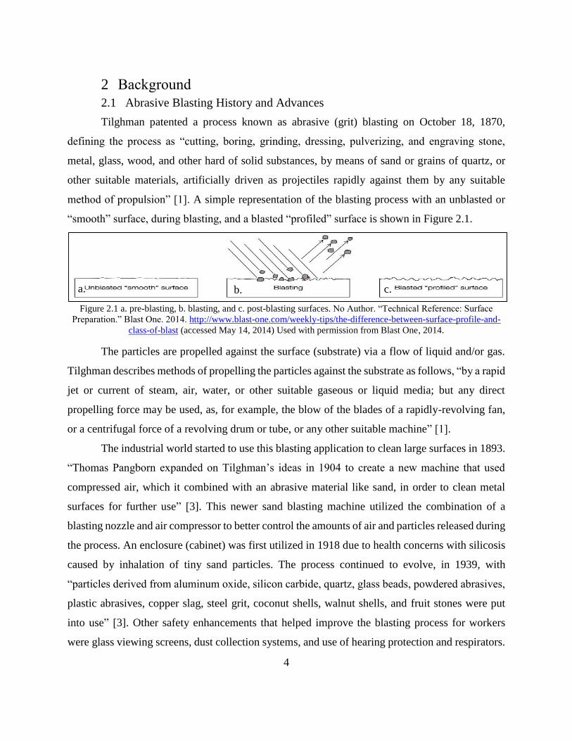
Tilghman patented a process known as abrasive (grit) blasting on October 18, 1870,

defining the process as “cutting, boring, grinding, dressing, pulverizing, and engraving stone,

metal, glass, wood, and other hard of solid substances, by means of sand or grains of quartz, or

other suitable materials, artificially driven as projectiles rapidly against them by any suitable

method of propulsion” [1]. A simple representation of the blasting process with an unblasted or

“smooth” surface, during blasting, and a blasted “profiled” surface is shown in Figure 2.1.

Figure 2.1 a. pre-blasting, b. blasting, and c. post-blasting surfaces. No Author. “Technical Reference: Surface

Preparation.” Blast One. 2014. http://www.blast-one.com/weekly-tips/the-difference-between-surface-profile-and-

class-of-blast (accessed May 14, 2014) Used with permission from Blast One, 2014.

The particles are propelled against the surface (substrate) via a flow of liquid and/or gas.

Tilghman describes methods of propelling the particles against the substrate as follows, “by a rapid

jet or current of steam, air, water, or other suitable gaseous or liquid media; but any direct

propelling force may be used, as, for example, the blow of the blades of a rapidly-revolving fan,

or a centrifugal force of a revolving drum or tube, or any other suitable machine” [1].

The industrial world started to use this blasting application to clean large surfaces in 1893.

“Thomas Pangborn expanded on Tilghman’s ideas in 1904 to create a new machine that used

compressed air, which it combined with an abrasive material like sand, in order to clean metal

surfaces for further use” [3]. This newer sand blasting machine utilized the combination of a

blasting nozzle and air compressor to better control the amounts of air and particles released during

the process. An enclosure (cabinet) was first utilized in 1918 due to health concerns with silicosis

caused by inhalation of tiny sand particles. The process continued to evolve, in 1939, with

“particles derived from aluminum oxide, silicon carbide, quartz, glass beads, powdered abrasives,

plastic abrasives, copper slag, steel grit, coconut shells, walnut shells, and fruit stones were put

into use” [3]. Other safety enhancements that helped improve the blasting process for workers

were glass viewing screens, dust collection systems, and use of hearing protection and respirators.

c. a. b.

5

Along with media selection and process safety improvements, the abrasive process was

eventually automated to produce better control of the process. In 1968, Progressive Engineering

Company built its first automated abrasive grit blasting system and by 1972, the company had

created its first pneumatic blasting product for the shot peening process [4]. The latest blasting

process improvement was the introduction of the robotic, ultra-high pressure water stripping

systems in 1992. Today, Wheelabrator (created with the help of Tilghman’s research and

invention) and Empire are two large blasting cabinet manufacturers that have become world

leaders in the abrasive blasting for the purposes of surface roughening, cleaning, material removal,

texturing, and deburring.

2.1.1 Various Blasting Methods

There are various types of abrasive blasting media propulsion systems currently used in

industry and research facilities. Table 2-1 includes a list of four types of blast cleaning methods,

specified by ISO 12944-4. Each type of blast cleaning will be reviewed, with an emphasis on dry

abrasive blast cleaning via compressed air.

Table 2-1 ISO 12944-4 Blast cleaning methods. Momber A. Blast Cleaning Technology: Chapter 1: Introduction,

2008. p. 3. http://link.springer.com/chapter/10.1007%2F978-3-540-73645-5_2 (accessed March 31, 2013) Used with

permission from Copyright Clearance Center, 2014.

Dry abrasive blast cleaning Centrifugal abrasive blast cleaning

Compressed-air abrasive blast cleaning

Vacuum or suction-head abrasive blast

cleaning

Moisture-injection abrasive blast

cleaning

(No further subdivision)

Wet abrasive blast cleaning Compressed-air wet abrasive blast

cleaning

Slurry blast cleaning

Pressurized-liquid blast cleaning

Particular applications of blast cleaning Sweep blast cleaning

Spot blast cleaning

Dry abrasive blasting is one of the most widely used blasting processes. The dry abrasive

blasting technology includes the use of compressed-air (pressurized), suction, and centrifugal

blasting media propulsion methods. Figure 2.2 shows an image of the design of the pressure and

suction blasting systems.

6

Figure 2.2 Suction and pressure blasting systems. No Author. “Blast Cabinets.” Norton Sandblasting Equipment,

2014. http://www.nortonsandblasting.com/nsbcontact.html (accessed May 14, 2014) Used with permission from

Norton Sandblasting Equipment, 2014.

In the pressurized blasting system, media is fed by gravity from a blast media pot into the

air line through an orifice at the bottom of the pot. Advantages of pressurized media blasting

include greater media velocity, quicker media mass flow, higher stand-off distance, and more

productive than suction systems [7].

Suction blasting operates via the venture principle to pull abrasive media from a non-

pressurized hopper to the blast nozzle at which it is combined with the compressed air stream and

propelled against a substrate [7]. Advantages of the suction blasting process include lower capital

equipment cost, easier maintenance, and less air and abrasive demand (lower energy cost).

2.1.2 Control Systems

Generally, the abrasive blasting process has three levels of control: manual, automatic, and

semi-automatic.

Manual systems entail blasting the substrate by moving the nozzle (and possibly hose

location) and media flow meter manually.

Fully automatic systems tend to control the location of the nozzle with respect to the

substrate, an automatic media flow regulation valve, and controls for the time or coverage

area of blasting.

Semi-automatic systems are often hybrids of manual and automatic systems, which could

include the computer aided control of the nozzle with a manual media flow regulation unit

or manual control of the nozzle with assistance from an automatic media flow regulator.

7

For small manual systems, the blasting operator utilizes the protected blast cabinet to

control the blast nozzle location via gloves. These cabinet systems are used for smaller substrates

and monitored from the protection viewing window. Disadvantages with the manual blasting

systems include the lack of accuracy of attack angle detection, no readout for stand-off distance,

uncontrolled or variable media flow rates that can alter, and no control of blasting time or coverage.

Some applications that require better control employ automatic basting systems. The use of an

automatic media flow regulator can allow for better media to air flow ratios and optimize the

blasting production rate. An automated nozzle controls along with programming, allow for: more

accurate blast angle, distance, blasting rate (step size and traverse rates), full blasting time, and

area coverage.

The abrasive blasting process can be fine-tuned and adjusted to create better results, save

time, and improve the process yield. Unfortunately, some substrates are larger than a blast cabinet

or blast room can accommodate and have to be blasted manually due to their size and possibly

blasted on location. Manual blasting is more versatile in some scenarios and performed in smaller

blasting locations or to blast uniquely shaped substrates with ease.

Semi-automated blasting units comprise both manual and automated blasting systems. This

type of system could have the advantages of blasting in any environment, along with the ability

for better control of the nozzle and media flow. Fixtures can be used to control the blast distance

or angle, while the pressure is controlled via an automatic media flow regulator. Blast time can be

controlled automatically, while still having the versatility of moving the nozzle at different angles

to generate desired results. Another improvement would be to use a laser system to help monitor

the nozzle distance from the substrate.

2.2 Abrasive Media

Different properties of the abrasive media play a role in material selection for blasting

processes. Some of these properties are media shape, size, hardness, density, type, fracture

strength, and presence of impurities. All of these mentioned properties or qualities will be

discussed in the following section.

2.2.1 Abrasive Shape

The blasting media shape can be separated into different categories: round, irregular,

globular, or cylindrical. Each shape of media can further defined by properties such as shape

8

factor, circularity factor, roundness, sphericity, elongation ratio, and flatness ratio. Equations for

each of those properties are listed below. Figure 2.3 shows the diagrams for the determination of

the six media shape definitions mentioned above.

Shape Factor 𝐹𝑠ℎ𝑎𝑝𝑒 =𝑑𝑚𝑖𝑛

𝑑𝑚𝑎𝑥 (1)

Circulator Factor 𝐹0 =4∙𝜋∙𝐴𝑝

𝑃𝑒𝑟𝑖𝑚𝑒𝑡𝑒𝑟2 (2)

Roundness 𝑆𝑅 =∑

2∙𝑟𝑐𝑜𝑟𝑛𝑒𝑟𝑑𝑃

𝑁𝑐𝑜𝑟𝑛𝑒𝑟 (3)

Sphericity 𝑆𝑃 =√

4

𝜋∙𝑏𝑃∙𝑙𝑝

𝑁𝑐𝑜𝑟𝑛𝑒𝑟 (4)

Elongation ratio 𝑟𝐸 =𝑙𝑃

𝑏𝑃 (5)

Flatness ratio 𝑟𝐹 =𝑙𝑃

𝑡𝑃 (6)

Figure 2.3 Media shape definitions; a. shape factor & circulatory factor, b. roundness, & sphericity, & c. elongation

ratio & flatness ratio. Momber A. Blast Cleaning Technology: Chapter 2: Abrasive Materials, 2008. p. 19.

http://link.springer.com/chapter/10.1007%2F978-3-540-73645-5_2 (accessed March 31, 2013) Used with

permission from Copyright Clearance Center, 2014.

The particle shape can also be defined by the geometrical form, and the relative proportions

of length, breadth, and thickness [8]. Shape factor, circularity factor, roundness and sphericity all

refer to the geometrical form of the media. The shape factor is defined as the ratio of the small

diameter particle (dmin) to the large diameter (dmax) particle [8, 9]. This simply means that as the

c. a. b.

9

shape factor approaches unity, the particle is more spherical. The circularity factor takes the

particle area and the particle perimeter into account. As the circularity factor approaches unity, a

particle of spherical shape occurs similar to the shape factor. Gillepsie and Fowler showed that a

circularity factor of F0 > 0.83 classified a particle as shot media. As the circularity and shape factor

values decrease, the particles become less spherical and more angular in shape.

The roundness of a particle can be defined as the sum of the corner diameter-core diameter

ratio divided by the number of corners. A “round” particle has less corners or edges present, while

a tetragonal would have four corners. The particle sphericity suggested by Wadell (1933) was

determined by particle length and breadth (width), along with the diameter of a circle that the particle

edges will touch, but not pass over [10]. Figure 2.4a shows another roundness scale, developed by

Hansink, which defines particles as angular or round. Figure 2.4b demonstrates a relationship between

sphericity and roundness. Particles can be round, spherical, a combination of both, or neither based on

this roundness and sphericity chart.

Figure 2.4 a. Hansink’s shape designations & b. garnet roundness-sphericity chart. Momber A. Blast Cleaning

Technology: Chapter 2: Abrasive Materials, 2008. p. 21. http://link.springer.com/ chapter/10.1007%2F978-3-540-

73645-5_2 (accessed March 31, 2013) Used with permission from Copyright Clearance Center, 2014.

Bahaduur and Badruddin created the ratios for the purpose of determining the influence of

abrasive particle shape on particle erosion processes [13]. The particle length to particle breadth

ratio is the elongation ratio and the flatness ratio is the ratio of particle length to particle thickness.

In either case, the particle is considered to be elongated or flat with a decrease of this value. A

relationship between particle shape, type, and diameter is shown in Figure 2.5.

a. b.

10

Figure 2.5 Shape, size, and type relationships. Momber A. Blast Cleaning Technology: Chapter 2: Abrasive

Materials, 2008. p. 20. http://link.springer.com/chapter/10.1007%2F978-3-540-73645-5_2 (accessed March 31,

2013) Used with permission from Copyright Clearance Center, 2014.

2.2.2 Grit, Shot and Cylindrical

“The term grit characterizes grains with predominantly angular shape and they exhibit

sharp edges and broken sections” [14]. Grit is typically classified by the shape parameters

mentioned previously. A particle can be classified as grit if the shape factor, F0, is under 0.8 and

has a sphericity above 0.6 and roundness above 0 or a roundness from 0 to 0.25 and sphericity of

0.4 as shown in Figure 2.4b. Figure 2.6 shows an image that compares grit media (top) and shot

media (bottom) [15].

Figure 2.6 a. Grit image and b. shot image. Momber A. Blast Cleaning Technology: Chapter 2: Abrasive Materials,

2008. p. 18. http://link.springer.com/chapter/10.1007%2F978-3-540-73645-5_2 (accessed March 31, 2013) Used

with permission from Copyright Clearance Center, 2014.

Because of its angular shape, grit media is used for several purposes.

Surface roughening - roughen for polymeric coatings that need adhesion to substrates.

b.

a.

11

Material Removal - remove rust, scale, or any unwanted debris to clean a substrate. Grit

can also be utilized to remove mass from a product to reduce its weight for various

applications.

Texturing - grit media is used to create a certain luster or aesthetic appearance [16].

Detailing- micromachining or micro blasting to create intricate details or machine uniquely

shaped substrates.

Another shape designation is known as shot media, which generally is used in the shot

peening process. “The term shot characterizes grains with a predominantly spherical shape. Their

length-to-diameter is < 2, and they do not exhibit sharp edges or broken sections” [14]. The shape

factor for shot media is F0 > 0.8. As the four geometrical form shape parameters approach unity,

the shot media becomes more spherical. Shot media is typically used to generate a compressive

stress layer on the substrate. Upon shot peening of the machined part, a continuous compressive

stress layer covers the surface. “The compressive layer stops the fatigue cracks and stress corrosion

that typically start at the surface of the part” [17].

The last media shape used for blasting is known as cylindrical media. “The term cylindrical

denotes grains that are manufactured by a cutting process and their length-to-diameter ratio is ~1”

[14]. A simple example of a cylindrical shaped particle is corn cob media.

2.2.3 Abrasive Size & Size Distribution

The size of the abrasive grits is another factor that determines the effect of the blasting

process. “Coarse grains are measured in inches or millimeters, fine particles in terms of screen

size, and very fine particles are measured in micrometers or nanometers” [14]. These descriptions

are based on the average particle diameters for a certain size distribution of particles, which can

be determined through several calculations. One example for calculating the size distribution of

media is shown as follows [14]:

𝑀0(𝑑𝑝) = 𝑓((𝑑𝑝)

(𝑑∗))𝑛𝑀 (7)

M0 is the particle size distribution function, where the particle diameter is defined as (dp),

average particle diameter (d*), and measure of the particle size spread (nM). “The higher the

value for nM, the more homogeneous is the grain size structure of the sample. For nM → ∞, the

sample consists of grains with equal diameters” [14]. To generate a uniform and repeatable blasted

surface, the size distribution needs to be small.

12

SSPC-AB standards and SAE standards define the size distribution from a percentage of

weights from specific sets of sieves. In the sieve analysis method, the particles are displaced on

the top of the sieve system, which has different sieve meshes stacked vertically. The screen

openings of each sieve become smaller as the media approaches the bottom sieves. Each sieve is

then emptied out and weighed to calculate the amount of particles in each section, which will be

the different sizes of the particles. Figure 2.7 shows the size distribution of alumina 700 and

Metagrit 65 after using this sieving method. The alumina particles have a bell-curve shaped size

distribution and the Metagrit has a skewed bell-curve distribution.

Figure 2.7 Distribution of sieve analysis. Momber A. Blast Cleaning Technology: Chapter 2: Abrasive Materials,

2008. p. 26. http://link.springer.com/chapter/10.1007%2F978-3-540-73645-5_2 (accessed March 31, 2013) Used

with permission from Copyright Clearance Center, 2014.

Four methods used to define media size are:

Particle diameter - the average particle size diameter is calculated for a known particle size

distribution.

Sieve size - designates the particles into the different size sieves or mesh sizes. Sigma-

Aldrich displays this relationship of the mesh designation and nominal sieve openings in

table format [19].

Mesh size - the mesh number increases, the particle size and sieve openings decrease and

is correlated with the meshes present in the sieving process. The following equation can be

used to calculate average particle size from the mesh size [20]:

𝑑𝑝 = 17,479 ∙ 𝑚𝑒𝑠ℎ−1.0315 (8)

13

Grit size -Sometimes media are categorized based on grit size, instead of meshes, which

manes “the number of standardizes holes that fit within the standard dimensional sized

scree, i.e., 200 holes equals 200 grit” [21]. Newport Glass Works, LTD shows the

correlation between grit size designation and the average, maximum, and minimum particle

sizes in another table. Additionally, Media Blast & Abrasive, Inc. has similar information,

with the addition of the USS mesh sizes [22].

The particle size will have a tangible effect on the blasting performance. Smaller grit

particles tend to yield rougher surfaces and less surface contamination and higher surface

roughness, while medium particles result in the most surface contamination as shown in Figure

2.8.

Figure 2.8 Grit contamination vs. roughness. Day, James; Huang, Xiao; and Richards, N.L. “Examination of a Grit-

Blasting Process for Thermal Spraying Using Statistical Methods.” Journal of Thermal Spray Technology,

2005/Vol. 14, p. 477. http://link.springer.com/article/10.1361%2F105996305X76469 (accessed November 2012)

Used with permission from Copyright Clearance Center, 2014.

In another study, white alumina particles were blasted unto cold-rolled carbon steel. As the

grit size increases, the residual grit weight increases exponentially and the penetration depth

increases linearly. These findings are shown graphically in Figure 2.9. A separate study found a

correlation between grit size and substrate surface energy. The surface energy imparted unto the

substrate has been shown to have an inverse relationship with the grit size [25].

14

Figure 2.9 Grit diameter vs. a. residual grit and b. penetration depth. Maruyama T, Akagi K, Kobayashi T. "Effects

of Blasting Parameters on Removability of Residual Grit." Journal of Thermal Spray Technology. 2006/Vol. 15, no.

4. p. 820. http://link.springer.com/article/10.1361%2F105996306X147018 (accessed November 2, 2012) Used with

permission from Copyright Clearance Center; letter attached.

2.2.4 Abrasive Hardness

The hardness of the abrasive media is one of the main determining factors of which type

of media is selected for the abrasive blasting process. Material hardness can be defined as “the

property of matter described as the resistances of a substrate to being scratched by another

substance” [26]. When the media is significantly softer than the substrate, the surface will not be

properly smoothed, roughened, or cleaned. Conversely, media may inadvertently damage the

substrate when the substrate is much softer than the media.

Three common types of hardness testing methods for materials are scratching, indentation,

and penetration. The Mohs hardness scale is utilized for the scratching test and is shown is Table

2-2.

Table 2-2 Mohs hardness scale. Momber A. Blast Cleaning Technology: Chapter 2: Abrasive Materials, 2008. p.

14. http://link.springer.com/chapter/10.1007%2F978-3-540-73645-5_2 (accessed April 1, 2013) Used with

permission from Copyright Clearance Center, 2014.

Material Mohs Hardness

Talc 1

Gypsum 2

Calcite 3

Fluorite 4

Apatite 5

Orthoclase (Feldspar) 6

Quartz 7

Topaz 8

Corundum 9

Diamond 10

a. b.

15

For media hardness, the material is scratched by different materials shown in the table until it

cannot be scratched anymore. As an example, if topaz does not scratch the material, but corundum

scratches it, then the media would have a Mohs hardness of 8.5 [27].

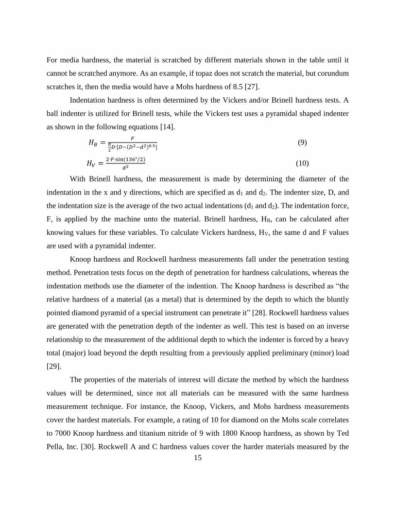
Indentation hardness is often determined by the Vickers and/or Brinell hardness tests. A

ball indenter is utilized for Brinell tests, while the Vickers test uses a pyramidal shaped indenter

as shown in the following equations [14].

𝐻𝐵 =𝐹

𝜋

2𝐷∙[𝐷−(𝐷2−𝑑2)0.5]

(9)

𝐻𝑉 =2∙𝐹∙sin(136°/2)

𝑑2 (10)

With Brinell hardness, the measurement is made by determining the diameter of the

indentation in the x and y directions, which are specified as d1 and d2. The indenter size, D, and

the indentation size is the average of the two actual indentations (d1 and d2). The indentation force,

F, is applied by the machine unto the material. Brinell hardness, HB, can be calculated after

knowing values for these variables. To calculate Vickers hardness, HV, the same d and F values

are used with a pyramidal indenter.

Knoop hardness and Rockwell hardness measurements fall under the penetration testing

method. Penetration tests focus on the depth of penetration for hardness calculations, whereas the

indentation methods use the diameter of the indention. The Knoop hardness is described as “the

relative hardness of a material (as a metal) that is determined by the depth to which the bluntly

pointed diamond pyramid of a special instrument can penetrate it” [28]. Rockwell hardness values

are generated with the penetration depth of the indenter as well. This test is based on an inverse

relationship to the measurement of the additional depth to which the indenter is forced by a heavy

total (major) load beyond the depth resulting from a previously applied preliminary (minor) load

[29].

The properties of the materials of interest will dictate the method by which the hardness

values will be determined, since not all materials can be measured with the same hardness

measurement technique. For instance, the Knoop, Vickers, and Mohs hardness measurements

cover the hardest materials. For example, a rating of 10 for diamond on the Mohs scale correlates

to 7000 Knoop hardness and titanium nitride of 9 with 1800 Knoop hardness, as shown by Ted

Pella, Inc. [30]. Rockwell A and C hardness values cover the harder materials measured by the

16

Vickers method and Brinell hardness covers the soft to medium hardness materials. The Vickers

hardness measurement range is the most applicable, since it umbrellas the entire spectrum of the

other hardness measurement types. More hardness value conversions can be seen in a table created

by NDT Resource Center [31].

Media selection will be based on the application and the substrate to be blasted. Equation

13 below shows the relationship of the media hardness to substrate hardness [32, 33].

𝐻𝑀

𝐻𝑃→ 1.0 𝑡𝑜 1.5 (11)

HM is the substrate hardness and HP is the hardness of the particle. An increase in abrasive specific

mass loss occurred with a ratio of HM/HP = 0.9 or lower as shown in Figure 2.10. For all three

substrate/media combinations, mass loss amounts increased with the increasing media hardness

levels. However when the ratio of 2.4 occurs, the function exhibited a steep decrease, so the media

hardness becomes obsolete at very high hardness values. Appendix A contains hardness values for

various media types [35].

Figure 2.10 Abrasive hardness effect on specific mass loss. Momber A. Blast Cleaning Technology: Chapter 2:

Abrasive Materials, 2008. p. 11, 12. http://link.springer.com/chapter/10.1007%2F978-3-540-73645-5_2 (accessed

March 31, 2013) Used with permission from Copyright Clearance Center, 2014.

2.2.5 Abrasive Density

Particle density can be important in terms of blasting pressure and media flow rates.

Particles with less porosity (higher density) affect the surface more than highly porous particles.

The apparent density (ρP) is shown below in Equation 14 where particle mass (mp) is related to

particle volume (vp) in terms of the particle diameter (dp) [14].

17

𝜌𝑃 =𝑚𝑃

𝑉𝑃=

6∙𝑚𝑃

𝜋∙𝑑𝑃3 (12)

This density parameter includes flaws, pores, and cracks [14]. The highly dense materials

generally have lower vacancies, while a material of low density would have many pores, cracks,

or flaws, which lower the particle mass. The particle density and apparent density terms are

synonymous, since they include material mass and the mass of void space in the particles. Bulk

density would refer to the mass of the media in relation to its volume, only including the amount

of the material, excluding effects of pores, flaws, and cracks.

2.2.6 Type (Metallic vs. Non-Metallic)

Blasting media can also be categorized into metallic and non-metallic abrasives. Cost,

substrate type, and environmental effects play a role in which type of media is chosen for a

particular application as well. Some common metal abrasives are iron grit, copper slag, and steel

grit/shot. The difference in steel grit and shot is that the grit would remove more substrate mass,

whereas the shot would just peen the surface more. Figure 2.11 displays images of steel shot and

steel grit on the left and brown corundum and demetalized steel slag on the right [36].

Figure 2.11 a. Steel shot, b. steel grit, c. brown corundum, & d. demetalized steel slag. Makova, I., Sopko, M.

"Effect of Blasting Material on Surface Morphology of Steel Sheets." Acta Metallurgica Slovaca. 2010/ Vol. 16, no.

2, p. 111. (accessed March 07, 2013) Used with permission from Acta Metallurgica Slovaca, 2014.

Non-metallic materials encompass many different types of elements, compounds, or

composites, but ceramic media is most commonly found in the grit blasting industry. White, pink,

and brown alumina, garnet, coal slag, silica sand, quartz, and corundum are some non-metallic

media used in industry, while glass beads and plastic falling under the shot category as shown in

Appendix A. Ceramic bead media might be selected for applications which require high life cycles

a

. b. c

.

d.

18

(60-100) and low dust debris, and cost is not the primary factor. Coal slag is often utilized because

of its low cost, but it has a life cycle of one use and high amounts of dust debris. Garnet has low

dust accumulation, medium cost, and 3-4 uses before it becomes ineffective and aluminum oxide

has low dust debris, 6-8 cycles, and a relatively high cost. Media types (including silica) that

generate a high amount of dust should be blasted in a contained environment and breathing

equipment should be used by operators.

2.2.7 Fracture Strength

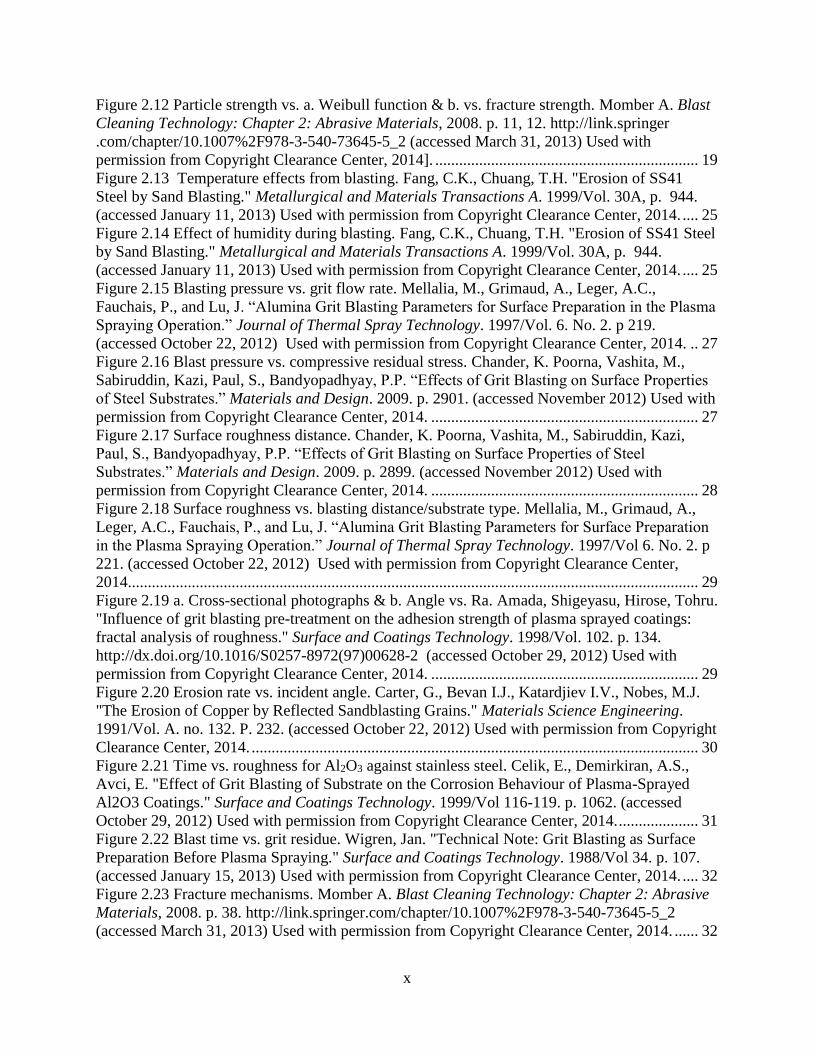
Fracture strength is “the minimum tensile stress that will cause fracture” [37]. This tensile

stress is of force (tension) applied to a cross-sectional area of a given material. Typically, the media

fractures due to wear over repeated recycling during the blasting process. In some cases, media

replacement is necessary other times the media breaks down due to manufacturing defects “such

as micro-cracks, interfaces, inclusions, or voids” [14]. Huang applied the Weibull distribution to

abrasive materials. Equation 13 shows a simple equation for particle fracture strength (σF), and its

relationship with particle volume (Vp), defect distribution strength parameter (σ*), and Weibull

modulus (mw) [38].

𝐹(𝜎𝐹) = 1 − exp [−𝑉𝑃 ∙ (𝜎𝐹

𝜎∗)𝑚𝑤] (13)

For this equation, mw determines if the variability of particle strength among a given set of

particles is high or low. When mw is low, the variability in particle strength of those particles would

be high. Figure 2.12a shows the Weibull modulus plotted against the particle strength and the

deviation from the trend line represents variation. Figure 2.12b shows the fracture strength

decreases as corundum particles increase in size. Based on these two graphs, scatter in strength of

abrasive particles is shown to be wider for larger particles [14].

19

Figure 2.12 Particle strength vs. a. Weibull function & b. vs. fracture strength. Momber A. Blast Cleaning

Technology: Chapter 2: Abrasive Materials, 2008. p. 11, 12. http://link.springer .com/chapter/10.1007%2F978-3-

540-73645-5_2 (accessed March 31, 2013) Used with permission from Copyright Clearance Center, 2014].

The quality of the grit is important to the surface quality of when blasting the substrate.

For instance, ISO 11124/2-4 is one example that sets maximum limits for the following particle

properties by %: particle shape change, number of voids, shrinkage defects, cracks, and total defect

% for chilled iron grit, high-carbon cast steel shot and grit, and low-carbon cast steel shot [40].

2.2.8 Impurities

The probability of the incorporation of impurities into the blasting media is relatively

difficult to predict, but contamination can originate from the substrate, blast cabinet, and work

environment. Solid and liquid impurities such as dust, lead, water soluble contaminants, and oil

can be present in a media storage container. Accidental mixing of different media can occur

when switching out media between blasting operations. Some solid foreign particles can be detected

via magnetization or visual inspection. Impurity limitations can be set for recycled media and may

include non-abrasive residue, lead content, water soluble contaminants, and oil content [41].

Conductivity testing and/or chemical analyses are other methods used to detect soluble foreign

matter.

2.3 Substrates

For the abrasive blasting process, the substrate can be a deciding factor in which process

parameters, media selection, and blasting machines are used to create a desired surface roughness,

texture, thickness or mass removal amount. Some typical properties of substrates that are taken

into consideration are substrate hardness, thickness, strength, and initial surface roughness. Other

a. b.

20

properties such as substrate shape, pre-blasting strains and/or stresses, and cleanliness are

important as well.

2.3.1 Substrate Material

Three generic types of substrates are blasted: metals, polymers, or ceramics. These

substrate material are generally based on application, thus media selection occurs based on desired

substrate surface modification.

Metals are classified as materials that are composed of one or more metallic elements (such

as iron, aluminum, copper, titanium, gold, etc.) and nonmetallic elements (carbon, nitrogen,

oxygen, etc.) in relatively small amounts [42]. Metals have a higher density than other materials,

including composites, and have the highest tensile strengths as well. Metals are very stiff and have

superb fracture toughness values. For ductile metals, sodium bicarbonate, plastic media, and

walnut shells are commonly used to remove substrate mass. Media that are not spherical should

be utilized on metals that need to be roughened and aluminum oxide is often used for removing

mass and roughening harder, brittle substrates.

Polymer substrates are difficult to blast due to their unique properties. These materials

consist of carbon backbones with hydrogen, oxygen, nitrogen, and silicon forming organic

compounds with large molecular structures. Polymers have lower densities, tensile strengths, and

fracture toughness values than metals and ceramics. As mentioned previously, beads or shot are

optimum media to use based on polymers being very flexible and not hard. One drawback of

polymer substrates is the need to keep the substrate in a narrow temperature range to reduce

changes of degradation. With this in mind, polymers need to be blasted under conditions that would

roughen the surface or remove mass, not destroy the entire substrate or melt the substrate due to

over blasting.

Ceramic materials mainly consist of oxides, nitrides, and carbides [42]. Ceramic substrates

are extremely hard, brittle, and can withstand higher temperatures than polymers and metals. High

tensile strengths, high stiffness, and low fracture toughness values are given for ceramics. Due to

the brittle nature of ceramics, very hard media needs to be applied when blasting ceramic

substrates, given that the substrates are thick enough not to be blasted through easily. Typically,

ceramic materials are used as media in the blasting operations, but in some cases, ceramics can be

the substrate due to customer specifications.

21

2.3.2 Substrate Hardness

Substrate hardness can determine which type of media is best to use based on “hardness

interactions” as shown in Equation 11. Substrate or stock hardness can indicate how much abrasive

velocity is required to clean or roughen the surface and how much stock is removed from blasting.

Softer materials might absorb the media energy and burn the substrate if the wrong blasting

parameters or wrong type of media are used while blasting. Harder substrates are easier to blast

without the worry of media energy/heat absorption, however an increase in media velocity is

needed to roughen, clean, or remove mass from those substrates. Typically, blasting angle is varied

for substrates based on their different hardness too.

2.3.3 Substrate Thickness

The specimen thickness can play various roles in the effectiveness of the grit blasting

process. Thick substrates are less likely to deform due to the amount of bulk substrate material,

whereas thinner substrates could break or bend due to blasting at the high pressures or close

distances from the substrate. Figure 13 found in “Residual Stress on the Grit Blasted Surface” by

Tosha and Iida shows that thinner substrates have more susceptibility to surface residual stresses

and once a thickness of 4 mm is reached, the surface residual stress value becomes constant at -

200 MPa for grit blasting [43]. Shot peening created more residual surface stresses as expected

and peaked out at 6 mm thickness. Tosha and Iida also suggested that when the work hardened

layer and substrate thickness overlap, the surface residual stress is zero [43].

2.3.4 Substrate Shape

Pre-blasted substrate shape can have an effect on the blasting process used. For instance a

pyramid, cube, or cylinder substrates would have to be blasted in different patterns. As one would

expect, a cube is simple to blast, just making sure to spend the same amount of time blasting on

each face of the cube. A pyramid shaped substrate would have to be blasted in a similar fashion,

with more consideration of the blast radius, traverse rate, and step sizes, which will be discussed

under the process parameters section. Any of these substrate shapes, especially the sphere or

cylindrical shape, could be blasted by having a rotating platform that keeps the substrates spinning

around the z-axis, while the nozzle just moves in the x or y and z directions. The shape of the

substrate can also effect the angle at which the substrate needs to be blasted and for unique not

22

geometrical substrates, problems like over-blasting, heat generation, and coverage would be

primary issues to be considered before blasting.

2.3.5 Initial Surface Roughness

One purpose of surface roughness altering is “extending the surface area of the substrate

allowing an adhesive or coating to flow in or on them” [44]. The initial roughness of the substrate

can be defined as a smooth or rough surface in terms of numerous roughness qualities. Although

it takes more time to blast a smooth surface, it tends to have less residual grit and grit reflection

can be more controlled. The blast zone is harder to predict on a rough surface so grit reflection and

surface uniformity would be harder to control.

A simple understanding of some of the many roughness parameters gives insight to what

roughness actually means quantitatively. ISO reports surface structure under three different

categories: primary profile (P), roughness profile (R), and waviness (W). Ra is the arithmetic-mean

deviation of the assessed profile [45]. Some other parameters in Bacova and Draganovska’s study

were Rq, Rt, Rv, Rz, Rc, SSm, and RPc. Rq is the root-mean square, Rt is described as the total height

of the profile over a given length, RP is the maximum peak height and Rv is the maximum peak

depth. Rpc is the density of peaks for a profile, which corresponds to the number of peaks per

profile unit length [45]. Rz is the maximum height or highest peak, of the profile, the mean height

of the profile peaks is termed Rc, and RSm is used to describe the mean peak width for a given

profile. Rsk is the profile skewness, while Rku is the roughness kurtosis, and Rz represents the ten

point height testing method. Equations for Ra, Rq, Rz, Rt, Rsk, and Rku are shown below [46].

𝑅𝑎 =1

𝑛∑ 𝑆𝑖

𝑛𝑖=1 (14)

𝑅𝑞 = √1

𝑛∑ 𝑆𝑖

2𝑛𝑖=1 (15)

𝑅𝑧 =∑ 𝑠𝑝𝑖−∑ 𝑠𝑣𝑖

𝑠𝑖=1

𝑠𝑖=1

𝑆 (16)

𝑅𝑡 = 𝑚𝑎𝑥𝑖𝑠𝑖 − 𝑚𝑖𝑛𝑖𝑠𝑖 (17)

𝑅𝑠𝑘 =1

𝑛𝑅𝑞3 ∑ 𝑆𝑖

3𝑛𝑖=1 (18)

𝑅𝑘𝑢 =1

𝑛𝑅𝑞4 ∑ 𝑆𝑖

4𝑛𝑖=1 (19)

23

2.3.6 Pre-Blasting Strains and Stresses

Normally, it is assumed that substrates for the abrasive blasting operation are under

negligible strain (especially if the substrate isn’t attached or part of a load-bearing application).

The effects of the blasting media and parameters will contribute to the stress and strain changes.

In real world applications, pre-strained substrates would be expected if a substrate was part of a

machine or structure and was blasted in an open environment while being pre-strained during or

prior to blasting.

A study by Tosha and Iida looked at the effects of pre-strain on 304 austenitic stainless

steel substrates [47]. Pre-strain occurred at 0%, 10%, 20%, and 35% prior to blasting and the effect

of work-softening occurred on the substrates. Generally, when grit blasting a work-hardened layer

would be present after blasting. Due to the pre-strain that occurred prior to blasting, the opposite,

work softening was noticed for all substrates with the pre-strain applied before blasting. One set

of experiments used steel shot, while the other used steel grit. The effects of the grit blasting

softening effect on the pre-strained substrates was more pronounced with a maximum softening

ratio of 8.3% from blasting [47].

2.3.7 Cleanliness

Contamination evaluation must occur based on the type of contaminant, amount of

contaminant, depth of contamination layer, and friability of contaminant. Common examples of

surface contamination are excess oil, lubricants, dust, water, organic, and inorganic materials.

External contaminants are materials or debris that appear on the substrate due to the surrounding

environment or finishing part processes. Examples of human sources are finger prints, cigarette

smoke, drink residues, and mucous, while non-human error environmental contaminants are

lubricating oils and silicone greases.

Different types of contamination effect the surface properties of the substrates as shown in

the Handbook on Adhesion Technology. In most cases, adhesive strength is evaluated for purposes

of future coatings, however, in blasting operations, adhesives are also used as masking materials

to protect parts of the substrate from being blasted. Thus, knowing how contamination effects

adhesion to a substrate before and after blasting is relevant. Smith and Crane performed a study

on the influence of contamination levels on adhesive strength of aluminum alloy adherents, with

lubricating oil and silicon grease being contamination sources [48]. An increase in water contact

24

angle to 100° occurred when high levels of lubricating oil were added to a surface, while small

levels, 3.5 to 20 nm, of silicone grease led to increases in the water contact angle and a huge

reduction in failure load [44]. Another study, by Minford, demonstrated the effect of emulsified

lubricants on 2036 T4 aluminum [49]. The joint strength of the aluminum lap-shear joint regions

began to decrease at 0.82 mg/cm2 of oil and after 0.95 mg/cm2 of oil, the strength decreased from

10 to 6 MPa, and the level of cohesiveness decreased as well.

A few methods of degreasing metal adherents or substrates are simple immersion, wiping

techniques, vapor degreasing, ultrasonic cleaning, etching, grit blasting, and surface temperature

treatments. Environmentally safe alternatives are detergent degreasing and alkaline cleaners.

Recommended methods for polymer contamination removal are flame treatment, corona discharge

treatment, and plasma treatment [44]. For composites, the two best surface contamination

reduction methods are peel plies, which are sacrificial external surface layers, and the use of

surface abrasion (grit blasting) to eliminate the contaminated layer. Contamination lowers surface

energy, which is related to the surface roughness and adhesion strength of substrates.

2.4 Blasting Environment

During the blasting process, both cabinet temperature and humidity can play a role in the

outcomes seen from blasting [50]. The temperature of the blasting process is generally ambient or

room temperature, but can vary based on the different blasting operations/locations. Humidity is

generally location specific, but results will vary if blasting on a factory floor versus outside in ship

hull blasting. “Little research has been done on the effect of temperature on erosion damage, while

research on the influence of humidity on erosion could hardly be found in the literature” [50].

2.4.1 Temperature

Fang and Chuang showed that as substrate temperature increases, erosion loss or stock

removal decrease for aluminum, stainless steel, and a titanium alloy [50]. Another one of their

studies suggests that erosion damage might be varied with change in blast (attack) angle. Figure

2.13 displays these results for SS41 steel temperature and blast angle effects on volume loss, worn

area, and mean penetration depth.

25

Figure 2.13 Temperature effects from blasting. Fang, C.K., Chuang, T.H. "Erosion of SS41 Steel by Sand Blasting."

Metallurgical and Materials Transactions A. 1999/Vol. 30A, p. 944. (accessed January 11, 2013) Used with

permission from Copyright Clearance Center, 2014.

The blast temperature of 45oC led to the least amount of volume loss/stock removal,

smallest amount of worn area, and largest scar depth. For volume loss, lower temperatures led to

more volume loss, suggesting that an elevated temperature might help save substrate stock in

surface texturing applications. Certain substrate temperatures lead to a minimizing effect on mean

depth of scars. Blast angle had an effect on these results as well.

2.4.2 Humidity

The effects of humid blasting environments have been of little discussion by research

groups, although Fang and Chuang also studied blasting angle variation with four different

humidity levels. Figure 2.14 displays the results of their studies with emphasis on 50, 65, 80, and

95% relative humidity.

Figure 2.14 Effect of humidity during blasting. Fang, C.K., Chuang, T.H. "Erosion of SS41 Steel by Sand Blasting."

Metallurgical and Materials Transactions A. 1999/Vol. 30A, p. 944. (accessed January 11, 2013) Used with

permission from Copyright Clearance Center, 2014.

a. b. c.

b. c. a.

26

Some effects are noticeable regardless of blasting angle, which are that 80% RH led to the most

volume loss and worn area, while 65% RH generated the smallest mean scar depths. Most of the

data shown suggests that attack angle and humidity have a combination effect on surfaces, except

that when attack angle increases, the mean depth decreases in most cases.

2.5 Blasting Process Parameters

There are many important factors that lead to changes in surface modification from grit

blasting. Some of these process factors are: blasting pressure, stand-off distance, attack angle, blast

time, coverage, media size degradation over time, media flow rate, media velocity, media impact

energy, etc. The blasting pressure effects the media flow rate, media and air velocity, and to a

certain extent the blast pattern generated. Assuming that the media flow is completely straight (no

curvature due to low flow rate), the blast angle is the angle between the substrate and the media

stream exiting the nozzle or the nozzle itself. . Stand-off distance is the direct distance from nozzle

exit (possibly nozzle throat) to the substrate during blasting. Media flow or mass flow rate is

effected by the amount and size of media, blasting (air) pressure, air velocity/volume, and blasting

hose dimensions.

2.5.1 Blasting Pressure and Media Flow Rate

In any kind of dry abrasive blasting system, compressed air or gas is used to propel the

media through a nozzle and unto the substrate. The amount of media leaving the nozzle and hitting

the substrate (media flow/mass flow rate) and particle velocity are affected by the compressed air

pressure. When the blast nozzle geometry stays constant and the hose and media flow regulator

are not obstructed by various objects, the increasing blast pressure leads to higher abrasive flow

and abrasive velocities. Figure 2.15 shows the effect of blasting pressure on grit blast rate (kg/min).

As the blasting pressure increases, the grit flow rate increased regardless of grit size. A similar

effect can be noted if the nozzle opening becomes smaller and the same blast pressure is used.

27

Figure 2.15 Blasting pressure vs. grit flow rate. Mellalia, M., Grimaud, A., Leger, A.C., Fauchais, P., and Lu, J.

“Alumina Grit Blasting Parameters for Surface Preparation in the Plasma Spraying Operation.” Journal of Thermal

Spray Technology. 1997/Vol. 6. No. 2. p 219. (accessed October 22, 2012) Used with permission from Copyright

Clearance Center, 2014.

Roughness, adhesion strength, and residual stress are found to be related to pressure

changes. Another study by Tosha and Iida shows that both grit and shot on stainless steel and

titanium substrates generate higher Rmax values, with grit roughening the surface more than shot,

as expected [52]. The magnitude of residual stresses generated from blasting low carbon steel with

alumina grit are shown in Figure 2.16. An increase in blast angle led to more compressive residual

stresses, as did an increase in blast pressures for all three angles.

Figure 2.16 Blast pressure vs. compressive residual stress. Chander, K. Poorna, Vashita, M., Sabiruddin, Kazi, Paul,

S., Bandyopadhyay, P.P. “Effects of Grit Blasting on Surface Properties of Steel Substrates.” Materials and Design.

2009. p. 2901. (accessed November 2012) Used with permission from Copyright Clearance Center, 2014.

2.5.2 Stand-off Distance

Blasting or standoff distance is the exact distance between the blasting nozzle and the

substrate specimen and is usually listed in units of centimeters (cm), millimeters (mm), or inches

28

(in). If the distance is very small, then blasting might roughen the surface too much in localized

zones, but if the distance is too far, media velocity would decrease and the substrate would barely

be eroded, scarred, or grazed, if at all. Figure 2.17 displays a similar effect when alumina was

blasted on steel substrates at different distances. At a blast distance of 100 mm, the maximum

roughness was obtained and distances shorter or further seemed to create smaller increases in

surface roughness.

Figure 2.17 Surface roughness distance. Chander, K. Poorna, Vashita, M., Sabiruddin, Kazi, Paul, S.,

Bandyopadhyay, P.P. “Effects of Grit Blasting on Surface Properties of Steel Substrates.” Materials and Design.

2009. p. 2899. (accessed November 2012) Used with permission from Copyright Clearance Center, 2014.

Figure 2.18 links blast distance, grit size, and substrate type into one set of results. This

figure shows “that, for a given material, Ra increases with the blasting distance, d, up to 100 mm,

remains almost constant up to 150 mm, and then decreases again for higher values of d” [51].

However, each substrate had different roughness values at the various blasting distances. The

aluminum was roughened the most up to this 100 mm distance, with FT25 being next, and 100C6

being roughened the least for all three media sizes, due to the hardness of these substrates. This

group reported that velocity decreased as distance became larger and that “when d is too short, the

rebounding particles reduce the number and/or the efficiency of impacting grit particles they

collide with in flight” [51].

29

Figure 2.18 Surface roughness vs. blasting distance/substrate type. Mellalia, M., Grimaud, A., Leger, A.C.,

Fauchais, P., and Lu, J. “Alumina Grit Blasting Parameters for Surface Preparation in the Plasma Spraying

Operation.” Journal of Thermal Spray Technology. 1997/Vol 6. No. 2. p 221. (accessed October 22, 2012) Used

with permission from Copyright Clearance Center, 2014.

2.5.3 Blast Angle

Depending on the application and substrate shape, the angle can be held constant or varied

to generate certain mass erosion zones or surface roughness values. Figure 2.19a displays the

effects of various blast angles of 45°, 60°, 75°, and 90°. Those same angles are displayed in Figure

2.19b, and show that the maximum roughness occurred at 70°, while similar roughness values

were there for 75° and 90° [54].

Figure 2.19 a. Cross-sectional photographs & b. Angle vs. Ra. Amada, Shigeyasu, Hirose, Tohru. "Influence of grit

blasting pre-treatment on the adhesion strength of plasma sprayed coatings: fractal analysis of roughness." Surface

and Coatings Technology. 1998/Vol. 102. p. 134. http://dx.doi.org/10.1016/S0257-8972(97)00628-2 (accessed

October 29, 2012) Used with permission from Copyright Clearance Center, 2014.

Figure 2.20 shows the effect of incident blasting angle (angle from being perpendicular with the

surface) for alumina grit blasting of copper substrates. At about 73° (17° from 90°) with the

substrate, the maximum erosion rate occurred, which is close to the 75° maximum roughening of

other substrate types. It is also seen that at angles of 0 to 10, erosion rates stayed constant.

a. b.

30

Figure 2.20 Erosion rate vs. incident angle. Carter, G., Bevan I.J., Katardjiev I.V., Nobes, M.J. "The Erosion of

Copper by Reflected Sandblasting Grains." Materials Science Engineering. 1991/Vol. A. no. 132. P. 232. (accessed

October 22, 2012) Used with permission from Copyright Clearance Center, 2014.

2.5.4 Blast Time

Blasting time can be defined with relation to total number of passes, traverse rate across

the surface, and step size between blasts. Coverage area during the blasting process can simply be

defined as the total area that the substrate is blasted. This usually correlates to a coverage area

number, for instances, 100% coverage means that the exposed or pre-defined section of the

substrate was blasted completely and evenly 1 time. This means that 200% coverage means the

same spot was blasted over 2 complete times and so on. The various effects of blast time will be

explained with examples in the following section. Tosha found that a lower traverse rate led to

longer basting time and longer time to reach 100% area coverage [43].

As a substrate is blasted, there is an optimum time of surface roughening or a maximum

roughness generated from blasting “x” number of seconds or minutes, when this time is passed,

the surface becomes smoother with excessive blasting time, as shown in Figure 2.21 for alumina

blasting of stainless steel. Figure 13 by Khorasaizadeh from “The Effect of Shot and Grit Blasting

Process Parameters on Steel Pipes Coating Adhesion” shows similar effects for a different steel

alloy substrate with metallic grit, over-blasting occurred at 15 seconds, decreased from 15 to 25

seconds, roughness stayed constant after 25 seconds [57]. One study displayed displays the over-

blasting effect on surface showing an overall lowering of the parameter Ra for blasting on plain

carbon steel [58].

31

Figure 2.21 Time vs. roughness for Al2O3 against stainless steel. Celik, E., Demirkiran, A.S., Avci, E. "Effect of Grit

Blasting of Substrate on the Corrosion Behaviour of Plasma-Sprayed Al2O3 Coatings." Surface and Coatings

Technology. 1999/Vol 116-119. p. 1062. (accessed October 29, 2012) Used with permission from Copyright

Clearance Center, 2014.

Results pertaining to blast time with effects on surface hardness, stock removal, residual

surface stresses, and grit residue amounts were generated by various research groups as well.

Khorasanizadeh showed in one study that steel substrate hardness increases with longer blast times

[57]. Another study by Tosha and Iida demonstrates effects of blast time with grit and shot media

blasted against annealed carbon steel, showing how stock removal increases with more blast time

for grit media, while removed stock is almost 0 or constant for shot media [43].

Tosha and Iida demonstrated the effect of blasting a titanium substrate with cast steel at

two angles (normal to & 30° with substrate surface) [52]. Blasting at an angle of 90°, the substrate

generated an increase in residual stress up to 5 seconds of blasting, followed by a stress relief zone

until the end of blasting. The same effect occurred at a shallow angle, with the stress relief zone

being longer, but having less intensity. Figure 2.22 displays information from blasting at 45° and

90° angles with blasting times included. The shallow angle blasting and normal angle blasting both

showed the over-blasting effects on surface roughness and saw increases in grit residue % over

time. Grit blasting substrates at a 90° blast angle generated more residual grit (30%) in a shorter

time than 45° angle blasting.

32

Figure 2.22 Blast time vs. grit residue. Wigren, Jan. "Technical Note: Grit Blasting as Surface Preparation Before

Plasma Spraying." Surface and Coatings Technology. 1988/Vol 34. p. 107. (accessed January 15, 2013) Used with

permission from Copyright Clearance Center, 2014.

2.5.5 Media Degradation/Fragmentation

Blasting media is very hard and has high fracture toughness values, thus media can be

recycled through a system and used for “x” number of times, until the media begins to wear down

into different size and shapes that originally planned. Once of the media breaks down, expected

effects on surface roughness and mass erosion are no longer known. This media failure can occur

due to blasting media for too many cycles, thus passing a certain failure limit, media reflection

during blasting, cracks in media prior to blasting, unknown defects in media, and stresses from

blasting on the media (not just the substrates). Gommel introduced a shatterablity parameter, which

is based upon substrate hardness and impact velocity, “which quantifies the particle fragmentation

during the impingement on a substrate” [14].

Fracture due to impact with the substrate is shown below in Figure 2.23. Based on this

diagram, a primary fracture zone is created by impact stresses, which create waves that travel

through the particle and partially stop. The secondary fracture zone (coarse fragments) is created

from these waves and appear on the rear side of the particle opposite of the impact zone.

Figure 2.23 Fracture mechanisms. Momber A. Blast Cleaning Technology: Chapter 2: Abrasive Materials, 2008. p.

38. http://link.springer.com/chapter/10.1007%2F978-3-540-73645-5_2 (accessed March 31, 2013) Used with

permission from Copyright Clearance Center, 2014.

33

Studies have shown that for glass bead blasting, low impact velocities lead to cracks in the

media, whereas higher velocities lead to fragment and powder formations [14]. Another

media/surface interaction was classified by Ohlsen as a disintegration number. Equation 20

displays the simple formula for disintegration number calculation [61].

ΦD = 1 = 𝑑𝑃𝑜𝑢𝑡

𝑑𝑃𝑖𝑛 (20)

As the diameter after blasting changes, so does the disintegration number. When the

particles do not vary in size from blasting the then the disintegration number well stay low as well.

Figure 2.24a and Figure 2.24b displays the correlation between number of blasting cycles and

disintegration number.

Figure 2.24 Number of cycles vs. disintegration #, a. substrate hardness & b. slag size. Momber A. Blast Cleaning

Technology: Chapter 2: Abrasive Materials, 2008. p. 47, 48. http://link.springer.com /chapter/10.1007%2F978-3-

540-73645-5_2 (accessed March 31, 2013) Used with permission from Copyright Clearance Center, 2014.

Figure 2.24a shows that for a softer substrate, the disintegration number remains low,

which means less particle size change or fragmentation form blasting and the harder substrate led

to a larger change in particles shape and size. Figure 2.24b details the effect of particle size on

impact cycles for slag media. As particle sizes get bigger, so do the disintegration numbers and the

likelihood of media shape/size alterations occurring increases likewise.

2.5.6 Nozzle Type

Based on the type of blasting media, nozzle materials can be made of tungsten carbide,

boron carbide, or silicon carbide due to high hardness values and lower wear rates than other

materials. The type of nozzle material, along with the nozzle shape designs can affect the substrate.

b. a.

34

Appendix B displays images of five different nozzle designs: straight, flat straight Venturi, smooth

throat Venturi, double Venturi, and wide throat nozzle.

The first image is the straight bore nozzle, which is used in smaller spot blasting jobs due

to a smaller blast generated blast pattern. A reduction in the amount of media consumption can

occur from Venturi nozzles also [63]. The Venturi nozzles shown in the second and third images

of Appendix B, generate a wide blast pattern and can increase the abrasive jet velocity more than

100% for a given pressure. The double Venturi nozzle and the wide throat nozzles are

enhancements from the Venturi nozzles. The gap in the double Venturi nozzle allows for extra air

to enter the nozzle and along with a wider opening, the size of the blast pattern and help minimize

abrasive velocity losses [63]. The wide throat nozzle helps increase the blast pattern size compared

to smaller throat nozzle as well.

It is important to understand the wear of the nozzles over time from the abrasive wearing

away at the nozzle throat as this affects the blast pattern and velocity. Due to this abrasive wear,

the nozzle throat becomes more similar to a straight bore nozzle, along with a larger throat

developing over time. A throat gauge can be used at regular intervals to monitor the nozzle wear

and nozzles are to be replaced when the throat size increases to the size of the throat size of the

next larger nozzle size. Replacing these worn nozzles is critical to ensure efficient blasting. Along

with nozzle wear, the length, entrance and exit nozzle diameters and converging and diverging

nozzle angles are critical to controlled blast pattern size.

2.6 Characterization Techniques

2.6.1 Mechanical Profilometry

With mechanical profilometry, a given surface (blasted or non-blasted) can be measured

with a linear trace from the stylus probe for various roughness parameters. The stylus has a very

small tip radius (between micrometers to nanometers) and uses a small measuring force that the

presses the stylus tip as it skids across the surface. Figure 2.25 displays an image of a simple

mechanical profilometer and illustrates how the stylus measures a given surface.

35

Figure 2.25 Mechanical profilometry. Tabenkin, Alex. “The Basics of Surface Finish Measurement.” Quality

Magazine. 2014. http://www.deterco.com/products/Mahr%20Federal/newsletter/finish_ measure_10_19_04.htm

(accessed May 14, 2014) Used with permission from Mahr Federal Inc., 2014.

Different roughness standards can be used with the profilometer, along with settings for

the profile assessment, evaluation parameters, cut-off lengths, sample lengths, number of

samplings, digital filters, and analysis graphs. Some of these standards are from various

organizations such as the JIS, ISO, and ANSI. The profiles measured can be primary, roughness,

DF, and roughness profile-Motif. The cut-off length is used to eliminate profile data when a certain

resolution is needed. A large cut-off length, λc, will show more of the primary profile, whereas a

small cut-off length will lead to a smoothening of the evaluation parameter measured. The

sampling length, λs, is how much of the surface is measured during a surface measurement, with

N being the number of sampling lengths. Olympus Corporation showed the effect of decreasing

the cut-off length size on a given primary profile [65]. As the cut-off length decreases, a smaller

range of roughness peaks and valleys is gathered, thus creating a smoother surface, thus a larger

cut-off length leads to more accurate results.

The evaluation parameters refer to any parameter of the given profile assessments and

graphs (like a bearing area curve (BAC) and amplitude distribution curve (ADC)) that can be

obtained through profilometry. Figure 2.26 contains another representation of average roughness

parameter Ra. The types digital filters used can affect the measured data and can reduce noise and

extra data when utilized correctly.

Figure 2.26 Average roughness, Ra image. Pickrell, G., Homa, D, Mills, R. “Abrasive Blasting Deliverable No.3.”

CCAM. 2014. (accessed April 2, 2014) Used with permission from Robert Mills, 2014.

36

2.6.2 Optical Profilometry/Microscopy

Non-contact profilometry is used to avoid substrate scratching from the stylus and to

obtained evaluation parameters that are 3-D which would be Sa values. Figure 2.27 shows a surface

for Sa, the 3-D equivalent arithmetic average roughness parameter and an image of the surface in

which the Sa would be measured [57]. Sa is measured in both x and y directions of a surface over

the z-direction (height of profile changes) and is averaged over the entire surface.

Figure 2.27 Surface roughness for Sa. Sosale, G., Hackling S.A., and Vengallatore, S. "Topography Analysis of Grit-

Blasted and Grit-Blasted-Acid Etched Titanium Implant Surfaces Using Multi-scale Measurements and Multi-

Parameter Statistics." Journal of Materials Research. 2011/Vol 23, Issue 10. p. 2709. (accessed June 6, 2014) Used

with permission from Copyright Clearance Center; letter attached.

Optical profilometry is a non-contact characterization method which utilized image slices

from an optical microscope taken from a blasted surface. The microscope is set to view a certain

portion of the surface (the whole surface if the substrate is very small) and images are taken until

the whole surface can be reconstructed. The images gathered from different focal planes of the

surface can be stacked together, created a 3-D image similar to surface shown in Figure 2.27. With

the help of other mathematics software (like Matlab or Mathematica), the Sa value can be obtained.

Some settings that need to be pre-determined before carrying out surface roughness measurements

through optical microscopy and profilometry are the magnification of the microscope and the

distance the lens is away from the focal plane.

37

3 Experimental Methods Two sets of experiments were conducted and the experimental procedures for these are

explained in depth in this section. One set focusing on cleaning, blasting, and measuring surface

roughness of 304 Stainless Steel substrates. The other set of experiments was focused on blasting

and measuring temperature changes in-situ blasting for 304 Stainless Steel and thin stainless steel

substrates.

3.1 Roughness Experimental Procedure

The experiments performed for the purposes of surface roughness measurements were

similar, with the exception of the process parameters chosen for each experiment. First, the media

and substrates were down-selected as a good match for the grit blasting process. The two cabinets

were inspected and prepared for blasting. Substrates were then cleaned with acetone and dried,

then labeled and placed in individual bags. Next, each set of process parameters was designated,

and one set of 10 substrates were blasted for each different type of experiment. Once blasted, the

substrates were cleaned again via compressed air and placed back in their labeled bags.

The surface roughness was measured via three different methods: mechanical profilometry,

optical microscopy, and optical profilometry. These were carried out with the Mitutoyo SJ-210

Profilometer, HIROX Optical Microscope, and the UVA ROST Tool. A brief explanation of each

of these steps for the blasting and surface roughness measurements will be discussed in the

following sections.

3.1.1 Media, Substrate, and Parameter Selections

Based on the literature review and funding form CCAM (Commonwealth Center for

Advanced Manufacturing), it was decided that stainless steel would be a good substrate material,

along with brown alumina as the blast media, and variations of the blast angle, distance, and

pressure. Selected specifications of the abrasive media and substrate information are shown in

Table 3-1. It is important to use the correct size and amount of grit for a given blasting system. If

the media is too hard or too large, the system will not work correctly and possible equipment

damage and injuries may occur. It is also important that the substrates are of small enough size to

gather roughness data from them, because large substrates could lead to injuries due to the

38

bulkiness of the substrates. The media hardness and substrate hardness were taken into

consideration before blasting as well.

Table 3-1 Media and substrate properties.

Media Specifications [68] Substrate Specifications [69]

Type Sulzer Metco VF Grit Type 304 SS

Density 1.74 g/cm3 Pressure 8 g/ cm3

Hardness 9 Mohs Hardness 129 Vickers

Composition 94 Al2O3, 3.5 TiO2, 2.5 other Yield Strength 215 MPa

Size 350 µm Size 3” x 3” x 3/16”

The set of process parameters chosen were based on the literature review as well with the

following settings: angle at 90°, pressure between 20-80 psi, distance 3” to 18”, and total blast

time of 18 to 20 seconds (one pass or 100% coverage between 8 to 10 seconds).

3.1.2 Cabinet Information

Prior to any experimentation, the blast cabinet(s) must be set up and inspected for safety.

The two types of cabinets used in the roughness experiments were the Commonwealth Center for

Advanced Manufacturing (CCAM) EMPIRE Pro-Former 3642 and VT EMPIRE Pro-Finish 4848

blast cabinets. Table 3-2 contains a table of information about each cabinet with some of these

safety and maintenance issues addressed during the experimentation process. Prior to

experimentation it was important to check for any leaks or damage to the equipment.

Table 3-2 Cabinet specifications for roughness testing.

Once the equipment safety was insured, the following issues needed to be resolved before

experiments: media pulsation, laser leveling, and media replacement. One issue was the problem

of media pulsation, which will reduce the effect of the blasting operation and possible damage the

equipment. The two methods for reducing the media pulsation are shown in Appendix C. The

39

media pulsation was reduced (or eliminated), to best achieve optimum blasting was achieved. In

order to have a better understanding of nozzle location, each blast nozzle had a laser level attached.

The laser was set so that if the laser read 6” on the back wall of the cabinet, then the nozzle was

actually around 4” away from the substrate during experiments. Media replacement needed to

occur based on the number of cycles the media was used as well. Even with a small number of

experiments, issues with both broken down media and pulsating media flow were present and will

be discussed in the Results section. It was found that cleaning the orifice of the media flow

regulator eliminated or significantly reduced the media pulsation issue.

3.1.3 Substrate Preparation

The stainless steel substrates were 3” x 3” x 3/16”. For each experiment, the substrates

were first deburred for ease of handling in the lab environment and then cleaned of any

contaminants. Acetone was applied to each substrate and then wiped off with paper towels to

remove any visible contamination such as oil, dirt, or machining artifacts. A substrate before and

after blasting can be seen in Figure 3.1.

Figure 3.1 a. unclean substrate & b. clean substrate.

Once the acetone had air dried, the substrates were each labeled by experiment set number,

and sample number of that experiment. Figure 3.2 displays an image of a substrate after the

labeling process had occurred.

Figure 3.2 Example of sample labeling (experiment # followed by sample #).

b. a.

40

Information about each experiment was recorded in a log in Microsoft Excel, with emphasis on

process parameters, which cabinet the blasting occurred on, and times (time per pass and total blast

time) are shown in Table 3-3.

Table 3-3 Blasting information during one experiment.

Logistics Blasting Parameters

Batch 3 Angle 90

Date 8/5/2013 Pressure 42?

Blaster Robert Time (Pass #1) Goal of 9 seconds

Time Recorder Venkat Time (Pass #2) Goal of 18 seconds

Machine EMPIRE PF 3642 Blast Height Constant, 7-9 inches

Recorded Stopwatch Times

Sample # Time (Pass #1) Time (Pass #2) Total Time

1 10.54 10.37 20.91

2 10.45 10.11 20.56

3 7.74 10.07 17.81

4 11.01 11.3 22.31

5 9.81 10.81 20.62

6 12.96 12.35 25.31

7 9.93 11.51 21.44

8 10.61 10.84 21.45

9 10.9 11.42 22.32

10 9.17 11.33 20.5

3.1.4 Cabinet Preparation and Substrate Blasting

A total of 18 sets of substrates were deburred, cleaned, labeled, blasted, and packaged. The

process parameters including the blast pressure, distance, nozzle, angle, cabinet, and operator are

shown below in Table 3-4. The first four sets of experiments occurred on the CCAM PF-3642,

while the remainder of the experiments occurred by blasting with the VT PF-4848. Experiments

were performed to quantify process parameter changes, along with differences in different

operators on the same cabinet, different cabinets with the same operator, and blasting under the

same conditions on different dates.

Table 3-4 Experimental design sets for roughness testing.

Sample Pressure Height Nozzle Angle Extra

1 42 4 3/16" Venturi 90 Repeatability -CCAM

2 42 6 3/16" Venturi 90 Distance

3 42 10 3/16" Venturi 90 Distance

41

4 60 6 3/16" Venturi 90 Pressure

5 42 4 5/16" Straight 90 Repeatability - VT

6 42 6 5/16" Straight 90 Distance

7 42 10 5/16" Straight 90 Distance

8 60 6 5/16" Straight 90 Pressure

9 42 6 3/16" Venturi 90 Reproducibility

10 60 6 3/16" Venturi 90 Reproducibility

11 42 4 3/16" Venturi 90 Operator Variability (RM-DH)

12 42 10 3/16" Venturi 90 Operator Variability (RM-DH)

13 42 6 3/16" Venturi 90 Repeatability (day) - RM

14 60 6 3/16" Venturi 90 Repeatability (day) - RM

15 42 4 3/16" Venturi 90 Operator Variability (RM)

16 42 10 3/16" Venturi 90 Operator Variability (RM)

17 42 4 3/16" Venturi 90 RM

18 42 6 3/16" Venturi 90 RM

Once the preliminary deburring, cleaning, and labeling of substrates was completed, the

blast cabinet was activated and set up for each set of experiments. For every experiment, the

compressed air line valve was set to open, followed by the opening of the ball choke valve was

opened as well. An image of the compressed air valve and ball choke valve in the open positions

is shown in Figure 3.3.

Figure 3.3 a. Compressed air valve open & b. ball choke valve open.

The dust collection system was automatically activated once the machine was turned on

for the CCAM cabinet, but needed to be plugged in before blasting with the VT cabinet. The blast

pressure was then adjusted with the air pressure regulator located at the bottom of each cabinet.

Figure 3.4a shows an image of the blast pressure gage along with the pressure regulator knob.

Once the pressure was set, the media flow must be set correctly (number of turns determines how

b. a.

42

much the orifice is open below the pressure pot). Figure 3.4b displays the media flow regulation

handle as well and when set correctly, along with a clean orifice, the media flow is constant, non-

pulsating, and barely visible by eye.

Figure 3.4 a. Blast pressure regulator knob/gage & b. media flow regulator/handle.

The last steps of blasting preparation were loading the desired number of samples (usually

three or four) to the cabinet and to have another person assist the blast operator with a stopwatch.

The actual blasting time for each set of experiments ranged from about 18 to 20 seconds per sample

and only was slowed down by the irregular media flow before blasting samples. In order to hasten

the experiments, the blast nozzle was placed flush with the blast cabinet wall, while the blast

pressure was activated from the foot treadle. After a few seconds, no sound was heard from the

nozzle, which meant that the pressure reached equilibrium due to the plunger sealing the pressure

pot and the media falling correctly into the blast hose. Next, the blast stream was inspected visually

and by listening to ensure constant media flow, then substrates were blasted according to Table 3-

4.

The substrates were individually blasted, with 200% coverage, meaning that each substrate

was blasted a total of 2 times or 4 traverse passes. Each set of 4 passes (100% coverage of the

substrate) occurred in 8 to 10 seconds time frame. The first time the substrate was blasted, an S-

shaped blast pattern was used, which consisted of 4 traverses of the substrate and the second time

a reverse S-shaped blasting pattern occurred. The blast angle was kept close to a constant 90° and

the distance was controlled manually as well at three heights of 4”, 6” and 8”, but monitored via

the laser level system shown in Table 3-2. The blast cabinet and type of nozzle were pre-

determined per set of experiments.

a. b.

43

3.2 Post-Process Characterization

Three post-process characterization techniques were utilized to measure the surface

roughness, either Ra, or Sa for different sets of blasted substrates. The following instruments were

used to measure roughness on the blasted substrates: Mitutoyo SJ-210 Mechanical Profilometer,

HIROX Optical Microscope, and UVA Optical Stacking Tool (for roughness measurements,

designated as ROST). The settings and methods of each of these measurements will be discussed

in the following sections. The number of samples and number of total measurements are shown

below in Table 3-5.

Table 3-5 Measurement information for roughness testing.

Detail Tool/Value # of Samples # of Measurements

Mechanical Profilometry Mitutoyo SJ-210 190 >2400

Optical Microscopy Hirox 2 30

Optical Microscopy UVA Portable Tool 16 150

3.2.1 Mitutoyo Surftest SJ-210 Mechanical Profilometer

The SJ-210 profilometer was used to measure roughness parameter, Ra, along with other

roughness parameters. Table 3-6 lays out the measurement settings used in the SJ-210 [70].

Table 3-6 SJ-210 measurement settings.

Setting Setting Value Setting Setting Value

Standard ISO 1997 Cut-off Length, λc 0.8 mm

Profile R Sampling Length 2.5 µm

Stylus Force 4mN Number of Sampling, N 8

Measuring Speed 0.25 mm/s Digital Filter Gaussian

Z Axis Range/Resolution 360 µm / 0.02 µm Evaluation Parameter Ra

As shown previously in Table 3-4, 18 different experiments were performed with ten

substrates blasted under the same conditions. Each substrate (for a given blasting condition) was

then measured ten times after blasting, which yielded 100 measurements per blasting condition.

Figure 3.5 displays an image of the measurement technique use for the 10 surface measurements

of each substrate. The measurements denoted as “V” when the SJ-210 did a linear trace

perpendicular to the traverse rate of the blasting process and by an “H” when the trace was parallel

with the traverse rate. A total of 5 measurements in each direction, led to 10 measurements per

substrate. Appendix C contains a sample output from the SJ-210 for 20 different roughness

parameters including Ra.

44

Figure 3.5 SJ-210 surface measurement technique.

The last step of each set of experiments was to compare the Ra values, and the following

standard deviation (σ) values: measurement, average Ra, and process + measurements. The

measurement σ was the standard deviation of the each of the 10 samples per set (standard deviation

of 10 standard deviations). The average Ra σ was the standard deviation of the average Ra values

(standard deviation of 10 average Ra values) and the process + measurements σ was the standard

deviation for the 100 roughness measurements taken per experiment set. Figure C.3 contains an

example of these mentioned calculations for experiment #2 in Appendix C. Those values can be

seen, along with all of the other measured values of Average Ra, and calculated standard deviations

in Figure 4.1 in the Results Section.

3.2.2 HIROX Optical Microscopy

Another set of characterization data came from using the HIROX optical microscope at

UVA. For this device, magnification of 350X and 700X were used, along with focal distances of

2m and 4m. An 800 micron bandpass was used and an area of 20 x 27 points was analyzed, with

33.54 µm (350X) and 16.962 µm (700X) between each measurement. Only two substrates were

analyzed with this method, due to the large amount of measurement time (3-4 hours for 15

measurements per sample) and those substrates were 2.10 and 3.10. Figure C.4 contains a portion

of these 15 measurements per sample at different focal distances of 2m and 4m at 350X for Sample

# 2.10 in Appendix C. Figure 4.2 contains the values for all of the Sa measurements with the

HIROX optical microscope.

3.2.3 UVA ROST Optical Profilometry

The last set of surface roughness measurements was obtained via optical profilometry. The

UVA Roughness Optical Stacking Tool (ROST) was the device used for these measurements. For

45

this device, 40 slices were taken per substrate measured and the step size of these image slices was

2µm. A total of 16 substrates were measured with this tool, taking about an hour per set of 10

measurements per substrate. Figure C.5 contains some of the measurements taken per substrate

(blasting condition) along with Sa and measurement σ in Appendix C. Figure 4.3 contains the Sa

and measurement σ for all of the substrates measured with the ROST device in the following

Results sections.

3.3 Substrate Temperature Experimental Procedure

The following sections are related to the substrate temperature experiments of the 304

stainless steel and thin stainless steel substrates. Initial testing was used to help set up accurate

temperature measurement in the blast cabinet different light sources in the cabinet and the last set

of experiments occurred on the actual blasting of substrates that had temperature sensors or probes

attached to opposite sides of the given substrates.

3.3.1 Optical Fiber Splicing, Adaptors, and Connectors

Initially when setting up the optical fiber sensing rig in the blast cabinet, it was determined

that the optical fiber needed to be robust enough to withstand the effects of accidentally blasting

the coated fibers. Splicing and using adaptors was the best option to create a single long fiber

strand that was connected from the interrogator to the substrates, with less issues of fiber damage

from blasting. With this in mind, the fiber strand went through a small opening already present in

the cabinet. The fiber was duct taped in various locations throughout the cabinet to keep the fiber

out of the blasting range and to keep the fiber from being moved around or accidentally broken.

In order to splice two fibers together, the outer coatings were removed first with fiber

strippers. Next, the unprotected fiber had to be cut almost perfectly to create a flat surface for

splicing. Figure D.1 shows the device used to cleave/cut the ends of the optical fibers in Appendix

D. Following the fiber coating stripping and the fiber end cutting, the fiber was cleaned with

alcohol and was locked into the fusion splicer and the fiber in which it was to be fused was prepared

in the same fashion. Figure 3.6a shows the two cleaved fibers before fusion occurs, while Figure

3.6b shows the fused fiber, with the amount of signal loss of 0.04 dB from the fusion. In order to

ensure high quality sensor data, the amount of signal loss should be minimal.

46

Figure 3.6 a. Fibers before & b. after fusion splicing.

The type of fiber adaptors and number of connections used will also lead to a decrease in

the signal through the fiber system. Different types of adaptors were used with the optical fibers,

angled and straight. Figure 3.7a shows three images of the adaptor types; blue and yellow are

straight, while green are angled adaptors can be used with the interrogator directly or along with

other fibers with connection pieces as shown in Figure 3.7b and Figure 3.7c. Only straight adaptors

were used in all tests.

Figure 3.7 a. Fiber connectors, b. connector for blue-yellow adaptors, & c. blue-blue connection.

3.3.2 Optical Fiber Connection Cleanliness

The importance of clean fiber connections is similar to the effect of not having a clean fiber

before the splicing process. When a fiber is unclean, damaged, or uneven in the splicing process,

faulty splices occur leading a fused fiber that breaks easily or has a huge signal loss from the bad

splice. Before screwing an adaptor into a connection piece, the adaptor end must be visually

inspected and cleaned, if not signal loss will occur. Figure 3.8 shows an image of the end face

b. a.

b. a. c.

47

cleaner used for the adaptors. It is recommended that the end faces are wiped off with the cloth

and only used on six different end faces before using a new cloth.

Figure 3.8 F1-7020C connector end face cleaner.

3.3.3 Micron Optics SM125 Optical Sensing Interrogator

Once all of the fibers were spliced or connected correctly on the single strand of fibers, the

temperature sensor or temperature probe fiber strand was then connected to the SM125 Optical

Sensing Interrogator. Figure 3.9 shows an image of the correct sensor set-up with the interrogator

unit. The adaptor piece between the blue and yellow connectors is seen on the left, the middle

shows the junction of the optical fibers coming from the SM 125 Interrogator, and the right side

of the picture shows the two yellow connections to the device. With the use of this junction fiber,

the signal can leave the interrogator through one port and be read as the wavelength changes come

back down the fiber into the second port.

Figure 3.9 Optical fibers connected to the SM125 Interrogator.

3.3.4 Temperature Sensor and Probe

One type of optical fiber sensor that can be used is a temperature sensor. The sensor works

in a simple fashion, light is sent from an interrogator device through an optical fiber to the

temperature sensor and a wavelength change occurs in the sensor due to a temperature change

from blasting, which can be detected in-situ during the blasting process. The goal is for the

48

propelled media impacting against the substrate (opposite substrate side of sensor location), to

cause a temperature change in the substrate, which will be captured by the sensor. Equation 21

shows an example of how the temperature data can be determined via a change in wavelength of

the light traveling through the optical fiber [72].

ΔT = (1x103)(Δλ/ST) (21)

For the given equation, as the temperature (T) changes, the wavelength will change

accordingly. ST is the pre-determined or constant temperature sensitivity of the sensor in units of

pm/°C. This Fiber Bragg grating (FBG) sensor can be used to calculate the thermal expansion of

the substrate. The index of refraction changes in the FBG can be monitored for the thermally

induced strains as well [72]. The thermal expansion and the change in refractive index lead to the

change in wavelength of the sensor on a given substrate.

A temperature probe, which is an FBG, was also used to monitor the live temperature

change in an environment or the substrate. During the blasting process, the temperature probe was

placed on the substrate, similar to the location of the temperature sensor. The goal here is to

monitor and record temperature of the substrate before, during, and after blasting. The temperature

probe will work as a partner of the temperature sensor and will show similar temperature changes

due to particle impingement of the substrate. Equation 22 shows the calculation of temperature

based on the changing wavelength due to temperature changes in the substrate [73].

T = C3(λ+λOS)3 + C2(λ+λOS)2+C1(λ+λOS)+C0 (22)

Values for C0, C1, C2, and C3 are constant calibration coefficients and vary with each

individual temperature probe. The wavelength offset, λOS, is a constant value along with the ST

value which is at a lower value than the temperature sensor, thus a higher accuracy in temperature

change can be obtained.

These FBG fibers work with the optical fiber interrogator; a change in wavelength is

detected by the interrogator and accompanying software. The advantage of the FBGs is a large

temperature range can be measured, so damage is less likely to occur in these fibers versus non-

FBG fibers when working in robust environments like grit blasting [74].

3.3.5 Micron Optics Enlight Software

The last stage for the optical fiber experiment design is to use the correct settings in the

Micron Optics Enlight Software. First, the Ethernet cord from the SM125 must be connected to a

49

computer. The following windows were important for the small set of temperature tests performed

in the VT PF-4848: “Acquisition”, “Sensors”, “Chart”, and “Save”. The threshold (dBm), relative

threshold (dB), width (nm), and width (dB) values can be altered manually and must be selected

so that the peak detection of the optical sensor is clear. An image of the “Acquisitions” window

and those settings for peak detection are given in Figure D.2.

The “Sensors” window is very important as well, allowing the user to identify the optical

fibers that are being detected by the interrogator and thus creating the sensor criterion (based on

manufacturing specifications) in the Enlight software for a given temperature probe or temperature

sensor. Figure D.3 shows an image of this window, with the temperature probe hooked into the

interrogator. The current wavelength of the probe is shown in the upper left of the window, with

the current temperature appearing next to the sensor labeled “TempProbe2”.

The following two sensors were created in the Enlight software: “TempSens2” and “TempProbe2”.

The “TempSens2” utilized the “os4100-1555-1FC-1UT” Temperature Compensation

Sensor, which had a nominal wavelength (λ0) of 1555.2 nm at 25°C and accuracy of +/- 0.75 °C

[75]. Figure D.4 shows an image of this sensor information in the Enlight software, with an

adaptation of starting the temperature measurement closer to room temperature by adding the room

temperature (Tr) value of 21°C to the Expression option, which contains Equation 21. Figure D.5

shows the similar Edit tab feature of the “TempProbe2” or “os4210-1528-1UT-S-SR” sensor with

Equation 22 and values for all of the constants appear generating a near room temperature value

for the os-4120 temperature probe. The accuracy of the temperature probe used is 0.2 °C and a λ0

of 1528.038 nm was given for this probe [76]. The temperature probe and sensor can be used in

one simple fiber strand if deemed necessary.

The “Charts” window allows the Enlight software operator to view up to four different

outputs at one time. These could be all from one channel with four fibers connected in series or

from various fibers on various channels. For purpose of substrate temperature measurements, only

one optical sensor was used at a time only one set of data was monitored live when blasting

substrates. Figure D.6 showed an image of the live temperature data. The “Save” window is

important since it allows the software operator to select which sensor or sensors are to be recorded

into a text file with an accuracy of data collected per second of any given test. Figure D.7 shows

some of the options under the “Edit Sensors Data Saving” tab in the “Save” window. For all data

50

gathered for different temperature tests, the data time and amounts were unbound, continual

acquisition occurred and the all FBG added into the Enlight program were selected based on using

the temperature probe or temperature sensor for testing.

3.3.6 Sensor Attachment to Substrates

Two methods for substrate/sensor attachment were utilized for aluminum and stainless

steel substrates. Initial testing occurred with obtained various data for an Al 3003 substrate with

both a temperature sensor and strain gage attached via epoxy resin and epoxy hardener to the

substrate. The temperature sensor “os4100-1559-1FC-1UT” or “TempSens1” and strain gage

“os3120-1528-1FC-1yy” or “OptStrainGagePlusTemp1” are shown in Figure 3.10 after the epoxy

mixture cured.

Figure 3.10 Epoxied temperature sensor and strain gage on Al 3003 substrate.

The temperature sensor is shown at the top of the substrate, with the strain gage appearing

at the bottom. The purpose of this step was to adhere the sensor and strain gage to the substrate

directly on the back side of the substrate to ensure data collection distortion from vibrations

generated from blasting the substrates was reduced. A mixture ratio of 5:1 Epoxycure resin (20-

8130-032) and Epoxycure Hardener (20-8132-008) was used to adhere the sensors to the back of

an aluminum substrate. The epoxy needed to sit for roughly 6 hours to cure and ensure successfully

adherence to one of the Al 3003 substrates. The aluminum substrate with the epoxied sensors was

used for various small-scale tests in the cabinet used to show effects from number of adaptors used

and heat generated from light sources in the blast cabinet.

The 304 stainless steel and thin stainless steel substrates had the “TempProbe2” sensor

attached with a method of duct taping the sensor to each substrate whenever that substrate was to

be blasted in the cabinet. Figure 3.11a shows the 304 stainless steel substrate with the duct taped

temperature probe. Figure 3.11b shows where the stainless steel substrates were set upon prior to

51

blasting. Measurement artifacts can occur based on this attachment method due to heat being

trapped by the duct tape, which would cause the wavelength to change, thus affecting temperature

results and leading to measurement error. The goal was simply to see large substrate temperature

changes, as well as negate artifacts that would arise from using epoxy on each substrate for

instance.

Figure 3.11 a. “TempProb2” attached to 304 SS substrate & b. blast platform pre-blasting.

A raised platform with a gap for the temperature probe fiber was used in the 304 stainless

steel and thin stainless blasting, to ensure similar blast conditions and allow for cooling from air

between each blast. Figure D.8 displays an image of the thin stainless steel substrate prior to

blasting and appears in Appendix D. Figure 3.12a displays the layout of the 304 stainless for the

temperature blasting effects at different parameters after blasting, during the substrate cool down

phase. It should be noted that a strand of duct tape is required on the optical fiber portion under

the substrate down the side of the protruding fiber to ensure no accidental blaster of the fiber.

Figure 3.12b shows a similar layout of the thin stainless steel substrate for temperature blasting

during the cool down phase as well.

Figure 3.12 a. 304 SS & b. Thin SS substrates during experiments.

a. b.

a. b.

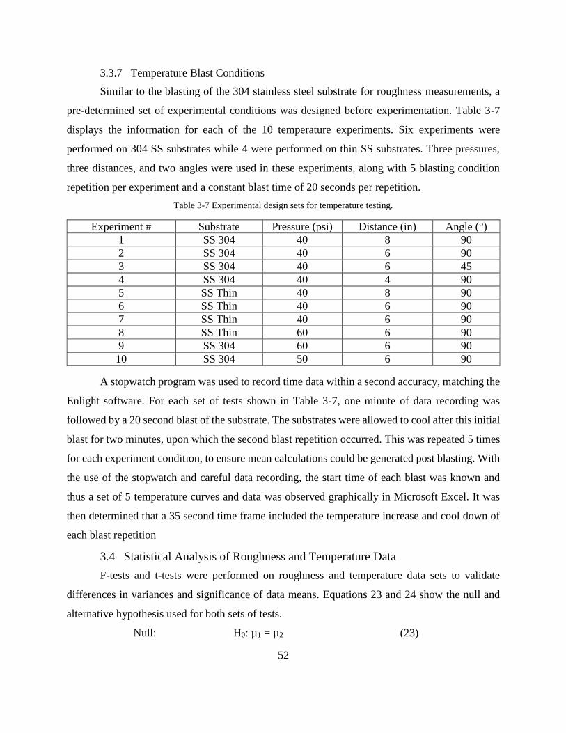
52

3.3.7 Temperature Blast Conditions

Similar to the blasting of the 304 stainless steel substrate for roughness measurements, a

pre-determined set of experimental conditions was designed before experimentation. Table 3-7

displays the information for each of the 10 temperature experiments. Six experiments were

performed on 304 SS substrates while 4 were performed on thin SS substrates. Three pressures,

three distances, and two angles were used in these experiments, along with 5 blasting condition

repetition per experiment and a constant blast time of 20 seconds per repetition.

Table 3-7 Experimental design sets for temperature testing.

Experiment # Substrate Pressure (psi) Distance (in) Angle (°)

1 SS 304 40 8 90

2 SS 304 40 6 90

3 SS 304 40 6 45

4 SS 304 40 4 90

5 SS Thin 40 8 90

6 SS Thin 40 6 90

7 SS Thin 40 6 90

8 SS Thin 60 6 90

9 SS 304 60 6 90

10 SS 304 50 6 90

A stopwatch program was used to record time data within a second accuracy, matching the

Enlight software. For each set of tests shown in Table 3-7, one minute of data recording was

followed by a 20 second blast of the substrate. The substrates were allowed to cool after this initial

blast for two minutes, upon which the second blast repetition occurred. This was repeated 5 times

for each experiment condition, to ensure mean calculations could be generated post blasting. With

the use of the stopwatch and careful data recording, the start time of each blast was known and

thus a set of 5 temperature curves and data was observed graphically in Microsoft Excel. It was

then determined that a 35 second time frame included the temperature increase and cool down of

each blast repetition

3.4 Statistical Analysis of Roughness and Temperature Data

F-tests and t-tests were performed on roughness and temperature data sets to validate

differences in variances and significance of data means. Equations 23 and 24 show the null and

alternative hypothesis used for both sets of tests.

Null: H0: µ1 = µ2 (23)

53

Alternative: H0: µ1 ≠ µ2 (24)

For roughness data, 10 Ra values were generated for each experiment set Fcalc values were created

based on Equation 25, where VarA and VarB are the variances for set A and set B.

𝐹𝑐𝑎𝑙𝑐 =𝑉𝑎𝑟𝐴

𝑉𝑎𝑟𝐵 (25)

Next Fcrit is selected from an F table, based on degrees of freedom for the roughness testing

which was 18 and 8 degrees of freedom for temperature F-tests. Two conclusions are made from

the F-test values, one assumption is that Fcalc < Fcrit, thus the variance of means is equal. The other

assumption is that from Fcalc > Fcrit meaning that variances are not equal. These assumptions are

shown as Equations 23 and 24 above. All comparisons made were at CI of 95% or α = 0.05. Under

optimum process scenarios, low spread of data or low variance from the mean is expected. When

variances are equal, 18 degrees of freedom for Ra comparisons and 8 degrees of freedom for

temperature comparison are used in the t-test calculations. When variances are not equal from the

F-test calculations, then different degrees of freedom are used in the t-tests, thus a different tcrit is

compared to each tcalc value from two-tailed t-tests.

Two-tailed t-tests were performed to determine if the means of each data set comparison

were significant. When tcalc < tcrit, with a pcalc > 0.05, then the means of each data set are not

different, thus no difference in blasting conditions is seen for that specific comparison.

Alternatively, when pcalc < 0.05 (high confidence) and tcalc > tcrit, then there is significance in two

means from two difference blasting conditions for roughness and temperature testing. Equation 26

shows the tcalc value based on equal variances in data. �̅� is the mean value for a data set, n is the

number of experiments in each set of data, and S is the standard deviation of each data set.

𝑡𝑐𝑎𝑙𝑐 =𝑥𝐴̅̅ ̅̅ −𝑥𝐵̅̅ ̅̅

√[(𝑛𝐴−1)∙𝑆𝐴

2 +(𝑛𝐵−1)∙𝑆𝐵2

(𝑛𝐴+𝑛𝐵−2)]∙[

[𝑛𝐴+𝑛𝐵]

[𝑛𝐴∙𝑛𝐵]]

(26)

A sample F-test and t-test calculation are shown in Appendix E. The calculated F value

(Fcalc) was less than the table F value (Fcrit), so variances were equal. When a two-tailed t-test was

performed with this set of data, the assumption of equal variances was used, which gives a tcrit at

18 degrees of freedom. The tcalc > tcrit, so there was a significance in means is present, thus the

blasting conditions affected the surface roughness parameter Ra for example.

54

4 Results and Discussion

4.1 Roughness Characterization Results

Surface roughness measurements occurred by using the SJ-210 Mechanical Profilometer,

HIROX optical microscope, and UVA ROST. Table 4-1 contains data obtained from

characterizing all 18 sets of blasting conditions with the SJ-210 mechanical profilometer. Ra, along

with values for other roughness parameters were gathered through mechanical profilometry and

average Ra, along with standard deviations for: measurements, average Ra, and process plus

measurements.

Table 4-1 SJ-210 Ra results with three types of standard deviation.

Sample Avg. Ra (µm) σM σAvg.Ra σP+M

1 3.89 0.26 0.23 0.34

2 3.67 0.18 0.15 0.22

3 3.45 0.19 0.14 0.23

4 3.36 0.27 0.10 0.25

5 4.47 0.31 0.19 0.35

6 4.24 0.23 0.11 0.26

7 4.08 0.27 0.18 0.31

8 3.98 0.29 0.31 0.41

9 5.01 0.34 0.24 0.40

10 4.67 0.33 0.20 0.38

11 4.50 0.35 0.27 0.43

12 4.68 0.39 0.22 0.44

13 4.70 0.34 0.24 0.41

14 4.18 0.28 0.42 0.49

15 4.23 0.46 0.40 0.63

16 4.47 0.36 0.23 0.42

17 4.35 0.36 0.24 0.42

18 4.23 0.30 0.24 0.37

Average Ra varied from a minimum of 3.45 µm for Experiment #3 to a maximum of 5.01

µm for Experiment #9. Experiment #2 had the smallest σM and σP+M between samples blasted

under the same condition, while Experiment #15 had the largest σM and #4 had the largest σP+M.

Experiment #6 had the lowest σAvg.Ra value, while Experiment #4 had the largest of these values.

The reason #4 had large values of standard deviation was due to sample 4.05 being rougher from

running out of media during blasting on the second pass.

55

Table 4-2 contains results of the HIROX data for substrate 2.10 and 3.10. The influence of

magnification and focal distances are shown for average Sa and σM. Using a smaller focal distance,

along with lower magnification led to smaller σ values. However, at higher magnification, a large

focal distance led to larger σ values. Based on these HIROX characterization methods, the Sa

results were more accurate for lower focal distances and lower magnification.

Table 4-2 Hirox measurements for Sa & σ calculations of samples 2.10 and 3.10.

Measurement Sample Magnification Focal Distance Avg. Sa σM

A. 2.10 350X 2m 3.858 0.240

B. 2.10 350X 4m 3.854 0.248

C. 2.10 700X 4m 4.189 0.395

D. 2.10 700X 2m 4.180 0.403

E. 3.10 350X 2m 3.377 0.221

F. 3.10 350X 4m 3.368 0.227

G. 3.10 700X 4m 4.133 0.340

H. 3.10 700X 2m 4.144 0.338

The last characterization utilized for roughness characterization was the optical

profilometry method via the UVA ROST. Only samples from four different blasting conditions

were measured and the results of average Sa and σM are shown below in Table 4-3. According to

this set of data, sample 2.10 had the largest Sa value 4.46 µm and sample 4.06 had the lowest Sa

value of 3.44 µm. Sample 3.09 had the smallest σM, while sample 4.08 had the largest σM.

Table 4-3 ROST Avg. Sa and measurement σ values.

Sample # Avg. Sa σM

1.03 4.358 0.508

2.05 4.062 0.488

2.06 3.860 0.524

2.07 4.422 0.254

2.08 4.300 0.264

2.09 4.236 0.412

2.10 4.458 0.422

3.08 3.827 0.338

3.07 3.894 0.540

3.09 3.827 0.248

3.10 3.863 0.450

4.06 3.442 0.662

4.07 3.602 0.460

4.08 3.534 0.729

4.09 3.824 0.411

56

4.10 4.173 0.702

Table 4-4 contains results from the three characterization techniques used to obtain average

roughness parameters Ra and Sa. It can be noted that for each sample set (blasting condition), the

SJ-210 took ten measurements per substrate, for ten substrates. The UVA ROST used ten

measurements per blasting condition, however only a few of the samples from each of the four

blasting conditions were tested, thus standard deviation values were high. The HIROX microscope

was utilized to calculate Ra for only two substrates. The Hirox measurement σ values were lower

due to the measurement accuracy from fifteen measurements taken per substrate. Based on the low

σ values, relative quickness of data collection, and device availability, the SJ-210 mechanical

profilometer was utilized as the main roughness characterization device in the following sections.

Table 4-4 Comparison of Ra and σM for characterization techniques.

Sample Set Mitutoyo SJ210 Profilometer UVA ROST UVA Hirox

Ra (µm) σM Ra (µm) σM Ra (µm) σM

1 3.89 0.26 4.358 0.508 - -

2 3.67 0.18 4.223 0.394 3.854 0.240

3 3.45 0.19 3.853 0.394 3.377 0.221

4 3.36 0.27 3.798 0.593 - -

4.2 Effect of Process Parameters on Surface Roughness

As shown in Table 3-4, the surface roughness experiments differed based upon blast height,

blast pressure, nozzle type, blasting operator, and blasting on different days under the same

conditions. With the use of JMP statistical analysis software, data was gathered from the various

18 blasting conditions to generate Figure 4.1. Figure 4.1 showed that a shorter blast distance 4”

led to rougher surface than the higher blast distance of 6”. These results were statistically compared

with 95% confidence under an F-test, which showed that the variance of each set of data were

equal. Once the F value was calculated, a two-tailed t-test was performed with an alternative

hypothesis that distance changes would affect roughness values. A tcalc value of 2.52, with

probability (pcalc = 0.022 < pcrit = 0.05) was larger than tcrit of 2.10 with the calculation of degrees

of freedom = 18. With the t-test results under 95% confidence, it is proven that a shorter blast

distance (4”) lead to a rougher surface than larger distance (6”) by 0.22 µm, as Ra changed from

3.89 µm +- 0.07 µm to 3.67 µm +-0.05 µm. Appendix F contains results from Microsoft Excel

57

for these F-tests and t-tests under these blasting conditions, as well as all other statistical results

for roughness data.

Figure 4.1 Blast distances effects on Ra for 4” and 6” blasting.

A similar comparison was made between blast distances of 6” and 8” to show the same

effect on surface roughness and is shown in Figure 4.2. The F value was calculated to be 1.15,

which was smaller than Fcrit of 3.18 with pcrit being 0.42 > 0.05, thus the variances of the means

were equal. Next a two-tailed t-test was performed with the same alternative hypothesis that a

distance change would affect surface roughness values. The tcalc value was calculated as 3.49, while

tcrit is 2.10 and pcalc is 0.0026. With 95% confidence, blasting at 6” led to a higher Ra than 8”

blasting by a difference of 0.22 µm from 3.67 µm +-0.05 µm to 3.45 µm +-0.04 µm.

Figure 4.2 Blast distance effects on Ra for 6” and 8” blasting.

When blasting stainless steel substrates with alumina grit, an increase in surface roughness

with increasing blasting pressure is expected, according to studies of other research groups [23].

58

Figure 4.3 suggests the opposite trend, so this comparison between 42 psi and 60 blasting was then

compared with F-test and t-test to see if lower pressure actually lead to rougher surfaces than

higher pressure. Fcalc = 1.39 and pcalc = 0.32 led to the use of a two-tailed t-test with the assumption

of equal variances between means. The two-tailed t-test gave tcalc = 3.42, with pcalc = 0.0031, thus

with 95% confidence, it was proved that blasting at 42 psi led a rougher surface by 0.33 µm

difference from 60 psi blasting or change from 5.01 µm +-0.08 µm to 4.68 µm +-0.06 µm.

Figure 4.3 Blast pressure effect on Ra for 42 psi and 60 psi blasting.

The nozzle type, whether 3/16” Venturi or 5/16” straight was expected to affect the surface

roughness differently. Based on nozzles of the same throat dimensions, it is assumed that Venturi

nozzles would create higher roughness values than straight nozzles. Figure 4.4 displays the effects

of 5/16” straight nozzle and the 3/16” Venturi nozzle of surface roughness, with the use of as

received media. First an F-test was performed to once again see if the variances between means

for the 5/16” straight and 3/16” Venturi nozzles were actually different. Fcalc = 4.7 > Fcrit = 3.18,

with pcalc = 0.015, thus the null hypothesis of the variances being equal was false. Next a two-tail

t test was performed with the assumption of unequal variances. The tcalc =0.072, with pcalc = 0.94,

so with 95% confidence the null hypothesis of the 5/16” straight nozzle creating a higher roughness

than 3/16” Venturi by 0.01 µm was rejected. The reason for the higher surface roughness is due to

the larger diameter throat of the 5/16” straight nozzle when compared to the 3/16” Venturi nozzle.

59

Figure 4.4 Nozzle type effect on Ra.

As mentioned previously, pulsating media or irregular media flow would lead to a

difference in surface roughness modifications. As Figure 4.5 denotes, experiments performed with

pulsating media flow created a lower surface roughness when compared to blasting where

pulsation did not occur. The Fcalc = 2.64 with pcalc =0.082, thus it was determined the variances of

means for non-pulsating and pulsating media flows were not equal. For the two-tailed t-test, tcalc =

6.38 with pcalc = 5.3 x 10-6, thus with 95% confidence it was concluded that pulsation will decrease

the roughening effect of blasting by 0.56 µm, going from 4.23 µm +-0.08 µm to 3.67 µm +-0.05

µm.

Figure 4.5 Media flow effect on Ra.

The effect of media break done or recycled media (age) is shown in Figure 4.6. An F-test

of the data proved that variances were equal since Fcalc = 1.01, with pcalc = 0.49. The alternative

hypothesis was that broken down media would lead to a smoother surface than newer media.

60

However, due to tcalc = 4.31 and pcalc = 4.18 x 10-4, with 95% confidence the old media (smaller

media) led to rougher surfaces than newer (larger) media by 0.47 µm as Ra increased from 4.23

µm +-0.08 µm to 4.70 +- 0.08 µm. The new media generated lower surface roughness values since

the media velocity was lower and the blast pattern was less dense, but had larger particles eroding

the substrate surface.

Figure 4.6 Media Recycling effect on Ra.

4.3 Repeatability and Reproducibility

Three areas that were investigated along with process parameter variation, were the use of

two different cabinets, two blast operators, and one blast operator blasting under same conditions

at different times. Figure 4.7 shows the Ra differences when blasting under the same conditions,

with blasting occurring almost one week apart between “Day A” and “Day B”.

Figure 4.7 Repeatability of same blast conditions.

An F-test was performed, which gave Fcalc = 1.03 at pcalc = 0.049, so the variance between

means of “Day A” and “Day B” were equal. A two-tailed test was performed next since there was

61

no expected or hypothesized difference for blasting under the same conditions on different days.

The tcalc = 2.94 at pcalc = 0.0087, thus it was shown with 95% confidence since the two-tailed tcrit =

2.10 (df = 18) that blasting under the same conditions on different days does effect surface

roughness. There was a difference in Ra mean values (significance) due to shorter blast times on

average from Day A to Day B and low Ra for one substrate on Day B, however there was no

variance between the data sets.

Another area investigated was the difference in surface roughness from using two different

blast cabinets: CCAM 3642 and VT 4848. Figure 4.8 shows the differences in Ra for the two

different cabinets. The F-test gave Fcalc = 1.07 with pcalc = 0.46, thus the variances of cabinet mean

Ra values were equal. Another two-tailed t-test was performed with the null hypothesis that the

different cabinets would not affect Ra. At 95% confidence, the tcalc = 4.34 and pcalc = 3.98 x 10-4,

the null hypothesis was rejected. An increase in Ra of 0.46 µm was shown when switching from

the CCAM cabinet to the VT cabinet as roughness increased from 3.89 µm +-0.07 µm to 4.35 µm

+- 0.08 µm.

Figure 4.8 Cabinet type effect on Ra.

The last area of process variation occur when using two different operators to blast under

the same conditions. Figure 4.9 contains Ra values gathered from two blast cabinet operators from

the VT cabinet. The F-test gave Fcalc = 1.15 with pcalc = 0.42, thus the variances between operator

mean Ra were equal. The two tailed t-test was performed next, with the null hypothesis that the

mean Ra values for different operators would be the same. At 95% confidence, tcalc = 1.98 with

pcalc = 0.064, there was no statistical difference in the means of “Operator A” (novice) and

“Operator B” (experienced).

62

Figure 4.9 Operator effect on Ra.

Visual inspection showed distinct differences in surface texture between experienced and

novice operators. This detectable difference is shown below in Figure 4.10 with a comparison of

good (experienced operator) blasting coverage and bad (novice operator) blasting coverage. The

novice blaster created blast lines on the surface, whereas the experienced operator generated more

even coverage of the substrate.

Figure 4.10 a. Good coverage & b. bad coverage.

4.4 Temperature Sensor Measurements

Some small-scale experiments were performed prior to the blasting of the stainless steel

substrates with the attached temperature probe. One of these experiments showed the effect of

adding additional adaptors to the fiber strand connected between the “TempSens1” on an

aluminum substrate and the SM125 Interrogator. For this experiment, no blasting occurred, the

cabinet doors were shut and the dust collection system was on. Figure 4.11 shows that when adding

additional adaptors, an increase in temperature reading occurred with the addition of each adaptor,

suggesting that signal lose would for this system show an increase in substrate temperature without

a. b.

63

blasting occurring. There was clear distinction in the temperature readings as well, with no

overlapping temperatures.

Figure 4.11 Adaptor effect on substrate temperature.

Another set of experiments performed prior to any blasting of the SS substrates monitoring

the temperature of an aluminum substrate with different light sources. Another clear distinction

was noticed when having the light source, either Halogen or LED turned on for three hours with

no blasting occurring using the temperature sensor on the Al substrate to monitor substrate

temperature as shown in Figure 4.12. The Halogen light showed an increase in temperature from

17°C to 30°C, over the three hour span. The halogen light was replaced with the LED light and the

temperature change of the same substrate only saw an increase around 0.5 °C. For the purposes of

understanding temperature in the blast cabinet and the substrate temperature, the LED light source

was used to help eliminate any external temperature effects.

Figure 4.12 LED and halogen effect on substrate temperature.

The last set of experiments performed with temperature sensor were on five different

stainless steel substrates to show the effect of temperature change from changing the blast distance

64

of each experiment. The experimented were performed in this order for the following distances:

8”, 2”, 6”, 4” and 10” and mean data is shown in Figure 4.13.

Figure 4.13 Blast height effect on substrate temperature with “TempSens2”.

The first three tests showed was to be expected, decreasing the blast height would lead to

higher temperature. The last two experiments with blast height of 4” and 10” did not follow this

trend. The temperature changes are scattered, but the use of additional duct tape and media age

were the reasons for the differences in the expected and unexpected results shown in Figure 4.7.

With these results, it was decided that the temperature probe might give more valid temperature

readings, as well as a higher accuracy when using the probe.

4.5 Temperature Probe Measurements

For this set of experiments, a total of 10 different blast conditions were utilized to show

differences in effects of blasting pressure, angle, distance, and substrate shape. Each set of

experiment was performed at least 5 times, so average data could be gathered from each individual

experiment. Figure 4.14 shows an example of raw blasting data after the start of each blast time

was zeroed out using the timestamps from the Enlight Software and the stopwatch data for

Experiment #1.

65

Figure 4.14 Experiment #1 data.

In order to compare data from these experiments, the data had to be zeroed out by

subtracting the initial temperature value from each repetition curve of each experiment. Figure

4.15 contains a graphical representation of “zeroed” data from experiment #1. Once the data was

zeroed, average curves of each experiment could be obtained for comparison of effects of blast

angle, pressure, distance, and substrate type.

Figure 4.15 Zeroed temperature experiment #1 data.

Table 4-5 shows results of the “TempProb2” measurements on the 304 stainless steel

substrates. One row contains the average of five temperature changes that occurred from blasting

condition after 20 seconds of blasting had occurred, while the last two rows display the standard

deviation and error of those values. Based on this table, the lowest temperature change occurred

from blasting condition #3 (40 psi, 6” distance, and 45° angle) and the highest temperature change

occurred at blasting condition #9 (60 psi and 6” distance). Experiments from Table 4-5 show that

as blast distance decreases, substrate temperature from blasting saw a larger temperature increase.

Higher blast pressures lead to higher temperature increases in 304 stainless steel substrates and

angled blasting reduced the temperature increase of the substrates.

66

Table 4-5 304 Stainless steel substrate temperature results.

Experiment # 1 2 3 4 9 10

Pressure (psi) 40 40 40 40 60 50

Distance (inch) 8 6 6 4 6 6

Angle (°) 90 90 45 90 90 90

T (°C) at 20 sec 21.7 19.9 8.3 29.1 45.1 35.2

σ 3.0 3.5 0.9 4.1 4.9 2.6

Error 1.3 1.6 0.4 1.8 2.2 1.1

In order to justify these results, F-tests and t-tests were performed for validation. Appendix

G contains the calculations for these tests for the blasting condition comparison of 4” and 6”

distance blasting 304 SS for temperature effect differences. For this comparison, Fcrit was found

from the F table to be 6.39 and Fcalc was 1.34 at pcalc = 0.39, so the variance of the means were

equal. Performing a two-tailed t-test gave tcalc = 3.79 at pcalc = 0.005 when tcrit = 2.31, so at 95%

CI a substrate ΔT occurred when blast distance changed from 6” to 4”. For this case, ΔT= +9.2 °C

from the 6” T of 19.9 °C +-1.6 °C to the 4” T of 29.1 °C +- 1.8 °C. Another distance test occurred

when changing the blasting distance from 6” to 8”, with an Fcalc = 1.40 at pcalc = 0.38, so a two-

tailed t-test was performed with an equal mean variances assumption. The tcalc was 0.89 and pcalc

= 0.41, so with 95% confidence no distinction can be made between the 6” blasting and 8” blasting

effects on 304 SS ΔT. F test and t test values are in Appendix G as well, Figure 4.16 shows a

graphical representation of the temperature changes in 304 SS from different blast distances.

Figure 4.16 Blast distance effects on 304 SS temperature changes.

67

When comparing the pressure changes from 40 psi to 50 psi, Fcalc = 1.90 and pcalc = 0.27,

so variances were equal and thus a two-tailed t-test was performed assuming equal variances. The

tcalc was 7.79 at pcalc = 5.3 x 10-5, so with 95% confidence +ΔT of 15.3 °C occurred when going

from the lower pressure (40psi) T = 19.9 °C +- 1.6 °C to medium pressure (50 psi) T =35.2°C +-

1.1 °C. Next a comparison of 50 psi and 60 psi blasting occurred, giving Fcalc = 3.60 at pcalc = 0.12,

so another assumption of equal variances was made when performing a two-tailed t-test. The tcalc

= 4.03 with pcalc = 0.0038, so at 95% confidence, increasing the blasting pressure of 50 psi to 60

psi led to an 304 SS +ΔT of 9.9 °C from T = 35.2°C +- 1.1 °C to T = 45.1 °C +- 2.2 °C. Figure

4.17 displayed these effects of blasting pressures on 304 SS temperature. Higher pressures lead to

higher particle impact speeds, thus more heat is generated with increasing pressure.

Figure 4.17 Pressure effect on 304 SS temperature.

The last set of temperature testing for 304 stainless steel substrates was changing the blast

angle from 90° to 45°. An F-test was performed for variances, giving Fcalc of 14.01 and pcalc =

0.013, so unequal variances were present between data means. The tcalc value of 7.09 and pcalc 8.7

x 10-4 under 95% confidence validated the significance in means through a two-tailed t-test with

tcrit being 2.57 (degrees of freedom = 5). A –ΔT = 11.6 °C was seen from the 19.92 °C +-1.6°C for

90° blasting to 8.3 °C +- 0.4 °C for 45° blasting. These results are shown graphically in Figure

4.18 for 20 seconds of blasting, showing that a lower angle leads to a lower increase in temperature.

As the blast angle gets shallower, the blast pattern will get larger, leading to a lower temperature

change in substrate temperature.

68

Figure 4.18 Angle effect on 304 SS temperature.

The thin stainless steel substrates were subjected to tests of blast distance, pressure, and

angle effects as well. Table 4-6 shows temperature data for thin stainless steel substrates. Based

on this data, the blast distance showed the same trend as the 304 SS of decreasing distance leading

to a larger temperature change in thin SS substrate temperature. The values of experiments #6, #7,

and #8 were very close in value, thus more F-tests and t-tests were performed.

Table 4-6 Thin stainless steel substrate temperature results.

Experiment # 5 6 7 8

Pressure (psi) 40 40 40 60

Distance (inch) 8 6 6 6

Angle (°) 90 90 45 90

T (°C) at 20 sec 14.3 24.1 23.5 24.9

σ 1.7 4.5 2.4 5.1

Error 0.8 2.0 1.1 2.3

Distances of 6” and 8” variance in means were compared with F-tests giving Fcalc = 7.28

and pcalc of 0.040, thus variances were not equal. Performing a two-tailed t-test gave tcalc = 4.56

and pcalc = 0.0061, thus with 95% confidence the difference in means was significant. For this case,

decreasing the blast distance from 8” to 6” led to +ΔT of 9.8 °C from 14.3 °C +-0.8 °C to 24.1 °C

+- 2.0 °C. This trend matched up with the trend noticed in the blasting of 304 SS at distances of

4” and 6”. Decreasing the blast distance leads to a more concentrated or smaller blast diameter

pattern, thus more impact energy is concentrated near the temperature probe, creating larger ΔT

values. Figure 4.19 shows the differences in blasting at 6” and 8” for the thin stainless steel

substrates.

69

Figure 4.19 Blast distance effect on thin SS temperature.

Next the pressure effects on thin stainless steel substrates from blasting were analyzed and

the results are shown in Figure 4.20. An F-test was performed between the T means for 40 psi and

60 psi data sets, giving Fcalc = 1.26 and pcalc = 0.41, so equal variances were present. The alternative

hypothesis through a two-tailed t-test was that different pressures would lead to different ΔT for

thin SS when blasting, however due to tcalc being 0.26 and pcalc = 0.80 no distinction could be made

at 95% confidence for this blast condition.

Figure 4.20 Blast pressure effect on thin SS temperature.

The last set of comparisons made for thin SS was changing the blast angle from 90° to 45°.

Performing an F-test gave Fcalc = 3.65 and pcalc = 0.12, so a two-tailed t test was performed

assuming equal variances. The tcalc was 0.27 and pcalc = 0.79, so no distinction could be made

between the angled and perpendicular blasting of the thin SS with 95% confidence. Figure 4.21

shows the graphical representation of the angle effect on temperature changes in thin SS substrates.

70

Figure 4.21 Blast angle effect on thin SS temperature.

The last set of comparisons to be validated through F-tests and t-tests were by comparing

data from the 304 SS and thin SS blasting at the same conditions to view the importance of

substrate thickness/shape. At 6” blast distance the Fcalc was 1.63 and pcalc was 0.32, so equal

variances were present between means of 304 SS and thin SS substrates. The tcalc was 1.64 and

pcalc = 0.14, so no distinction could be made between substrate effect on temperature change at 6”

blasting with 95% confidence. At 8” blast distance the Fcalc was 3.18 and pcalc = 0.15, so variances

were present again for the two-tailed t-test. The tcalc was 4.85 and pcalc was 0.0013, so with 95%

confidence a substrate effect was detectable at 8” blasting. For this case, +ΔT of 7.4 °C occurred

when going from a thin SS T = 14.3 °C +-0.8 °C to thick SS T = 21.7 °C +-1.3 °C.

Blasting at 60 psi pressure and blasting at the 45° angle were compared between 304 SS

and thin SS substrate temperature changes as well. For the 60 psi blasting condition, the Fcalc was

1.09 and pcalc was 0.47, so a two-tailed t-test was performed assuming equal variances of means

between 304 SS and thin SS data sets. The tcalc was 6.41 and pcalc = 2.1 x 10-4, so +ΔT was seen

with 95% confidence. For this scenario ΔT = 20.2 °C from the thin SS T = 24.9 °C +- 2.3 °C to

thick SS T = 45.1 °C +- 2.2 °C. The angled blasting Fcalc was 6.27 and pcalc was 0.052, so variances

were equal for the two-tailed t-test. The tcalc was 13.35 and pcalc was 9.5 x 10-7, so with 95%

confidence ΔT between substrate type/shape occurred at 45° blasting. That temperature -ΔT = 15.2

°C from the thin SS T = 8.3 °C +-1.1 °C to 304 SS T= 23.5 °C +- 0.4 °C.

71

5 Conclusions Blasting process parameters affect the surface roughness generated and the amount of

temperature change in the substrate. Based on the surface roughness experiments, conclusions

could be made based on: blast distance, pressure, angle, time, recycled media, media pulsation,

nozzle type, operator experience, blast date, and blast cabinets. The results of the experiments

proved that decreasing the blast distance led to higher surface roughness values due to the smaller

blast pattern generated when being closer to the substrate with the blast nozzle. With 95%

confidence, ΔRa = 0.22 µm when going from 6” to 4” distances and a ΔRa = + 0.22 µm when

going from 8” to 6” distances. SJ-210 measurements proved that ΔRa = -0.33 µm from 42 psi to

60 psi blast pressures. Blast angle was shown to have numerous effects on the substrate roughness.

Generally, a decrease in the blast angle lead to a more erosive effect on the stainless steel substrate

surface. Blast time can lead to an over blasting effect after a certain optimum blast time (maximum

roughness was obtained). Based on these individual parameters, a combination of a shorter

distance and lower blast pressure would generate the highest Ra values.

The type of nozzle will create differences in surface roughness when the inner throat

diameter of the straight nozzle and Venturi nozzles are the same. When the throat sizes are the

same, the Venturi nozzle would lead to a wider spread blast pattern and an increase in roughness

would occur due to higher media velocities. However, a 3/16” Venturi and 5/16” straight nozzle

were used in experiments, thus the throat sizes were not the same. At 95% confidence, the straight

nozzle and Venturi nozzle created no significant difference in means. Media pulsation created an

issue with surface roughness and it was shown through experiments that pulsating media led to a

lower surface roughness change than non-pulsating or regular media flow rates by ΔRa = -0.56

µm. Recycled media through experimentation over different blast cycles under the same blasting

conditions proved to lead to lower Ra values due to smaller particles creating a denser blast pattern

by 0.47 µm.

The same operator blasting under same conditions was investigated, showing that ΔRa

decreased in later experiments due to shorter average blast times and one substrate with low Ra,

and equal variances were present. Using different cabinets under the same blast conditions

generated ΔRa, with the CCAM PF-3642 creating slightly smoother surfaces than the substrates

72

blasted with the VT PF-4848 ΔRa = 0.46 µm. Blasting with two difference operators did not

significantly affect ΔRa.

Various tests occurred through changing the process parameters of blasting 304 SS and

thin SS substrates for investigation of substrate ΔT from blasting. With 95% confidence, changing

the blast distance from 6” to 4” led to a substrate ΔT = +9.2 °C for 304 SS substrates due to the

blast pattern being more concentrated near the temperature probe. No statistical distinction could

be made when blasting between 6” and 8”. When blasting at different pressures, positive ΔT

occurred with increasing pressure. When going from 40 psi to 50 psi, the ΔT = +15.3 °C and ΔT

= +9.9 °C when pressure changed from 50 psi to 60 psi on 304 SS substrates due to higher impact

velocities of grit particles. The blast angle affected the substrate temperature proportionally, when

the lower blast angle to 45° was utilized ΔT = -11.6 °C from 90° blast angle. This affect can be

attributed to the larger blast pattern generated at lower angles. Having a perpendicular blast angle,

with higher pressure and low blast distances would lead to the largest 304 SS substrate ΔT.

For thin SS, process parameters were changed similar to the 304 SS temperature testing.

As the blast height decreased from 8” to 6”, the blast pattern radius increased, leading to ΔT= +9.8

°C. The angled blasting and pressure blasting of the thin SS substrates generated higher

temperatures than the 8” distance testing. However no distinction could be made with 95%

confidence when changing the angle or pressure.

The other expected results were that the shape or thickness of the substrate would lead to

different temperature changes when blasting. When blasting the thin SS and 304 SS substrates, no

distinction could be made between the substrate temperatures at 6” distance. However, viewing

the effect of substrate thickness or shape at 8” blast distance showed that a ΔT = +7.4 °C when

switching from the thin SS to 304 SS. Similar effects were seen when blasting different substrates

at the same 45° and another experiment at 60 psi. A ΔT = +20.2 °C occurred for the angled blasting

and ΔT = -15.2 °C for the higher pressure blasting when switching from the thin SS to 304 SS

substrates. Based on these results, with 95% confidence the substrate thickness or shape does play

a role in the temperature generated from blasting under conditions of a larger standoff distance,

45° angle, and higher pressure.

73

6 Future Work Based on the results of these experiments, further investigation is needed in the following

areas for purposes of understanding surface roughness changes from process parameter variation.

For any future testing, use new media for each set of experiments for different blast conditions,

this would allow for more refined results. Another set of experiments would be to use different

media types or sizes and follow up on other literature and add in experiments to better understand

lacking areas for a given media/substrate combinations. Since blast time and blast angle were not

varied for the roughness tests, other experiments could use three different blast angles and three

different blast times to show more distinct changes in roughness values. A better understanding of

the repeatable and reproducible experiments with different blast cabinets, blast operators, and same

operator re-running experiments would be interesting to see how roughness would be altered if

new media was used in all experiments. Future work for roughness data would also contain

interactions of the various altered parameters, to optimize generating the highest Ra values

possible.

For purposes of measuring ΔT from blasting, more temperature probes or sensors would

help better illustrate the effects from different process parameters. If the media flow rate would

controlled with an automatic media flow regulator, media flow effects on temperature could be

better understood. Using different size/type of media and different substrate materials, shapes, and

sizes would be of interest to learn more about the thermal changes generated from blasting.

Calculations of ΔT on the side of the substrate being blasted would be of interest as well. Strain

gage testing on the substrates during blasting would be beneficial to understand the effects of the

thermal strain and change in refractive index of the fibers.

Other areas of interest would be to combine the roughness and temperature testing into one

set of experiments. Results would show the effects of roughness on the surface and various

conclusions would be gathered from knowing how much the temperature change affects the quality

of the substrate surface. These tests could be combined with strain testing, along with other types

of characterization techniques for in-situ blasting and post blasting.

74

References [1] Tilghman, B.C. “Improvement in Cutting and Engraving Stone, Metal, Glass, etc. US States Patent 108,408.”

Copyright October 18, 1870.

[2] No Author. “The Difference Between Surface Profile and Class of Blast.” Blast One. Copyright 2014. Online:

http://www.blast-one.com/weekly-tips/the-difference-between-surface-profile-and-class-of-blast

[3] Rettermayer, Robert. “The History of Sandblasting”. Gero Sandblasting. Copyright 2013. Online:

http://www.sand-blasting.co/the-history-of-sandblasting/

[4] No Author. “Progressive Surface History.” Progress Surface. Copyright 2014. Grand Rapids, Michigan. Date

Accessed: January 22, 2014. Online: http://www.progressivesurface.com/company.php

[5] Momber A. Blast Cleaning Technology: Chapter 1: Introduction. Springer. Copyright 2008. Berlin,

Heidelberg. Pages 1-6. Online: http://link.springer.com/chapter/10.1007/978-3-540-73645-5_1

[6] No Author. “Blast Cabinets.” Norton Sandblasting Equipment. Chesapeake, VA. Copyright 2014. Online:

http://www.nortonsandblasting.com/nsbcontact.html

[7] No Author. “Abrasive Blast Equipment: Pressure versus Suction.” Surface Preparation. Copyright 2014.

Online: http://www.surfacepreparation.com/abrasive-blast-equipment-pressure-versus-suction

[8] Heywood, H. “Numerical Definition of Particle Size and Shape.” Chemical Ind. Copyright 1933. Volume

32. Pages 149-154.

[9] Vasek, J., Martinec, P., Foldyna, J. “Influence of properties of garnet on AWJ Cutting Process”. Proc. 7

Am. Water Jet Conference. Water Jet Technology Association. St. Louis, Missouri. Copyright 1993.

Volume 1. Pages365-387.

[10] Wadell, H. “Sphericity and Roundness of Rock Particles.” J. Geol. Copyright 1933. Volume. 41. Pages

316-331.

[11] Hansink, J.D. “Economics of Abrasive Selection for Shipyard Use.” Protective Coatings Europe. Copyright

1998. Volume 3. Issue 5. Pages 24-27.

[12] Bohemia Garnet & Momber A. Blast Cleaning Technology: Chapter 2: Abrasive Materials. Springer.

Copyright 2008. Berlin, Heidelberg. Page 21.

[13] Bahadur, S., Badruddin , R. “Erodent Particle Characterization and the Effect of Particle Size and Shape on

Erosion.” Wear. 1990. Volume 138. Pages 189-208.

[14] Momber A. Blast Cleaning Technology: Chapter 2: Abrasive Materials. Springer. Copyright 2008. Berlin,

Heidelberg. Pages 7-53. Online: http://link.springer.com/chapter/10.1 007% 2F978-3-540-73645-5_2

[15] Kuhmichel GmbH & Momber A. Blast Cleaning Technology: Chapter 2: Abrasive Materials. Springer.

Copyright 2008. Berlin, Heidelberg. Page 18.

[16] No Author. “What is Grit Blasting?” Progressive Surface. Grand Rapids, Michigan. Online:

http://www.progressivesurface.com/gritblasting_process.php

[17] No Author. “What is Shot Peening?” Progressive Surface. Grand Rapids, Michigan. Online:

http://www.progressivesurface.com/shotpeening_process.php

[18] Metabrasive Ltd. & Momber A. Blast Cleaning Technology: Chapter 2: Abrasive Materials. Springer.

Copyright 2008. Berlin, Heidelberg. Page 18.

[19] No Author. “Particle Size Conversion Table. Sigma-Aldrich Co. LLC. Copyright 2013. Online:

http://www.sigmaaldrich.com/chemistry/stockroom-reagents/learning-center/technical-library/particle-size-

conversion.html

[20] Kelly, E.G., Spottiswood, D.J. Introduction to Mineral Processing. John Wiley & Son. Copyright 1982. New

York. Pages 21-45. Date Accessed: March 31, 2013.

[21] No Author. “Abrasives & Compounds.” Newport Glass Works, LTD. Stanton, CA. Copyright 2013. Online:

http://www.newportglass.com/grit.htm

[22] No Author. “Grit Size Conversion Table.” Media Blast & Abrasive, Inc. Copyright 2013. Online:

http://www.mediablast.com/grit-size-conversions.php

[23] Day, J., Huang, X., Richards, N.L. “Examination of a Grit-Blasting Process for Thermal Spraying Using

Statistical Methods.” Journal of Thermal Spray Technology. 2005. Volume 14. Pages 471-479.

[24] Maruyama, T., Akagi, K., Kobayashi, T. "Effects of Blasting Parameters on Removability of Residual Grit."

Journal of Thermal Spray Technology. 2006. Volume 15. Issue 4. Pages 817-821.

75

[25] Boerio, F.J., Roby, B., Dillingham, R.G., Bossi, R.H., Crane, R.L. "Effect of Grit-Blasting on the Surface

Energy of Graphite/Epoxy Composites." The Journal of Adhesion. 2006. Issue 82. Pages: 19-37.

[26] No Author. “Hardness.” The Free Dictionary. Farlex, Inc. Copyright 2013. Online:

http://encyclopedia2.thefreedictionary.com/Hardness+(materials+science)

[27] Tabor, D. The Hardness of Metals. Claredon Press. Copyright 1951.

[28] No Author. “Knoop Hardness.” Merriam Webster Dictionary. Merriam-Webster, Incorporated. Copyright

2013. Online: http://www.merriam-webster.com/dictionary/knoop%20hardness

[29] No Author. “Rockwell Testing.” Wilson Hardness. Copyright 2013. Online: http://www.wilson-

hardness.com/Resources/RockwellTesting/tabid/80/language/en/Default.aspx

[30] No Author. "Hardness Tables." Ted Pella, Inc. Copyright 2013. Online:

http://www.tedpella.com/company_html/hardness.htm

[31] No Author. “Hardness Conversion Chart.” NDT Resource Center. Online: http://www.ndt-

ed.org/GeneralResources/HardnessConv/HardnessConv.htm

[32] Wellinger, K., Uetz, H. Gleitverschleiß, Sp¨ulverschleiß, Strahlverschleiß unter der Wirkung

von k¨ornigen Stoffen. VDI-Forschungshefte, Copyright 1955. No. 449, 1–40.

[33] Uetz, H. Abrasion und Erosion. Carl Hanser Verlag, M¨unchen-Wien. Copyright 1986.

[34] Wellinger, K., Uetz, H., Gommel, G. G¨utekennwerte von Strahlmitteln und deren Ver¨anderung w¨ahrend

des Strahlvorganges. Stahl Eise, Copyright 1962. Vol. 82, No. 21, 1436–1445.

[35] No Author. "Abrasive-Blast Media Chart." Norton Sandblasting Equipment. Copyright Unknown. Online:

http://www.nortonsandblasting.com/nsbabrasives.html

[36] Makova, I., Sopko, M. "Effect of Blasting Material on Surface Morphology of Steel Sheets." Acta

Metallurgica Slovaca. Copyright 2010. Volume 16. Issue 2. Pages 109-115.

[37] No Author. “Fracture Stress.” Answers Corporation. Copyright 2013. Online:

http://www.answers.com/topic/fracture-stress

[38] Huang, H., Zhu, X.H., Huang, Q.K. “Weibull strength distributions and fracture characteristics of abrasive

materials.” Engineering Fracture Mechanics. Copyright 1995. Volume 23, Pages 773-776.

[39] Verspui, M.A., With, G., Dekkers, E.C. “A crusher for single particle testing.” Reviewed Scientific

Instruments. Copyright 1997. Volume 63. Issue 3. Pages 1553-1556.

[40] No Author. ISO 11124/2-4. Preparation of steel substrates before application of paints and related products

- Specifications for metallic blast-cleaning abrasives - Part 2: Chilled-iron grit. International Organization

for Standardization. Geneva. Copyright Unknown.

[41] SSPC-AB 2.Abrasive Specification No. 2: Cleanliness of Recycled Ferrous Metallic Abrasives. Revised

version. The Society of Protective Coatings. New York. Copyright 2004.

[42] Callister, Jr., W.D., Rethwisch, D.G. Fundamentals of Materials Science and Engineering: An Integrated

Approach. John Wiley & Sons, Inc. Copyright 2008.

[43] Tosha, K., Iida, K. "Residual Stress on the Grit Blasted Surface." Metal Behaviour & Surface Engineering.

Copyright 1989. Pages 323-328.

[44] Crithclow, G. Handbook of Adhesion Technology: Chapters 7 & 8. Loughborough, UK. Loughborough

University. 2011: Pages 119-177. Online: http://link.springer.com/referencework entry/10.1007/978-3-642-

01169-6_7

[45] Bacova, V., Draganovska, D. "Analyses of the Quality of Blasting Surfaces." Materials Science. 2004.

Volume 40. Issue 1. Pages 125-131.

[46] Acton, S., Agnew, S., Fitz-Gerald, J. CCAM Surface Characterization Interim Report. Charlottesville, VA.

University of Virginia. Pages 1-24.

[47] Tosha, K., Iida, K. "Crystal Transformation of Austenitic Stainless Steel by Shot Peening and Grit Blasting."

International Conference on Shot Peening and Blast Cleaning. Pages 111-120.

[48] Smith, T., Crane, R. Proceedings of the National SAMPE Symposium. Copyright 1980. Page: 25.

[49] Minford, J. “Aluminum 57.” Copyright 1981. Issue 10. Page: 657.

76

[50] Fang, C.K., Chuang, T.H. "Erosion of SS41 Steel by Sand Blasting." Metallurgical and Materials

Transactions A. 1999. Volume 30A. Pages 941-948.

[51] Mellalia, M., Grimaud, A., Leger, A.C., Fauchais, P., Lu, J. “Alumina Grit Blasting Parameters for Surface

Preparation in the Plasma Spraying Operation.” Journal of Thermal Spray Technology. 1997. Volume 6.

Issue 2. Pages 217-227.

[52] Tosha, K., Iida, K. "Stock Removal and Surface Residual Stress of Grit Blasting Titanium." Meiji University.

Kawasaki, Japan. Copyright 1990.

[53] Chander, K. P., Vashita, M., Sabiruddin, K., Paul, S., Bandyopadhyay, P.P. “Effects of Grit Blasting on

Surface Properties of Steel Substrates.” West Bengal, India. Materials and Design. 2009. Pages: 2895-2902.

[54] Amada, S., Hirose, T. "Influence of grit blasting pre-treatment on the adhesion strength of plasma sprayed

coatings: fractal analysis of roughness." Surface and Coatings Technology. 1998. Volume 102. Pages 132-

137. Online: http://dx.doi.org/10.1016/S0257-8972(97)00628-2 Article #5

[55] Carter, G., Bevan I.J., Katardjiev I.V., Nobes, M.J. "The Erosion of Copper by Reflected Sandblasting

Grains." Materials Science Engineering. 1991. Volume A. Issue 132. Pages: 231-236.

[56] Celik, E., Demirkiran, A.S., Avci, E. "Effect of Grit Blasting of Substrate on the Corrosion Behaviour of

Plasma-Sprayed Al2O3 Coatings." Surface and Coatings Technology. 1999. Volume 116-119. Pages: 1061-

1064.

[57] Khorasanizadeh, S. “The Effect of Shot and Grit Blasting Process Parameters on Steel Pipes Coating

Adhesion.” Ahvaz, Iran. World Academy of Science, Engineering and Technology. 2010. Pages 1290-1298.

[58] Griffiths, B.J., Gawne, D.T., Dong, G.. "The erosion of steel surfaces by grit-blasting as a preparation for

plasma spraying." Wear. 1995. Volume 194. Pages 95-102.

[59] Wigren, J. "Technical Note: Grit Blasting as Surface Preparation Before Plasma Spraying." Surface and

Coatings Technology. 1988. Volume 34. Pages 101-108.

[60] Buhlmann, S. Ein stochastisches Modell der Prallzerkleinerung. Chemie-Ing.-Techn. Copyright 1970. Vol.

42, No. 5, 277–281.

[61] Ohlsen, J. Recycling von Feststoffen beim Wasserabrasivstrahlverfahren. VDI Fortschritt-Berichte, Reihe

Copyright 1997. 15, No. 175.

[62] Hareux, D., Riac, B. “A comparative study of air blasting using different abrasives—parts 1+2”. Corros.

Prot. Mater. Copyright 1986. Vol. 5, No 1, 18–34.

[63] No Author. “Abrasive Blast Nozzle Catalog.” Kennametal Inc. Traverse City, MI. Copyright 2012. Online:

http://www.kennametal.com/content/dam/kennametal/kennametal/common/Resources/Catalogs-

Literature/Advanced%20Materials%20and%20Wear%20Components/B-12-

02861_KMT_Blast_Nozzles_Catalog_EN.pdf

[64] Tabenkin, A. “The Basics of Surface Finish Measurement.” Quality Magazine. Mahr Federal Inc.

Copyright 2014. Online: http://www.deterco.com/products/Mahr%20Federal/newsletter/finish_measure

_10_19_04.htm

[65] No Author. “Roughness Terminology.” Olympus Corporation. Copyright 2014. Online:

http://www.olympus-ims.com/en/knowledge/metrology/roughness/dictionary/

[66] Pickrell, G., Homa, D., Mills, R. “Abrasive Blasting Deliverable No.3.” CCAM. Copyright 2014.

[67] Sosale, G., Hackling, S.A., Vengallatore, S. “Topography Analysis of Grit-Blasted and Grit-Blasted-Acid-

Etched Titanium Implant Surfaces Using Multi-scale Measurements and Multi-Parameter Statistics.” Journal

of Materials Research. 2011. Volume 23, Issue 10. Pages 2704-2713. Online: http://journals.cambrid

ge.org/action/displayAbstract?fromPage=online&aid=7954744

[68] No Author. “Metcolite Grits.” Sulzer Metco. Copyright 2014. Online: www.sulzer.com/cs/-

/media/.../DSMTS_0028_2_Metcolite.pdf

[69] No Author. “AISI Type 304 Stainless Steel.” Aerospace Specification Metals, INC. Copyright 2014. Online:

http://asm.matweb.com/search/SpecificMaterial.asp?bassnum=MQ304A

[70] No Author. “Surftest SJ-210 Series Brochure.” Mitutoyo. Japan. Copyright 2014.

[71] No Author. “Empire Pro-Former 3642 Manual.” EMPIRE Abrasive Equipment. Langborne, PA. Copyright

2014.

[72] No Author. “Os4100 Temperature Compensation Sensor: Sensor Equation Sheet.” Micron Optics. Atlanta,

GA. Copyright 2014.

77

[73] No Author. “Os4200 Temperature Probe: Sensor Equation Sheet.” Micron Optics. Atlanta, GA. Copyright

2014.

[74] Paschotta, R. “Fiber-Optics Sensors.” RP Photonics Consulting GmbH. Copyright 2014. Online:

http://www.rp-photonics.com/fiber_optic_sensors.html

[75] No Author. “Temperature Compensation Sensor: os4100.” Micron Optics. Atlanta, GA. Copyright 2009.

Date Accessed: June 6, 2014. Online: http://www.moiag.com/Product/moiag-os4100.pdf

[76] No Author. “Temperature Probe: os4200.” Micron Optics. Atlanta, GA. Copyright 2009. Online:

http://www.sengenia.com/pdfs/os4200.pdf

78

Appendices

Appendix A Blast Media Chart

Table A-1 Blast media chart. No Author. “Blast Media Chart.” Norton Sandblasting Equipment. 2014.

http://www.nortonsandblasting.com/nsbabrasives.html (accessed June 9, 2014) Used with permission from Norton

Sandblasting Equipment, 2014.

79

Appendix B Nozzle Design

Figure B.1 Nozzle descriptions. No Author. “Abrasive Blast Nozzles.” Kennametal Inc. 2012 page 9.

http://www.kennametal.com/content/dam/kennametal/kennametal/common /Resources/Catalogs-

Literature/Advanced%20Materials%20and%20Wear%20Components/B-12-02861_KMT_Blast_ Nozzles

_Catalog_EN.pdf (accessed June 9, 2014) Used with permission from Kennametal, Inc., 2014.

80

Appendix C Roughness Testing Information

Figure C.1 Pulsation elimination methods [71].

81

Figure C.2 SJ-210 Example sample results for SS304 7-01 V3 measurement.

Figure C.3 Standard deviation calculations for experiment #2.

82

Figure C.4 Hirox Sa and standard deviation measurements and calculations.

Figure C.5 UVA ROST Sa and standard deviation measurements and calculations.

Sample: Run #1: Run #2: Run #3: Run #4: Run #5: Run #6: Run #7: Run #8: Run #9: Run #10: Avg. Sa M σ

1.03 3.7982 4.2582 4.6341 4.9864 3.7989 5.3186 4.5643 3.9955 4.1249 4.1009 4.3580 0.5082

2.05 3.6550 3.2944 4.1762 4.4645 3.7575 4.3363 4.7200 4.2177 4.5362 3.4592 4.0617 0.4880

83

Appendix D Temperature Testing Information

Figure D.1 Optical fiber ready for fusion splicing.

Figure D.2 “Acquisition” window of Enlight software.

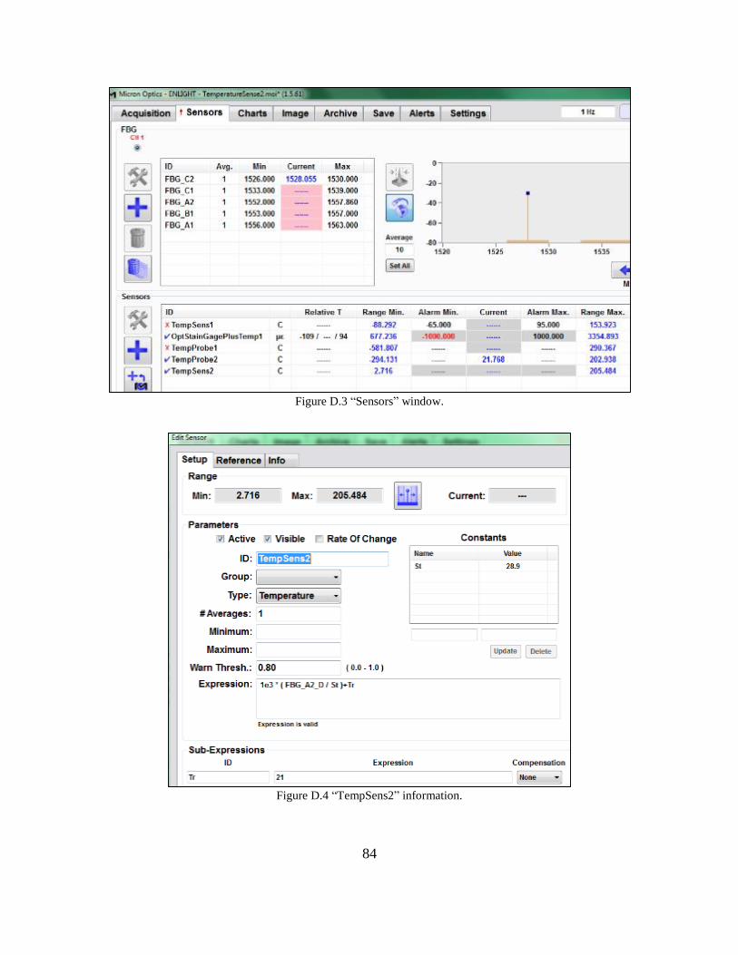
84

Figure D.3 “Sensors” window.

Figure D.4 “TempSens2” information.

85

Figure D.5 “TempProbe2” information.

Figure D.6 Charts window with live temperature data.

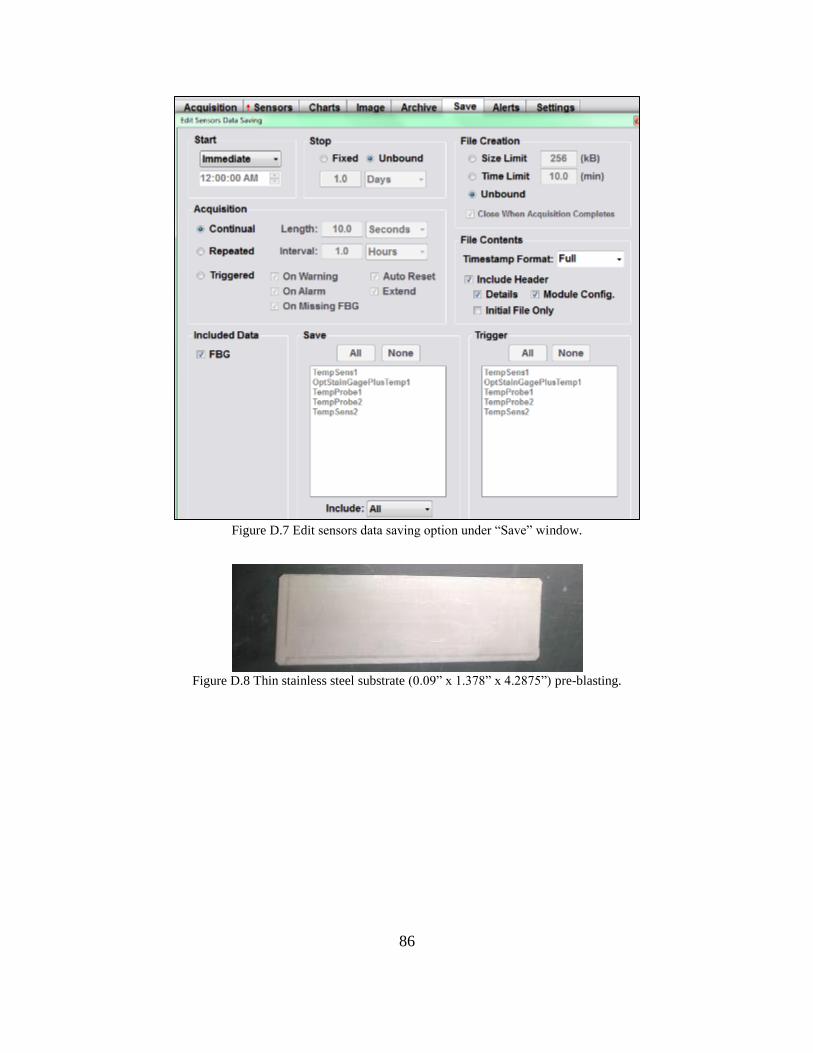
86

Figure D.7 Edit sensors data saving option under “Save” window.

Figure D.8 Thin stainless steel substrate (0.09” x 1.378” x 4.2875”) pre-blasting.

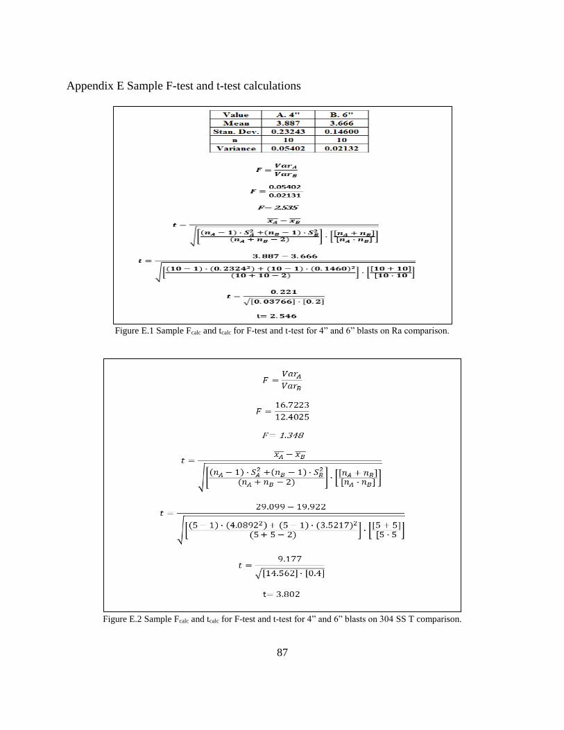
87

Appendix E Sample F-test and t-test calculations

Figure E.1 Sample Fcalc and tcalc for F-test and t-test for 4” and 6” blasts on Ra comparison.

Figure E.2 Sample Fcalc and tcalc for F-test and t-test for 4” and 6” blasts on 304 SS T comparison.

88

89

Appendix F Roughness F-tests and t-tests Data

Figure F.1 F-test and t-test results for 4” and 6” blasts on Ra comparison.

Figure F.2 F-test and t-test results for 6” and 8” Ra comparison.

Figure F.3 F-test and t-test results for 42 psi and 60 psi Ra comparison.

Data 1. 4" 2. 6"

Ra #1 3.77 3.96

Ra #2 3.8 3.52 Variable 1 Variable 2 Variable 1 Variable 2

Ra #3 3.96 3.75 Mean 3.887 3.668 Mean 3.887 3.668

Ra #4 3.81 3.53 Variance 0.0540 0.0216 Variance 0.0540 0.0216

Ra #5 3.8 3.64 Observations 10 10 Observations 10 10

Ra #6 3.78 3.5 df 9 9 Pooled Variance 0.0378

Ra #7 4.52 3.72 F 2.496 Hypothesized Mean Diff. 0

Ra #8 3.72 3.7 P(F<=f) one-tail 0.0946 df 18

Ra #9 3.9 3.56 F Critical one-tail 3.179 t Stat 2.518

Ra #10 3.81 3.8 P(T<=t) two-tail 0.0215

t Critical two-tail 2.101Standard

Deviation0.232 0.147

Standard

Error0.0735 0.0465

Variances are equal.

F-Test Two-Sample for Variances t-Test: Two-Sample Assuming Equal Variances

Fcalc < Fcritical

Data 2. 6" 3. 8"

Ra #1 3.96 3.41

Ra #2 3.52 3.45 Variable 1 Variable 2 Variable 1 Variable 2

Ra #3 3.75 3.34 Mean 3.668 3.446 Mean 3.668 3.446

Ra #4 3.53 3.24 Variance 0.0216 0.0188 Variance 0.0216 0.0188

Ra #5 3.64 3.6 Observations 10 10 Observations 10 10

Ra #6 3.5 3.7 df 9 9 Pooled Variance 0.0202

Ra #7 3.72 3.52 F 1.148 Hypothesized Mean Diff. 0

Ra #8 3.7 3.48 P(F<=f) one-tail 0.420 df 18

Ra #9 3.56 3.31 F Critical one-tail 3.179 t Stat 3.489

Ra #10 3.8 3.41 P(T<=t) two-tail 0.00262

t Critical two-tail 2.101

t-Test: Two-Sample Assuming Equal VariancesF-Test Two-Sample for Variances

Standard

Deviation0.147 0.137

Standard

Error0.0465 0.0434

Variances are equal.

Fcalc < Fcritical

Data 9. 42 psi 10. 60 psi

Ra #1 5.07 4.81

Ra #2 5.19 4.65 Variable 1 Variable 2 Variable 1 Variable 2

Ra #3 5.33 4.72 Mean 5.012 4.675 Mean 5.012 4.675

Ra #4 5.37 4.98 Variance 0.0566 0.0407 Variance 0.0566 0.0407

Ra #5 4.99 4.45 Observations 10 10 Observations 10 10

Ra #6 4.74 4.86 df 9 9 Pooled Variance 0.0486

Ra #7 4.82 4.61 F 1.391 Hypothesized Mean Diff. 0

Ra #8 4.77 4.84 P(F<=f) one-tail 0.315 df 18

Ra #9 4.75 4.43 F Critical one-tail 3.179 t Stat 3.418

Ra #10 5.09 4.4 P(T<=t) two-tail 0.00307

t Critical two-tail 2.101

F-Test Two-Sample for Variances

F calc < Fcritical

Variances are equal.

t-Test: Two-Sample Assuming Equal Variances

Standard

Deviation0.238 0.202

Standard

Error0.0752 0.0638

90

Figure F.4 F-test and t-test results for 5/16” straight and 3/16” Venturi nozzle Ra comparison.

Figure F.5 F-test and t-test results for no pulsation and pulsation Ra comparison.

Figure F.6 F-test and t-test results for newer media and old (recycled media) Ra comparison.

Data 6. 5/16" Straight 18. 3/16" Venturi

Ra #1 4.16 4.64

Ra #2 4.33 4.23 Variable 1 Variable 2 Variable 1 Variable 2

Ra #3 4.46 4.19 Mean 4.234 4.24 Mean 4.24 4.234

Ra #4 4.29 4.41 Variance 0.0572 0.0121 Variance 0.0121 0.0572

Ra #5 4.07 4.54 Observations 10 10 Observations 10 10

Ra #6 4.27 4.23 df 9 9 Hypothesized Mean Diff. 0

Ra #7 4.15 3.92 F 4.721 df 13

Ra #8 4.20 4.14 P(F<=f) one-tail 0.0151 t Stat 0.0721

Ra #9 4.28 4.13 F Critical one-tail 3.179 P(T<=t) two-tail 0.944

Ra #10 4.19 3.91 t Critical two-tail 2.160

F-Test Two-Sample for Variances

F calc > Fcritical

Variances are not equal.

t-Test: Two-Sample Assuming Unequal Variances

Standard

Deviation0.110 0.239

Standard

Error0.0348 0.0756

Data 18. No Pulsation 2. Pulsation

Ra #1 4.64 3.96

Ra #2 4.23 3.52 Variable 1 Variable 2 Variable 1 Variable 2

Ra #3 4.19 3.75 Mean 4.234 3.668 Mean 4.234 3.668

Ra #4 4.41 3.53 Variance 0.0572 0.0216 Variance 0.0572 0.0216

Ra #5 4.54 3.64 Observations 10 10 Observations 10 10

Ra #6 4.23 3.5 df 9 9 Pooled Variance 0.0394

Ra #7 3.92 3.72 F 2.642 Hypothesized Mean Diff. 0

Ra #8 4.14 3.7 P(F<=f) one-tail 0.0820 df 18

Ra #9 4.13 3.56 F Critical one-tail 3.179 t Stat 6.375

Ra #10 3.91 3.8 P(T<=t) two-tail 5.275E-06

t Critical two-tail 2.101Standard

Deviation0.239 0.147

Standard

Error0.0756 0.0465

F-Test Two-Sample for Variances

Variances are equal.

t-Test: Two-Sample Assuming Equal Variances

F calc < Fcritical

Data 13. Old 18. New

Ra #1 5.12 4.64

Ra #2 5.07 4.23 Variable 1 Variable 2 Variable 1 Variable 2

Ra #3 4.61 4.19 Mean 4.697 4.234 Mean 4.697 4.234

Ra #4 4.79 4.41 Variance 0.0580 0.0572 Variance 0.0580 0.0572

Ra #5 4.63 4.54 Observations 10 10 Observations 10 10

Ra #6 4.6 4.23 df 9 9 Pooled Variance 0.0576

Ra #7 4.52 3.92 F 1.014 Hypothesized Mean Diff. 0

Ra #8 4.33 4.14 P(F<=f) one-tail 0.492 df 18

Ra #9 4.61 4.13 F Critical one-tail 3.179 t Stat 4.314

Ra #10 4.69 3.91 P(T<=t) two-tail 0.000417

t Critical two-tail 2.101

t-Test: Two-Sample Assuming Equal Variances

Standard

Error0.0761 0.0756

F-Test Two-Sample for Variances

Variances are equal.

F calc < Fcritical

Standard

Deviation0.241 0.239

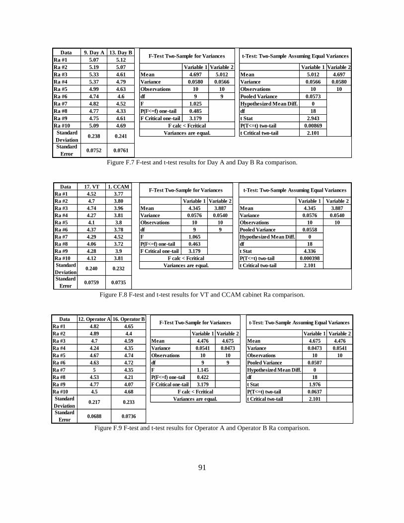
91

Figure F.7 F-test and t-test results for Day A and Day B Ra comparison.

Figure F.8 F-test and t-test results for VT and CCAM cabinet Ra comparison.

Figure F.9 F-test and t-test results for Operator A and Operator B Ra comparison.

Data 9. Day A 13. Day B

Ra #1 5.07 5.12

Ra #2 5.19 5.07 Variable 1 Variable 2 Variable 1 Variable 2

Ra #3 5.33 4.61 Mean 4.697 5.012 Mean 5.012 4.697

Ra #4 5.37 4.79 Variance 0.0580 0.0566 Variance 0.0566 0.0580

Ra #5 4.99 4.63 Observations 10 10 Observations 10 10

Ra #6 4.74 4.6 df 9 9 Pooled Variance 0.0573

Ra #7 4.82 4.52 F 1.025 Hypothesized Mean Diff. 0

Ra #8 4.77 4.33 P(F<=f) one-tail 0.485 df 18

Ra #9 4.75 4.61 F Critical one-tail 3.179 t Stat 2.943

Ra #10 5.09 4.69 P(T<=t) two-tail 0.00869

t Critical two-tail 2.101Standard

Deviation0.238 0.241

Standard

Error0.0752 0.0761

F calc < Fcritical

Variances are equal.

F-Test Two-Sample for Variances t-Test: Two-Sample Assuming Equal Variances

Data 17. VT 1. CCAM

Ra #1 4.52 3.77

Ra #2 4.7 3.80 Variable 1 Variable 2 Variable 1 Variable 2

Ra #3 4.74 3.96 Mean 4.345 3.887 Mean 4.345 3.887

Ra #4 4.27 3.81 Variance 0.0576 0.0540 Variance 0.0576 0.0540

Ra #5 4.1 3.8 Observations 10 10 Observations 10 10

Ra #6 4.37 3.78 df 9 9 Pooled Variance 0.0558

Ra #7 4.29 4.52 F 1.065 Hypothesized Mean Diff. 0

Ra #8 4.06 3.72 P(F<=f) one-tail 0.463 df 18

Ra #9 4.28 3.9 F Critical one-tail 3.179 t Stat 4.336

Ra #10 4.12 3.81 P(T<=t) two-tail 0.000398

t Critical two-tail 2.101Standard

Deviation0.240 0.232

Standard

Error0.0759 0.0735

F-Test Two-Sample for Variances

F calc < Fcritical

Variances are equal.

t-Test: Two-Sample Assuming Equal Variances

Data 12. Operator A 16. Operator B

Ra #1 4.82 4.65

Ra #2 4.89 4.4 Variable 1 Variable 2 Variable 1 Variable 2

Ra #3 4.7 4.59 Mean 4.476 4.675 Mean 4.675 4.476

Ra #4 4.24 4.35 Variance 0.0541 0.0473 Variance 0.0473 0.0541

Ra #5 4.67 4.74 Observations 10 10 Observations 10 10

Ra #6 4.63 4.72 df 9 9 Pooled Variance 0.0507

Ra #7 5 4.35 F 1.145 Hypothesized Mean Diff. 0

Ra #8 4.53 4.21 P(F<=f) one-tail 0.422 df 18

Ra #9 4.77 4.07 F Critical one-tail 3.179 t Stat 1.976

Ra #10 4.5 4.68 P(T<=t) two-tail 0.0637

t Critical two-tail 2.101Standard

Deviation0.217 0.233

Standard

Error0.0688 0.0736

F-Test Two-Sample for Variances

F calc < Fcritical

Variances are equal.

t-Test: Two-Sample Assuming Equal Variances

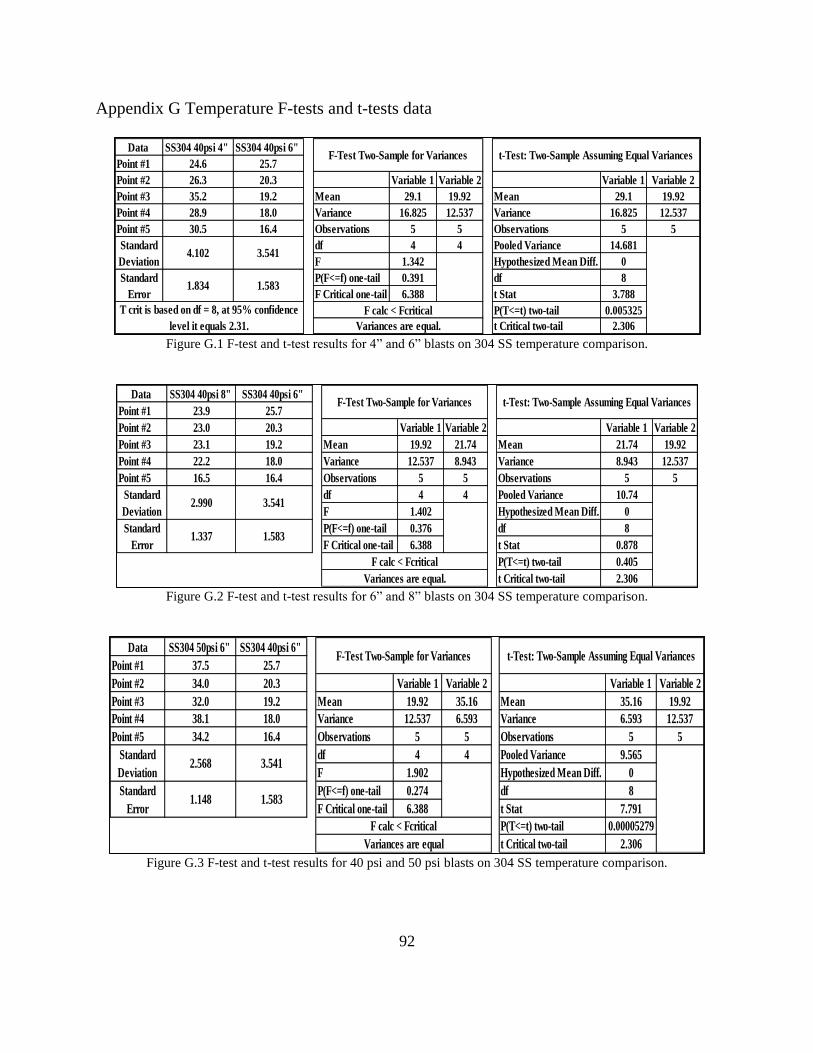
92

Appendix G Temperature F-tests and t-tests data

Figure G.1 F-test and t-test results for 4” and 6” blasts on 304 SS temperature comparison.

Figure G.2 F-test and t-test results for 6” and 8” blasts on 304 SS temperature comparison.

Figure G.3 F-test and t-test results for 40 psi and 50 psi blasts on 304 SS temperature comparison.

Data SS304 40psi 4" SS304 40psi 6"

Point #1 24.6 25.7

Point #2 26.3 20.3 Variable 1 Variable 2 Variable 1 Variable 2

Point #3 35.2 19.2 Mean 29.1 19.92 Mean 29.1 19.92

Point #4 28.9 18.0 Variance 16.825 12.537 Variance 16.825 12.537

Point #5 30.5 16.4 Observations 5 5 Observations 5 5

df 4 4 Pooled Variance 14.681

F 1.342 Hypothesized Mean Diff. 0

P(F<=f) one-tail 0.391 df 8

F Critical one-tail 6.388 t Stat 3.788

P(T<=t) two-tail 0.005325

t Critical two-tail 2.306

T crit is based on df = 8, at 95% confidence

level it equals 2.31.

F-Test Two-Sample for Variances t-Test: Two-Sample Assuming Equal Variances

F calc < Fcritical

Variances are equal.

Standard

Deviation4.102 3.541

Standard

Error1.834 1.583

Data SS304 40psi 8" SS304 40psi 6"

Point #1 23.9 25.7

Point #2 23.0 20.3 Variable 1 Variable 2 Variable 1 Variable 2

Point #3 23.1 19.2 Mean 19.92 21.74 Mean 21.74 19.92

Point #4 22.2 18.0 Variance 12.537 8.943 Variance 8.943 12.537

Point #5 16.5 16.4 Observations 5 5 Observations 5 5

df 4 4 Pooled Variance 10.74

F 1.402 Hypothesized Mean Diff. 0

P(F<=f) one-tail 0.376 df 8

F Critical one-tail 6.388 t Stat 0.878

P(T<=t) two-tail 0.405

t Critical two-tail 2.306

Standard

Deviation2.990 3.541

Standard

Error1.337 1.583

F-Test Two-Sample for Variances t-Test: Two-Sample Assuming Equal Variances

F calc < Fcritical

Variances are equal.

Data SS304 50psi 6" SS304 40psi 6"

Point #1 37.5 25.7

Point #2 34.0 20.3 Variable 1 Variable 2 Variable 1 Variable 2

Point #3 32.0 19.2 Mean 19.92 35.16 Mean 35.16 19.92

Point #4 38.1 18.0 Variance 12.537 6.593 Variance 6.593 12.537

Point #5 34.2 16.4 Observations 5 5 Observations 5 5

df 4 4 Pooled Variance 9.565

F 1.902 Hypothesized Mean Diff. 0

P(F<=f) one-tail 0.274 df 8

F Critical one-tail 6.388 t Stat 7.791

P(T<=t) two-tail 0.00005279

t Critical two-tail 2.306

F-Test Two-Sample for Variances t-Test: Two-Sample Assuming Equal Variances

Standard

Deviation2.568 3.541

Standard

Error1.148 1.583

F calc < Fcritical

Variances are equal

93

Figure G.4 F-test and t-test results for 50 psi and 60psi blasts on 304 SS temperature comparison.

Figure G.5 F-test and t-test results for 45°and 90° blasts on 304 SS temperature comparison.

Figure G.6 F-test and t-test results for 6” and 8” blasts on thin SS temperature comparison.

Data SS304 60psi 6" SS304 50psi 6"

Point #1 49.5 37.5

Point #2 38.7 34 Variable 1 Variable 2 Variable 1 Variable 2

Point #3 44.8 32 Mean 45.08 35.16 Mean 45.08 35.16

Point #4 42.2 38.1 Variance 23.707 6.593 Variance 23.707 6.593

Point #5 50.2 34.2 Observations 5 5 Observations 5 5

df 4 4 Pooled Variance 15.15

F 3.596 Hypothesized Mean Diff. 0

P(F<=f) one-tail 0.121 df 8

F Critical one-tail 6.388 t Stat 4.030

P(T<=t) two-tail 0.003790

t Critical two-tail 2.306

Standard

Deviation4.869 2.568

Standard

Error2.177 1.148

F-Test Two-Sample for Variances

Variances are equal

t-Test: Two-Sample Assuming Equal Variances

F calc < Fcritical

Data SS304 90° SS304 45°Point #1 25.7 7.9

Point #2 20.3 7.7 Variable 1 Variable 2 Variable 1 Variable 2

Point #3 19.2 7.6 Mean 19.92 8.3 Mean 19.92 8.3

Point #4 18 8.4 Variance 12.537 0.895 Variance 12.537 0.895

Point #5 16.4 9.9 Observations 5 5 Observations 5 5

df 4 4 Hypothesized Mean Diff. 0

F 14.008 df 5

P(F<=f) one-tail 0.01273 t Stat 7.090

F Critical one-tail 6.388 P(T<=t) two-tail 0.0008646

t Critical two-tail 2.571

Standard

Deviation 3.541 0.946

Standard

Error1.583 0.423

F-Test Two-Sample for Variances

Fcalc > Fcrit

Variances are unequal

t-Test: Two-Sample Assuming Unequal Variances

Data SSThin 40psi 6" SSThin 40psi 8"

Point #1 26.8 16.4

Point #2 20.3 15.6 Variable 1 Variable 2 Variable 1 Variable 2

Point #3 30.8 13.3 Mean 24.14 14.3 Mean 24.14 14.3

Point #4 22 12.3 Variance 20.478 2.815 Variance 20.478 2.815

Point #5 20.8 13.9 Observations 5 5 Observations 5 5

df 4 4 Hypothesized Mean Diff. 0

F 7.275 df 5

P(F<=f) one-tail 0.04029 t Stat 4.559

F Critical one-tail 6.388 P(T<=t) two-tail 0.006063

t Critical two-tail 2.571T crit is based on df = 5, at 95% confidence

level it equals 2.57.

F calc > Fcritical

Variances are not Equal

Standard

Error2.024 0.750

Standard

Deviation 4.525 1.678

t-Test: Two-Sample Assuming Unequal VariancesF-Test Two-Sample for Variances

94

Figure G.7 F-test and t-test results for 40 psi and 60 psi blasts on thin SS temperature comparison.

Figure G.8 F-test and t-test results for 45°and 90° blasts on thin SS temperature comparison.

Figure G.9 F-test and t-test results for 6”, 40 psi blasts of both substrates for T comparison.

Data SSThin 60psi 6" SSThin 40psi 6"

Point #1 32.6 26.8

Point #2 27.3 20.3 Variable 1 Variable 2 Variable 1 Variable 2

Point #3 23.2 30.8 Mean 24.92 24.14 Mean 24.92 24.14

Point #4 21.4 22 Variance 25.807 20.478 Variance 25.807 20.478

Point #5 20.1 20.8 Observations 5 5 Observations 5 5

df 4 4 Pooled Variance 23.1425

F 1.260 Hypothesized Mean Diff. 0

P(F<=f) one-tail 0.414 df 8

F Critical one-tail 6.388 t Stat 0.256

P(T<=t) two-tail 0.804

t Critical two-tail 2.306Variances are equal

t-Test: Two-Sample Assuming Equal VariancesF-Test Two-Sample for Variances

F calc < Fcritical

Standard

Deviation 5.080 4.525

Standard

Error2.272 2.024

Data SSThin 40psi 6" SSThin 40psi 6" 45°

Point #1 26.8 23.6

Point #2 20.3 20.9 Variable 1 Variable 2 Variable 1 Variable 2

Point #3 30.8 23.4 Mean 24.14 23.52 Mean 24.14 23.52

Point #4 22 27.3 Variance 20.478 5.607 Variance 20.478 5.607

Point #5 20.8 22.4 Observations 5 5 Observations 5 5

df 4 4 Pooled Variance 13.0425

F 3.652 Hypothesized Mean Diff. 0

P(F<=f) one-tail 0.119 df 8

F Critical one-tail 6.388 t Stat 0.271

P(T<=t) two-tail 0.793

t Critical two-tail 2.306

Standard

Deviation 4.525 2.368

Standard

Error2.024 1.059

F-Test Two-Sample for Variances t-Test: Two-Sample Assuming Equal Variances

F calc < Fcritical

Variances are equal.

Data SSThin 40psi 6" SS304 40psi 6"

Point #1 26.8 25.7

Point #2 20.3 20.3 Variable 1 Variable 2 Variable 1 Variable 2

Point #3 30.8 19.2 Mean 24.14 19.92 Mean 24.14 19.92

Point #4 22 18 Variance 20.478 12.537 Variance 20.478 12.537

Point #5 20.8 16.4 Observations 5 5 Observations 5 5

df 4 4 Pooled Variance 16.5075

F 1.633 Hypothesized Mean Diff. 0

P(F<=f) one-tail 0.323 df 8

F Critical one-tail 6.388 t Stat 1.642

P(T<=t) two-tail 0.139

t Critical two-tail 2.306Variances are equal.

Standard

Deviation 4.525

Standard

Error2.024

3.541

1.583

F-Test Two-Sample for Variances t-Test: Two-Sample Assuming Equal Variances

F calc < Fcritical

95

Figure G.10 F-test and t-test results for 8”, 40 psi blasts of both substrates for T comparison.

Figure G.11 F-test and t-test results for 6”, 60 psi blasts of both substrates for T comparison.

Figure G.12 F-test and t-test results for 45°, 40 psi blasts of both substrates for T comparison.

Data SS304 40psi 8" SSThin 40psi 8"

Point #1 23.9 16.4

Point #2 23 15.6 Variable 1 Variable 2 Variable 1 Variable 2

Point #3 23.1 13.3 Mean 21.74 14.3 Mean 21.74 14.3

Point #4 22.2 12.3 Variance 8.943 2.815 Variance 8.943 2.815

Point #5 16.5 13.9 Observations 5 5 Observations 5 5

df 4 4 Pooled Variance 5.879

F 3.177 Hypothesized Mean Diff. 0

P(F<=f) one-tail 0.145 df 8

F Critical one-tail 6.388 t Stat 4.852

P(T<=t) two-tail 0.001269

t Critical two-tail 2.306

F-Test Two-Sample for Variances t-Test: Two-Sample Assuming Equal Variances

F calc < Fcritical

Standard

Deviation 2.990 1.678

Standard

Error1.337 0.750

Variances are equal.

Data SS304 60psi 6" SSThin 60psi 6"

Point #1 49.5 32.6

Point #2 38.7 27.3 Variable 1 Variable 2 Variable 1 Variable 2

Point #3 44.8 23.2 Mean 24.92 45.08 Mean 45.08 24.92

Point #4 42.2 21.4 Variance 25.807 23.707 Variance 23.707 25.807

Point #5 50.2 20.1 Observations 5 5 Observations 5 5

df 4 4 Pooled Variance 24.757

F 1.089 Hypothesized Mean Diff. 0

P(F<=f) one-tail 0.468 df 8

F Critical one-tail 6.388 t Stat 6.406

P(T<=t) two-tail 0.0002077

t Critical two-tail 2.306

Standard

Deviation 4.869 5.080

Standard

Error2.177 2.272

Variances are equal.

F-Test Two-Sample for Variances t-Test: Two-Sample Assuming Equal Variances

F calc < Fcritical

Data SSThin 40psi 6" 45° SS304 40psi 6" 45°

Point #1 23.6 7.9

Point #2 20.9 7.7 Variable 1 Variable 2 Variable 1 Variable 2

Point #3 23.4 7.6 Mean 23.52 8.3 Mean 23.52 8.3

Point #4 27.3 8.4 Variance 5.607 0.895 Variance 5.607 0.895

Point #5 22.4 9.9 Observations 5 5 Observations 5 5

df 4 4 Pooled Variance 3.251

F 6.265 Hypothesized Mean Diff. 0

P(F<=f) one-tail 0.0516 df 8

F Critical one-tail 6.388 t Stat 13.347

P(T<=t) two-tail 9.495 x 10-7

t Critical two-tail 2.306

F-Test Two-Sample for Variances

Variances are equal.

t-Test: Two-Sample Assuming Equal Variances

F calc < Fcritical

Standard

Deviation

Standard

Error1.057 0.420

2.368 0.946

96

Appendix H Figures and Tables Permissions

Figure 2.1 [2, used with permission]

No Author. “Technical Reference: Surface Preparation.” Blast One. 2014. http://www.blast-

one.com/weekly-tips/the-difference-between-surface-profile-and-class-of-blast (accessed May

14, 2014) Used with permission from Blast One; email attached.

Table 2-1 [5, used with permission]

Momber A. Blast Cleaning Technology: Chapter 1: Introduction, 2008. p. 3.

http://vt.summon.serialssolutions.com/link/0/eLvHCXMwY2BQSDK1MDBNTgFmnETTFHNg

g98C2OpIArZdjUxSk9PSTFB2vCOV5m6iDGZuriHOHrqwOcn4AsiRC_GISXxz0LyZrimwyQ

qsWE3iQav0jQzFGHgTQQvC80rAG8dS-JI4LvXUxfgmLD09V8ppeRo3AOU_KUc (accessed

March 31, 2013) Used with permission from Copyright Clearance Center; letter attached.

Figure 2.2 [6, used with permission]

No Author. “Blast Cabinets.” Norton Sandblasting Equipment, 2014. Date Obtained: May 14,

2014. Online: http://www.nortonsandblasting.com/nsbcontact.html (accessed May 14, 2014) Used

with permission from Norton Sandblasting Equipment; email attached.

Figure 2.3 [8, used with permission]

Momber A. Blast Cleaning Technology: Chapter 2: Abrasive Materials, 2008. p. 19.

http://link.springer.com/chapter/10.1007%2F978-3-540-73645-5_2 (accessed March 31, 2013)

Used with permission from Copyright Clearance Center; letter attached.

Figure 2.4 [11, 12 used with permission]

Momber A. Blast Cleaning Technology: Chapter 2: Abrasive Materials, 2008. p. 21.

http://link.springer.com/chapter/10.1007%2F978-3-540-73645-5_2 (accessed March 31, 2013)

Used with permission from Copyright Clearance Center; letter attached.

Figure 2.5 [14, used with permission]

Momber A. Blast Cleaning Technology: Chapter 2: Abrasive Materials, 2008. p. 20.

http://link.springer.com/chapter/10.1007%2F978-3-540-73645-5_2 (accessed March 31, 2013)

Used with permission from Copyright Clearance Center; letter attached.

Figure 2.6 [15, used with permission]

Momber A. Blast Cleaning Technology: Chapter 2: Abrasive Materials, 2008. p. 18.

http://link.springer.com/chapter/10.1007%2F978-3-540-73645-5_2 (accessed March 31, 2013)

Used with permission from Copyright Clearance Center; letter attached.

Figure 2.7 [18, used with permission]

Momber A. Blast Cleaning Technology: Chapter 2: Abrasive Materials, 2008. p. 26.

http://link.springer.com/chapter/10.1007%2F978-3-540-73645-5_2 (accessed March 31, 2013)

Used with permission from Copyright Clearance Center; letter attached.

Figure 2.8 [23, used with permission]

Day, James; Huang, Xiao; and Richards, N.L. “Examination of a Grit-Blasting Process for

Thermal Spraying Using Statistical Methods.” Journal of Thermal Spray Technology, 2005/Vol.

97

14, p. 477. http://link.springer.com/article/10.1361%2F105996305X76469 (accessed November

2012) Used with permission from Copyright Clearance Center; letter attached.

Figure 2.9 [24, used with permission]

Maruyama T, Akagi K, Kobayashi T. "Effects of Blasting Parameters on Removability of Residual

Grit." Journal of Thermal Spray Technology. 2006/Vol. 15, no. 4. p. 820.

http://link.springer.com/article/10.1361%2F105996306X147018 (accessed November 2, 2012)

Used with permission from Copyright Clearance Center; letter attached.

Table 2-2 [27, used with permission]

Momber A. Blast Cleaning Technology: Chapter 2: Abrasive Materials, 2008. p. 14.

http://link.springer.com/chapter/10.1007%2F978-3-540-73645-5_2 (accessed April 1, 2013)

Used with permission from Copyright Clearance Center; letter attached.

Figure 2.10 [34, used with permission]

Momber A. Blast Cleaning Technology: Chapter 6: Surface Preparation Process, 2008. p. 280.

http://link.springer.com/chapter/10.1007/978-3-540-73645-5_6 (accessed March 31, 2013) Used

with permission from Copyright Clearance Center; letter attached.

Figure 2.11 [36, used with permission]

Makova, I., Sopko, M. "Effect of Blasting Material on Surface Morphology of Steel Sheets."

Acta Metallurgica Slovaca. 2010/ Vol. 16, no. 2, p. 111. (accessed March 07, 2013) Used with

permission from Act Metallurgica Slovaca; email attached.

Figure 2.12 [38, 39 used with permission]

Momber A. Blast Cleaning Technology: Chapter 2: Abrasive Materials, 2008. p. 11, 12.

http://link.springer.com/chapter/10.1007%2F978-3-540-73645-5_2 (accessed March 31, 2013)

Used with permission from Copyright Clearance Center; letter attached.

Figure 2.13 [50, used with permission]

Fang, C.K., Chuang, T.H. "Erosion of SS41 Steel by Sand Blasting." Metallurgical and Materials

Transactions A. 1999/Vol. 30A, p. 944. (accessed January 11, 2013) Used with permission from

Copyright Clearance Center; letter attached.

Figure 2.14 [50, used with permission]

Fang, C.K., Chuang, T.H. "Erosion of SS41 Steel by Sand Blasting." Metallurgical and Materials

Transactions A. 1999/Vol. 30A, p. 944. (accessed January 11, 2013) Used with permission from

Copyright Clearance Center; letter attached.

Figure 2.15 [51, used with permission]

Mellalia, M., Grimaud, A., Leger, A.C., Fauchais, P., and Lu, J. “Alumina Grit Blasting Parameters

for Surface Preparation in the Plasma Spraying Operation.” Journal of Thermal Spray Technology.

1997/Vol 6. No. 2. p 219. (accessed October 22, 2012) Used with permission from Copyright

Clearance Center; letter attached.

98

Figure 2.16 [53, used with permission]

Chander, K. Poorna, Vashita, M., Sabiruddin, Kazi, Paul, S., Bandyopadhyay, P.P. “Effects of

Grit Blasting on Surface Properties of Steel Substrates.” Materials and Design. 2009. p. 2901.

(accessed November 2012) Used with permission from Copyright Clearance Center; letter

attached.

Figure 2.17 [53, used with permission]

Chander, K. Poorna, Vashita, M., Sabiruddin, Kazi, Paul, S., Bandyopadhyay, P.P. “Effects of

Grit Blasting on Surface Properties of Steel Substrates.” Materials and Design. 2009. p. 2899.

(accessed November 2012) Used with permission from Copyright Clearance Center; letter

attached.

Figure 2.18 [51, used with permission]

Mellalia, M., Grimaud, A., Leger, A.C., Fauchais, P., and Lu, J. “Alumina Grit Blasting Parameters

for Surface Preparation in the Plasma Spraying Operation.” Journal of Thermal Spray Technology.

1997/Vol 6. No. 2. p 221. (accessed October 22, 2012) Used with permission from Copyright

Clearance Center; letter attached.

Figure 2.19 [54, used with permission]

Amada, Shigeyasu, Hirose, Tohru. "Influence of grit blasting pre-treatment on the adhesion

strength of plasma sprayed coatings: fractal analysis of roughness." Surface and Coatings

Technology. 1998/Vol. 102. p. 134. http://dx.doi.org/10.1016/S0257-8972(97)00628-2 (accessed

October 29, 2012) Used with permission from Copyright Clearance Center; letter attached.

Figure 2.20 [55, used with permission]

Carter, G., Bevan I.J., Katardjiev I.V., Nobes, M.J. "The Erosion of Copper by Reflected

Sandblasting Grains." Materials Science Engineering. 1991/Vol. A. no. 132. P. 232. (accessed

October 22, 2012) Used with permission from Copyright Clearance Center; letter attached.

Figure 2.21 [56, used with permission]

Celik, E., Demirkiran, A.S., Avci, E. "Effect of Grit Blasting of Substrate on the Corrosion

Behaviour of Plasma-Sprayed Al2O3 Coatings." Surface and Coatings Technology. 1999/Vol.

116-119. p. 1062. (accessed October 29, 2012) Used with permission from Copyright Clearance

Center; letter attached.

Figure 2.22 [59, used with permission]

Wigren, Jan. "Technical Note: Grit Blasting as Surface Preparation Before Plasma Spraying."

Surface and Coatings Technology. 1988/Vol 34. p. 107. (accessed January 15, 2013) Used with

permission from Copyright Clearance Center; letter attached.

Figure 2.23 [60, used with permission]

Momber A. Blast Cleaning Technology: Chapter 2: Abrasive Materials, 2008. p. 38.

http://link.springer.com/chapter/10.1007%2F978-3-540-73645-5_2 (accessed March 31, 2013)

Used with permission from Copyright Clearance Center; letter attached.

Figure 2.24 [62, used with permission]

99

Momber A. Blast Cleaning Technology: Chapter 2: Abrasive Materials, 2008. p. 47, 48.

http://link.springer.com/chapter/10.1007%2F978-3-540-73645-5_2 (accessed March 31, 2013)

Used with permission from Copyright Clearance Center; letter attached.

Figure 2.25 [64, used with permission]

Tabenkin, Alex. “The Basics of Surface Finish Measurement.” Quality Magazine. 2014.

http://www.deterco.com/products/Mahr%20Federal/newsletter/finish_measure_10_19_04.htm

(accessed May 14, 2014) Used with permission from Mahr Federal Inc.; email attached.

Figure 2.26 [66, used with permission]

Pickrell, G., Homa, D, Mills, R. “Abrasive Blasting Deliverable No.3.” CCAM. 2014. (accessed

April 2, 2014) Used with permission from Robert Mills.

Figure 2.27 [67, used with permission]

Sosale, G., Hackling S.A., and Vengallatore, S. "Topography Analysis of Grit-Blasted and Grit-

Blasted-Acid Etched Titanium Implant Surfaces Using Multi-scale Measurements and Multi-

Parameter Statistics." Journal of Materials Research. 2011/Vol. 23, Issue 10. p. 2709. (accessed

June 6, 2014) Used with permission from Copyright Clearance Center; letter attached.

Table A-1 [35, used with permission]

No Author. “Blast Media Chart.” Norton Sandblasting Equipment. 2014.

http://www.nortonsandblasting.com/nsbabrasives.html (accessed June 9, 2014) Used with

permission from Norton Sandblasting Equipment; email attached.

Figure B.1 [63, used with permission]

No Author. “Abrasive Blast Nozzles.” Kennametal Inc. 2012 page 9.

http://www.kennametal.com/content/dam/kennametal/kennametal/common/Resources/Catalogs-

Literature/Advanced%20Materials%20and%20Wear%20Components/B-12-

02861_KMT_Blast_Nozzles_Catalog_EN.pdf (accessed June 9, 2014) Used with permission

from Kennametal, Inc.; email attached.