Physical modeling of atmospheric boundary layer flows Part I: Overview of modeling concepts and techniques

Part II: Modeling neutrally stratified boundary layer flows Evgeni Fedorovich

School of Meteorology, University of Oklahoma, Norman, USA

Outline • Place of physical modeling in the triad of approaches to study

atmospheric boundary layer flows • Concept of physical modeling: prototype versus model • Commonly employed laboratory facilities and techniques • Wind tunnel modeling of neutrally stratified boundary layers • Methodology of generating neutral boundary layer flows in wind tunnels • Review of turbulent flow properties over rough and smooth surfaces • Similarity requirements; comparisons with atmospheric data • Tracer dispersion from a line source: numerical model evaluation

• Summarizing remarks

Triad of approaches in atmospheric boundary layer studies

I. Field observations/measurements • In situ/contact measurements

• Remote sensing techniques

II. Physical/laboratory models • Laboratory tank (thermal and saline) models

• Water channel/tunnel/flume models

• Wind tunnel (stratified and neutral) models

III. Theoretical/numerical techniques • Theoretical/analytical models

• Numerical models/parameterizations

• Numerical simulations (direct and large-eddy)

I. Field observations/measurements In situ/contact measurements and remote sensing techniques

Single global asset: it is real!

Hard or impossible to • separate different contributing forcings/mechanisms • match temporal/spatial requirements for retrieval of statistics • control external forcings and boundary conditions • obtain accurate and complete data at low cost

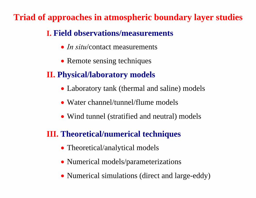
II. Physical/laboratory models Laboratory tanks, water channels, wind tunnels

Pros: • High level of complexity of

modeled flows • Controlled external/boundary

parameters • Repeatability of flow regimes • Possibility to generate well-

documented data sets for evaluation of numerical models/simulations

Hard or impossible to • reproduce several contributing

forcings in combination • sufficiently match scaling/similarity

requirements in order to relate the modeled flow to its atmospheric prototype

• find a reasonable balance between the value of results and cost of facility

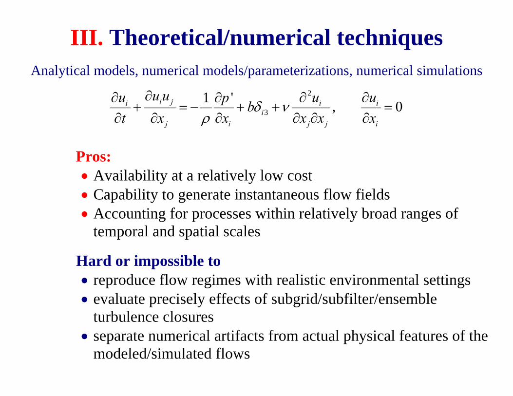
III. Theoretical/numerical techniques Analytical models, numerical models/parameterizations, numerical simulations

2

31 ' , 0i ji i i

ij i j j i

u uu u up bt x x x x x

δ νρ

∂∂ ∂ ∂∂+ = − + + =

∂ ∂ ∂ ∂ ∂ ∂

Pros: • Availability at a relatively low cost • Capability to generate instantaneous flow fields • Accounting for processes within relatively broad ranges of

temporal and spatial scales

Hard or impossible to • reproduce flow regimes with realistic environmental settings • evaluate precisely effects of subgrid/subfilter/ensemble

turbulence closures • separate numerical artifacts from actual physical features of the

modeled/simulated flows

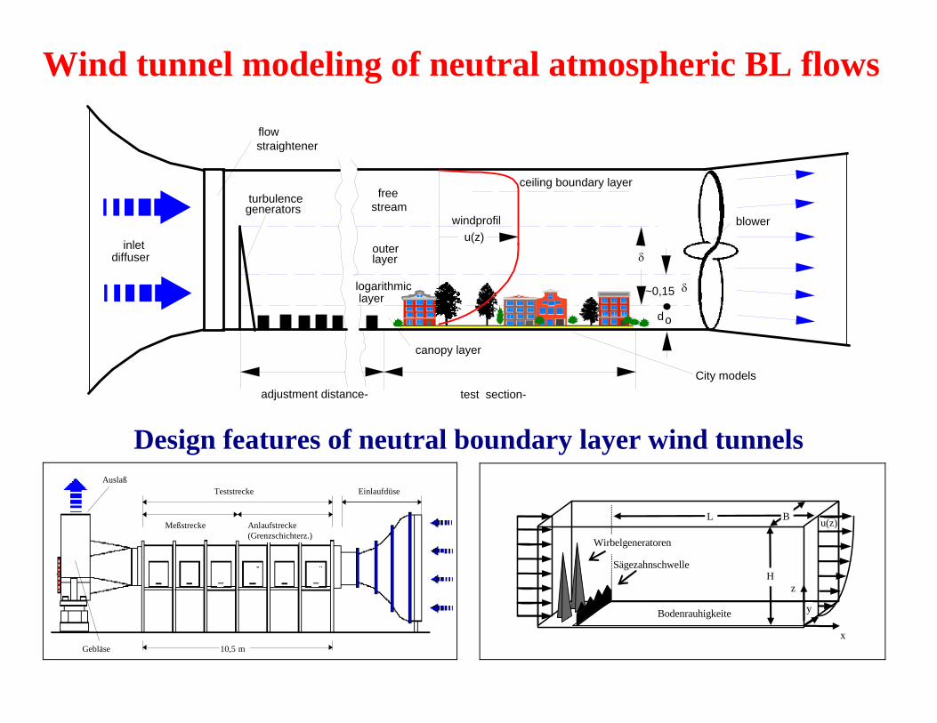
Wind tunnel modeling of neutral atmospheric BL flows

turbulencegenerators

flowstraightener

freestream

outerlayer

logarithmiclayer

bloweru(z)

ceiling boundary layer

adjustment distance- test section-City models

inletdiffuser

windprofil

δ

do

~0,15 δ

canopy layer

Design features of neutral boundary layer wind tunnels

AAuslaß

Teststrecke

Meßstrecke Anlaufstrecke(Grenzschichterz.)

Einlaufdüse

10,5 mGebläse

Bodenrauhigkeite

L B u(z)

Wirbelgeneratoren

x

H Sägezahnschwelle

z

y

Basic properties of a wall-bounded turbulent flow Consider turbulent flow that is parallel and horizontally homogeneous in x direction (an idealization of a wind tunnel flow far away from the inlet) with mean (in Reynolds sense) velocity in this direction u(z).

Prandtl concept of mixing distance/length l': particle that carries momentum between flow levels separated by distance l' instantly attributes momentum to surrounding air as it arrives to the destination level. First-order approximation: ( ') ( ) ( / ) 'u z l u z u z l+ = + ∂ ∂ ,

( ') ( ) ( / ) 'u z l u z u z l− = − ∂ ∂ , or, in terms of velocity fluctuations, ( ') ( ) '('( ') / )u z l uz z zu l l u= + − = ∂ ∂+ ,

'( ') ( ') ( ) '( / )u z l u z l u zu z l = − − = − ∂ ∂− . Prandtl also supposed: ' '( / )sign( ')w l u z u= − ∂ ∂ . Multiplying 'w with 'u and averaging, we come to ' 'u w 2 2( / )l u z= − ∂ ∂ ,

where l=1/ 2

2'l is the mixing length at level z, which may be interpreted as characteristic integral turbulence length scale for momentum exchange at level z.

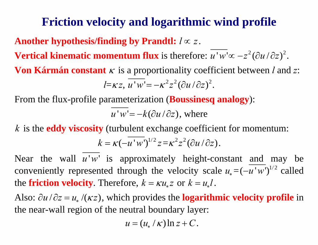
Friction velocity and logarithmic wind profile Another hypothesis/finding by Prandtl: l z∝ . Vertical kinematic momentum flux is therefore: ' 'u w 2 2( / )z u z∝ − ∂ ∂ . Von Kármán constant κ is a proportionality coefficient between l and z:

l=κ z, ' 'u w 2 2 2( / )z u zκ= − ∂ ∂ . From the flux-profile parameterization (Boussinesq analogy):

' 'u w ( / )k u z= − ∂ ∂ , where k is the eddy viscosity (turbulent exchange coefficient for momentum:

1/ 2( ' ')k u w zκ= − = 2 2 ( / )z u zκ ∂ ∂ . Near the wall ' 'u w is approximately height-constant and may be conveniently represented through the velocity scale u∗=

1/ 2( ' ')u w− called the friction velocity. Therefore, k u zκ ∗= or k u l∗= . Also: / /( )u z u zκ∗∂ ∂ = , which provides the logarithmic velocity profile in the near-wall region of the neutral boundary layer:

( / ) lnu u z Cκ∗= + .

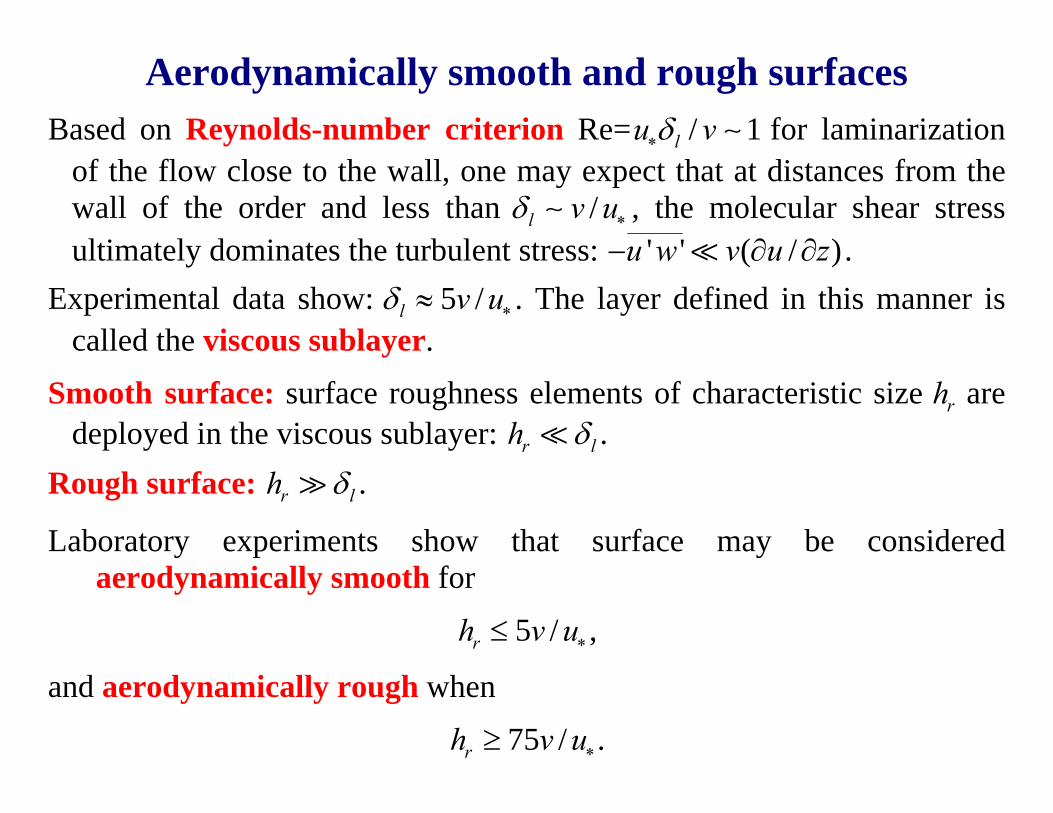
Aerodynamically smooth and rough surfaces Based on Reynolds-number criterion Re= / 1lu vδ∗ ∼ for laminarization

of the flow close to the wall, one may expect that at distances from the wall of the order and less than /l v uδ ∗∼ , the molecular shear stress ultimately dominates the turbulent stress: ' ' ( / )u w v u z− ∂ ∂ .

Experimental data show: 5 /l v uδ ∗≈ . The layer defined in this manner is called the viscous sublayer.

Smooth surface: surface roughness elements of characteristic size rh are deployed in the viscous sublayer: r lh δ .

Rough surface: r lh δ .

Laboratory experiments show that surface may be considered aerodynamically smooth for

5 /rh v u∗≤ ,

and aerodynamically rough when

75 /rh v u∗≥ .

Wind profile over smooth and rough surfaces Smooth-wall case: developed turbulent flow with ( / ) lnu u z Cκ∗= + is

realized at distances considerably larger than the length scale /l v uδ ∗∼ . Rough-wall case: flow is turbulent already in the immediate vicinity of

surface roughness elements, with mean flow velocity vanishing (u=0) at some level close to rh .

One may consider a reference level 0z close to the surface, where u=0,

0( / ) ln( / )u u z zκ∗= . Quantity 0z is called the aerodynamic surface roughness length or the surface roughness length for momentum.

Smooth-wall 0z is retrieved from / (1/ ) ln[ /( / )] su u z v u Cκ∗ ∗= + , where parameter 0(1/ ) ln[( / ) / ]sC v u zκ ∗= is about 5 (experiment):

0 / 0.1 /sCz e v u v uκ−∗ ∗= ≈ .

Rough-wall 0z is a function of the surface geometry, involving rh as one of parameters; generally speaking, 0z is growing with rh .

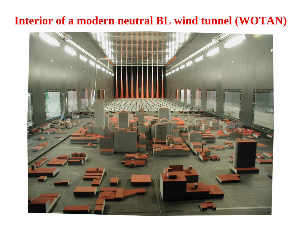
Interior of a modern neutral BL wind tunnel (WOTAN)

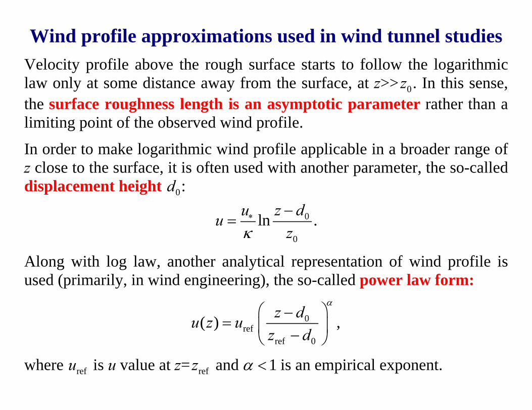
Wind profile approximations used in wind tunnel studies Velocity profile above the rough surface starts to follow the logarithmic law only at some distance away from the surface, at z>> 0z . In this sense, the surface roughness length is an asymptotic parameter rather than a limiting point of the observed wind profile.

In order to make logarithmic wind profile applicable in a broader range of z close to the surface, it is often used with another parameter, the so-called displacement height 0d :

0

0

ln z duuzκ

∗ −= .

Along with log law, another analytical representation of wind profile is used (primarily, in wind engineering), the so-called power law form:

0ref

ref 0

( ) ,z du z uz d

α⎛ ⎞−

= ⎜ ⎟−⎝ ⎠

where refu is u value at z= refz and 1α < is an empirical exponent.

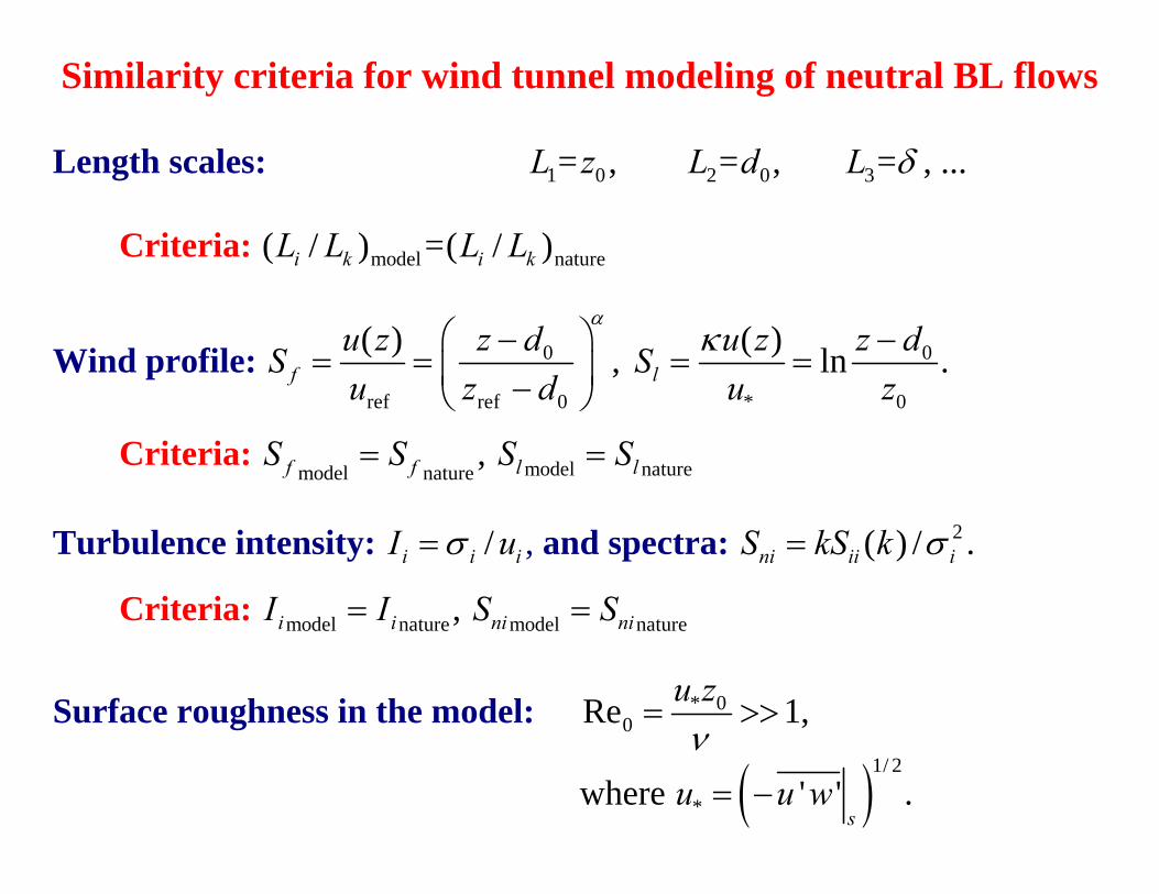
Similarity criteria for wind tunnel modeling of neutral BL flows

Length scales: 1L = 0z , 2L = 0d , 3L =δ , ...

Criteria: model( / )i kL L = nature( / )i kL L

Wind profile: 0

ref ref 0

( ) ,fu z z dSu z d

α⎛ ⎞−

= = ⎜ ⎟−⎝ ⎠ 0

* 0

( ) lnlu z z dSu z

κ −= = .

Criteria: model naturef fS S= , model naturel lS S=

Turbulence intensity: /i i iI uσ= , and spectra: 2( ) /ni ii iS kS k σ= .

Criteria: model naturei iI I= , model natureni niS S=

Surface roughness in the model: * 00Re 1u z

ν= >> ,

where ( )1/ 2

* ' 's

u u w= − .

Scaled mean wind profiles in WOTAN

Umean [m/s]0 2 4 6 8 10

10-1

100

101

102

z0 ≈ 0.20 ± 0.01 m

Umean [m/s]

Z FS[m

]

0 2 4 6 8 100

50

100

150

200

250

300

campaign IIcampaign I

power law exponentα ≈ 0.175 ± 0.05

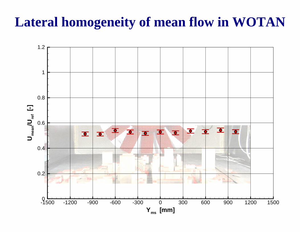
Lateral homogeneity of mean flow in WOTAN

Yms [mm]

Um

ean/U

ref

[-]

-1500 -1200 -900 -600 -300 0 300 600 900 1200 15000

0.2

0.4

0.6

0.8

1

1.2

Intensities of turbulent velocity fluctuations in WOTAN

IU [ - ]

Z FS[m

]

0 0.1 0.2 0.30

50

100

150

200

250

300measuredmod. roughrough

IV [ - ]

Z FS[m

]

0 0.1 0.2 0.30

50

100

150

200

250

300measuredmod. roughrough

IW [ - ]

Z FS[m

]0 0.1 0.2 0.3

0

50

100

150

200

250

300measuredmod. roughrough

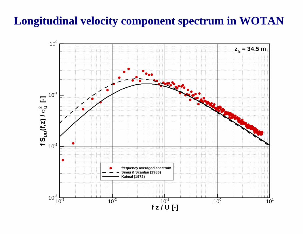
Longitudinal velocity component spectrum in WOTAN

f z / U [-]

fSU

U(f,

z)/σ

U2[-]

10-3 10-2 10-1 100 10110-3

10-2

10-1

100

frequency averaged spectrumSimiu & Scanlan (1986)Kaimal (1972)

zfs = 34.5 m

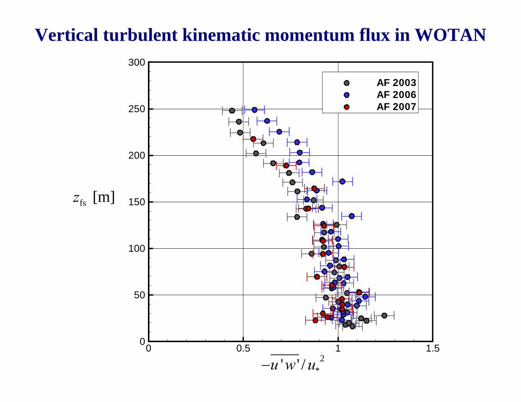
Vertical turbulent kinematic momentum flux in WOTAN

fs [m]z

0 0.5 1 1.50

50

100

150

200

250

300

AF 2003AF 2006AF 2007

2

*' ' /u w u−

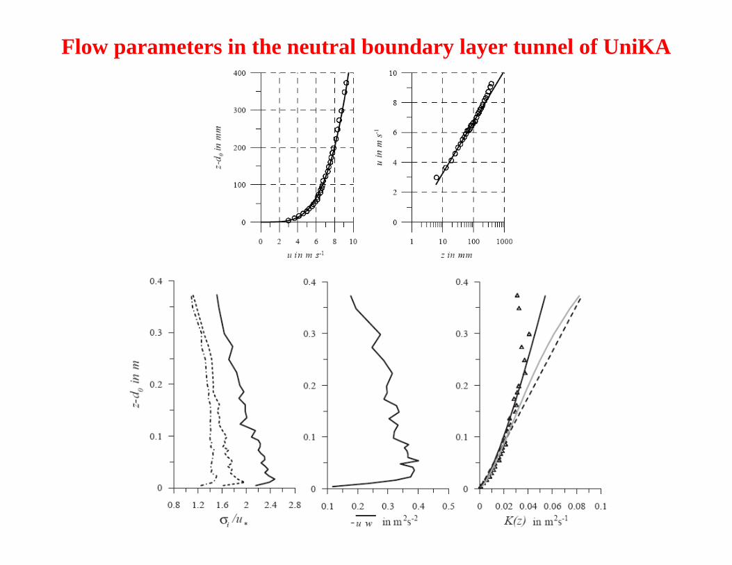
Flow parameters in the neutral boundary layer tunnel of UniKA

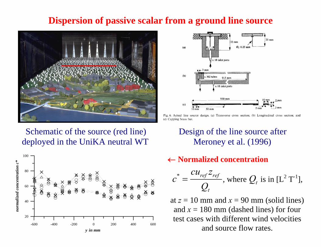
Dispersion of passive scalar from a ground line source

Schematic of the source (red line) Design of the line source after deployed in the UniKA neutral WT Meroney et al. (1996)

-600 -400 -200 0 200 400 600

y in mm

20

40

60

80

100

norm

aliz

ed c

once

ntra

tion

c* ← Normalized concentration

* ref ref

t

cu zc

Q= , where tQ is in [L2 T-1],

at z = 10 mm and x = 90 mm (solid lines) and x = 180 mm (dashed lines) for four test cases with different wind velocities

and source flow rates.

Longitudinal and vertical profiles of normalized concentration

0 200 400 600 800 1000

x in mm

0

20

40

60

80

100

norm

aliz

ed c

once

ntra

tion

c*

at z=10 mm

at x=45 mm0 50 100 150 200 250

normalized concentration c*

0

5

10

15

20

25

30

z in

mm

0 50 100

normalized concentration c*

0

10

20

30

40

50

60

70

80

z in

mm

at x=180 mm

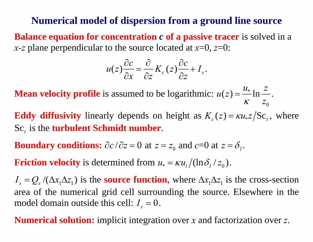
Numerical model of dispersion from a ground line source Balance equation for concentration c of a passive tracer is solved in a x-z plane perpendicular to the source located at x=0, z=0:

( ) ( )c sc cu z K z Ix z z∂ ∂ ∂

= +∂ ∂ ∂

.

Mean velocity profile is assumed to be logarithmic: *

0

( ) lnu zu zzκ

= .

Eddy diffusivity linearly depends on height as *( ) Scc tK z κu z= , where Sct is the turbulent Schmidt number.

Boundary conditions: / 0c z∂ ∂ = at 0z z= and c=0 at lz δ= .

Friction velocity is determined from * 0(ln / )l lu u zκ δ= .

1 1/( )s sI Q x z= Δ Δ is the source function, where 1 1x zΔ Δ is the cross-section area of the numerical grid cell surrounding the source. Elsewhere in the model domain outside this cell: 0sI = .

Numerical solution: implicit integration over x and factorization over z.

Model verification against the wind tunnel data Ground-level concentration (left plot)

10 100 1000x in m

0

10

20

30

40

c 0* (x)

0 200 400 600x in m

0

50

100

150

200

B(x

)

Wind tunnel data are gray symbols and lines. Dashed-dotted line shows numerical data for Sc 1t = . Other lines represent different analytical solutions considered in Kastner-Klein and Fedorovich (2002).

Concentration profiles at x = 45 m (left), x = 90 m (center), and x = 180 m (right)

0 4 8 12 16c*

0

0.2

0.4

0.6

0.8

z/z re

f

0 2 4 6 8c*

0

0.2

0.4

0.6

0.8

1

0 1 2 3 4c*

0

0.4

0.8

1.2

1.6

References Garratt, J. R., 1994: The Atmospheric Boundary Layer, Cambridge

University Press, 316pp. Kastner-Klein, P., and E. Fedorovich, 2002: Diffusion from a line source

deployed in a homogeneous roughness layer: interpretation of wind tunnel measurements by means of simple mathematical models. Atmospheric Environment, 36, 3709-3718.

Meroney, R. N., M. Pavageau, S. Rafailidis, and M. Schatzmann, 1996: Study of line source characteristics for 2-D physical modelling of pollutant dispersion in street canyons. Journal of Wind Engineering and Industrial Aerodynamics, 62, 37-65.

Sorbjan, Z., 1989: Structure of the Atmospheric Boundary Layer, Prentice Hall, 317 pp.

Thanks go to Petra Klein, Bernd Leitl, and Michael Schatzmann