Abbas El Gamal - Information Systems Laboratoryabbas/presentations/MSRI2006.pdf · Abbas El Gamal...
48
Capacity Theorems for Relay Channels Abbas El Gamal Department of Electrical Engineering Stanford University April, 2006 MSRI-06 1
Transcript of Abbas El Gamal - Information Systems Laboratoryabbas/presentations/MSRI2006.pdf · Abbas El Gamal...
Capacity Theorems for Relay Channels
Abbas El Gamal
Department of Electrical Engineering
Stanford University
April, 2006
MSRI-06 1

Relay Channel
• Discrete-memoryless relay channel [vM’71]
W Xn
Xn1
p(y, y1|x, x1)
Relay Encoder
Y n
Y n1
Encoder Decoder W
• Goal: Reliably communicate message W ∈ [1, 2nR] from X to Y with the
help of relay node (X1, Y1)
• Relay transmission:
◦ Classical: x1i = fi(y11, y12, . . . , y1(i−1))
◦ Without-delay: x1i = fi(y11, y12, . . . , y1i)
MSRI-06 2
Capacity
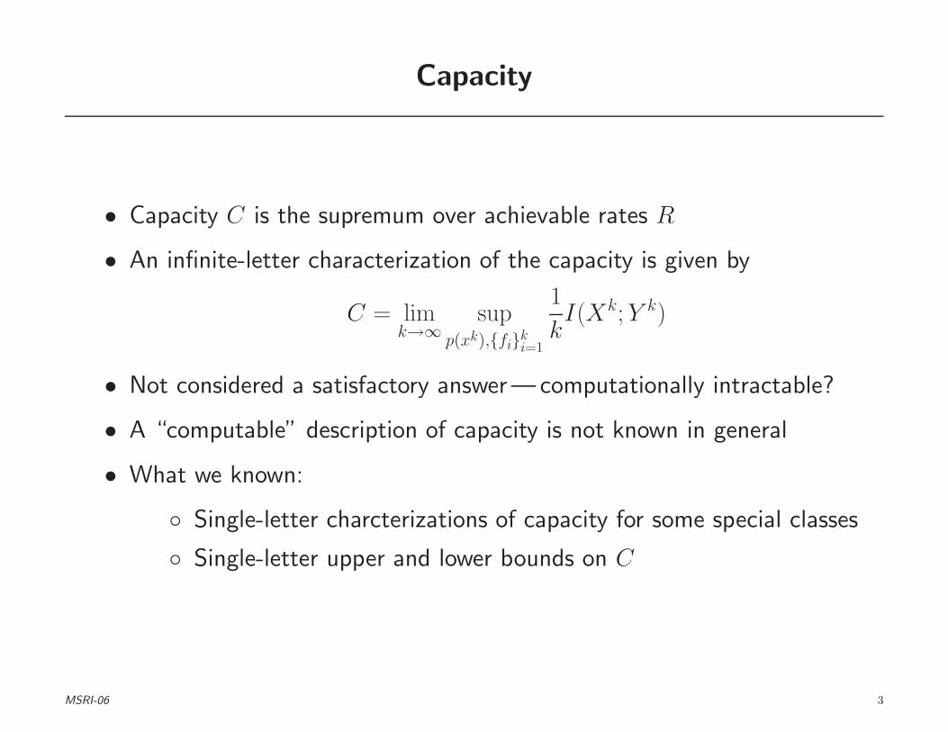
• Capacity C is the supremum over achievable rates R
• An infinite-letter characterization of the capacity is given by
C = limk→∞
supp(xk),{fi}k
i=1
1
kI(Xk; Y k)
• Not considered a satisfactory answer— computationally intractable?
• A “computable” description of capacity is not known in general
• What we known:
◦ Single-letter charcterizations of capacity for some special classes
◦ Single-letter upper and lower bounds on C
MSRI-06 3

My Encounter with The Relay Channel
• Visited University of Hawaii in Spring 1976
◦ ARPA Aloha packet radio project
• David Slepian introduced me to the problem
◦ Send data directly and via a satellite
• Worked on it as part of my PhD thesis and with my first student M. Aref
• Little interest from information theory and communication community
for years
• Renewed interest motivated by wireless networks — work with S. Zahedi,
M. Mohseni, N. Hassanpour, and J. Mammen
MSRI-06 4
Early Work 1997–1980
[CE’79 ] Cover, El Gamal, “Capacity theorems for the relay channel,” IT, 1979
◦ Cutset upper bound on C
◦ Block Markov coding (decode-and-forward)
◦ Capacity of degraded relay channels
◦ Capacity of relay channel with feedback
◦ Side-information coding (compress-and-forward)
◦ General lower bound on C—combining partial decode-and-forward
and compress and forward
[EA’82 ] El Gamal, Aref, “The Capacity of the semi-determininstic relay
channel,”IT Trans., 1982 (partial decode-and-forward)
• El Gamal, “On information flow in relay networks,”IEEE NTC, 1980
(cutset bound for relay networks)
• Aref, “Information flow in relay networks,” PhD Thesis, Stanford 1980
(capacity of degraded relay networks)
MSRI-06 5

Recent Work 2002–Present
[EZ’05 ] El Gamal, Zahedi, “Capacity of a class of of relay channels with
orthogonal components,” IT Trans., 2005 (partial decode-and-forward)
[EMZ’06 ] El Gamal, Mohseni, Zahedi, “Bounds on Capacity and Minimum
Energy-Per-Bit for AWGN Relay Channels,” to appear in IT Trans.
◦ Compress-and-forward with time sharing
◦ Capacity of FD-AWGN relay channels with linear relaying functions
◦ Bounds on minimum energy-per-bit that differ by factor < 1.7
[EH’05 ] El Gamal, Hassanpour, “Relay-without-delay,” ISIT, 2005
El Gamal, Hassanpour, “Capacity Theorems for the relay-without-delay
channel,” Allerton, 2005
[EM’06 ] El Gamal, Mammen, “Relay networks with delays,” UCSD, 2006
MSRI-06 6
Outline
• Classical relay:
◦ Cutset upper bound
◦ Partial decode-and-forward
◦ Compress-and-forward
◦ Upper and lower bounds on capacity of AWGN relay channel
• Relay-without-delay:
◦ New cutset bound
◦ Instantaneous relaying
◦ Lower bound and capacity results (see poster by N. Hassanpour)
MSRI-06 7
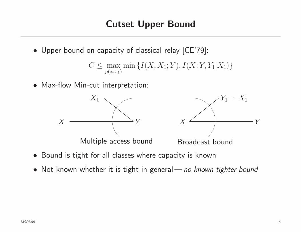
Cutset Upper Bound
• Upper bound on capacity of classical relay [CE’79]:
C ≤ maxp(x,x1)
min {I(X, X1; Y ), I(X ; Y, Y1|X1)}
• Max-flow Min-cut interpretation:
XX
X1
YY
Y1 : X1
Multiple access bound Broadcast bound
• Bound is tight for all classes where capacity is known
• Not known whether it is tight in general— no known tighter bound
MSRI-06 8

Partial Decode-and-Forward
• Lower bound [CE’79]:
C ≥ maxp(u,x,x1)
min {I(X, X1; Y ), I(X ; Y |X1, U ) + I(U ; Y1|X1)}
• Transmission in B blocks. In block b:W1 W2 W3 WB−1 WB
1 2 3 B − 1 B. . .
. . .
◦ The relay and sender “coherently” send information (X1) to Y
◦ The sender also superposes a new message Wb (thr’ X)
◦ The relay decodes part of Wb (represented by U)
◦ The receiver decodes X1, which helps it decode Wb−1 (U then X)
• Bound is tight for all cases where capacity is known:
◦ Degraded: (X → (Y1, X1) → Y ). Set U = X [CE’79]
◦ Semideterministic: (Y1 = g(X, X1)). Set U = Y1 [EA’82]
◦ Relay channel with orthogonal components (X = (XD, XR),
p(y|xD, x1)p(y1|xR, x1)). Set U = XR [EZ’05]
MSRI-06 9

Compress-and-Forward
• The relay can help even without decoding any part of the message
• Compress-and-forward scheme [CE’79]:
◦ Again transmission in B blocks
◦ Relay “quantizes” the received sequence in previous block andsends it to the receiver (a la Wyner-Ziv)
W WX
Y1 : X1
Y
Y1
◦ Relay and the sender do not cooperate (interfere with each other)
C ≥ maxp(x)p(x1)p(y1|y1,x1)
min{I(X ; Y, Y1|X1), I(X,X1; Y ) − I(Y1; Y1|X,X1)}
• Except for some asymptotic results, not optimal for any known class
• Partial decode-and-forward and compress-and-forward can be combined
(Theorem 7 of [CE’79])
MSRI-06 10

Compress-and-Forward with Time-Sharing [EMZ’06]
• Compress-and-forward achievable rate is not convex
• Can be improved by time-sharing, which gives the bound
C ≥ max min{I(X ; Y, Y1|X1, Q), I(X, X1; Y |Q) − I(Y1; Y1|X,X1, Q)},where the maximization is over p(q)p(x|q)p(x1|q)p(y1|y1, x1, q)
• Example: FD-AWGN relay channel [EMZ’06]
MSRI-06 11
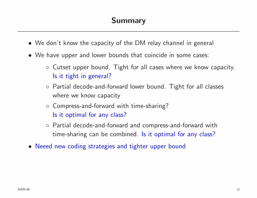
Summary
• We don’t know the capacity of the DM relay channel in general
• We have upper and lower bounds that coincide in some cases:
◦ Cutset upper bound. Tight for all cases where we know capacity.
Is it tight in general?
◦ Partial decode-and-forward lower bound. Tight for all classes
where we know capacity
◦ Compress-and-forward with time-sharing?
Is it optimal for any class?
◦ Partial decode-and-forward and compress-and-forward with
time-sharing can be combined. Is it optimal for any class?
• Neeed new coding strategies and tighter upper bound
MSRI-06 12
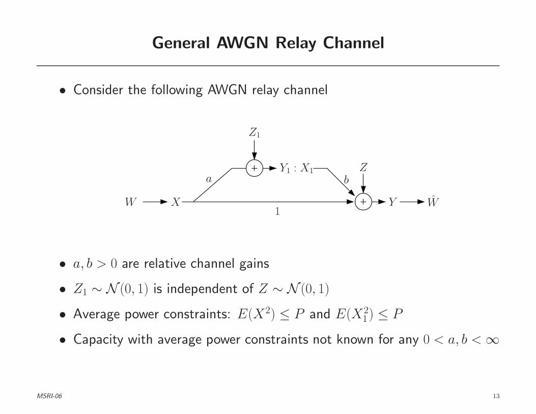
General AWGN Relay Channel
• Consider the following AWGN relay channel
XW W
a
Z1
Y1 : X1
bZ
Y1
• a, b > 0 are relative channel gains
• Z1 ∼ N (0, 1) is independent of Z ∼ N (0, 1)
• Average power constraints: E(X2) ≤ P and E(X21) ≤ P
• Capacity with average power constraints not known for any 0 < a, b < ∞
MSRI-06 13
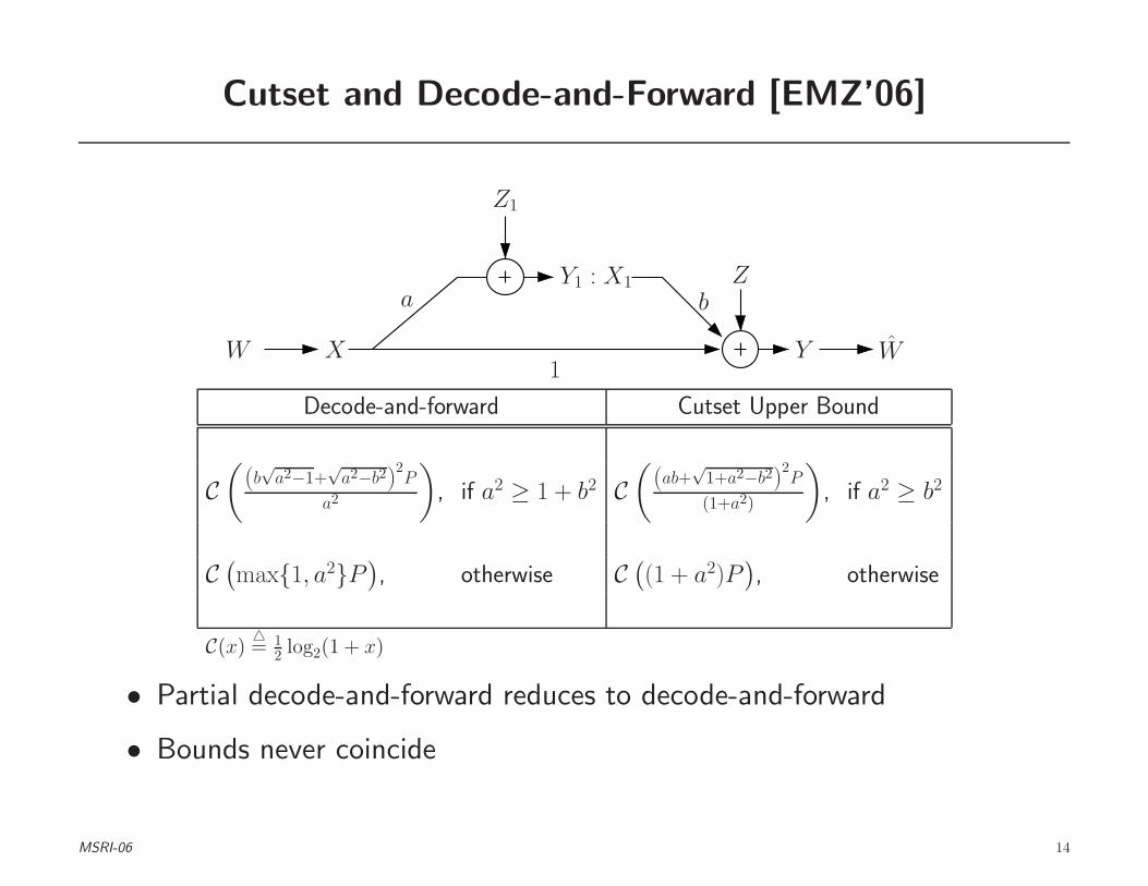
Cutset and Decode-and-Forward [EMZ’06]
XW W
a
Z1
Y1 : X1
bZ
Y1
Decode-and-forward Cutset Upper Bound
C(
(b√
a2−1+√
a2−b2)2P
a2
)
, if a2 ≥ 1 + b2 C(
(ab+√
1+a2−b2)2P
(1+a2)
)
, if a2 ≥ b2
C(
max{1, a2}P)
, otherwise C(
(1 + a2)P)
, otherwise
C(x)△= 1
2 log2(1 + x)
• Partial decode-and-forward reduces to decode-and-forward
• Bounds never coincide
MSRI-06 14
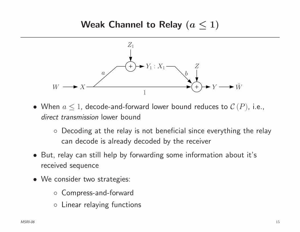
Weak Channel to Relay (a ≤ 1)
XW W
a
Z1
Y1 : X1
bZ
Y1
• When a ≤ 1, decode-and-forward lower bound reduces to C (P ), i.e.,
direct transmission lower bound
◦ Decoding at the relay is not beneficial since everything the relay
can decode is already decoded by the receiver
• But, relay can still help by forwarding some information about it’s
received sequence
• We consider two strategies:
◦ Compress-and-forward
◦ Linear relaying functions
MSRI-06 15

Compress-and-Forward [EMZ’06]
• Achievable rate using compress-and-forward
R = maxp(x)p(x1)p(y1|y1,x1)
min{I(X,X1; Y ) − I(Y1; Y1|X,X1), I(X ; Y, Y1|X1)},
• The optimal choice of p(x)p(x1)p(y1|y1, x1) is not known
• Assume X, X1 and Y1 Gaussian:
X
a
Y
α
Z ′Z1
Y1 : X1
bZ
Y1
C ≥ C(
P
(
1 +a2b2P
P (1 + a2 + b2) + 1
))
• As b → ∞, this bound becomes tight (coincides with broadcast bound)
MSRI-06 16

Comparison of Bounds
• a = 1 and b = 2
0 1 2 3 4 5 6 7 8 9 100
0.5
1
1.5
2
2.5
SNR
Upper Bound
Compress-forward
Decode-forward
Rat
e(B
its/
Tra
ns.)
MSRI-06 17

Frequency-Division AWGN Relay Channel [EMZ’06]
• Model motivated by wireless communication:
X
a
Z1
Y1 : X1b
ZS
ZR
YS
YR
1
• Bounds on capacity of FD-AWGN relay
Decode-and-forward Cutset Upper Bound
C(
P(
1 + b2 + b2P))
, if a2 ≥ 1 + b2 + b2P C(
P(
1 + b2 + b2P))
, if a2 ≥ b2 + b2P
C(
max{1, a2}P)
, otherwise C(
(1 + a2)P)
, otherwise
• If a2 ≥ 1 + b2 + b2P capacity is C(
P(
1 + b2 + b2P))
(decode-forward)
• Model same as without delay
MSRI-06 18

FD-AWGN – Weak Channel to Relay (a ≤ 1) [EMZ’06]
• Again if a ≤ 1, decode-and-forward reduces to direct transmission
X
a
Z1
Y1 : X1b
ZS
ZR
YS
YR
1
• Can improve rate using compress-and-forward. Using Gaussian signals,
we obtain:
C ≥ C(
P
(
1 +a2b2P (1 + P )
a2P + (1 + P )(1 + b2P )
))
• As b or P → ∞, compress-and-forward becomes optimal
MSRI-06 19

FD-AWGN – Compress-and-Forward With Time-Sharing
• For small P , compress-and-forward is ineffective due to low SNR of Y1
0 P
Rate with time-sharingRate
• Rate can be improved by time-sharing at the broadcast side (X sends at
power P/α for fraction 0 < α ≤ 1 and 0, otherwise) to:
C ≥ max0<α≤1
αC
P
α
1 +
a2
1 +(
1 + a2PP+α
)/(
−1 + (1 + b2P )1α
)
MSRI-06 20

Comparison of Bounds for FD AWGN
• Example: a = 1 and b = 2
0 1 2 3 4 5 6 7 8 9 100
0.5
1
1.5
2
2.5
SNR
Upper Bound
Compress-forward
Decode-forwardRat
e(B
its/
Tra
ns.)
MSRI-06 21

Linear Relaying
• Assume relay can only transmit a linear combination of the past received
symbols, i.e., x1(i+1) =∑i
j=1 dijy1j
• Using vector notation
X1 = DY1,
where D = [dij]k×k is a strictly lower triangular matrix and
X1 = (X11, X12, . . . , X1k)T and Y1 = (Y11, Y12, . . . , Y1k)
T
XnW W
a
Zn1
Y n1 Xn
1D
bZn
Y n1
• Let C(l) be the capacity with linear relaying subject to the power
constraints
MSRI-06 22

Capacity with Linear Relaying
• Capacity with linear relaying can be expressed as
C(l) = supk
1
kC
(l)k = lim
k→∞1
kC
(l)k
where
C(l)k = sup
PXk ,D
I(Xk; Y k)
subject to
◦ Sender power constraint:∑k
i=1 E(X2i ) ≤ kP
◦ Relay power constraint:∑k
i=1 E(x21i) ≤ kP
◦ Causality constraint: D strictly lower triangular
MSRI-06 23
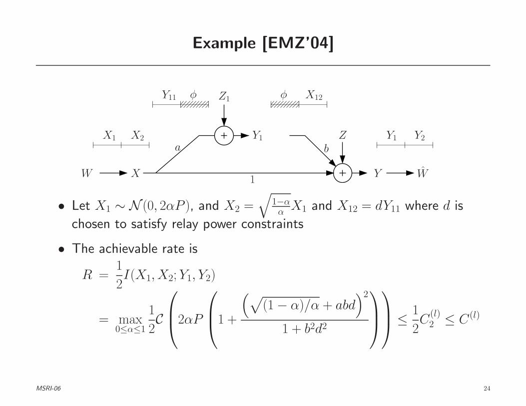
Example [EMZ’04]
W X
Y1
Y
a b
1
Z
Z1
W
X1 X2
X12
Y1 Y2
φφY11
• Let X1 ∼ N (0, 2αP ), and X2 =√
1−αα
X1 and X12 = dY11 where d is
chosen to satisfy relay power constraints
• The achievable rate is
R =1
2I(X1, X2; Y1, Y2)
= max0≤α≤1
1
2C
2αP
1 +
(
√
(1 − α)/α + abd)2
1 + b2d2
≤ 1
2C
(l)2 ≤ C(l)
MSRI-06 24
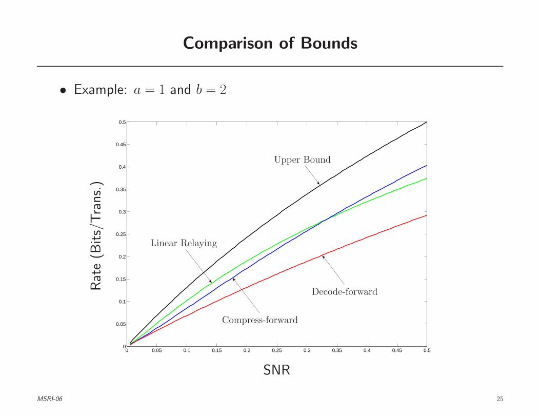
Comparison of Bounds
• Example: a = 1 and b = 2
0 0.05 0.1 0.15 0.2 0.25 0.3 0.35 0.4 0.45 0.50
0.05
0.1
0.15
0.2
0.25
0.3
0.35
0.4
0.45
0.5
SNR
Upper Bound
Linear Relaying
Compress-forward
Decode-forwardRat
e(B
its/
Tra
ns.)
MSRI-06 25

Capacity with Linear Relaying for General AWGN
• Gaussian distribution PXk maximizes C(l)k = supP
Xk ,D I(Xk; Y k)
• Problem reduces to:
Maximize limk→∞
1
2klog
|(I + abD)Σx(I + abD)T + (I + b2DDT )||(I + b2DDT )|
Subject to Σx � 0
tr(Σx) ≤ kP
tr(a2ΣxDTD + DTD) ≤ kP
dij = 0 for j ≥ i
• Σx = E(XXT ) and D are variables of the problem
• Sequence of non-convex problems (open problem)
• “Single-letter” characterization can be found for FD-AWGN relay channel
MSRI-06 26

FD-AWGN Relay Channel with Linear Relaying
• Example: Consider the following “amplify-and-forward” scheme
X
a
Z1
Y1b
ZS
ZR
YS
YR
1
X
Y1
X1
YR
YS
• X ∼ N (0, P ) and X1 = dY1 where d is chosen to satisfy the relay power
constraint
• The achievable rate for this scheme is given by I(X ; YS, YR)
C(l)1 = C
(
P
(
1 +a2b2P
1 + (a2 + b2)P
))
MSRI-06 27
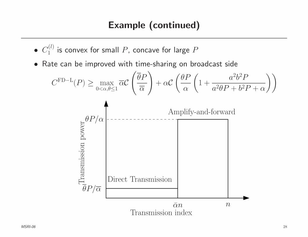
Example (continued)
• C(l)1 is convex for small P , concave for large P
• Rate can be improved with time-sharing on broadcast side
CFD−L(P ) ≥ max0<α,θ≤1
αC(
θP
α
)
+ αC(
θP
α
(
1 +a2b2P
a2θP + b2P + α
))
Amplify-and-forward
Direct Transmission
Transmission index
Tra
nsm
issi
onpow
er
θP/α
αn n
θP/α
MSRI-06 28

Capacity of FD-AWGN Relay Channel with Linear Relaying
• Capacity with linear relaying for the FD-AWGN model can be expressed
as
C(l) = supk
1
kC
(l)k = lim
k→∞1
kC
(l)k ,
where
C(l)k = sup
PXk ,D
I(Xk; Y kS , Y k
R)
Subject to:
◦ Sender power constraint:∑k
i=1 E(X2i ) ≤ kP
◦ Relay power constraint:∑k
i=1 E(X21i) ≤ kP
◦ Causality constraint: D lower triangular
MSRI-06 29
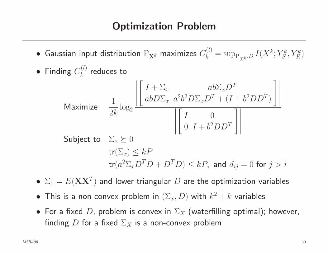
Optimization Problem
• Gaussian input distribution PXk maximizes C(l)k = supP
Xk ,D I(Xk; Y kS , Y k
R)
• Finding C(l)k reduces to
Maximize1
2klog2
∣
∣
∣
∣
∣
[
I + Σx abΣxDT
abDΣx a2b2DΣxDT + (I + b2DDT )
]∣
∣
∣
∣
∣
∣
∣
∣
∣
∣
[
I 0
0 I + b2DDT
]∣
∣
∣
∣
∣
Subject to Σx � 0
tr(Σx) ≤ kP
tr(a2ΣxDTD + DTD) ≤ kP, and dij = 0 for j > i
• Σx = E(XXT ) and lower triangular D are the optimization variables
• This is a non-convex problem in (Σx, D) with k2 + k variables
• For a fixed D, problem is convex in ΣX (waterfilling optimal); however,
finding D for a fixed ΣX is a non-convex problem
MSRI-06 30
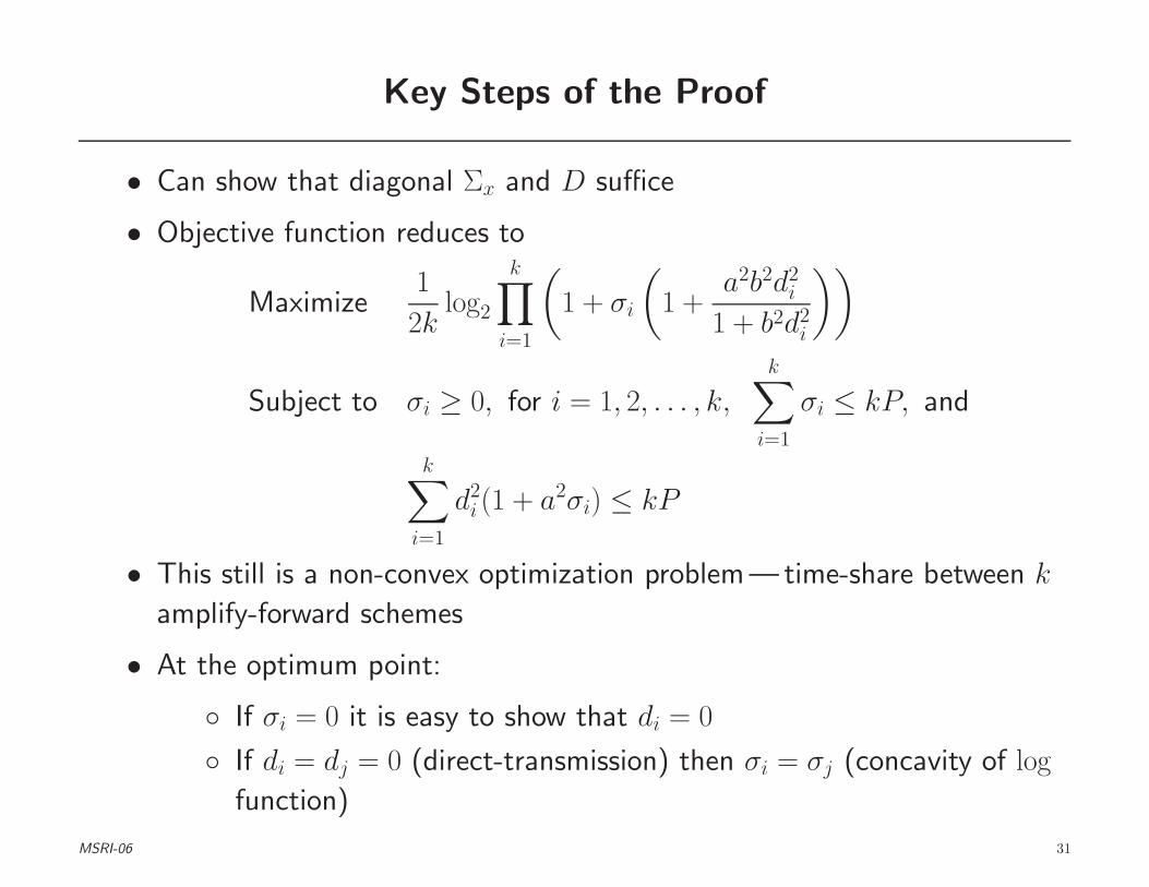
Key Steps of the Proof
• Can show that diagonal Σx and D suffice
• Objective function reduces to
Maximize1
2klog2
k∏
i=1
(
1 + σi
(
1 +a2b2d2
i
1 + b2d2i
))
Subject to σi ≥ 0, for i = 1, 2, . . . , k,
k∑
i=1
σi ≤ kP, and
k∑
i=1
d2i (1 + a2σi) ≤ kP
• This still is a non-convex optimization problem— time-share between k
amplify-forward schemes
• At the optimum point:
◦ If σi = 0 it is easy to show that di = 0
◦ If di = dj = 0 (direct-transmission) then σi = σj (concavity of log
function)
MSRI-06 31
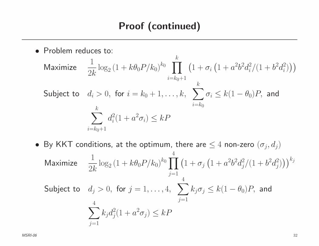
Proof (continued)
• Problem reduces to:
Maximize1
2klog2 (1 + kθ0P/k0)
k0
k∏
i=k0+1
(
1 + σi
(
1 + a2b2d2i/(1 + b2d2
i )))
Subject to di > 0, for i = k0 + 1, . . . , k,k∑
i=k0
σi ≤ k(1 − θ0)P, and
k∑
i=k0+1
d2i (1 + a2σi) ≤ kP
• By KKT conditions, at the optimum, there are ≤ 4 non-zero (σj, dj)
Maximize1
2klog2 (1 + kθ0P/k0)
k0
4∏
j=1
(
1 + σj
(
1 + a2b2d2j/(1 + b2d2
j)))kj
Subject to dj > 0, for j = 1, . . . , 4,4∑
j=1
kjσj ≤ k(1 − θ0)P, and
4∑
j=1
kjd2j(1 + a2σj) ≤ kP
MSRI-06 32

Capacity of FD-AWGN Relay with Linear Relaying [EMZ’06]
• Taking the limit as k → ∞, we obtain
C(l) = max α0C(
θ0P
α0
)
+
4∑
j=1
αjC(
θjP
αj
(
1 +a2b2ηj
1 + b2ηj
))
,
subject to αj, θj ≥ 0, ηj > 0,∑4
j=0 αj =∑4
j=0 θj = 1, and∑4
j=1 ηj
(
a2θjP + αj
)
= P
• Time-share between direct transmission and 4 amplify-forward regimes
• A non-convex optimization problem, but with only 14 variables and 3
constraints
• We haven’t been able to find any example where optimal requires > 2
amplify-forward regimes (in addition to direct transmission)
MSRI-06 33
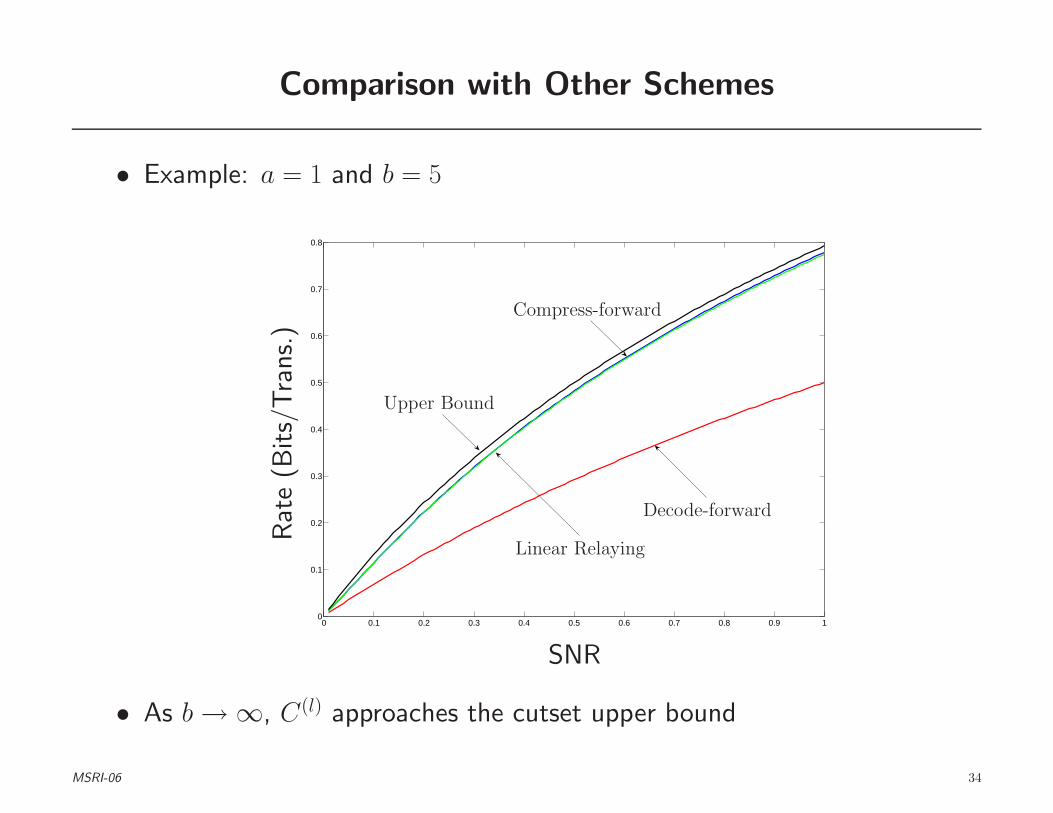
Comparison with Other Schemes
• Example: a = 1 and b = 5
0 0.1 0.2 0.3 0.4 0.5 0.6 0.7 0.8 0.9 10
0.1
0.2
0.3
0.4
0.5
0.6
0.7
0.8
SNR
Upper Bound
Compress-forward
Decode-forward
Linear Relaying
Rat
e(B
its/
Tra
ns.)
• As b → ∞, C(l) approaches the cutset upper bound
MSRI-06 34

Summary
• For general AWGN relay channel:
◦ Bounds are never tight for any 0 < a, b < ∞◦ Compress-and-forward becomes optimal as b → ∞◦ Linear relaying can beat compress-and-forward—we don’t have a
computable expression for capacity with linear relaying
• For FD-AWGN relay channel:
◦ Decode-and-forward is optimal (bound coincides with cutset)
when a2 ≥ 1 + b2 + b2P
◦ Compress-and-forward becomes optimal as b or P → ∞.
Time-sharing improves rate for small P
◦ We have a computable form of capacity with linear
relaying — time-sharing between direct transmission and at most 4
amplify-and-forward regimes
MSRI-06 35

Relay-Without-Delay (RWD)
• Suppose the delay from the sender X to the receiver Y is longer than to
the relay (X1, Y1), so that x1i can depend on its current, in addition to
past received symbols, i.e.,
x1i = fi(y11, y12, . . . , y1(i−1), y1i)
• Relay-without-delay:
W Xn
Xn1
p(y1|x)p(y|x, x1, y1)
Relay Encoder
Y n
Y n1
W
• Again, wish to reliably communicate W ∈ [1, 2nR] from X to Y
MSRI-06 36
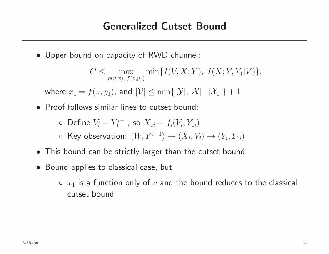
Generalized Cutset Bound
• Upper bound on capacity of RWD channel:
C ≤ maxp(v,x), f(v,y1)
min{I(V, X ; Y ), I(X ; Y, Y1|V )},
where x1 = f(v, y1), and |V| ≤ min{|Y|, |X | · |X1|} + 1
• Proof follows similar lines to cutset bound:
◦ Define Vi = Y i−11 , so X1i = fi(Vi, Y1i)
◦ Key observation: (W, Y i−1) → (Xi, Vi) → (Yi, Y1i)
• This bound can be strictly larger than the cutset bound
• Bound applies to classical case, but
◦ x1 is a function only of v and the bound reduces to the classical
cutset bound
MSRI-06 37
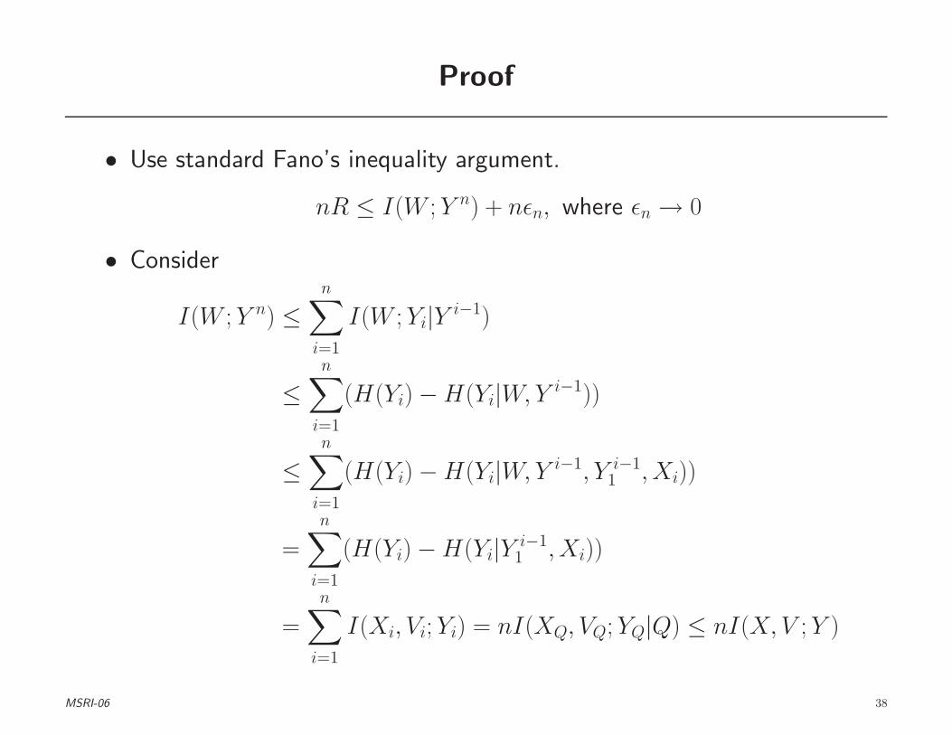
Proof
• Use standard Fano’s inequality argument.
nR ≤ I(W ; Y n) + nǫn, where ǫn → 0
• Consider
I(W ; Y n) ≤n∑
i=1
I(W ; Yi|Y i−1)
≤n∑
i=1
(H(Yi) − H(Yi|W, Y i−1))
≤n∑
i=1
(H(Yi) − H(Yi|W, Y i−1, Y i−11 , Xi))
=n∑
i=1
(H(Yi) − H(Yi|Y i−11 , Xi))
=n∑
i=1
I(Xi, Vi; Yi) = nI(XQ, VQ; YQ|Q) ≤ nI(X,V ; Y )
MSRI-06 38

• Next consider
I(W ; Y n) ≤ I(W ; Y n, Y n1 )
=n∑
i=1
I(W ; Yi, Y1i|Y i−1, Y i−11 )
=n∑
i=1
H(Yi, Y1i|Y i−1, Y i−11 ) − H(Yi, Y1i|Y i−1, Y i−1
1 , W )
≤n∑
i=1
H(Yi, Y1i|Vi) − H(Yi, Y1i|Y i−1, Y i−11 , W, Xi)
≤n∑
i=1
H(Yi, Y1i|Vi) − H(Yi, Y1i|Vi, Xi)
=
n∑
i=1
I(Xi; Yi, Y1i|Vi) = nI(X ; Y, Y1|V )
MSRI-06 39
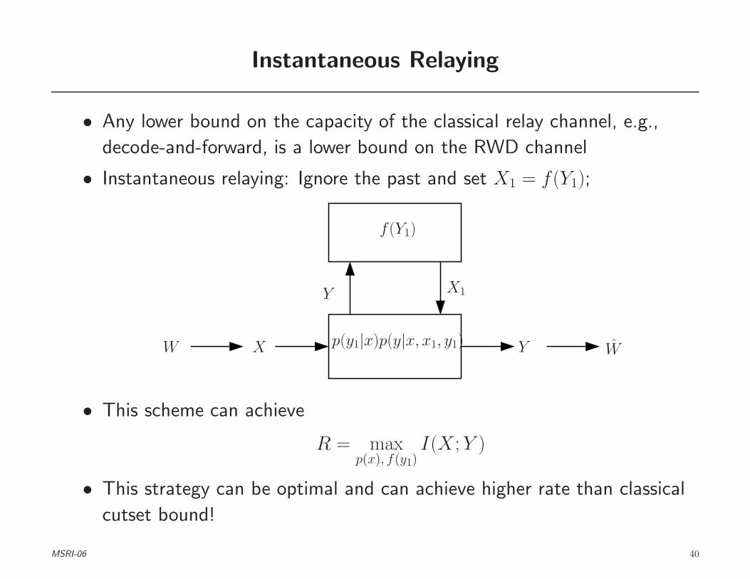
Instantaneous Relaying
• Any lower bound on the capacity of the classical relay channel, e.g.,
decode-and-forward, is a lower bound on the RWD channel
• Instantaneous relaying: Ignore the past and set X1 = f(Y1);
W X
X1
p(y1|x)p(y|x, x1, y1)
f(Y1)
Y
Y
W
• This scheme can achieve
R = maxp(x), f(y1)
I(X ; Y )
• This strategy can be optimal and can achieve higher rate than classical
cutset bound!
MSRI-06 40

Sato Example
• Consider the following DW relay channel [Sato’76]. Y1 = X and
XX YY00
1
1
22
0.5
0.5
0.5
0.5
00
1
1
22
X1 = 0 X1 = 1
• The capacity of the classical case is 1.161878 bits/transmission [CE’79]
◦ Coincides with cutset bound
• The upper bound on the capacity without delay gives:
C ≤ 2(log 3 − 1) = 1.169925 bits/transmission
• Instantaneous relaying with input distribution(
39,
29,
49
)
and the mapping
from X to X1 of 0 → 0, 1 → 1, 2 → 1 achieves this bound!!
• Capacity of this RWD channel > classical, which is = cutset bound
MSRI-06 41
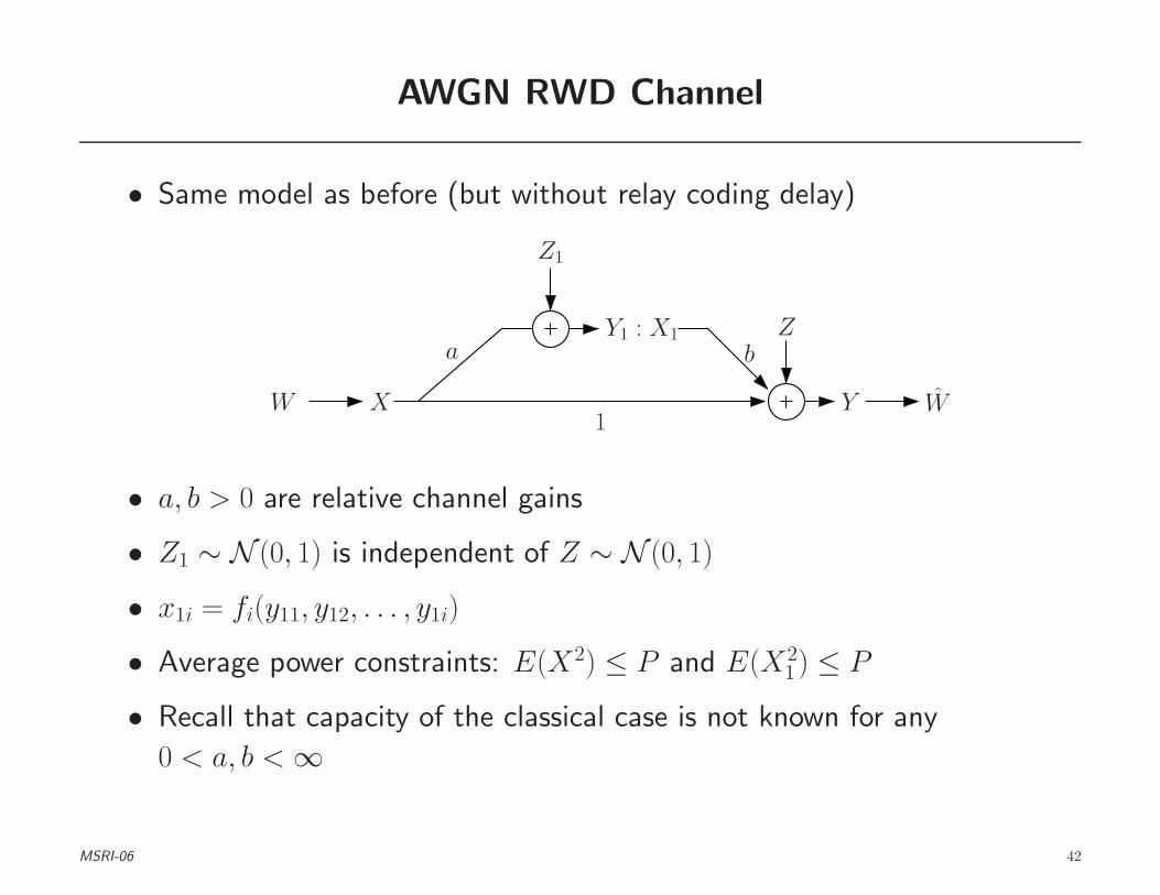
AWGN RWD Channel
• Same model as before (but without relay coding delay)
XW W
a
Z1
Y1 : X1
bZ
Y1
• a, b > 0 are relative channel gains
• Z1 ∼ N (0, 1) is independent of Z ∼ N (0, 1)
• x1i = fi(y11, y12, . . . , y1i)
• Average power constraints: E(X2) ≤ P and E(X21) ≤ P
• Recall that capacity of the classical case is not known for any
0 < a, b < ∞
MSRI-06 42
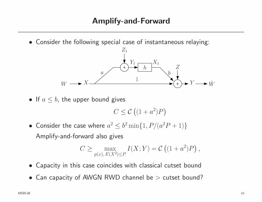
Amplify-and-Forward
• Consider the following special case of instantaneous relaying:
XW W
a
Z1
Y1 X1h
bZ
Y1
• If a ≤ b, the upper bound gives
C ≤ C(
(1 + a2)P)
• Consider the case where a2 ≤ b2 min{1, P/(a2P + 1)}Amplify-and-forward also gives
C ≥ maxp(x), E(X2)≤P
I(X ; Y ) = C(
(1 + a2)P)
,
• Capacity in this case coincides with classical cutset bound
• Can capacity of AWGN RWD channel be > cutset bound?
MSRI-06 43
New Lower Bound on Capacity of RWD Channel
• Idea: Use a superposition of partial decode-and-forward and
instantaneous relaying
• Achieves the lower bound:
C ≥ maxp(u,v,x), f(v,y1)
min{I(V, X ; Y ), I(U ; Y1|V ) + I(X ; Y |V, U )}
◦ U represents the information decoded by the relay in partial
decode-and-forward and V (replacing X1) represents the
information sent coherently by the sender and the relay to help the
receiver decode the previous U
◦ Each xn1 codeword in partial decode-and-forward is replaced by a
vn codeword, and at time i the relay sends x1i = f(vi, y1i)
• This bound coincides with the generalized cutset bound for degraded
and semi-deterministic RWD channels
• Same superposition idea can be used to obain new compress-and-forward
lower bound
MSRI-06 44
Achievable Rate for AWGN RWD Channel
• Restrict previous scheme to superposition of decode-and-forward and
amplify-and-forward:
◦ Let U = X = V + X ′, where V ∼ N (0, αP ) and X ′ ∼ N (0, αP )
are independent, for 0 ≤ α ≤ 1 and α = 1 − α
◦ Let X1 be a normalized convex combination of Y1 and V
X1 = h(βY1 + βV ), 0 ≤ β ≤ 1
• Using the power constraint on the relay sender, we obtain
h2 =P
(β + aβ)2αP + β2(a2αP + N)
• Substituting the above choice of (U, V, X,X1), we obtain
CRWD−AWGN ≥ maxα, β
min
{
C(
a2αP)
, C(
αP (bh(aβ + β) + 1)2 + αP (bhaβ + 1)2
(1 + (βbh)2)
)}
MSRI-06 45
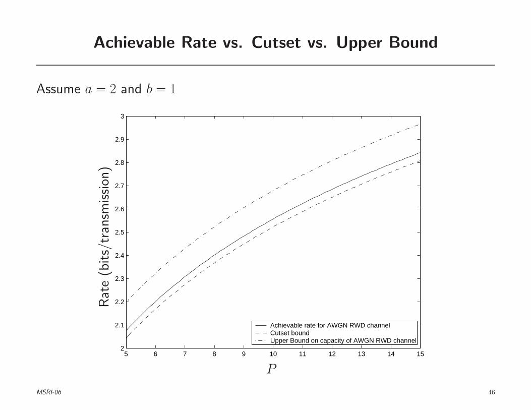
Achievable Rate vs. Cutset vs. Upper Bound
Assume a = 2 and b = 1
5 6 7 8 9 10 11 12 13 14 152
2.1
2.2
2.3
2.4
2.5
2.6
2.7
2.8
2.9
3
Achievable rate for AWGN RWD channelCutset boundUpper Bound on capacity of AWGN RWD channel
P
Rat
e(b
its/
tran
smission
)
MSRI-06 46

Classical vs. RWD Relay Channels
Result Classical Relay RWD
Capacity Not known in general Not known in general
Can be > classical
Upper bound maxp(x,x1) min{I(X, X1; Y ), I(X; Y, Y1|X1)} maxp(v,x), f(v,y1) min{I(V, X; Y ), I(X; Y, Y1|V )}Cutset bound Can be > cutset bound
Degraded capacity maxp(x,x1) min{I(X, X1; Y ), I(X; Y1|X1)} maxp(v,x), f(v,y1) min{I(V, X; Y ), I(X; Y1|V )}X → (X1, Y1) → Y Decode-forward Decode-forward + instantaneous coding
Semi-det capacity maxp(x,x1) min{I(X, X1; Y ), I(X; Y, Y1|X1)} maxp(v,x), f(v,y1) min{I(V, X; Y ), I(X; Y, Y1|V )}Y1 = g(X) Partial decode-forward + instantaneous coding
AWGN Capacity not known for any a, b 6= 0 Capacity known for a2 ≤ b2 min{1, Pa2P+N
}Amplify-forward
Can be in general > classical
MSRI-06 47
Conclusion
• Overview of known upper and lower bounds on relay and RWD channels
◦ Bounds are tight only is special cases
◦ We know as much about the RWD as classical relay, main
difference is instantaneous relaying, but it is not sufficient
• Generalized cutset bound needed for RWD channel
◦ Generalization to relay networks with delays (see poster with J.
Mammen)
MSRI-06 48