AAVSO Exoplanet Observing Manual

Revision 1.1

by

Dennis M. Conti

2

I. Introduction

This manual is a step-by-step guide to exoplanet observing that is intended for both the

newcomer to exoplanet observing, as well as for the more-experienced exoplanet observer. For

the former, it is desirable that the observer have some experience in deep sky or variable star

imaging. For the latter, this guide serves as a refresher on “best practices”

This guide will lead the observer through all the phases of exoplanet observing, from the

selection of suitable exoplanet targets to modeling of exoplanet transits. References are made

throughout to various AAVSO resources that will assist the exoplanet observer in selecting

exoplanet targets and in conducting the observations themselves.

II. Background

In 1995, 51 Pegasi b was the first exoplanet detected around a main sequence star. Since then,

over 1,900 exoplanets have been confirmed by Kepler and other space and ground-based

observatories.

Amateur astronomers have been successfully detecting exoplanets for at least a decade, and have

been doing so with amazing accuracy! Furthermore, they have been able to make such

observations with the same equipment that they use to create fabulous looking deep sky pictures

or variable star light curves.

Several examples exist of amateur astronomers providing valuable data in support of exoplanet

research. In 2004, a team of professional/amateur astronomers collaborated on the XO Project,

which resulted in the discovery of several exoplanets. The KELT (Kilodegree Extremely Little

Telescope) program uses a world-wide network of amateur astronomers and small colleges,

along with professional astronomers, to conduct follow-up observations of candidate exoplanets

transiting bright stars. A network of amateur astronomers is currently supporting a Hubble

survey of some 15 exoplanets by conducting observations in the optical wavelength, while

Hubble is studying these same exoplanets in the near-infrared. Amateur astronomer observations

such as these help to refine the ephemeris of already known exoplanets. The mere fact that

amateur astronomers can accurately model the transits of existing exoplanets means that it is also

theoretically possible for them to discover new exoplanets! For example, by detecting variations

in the transit time of a known exoplanet (a technique called “transit time variations”, or TTV),

amateur astronomers can detect the existence of another planet orbiting the host star.

The formalization of “best practice” techniques for exoplanet detection by amateur astronomers

began in 2007 with Bruce Gary’s publication of “Exoplanet Observing for Amateurs.” At the

same time, Gary began an effort to archive the exoplanet observations of other amateur

astronomers. This archive, the Amateur Exoplanet Archive (AXA), was subsequently transferred

to the now more active Exoplanet Transit Database (ETD) project, an online archive sponsored

by the Czech Astronomical Society (http://var2.astro.cz/ETD/contribution.php).

3

III. Exoplanet Observing

The basic concept of exoplanet observing involves taking a series of images of the field

surrounding the host star of an exoplanet before, during, and after the predicted times of the

exoplanet transit across the face of its host star.

Exoplanet transits are typically 2-4 hours long. However, it is desirable that the imaging session

extend from 1 hour before the beginning of the transit to 1 hour after. Thus, an exoplanet

imaging session can take as long as 4-6 hours.

A technique called differential photometry is used to determine the changes in brightness (flux)

of the exoplanet’s host star that might indicate an exoplanet transit. This technique compares the

relative difference between the host star and one or more (assumed to be non-variable)

comparison or “comp” stars during the imaging session. Since the difference in brightness of the

host star and comp star(s) are equally influenced by common factors such as thin overhead

clouds, moon glow, light pollution, etc., a change in this difference would be a measure of the

effects of the drop in brightness of the host star due to an exoplanet transiting in front of it.

In order to determine this difference in brightness between the exoplanet’s host star and the

comp stars, the observer first defines an “aperture” and “annulus” that is placed on the

exoplanet’s host star and each comp star (see Figure 1). The brightness of the area in the annulus

(a measure of sky background) is then subtracted from the brightness in the area of the aperture

to obtain a corrected measure of each of the star’s inherent brightness. Likewise, each comp star

is compared against the others so that the observer can indeed establish that the comp stars are

themselves not inherently variable.

Figure 1. The Aperture and Annulus

The data points that represent the host star’s relative change in brightness are then used to model

the exoplanet transit. A “best fit” transit model is then created from these data points. This best

fit results in estimates of key parameters about the exoplanet and its transit. These parameters

include:

1. the square of the ratio of the radius of the exoplanet (Rp) to that of its host star (R*),

2. the ratio of the exoplanet’s semi-major orbital radius (a) to R*,

3. the center point Tc and the duration of the transit,

4. the inclination of the exoplanet’s orbit relative to the observer’s line-of-sight. Annulus

Aperture

Annulus

4

Thus, by knowing the radius R* of the exoplanet’s host star, the exoplanet observer can then

actually estimate the radius of the exoplanet, as well as the radius of its semi-major orbit.

IV. Best Practices

The following are several best practices for capturing exoplanet transits that should result in a

better fit of the data collected:

1. Image scale: The image scale (i.e., arc-seconds per pixel) of the imaging system, after

any binning of the CCD camera is considered, should be such that the full width at half

maximum (FWHM) of the host star spans three (3) or more pixels. Unlike deep sky

imaging where the imager is interested in pinpoint stars, exoplanet observing is more

interested in collecting accurate information about the flux of the exoplanet’s host star

and one or more comparison stars. If because of the imaging system’s image scale it is

not possible to achieve this desired pixel span, then it is acceptable for the observer to

defocus the image such that this span of 3 or more pixels can be achieved. Defocusing

may also help increase the chance of finding suitable comp stars. A point-spread-function

(PSF) resulting from defocusing of 10-20 pixels is acceptable, unless the sky background

is high. However, one should be aware that defocusing could cause a neighboring star to

blend into a host or comp star aperture.

2. Selection of comp stars: The comp stars used should be as close in magnitude as possible

to the exoplanet’s host star. Ideally the ensemble of comp stars should be a mix of ones

that are 0.5-1.5 times the brightness (flux) of the host star, which translates to 0.75

greater in magnitude (i.e., dimmer) than the host star to 0.44 less in magnitude (i.e.,

brighter) than the host star. Also, because full exoplanet transits will typically take place

over a range of altitudes, the brightness of stars of different stellar type will increase

(decrease) differently as AIRMASS decreases (increases). Therefore, it is also best to

choose comp stars of similar stellar type. However, if the observer’s exoplanet modelling

program is able to “detrend” the effects of AIRMASS, choosing comp stars of similar

brightness to the host star is more important than choosing stars of similar stellar type.

Above all, the comp star(s) should not be a variable star. A good source for such

information is the AAVSO’s Variable Star Plotter (VSP) utility (see Appendix A).

3. Flat fielding: For whatever method is used to create flat field frames

(electroluminescence panels, twilight flats, dome flats, etc.), the result should be a

uniform flat field. This is especially true in the case of German equatorial mounts where a

meridian flip would cause the target and comp star(s) to land on different parts of the

CCD detector. (Note: the term target star in this guide is used interchangeably to mean

the exoplanet’s host star). Appendix B describes a technique for evaluating the

uniformity of a given flat field process.

5

4. Autoguiding: Because it is nearly impossible to achieve a flat field that perfectly

corrects an imaging system’s pixel-to-pixel sensitivity differences, it is imperative that

the observer minimize the movement of the host and comp stars on the CCD detector.

This is best achieved by making sure that the observer’s mount is properly polar aligned

and has minimal periodic error. Most importantly, however, autoguiding is needed to

make sure that the field stays as stationary as possible on the detector throughout the

time-series of observations.

5. Filter use: If the results are going to be part of a professional/amateur collaboration effort,

a specific photometric filter will most likely be requested that the observer should use.

6. Time synchronization: The observer should have software running on his/her image

capture computer that frequently synchronizes the computer’s clock to the U.S. Naval

Observatory’s Internet time server. Dimension 4 is an example of such freeware that runs

on Windows computers (see http://www.thinkman.com/dimension4/). The update period

for such clock synchronizations should be set to at least every 2 hours.

7. Time system: Because of the existence of several different time systems, the exoplanet

observer should be aware which one is being used for the transit prediction, which one is

being entered into the image FITS headers, which one is being used during the light curve

modeling process, etc. The more commonly used time systems are:

a. Julian Date/Universal Coordinated Time (JD_UTC),

b. Heliocentric Julian Date/Universal Coordinated Time (HJD_UTC),

c. Barycentric Julian Date/Barycentric Dynamical Time (BJD_TDB).

If the results of the exoplanet observation are to be used in a professional/amateur collaboration,

BJD_TDB would be the desired time standard to use during the model fitting process.

This guide is organized according to the chronological steps that an exoplanet observer would

follow, namely:

1. Preparation Phase

2. Image Capture Phase

3. Image Calibration, Differential Photometry, Light Curve Plotting, and Modeling.

V. Preparation Phase

A. Information Collection

Appendix C depicts an Excel worksheet for the observer to use to record certain pieces of critical

information during each Phase. If no changes are made to the observer’s instruments or location,

items 10-21 in Appendix C can be used across multiple observing sessions. The latest version of

this worksheet can be downloaded from http://www.astrodennis.com.

6

B. Considerations in Selecting an Exoplanet Target

The following are useful sources for predicting exoplanet transits for a given time period at a

particular observer’s location:

NASA Exoplanet Archive: http://exoplanetarchive.ipac.caltech.edu/cgi-

bin/TransitView/nph-visibletbls?dataset=transits

Exoplanet Transit Database (ETD) Website: http://var2.astro.cz/ETD/predictions.php

Extrasolar Planet Transit Finder: http://jefflcoughlin.com/transit.html.

In addition, AAVSO’s Variable Star Index (VSX) utility can be used to retrieve catalogued

information about a particular exoplanet, including its ephemeris for the next 30 days. VSX can

also be used to search for those exoplanets meeting certain criteria (see Appendix A).

If the exoplanet observer is selecting his/her own exoplanet target (i.e., one not specified as part

of a particular research campaign), then the following selection criteria should be considered that

will result in a more satisfying result:

1. Beginning time of transit – since it is desirable that the imaging session start 1 hour

before the beginning of the transit, this may negate some exoplanet candidates since this

might put the start time during twilight.

2. Duration of transit – with some transit durations longer than others, the observer may

want to pick a candidate whose total session time (considering the desire to image 1 hour

after the actual end of the transit) is suitable to the observer.

3. Magnitude of the host star and depth of the transit – exoplanet host stars can range in V

magnitude from 8.0 to over 13.0, and dips in the star’s magnitude due to the exoplanet

transit can range from thousandths to hundredths of a magnitude. The observer might

therefore want to choose an exoplanet target with a larger predicted % drop in magnitude

(i.e., depth divided by star magnitude) than another potential target.

C. Meridian Flip Predictions

For observers with German equatorial mounts, the observer should predict approximately when,

if at all, a meridian flip might be required during the imaging session. This prediction is typically

done using the observer’s navigation software and is helpful so that the observer can be available

during the meridian flip to make any necessary adjustments for repositioning the imaging

system’s field-of-view as expeditiously as possible.

7

D. Choice of Exposure Time

Today’s CCD detectors typically have a linear range up to a point, after which they become

saturated, and at which point any additional photons hitting the CCD photosite will not be

registered. Thus, it is critical that the target and comp stars never reach saturation. It is important

that the exposure time be chosen such that a decent SNR is achieved, but not long enough that

saturation occurs. Furthermore, if the target star is predicted to rise toward the local meridian

and, therefore its light will pass through less and less air mass, saturation could possibly be

reached. Thus, the observer should also take this into consideration when choosing an exposure

time. Note that defocusing could also help this situation.

In order to initially set the correct exposure time, a series of test images should be taken with

increasing exposure time. The SNR of the target star, as well as its ADU counts, could then be

measured for each exposure setting. An exposure setting that maximizes SNR, but doesn’t

present a potential for saturation during the imaging session should then be considered as the

ideal exposure time.

E. File Directories

On the computer that runs the observer’s image capture software, subdirectories should initially

be setup to store Bias, Darks, Flats, Test Images, and Science Images. Note: here the term

Science Images refers to the raw images of the field-of-view containing the exoplanet host star;

such images are also often referred to as Lights by other image processing software. Finally, an

Analysis subdirectory should be setup where measurement and model fit files from the exoplanet

modelling software can be stored.

F. Stabilization of Imaging System to Appropriate Temperature

The imaging system should initially run long enough for it to reach its desired temperature set-

point, which might also require enabling of its cooling system.

G. Generation of Flat Files

Whether twilight flats are taken or flats are generated by using an electroluminescence panel,

they should be redone (ideally) prior to or after each imaging session using the same imaging

chain as was used for taking the Science Images, and with the imaging chain not having been

displaced or moved.

H. Autoguiding

Auto-guiding should be used during the Image Capture Phase below, unless the observer’s

mount is of such accuracy that it can maintain guiding within a few pixels for the duration of the

transit observation (where the actual value of “a few” depends on the FWHM of the host star).

8

See item 4. under Section IV Best Practices above for the reasons why autoguiding is so

important. The observer’s auto-guiding mechanism should be calibrated, if not yet done or if the

auto-guiding software does not automatically correct for changes in declination. If needed,

calibration should also be done for any active optics (AO) system that is being used.

VI. Image Capture Phase

The observer’s normal image capture software is used to capture the Science Images into the

Science Images subdirectory during this phase. Should a meridian flip be necessary during the

imaging session, then at the time the meridian flip is needed, the observer should:

1. Abort the image capture software

2. Stop autoguiding

3. Execute the meridian flip

4. Reposition the target star as necessary in the camera’s field-of-view

5. Enable autoguiding

6. Enable the image capture software.

Prior to or after the capture of Science Images, the observer would also capture a series of darks,

flat field, and bias calibration files. A rule of thumb is to capture an odd number (but no less than

17) of images for each such calibration series. An odd number is suggested, since this better

allows for a median combine to later be used to create the master dark, master flat, and/or master

bias files. Guidelines for exposure times for each of these calibration file types are as follows:

1. dark files – exposure time should equal that of the Science Images and should be taken at

the same temperature as were the Science Images;

2. flat field files – exposure time is dependent on the flat fielding technique used, but

typically takes 3 seconds or less; however, this exposure time may have to be increased

for cameras with automatic shutters so that no shutter shading occurs;

3. bias files – a bias file is a dark file of 0 second exposure time.

Typically, flat dark files are also created since the flat fields themselves contain dark current that

needs to be subtracted out. When used, flat darks are taken at the same exposure time as the flat

field files themselves. However, if the observer’s calibration software is such that it can scale the

Master Dark to the same exposure time as the Master Flat, then the need for the observer to

generate flat dark files is unnecessary.

VII. Image Calibration, Differential Photometry, Light Curve Plotting, and Modeling

A. Calibrate Science Images

Following the Image Capture phase, Master files are created from the dark, flat field, and bias

files. If scaling of the Darks is not performed, then flat darks at the same exposure time as the

9

flat fields themselves are used to calibrate the flat fields before a Master Flat is created. These

Master files are then used to calibrate the Science Images.

If possible, the observer’s calibration software should also update the FITS header of each

calibrated file with BJD_TDB times that correspond to the observed times, as well as values for

AIRMASS. Note that BJD_TDB is a function of both the observer’s latitude/longitude/elevation,

as well as the RA/DEC coordinates of the target star.

B. Conduct Differential Photometry

The next step is to conduct differential photometry on the calibrated images. VPHOT is an

AAVSO utility for accomplishing this (see Appendix A). The following are other popular

differential photometry software: AIP4WIN, AstroImageJ, MaximDL, and FotoDif. Before

conducting differential photometry, it is best that images that are obvious outliers be eliminated

from further consideration. Examples of anomalies that may cause an image to be eliminated

include: airplane or meteor streaks that pass through or quite near the target or comp star(s);

cosmic rays hits that may affect the photometry of the target or a comp star; star trails due to

guiding anomalies; excessive dimming of star brightness due to passing clouds.

With known candidate comp stars and outliers eliminated, differential photometry can then take

place on the remaining calibrated images. Initial values for the aperture radius and the inner and

outer radii of the annulus are set according to the following guidelines:

1. The initial radius of the aperture (r1) should be at least 2 times the number of FWHM

pixels.

2. The initial radius of the inner annulus (r2) should be chosen such that it and the radius of

the outer annulus below create an annulus region that excludes any other stars that

happen to be close to the target star.

3. The initial value of the outer annulus radius should equal the SQRT(4*r12+r2

2). This

should produce an annulus that contains 4 times the number of pixels as are in the

aperture.

Initial settings for these values could also be ones that maximize the SNR of the target star. Most

photometry software offer tools for measuring the SNR of a star.

The final settings of the aperture and annulus radii should be those that minimize the difference

between the observed data and the exoplanet model fit. Root Mean Square (RMS) of the

residuals of the light curve is a measure of such differences. This implies that multiple runs of

the model fit may need to be run with different values for the aperture and annulus radii settings.

Since differential photometry errors are a function of the gain, readout noise, and dark current of

the CCD used to capture an image, the observer’s differential photometry software will most

likely require these values as input.

10

The observer’s differential photometry software will then allow the observer to place the

aperture/annulus on the appropriate target and comp stars by pointing and clicking, as depicted in

Figure 2. Note: When entering the size of the annulus for VPHOT, the entries are the inner

radius of the annulus and the width of the annulus – other differential photometry programs

require entry of the inner radius of the annulus and the outer radius of the annulus.

Figure 2. Sample Image with Aperture/Annulus Applied to

Target and Comp Stars

The differential photometry software will then create a measurements file that contains

information from the image’s FITS header, as well as information about the relative difference in

flux or magnitude between the target star and one or more comparison stars. In addition, the

relative difference in flux or magnitude between each comp star and the other comp stars is also

calculated. Note that these differences in flux or magnitude occur after the per pixel counts in the

aperture are reduced by the per pixel counts in the annulus. That is, sky glow is first eliminated

before differences in flux or magnitude between stars are calculated.

If a meridian flip had occurred during the imaging session, then the images would be rotated

180° from the orientation shown in Figure 2. Thus, for the images taken after the flip, the

aperture/annulus rings would not fall on the correct locations for the target and comp stars. Note:

even if the CCD camera itself was rotated immediately prior to the beginning of imaging after

the meridian flip, it is unlikely that the target and comp stars would land within the same

aperture/annulus rings.

11

A shift in image orientation could also be the case if guiding is poor. In the case of image

rotation due to a meridian flip or in the case of severe image shift, the aperture/annulus will have

to be repositioned to the new locations of the target and comp stars. Two alternatives exist for

accomplishing this.

Alternative 1.

Additional passes through different subset(s) of the images are employed in this alternative to

replace the aperture/annulus on those images where such a shift in location of the target and

comp stars has taken place. One way this could be done is by using knowledge as to which

images were on the East side before the flip occurred, which images were on the West side after

the flip, and then running multiple differential photometry runs and combining their respective

measurement data.

Alternative 2.

If the observer’s differential photometry software supports it, a second alternative to deal with

image rotation or shift would be to first allow the automatic placement of the aperture/annulus

based on RA/DEC coordinates. This second alternative would thus involve the following steps:

First, plate solve each image. That is, determine the WCS (World Coordinate System)

RA and DEC coordinates for each star in the calibrated images.

After plate solving has been completed, the observer can then perform the differential

photometry as before, except that the differential software option would be used for

automatic placement of the aperture/annulus based on the RA/DEC of the selected target

and comp star(s).

It should be noted that the plate solving process may take quite a long time depending upon the

number of images, in which case Alternative 1 dealing with image rotation or shift might be

preferable.

C. Create a Light Curve

After differential photometry is completed on the calibrated images, a table of measurement data

should then be available that contains, as a minimum, the following data for each calibrated

image:

1. date/time of the image capture,

2. relative difference in magnitude or flux between the target star and one or more comp

stars,

3. measurement error of this difference,

4. optionally, the relative difference in magnitude or flux between each comp star and the

other comp stars, as well as the corresponding errors for each of these differences.

This measurement data is now ready to be plotted as a light curve. AAVSO’s VPHOT utility can

be used to create such a light curve. The light curve is often a good visual indicator that an

12

exoplanet transit has occurred. However, a simple light curve plot does not take into account the

effects of increasing/decreasing AIRMASS, which may “hide” a true transit. For other software

packages that create exoplanet light curves, additional inputs might include:

1. the exoplanet’s orbital period,

2. either linear or quadratic limb darkening coefficients,

3. estimated ingress/egress times,

4. detrending parameters (e.g., AIRMASS or meridian flip, if one has occurred).

To conduct partial transit modeling, such software might also allow the midpoint of the transit,

Tc, to be fixed to its predicted value.

E. Conduct Exoplanet Model Fit

To confirm that a transit has indeed occurred, as well as to estimate the parameters and

ephemeris of the exoplanet, a software package specifically designed for modelling exoplanet

transits is used. The following are popular examples of such software:

1. AstroImageJ (AIJ) – a (freeware) software package that is an all-in-one resource

for conducting everything from image calibration to exoplanet model fitting.

Links to the latest version of AIJ, and its user forum can be found at

http://www.astro.louisville.edu/software/astroimagej/. A link to the latest version

of a step-by-step guide to using AIJ can be found at http://astrodennis.com.

2. Exoplanet Transit Database (ETD) project – web-based exoplanet modelling

software sponsored by the Czech Astronomical Society (see

http://var2.astro.cz/ETD/contribution.php).

VIII. Summary

As stated in the Introduction, this guide was intended as a step-by-step approach to image

calibration, differential photometry, light curve plotting, and exoplanet transit modeling. Readers

are encouraged to contact the author at the following email address for any suggested changes to

areas that are unclear and could use further explanation: dennis_conti@hotmail.com.

13

Appendix A:

Using AAVSO Resources to Support Exoplanet Observing

1. Introduction

This appendix describes the AAVSO resources that are available to support various aspects of

exoplanet observing.

2. VSP - Variable Star Plotter

(see https://www.aavso.org/apps/vsp/)

This resource allows the observer to plot a star chart for a particular target star. The name of the

exoplanet’s host star is entered, as is the appropriate chart scale (i.e., FOV) and “Chart” is

selected. When “Plot Chart” is clicked, a chart is displayed showing the target star at the cross

hairs. If one or more stars in the selected FOV had been sequenced, that is their magnitudes and

stellar types have been identified, then they will appear as numbered stars. To obtain a printable

version of the star chart, left click anywhere on it.

To obtain details about the sequenced stars, the observer would select “Photometry” rather than

“Chart” on the VSP main page. When Plot Chart is clicked, a list of the sequenced stars appears

showing each of their magnitudes and stellar types. The observer would then determine the best

comp stars within the selected FOV that will be used based on the magnitude and stellar type

criteria described in Section IV of this Guide. If some desired comp stars are near the edge of the

FOV, the observer may want to off-center the target star on the CCD’s detector in order to make

sure that this comp star is recorded throughout the observing session.

3. VSX – The International Variable Star Index

(see https://www.aavso.org/vsx/index.php?view=search.top)

This is a searchable database that allows the observer to enter the name of an exoplanet’s host

star (e.g., HAT-P-12), or allows a search of exoplanet host stars that meet a variety of conditions.

To do the latter, a “Variability type” of EP (“eclipses by their planets”) is entered and any of the

other fields may be used to narrow the search as desired.

If a particular target is searched for and it is in the VSX database, then its details page appears. If

a general EP search is done instead, then multiple potential targets appear. When one is selected,

its details page appears.

From the details page for a particular target, the observer can select Sequence to obtain a listing

of the number of comparison (“comp”) stars that have been identified for each different VSP

FOV. This is useful information since, as described in Section IV of this Guide, it is advisable

that stars of similar magnitude and stellar type as the target be used as comp stars.

14

The observer can also click on Ephemeris to get a list of upcoming exoplanet transits for the

particular target. The start, midpoint, and end of transit times (in HJD/UT) are then presented.

Under the External Links section on the details page, the observer may select “AAVSO Variable

Star Plotter” (VSP) as the Location. Upon clicking Go, the VSP page for this particular target is

displayed. Note that the VSP page that is displayed defaults to a FOV=30’ and a Chart

Orientation of “CCD.” If the observer would like a different FOV (Chart Scale) or Orientation,

then the observer may go to the main VSP setup page at https://www.aavso.org/apps/vsp/ and

enter these fields as desired.

4. VPHOT – Online Photometric Analysis

(see https://www.aavso.org/vphot)

VPHOT is an AAVSO utility that allows an observer to:

1. upload images to an AAVSO server which computes WCS (World Coordinate System)

information for each image;

2. create sets of target and comp stars for use in differential photometry of the images;

3. indicate which stars in an image’s FOV have been sequenced by AAVSO or are part of

the General Catalogue of Variable Stars (GVCS),

4. conduct differential photometry on a set of images;

5. create a light curve of a selected target star, as well as for each comp star.

Note: When entering the size of the annulus for VPHOT, the entries are the inner radius of the

annulus and the width of the annulus – other differential photometry programs require entry of

the inner radius of the annulus and the outer radius of the annulus.

15

Appendix B:

Testing Flats for Uniform Illumination

(from the AAVSO DSLR Observing Manual, Appendix D)

No matter which flat field method is employed it is important to check how even the illumination

is. A one percent variation in across the image can result in a measurement error of about 0.01

magnitude.

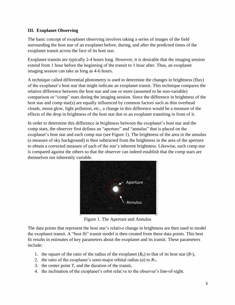
An easy way to check illumination uniformity is to make master flat frames from two sets of

images, the second set recorded after rotating the camera (or light box) by 90 degrees. Divide

one master image by the other and measure pixel intensity (ADU values) across the diagonals of

the resulting image. There will be random fluctuations due to counting statistics but ideally there

should be no systematic increase or decrease in intensity.

Figure 1. Line profiles obtained from dividing two master flats showing the result of even (left)

and uneven (right) illumination. (plots by Mark Blackford)

An example is shown in the above figure where the uneven illumination was achieved by

removing one of eight incandescent globes from the light box. The right graph shows 1%

systematic variation along diagonal 1 (blue) and 0.2% along diagonal 2 (red). When all eight

globes were used (left graph) systematic variation along diagonal 1 (blue) was less than 0.1% but

along diagonal 2 (red) it increased slightly to 0.3%.

You should aim for less than 0.5% systematic variation in illumination across your master flat

frames.

16

Appendix C:

Observation Worksheet

Exoplanet: WASP-12bObserver: Dennis Conti

Item Host Star/Exoplanet Information: (click here)1 RA: 06:30:32.792 Dec: 29:40:20.43 Period (days): 1.09144 R*: 1.635 T eff : 6300

6 Link to Reference Paper: http://www.aanda.org/articles/aa/pdf/2011/04/aa16268-10.pdf

7 Date of Observation (UT): 1/5-6/16BJD_TDB

UT (click here)8 Ingress: 1/6/2016 1:01 2457393.548749 Egress: 1/6/2016 4:01 2457393.67374

Observing Location: 10 Latitude: 38° 55' 48.51" N11 Longitude: 76° 29' 17.78" W12 Altitude (m): 013 Aperture (mm): 28014 Focal length (mm): 3010

15 CCD Camera: SX694M16 Gain (e-/ADU): 0.317 Readout noise (e-): 5.018 Dark current (e-/pixel/sec): 0.00319 Point of saturation (ADUs): 45,000

X Y20 No. of pixels (unbinned): 2750 220021 Pixel size (microns -unbinned): 4.54 4.5422 Binning: 2 223 Image scale (arcsec/pixel): 0.62 0.6224 FOV (arcmin): 14.26 11.4125 Filter: V

Limb darkening coefficients: (click here)26 Quadratic LD u1: 0.3905608127 Quadratic LD u2: 0.302699228 Exposure time (secs): 4529 FWHM (arcseconds): 2.6830 FWHM (pixels): 4

Initial Settings:31 FWHM pixel multiplier: 332 Aperture radius: 1333 Inner annulus radius: 1434 Outer annulus radius: 29

Final Settings:35 Aperture radius: 1336 Inner annulus radius: 1437 Outer annulus radius: 29

38 Original # of Science Images: 33739 Images not used: #337