AAS 17-253

LOW-THRUST MANY-REVOLUTION TRAJECTORY OPTIMIZATIONVIA DIFFERENTIAL DYNAMIC PROGRAMMING AND A SUNDMAN

TRANSFORMATION

Jonathan D. Aziz∗, Jeffrey S. Parker†, Daniel J. Scheeres‡ andJacob A. Englander§

Low-thrust trajectories about planetary bodies characteristically span a high count of orbitalrevolutions. Directing the thrust vector over many revolutions presents a challenging op-timization problem for any conventional strategy. This paper demonstrates the tractabilityof low-thrust trajectory optimization about planetary bodies by applying a Sundman trans-formation to change the independent variable of the spacecraft equations of motion to theeccentric anomaly and performing the optimization with differential dynamic programming.Fuel-optimal geocentric transfers are shown in excess of 1000 revolutions while subject toEarth’s J2 perturbation and lunar gravity.

INTRODUCTION

Highly efficient low-thrust propulsion systems enable mission designers to increase the useful spacecraftmass or delivered payload mass above that from high-thrust engine options. This improvement typicallycomes at the expense of increased times of flight to mission destinations. For low-thrust trajectories aboutplanetary bodies, an orbital period on the order of hours or days provides inadequate time to impart a sub-stantial change to the orbit and results in a large number of revolutions that are traversed before reaching thedesired state. Determining the optimal control over hundreds or thousands of revolutions poses a sensitiveand often unwieldy, high-dimensional optimization problem.

Indirect Solutions to Low-Thrust Many-Revolution Orbit Transfers

Classical approaches employ optimal control theory, named the indirect, Lagrange multiplier, or adjointmethod, beginning with Edelbaum’s transfer between circular orbits of different semi-major axis and incli-nation. Edelbaum developed an analytical solution to maximize the inclination change, ∆i, while achievinga given semi-major axis change, ∆a, between two circular orbits [1]. The result was repeated by maximiz-ing the delivered mass over a fixed transfer duration with ∆a and ∆i specified [2]. Edelbaum assumed theorbit to remain circular throughout the transfer, a constant thrust angle within each revolution, a constantthrust acceleration, and two-body dynamics. The circular orbit and constant angle assumptions are reason-ably accurate, but constant thrust acceleration is a poor model for a propellant consuming spacecraft and doesnot allow for coasting. Furthermore, a two-body dynamic model is insufficient for long duration low-thrustmissions. Wiesel and Alfano recast the problem to minimize the accumulated velocity change, ∆V , when∆a and ∆i are specified [3]. The circular orbit assumption was maintained, but a constant thrust magnitudeand mass flow rate were assumed instead of constant thrust acceleration, and the thrust angle was allowed tovary. Minimizing ∆V under these conditions similarly minimizes the transfer time and fuel consumption.

∗Ph.D. Student, Colorado Center for Astrodynamics Research, University of Colorado, Boulder, CO 80309.†Adjunct Professor, Colorado Center for Astrodynamics Research, University of Colorado, Boulder, CO 80309.‡Distinguished Professor, A. Richard Seebass Endowed Chair, Colorado Center for Astrodynamics Research, University of Colorado,Boulder, CO 80309.§Aerospace Engineer, NASA/GSFC, Code 595, 8800 Greenbelt Rd, Greenbelt, MD 20771, USA.

1

https://ntrs.nasa.gov/search.jsp?R=20170001473 2020-04-28T22:17:31+00:00Z

Wiesel and Alfano solved the resulting two point boundary value problem numerically to produce a contourmap of a constant Lagrange multiplier as a function of ∆a and ∆i. Thrust steering for the fast time scaletransfer within a single revolution is found analytically after obtaining the Lagrange multiplier from the map.For the long time scale problem, i.e. many-revolution transfers, the Lagrange multiplier is again read fromthe map, but the thrust angle expression must be approximated numerically. Kechichian reformulated Edel-baum’s transfer as a minimum-time problem and found a simple analytical expression for the time-varyingthrust angle to achieve the desired ∆a and ∆i [4].

Edelbaum extended his analysis to obtain solutions for small changes to any or all of the classical orbitalelements for elliptical orbits, again in fixed time with continuous thrust acceleration and a two-body dynamicmodel [5]. The two point boundary value problem requires numerical solution for the fast time scale transfer,but is reduced to analytical expressions for many-revolution transfers by neglecting periodic terms in theorbital element rates of change due to thrust. Kechichian obtained the adjoint equations of motion for theminimum-time rendezvous problem in non-singular equinoctial elements, and presents a numerical solutionwith Newton-Raphson iteration [6]. He suggested an orbit averaging technique to extend this result to longduration rendezvous, and followed such an approach to improve Edelbaum’s transfer to include changesin the right ascension of the ascending node, ∆Ω, and Earth’s J2 perturbation in the dynamic model [7].Kechichian further developed the low-thrust rendezvous in equinoctial elements by considering Earth zonalharmonics up to J4 [8], and shows analytical but suboptimal approaches for changing ∆a or ∆i with eclipsesincluded [9, 10].

The indirect problem is solved when Lagrange multipliers (adjoints or costates) are found to produce ad-missible states and controls that extremize the Hamiltonian at every instant in time, while obeying the stateand adjoint equations of motion and satisfying boundary and transversality conditions. Under significantassumptions, e.g. Edelbaum’s transfer, analytic expressions are found that enable quick trajectory computa-tion. Typically, however, values of the Lagrange multipliers must be guessed, evaluated in the equations ofmotion, and corrected. The evaluation and correction is iterated in a numerical procedure until optimalityconditions are satisfied. An appropriate initial guess for the Lagrange multipliers is non-intuitive and theresulting trajectory is sensitive to their values. That sensitivity is amplified when the trajectory encompassesmany revolutions. The indirect approach is further complicated by the need to reform the Hamiltonian andre-derive the adjoint equations of motion and boundary conditions as different state variables, constraints,and dynamics are considered.

Low-Thrust Control Laws

In a similar flavor to the indirect approach, control laws use just a few input parameters to describe a rulefor maneuvering a spacecraft during a transfer. The indirect solution is an optimal control law determined bythe Lagrange multipliers, but sub-optimal control laws that follow some heuristic can be particularly useful inmission design and even approach optimal results. Control laws prescribe the thrust direction and magnitudeas a function of time or angular position, for example. Spacecraft equations of motion are then evaluatedwith thrust adhering to the control law until the target orbit state is reached, but if the control law is poorlychosen, trajectory computation can proceed indefinitely. Lyapunov feedback control laws are desirable sothat convergence can be expected.

Kluever blends the results of optimal control theory for the individual minimum-time changes ∆a, ∆i andto eccentricity, ∆e, subject to two-body dynamics [11]. The control law assembles the thrust direction fromthe weighted optimal thrust directions to change each orbital element. Chang, Chichka, and Marsden suggesta Lyapunov function that is the weighted sum of squared errors of the angular momentum and Laplace vectorsbetween the current and target orbit [12]. Minimizing this Lyapunov function at each instance in time yieldsasymptotic stability for local transfers between Keplerian orbits. Chang et al. suggest transfers through afinite number of intermediate orbits for arbitrary global transfers, e.g. over many revolutions, and present amethod for choosing those intermediate orbits.

Petropolous derived analytic expressions for the optimal thrust directions and optimal orbit locations forchanging each of the classical orbital elements to propose two control law strategies that include a mechanism

2

for coasting based on the effectivity of the maneuver [13]. This work was further developed as the Q-law,where Q is a candidate Lyapunov function named the proximity quotient [14]. Q captures the proximity tothe target orbit, and best-case time-to-go for achieving the desired change in each orbital element. Thrustdirections are chosen to maximize the reduction in Q, but if the rate of reduction is below a user-specifiedvalue, the thrust is turned off. Petropolous shows a minimum-time Q-law transfer that approaches Edelbaum’sresult and the minimum-fuel case with coasting over 666 revolutions, near-optimal results with inclinationchange included and for a transfer about Vesta, and successful computation of a challenging Molniya-typetransfer.

Heuristic control laws generally yield sub-optimal trajectories, but follow a policy that a mission designerdeems acceptable. They can be particularly useful to construct an initial guess for a separate optimizationprocedure, or to estimate fuel and time of flight requirements, for example. Furthermore, the control strategycan be detached from the dynamic model. That is to say, a rule for steering can be set forth and employedwith an arbitrary set of active forces.

Direct Optimization of Low-Thrust Trajectories

While indirect methods solve for the abstract Lagrange multipliers, direct methods seek the physical vari-ables explicitly. A decision vector is formed of control variables, state variables, or other variable parametersthat collectively describe an entire trajectory. The decision vector could also be the input parameters for acontrol law. The direct optimization procedure then updates the decision vector iteratively until convergencecriteria are satisfied.

Direct optimization of heliocentric low-thrust trajectories is dominated by direct transcription and nonlin-ear programming (NLP) techniques. Direct transcription transforms the continuous optimal control probleminto a discrete approximation [15]. For example, the continuous control uptq now becomes the sequenceru0,u1, ...,uN´1s, and that sequence is the decision vector for the discretized trajectory of N stages, alsocalled grid or mesh points, or nodes. Nonlinear programming generally involves the assembly and inversionof a Hessian matrix that contains the second derivatives and cross partial derivatives of a scalar objectivefunction with respect to the decision vector. The size of the optimization problem grows quadratically withthe number of decision variables and proves to be a computational bottleneck when applying nonlinear pro-gramming to planetocentric low-thrust trajectories that require a large decision vector. Nonetheless, Bettssolved the large-scale NLP problem for geocentric trajectories over several hundred revolutions using collo-cation and sequential quadratic programming in the Sparse Optimization Suite (SOS) software [16–20]. Bettspresents a 578 revolution transfer between low Earth orbits with continuous but throttled thrust and oblateEarth perturbations through J4 [18] and a minimum time lunar transfer with two burn phases of maximumthrust and an intermediate coast phase [19]. More recently, Betts modeled coast phases for eclipse conditionsand constructed initial guesses for thrust arcs with the control law from Chang et al. An initial guess ofthe entire trajectory was constructed with a receding horizon algorithm and supplied to SOS for optimiza-tion [20]. Furthermore, the equations of motion considered oblate Earth perturbations through J4, Sun andlunar gravity perturbations, and true longitude as the independent variable. Transfers from low earth orbit togeosynchronous orbit in 248 revolutions with 363 alternating burn and coast phases and to a Molniya orbit in372 revolutions with 693 phases both maximized the delivered mass.

A linear scaling of the optimization problem size with number of control variables is characteristic ofdifferential dynamic programming (DDP) [21]. DDP solves a subproblem for each uk, k P r0, N ´ 1s inthe sequence ru0,u1, ...,uN´1s to optimize a local model of the cost remaining along the trajectory, insteadof viewing the decision vector as a whole. This is in stark contrast to methods that update the entire controlsequence in the computationally expensive matrix inverse of a large Hessian. If the control vector at eachstage is of dimension m, then DDP solves N NLP problems of size m, rather than a single NLP problem ofsize Nm.

The DDP procedure for updating the nominal control policy is called the backward sweep and is motivatedby Bellman’s Principle of Optimality.

An optimal policy has the property that whatever the initial state and initial decision are, the

3

remaining decisions must constitute an optimal policy with regard to the state resulting from thefirst decision [22].

Considering the state that results from applying the nominal control up to stage k “ N´1, the sole remainingdecision is uN´1. Optimization of this final decision is now independent of those preceding it and minimizesthe cost-to-go that is incurred along this final stage. After performing this optimization and stepping backto stage k “ N ´ 2, the remaining decisions are uN´2 and uN´1. The latter is known, however, and onlythe control at the current stage needs to be determined. An update to the entire control policy is possible byproceeding upstream to the initial state at stage k “ 0, while optimizing each stage decision along the way.

The current state-of-the-art technology for the optimal design of low-thrust planetary trajectories is theMystic Low-Thrust Trajectory Design and Visualization Software [23]. Mystic has best demonstrated itscapabilities with the success of NASA’s Dawn mission [24]. After an interplanetary leg that included a Marsgravity assist, Dawn completed its first planetary segment about the asteroid Vesta and will end its mission ina second planetary segment at the asteroid Ceres, where it currently operates. Mystic’s optimization engineis built around the Static/Dynamic Optimal Control algorithm, a DDP approach developed by Whiffen [25].Despite the favorability of DDP for large scale optimization, computation time limits Mystic to about 250revolutions for optimized trajectories before switching to the Q-law [26]. Lantoine and Russell introducedHybrid Differential Dynamic Programming (HDDP) [27–29], a DDP variant that makes the most computa-tionally expensive step suitable for parallelization.

DDP and a Sundman Transformation

This work advances the capability of differential dynamic programming applied to low-thrust spaceflightby changing the independent variable of the equations of motion. The Sundman transformation [30] is ageneral change of variables from time to a function of orbital radius, and effectively regularizes the stepsize of numerical integration [31]. Selecting the new independent variable as the eccentric anomaly is foundto add numeric stability when mapping objective function sensitivities along a trajectory, making efficientoptimization possible over hundreds of revolutions and thousands of control variables. Yam, Izzo, and Biscanipreviously applied a Sundman transformation to the Sim-Flanagan transcription to optimize interplanetarytrajectories [32, 33]. Pellegrini, Russell, and Vivek show accuracy and efficiency gains for propagation withthe Sundman transformation in the Stark and Kepler models [34].

Presentation begins with the state and dynamic model used to compute example trajectories. Next, thegeneralized Sundman transformation is provided with a derivation for the change of variable to eccentricanomaly. The optimization problem is then posed, and the procedure for computing trajectories is detailed.Implementation closely follows the procedure outlined by the HDDP algorithm [27], so presentation of thealgorithm is withheld. Results for the Sundman-transformed DDP approach follow in the form of an exampleorbit transfer solved for different cases of increasing complexity.

PROBLEM FORMULATION

Fuel-optimal low-thrust transfers from geostationary transfer orbit (GTO) to geosynchronous orbit (GEO)are computed to demonstrate the efficacy of the Sundman-transformed DDP approach.

Spacecraft State and Dynamics

The spacecraft state is chosen as a Cartesian representation of the spacecraft inertial position and velocity.

r “ rx y zsT, v “ r 9x 9y 9zs

T (1)

Henceforth, boldface is reserved for column vectors and an overhead dot denotes the time derivative. Imple-mentation of the HDDP algorithm makes use of an augmented state vector that includes time t, mass m, andthrust control variables T , α, and β.

X “ rt x y z 9x 9y 9z m T α βsT (2)

4

Table 1: Dynamic Model Parameters.

µ‘ 398600.44 km3/s2 Tmax 0.25 N

µK 4904.928372 km3/s2 Isp 1950 s

J2 0.0010826265 g0 0.00980665 km/s2

R‘ 6378.136 km

Spherical thrust control is defined by magnitude T , yaw angle α, and pitch angle β, where the angles aredefined relative to the radial-transverse-normal (RSW) frame. RSW basis vectors and thus the rotation to theinertial frame are defined by,

rr s ws “

„

r

r

pr ˆ vq ˆ r

‖pr ˆ vq ˆ r‖r ˆ v

‖r ˆ v‖

. (3)

Thrust vector components are then«

TrTsTw

ff

“

«

T sinα cosβT cosα cosβT sinβ

ff

,

«

TxTyTz

ff

“ rr s ws

«

TrTsTw

ff

, (4)

so that the pitch angle is measured from the orbit plane about the radial direction and the yaw angle is mea-sured from the transverse direction about the angular momentum. No concern is given for angle wrapping.In fact, computation exhibits favorable performance when the angles are unbounded. Spacecraft dynamicsconsider geocentric two-body motion perturbed by thrust, J2, and lunar gravity,

9X “ 9X‘ ` 9XT ` 9XJ2` 9XK, (5)

where 9X‘ is the two-body motion due to point mass Earth gravity, 9XT is the thrust acceleration and massflow rate, 9XJ2

is Earth’s J2 perturbation, and 9XK is the point mass lunar gravity perturbation, defined by,

9X‘ “

”

1 9x 9y 9z ´µ‘r3x ´

µ‘r3y ´

µ‘r3z 0 0 0 0

ıT

, (6a)

9XT “

„

0 0 0 0Txm

Tym

Tzm

´T

Ispg00 0 0

T

, (6b)

9XJ2“ ´

3J2µ‘R2‘

2r5

„

0 0 0 0 xp1´ 5z2

r2q yp1´ 5

z2

r2q zp3´ 5

z2

r2q 0 0 0 0

T

, (6c)

9XK “ ´µK

„

0 0 0 0x´ xK

‖r ´ rK‖3`xK

rK3

y ´ yK

‖r ´ rK‖3`

yK

rK3

z ´ zK

‖r ´ rK‖3`

zK

rK3

0 0 0 0

T

.

(6d)

Gravitational parameters for the Earth and the Moon are µ‘ and µK, respectively. A constant power model isassumed with T P r0, Tmaxs. Thrust magnitude constraints are enforced by a null-space method [28]. Massflow rate is inversely proportional to the specific impulse, Isp, and acceleration due to gravity at sea level g0.The J2 perturbation is owed to the Earth’s oblateness, and is a function of the Earth’s equatorial radius R‘.Table 1 lists these dynamic model constants. Including the lunar perturbation requires the Moon’s inertialposition with respect to the Earth,

rK “ rxK yK zKsT, (7)

that is assumed to evolve according to geocentric two-body motion. The Moon’s state is initialized with theorbital elements listed in Table 2, where ω and M are introduced as the argument of periapsis and meananomaly.

5

Table 2: The Moon’s Earth-Centered ICRF Orbital Elements at 01 Jan 2000 00:00:00.0 TDB.

a 381218.68756119191 km Ω 12.23324045627363˝

e 0.06476694126942699 ω 60.7835754956735˝

i 20.94024252661913˝ M 140.7402558848975˝

A 2000 kg spacecraft is initialized at the J2000 epoch on the x-axis with the position and velocity selectedfor an example GTO with approximately 300 km perigee altitude and 28.5˝ inclination.

X0 “

»

—

—

—

—

—

—

—

—

—

—

—

–

t0x0y0z09x09y09z0m0T0α0β0

fi

ffi

ffi

ffi

ffi

ffi

ffi

ffi

ffi

ffi

ffi

ffi

fl

“

»

—

—

—

—

—

—

—

—

—

—

—

–

01 Jan 2000 12:00:00.0 TDB6678.1363 km

000

8.92130624172 km/s4.84387407216 km/s

2000 kg000

fi

ffi

ffi

ffi

ffi

ffi

ffi

ffi

ffi

ffi

ffi

ffi

fl

(8)

Equation 8 is the spacecraft initial state vector. The initial time is listed as the J2000 epoch, but state variablet is numerically integrated to track the relative time from t0 “ 0. An initial guess for the controls must beprovided along the entire trajectory. Those controls are identically zero at all times as shown for the initialstate.

Sundman Transformation

In regularizing the equations of motion to solve the three-body problem, Karl Sundman introduced a changeof independent variable from time to the new independent variable τ [30].

dt “ cnrndτ (9)

Time and the new independent variable are related by a function of the orbital radius. The real number n andcoefficient cn may be selected so that τ represents an orbit angle. Transforming the time-dependent equa-tions of motion simply requires a multiplication by the functional relationship between the two independentvariables.

X “

ˆ

d

dtX

˙

dt

dτ“ 9Xcnr

n (10)

Time-dependent equations of motion are typically propagated for a prescribed duration from the state at aninitial epoch. Now however, propagation is specified for a duration of τ and the elapsed time is unknown apriori. Time may be tracked by including it in the state vector.

The Sundman transformation to eccentric anomaly is found by differentiating Kepler’s equation,

t “a

a3µ pE ´ e sinEq , (11)

dt “a

a3µ p1´ e cosEqdE “ cnrndτ , (12)

where E is the eccentric anomaly. Considering n “ 1 and making use of the relationship r “ ap1´ e cosEqleads to a solution for c1.

c1 “ p1rqa

a3µ p1´ e cosEq “ p1rqa

a3µ praq “a

aµ (13)

dt “a

aµ rdE (14)

6

Sundman Transformed Dynamics

The Sundman transformation is made after assembling the complete equations of motion with respect totime.

X “ p 9X‘ ` 9XT ` 9XJ2 `9XKq

a

aµ‘ r (15)

HDDP makes use of the first-order state transition matrix (STM) and second-order state transition tensor(STT) to map cost function derivatives between stages. Differential equations for the STMs (referring to boththe STMs and STTs) rely on the dynamics matrix and tensor,

Ai,j “B 9Xi

BXj, (16a)

Ai,jk “B2 9Xi

BXjBXk, (16b)

where tensor notation has been adopted to avoid ambiguities. The dynamics matrix and tensor similarly needto be transformed to reflect the change of independent variable.

Λi,j “BXi

BXj(17a)

Λi,jk “B2Xi

BXjBXk(17b)

The new dynamics matrix and tensor in Equations (17a) and (17b) are similarly obtained first with respectto time and then the change of variables is performed by extensive application of the chain rule. First, thegeneral Sundman transformation is redefined along with its first and second derivatives with respect to thestate vector.

η “ dtdτ “ cnrn (18)

ηXi “

Bη

BXi(19)

ηXXi,j “

B2η

BXiBXj(20)

After assembling Equations (16a) and (16b), the chain rule completes the transformation.

Λi,j “ Ai,jη ` 9XiηXj (21a)

Λi,jk “ Ai,jkη `Ai,jηXk `Ai,kηX

j ` 9XiηXXj,k (21b)

Equations (18) to (21) are stated generally for any change of independent variable, but τ is selected as theeccentric anomaly for the computed examples.

Augmented Lagrangian Method

The standard DDP formulation adjoins terminal constraints ψpXf q “ 0 to the original cost function usinga constant vector of Lagrange multipliers. HDDP selects a cost function based on the augmented Lagrangianmethod where a scalar penalty parameter places additional weight on terminal constraint violations. Here apenalty matrix is used so that the additional weight on each constraint can be treated individually.

J “ φ` λTψ `ψTΣψ (22)

The first term φpXf q is the original objective to be minimized, where Xf is the final value of the statevector. Multipliers λ are initialized as the zero vector and updated at every iteration to push the trajectorytoward feasibility. Penalty matrix Σ places additional weight on constraint violations and serves to initializea quadratic cost function space. In contrast to previous approaches that continually increase the penalty

7

weight [27, 35], Σ is held constant for all iterations. In practice, the entries of Σ are tuned after observinghow the iterates progress toward feasibility. For example, an initial attempt to optimize a trajectory mightbegin with Σ as a scalar multiple of the identity matrix so that each constraint is weighted equally. If iteratesshow little progress toward satisfying a particular constraint, its associatedΣ entry could be increased and theprocess restarted. Similarly, if the algorithm appears to prioritize a constraint without working to satisfy theother constraints, theΣ entry for that prioritized constraint could be reduced. The initial guess of zero-valuedmultipliers is not a requirement and may also be viewed as tuning parameters.

Final conditions for GEO are described in the terminal constraint function ψ, so that ψpXf q “ 0 for afeasible solution. The objective is to arrive at GEO after expending the minimum amount of propellant.

φ “ ´mf (23a)

ψ “

»

—

—

–

‖rf‖´ 42164.169972 km‖vf‖´ 3.07466008566 km/s

rf ¨ vfzf9zf

fi

ffi

ffi

fl

(23b)

Σ “ diagpσ0, σ1, σ3, σ4q (23c)

The terminal constraint function is satisfied upon arrival at GEO distance with circular orbital velocity, zeroflight path angle and zero inclination. The arrival longitude is unconstrained. The penalty matrix placesadditional weight on the final position and velocity magnitude constraints, and its entries are later specifiedfor each computed example. A scaled feasibility tolerance requires ‖ψ‖ ă 1 ˆ 10´6 and an optimalitytolerance requires ER0 ă 1ˆ 10´7, where ER0 is the expected reduction of the objective function obtainedin the backward sweep [27]. Then the constraint violations are satisfactorily small and the backward sweepsees a stationary point of the cost function with respect to controls and multipliers. Scaling improves thenumerical stability of the procedures but adds to the set of tuning parameters. Here a distance unit DU , timeunit TU , force unit FU , and mass unit MU are set as

DU “ 42164.0 km

TU “ 10

b

DU3µ‘

FU “ 0.25 N

MU “ FU TU2DU

, (24)

where the distance unit is approximately GEO radius, the time unit has been scaled by an additional factorof 10, and the force unit is the maximum thrust. The scaled feasibility tolerance corresponds to a 42.164 mposition requirement and 0.3075 mm/s velocity requirement.

Trajectory Computation

HDDP considers a discrete form of DDP where a trajectory can be described by any number of phases,with each phase described by a number of stages. This work considers single phase trajectories of N stages.The trajectory computation step is named the forward pass, and is the sequence of function evaluations,

Xk`1 “ F pXkq, k “ 0, 1, ..., N ´ 1. (25)

The transition function F dictates how the state evolves between stages, and might obey a system of linear,nonlinear, or differential equations, and is not necessarily deterministic. DDP is applicable to all of these sys-tems in both continuous and discrete form [21]. The relevant transition function is the integral of Equation 15between stages.

Xk`1 “Xk `

Ek`1ż

Ek

Xk dE (26)

8

Propagating a trajectory from the initial state requires effective discretization and a numerical integrationscheme. Equation 26 is integrated with a fixed-step fifth-order Dormand-Prince method [36]. The trajectoryis described by 100 stages per revolution that are equally spaced in eccentric anomaly. There are then 300control variables for every revolution. Each stage offers an opportunity to update the thrust control variablesthat are held constant across an integration step.

A fixed integration step accumulates ∆E “ Ek`1 ´ Ek “ 2π100. Having set the initial guess for allstage control variables to zero, the first iteration considers a ballistic orbit in GTO for a prescribed number ofrevolutions, Nrev. The fixed transfer duration in eccentric anomaly is 2πNrev.

STM Computation

Results were generated on a Dual Intel Xeon quad-core 2GHz, 24GB memory Linux machine. STMcomputations were distributed in parallel across 8 cores with OpenMP [37]. All other steps of the algorithmrun serially. To permit parallelization, STMs are obtained separately from attempted trajectories with trialcontrols. When an iterate is accepted as the new nominal trajectory, Equation 26 is augmented with the STMdifferential equations.

Φi,j “ Λi,aΦa,j (27a)

Φi,jk “ Λi,aΦa,jk ` Λi,abΦa,jΦb,k (27b)

STMs are initialized as Φi,j “ δi,j and Φi,jk “ 0. Equation 27 is stated in terms of the Sundman transfor-mation, but all that changes from the time-dependent case is the notation. EachXk is known, so integrationsfrom any stage k to k ` 1 can be performed separately and in parallel, instead of serially from k “ 0 tok “ N ´ 1.

RESULTS

Four example trajectories are computed from initial conditions in Equation 8, and with HDDP employedto minimize the augmented Lagrangian described in Equations (22) and (23). First, only two-body dynamicsare considered, so that Equation 15 ignores the J2 and lunar gravity perturbations. The J2 perturbationis introduced in the second case, while the third and fourth cases include both perturbations. The transferduration is fixed at Nrev “ 450.5 for the first three cases, and Nrev “ 1000.5 for the final case. The penaltymatrix is initially tuned to Σ “ diagp100, 10, 1, 1, 1q.

Case 1: 450.5 Revolutions With 2-Body Dynamics

The first example spans 450.5 revolutions, yielding 135,150 control variables to compute. In the 2-bodydynamic model, the spacecraft acceleration is due to point-mass Earth gravity and thrust. The choice ofNrev “ 450.5 is somewhat arbitrary but allows quick computation of a many-revolution trajectory with alarge number of control switches between thrust and coast arcs. Prescribing the extra half-revolution fixes theterminal state of the initial guess to be at apogee on the negative x-axis.

Figure 1 provides a two-dimensional view of the resulting transfer in the equatorial plane and the steeringprofile for both thrust angles. After 450.5 revolutions, 315.75 days have elapsed and the spacecraft arrives inGEO with a final mass of 1759.1754 kg. The eccentricity vector and line of nodes remain coincident through-out the transfer, yielding symmetry in the pitch and yaw steering to remove the eccentricity and inclination.Apogee raising early in the transfer is leveraged for a cheaper inclination change. Both Figures 1 and 2 showhow a long initial maneuver is followed by the bang-bang thrust profile expected for a fuel-optimal transfer.Yaw steering is symmetric about the transverse direction and switches sign at the apsides. Pitch steering tochange the inclination is favored around apogee. Both pitch and yaw are zero-valued for coast arcs, which isnot arbitrary, because this sets the nominal value for a control update during iteration. Given the definitionsof α and β in Equation 4, if an iterate attempts to turn the thrust on, that initial thrust increment must stepfrom the positive transverse and/or normal directions.

9

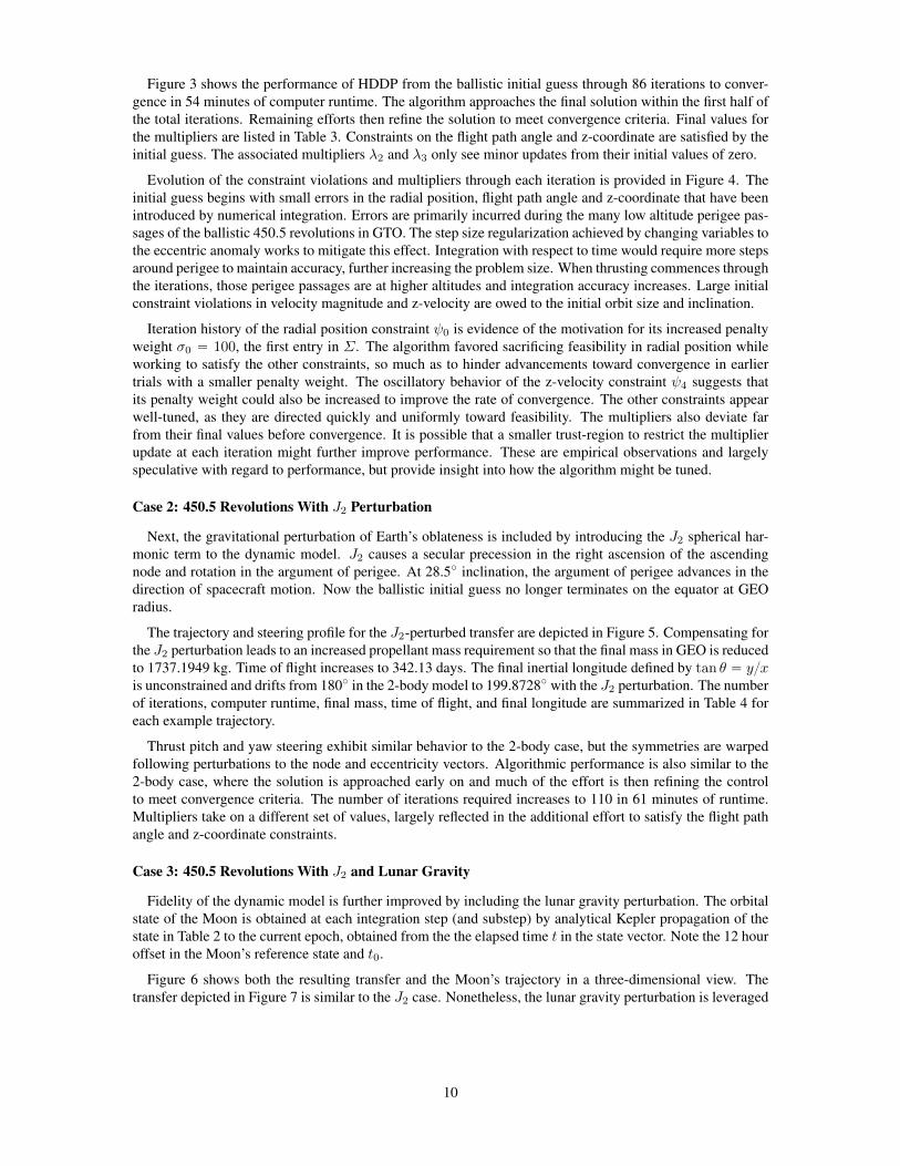
Figure 3 shows the performance of HDDP from the ballistic initial guess through 86 iterations to conver-gence in 54 minutes of computer runtime. The algorithm approaches the final solution within the first half ofthe total iterations. Remaining efforts then refine the solution to meet convergence criteria. Final values forthe multipliers are listed in Table 3. Constraints on the flight path angle and z-coordinate are satisfied by theinitial guess. The associated multipliers λ2 and λ3 only see minor updates from their initial values of zero.

Evolution of the constraint violations and multipliers through each iteration is provided in Figure 4. Theinitial guess begins with small errors in the radial position, flight path angle and z-coordinate that have beenintroduced by numerical integration. Errors are primarily incurred during the many low altitude perigee pas-sages of the ballistic 450.5 revolutions in GTO. The step size regularization achieved by changing variables tothe eccentric anomaly works to mitigate this effect. Integration with respect to time would require more stepsaround perigee to maintain accuracy, further increasing the problem size. When thrusting commences throughthe iterations, those perigee passages are at higher altitudes and integration accuracy increases. Large initialconstraint violations in velocity magnitude and z-velocity are owed to the initial orbit size and inclination.

Iteration history of the radial position constraint ψ0 is evidence of the motivation for its increased penaltyweight σ0 “ 100, the first entry in Σ. The algorithm favored sacrificing feasibility in radial position whileworking to satisfy the other constraints, so much as to hinder advancements toward convergence in earliertrials with a smaller penalty weight. The oscillatory behavior of the z-velocity constraint ψ4 suggests thatits penalty weight could also be increased to improve the rate of convergence. The other constraints appearwell-tuned, as they are directed quickly and uniformly toward feasibility. The multipliers also deviate farfrom their final values before convergence. It is possible that a smaller trust-region to restrict the multiplierupdate at each iteration might further improve performance. These are empirical observations and largelyspeculative with regard to performance, but provide insight into how the algorithm might be tuned.

Case 2: 450.5 Revolutions With J2 Perturbation

Next, the gravitational perturbation of Earth’s oblateness is included by introducing the J2 spherical har-monic term to the dynamic model. J2 causes a secular precession in the right ascension of the ascendingnode and rotation in the argument of perigee. At 28.5˝ inclination, the argument of perigee advances in thedirection of spacecraft motion. Now the ballistic initial guess no longer terminates on the equator at GEOradius.

The trajectory and steering profile for the J2-perturbed transfer are depicted in Figure 5. Compensating forthe J2 perturbation leads to an increased propellant mass requirement so that the final mass in GEO is reducedto 1737.1949 kg. Time of flight increases to 342.13 days. The final inertial longitude defined by tan θ “ yxis unconstrained and drifts from 180˝ in the 2-body model to 199.8728˝ with the J2 perturbation. The numberof iterations, computer runtime, final mass, time of flight, and final longitude are summarized in Table 4 foreach example trajectory.

Thrust pitch and yaw steering exhibit similar behavior to the 2-body case, but the symmetries are warpedfollowing perturbations to the node and eccentricity vectors. Algorithmic performance is also similar to the2-body case, where the solution is approached early on and much of the effort is then refining the controlto meet convergence criteria. The number of iterations required increases to 110 in 61 minutes of runtime.Multipliers take on a different set of values, largely reflected in the additional effort to satisfy the flight pathangle and z-coordinate constraints.

Case 3: 450.5 Revolutions With J2 and Lunar Gravity

Fidelity of the dynamic model is further improved by including the lunar gravity perturbation. The orbitalstate of the Moon is obtained at each integration step (and substep) by analytical Kepler propagation of thestate in Table 2 to the current epoch, obtained from the the elapsed time t in the state vector. Note the 12 houroffset in the Moon’s reference state and t0.

Figure 6 shows both the resulting transfer and the Moon’s trajectory in a three-dimensional view. Thetransfer depicted in Figure 7 is similar to the J2 case. Nonetheless, the lunar gravity perturbation is leveraged

10

(a) (b)

(c) (d)

Figure 1: An equatorial projection of the 450.5 revolution transfer from GTO to GEO with 2-body dynamicsis colored by (a) yaw angle contours and (b) pitch angle contours with coast arcs in blue. Markers are placedat the initial and final states and a dashed line marks the target GEO orbit. (c) Thrust yaw angle and (d) pitchangle are shown for the duration of the transfer.

11

(a) (b)

Figure 2: Thrust magnitude through the 450.5 revolution transfer from GTO to GEO with 2-body dynamicsfor (a) the full mission duration and (b) a zoom on the final days to emphasize the bang-bang control structure.

Figure 3: Iteration history of the scaled cost function, the final mass in kilograms, the scaled cost contri-butions from the multiplier term and the scaled norm of the constraint violations for the 450.5 revolutiontransfer from GTO to GEO with 2-body dynamics.

12

Figure 4: Iteration history of the scaled constraints and multipliers for the 450.5 revolution transfer fromGTO to GEO with 2-body dynamics.

13

(a) (b)

(c) (d)

Figure 5: An equatorial projection of the 450.5 revolution transfer from GTO to GEO with 2-body dynamicsand Earth’s J2 perturbation is colored by (a) yaw angle contours and (b) pitch angle contours with coast arcsin blue. Markers are placed at the initial and final states and a dashed line marks the target GEO orbit.(c) Thrust yaw angle and (d) pitch angle are shown for the duration of the transfer.

14

(a) (b)

Figure 6: A three dimensional perspective of the 450.5 revolution transfer from GTO to GEO with 2-bodydynamics perturbed by Earth J2 lunar gravity (a) shows the trajectory of the Moon and (b) a closer view,colored according to thrust yaw angle.

to improve the final mass to 1745.2012 kg. The resulting time of flight is 322.63 days and final longitude is201.0805˝. Multipliers are similar to the J2 case with the exception of λ0, the multiplier associated with theorbital radius constraint.

An additional 25 iterations from the J2 case are required to compute the transfer, coincidentally the sameincrease from the 2-body case to J2 case. However, computer runtime sees a worse penalty. The increase to107 minutes is owed largely to computing the Moon’s orbital state in the forward pass and its derivatives inthe STMs. With time included in the augmented state vector, the associated entries in the dynamics matrixand tensor include the Moon’s velocity and acceleration.

Case 4: 1000.5 Revolutions With J2 and Lunar Gravity

A final example maintains the J2 and lunar gravity perturbed model, but increases the transfer duration to1000.5 revolutions. Now there are 300,150 optimization variables. Reducing the penalty matrix entry σ0, theweight on the orbital radius constraint, was found to improve performance.

Σ “ diagp10, 10, 1, 1, 1q (28)

Perigee thrust arcs that were characteristic of the earlier transfers do not arise. Iterates did not deviate farfrom the target orbital radius to achieve a cheaper inclination change, so the higher penalty weight wasunwarranted.

Time of flight increases with the number of revolutions to 558.86 days. The increased duration allows formore thrust arcs that are condensed around their optimal locations. The resulting final mass increases beyondthat of even the 2-body case to 1784.3632 kg. Of course, the increased transfer time also allows for moreprecession in argument of perigee. The final longitude drifts to 276.7209˝.

Thrust angle profiles in Figure 8 depict a 76 day coast arc that begins 105 days into the transfer, indicatingthat fixing the transfer to 1000.5 revolutions has over-prescribed the number of revolutions required. Pitchand yaw steering exhibit different behavior on either side of this long coast arc.

The number of iterations required has increased along with the problem size up to 913. Total cost andmultiplier contributions λTψ evolve similarly to the previous cases, but the mass and feasibility history in

15

(a) (b)

(c) (d)

Figure 7: An equatorial projection of the 450.5 revolution transfer from GTO to GEO with 2-body dynamicsperturbed by Earth J2 and lunar gravity is colored by (a) yaw angle contours and (b) pitch angle contourswith coast arcs in blue. Markers are placed at the initial and final states and a dashed line marks the targetGEO orbit. (c) Thrust yaw angle and (d) pitch angle are shown for the duration of the transfer.

16

(a) (b)

(c) (d)

Figure 8: An equatorial projection of the 1000.5 revolution transfer from GTO to GEO with 2-body dynam-ics perturbed by Earth J2 and lunar gravity is colored by (a) yaw angle contours and (b) pitch angle contourswith coast arcs in blue. Markers are placed at the initial and final states and a dashed line marks the targetGEO orbit. (c) Thrust yaw angle and (d) pitch angle are shown for the duration of the transfer.

Figure 9 suggest a step toward an intermediate solution that could not meet feasibility requirements.

The increase in computation time with problem size jumps an order of magnitude for the 1000.5 revolutioncase up to nearly 1 day from runtimes of 1-2 hours for the shorter cases. While the number of controlvariables grows linearly, there is no guarantee for the effect on convergence properties as the spacecrafttrajectory problem is nonlinear and the algorithm is sensitive to tuning. A super-linear but less than quadraticincrease in computational effort should be expected.

Computer memory requirements are driven by storage of the state and STMs. At each stage there are 11state components, 112 STM components, and 113 STT components. Storing 8-byte values for 100 stages perrevolution, across 1000.5 revolutions, requires 1.17 GB. Ignoring the possible savings from symmetry andsparsity patterns, the 3ˆ 3 control Hessians for each stage require just 7.2 MB, whereas a single Hessian forall 300,150 control variables would require 720.72 GB.

17

Figure 9: Iteration history of the scaled cost function, the final mass in kilograms, the scaled cost contri-butions from the multiplier term and the scaled norm of the constraint violations for the 1000.5 revolutiontransfer from GTO to GEO with 2-body dynamics perturbed by Earth J2 and lunar gravity.

Table 3: Multipliers for Example Cases.

Perturbations Nrev λ0 λ1 λ2 λ3 λ4

None 450.5 0.4874 -0.4205 5.4191 ˆ10´4 -2.8552 ˆ10´3 -0.2470

J2 450.5 3.2181 -0.2713 -0.1157 -4.2530 -0.1756

J2 and Lunar Gravity 450.5 0.9317 -0.2790 -0.0752 -2.9954 -0.1191

J2 and Lunar Gravity 1000.5 -0.3183 -0.3045 -0.0874 -0.0153 0.1486

Table 4: Summary of GTO to GEO Results.

Perturbations Nrev Iterations Runtime (minutes) mf (kg) tf (days) θ (deg)

None 450.5 86 54 1759.1754 315.75 180.0

J2 450.5 111 61 1737.1949 342.13 199.8728

J2 and Lunar Gravity 450.5 136 107 1745.3012 322.63 201.0805

J2 and Lunar Gravity 1000.5 913 1359 1784.3632 558.86 276.7209

18

CONCLUSION

This paper presents an approach to the low-thrust many-revolution spacecraft trajectory optimization prob-lem. Differential dynamic programming is well-suited for high-dimensional problems and the hybrid dif-ferential dynamic programming algorithm has been implemented as the optimization procedure. Posing thespacecraft trajectory problem with a dependency on eccentric anomaly instead of time is accomplished viathe Sundman transformation. Application of HDDP to the Sundman-transformed problem exhibits practicalperformance for challenging trajectories that are otherwise intractable for common approaches. The utility ofthis method has been demonstrated by a set of transfers from geostationary transfer orbit to geosynchronousorbit in 450.5 revolutions for dynamic models of increasing fidelity and finally for a 1000.5 revolution trans-fer.

The trajectories that have been presented should be viewed as local solutions for the given problem setup.A large set of tuning parameters must be selected. Different sets of scaling factors, penalty weights, andimplementation in general will affect how the iterates advance toward different local optima. Discretizationcould be refined or relaxed, and the control more or less sophisticated.

This approach is amenable to different Sundman tranformations, thrust representations, and dynamic mod-els. One can simply “plug in” the choice of each, given that the required first and second derivatives areavailable. Real-world mission design is then practical with models of a true propulsion system and truedynamics.

ACKNOWLEDGMENT

This work was supported by a NASA Space Technology Research Fellowship.

REFERENCES

[1] T. Edelbaum, “Propulsion Requirements for Controllable Satellites,” ARS Journal, Vol. 31, August1961, pp. 1079–1089.

[2] T. Edelbaum, “Theory of Maxima and Minima,” Optimization Techniques, With Applications toAerospace Systems, 1962.

[3] W. E. Wiesel and S. Alfano, “Optimal Many-Revolution Orbit Transfer,” Journal of Guidance, Control,and Dynamics, Vol. 8, 1985, pp. 155–157.

[4] J. A. Kechichian, “Reformulation of Edelbaum’s Low-Thrust Transfer Problem Using Optimal ControlTheory,” Journal of Guidance, Control, and Dynamics, Vol. 20, September 1997, pp. 988–994.

[5] T. N. Edelbaum, “Optimum Low-Thrust Rendezvous and Station Keeping,” AIAA Journal, Vol. 2, No. 7,1964, pp. 1196–1201.

[6] J. A. Kechichian, “Optimal Low-Thrust Rendezvous Using Equinoctial Orbit Elements,” Acta Astro-nautica, Vol. 38, No. 1, 1996, pp. 1–14.

[7] J. A. Kechichian, “Optimal Low-Thrust Transfer in General Circular Orbit Using Analytic Averaging ofthe System Dynamics,” The Journal of the Astronautical Sciences, Vol. 57, January-June 2009, pp. 369–392.

[8] J. A. Kechichian, “Inclusion of Higher Order Harmonics in the Modeling of Optimal Low-Thrust OrbitTransfer,” The Journal of the Astronautical Sciences, Vol. 56, January-March 2008, pp. 41–70.

[9] J. A. Kechichian, “Orbit Raising with Low-Thrust Tangential Acceleration in Presence of EarthShadow,” Journal of Spacecraft and Rockets, Vol. 35, July-August 1998, pp. 516–525.

[10] J. A. Kechichian, “Low-Thrust Inclination Control in Presence of Earth Shadow,” Journal of Spacecraftand Rockets, Vol. 35, July-August 1998, pp. 526–532.

[11] C. A. Kluever, “Simple Guidance Scheme for Low-Thrust Orbit Transfers,” Journal of Guidance, Con-trol, and Dynamics, Vol. 21, November 1998, pp. 1015–1017.

[12] D. E. Chang, D. F. Chichka, and J. E. Marsden, “Lyapunov-Based Transfer Between Elliptic KeplerianOrbits,” Discrete and Continuous Dynamical Systems-Series B, Vol. 2, February 2002, pp. 57–67.

[13] A. E. Petropoulos, “Simple Control Laws for Low-Thrust Orbit Transfers,” AAS/AIAA AstrodynamicsSpecialist Conference, August 2003.

[14] A. E. Petropoulos, “Low-Thrust Orbit Transfers Using Candidate Lyapunov Functions with a Mecha-nism for Coasting,” AIAA/AAS Astrodynamics Specialist Conference and Exhibit, August 2004.

19

[15] J. T. Betts, “Practical Methods for Optimal Control and Estimation using Nonlinear Programming,”Society for Industrial and Applied Mathematics, 2010.

[16] J. T. Betts, “Trajectory Optimization Using Sparse Sequential Quadratic Programming,” Optimal con-trol, International Series of Numerical Mathematics (R. Bulirsch, A. Miele, J. Stoer, and K. Well, eds.),Vol. 117, Birkhauser Basel, 1993.

[17] J. T. Betts, “Sparse Optimization Suite, SOS, User’s Guide, Release 2015.11,” http://www.appliedmathematicalanalysis.com/downloads/sosdoc.pdf. [Online; accessed November-2016].

[18] J. T. Betts, “Very Low-Thrust Trajectory Optimization Using a Direct SQP Method,” Journal of Com-putational and Applied Mathematics, Vol. 120, August 2000, pp. 27–40.

[19] J. T. Betts and S. O. Erb, “Optimal Low Thrust Trajectories to the Moon,” SIAM Journal on AppliedDynamical Systems, Vol. 2, May 2003, pp. 144–170.

[20] J. T. Betts, “Optimal Low Thrust Orbit Transfers with Eclipsing,” Optimal Control Applications andMethods, Vol. 36, February 2014.

[21] D. H. Jacobson and D. Q. Mayne, “Differential Dynamic Programming,” American Elsevier PublishingCompany, Inc., 1970.

[22] R. E. Bellman, “Dynamic Programming,” Princeton University Press, 1957.[23] N. T. T. Program, “Mystic Low-Thrust Trajectory Design and Visualization Software,” https://software.

nasa.gov/software/NPO-43666-1. [Online; accessed October-2016].[24] M. D. Rayman, T. C. Fraschetti, C. A. Raymond, and C. T. Russell, “Dawn: A mission in development

for exploration of main belt asteroids Vesta and Ceres,” Acta Astronautica, Vol. 58, April 2006, pp. 605–616.

[25] G. J. Whiffen, “Static/Dynamic Control for Optimizing a Useful Objective,” No. Patent 6496741, De-cember 2002.

[26] G. J. Whiffen, “Mystic: Implementation of the Static Dynamic Optimal Control Algorithm for High-Fidelity, Low-Thrust Trajectory Design,” AIAA/AAS Astrodynamics Specialist Conference and Exhibit,August 2006.

[27] G. Lantoine and R. P. Russell, “A Hybrid Differential Dynamic Programming Algorithm for ConstrainedOptimal Control Problems. Part 1: Theory,” Journal of Optimization Theory and Applications, Vol. 154,No. 2, 2012, pp. 382–417.

[28] G. Lantoine and R. P. Russell, “A Hybrid Differential Dynamic Programming Algorithm for ConstrainedOptimal Control Problems. Part 2: Application,” Journal of Optimization Theory and Applications,Vol. 154, No. 2, 2012, pp. 418–442.

[29] G. Lantoine and R. P. Russell, “A Methodology for Robust Optimization of Low-Thrust Trajectories inMulti-Body Environments,” Ph.D. Thesis, 2010.

[30] K. Sundman, “Memoire sur le probleme des trois corps,” Acta Math, Vol. 36, 1913, pp. 105–179,doi:10.1007/BF02422379.

[31] G. Jannon and V. R. Bond, “The Elliptic Anomaly,” NASA Technicai Memorandum 58228, April 1980.[32] C. H. Yam, D. D. Lorenzo, and D. Izzo, “Towards a High Fidelity Direct Transcription Method for

Optimisation of Low-Thrust Trajectories,” International Conference on Astrodynamics Tools and Tech-niques - ICATT, 2010.

[33] J. A. Sims and S. N. Flanagan, “Preliminary Design of Low-Thrust Interplanetary Missions,” AAS/AIAAAstrodynamics Specialist Conference, August 1999.

[34] E. Pellegrini, R. P. Russell, and V. Vittaldev, “F and G Taylor Series Solutions to the Stark and Keplerproblems with Sundman Transformations,” Celestial Mechanics and Dynamical Astronomy, Vol. 118,April 2014, pp. 355–378.

[35] J. D. Aziz, J. S. Parker, and J. A. Englander, “Hybrid Differential Dynamic Programming With Stochas-tic Search,” AAS/AIAA Space Flight Mechanics Meeting, February 2016.

[36] P. Prince and J. Dormand, “High order embedded Runge-Kutta formulae,” Journal of Computationaland Applied Mathematics, Vol. 7, Issue 1, March 1981, pp. 67–75.

[37] O. A. R. Board, “OpenMP Application Program Interface Version 3.0,” May 2008.

20