Aalborg Universitet Robust Computation of Error Vector ...

Aalborg Universitet

Robust Computation of Error Vector Magnitude for Wireless Standards

Jensen, Tobias Lindstrøm; Larsen, Torben

Published in:I E E E Transactions on Communications

DOI (link to publication from Publisher):10.1109/TCOMM.2012.022513.120093

Publication date:2013

Document VersionEarly version, also known as pre-print

Link to publication from Aalborg University

Citation for published version (APA):Jensen, T. L., & Larsen, T. (2013). Robust Computation of Error Vector Magnitude for Wireless Standards. I E EE Transactions on Communications, 61(2), 648-657. https://doi.org/10.1109/TCOMM.2012.022513.120093

General rightsCopyright and moral rights for the publications made accessible in the public portal are retained by the authors and/or other copyright ownersand it is a condition of accessing publications that users recognise and abide by the legal requirements associated with these rights.

- Users may download and print one copy of any publication from the public portal for the purpose of private study or research. - You may not further distribute the material or use it for any profit-making activity or commercial gain - You may freely distribute the URL identifying the publication in the public portal -

Take down policyIf you believe that this document breaches copyright please contact us at [email protected] providing details, and we will remove access tothe work immediately and investigate your claim.

Downloaded from vbn.aau.dk on: March 16, 2022

https://doi.org/10.1109/TCOMM.2012.022513.120093

https://vbn.aau.dk/en/publications/9bbad2af-c31f-40de-ac98-5f020a43316d

https://doi.org/10.1109/TCOMM.2012.022513.120093

ACCEPTED FOR PUBLICATION: IEEE TRANS. ON COMMUNICATIONS 1

Robust Computation of Error Vector Magnitude

for Wireless Standards

Tobias L. Jensen & Torben Larsen, Senior Member, IEEE

Abstract

The modulation accuracy described by an error vector magnitude is a critical parameter in modern

communication systems — defined originally as a performance metric for transmitters but now also

used in receiver design and for more general signal analysis. The modulation accuracy is a measure

of how far a test signal is from a reference signal at the symbol values when some parameters in a

reconstruction model are optimized for best agreement. This paper provides an approach to computation

of error vector magnitude as described in several standards from measured or simulated data. It is shown

that the error vector magnitude optimization problem is generally non-convex. Robust estimation of

the initial conditions for the optimizer is suggested, which is particularly important for a non-convex

problem. A Bender decomposition approach is used to separate convex and non-convex parts of the

problem to make the optimization procedure simpler and robust. A two step global optimization method

is suggested where the global step is the grid method and the local method is the Newton method. A

number of test cases are shown to illustrate the concepts.

Index Terms

Error vector magnitude, optimization, non-convex, communication systems, scientific computing

I. INTRODUCTION AND STATE-OF-THE-ART

The concept of error vector magnitude (EVM) is used in modern communication systems

to assess the modulation quality of a given signal — see e.g., [1], [2]. EVM is computed

via a comparison of two signals — a reference and a test signal containing the information

(c) 2012 IEEE. Personal use of this material is permitted. Permission from IEEE must be obtained for all other users,

including reprinting/ republishing this material for advertising or promotional purposes, creating new collective works for resale

or redistribution to servers or lists, or reuse of any copyrighted components of this work in other works.

This work was supported by The Danish Council for Strategic Research under grant number 09-067056, and the Danish

Center for Scientific Computing.

Aalborg University, Faculty of Engineering and Science, Department of Electronic Systems, DK–9220 Aalborg, Denmark.

Email: [email protected]; [email protected]

2 ACCEPTED FOR PUBLICATION: IEEE TRANS. ON COMMUNICATIONS

carrying complex symbol values. The test signal is normally formed by passing the reference

signal through one or more functional blocks such as amplifiers, filters, mixers, converters or

a complete system such as a transmitter. The test signal may thereby be affected by noise,

distortion, interference etc. An error signal is then the vectorial difference between the reference

signal and a compensated version of the test signal. The procedure takes into account the

compensation possibilities of a data receiver. The receiver can, e.g., compensate for a constant

gain and phase difference between the test and reference signals. A root mean square (RMS)

EVM is then equal to square root of the ratio of average power of the error signal to the average

power of the reference signal.

Determining the compensation model parameters is an optimization problem where the objec-

tive is to minimize the average power of the error signal. The EVM metric is used both as part of

standardization and in design of both transmitters and receivers [1]. Although not intended as a

receiver performance metric it provides a fast and easy to understand metric with the advantage

that a data receiver is not needed as for bit or block error rate estimations. The link between

error vector magnitude and bit error rate was studied for some communication systems in the

papers by Hassun et al. [4], and Shafik et al. [5].

EVM is, e.g., used in WLAN (Wireless Local Area Network) [6], LTE (Long Term Evolution)

[7], UMTS (Universal Mobile Telecommunications System) [8] and EDGE (Enhanced Data rates

for GSM Evolution) [3]. In WLAN it is required to compensate for time offset, magnitude and

phase offsets, and frequency offset. The E-UTRA (Evolved UMTS Terrestrial Radio Access)

[7] also referred to as LTE requires compensation for the same parameters as in WLAN and

also origin offset. The EDGE system has the same requirements to the compensation parameters

as E-UTRA/LTE but also includes a parameter to compensate for power reduction over time.

So in worst case it is necessary to first compensate for time offset, and then 6 real parameters

must be optimized to reach the smallest possible power in the error signal. In principle each

standard uses its own EVM calculation but as seen above, the core principle is the same. A

measurement filter may also be needed; for example a raised cosine filter is used in EDGE [3].

The EVM measure as well as the extracted parameters can be used in design, validation and

standard certification of transmitters.

A significant amount of research have been done in connection to EVM. Several work have

focused on closed-form EVM calculations for a plural of settings. Pinto and Darwazeh [9] relates


EVM and magnitude/phase distortion in 8PSK modulated systems. Georgiadis [10] derived

expressions for error vector magnitude in case the imperfection is gain/phase imbalance, and

phase noise effects. Liu et al. [11] derived various equations for EVM given different kind of

distortion mechanisms. Mahmoud and Arslan [12] gives equations of received EVM over an

AWGN and Rayleigh fading channel. EVM is also used in the design phase. Liu et al. [13]

optimizes for EVM to enable a peak-to-average-power reduction in OFDM systems to reduce

power amplifier requirements. Forestier [14] used EVM in a joint EVM and power efficiency

optimized design of a power amplifier.

Another area of work is in estimating EVM from measured data. McKinley et al. [15] derived

EVM equations based on normalization of measured WLAN data, and Ku and Kenney [16]

proposed a method to estimate EVM for a power amplifier by use of an intrinsic kernel function

derived from two-tone intermodulation measurements. Freisleben [17] derived equations for a

semi-analytical approach to estimate EVM for SAW filters with good experimental agreement.

Yamanouch et al. [18] proposed a single tone measurement based technique to estimate EVM

for power amplifiers for IEEE 802.11a OFDM systems. Acar et al. [19] proposed to use an

enhanced EVM measurement technique for both receiver and transmitter testing. Mashhour and

Borjak [20] used a steepest descend optimization technique with fixed initial conditions. Xia

et al. [21] proposed methods for simple time offset correction and frequency offset estimation

suitable for the EDGE communication standard.

Considering the existing methods, it appears that standard optimizers have been used in the

literature without much concern for the problem at hand. To the best knowledge of the authors, it

has not been recognized that the optimization problem is non-convex, which has severe impact on

how the algorithms for solving the optimization problem should be designed. Also the behavior

of the objective function is often such that many local minima exist with a very deep and narrow

global minimum. This also means that using a data based approach for the initial conditions in

the optimization method provides a basis for an efficient and robust optimization procedure.

The present paper provides an approach to EVM computation of measured or simulated data

based on the EVM definition for various standards. The paper focuses on three main issues:

1) formulating and proving that the optimization problem is non-convex; 2) introduction of a

decomposition method to handle this non-convex problem in an efficient and robust manner; and

3) obtaining reliable and robust start values of the parameters based on the data available.


The paper is organized as follows. First, section II describes the signal model and the problem

of computing the error vector magnitude. In section III the time offset is determined by use of

correlation techniques. Then section IV shows that determination of EVM is a 2-norm non-

convex optimization problem with up to six real optimization variables, and we show how to

use Benders decomposition to efficiently handle this non-convex problem. Following this, section

V derives robust initial conditions for the optimization vector, which can be determined from

the reference and test data. Validation, examples and comparisons are provided in section VI.

Finally, section VII contains the conclusions.

II. SIGNAL MODEL AND EVM DEFINITION

In a communication system, the transmitter sends a sequence of symbols, where each symbol

can be represented at complex baseband [22] — for example as a vector. For practical reasons

the transmitted signal is sampled as in-phase (I)/quadrature-phase (Q) signals while meeting

the Shannon-Nyquist criterion for both the I and Q signal. Thereby it is possible to perfectly

reconstruct the signal.

Depending on the standard eventually being used in the given situation it may be required

to have a number of bursts (or time slots) where the model parameters are determined in each

bursts, and where statistics is applied across a number of bursts. As an example, the EDGE

system [3] requires at least 200 bursts to be included in the EVM determination where one

burst consists of 147 (useful) symbols. An EVM is computed for each burst and a joint EVM

is computed like EVM2 = 1200

(

EVM21 + · · ·+ EVM2

200

)

where the index refers to the burst

number. Other systems do not use a frame/burst structure and only have one long ‘burst’. We

focus on the one burst/time slot formulation as the extension to multiple bursts is trivial.

The reference signal containing all N complex baseband symbols are described by the vector

r = [r[1], . . . , r[N ]]T ∈ CN×1 (1)

where r[n] = r(nTsymb) with Tsymb being the symbol time. In (1), r is specified as a column

vector as this is important for the algebra to follow.

A test signal is similar in structure to the reference signal but may of course be exposed

to noise, distortion and interference. Another difference is the sample rate fsamp = Θ fsymb =

Θ/Tsymb where Θ is a positive integer Θ ≥ 1. The raw test vector with all samples is then given


by

t′ = [t′[1], . . . , t′[K]]T

∈ CK×1 (2)

where t′[k] = t′(kTsamp) and K ≥ Θ(N−1)+1. Note that it is required that the test and reference

signal is obtained in a synchronous setup. There may be some samples in offset between reference

and test signals, which has to be determined (in multi-burst systems this offset is likely to be

different for each burst). The only assumption is that r in a possibly distorted form is contained

somewhere in t′. The test symbols are extracted from the raw test samples as

t[n] = Λ(t′, δ, n), n = 1, . . . , N (3)

where Λ is a function that maps the raw samples to symbols and δ is an offset we need to

determine. The exact definition of Λ is standard dependent. This offset is typically caused by

group delay in filters or propagation effects. It could also be caused by some trigger delay

between reference and test signals. Based on this extraction of symbols from the t′[·] signal, the

test symbol vector t is formed as

t = [t[1], . . . , t[N ]]T ∈ CN×1 . (4)

When computing the error vector magnitude following known standards, there are a number of

effects a receiver may be able to compensate for. These are

1) A constant time delay, δ, between reference and test signal. This compensation must be

done before the actual optimization is done.

2) Optimize the following parameters to achieve the smallest possible error vector magnitude:

a) A constant gain and phase difference between reference and test signal.

b) A constant loss factor.

c) A constant frequency offset between reference and test signal.

d) A constant origin offset.

Constant gain and phase as well as frequency offset are normally always compensated for in all

standards. But for example the constant loss factor compensation is used in burst systems such

as EDGE [3].

Translating the list above to manipulations on the signals, the following signal model is

obtained for a residual complex error when the compensations are included

ex[n] = (x1 + j x2) t[n] exp[−(x3 + j κ x4) (n− 1)]− (x5 + j x6) − r[n], n = 1, . . . , N (5)


where κ = 2πTsymb, (x1 + j x2) is the complex gain factor, x3 is the loss factor, x4 is the

frequency offset, and (x5 + j x6) is the complex origin offset. Note that all variables x1 · · · x6

represents a unique compensation parameter and, as a result, the model cannot be simplified.

We use the notation ex[n] to emphasize that the error signal is a function of the real parameters

x = [x1, . . . , x6]T. Determination of the real parameters x1, . . . , x6 that lead to the minimum

RMS EVM is then an optimization problem described as

Erms = minx

√

√

√

√

1N

∑N

n=1 |ex[n]|2

1N

∑N

n=1 |r[n]|2

(6)

with solution(s) x⋆. The definition (6) is used in, e.g., EDGE and UMTS [3], [8] and identi-

fies/quantifies the best possible compensation any receiver can provide. Seen from an optimiza-

tion point of view, the problem (6) is unconstrained. x1, x2 ∈ R meaning we cover the entire

complex plane with these two variables. x3 ∈ R where a positive x3 means power reduction

over time and a negative x3 implies a power expansion over time. x4 ∈ R is the frequency

offset between reference and test — this may be both positive as well as negative. x5, x6 ∈ R

meaning that we here cover the entire complex plane. Seen from a standardization point of view

there are usually constraints on the frequency difference (x4) that can be allowed. Also, most

standards have a constraint on the magnitude of the origin offset. However, when we see this

from an optimization point of view we have no constraints. To illustrative we could imagine

a design phase where we make a poor decision on a the design or a component value leading

to an extremely high x4. Had we been limited by the standard we might not have seen the

consequence on the EVM of this poor design decision. We have deliberately chosen x1 and x2

in real/imaginary form to avoid the constraint of a magnitude being positive and the phase being

limited to, e.g., −π ≤ κx4 ≤ π. Avoiding the constraints also allows for a simpler optimization

formulation. For consistency we have also chosen the remaining parameters as real. Note that it

is also easier to handle the parameters x1 · · · x6 independently in real form which is useful for

the standards that only compensate using a subset of the presented compensation parameters.

Before determining the compensation parameters some standards require a measurement filter

to be applied. In UMTS it is required that the linear measurement filter m[k] is applied to the

test and reference signal before compensation [8]. We will call this the pre filtering case where

we obtain the raw test samples as t′[k] = m[k] ∗ t′′[k] and ∗ denotes convolution. Test signal at

the symbols t is then obtained using (2) and (3). The procedure for the reference signal is the


same, however, δ is a known offset from where the useful part of the signal starts. In EDGE, the

measurement filter is applied after compensation [3]. Since compensation is not a linear function

m[k] ∗ (exp[−(z(k − 1))]t′′[k]) 6= exp[−(z(k − 1))](m[k] ∗ t′′[k]), the optimization objective is

not the same as in the pre filtering case. We will call this the post filtering case. In the post

filtering case we instead obtain the following definition

e′x[k] = m[k] ∗

[

(x1 + jx2)t′′[k] exp[−(x3 + jκ x4)

(k − 1)

Θ]− (x5 + jx6)− r′[k]

]

(7)

where we scale by Θ such that (x3 + jκ x4) is comparable with the definition (5). The signal

r′[k] is the raw reference signal and r[n] = m[Θn] ∗ r′[Θn] is the reference signal. The error

signal at the symbols is then formed as

ex[n] = Λ(e′(x), δ, n), n = 1, . . . , N (8)

where

e′(x) = [e′x[1], . . . , e′

x[K]]

T∈ C

K×1 . (9)

Consult the relevant standard to see if the measurement filter should be used before or after

compensation. See also the discussion in [20].

III. TIME OFFSET

The first parameter to determine is the time offset (or time delay), δ ≃ δ, which is the delay

leading to the best possible match between the test and reference signals. This must be done

for all bursts independently. Determining δ ≃ δ is not trivial due to the model parameter x3

describing a possible reduction in signal strength over time. Using (3) and assuming that the

origin offset is modest for the error in (5) and we strive for ex[n] = 0, then taking the absolute

value we have | exp[jκ x4 · (n− 1)]| = 1 and

|r[n]| ≃√

x21 + x22 exp[−x3 · (n− 1)] |Λ(t′, γ, n)| (10)

where we use γ as the running time offset. Depending on the quality of the used signal processing

devices (e.g. power amplifier), the exponential coefficient may be low. For EDGE [3, Fig. B.2]

the modulated signal should stay within a power envelope bound of 20+4−16.5 = 7.5 dB where

16.5 dB is the dynamic of the EDGE signal. The signal may be then be damped by as much

as exp[−x3 (N − 1)] ≃ 0.18. At design time this can be even worse. Therefore the correction


made at symbol N may be substantial. Although it is obviously possible just to assume x3 = 0,

and thereby no influence from exp[−x3 · (n − 1)], it would be better to estimate x3, perform

the correction in (10), and then determine the optimum time offset δ by determining the cross-

correlation coefficient between the reference and compensated test signal. Note that√

x21 + x22

in (10) does not matter for the correlation analysis as it affects all data points equally.

The loss factor x3 can be estimated in the following way. Suppose a given γ is chosen, and

we then set up two equations with two unknowns from (10) at symbols n and n +∆n. In this

case, x3 can be estimated as

x3(γ;n; ∆n) =−1

∆n

ln

{∣

∣

∣

∣

Λ(t′, γ, n)

Λ(t′, γ, n+∆n)

∣

∣

∣

∣

∣

∣

∣

∣

r[n+∆n]

r[n]

∣

∣

∣

∣

}

(11)

where n = 1, 2, . . . , N − 1 and ∆n = 1, 2, . . . , N − n. Averaging over n and ∆n yields

x3(γ) =2

N (N + 1)

N−1∑

n=1

N−n∑

∆n=1

x3(γ;n; ∆n) . (12)

Thereby

|t′3(γ;n)| = exp[−x3(γ) (n− 1)] |Λ(t′, γ, n)| . (13)

This gives the cross-correlation coefficient as

C|t′3|,|r|(γ) = −E|t′3|

(γ)E|r|

σ|t′|(γ) σ|r|+

1

N σ|t′|(γ) σ|r|

N∑

n=1

|t′3(γ;n)| |r[n]| (14)

where

E|t′3|(γ) =

1

N

N∑

n=1

|t′3(γ;n)|, E|r| =1

N

N∑

n=1

|r[n]| (15)

σ|t′3|(γ) =

√

√

√

√

1

N

N∑

n=1

{

|t′3(γ;n)| − E|t′3|(γ)

}2, σ|r| =

√

√

√

√

1

N

N∑

n=1

{

|r[n]| − E|r|

}2. (16)

The first term in (14) is the crosscorrelation between absolute values of reference and test signals.

The optimum value of γ can then be determined as the time delay leading to

δ = argmaxγ

C|t′3|,|r|(γ), γ = 0, 1, . . . , K −Θ(N − 1)− 1 . (17)

With the time offset, δ ≃ δ, determined, the test symbol vector is created by use of (3) and (4). In

terms of algorithmic complexity, (17) is a O((K −ΘN)N2) problem. We find that for large N ,

it is not necessary to compute x3(γ) in (12) for each γ, instead the estimate x3(0) is sufficiently


accurate. Since γ = 0 is usually a wrong time-offset we are averaging over intersymbol values

to obtain the estimate x3(0) = x3. We subscribe that this can be a good estimate to the fact

that we are estimating signal strength over time and intersymbols values are also affected by the

signal strength over time. We however need larger N to accurately estimate x3 since we are not

evaluating the test signal exactly at the symbol points. In this case the algorithm complexity is

reduced to O((K −ΘN)N +N2) which is much more tractable for large N .

IV. THE OPTIMIZATION PROBLEM

A. Starting point

The optimization problem is to minimize the error vector magnitude as described by (6) for each

burst. Using vector notation for the error values yields

N∑

n=1

|ex[n]|2 = ‖e(x)‖22 = f(x) (18)

where

e(x) = [ex[1], . . . , e

x[N ]]T ∈ C

N×1 . (19)

Using

E(x) =

√

√

√

√

1N

∑N

n=1 |ex[n]|2

1N

∑N

n=1 |r[n]|2

=

√

f(x)∑N

n=1 |r[n]|2

(20)

we obviously have that minimization of the RMS EVM (6) is equivalent to the problem

minimizex

f(x) (21)

with solution x⋆ (not necessarily unique) such that f(x) ≥ f(x⋆), ∀x ∈ R6.

B. Analysis of the optimization problem

The complex exponential function in the objective, see (5) and (18), means that the optimization

is extremely difficult. Even a small difference between the test and reference frequencies lead

to much different signals after several tens or hundreds of symbols. This is further complicated

by the observation that the objective function f is not convex. A closer analysis reveals, not

surprisingly, that multiplication with the complex exponential function in (5) is the cause of this.


This is an important observation for the optimization problem. Next, we formalize the previous

observations. We see that

f(x) =N∑

n=1

|ex[n]|2 =

N∑

n=1

ℜ2{ex[n]}+

N∑

n=1

ℑ2{ex[n]} . (22)

Following the pre filtering case, see (5), we can, e.g., rewrite the real part as

ℜ2{ex[n]} =

(

ℜ{(x1 + jx2)t[n] exp[−(x3 + jκ x4)(n− 1)]} − x5 −ℜ{r[n]})2

(23)

and imaginary part as

ℑ2{ex[n]} =

(

ℑ{(x1 + jx2)t[n] exp[−(x3 + jκ x4)(n− 1)]} − x6 −ℑ{r[n]})2

. (24)

Define

f(x) = f(xv;xr), xv = [x3, x4]T ∈ R

2, xr = [x1, x2, x5, x6]T ∈ R

4 (25)

in which case we can write the objective function as

f(x) = f(xv;xr) = ‖A(xv)xr − rr‖22 (26)

where

A(xv) =

τℜ(xv) −τℑ(xv) −υ 0N

τℑ(xv) τℜ(xv) 0N −υ

∈ R2N×4, rr =

rℜ

rℑ

∈ R2N (27)

and

τℜ(xv) = [ℜ{τ(xv; 1)}, . . . ,ℜ{τ(xv;N)}]T, τℑ(xv) = [ℑ{τ(xv; 1)}, . . . ,ℑ{τ(xv;N)}]T(28)

υ = [υ[1], . . . , υ[N ]]T, 0N = [0, . . . , 0]T ∈ {0}N (29)

rℜ = [ℜ{r[1]}, . . . ,ℜ{r[N ]}]T , rℑ = [ℑ{r[1]}, . . . ,ℑ{r[N ]}]T . (30)

For the pre filtering case we then have

τ(xv;n) = t[n] exp[−(x3 + j κ x4)(n− 1)], υ[n] = 1 . (31)

In the post filtering case, see (7), we define

τ′(xv) = [τ ′(xv, 1), . . . τ

′(xv, K)]T, τ ′(xv, k) = m[k]∗

(

t′′[k] exp

[

−(x3 + j κ x4)

Θ(k − 1)

])

(32)

and

υ′ = [υ′[1], . . . , υ′[K]]T, υ′[k] = m[k] ∗ 1 . (33)


In the post filtering case, the variables τ and υ are then given as

τ(xv;n) = Λ(τ ′(xv), δ, n), υ[n] = Λ(υ′, δ, n) . (34)

Note that we can only form the post filtering case in this form if Λ(t′, δ, n) is a linear function

for t′ ∈ CK .

Proof of convexity of f(xv;xr) in (25) w.r.t. xr: Following the definition of convexity [23],

and furthermore using that A(xv)(αxr + βxr) = αA(xv)xr + βA(xv)xr we have

f(xv; θxr+(1−θ)xr) = ‖θ (A(xv)xr−rr) + (1−θ)(A(xv)xr− rr)‖22

≤ ‖θ (A(xv)xr−rr)‖22 + ‖(1−θ)(A(xv)xr− rr)‖

22

≤ θf(xv;xr) + (1−θ)f(xv; xr) (35)

for all xv ∈ R2×1, xr, xr ∈ R

4×1, θ ∈ [0; 1] so f(xv;xr) is a convex (quadratic) function in xr

(for xv fixed). �

For xv we have A(θxv + (1 − θ)xv)xr 6= θA(xv)xr + (1 − θ)A(xv)xr in general, which

indicates that f(xv;xr) is not convex in xv.

Proof of non-convexity of f(xv;xr) in (25) w.r.t. xv: To prove non-convexity w.r.t. xv, it

is sufficient to provide just one simple example where the convexity inequality is violated [23].

Let N = 2, r[0] = r[1] = t[0] = t[1] = 1, xr = [1, 0, 0, 0]T and θ = 12. We pick xv = [0, 0]T,

xv = [1, 12fsymb]

T. This gives θf(xv;xr) + (1 − θ)f(xv;xr) = 12· (02 + 02) + (1 − 1

2) · (02 +

| exp[−1−jπ]−1|2) = 12(1+exp[−1])2 and f(θxv+(1−θ)xv;xr) = 02+(exp[−1

2−j 1

2π]−1)2 =

(1 + exp[−1]). Since (1 + exp[−1]) > 12(1 + exp[−1])2 the function f(xv;xr) is non-convex in

xv and the function f is therefore also non-convex. �

We now rewrite the optimization problem by separating the complicated non-convex inducing

xv from xr following the idea of (generalized) Benders decomposition [24], [25]. We then obtain

minx

f(x) = minxv;xr

f(xv;xr) = minxv

minxr

f(xv;xr) = minxv

f ′(xv) (36)

where

f ′(xv) = minxr

f(xv;xr) . (37)

From (26) we see that the problem in (37) is an unconstrained linear least squares convex

optimization problem with a solution satisfying

A(xv)TA(xv) x

⋆r (xv) = A(xv)

T rr . (38)


C. Optimization strategies

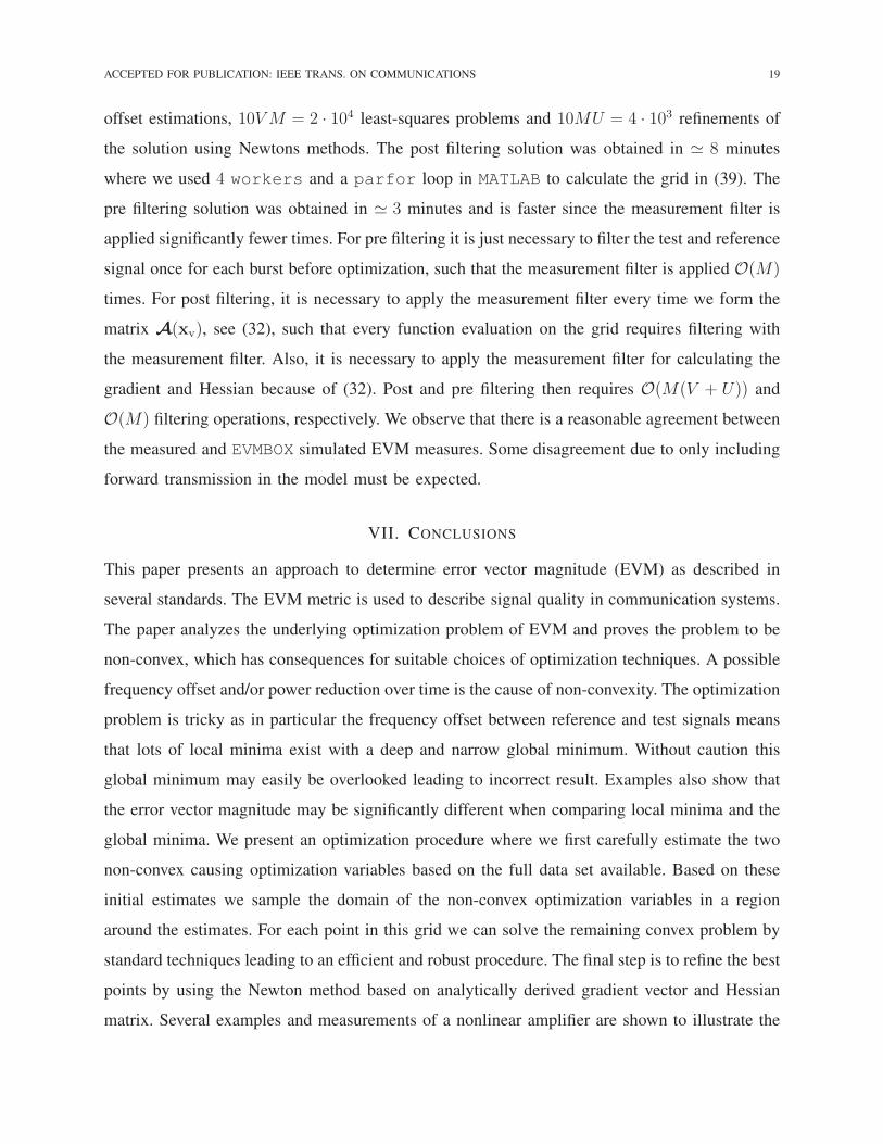
As seen from (18), the problem is to minimize the non-convex real function f(x) ≥ 0 depending

on six real optimization parameters given by x. With x3 or x4 varying we have a non-convex

optimization problem. To analyze the problem at hand, we consider a typical example of the

function f ′(xv) shown in Fig. 1. We see that x4 is very sensitive while even a change of a

factor of 30 in x3 results in almost no change in function values (the lines almost lies on top of

each other). The fluctuations also pictures why this function is not convex and warn us that any

iterative algorithm can easily get trapped in a local minima.

There are several methods, which can be applied to find a solution to the optimization problem

(36). We suggest the following approach although many variants can be developed from this1.

1) First, make initial estimations x3 for x3, and x4 for x4.

2) In a domain around the initial estimation x4, form a grid

x4 ∈ X4 =

{

x4 +2lv

V

∣

∣

∣

∣

l = ±1,±2, . . . ,±V

2

}

(39)

and evaluate the function f([x3, x4]T,x⋆

r ([x3, x4]T)) = f ′([x3, x4]

T) on this grid (we use

(38) to obtain the remaining variables). The parameters v and V determine the width and

the number of points in the grid, respectively.

3) Since we now have an estimate, which should be fairly close to the global minimum we

run an iterative algorithm on all parameters in x to find the local optimum. The iterative

algorithms are started from the U number of points with the smallest objective obtained

from step 2). With good initial conditions the local optimum may be the global optimum.

Here we rely on the less sensitive estimate of x3 and only grid x4, in which case a finer grid is

possible at the same computational cost. The use of Benders decomposition and the observation

that x3 is less sensitive, have brought the grid method from six dimensions to one dimension

which gives a reduction in computational complexity from O(V 6) to O(V ). This is an immense

reduction in computation and makes the proposed method computational feasible. Note that

since we are dealing with a non-convex problem there are no general tractable algorithm for

obtaining an optimal solution or certifying a candidate solution. Hence we have no way to

1Note that when we use the Bender decomposition strategy to obtain f ′, there are a great number of different global

optimization strategies we can follow to find a minimizer of f ′ [31]–[33].


certify the correctness of Erms in problem (6). We can only provide a an approximate solution

xp with E(xp) ≥ Erms where the inequality follows from the fact that (6) is an unconstrained

minimization problem. The signals r, t and parameters xp then form a certificate (read: proof)

of the obtained value E(xp) ≥ Erms.

One iterative algorithm which can be applied to refine a candidate solution is the Newtons

method, which gives the parameter vector for iteration i+ 1 = 1, 2, . . . , I as

x(i+1) = x(i) − λi d(i), where H(x(i))d(i) = g(x(i)) (40)

and g(x(i)) is the gradient vector containing the first-order derivatives around the point x(i), and

H(x(i)) is the Hessian matrix containing the second-order derivatives around the point x(i), and

λi is a step size. To determine the step size λi we use the Armijo rule [26]. As stopping criteria

we use the squared norm of the gradient ‖g(x(i))‖22 ≤ ǫ with ǫ = 10−3.

V. INITIAL CONDITIONS

When performing the optimization, several things can be done to speed up the process — and

help to find correct results as well. One thing is to carefully select the initial point x(0) instead

of relying on the static selection x(0) = [1, 0, 0, 0, 0, 0]T [20].

If we again consider that the problem is convex provided x3 and x4 can be treated as constants

(when optimizing for the other parameters), it is only necessary to derive initial conditions for

xv = [x3, x4] and then directly determine xr = [x1, x2, x5, x6]T by use of (38).

A. Loss factor, x3

With an estimate δ ≃ δ, we can evaluate x3(δ;n; ∆n) in (11) and use Λ(t′, δ, n) ≃ t[n]. We then

obtain an estimate x3 by averaging over all possible n and ∆n

x3 =−2

N (N + 1)

N−1∑

n=1

N−n∑

∆n=1

1

∆n

ln

{∣

∣

∣

∣

t[n]

r[n]

∣

∣

∣

∣

∣

∣

∣

∣

r[n+∆n]

t[n+∆n]

∣

∣

∣

∣

}

. (41)

B. Frequency offset, x4

We will obtain two different frequency offset estimators. A direct approach and an iterative PLL

based approach.


1) Direct approach: Lets assume that the origin offset is negligible and we aim for ex[n] = 0,

we have from (5) that

r[n] ≃ (x1 + j x2)t[n] exp[−(x3 + j κ x4) (n− 1)] . (42)

Taking the ratio r[n+∆n]/r[n] where n = 1, 2, . . . , N and ∆n = 1, 2, . . . , N − n gives

r[n+∆n]

r[n]≃

t[n+∆n]

t[n]

exp[−x3 ∆n]

exp [j κ x4 ∆n]. (43)

We need to consider that zero crossings symbols of reference or test signals (should that

unexpectedly happen) can not be used and must be omitted in (43). Now, knowing an estimate

x3 ≃ x3 we can rearrange (43), and average over the entire data set for n with ∆n = 1 to avoid

the ∆n influence on x4. This leads to the relation

A exp[j ψ] = exp [−j κ x4] (44)

where

A exp[j ψ] =exp[x3]

N − 1

N−1∑

n=1

r[n+ 1]

t[n+ 1]

t[n]

r[n], |ψ| < π . (45)

So we compute the right hand side of (45) and put this to magnitude/phase form to identify the

phase ψ. Then a method to estimate the frequency offset x4 ≃ x4 is

x4 =−ψ

κ. (46)

2) Iterative approach: Another approach is to obtain the estimate through a Phase-Locked

Loop (PLL) on the test signal where we track the instantaneous phase. Note that since we are

calculating the EVM we also have the reference signal and can hence exploit this in the PLL

design. The test signal is modelled as

t[n] =1

x1 + jx2exp

[

(x3+jκ x4)(n−1)](

r[n] + e[n] + (x5 + jx6))

. (47)

Using the estimate x3 and an instantaneous phase φ[n] we then form the following signal

gPLL[n] = t[n] exp[

− x3 · (n− 1)− jφ[n]] 1

r[n]. (48)

Note that if x3 = x3, and we aim for e[n] = 0 and (x5 + jx6) negligible, we have the signal

gPLL[n] ≃1

x1 + jx2exp

[

j(κx4 · (n− 1)− φ[n])]

. (49)


We then low-pass filter gPLL[n] to g′PLL[n] and obtain φ[n+1] = K∑n

k=1∠g′PLL[k]. In this setup

we are not interested in the synthesized frequency offset compensated signal but the frequency

offset estimation. We can then run the iterative process from n = 1, . . . , N and finally obtain

the frequency offset estimation x4 via the first-order linear least-squares regression problem

minimizeφo,x4

N∑

n=N ′

{

φo + κ x4 · (n− 1)− φ[n]}2

(50)

where φo is a constant offset representing an estimate of the steady state error. The frequency

offset estimate is then obtained as a solution to the above problem x4 = x⋆4. The parameter N ′ is a

time offset to avoid fitting in a time period where the PLL is not locked. We find experimentially

that N ′ = 15 is a reasonable choice. We also find experimentially that the iterative approach is

the most accurate approach. However, we will use the direct approach for N ≥ 5 · 104 and the

iterative approach otherwise since the direct approach is faster and as accurate for large N .

VI. NUMERICAL EXAMPLES

A toolbox named EVMBOX has been developed and is is freely distributed under the Apache

license and can be downloaded at http://www.sparsesampling.com to support the reproducible

research paradigm [27]. To support standard specific error vector magnitude (such as EDGE or

WLAN) a front-end must be made, which defines certain standard depending settings such as

a measurement filter and which parameters x1 · · · x6 that are allowed. En example for EDGE is

provided in the toolbox.

A. Validation

To validate the procedure a number of simple errors were introduced, which allows for closed

form solution of Erms. It obviously does not prove that the method is correct but it does provide

some indications for correct behavior.

Gain imbalance and phase error: Suppose the only error present is an imbalance for the

in-phase and quadrature-phase gains and we have a the following continuous time RF model

s(t) = cI rI(t) cos(ω0t) + cQ rQ(t) sin(ω0t+ φ) . (51)

Ideally, cI = cQ and φ = 0 but if this is not the case it leads to an EVM larger than zero. In

complex baseband and discrete symbol time, (51) corresponds to the test signals

ℜ{t[n]} = cI ℜ{r[n]}+ cQ sin(φ)ℑ{r[n]}, ℑ{t[n]} = cQ cos(φ)ℑ{r[n]} . (52)


Manual derivation of the optimum x1 and x2 variables (the rest are zero) leads to

x⋆1 =cI + cQ cos(φ)

c2I + c2Q, x⋆2 =

cQ sin(φ)

c2I + c2Q. (53)

Leading to an error vector magnitude as

Erms =

√

(µ− 1)2 + 4µ sin2(φ2)

2(µ2 + 1), µ =

cIcQ

. (54)

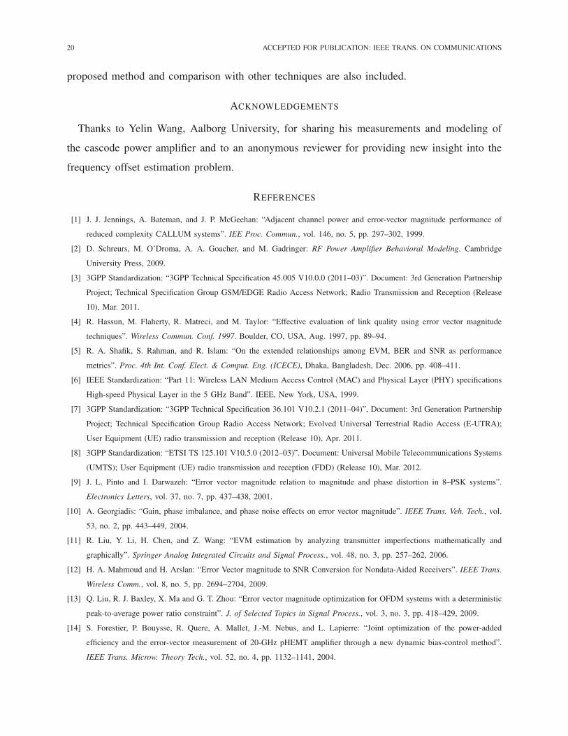
The results from applying the proposed technique and (54) are shown in Fig. 2. As observed

the agreement between the two computation techniques is excellent and as expected the model

can fully compensate for the case φ = 0, µ = 1 where we correctly observe Erms ≃ 0.

We have not found a setting of v, V from (39), which generates provable good results. We

instead rely on certain assumptions and heuristics to try ensuring that maxx4∈X4|x⋆4 − x4| is

sufficiently small. Similar interval conditions are also required in [28]. Generally we observe

that if N increases then v can be decreased because the initial estimation becomes more reliable

but we need to sample finer since the dip in f ′ becomes more narrow. However, the decrease in

v can usually compensate for the finer sampling in which case V can be kept almost constant.

In the following we assume we have a correctly identified the offset δ, such that we can

eliminate the influence from a wrongly estimated δ 6= δ and then focus on comparison and

design choices for the optimization procedures for min f(x). We generate the test signal using

t[n] =exp[(x3+jκ x4)(n−1)]

(x1 + jx2)

(

r[n] + w[n] + (x5 + jx6))

(55)

for n = 1, · · · , N where r[n] is a correlated reference signal generated with a moving average

model of order 3, MA(3) [29], using a Butterworth LP filter with cuf-off digital frequency 0.05π,

x = [x1, · · · , x6] is the true latent parameters and w = [w[1], · · · , w[N ]]T ∼ N (0, σ2I).

All timings are conducted with 4x AMD Phenom(tm) II X4 965 Processors, 3400Mhz, 16GB

RAM, MATLAB version 7.11.0.584 (R2010b) and with a single worker if nothing else is noted.

B. Comparing sampling and an iterative based method

A global optimization method for locating a minimum of a non-convex function such as f ′(xv) is

the Nelder-Mead method [30]. To test this method, we used the fminsearch implementation

of the Nelder-Mead algorithm in MATLAB with the initial conditions xv = [x3; x4] and increased

the maximum number of iterations and function evaluations to 104. We generated M = 200


reference and test signals of length N = 147. We denote xp[m] and xNM[m] the solution for

burst m of the proposed and the Nelder-Mead method, respectively. We use 4 workers and

run both the Nelder-Mead method and the sampling based method parallel across the M bursts

using the parfor loop in MATLAB. We collect the bursts with {x[m]}m=1···M = {x[m]}, where

we will use the latter notation for convenience. We also define the function C(

{x[m]})

=

|{m | E(x[m]) ≤ E(x[m])}|, that is the number of bursts the obtained EVM is better than

using the true x which generated the test signal. The reason it is possible to locate an x with

f(x) ≤ f(x), is because it is possible to slightly model the noise for finite length signals. The

result is shown in Table I, where we also use the joint EVM measure

Erms

(

{x[m]})

= 100

√

√

√

√

1

M

M∑

k=1

E2(

x[k])

(%) . (56)

Table I shows that the Nelder-Mead method is slightly slower and does not provide as accurate

results. Indeed, the Newton method is good for obtaining accurate results. The grid based method

followed by Newton optimization locates a point with a better objective in C({xp[m]}) = 200

bursts out of M = 200 compared to the EVM of the parameters that generated the test signal.

C. Comparison w.r.t. parameter sensitivity

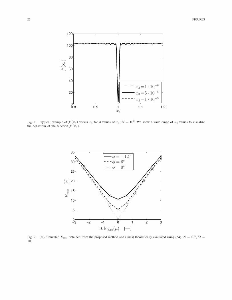
A related approach is described in [20], which uses the gradient method with independent

step size for respectively [x1; x2], [x3; x4], and [x5; x6], as well as fixed initial conditions x0 =

[1, 0, 0, 0, 0, 0]T. We compare this reference approach with the method proposed in the present

paper. The difficult part of the optimization problem seems to be estimation of the parameter x4.

To exemplify this we set the true x = [1, −0.5, 6.53 · 10−4, x4, 0, 0]T, N = 250 and investigate

the obtained Erms values for different x4. The result is presented in Fig. 3. We see that the

reference gradient method with independent step sizes achieves the same Erms value for some

0 ≤ x4 ≤ 0.4. But for x4 ≥ 0.5 and x4 ≤ −0.1, the gradient method with fixed initial conditions

gets trapped in a local minima with high Erms (since the proposed method finds an estimate

with significantly lower EVM). We used I = 105 iterations for the reference gradient method to

ensure full convergence.


D. Comparison w.r.t. accuracy and efficiency

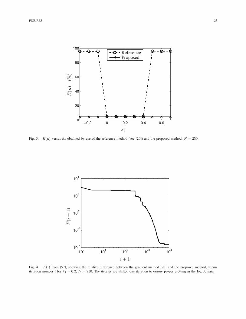
Continuing with the same example as in VI-C, we now fix x4 = 0.2, and analyse the objective

versus iteration number. We investigate the relative difference between the objective from the

algorithm in [20] at iteration i using the gradient approach and the solution found by the proposed

method given by

F (i) =f(x

(i)g )− f(xp)

f(xp)(57)

where x(i)g is the x-vector for iteration i generated by the gradient based reference method

[20], and f(xp) is the objective of the solution provided by the proposed method. The result is

shown in Fig. 4, which indicates that the gradient method with fixed initial conditions requires

approximately 3200 iterations to obtain an iterate within 1% accuracy of the proposed method.

In our implementation, 3200 iterations of the reference method requires 2.4 s while the proposed

method found a solution in 0.07 s. We see that the gradient based reference method has trouble

finding a solution within an accuracy of 0.1%, and never obtains an iterate with a lower objective

than that of the proposed method since the relative difference is positive. Note that the solution xp

provided by the proposed method is not necessarily the solution x⋆ to the optimization problem.

But we do have f(xp) < f(x) meaning that not even knowing the true x-vector, which generated

the test data, yields a lower objective than the proposed method.

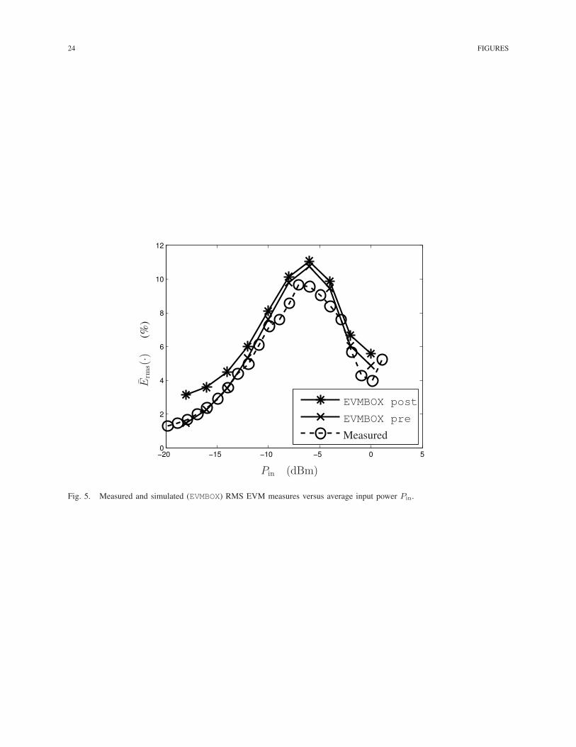
E. EDGE

Using a cascode power amplifier, a nonlinear AM-AM/AM-PM model was developed for this

device using PNA-X measurements [34]. Only the forward S21 transmission parameter was

included in the model for simplicity (input reflection was below −10 dB). The response to an

EDGE input signal was then computed based on a cubic spline interpolation of the AM-AM/AM-

PM model data. It was verified that the signal was in-bound of the model. The EDGE standard

calls for post filtering [3], but we also calculate the pre filtering case for comparison. The

EDGE standard requirement was implemented: 1) compensation using all parameters x1 · · · x6

is allowed 2) the required measurement filter and 3) the linear function t[n] = Λ(t′, δ, n) =

t′[(n−1)Θ+δ+1]. The reference and test signals were then passed to EVMBOX, which computed

the 10 EVM points for different Pin across M = 200 burst using V = 10 grid points and

refines U = 2 grid points using Newtons method. This gives in total 10M = 2 · 103 time


offset estimations, 10VM = 2 · 104 least-squares problems and 10MU = 4 · 103 refinements of

the solution using Newtons methods. The post filtering solution was obtained in ≃ 8 minutes

where we used 4 workers and a parfor loop in MATLAB to calculate the grid in (39). The

pre filtering solution was obtained in ≃ 3 minutes and is faster since the measurement filter is

applied significantly fewer times. For pre filtering it is just necessary to filter the test and reference

signal once for each burst before optimization, such that the measurement filter is applied O(M)

times. For post filtering, it is necessary to apply the measurement filter every time we form the

matrix A(xv), see (32), such that every function evaluation on the grid requires filtering with

the measurement filter. Also, it is necessary to apply the measurement filter for calculating the

gradient and Hessian because of (32). Post and pre filtering then requires O(M(V + U)) and

O(M) filtering operations, respectively. We observe that there is a reasonable agreement between

the measured and EVMBOX simulated EVM measures. Some disagreement due to only including

forward transmission in the model must be expected.

VII. CONCLUSIONS

This paper presents an approach to determine error vector magnitude (EVM) as described in

several standards. The EVM metric is used to describe signal quality in communication systems.

The paper analyzes the underlying optimization problem of EVM and proves the problem to be

non-convex, which has consequences for suitable choices of optimization techniques. A possible

frequency offset and/or power reduction over time is the cause of non-convexity. The optimization

problem is tricky as in particular the frequency offset between reference and test signals means

that lots of local minima exist with a deep and narrow global minimum. Without caution this

global minimum may easily be overlooked leading to incorrect result. Examples also show that

the error vector magnitude may be significantly different when comparing local minima and the

global minima. We present an optimization procedure where we first carefully estimate the two

non-convex causing optimization variables based on the full data set available. Based on these

initial estimates we sample the domain of the non-convex optimization variables in a region

around the estimates. For each point in this grid we can solve the remaining convex problem by

standard techniques leading to an efficient and robust procedure. The final step is to refine the best

points by using the Newton method based on analytically derived gradient vector and Hessian

matrix. Several examples and measurements of a nonlinear amplifier are shown to illustrate the


proposed method and comparison with other techniques are also included.

ACKNOWLEDGEMENTS

Thanks to Yelin Wang, Aalborg University, for sharing his measurements and modeling of

the cascode power amplifier and to an anonymous reviewer for providing new insight into the

frequency offset estimation problem.

REFERENCES

[1] J. J. Jennings, A. Bateman, and J. P. McGeehan: “Adjacent channel power and error-vector magnitude performance of

reduced complexity CALLUM systems”. IEE Proc. Commun., vol. 146, no. 5, pp. 297–302, 1999.

[2] D. Schreurs, M. O’Droma, A. A. Goacher, and M. Gadringer: RF Power Amplifier Behavioral Modeling. Cambridge

University Press, 2009.

[3] 3GPP Standardization: “3GPP Technical Specification 45.005 V10.0.0 (2011–03)”. Document: 3rd Generation Partnership

Project; Technical Specification Group GSM/EDGE Radio Access Network; Radio Transmission and Reception (Release

10), Mar. 2011.

[4] R. Hassun, M. Flaherty, R. Matreci, and M. Taylor: “Effective evaluation of link quality using error vector magnitude

techniques”. Wireless Commun. Conf. 1997. Boulder, CO, USA, Aug. 1997, pp. 89–94.

[5] R. A. Shafik, S. Rahman, and R. Islam: “On the extended relationships among EVM, BER and SNR as performance

metrics”. Proc. 4th Int. Conf. Elect. & Comput. Eng. (ICECE), Dhaka, Bangladesh, Dec. 2006, pp. 408–411.

[6] IEEE Standardization: “Part 11: Wireless LAN Medium Access Control (MAC) and Physical Layer (PHY) specifications

High-speed Physical Layer in the 5 GHz Band”. IEEE, New York, USA, 1999.

[7] 3GPP Standardization: “3GPP Technical Specification 36.101 V10.2.1 (2011–04)”, Document: 3rd Generation Partnership

Project; Technical Specification Group Radio Access Network; Evolved Universal Terrestrial Radio Access (E-UTRA);

User Equipment (UE) radio transmission and reception (Release 10), Apr. 2011.

[8] 3GPP Standardization: “ETSI TS 125.101 V10.5.0 (2012–03)”. Document: Universal Mobile Telecommunications Systems

(UMTS); User Equipment (UE) radio transmission and reception (FDD) (Release 10), Mar. 2012.

[9] J. L. Pinto and I. Darwazeh: “Error vector magnitude relation to magnitude and phase distortion in 8–PSK systems”.

Electronics Letters, vol. 37, no. 7, pp. 437–438, 2001.

[10] A. Georgiadis: “Gain, phase imbalance, and phase noise effects on error vector magnitude”. IEEE Trans. Veh. Tech., vol.

53, no. 2, pp. 443–449, 2004.

[11] R. Liu, Y. Li, H. Chen, and Z. Wang: “EVM estimation by analyzing transmitter imperfections mathematically and

graphically”. Springer Analog Integrated Circuits and Signal Process., vol. 48, no. 3, pp. 257–262, 2006.

[12] H. A. Mahmoud and H. Arslan: “Error Vector magnitude to SNR Conversion for Nondata-Aided Receivers”. IEEE Trans.

Wireless Comm., vol. 8, no. 5, pp. 2694–2704, 2009.

[13] Q. Liu, R. J. Baxley, X. Ma and G. T. Zhou: “Error vector magnitude optimization for OFDM systems with a deterministic

peak-to-average power ratio constraint”. J. of Selected Topics in Signal Process., vol. 3, no. 3, pp. 418–429, 2009.

[14] S. Forestier, P. Bouysse, R. Quere, A. Mallet, J.-M. Nebus, and L. Lapierre: “Joint optimization of the power-added

efficiency and the error-vector measurement of 20-GHz pHEMT amplifier through a new dynamic bias-control method”.

IEEE Trans. Microw. Theory Tech., vol. 52, no. 4, pp. 1132–1141, 2004.


[15] M. D. McKinley, K. A. Remley, M. Myslinski, J. S. Kenney, D. Schreurs, and B. Nauwelaers. “EVM calculation for

broadband modulated signals”. 64th ARFTG Microwave Measurements Conf. Dig.. Orlando, FL, USA. Dec. 2004, pp.

45-52.

[16] H. Ku and J. S. Kenney: “Estimation of error vector magnitude using two-tone intermodulation distortion measurements”.

IEEE Microwave Theory and Tech. Symp. Dig., vol. 3, Phoenix, AZ, USA, May 2001, pp. 17–20.

[17] S. Freisleben: “Semi-analytical computation of error vector magnitude for UMTS SAW filters”. Proc. IEEE Ultrasonics

Symp. 2002, vol. 1, 2002, pp. 109–112.

[18] S. Yamanouch, K. Kunihiro, and H. Hida: “An efficient algorithm for simulating error vector magnitude in nonlinear

OFDM amplifiers”. Proc. IEEE Custom Integrated Circuits Conf., Orlando, FL, USA, Oct. 2004, pp. 129–132.

[19] E. Acar, S. Ozev, and K. B. Redmond: “Enhanced error vector magnitude (EVM) measurements for testing WLAN

transceivers”. Proc. 2006 IEEE/ACM Int. Conf. Computer-Aided Design, San Jose, CA, USA, Nov. 2006, pp. 210–216.

[20] A. Mashhour, and A. Borjak: “A method for computing error vector magnitude in GSM EDGE systems – Simulation

results”. IEEE Commun. Letters, vol. 5, no. 3, pp. 88–91, 2001.

[21] S. Xia, H. Chen, Z. Xu, and C. Hong: “Key algorithms for accurate GSM EDGE EVM measurement on ATE platform”.

8th Int. Conf. Solid-State and Integrated Circuit Tech., Shanghai, China, Oct. 2006, pp. 2151–2154.

[22] M. C. Jeruchim, P. Balaban, and K. S. Shanmugam: Simulation of Communication Systems: Modeling, Methodology, and

Techniques. Second edition. Kluwer, 2000.

[23] S. Boyd and L. Vandenberghe. Convex Optimization. Cambridge University Press, 2004.

[24] J. F. Benders: “Partitioning procedures for solving mixed-variables programming problems”. Numerische Mathematik, vol.

4, pp. 238–252, 1962.

[25] A. M. Geoffrion: “Generalized Benders decomposition”. J. of Optimization Theory and Applicat., vol. 10, no. 4, pp.

237–260, 1972.

[26] D. P. Bertsekas: Nonlinear Programming. Athena Scientific. Belmont, MA, USA, 1995.

[27] P. Vandewalle, J. Kovacevic, and M. Vetterli “Reproducible research in signal processing [What, why, and how]”. IEEE

Signal Process. Mag., vol. 26, no. 3, pp. 37–47, May 2009.

[28] E. Hansen and G. W. Walster: Global Optimization Using Interval Analysis – Second Edition, Revised and Expanded,

CRC Press, 2003.

[29] S. Haykin: Adaptive Filter Theory. 4th Ed., Prentice Hall, Upper Saddle River, NJ, USA, 2002.

[30] J. A. Nelder and R. Mead: “A simplex method for function minimization”. The Computer J., vol. 7, no. 4, pp. 308–313,

1965.

[31] A. Torn and A. Zilinskas, Global Optimization, Lecture Notes in Computer Science, Vol. 350, 1989.

[32] R. Host, P. M. Pardalos, and N. V. Thoai, Introduction to Global Optimization, 2nd Edition, Kluwer Academic Publishers,

2000.

[33] Ed. P. M. Pardalos and H. E. Romeijn, Handbook of Global Optimization, Vol. 2, Kluwer Academic Press, 2002.

[34] Y. Wang, D. Sira, T. S. Nielsen, O. K. Jensen and T. Larsen, “On wafer X-parameter based modeling of a switching

cascode power amplifier”, IEEE 29th Norchip Conf., Lund, Sweden, Nov. 2011, pp. 1-4.

22 FIGURES

0.8 0.9 1 1.1 1.20

20

40

60

80

100

120

x4

f′ (xv)

x3=1 · 10−6

x3=5 · 10−5

x3=1 · 10−3

Fig. 1. Typical example of f ′(xv) versus x4 for 3 values of x3. N = 103. We show a wide range of x4 values to visualize

the behaviour of the function f ′(xv).

−3 −2 −1 0 1 2 30

5

10

15

20

25

30

35

Erm

s[%

]

φ = −12◦

φ = 0◦φ = 6◦

10 log10(µ) [—]

Fig. 2. (×) Simulated Erms obtained from the proposed method and (lines) theoretically evaluated using (54). N = 105,M =10.

FIGURES 23

−0.2 0 0.2 0.4 0.60

20

40

60

80

100

E(x)

(%)

x4

ReferenceProposed

Fig. 3. E(x) versus x4 obtained by use of the reference method (see [20]) and the proposed method. N = 250.

100

101

102

103

104

10−4

10−2

100

102

104

F(i+1)

i+ 1

Fig. 4. F (i) from (57), showing the relative difference between the gradient method [20] and the proposed method, versus

iteration number i for x4 = 0.2, N = 250. The iterates are shifted one iteration to ensure proper plotting in the log domain.

24 FIGURES

−20 −15 −10 −5 0 50

2

4

6

8

10

12

EVMBOX pre

EVMBOX post

Measured

Erm

s(·)

(%)

Pin (dBm)

Fig. 5. Measured and simulated (EVMBOX) RMS EVM measures versus average input power Pin.


— Time [s] Erms

(

{x[m]})

C(

{x[m]})

Sampled xp[m] 2.26 8.75 200

Nelder-Mead xNM[m] 4.47 8.84 194

TABLE I

EXECUTION TIME, JOINT EVM, AND COMPARISON MEASURE FOR THE PROPOSED SAMPLED AND THE NELDER-MEAD

METHOD. THE GENERATED DATA GIVES Erms({x[m]}) = 8.88.

Aalborg Universitet Robust Computation of Error Vector ...

Documents

Transcript of Aalborg Universitet Robust Computation of Error Vector ...