AA 2009-2010 Facoltà di Scienze MM, FF e NN … · – Model-based, region-based • Filtering ......

Image Processing for Bioinformatics

AA 2009-2010

Facoltà di Scienze MM, FF e NN

Dipartimento di Informatica

Università di Verona

General information

• Teacher: Gloria Menegaz

• Assistant: Francesca Pizzorni

• Scheduling– Theory

• Mon. 14.30 to 16.30• Wed. 10.30 to 11.30

– Laboratory• Wed. 11.30 to 13.30

– Tutoring (ricevimento)• by appointment (email)

– Start and end dates• March 1°, 2010 – Mid May 2010

• Exam– TBD

• Support– Slides of the course– Books

Contents

Classical IP

• Review of Fourier Transform

• Extension to 2D

• Sampling in 2D

• Quantization

• Edge detection– Model-based, region-based

• Filtering – denoising, deblurring, image

enhancement

• Segmentation techniques

• Basics of pattern recognition– Clustering, classification

Advanced Topics

• Color imaging

• Introduction to stochastic processes

• Microarray image analysis

Why do we process images?

• To facilitate their storage and transmission

• To prepare them for display or printing

• To enhance or restore them

• To extract information from them

• To hide information in them

Image types

Optical (CCD)radar (SAR)

underwater infrared medical (MRI)

Microarray images

Image Processing Example

• Image Restoration

Original image Blurred Restored by Wiener filter


• Noise Removal

Noisy image Denoised by Median filter


• Image Enhancement

Histogram equalization

Image Processing Example• Artifact Reduction in Digital Cameras

Original scene Captured by a digital camera Processed to reduce artifacts


• Image Compression

Original image 64 KB

JPEG compressed 15 KB

JPEG compressed 9 KB


• Object Segmentation

“Rice” image Edges detected using Canny filter


• Resolution Enhancement


• Watermarking

Original image

Hidden message

Generate watermark

Watermarked image

Secret key


• Face Recognition

Surveillance video

Search in the database

Image Processing Example• Fingerprint Matching

Image Processing Example• Segmentation

Image Processing Example• Texture Analysis and Synthesis

Pattern repeated Computer generated

Photo


• Face detection and tracking

http://vasc.ri.cmu.edu/NNFaceDetector/

Image Processing Example• Face Tracking

Image Processing Example• Object Tracking

Image Processing Example• Visually Guided Surgery

Taxonomy of the IP domain

Computer vision

Computer graphicsPattern recognition

Image processing

Computer graphics

• Algorithms allowing to generate artificial images and scenes

• Model-based• Scenes are created based on models

• Visualization often rests on 2D projections

• Hot topic: generate perceptually credible scenes– Image-based modeling & rendering

DNA VIRUS - Herpes

HEARTH (interior) BRAIN (visual cortex)

Computer vision

• Methods for estimating the geometrical and dynamical properties of the imaged scene based on the acquired images– Scene description based on image features

• Complementary to computer graphics– Get information about the 3D real world based on its 2D projections in

order to automatically perform predefined tasks

Pattern Recognition

• Image interpretation

• Identification of basic and/or complex structures– implies pre-processing to reduce the intrinsic redundancy in the input

data– knowledge-based

• use of a-priori knowledge on the real world• stochastic inference to compensate for partial data

• Key to clustering and classification

• Applications– medical image analysis– microarray analysis– multimedia applications

Pattern Recognition

• Clustering– data analysis aiming at constructing and characterizing clusters (sets)– analisi dei dati per trovare inter-relazioni e discriminarli in gruppi (senza

conoscenza a priori)

• Feature extraction and selection– reduction of data dimensionality

• Classification– Structural (based on a predefined “syntax”):

• each pattern is considered as a set of primitives• clustering in the form of parsing

– Stochastic• Based on statistics (region-based descriptors)

Applications

• Efficiently manage different types of images– Satellite, radar, optical..– Medical (MRI, CT, US), microarrays

• Image representation and modeling

• Quality enhancement– Image restoration, denoising

• Image analysis– Feature extraction and exploitation

• Image reconstruction from projections– scene reconstruction, CT, MRI

• Compression and coding

Typical issues

Multimedia

• Image resampling and interpolation

• Visualization and rendering

• Multispectral imaging– Satellite, color

• Motion detection, tracking

• Automatic quality assessment

• Data mining– query by example

Medical imaging

• Image analysis– optical devices, MRI, CT, PET, US

(2D to 4D)

• Image modeling– Analysis of hearth motion, models

of tumor growth, computer assisted surgery

• Telemedicine– remote diagnosis, distributed

systems, medical databases

Other applications

• Quality control

• Reverse engineering

• Surveillance (monitoring and detection of potentially dangerous situations)

• Social computing (face and gesture recognition for biometrics and behavioural analysis)

• Robotics (machine vision)

• Virtual reality

• Telepresence

Query by example

Segmentation

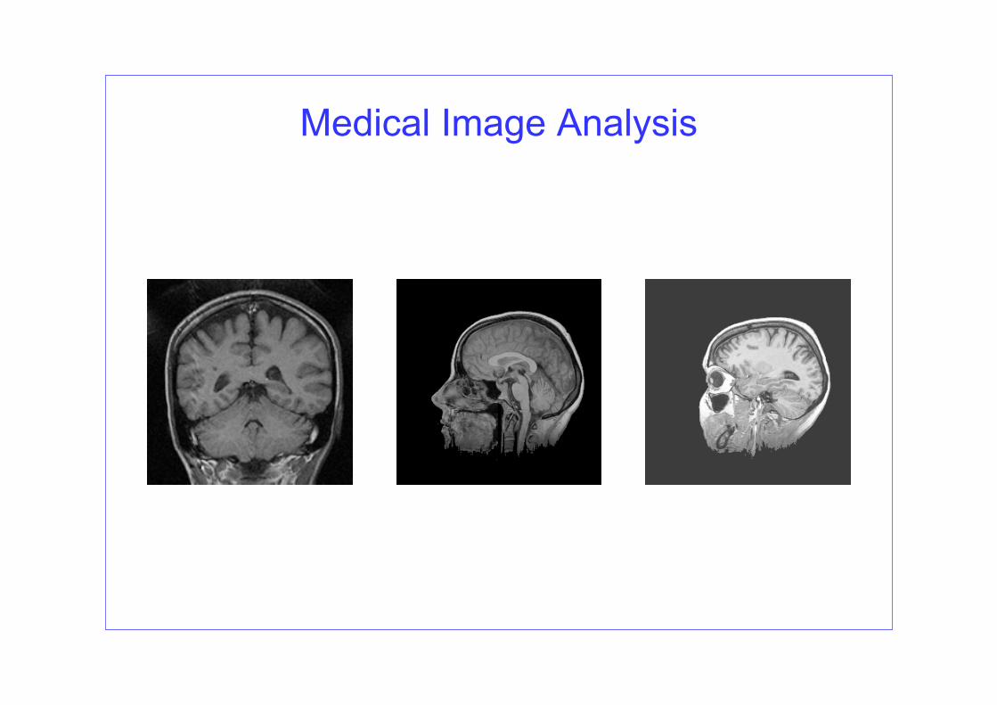
Medical Image Analysis

Sequence analysis

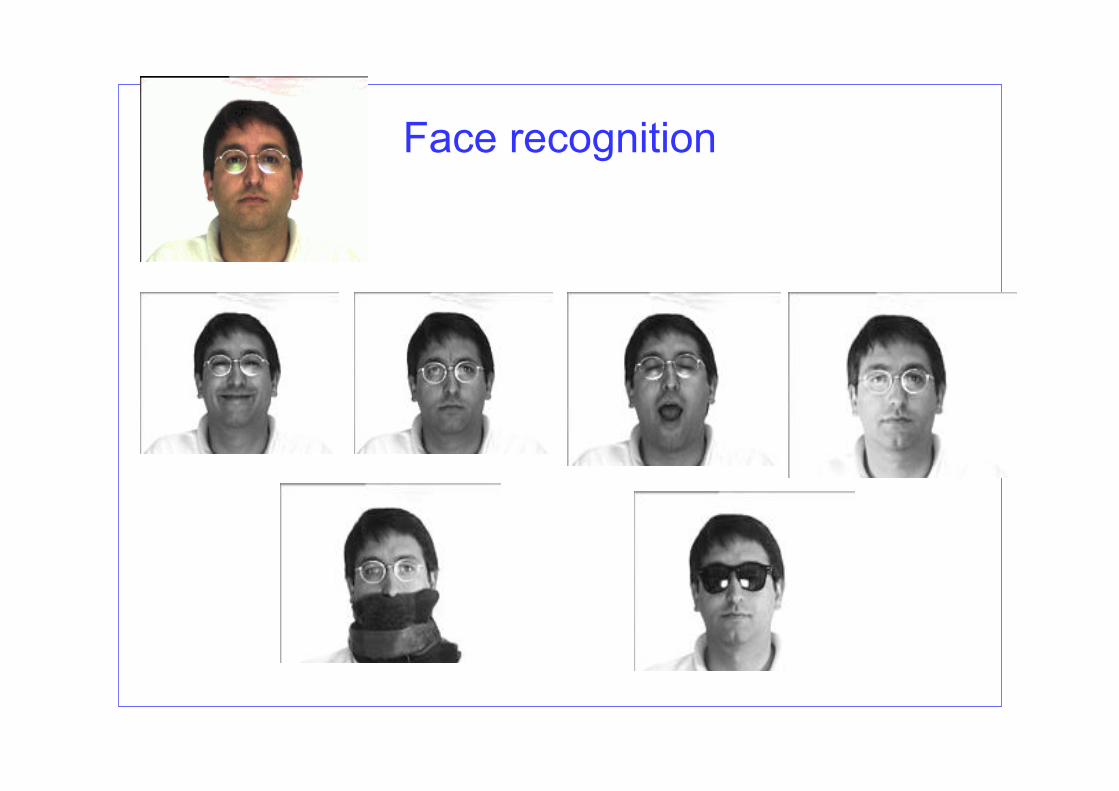
Face recognition

Coppia di immagini stereo (immagini ottiche)

Immagine di disparità: i punti più chiari rappresentano oggetti più vicini all’osservatore

Stereo pairs

Texture analysis

Medical textures

MI applications

• Tumor identitication and staging

MI applications

• Exploring brain anatomy by diffusion weighted MRI

Compression and coding

H encoded data

Object-based processing

Mosaicing

Low level

High level

Rawimage data

Preprocessing

TransformsSegmentationEdge detection

Feature extraction FeatureObjects

SpectrumSegmentsEdge/lines

NeighbourhoodSubimage

Pixel

Operations Low-level image representationHierarchical Image Pyramid

Image formation and fundamentals

IP frameworkNatural scene

Digital image

15 25 44 100

Image Processing

System

filteringtransformscoding....

Image rendering

capturesamplingquantizationcolor space

Is this good quality

How can I protect my data?

What is the best I can get over

my phone line?

How much will it cost?

NetworkNetwork

IP: basic steps

{15,1,2} {25,44,1}….

A/D conversion

Sampling (2D) Quantization

Analog image

Digital image

(capturing device)

Digital Image AcquisitionSensor array

• When photons strike, electron-hole pairs are generated on sensor sites.

• Electrons generated are collected over a certain period of time.

• The number of electrons are converted to pixel values. (Pixel is short for picture element.)

Object(surface element)

Surface reflectance

Optical axis

Light source

N

CAMERA

Sensors

theta

Image capture

VM1

VM1 - radianza: energia che viene emessa dall'elemento di superficie- irradianza: energia che colpisce la camera e dipende da lo spettro della luce, la riflettanza della superficie (che cambia lo spettro) e la sensibilità spettrale del sensoreswan; 14/01/2004

Digital Image Acquisition

Two types of discretization:1. There are finite number of

pixels. (sampling → Spatial resolution)

2. The amplitude of pixel is represented by a finite number of bits. (Quantization → Gray-scale resolution)


Take a look at this cross section


• 256x256 - Found on very cheap cameras, this resolution is so low that the picture quality is almost always unacceptable. This is 65,000 total pixels.

• 640x480 - This is the low end on most "real" cameras. This resolution is ideal for e-mailing pictures or posting pictures on a Web site.

• 1216x912 - This is a "megapixel" image size -- 1,109,000 total pixels -- good for printing pictures.

• 1600x1200 - With almost 2 million total pixels, this is "high resolution." You can print a 4x5 inch print taken at this resolution with the same quality that you would get from a photo lab.

• 2240x1680 - Found on 4 megapixelcameras -- the current standard -- this allows even larger printed photos, with good quality for prints up to 16x20 inches.

• 4064x2704 - A top-of-the-line digital camera with 11.1 megapixels takes pictures at this resolution. At this setting, you can create 13.5x9 inch prints with no loss of picture quality.

Basics: greylevel images

10020001005010020010020050050

90200100100

Images : Matrices of numbersImage processing : Operations among numbersbit depth : number of bits/pixelN bit/pixel : 2N-1 shades of gray (typically N=8)

Matrix Representation of Images

• A digital image can be written as a matrix

1 2

[0,0] [0,1] [0, 1][1,0] [1,1] [1, 1]

[ , ]

[ 1,0] [ 1, 1] MxN

x x x Nx x x N

x n n

x M x M N

−⎡ ⎤⎢ ⎥−⎢ ⎥=⎢ ⎥⎢ ⎥− − −⎣ ⎦

35 45 2043 64 5210 29 39

⎡ ⎤⎢ ⎥⎢ ⎥⎢ ⎥⎣ ⎦

Digital images acquisition

• Analog camera+A/D converter

• Digital cameras– CCDs (Charge Coupled Devices)– CMOS technology

• In both cases: optics– lenses, diaphragms

Matrices of photo sensors collecting photons of given wavelength

Features of the capture devices:

• Size and number of photo sites• Noise• Transfer function of the optical filter

Color images

• Each colored pixel corresponds to a vector of three values {C1,C2,C3}

• The characteristics of the components depend on the chosen colorspace(RGB, YUV, CIELab,..)

C1 C2 C3

Digital Color Images

• 1 2[ , ]Rx n n1 2[ , ]Gx n n1 2[ , ]Bx n n

Color channels

Red Green Blue

The physical perspective

The perceptual perspective

Simultaneous contrast

Color

• Chromatic induction

Color

• Human vision– Color encoding (receptor level)– Color perception (post-receptoral

level)– Color semantics (cognitive level)

• Colorimetry– Spectral properties of radiation– Physical properties of materials

Color vision(Seeing colors)

Colorimetry(Measuring colors)

Color categorization and naming

(understanding colors)

MODELS

Bayer matrix

Typical sensor topology in CCD devices. The green is twice as numerous as red and blue.

Displays

LCD

CRT

Color imaging

• Color reproduction– Printing, rendering

• Digital photography– High dynamic range images– Mosaicking– Compensation for differences in illuminant (CAT: chromatic adaptation

transforms)

• Post-processing– Image enhancement

• Coding– Quantization based on color CFSs (contrast sensitivity function)– Downsampling of chromatic channels with respect to luminance

Some definitions

• Digital images– Sampling+quantization

• Sampling– Determines the graylevel value of each pixel

• Pixel = picture element

• Quantization– Reduces the resolution in the graylevel value to that set by the

machine precision

• Images are stored as matrices of unsigned chars

Resolution

• Sensor resolution (CCD): Dots Per Inch (DPI)– Number of individual dots that can be placed within the span of one

linear inch (2.54 cm)

• Image resolution– Pixel resolution: NxM– Spatial resolution: Pixels Per Inch (PPI)– Spectral resolution: bandwidth of each spectral component of the image

• Color images: 3 components (R,G,B channels)• Multispectral images: many components (ex. SAR images)

– Radiometric resolution: Bits Per Pixel (bpp)• Greylevel images: 8, 12, 16 bpp• Color images: 24bpp (8 bpp/channel)

– Temporal resolution: for movies, number of frames/sec• Typically 25 Hz (=25 frames/sec)

VM2

VM2 da book Shapiroswan; 10/04/2003

Example: pixel resolution

Image ResolutionDon’t confuse image size and resolution.

Bit Depth – Grayscale Resolution

8 bits

7 bits

6 bits 5 bits

Bit Depth – Grayscale Resolution4 bits

3 bits

2 bits 1 bit

File format

• Many image formats (about 44)

• BMP, lossless

• TIFF, lossless/lossy

• GIF (Graphics Interchange Format)– Lossless, 256 colors, copyright protected

• JPEG (Joint Photographic Expert Group)– Lossless and lossy compression– 8 bits per color (red, green, blue) for a 24-bit total

• PNG (Portable Network Graphics)– Freewere– supports truecolor (16 million colours)

AA 2009-2010 Facoltà di Scienze MM, FF e NN … · – Model-based, region-based • Filtering ......

Documents

Transcript of AA 2009-2010 Facoltà di Scienze MM, FF e NN … · – Model-based, region-based • Filtering ......