a workshop in scanning probe microscopy -...
147
Nanoscience on the tip a workshop in scanning probe microscopy NANOTECHNOLOGY UNDERGRADUATE EDUCATION: USING NANOSCIENCE INSTRUMENTATION FOR QUALITY UNDERGRADUATE EDUCATION 1 μm Seattle, Washington July 6 – 10, 2009
Transcript of a workshop in scanning probe microscopy -...

Nanoscience on the tipa workshop in scanning probe microscopy
NANOTECHNOLOGY UNDERGRADUATE
EDUCATION:
USING NANOSCIENCE INSTRUMENTATION
FOR QUALITY UNDERGRADUATE
EDUCATION
1 µmSeattle, Washington
July 6 – 10, 2009

2009Laboratory Course 1
Nanoscience on the tip a workshop in scanning probe microscopy
T A B L E O F C O N T E N T S
Scope................................................................................................................................... 3
Motivation, Objective and Preface................................................................................................ 3 Organization of the 2009 SPM Workshop......................................................................... 4
Format – Daily Schedule............................................................................................................... 4 Local Maps .................................................................................................................................... 5
Workshop Contacts............................................................................................................ 7 NUE UNIQUE Partners and Sponsors............................................................................... 7 Biographical Sketches ....................................................................................................... 8 Acknowledgment ............................................................................................................... 9 Workshop 2009 Participants............................................................................................ 10
2009Laboratory Course 2
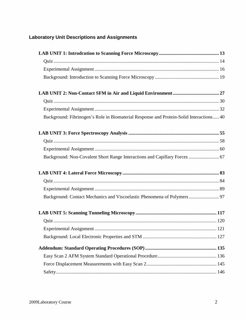
Laboratory Unit Descriptions and Assignments
LAB UNIT 1: Introdcution to Scanning Force Microscopy.................................................. 13 Quiz ......................................................................................................................................... 14
Experimental Assignment ....................................................................................................... 16
Background: Introduction to Scanning Force Microscopy ..................................................... 19
LAB UNIT 2: Non-Contact SFM in Air and Liquid Environment ...................................... 27 Quiz ......................................................................................................................................... 30
Experimental Assignment ....................................................................................................... 32
Background: Fibrinogen’s Role in Biomaterial Response and Protein-Solid Interactions..... 40
LAB UNIT 3: Force Spectroscopy Analysis ........................................................................... 55 Quiz ......................................................................................................................................... 58
Experimental Assignment ....................................................................................................... 60
Background: Non-Covalent Short Range Interactions and Capillary Forces ......................... 67
LAB UNIT 4: Lateral Force Microscopy................................................................................ 83 Quiz ......................................................................................................................................... 84
Experimental Assignment ....................................................................................................... 89
Background: Contact Mechanics and Viscoelastic Phenomena of Polymers ......................... 97
LAB UNIT 5: Scanning Tunneling Microscopy ................................................................... 117 Quiz ....................................................................................................................................... 120
Experimental Assignment ..................................................................................................... 121
Background: Local Electronic Properties and STM ............................................................. 127
Addendum: Standard Operating Procedures (SOP) ........................................................... 135 Easy Scan 2 AFM System Standard Operational Procedure................................................. 136
Force Displacement Measurements with Easy Scan 2.......................................................... 145
Safety..................................................................................................................................... 146

2009Laboratory Course 3 3
S C O P E
Motivation Since the invention of the scanning tunneling microscope (STM) in 1981 by Gerd Binnig and Heinrich Rohrer (Nobel Prize in Physics 1986), scanning probe microscopy (SPM) techniques have dazzled scientist and engineers in nearly every field from natural sciences to liberal arts, and nucleated the new discipline of Nanoscience and Nanotechnology. The birth of such a highly interdisciplinary field is an attest to the changing times in a world that moves from educating specialists to generalists. The true power of SPM techniques, which assisted in removing boundaries between disciplines, lays in its simplicity to provide access to the nanoworld in terms of visualization and manipulation. Hence, it is only perceivable that SPM offers an outstanding educational tool for schools. Objective The overarching objective of the NUE UNIQUE Program is to develop a nationally replicable model of a sustainable and up-to-date undergraduate teaching laboratory of scanning probe methods applied to nanosciences and nanotechnology. To this end, a partnership between researchers and educators at the University of Washington (UW) and the North Seattle Community College (NSCC), and two companies - Nanosurf, AG (Liestal, Switzerland) and nanoscience Instruments (Phoenix, AZ) has been forged within this partnership a new paradigm of initiating, operating and maintaining a SPM laboratory will be developed and tested that provides a truly hands-on experience in a classroom laboratory setting for a small number of students per instrument involving a variety of SPM techniques and nanoscience/engineering topics. Preface Like the first and second, this third workshop organized within the boundaries of this paradigm of initiating, operating and maintaining a SPM laboratory serves a class of 16 undergraduate students of diverse academic background with a one-week hands-on experience in small groups of 4 students per instrument. The students gain experience in a variety of different areas from protein adsorption kinetics, contact mechanics, polymer relaxation, Van der Waals and capillary forces to quantum mechanical properties.
NUE UNIQUE
René M. Overney Director

2009Laboratory Course 4
O r g a n i z a t i o n o f t h e 2 0 0 9 S P M W o r k s h o p
Format – Daily Schedule
Monday Tuesday Wednesday Thursday Friday July 6 July 7 July 8 July 9 July 10
9:00 a.m. Welcome
Profs Overney, Sarikaya
Milnor-Roberts Room
8:45 – 9:30 a.m. Individual Group Lecture by TA on
Lab Unit Topic Location as per Table 1 below
8:45 – 9:30 a.m. Individual Group Lecture by TA on
Lab Unit Topic Location as per Table 1 below
8:45 – 9:30 a.m. Individual Group Lecture by TA on
Lab Unit Topic Location as per Table 1 below
8:00 – 8:45 a.m. Individual Group Lecture by TA on
Lab Unit Topic Location as per Table 1 below
9:15 – 10.00 a.m. Lecture:
Introduction to SPM
Prof Overney Milnor-Roberts Room
9:30 – 5:00 p.m.
Work on Lab Units in Assigned
Groups (see Group
Assignment Sheet)
9:30 – 5:00 p.m.
Work on Lab Units in Assigned
Groups (see Group
Assignment Sheet)
9:30 – 5:00 p.m.
Work on Lab Units in Assigned
Groups (see Group
Assignment Sheet)
8:45 – 2:30 p.m.
Work on Lab Units in Assigned
Groups (see Group
Assignment Sheet) 10:15 – 11.00 a.m. Lecture: Interaction
Forces, and Contact Mechanics
Prof Overney Milnor-Roberts Room Wilcox Hall (2nd Floor) 11:15 – 11:45 a.m.
GEMSEC and Biomimetics Prof Sarikaya
Milnor-Roberts Room Wilcox Hall (2nd Floor)
Lunch in Assigned Groups
1:00 p.m. Laboratory Lab Unit 1 AFM - NC
First Hands-On Atomic Force
Microscopy (AFM) Wilcox 233 and 235
Table 1: Lab Unit Location and Group Schedule Tuesday Wednesday Thursday Friday
Lab Unit 2 AFM-Bio
Roberts 121 Chris So
Group 1 Group 4 Group 3 Group 2
Lab Unit 3 AFM-Forces
Wilcox 235 Dmitriy
Khatayevich
Group 2 Group 1 Group 4 Group 3
Lab Unit 4 LFM
Benson 319 Dan Knorr
Group 3 Group 2 Group 1 Group 4
Lab Unit 5 STM
Wilcox 233 Lakshmi
Kocherlakota
Group 4 Group 3 Group 2 Group 1
“Homework”: Involves reading of the background information of the day and answering the theoretical questions. Due before the lecture next day.
Friday 2:30 – p.m. Final Remarks
Certificates Profs Overney, Sarikaya
Milnor-Roberts Room Wilcox Hall (2nd Floor)
3:30 p.m. Adjourned
2009Laboratory Course 5 5
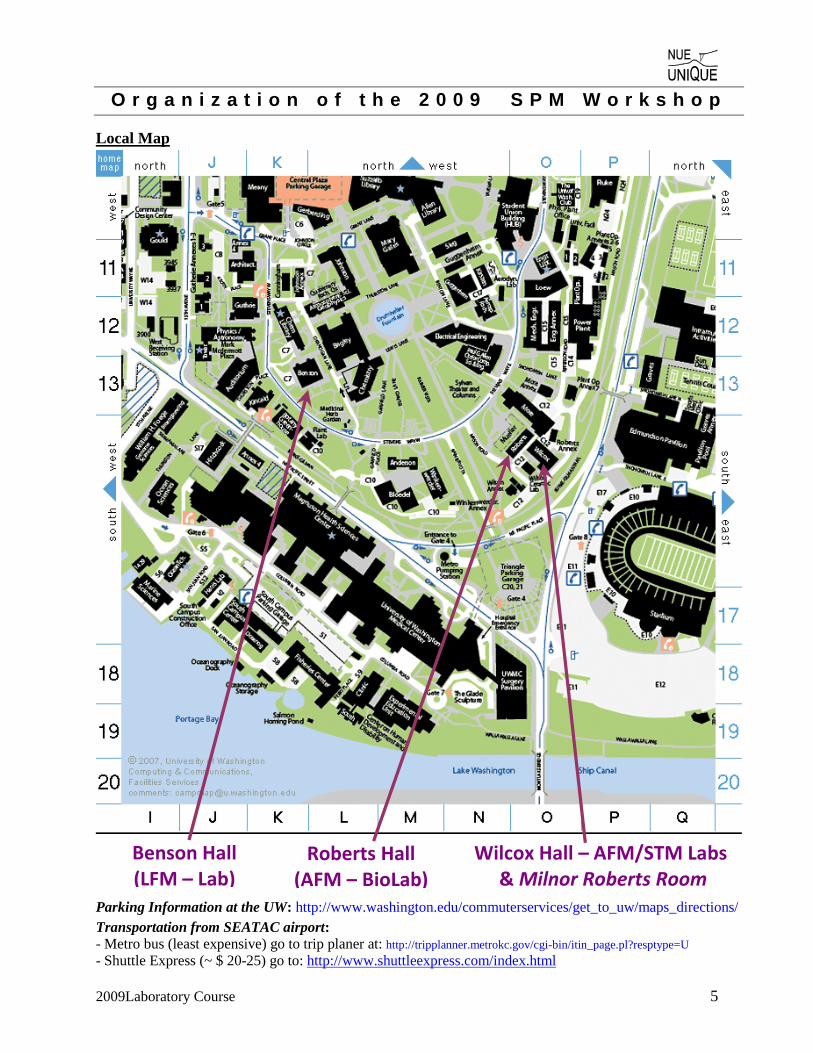
O r g a n i z a t i o n o f t h e 2 0 0 9 S P M W o r k s h o p
Local Map
Parking Information at the UW: http://www.washington.edu/commuterservices/get_to_uw/maps_directions/
Transportation from SEATAC airport: - Metro bus (least expensive) go to trip planer at: http://tripplanner.metrokc.gov/cgi-bin/itin_page.pl?resptype=U - Shuttle Express (~ $ 20-25) go to: http://www.shuttleexpress.com/index.html
Roberts Hall(AFM – BioLab)
Benson Hall (LFM – Lab)
Wilcox Hall – AFM/STM Labs& Milnor Roberts Room
2009Laboratory Course 6
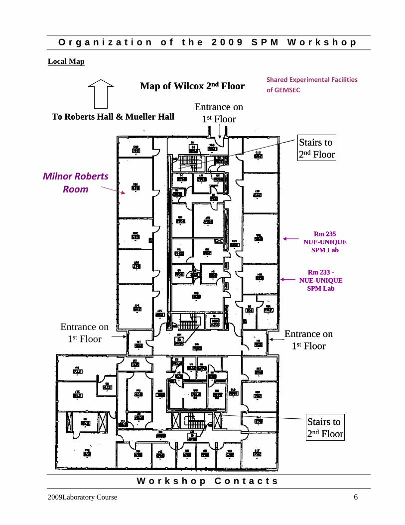
O r g a n i z a t i o n o f t h e 2 0 0 9 S P M W o r k s h o p
Local Map
Rm 235NUE-UNIQUE
SPM Lab
Rm 233 -NUE-UNIQUE
SPM Lab
Map of Wilcox 2nd Floor
To Roberts Hall & Mueller Hall
Entrance on1st Floor
Stairs to 2nd Floor
Stairs to 2nd Floor
Entrance on1st Floor
Entrance on1st Floor
Rm 235NUE-UNIQUE
SPM Lab
Rm 233 -NUE-UNIQUE
SPM Lab
Map of Wilcox 2nd Floor
To Roberts Hall & Mueller Hall
Entrance on1st Floor
Stairs to 2nd Floor
Stairs to 2nd Floor
Entrance on1st Floor
Entrance on1st Floor
W o r k s h o p C o n t a c t s
Shared Experimental Facilities of GEMSEC
Milnor Roberts Room

2009Laboratory Course 7 7
René M. Overney, Director NUE UNIQUE University of Washington, Seattle, WA 98195
[email protected] Phone: (206) 543-4353
Dan Knorr, Coordinator NUE UNIQUE University of Washington, Seattle, WA 98195
[email protected] Phone: (206) 616-6988
N U E U N I Q U E P A R T N E R S & S P O N S O R S
o UW - Genetically Engineered Materials Science &
Engineering Center GEMSEC (NSF-MRSEC)
o UW - Center for Nanotechnology (CNT)
o North Seattle Community College (NSCC), Seattle, WA
o Nanosurf, AG (Liestal, Switzerland)
NUE UNIQUE (Nanotechnology Undergraduate Education - Using Nanoscience Instrumentation for Quality Undergraduate Education), Grant 0634088, is a National Science Foundation sponsored program.

2009Laboratory Course 8
B i o g r a p h i c a l S k e t c h e s
Instructors
René Overney ([email protected], Prof. in Chemical Engineering) is known for his pioneering work in nanorheology and transport properties. His group has developed various SPM nano-characterization methods particularly applicable to polymer science and related technologies. The research of his group ranges from mesoscale material aspects in photonics, optoelectronics, electronic storage media, separation membranes, tribology to human implant technology. Overney coauthored one of the early textbooks in Nanoscience (Nanoscience, World Scientific 1998), and is teaching on the undergraduate and graduate level nanoscience related courses since 1996.
Mehmet Sarikaya ([email protected], Prof. in Materials Science and Engineering) is known for his pioneering efforts and ideas in Molecular Biomimetics. By merging recent advances in molecular biology and genetics with state-of-the-art engineering and nanocharacterization from the physical sciences, his and his collaborators’ goal is to shift the biomimetic materials science paradigm from imitating Nature to designing materials to perform artificial nanofunctions. It is the intent to combine Nature’s proven molecular tools, such as proteins, with synthetic nanoscale constructs to make molecular biomimetics a full-fledged methodology. To this end, at the Genetically Engineered Materials Science and Engineering Center, an NSF-MRSEC, Sarikaya is directing a multidisciplinary team with diverse expertise to genetically select inorganic-binding short polypeptides, tailoring them via molecular manipulation and bioinformatics to make heterofunctional molecular constructs and using them as synthesizers, assemblers, and molecular erectors in materials science and medicine.
Teaching Assistants
Dmitriy Khatayevich ([email protected]), currently a graduate in the group of Prof. Mehmet Sarikaya is working in the Genetically Engineered Materials Science and Engineering Center (GEMSEC). He is interested in applications of bio-inspired materials and molecular engineering. In his current project he uses the STM extensively.
Dan Knorr ([email protected]), currently a 4th year graduate student, is studying with Dr. René Overney and Dr. Alex Jen in the fields of atomic force microscopy and photonic materials. Dan earned B.S. and M.S. degrees in chemical engineering at Texas A&M University and then spent five years in the chemical industry as a process engineer with Chevron Phillips before returning to school to pursue a Ph.D.
Lakshmi Kocherlakota ([email protected]) is a 2nd year graduate student studying with Dr. René Overney. Lakshmi received a BS in Chemical Engineering and a M.S. from the Indian Institute of Science, Bangalore (IISc), India, and has five year work experience as engineer and scientist at GE Advanced Materials (GE ITC, India) and in Defense R&D Organization in India.
Chris So ([email protected]) graduated in 2006 with a BS from the Biochemistry program at the University of Washington. He is currently a graduate student in the Materials Science and Engineering Department working with Prof. Mehmet Sarikaya at the Genetically Engineered Materials Science and Engineering Center (GEMSEC). He is interested in bio-inspired materials and molecular biomimetics, particularly in using the AFM as a tool for their study.

2009Laboratory Course 9 9
A c k n o w l e d g m e n t
We gratefully acknowledge the lab unit development efforts by Michael Brasile, Yeechi Chen, Tomoko Gray, Ursula Koniges, Lakshmi S. Kocherlakota, Dan Knorr, Jason Killgore, Chris So, and Joseph Wei, and the logistic support efforts by Dr. Hanson Fong. We also like to express our gratitude to Dr. Ethan Allen (UW, CNT) and Dr. Tom Griffith (NSCC) for their support of this program from the very beginning. NUE UNIQUE is funded by the Nanotechnology Undergraduate Education (NUE) program of the National Science Foundation (Grant 06-538) and supported by GEMSEC (a UW based Mat. Res. and Eng. Center), Nanosurf AG (Switzerland) and nanoscience Instruments (AZ), and the Department of Chemical Engineering at the University of Washington.
2009Laboratory Course 10
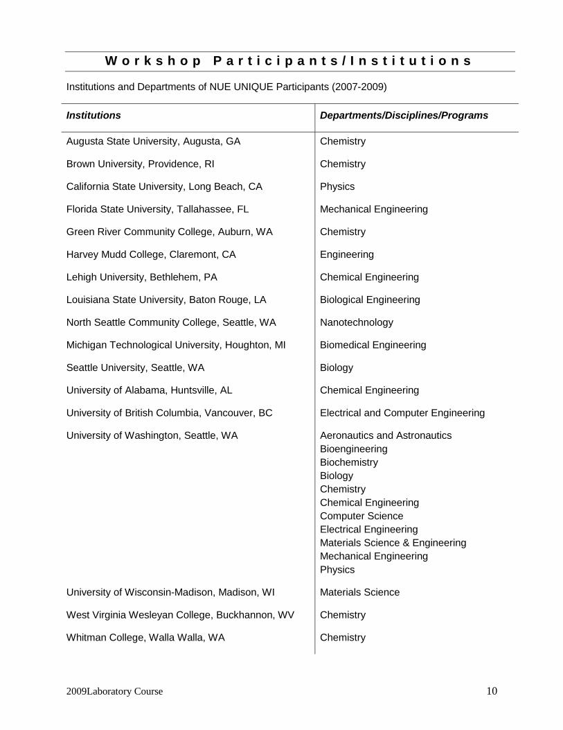
W o r k s h o p P a r t i c i p a n t s / I n s t i t u t i o n s
Institutions and Departments of NUE UNIQUE Participants (2007-2009)
Institutions Departments/Disciplines/Programs
Augusta State University, Augusta, GA Chemistry
Brown University, Providence, RI Chemistry
California State University, Long Beach, CA Physics
Florida State University, Tallahassee, FL Mechanical Engineering
Green River Community College, Auburn, WA Chemistry
Harvey Mudd College, Claremont, CA Engineering
Lehigh University, Bethlehem, PA Chemical Engineering
Louisiana State University, Baton Rouge, LA Biological Engineering
North Seattle Community College, Seattle, WA Nanotechnology
Michigan Technological University, Houghton, MI Biomedical Engineering
Seattle University, Seattle, WA Biology
University of Alabama, Huntsville, AL Chemical Engineering
University of British Columbia, Vancouver, BC Electrical and Computer Engineering
University of Washington, Seattle, WA Aeronautics and Astronautics Bioengineering Biochemistry Biology Chemistry Chemical Engineering Computer Science Electrical Engineering Materials Science & Engineering Mechanical Engineering Physics
University of Wisconsin-Madison, Madison, WI Materials Science
West Virginia Wesleyan College, Buckhannon, WV Chemistry
Whitman College, Walla Walla, WA Chemistry
LAB UNIT 1 Scanning Force Microscopy
2009LaboratoryProgram 11
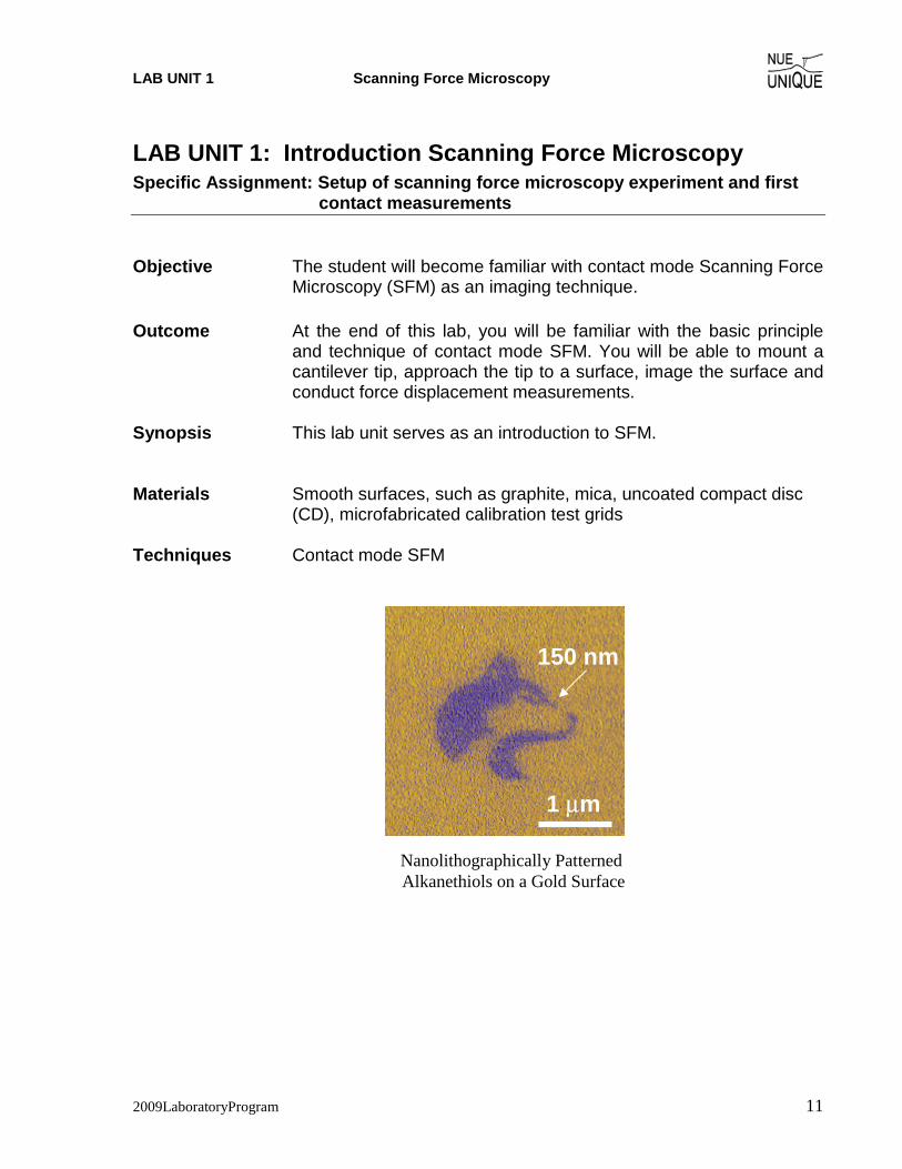
LAB UNIT 1: Introduction Scanning Force Microscopy Specific Assignment: Setup of scanning force microscopy experiment and first
contact measurements Objective The student will become familiar with contact mode Scanning Force
Microscopy (SFM) as an imaging technique. Outcome At the end of this lab, you will be familiar with the basic principle
and technique of contact mode SFM. You will be able to mount a cantilever tip, approach the tip to a surface, image the surface and conduct force displacement measurements.
Synopsis This lab unit serves as an introduction to SFM. Materials Smooth surfaces, such as graphite, mica, uncoated compact disc
(CD), microfabricated calibration test grids Techniques Contact mode SFM
1 μm
150 nm
Nanolithographically Patterned Alkanethiols on a Gold Surface
LAB UNIT 1 Scanning Force Microscopy
2009Laboratory Course 12
Table of Contents
1. Assignment............................................................................................... 13 2. Quiz ........................................................................................................... 14
2.1 Background Questions ........................................................................................ 14 3. Experimental Assignment ....................................................................... 16
3.1 Goal ..................................................................................................................... 16 3.2 Safety................................................................................................................... 16 3.3 Instrumental Setup............................................................................................... 16 3.4 Materials.............................................................................................................. 16 3.5 Experimental Procedure ...................................................................................... 16
4. Introduction to Scanning Force Microscopy (SFM) .............................. 19 4.1 Historic Perspectives ........................................................................................... 19 4.2 Scanning Force Microscopy (SFM) .................................................................... 20 4.2.1. Contact Mode ............................................................................................ 20 4.2.2. AC Mode Imaging..................................................................................... 21 4.2.3. Applied Force: Cantilever Deflection and Hooke’s Law.......................... 21 4.2.4. SFM Tips................................................................................................... 23 4.3 Dip-Pen Nanolithography (DPN)........................................................................ 25
References.................................................................................................... 26

LAB UNIT 1 Scanning Force Microscopy
2009LaboratoryProgram 13
1. Assignment In this lab, you will use the Scanning Force Microscope (SFM), also known as Atomic Force Microscope (AFM), as both an imaging tool, and a force measuring tool. As an imaging tool, you will use the most basic SFM imaging method: contact mode imaging. Employing force-displacement curves you will be measuring probe-sample forces and determine “true” normal loads.
1. (pre-lab) Read background information of Scanning Probe Microscopy in section 4 2. Take the quiz on your theoretical understanding in section 2 3. Learn on how to mount SFM tips 4. Image the samples provided 5. Conduct force displacement curves as function of the approach/retraction speed on three
different samples. Compare the adhesion forces.

LAB UNIT 1 Scanning Force Microscopy
2009Laboratory Course 14
2. Quiz
2.1 Background Questions
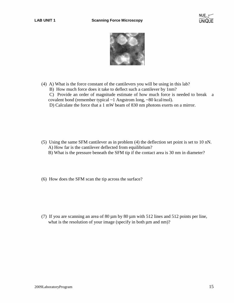
(1) How many hydrogen atoms would you have to line up to make one nanometer? (2) A student takes a SFM image like the one shown below to measure the size of some gold
nanoparticles attached to a surface. What are the dimensions of the nanoparticles?
(3) A student takes an SFM like the one shown below. Explain what has gone wrong.
LAB UNIT 1 Scanning Force Microscopy
2009LaboratoryProgram 15
(4) A) What is the force constant of the cantilevers you will be using in this lab? B) How much force does it take to deflect such a cantilever by 1nm? C) Provide an order of magnitude estimate of how much force is needed to break a
covalent bond (remember typical ~1 Angstrom long, ~80 kcal/mol). D) Calculate the force that a 1 mW beam of 830 nm photons exerts on a mirror. (5) Using the same SFM cantilever as in problem (4) the deflection set point is set to 10 nN. A) How far is the cantilever deflected from equilibrium? B) What is the pressure beneath the SFM tip if the contact area is 30 nm in diameter? (6) How does the SFM scan the tip across the surface? (7) If you are scanning an area of 80 μm by 80 μm with 512 lines and 512 points per line,
what is the resolution of your image (specify in both μm and nm)?
LAB UNIT 1 Scanning Force Microscopy
2009Laboratory Course 16
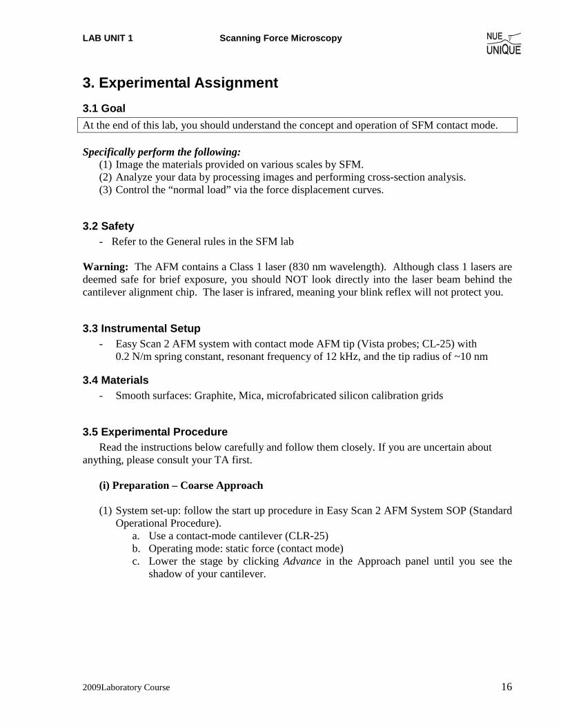
3. Experimental Assignment 3.1 Goal At the end of this lab, you should understand the concept and operation of SFM contact mode. Specifically perform the following:
(1) Image the materials provided on various scales by SFM. (2) Analyze your data by processing images and performing cross-section analysis. (3) Control the “normal load” via the force displacement curves.
3.2 Safety - Refer to the General rules in the SFM lab
Warning: The AFM contains a Class 1 laser (830 nm wavelength). Although class 1 lasers are deemed safe for brief exposure, you should NOT look directly into the laser beam behind the cantilever alignment chip. The laser is infrared, meaning your blink reflex will not protect you.
3.3 Instrumental Setup - Easy Scan 2 AFM system with contact mode AFM tip (Vista probes; CL-25) with
0.2 N/m spring constant, resonant frequency of 12 kHz, and the tip radius of ~10 nm
3.4 Materials - Smooth surfaces: Graphite, Mica, microfabricated silicon calibration grids
3.5 Experimental Procedure Read the instructions below carefully and follow them closely. If you are uncertain about
anything, please consult your TA first.
(i) Preparation – Coarse Approach (1) System set-up: follow the start up procedure in Easy Scan 2 AFM System SOP (Standard
Operational Procedure). a. Use a contact-mode cantilever (CLR-25) b. Operating mode: static force (contact mode) c. Lower the stage by clicking Advance in the Approach panel until you see the
shadow of your cantilever.
LAB UNIT 1 Scanning Force Microscopy
2009LaboratoryProgram 17
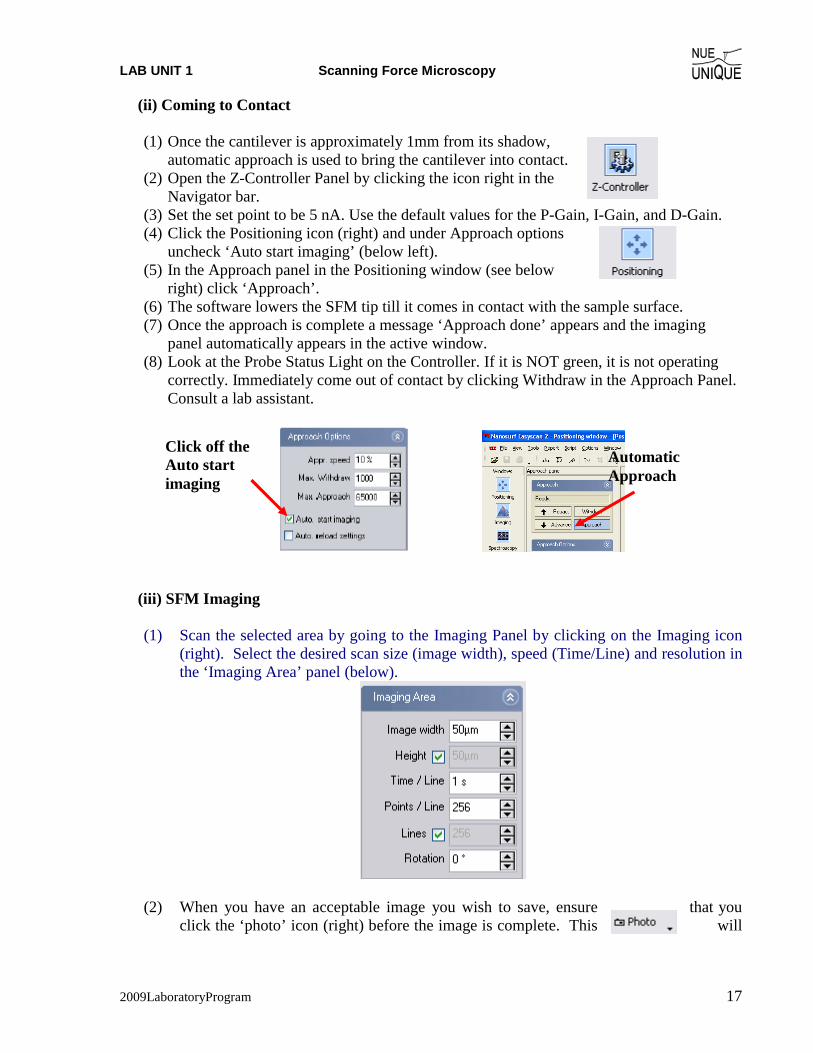
(ii) Coming to Contact (1) Once the cantilever is approximately 1mm from its shadow,
automatic approach is used to bring the cantilever into contact. (2) Open the Z-Controller Panel by clicking the icon right in the
Navigator bar. (3) Set the set point to be 5 nA. Use the default values for the P-Gain, I-Gain, and D-Gain. (4) Click the Positioning icon (right) and under Approach options
uncheck ‘Auto start imaging’ (below left). (5) In the Approach panel in the Positioning window (see below
right) click ‘Approach’. (6) The software lowers the SFM tip till it comes in contact with the sample surface. (7) Once the approach is complete a message ‘Approach done’ appears and the imaging
panel automatically appears in the active window. (8) Look at the Probe Status Light on the Controller. If it is NOT green, it is not operating
correctly. Immediately come out of contact by clicking Withdraw in the Approach Panel. Consult a lab assistant.
(iii) SFM Imaging (1) Scan the selected area by going to the Imaging Panel by clicking on the Imaging icon
(right). Select the desired scan size (image width), speed (Time/Line) and resolution in the ‘Imaging Area’ panel (below).
(2) When you have an acceptable image you wish to save, ensure that you
click the ‘photo’ icon (right) before the image is complete. This will
Automatic Approach
Click off the Auto start imaging
LAB UNIT 1 Scanning Force Microscopy
2009Laboratory Course 18
bring up a separate box with the completed image. To save the image go to File�Save As, create your own file on the desktop and save the image there.
(3) Process image and perform cross-section analysis using the options under the Tools. Keep in mind that you want to obtain the following information,
• Cross-section profile of surface structures • Dimensions of your structures (report average diameter and height with standard
deviation) • Determine the surface roughness
(iv) Procedure for force spectroscopy measurement
(1) Follow the procedure described in Easy Scan 2 force distance measurement SOP.
(2) Record for the each reading; a. Adhesion force in units of nm, b. The temperature and the humidity c. Any other observations that might be relevant in interpreting the results
(v) AFM shut down
(1) Follow the Easy Scan 2 AFM System SOP Shutdown Procedure
LAB UNIT 1 Scanning Force Microscopy
2009LaboratoryProgram 19
4. Introduction to Scanning Force Microscopy (SFM)
Table of Contents: 4.1 Historic Perspectives ..................................................................................................................... 19 4.2 Scanning Force Microscopy (SFM) .............................................................................................. 20 4.2.1. Contact Mode ......................................................................................................................... 20 4.2.2. AC Mode Imaging.................................................................................................................. 21 4.2.3. Applied Force: Cantilever Deflection and Hooke’s Law ....................................................... 21 4.2.4. SFM Tips................................................................................................................................ 22 4.3 Dip-Pen Nanolithography (DPN) .................................................................................................. 25
References ........................................................................................................................................... 26
4.1 Historic Perspectives
In 1982, Gerd Binnig and Heinrich Rohrer of IBM in Rüschlikon (Switzerland) invented scanning tunneling microscopy (STM). Although STM is not the focus of this lab, it is the ancestor of all the variations of scanning probe microscopy (SPM) that followed: although the mechanism of image contrast may vary, the idea of building up an image by scanning a very sharp probe across a surface has endured. As the name suggests, STM scans a sharp tip across a surface while recording the quantum mechanical tunneling current to generate the image. STM is capable of making extremely high resolution (atomic resolution) images of surfaces and has been extremely useful in many branches of science and engineering. For their invention, Binnig and Rohrer were awarded the Nobel Prize in Physics in 19861.
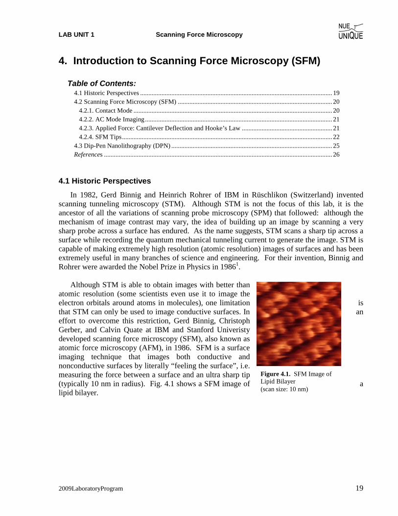
Although STM is able to obtain images with better than
atomic resolution (some scientists even use it to image the electron orbitals around atoms in molecules), one limitation is that STM can only be used to image conductive surfaces. In an effort to overcome this restriction, Gerd Binnig, Christoph Gerber, and Calvin Quate at IBM and Stanford Univeristy developed scanning force microscopy (SFM), also known as atomic force microscopy (AFM), in 1986. SFM is a surface imaging technique that images both conductive and nonconductive surfaces by literally “feeling the surface”, i.e. measuring the force between a surface and an ultra sharp tip (typically 10 nm in radius). Fig. 4.1 shows a SFM image of a lipid bilayer.
Figure 4.1. SFM Image of Lipid Bilayer (scan size: 10 nm)
LAB UNIT 1 Scanning Force Microscopy
2009Laboratory Course 20
4.2 Scanning Force Microscopy (SFM)
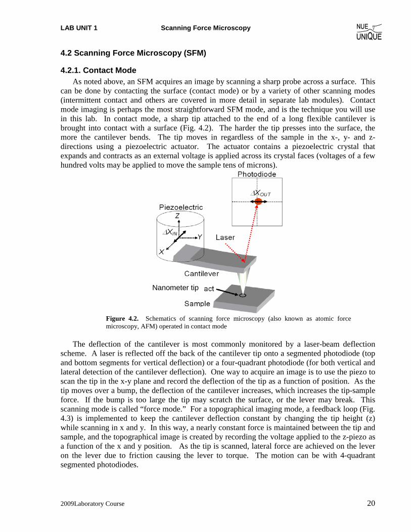
4.2.1. Contact Mode As noted above, an SFM acquires an image by scanning a sharp probe across a surface. This
can be done by contacting the surface (contact mode) or by a variety of other scanning modes (intermittent contact and others are covered in more detail in separate lab modules). Contact mode imaging is perhaps the most straightforward SFM mode, and is the technique you will use in this lab. In contact mode, a sharp tip attached to the end of a long flexible cantilever is brought into contact with a surface (Fig. 4.2). The harder the tip presses into the surface, the more the cantilever bends. The tip moves in regardless of the sample in the x-, y- and z-directions using a piezoelectric actuator. The actuator contains a piezoelectric crystal that expands and contracts as an external voltage is applied across its crystal faces (voltages of a few hundred volts may be applied to move the sample tens of microns).
Figure 4.2. Schematics of scanning force microscopy (also known as atomic force microscopy, AFM) operated in contact mode
The deflection of the cantilever is most commonly monitored by a laser-beam deflection
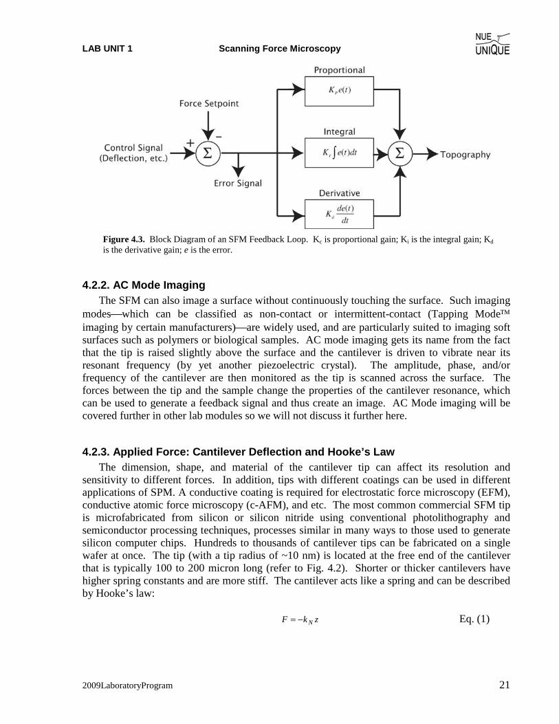
scheme. A laser is reflected off the back of the cantilever tip onto a segmented photodiode (top and bottom segments for vertical deflection) or a four-quadrant photodiode (for both vertical and lateral detection of the cantilever deflection). One way to acquire an image is to use the piezo to scan the tip in the x-y plane and record the deflection of the tip as a function of position. As the tip moves over a bump, the deflection of the cantilever increases, which increases the tip-sample force. If the bump is too large the tip may scratch the surface, or the lever may break. This scanning mode is called “force mode.” For a topographical imaging mode, a feedback loop (Fig. 4.3) is implemented to keep the cantilever deflection constant by changing the tip height (z) while scanning in x and y. In this way, a nearly constant force is maintained between the tip and sample, and the topographical image is created by recording the voltage applied to the z-piezo as a function of the x and y position. As the tip is scanned, lateral force are achieved on the lever on the lever due to friction causing the lever to torque. The motion can be with 4-quadrant segmented photodiodes.
Nanometer tip
LAB UNIT 1 Scanning Force Microscopy
2009LaboratoryProgram 21
Figure 4.3. Block Diagram of an SFM Feedback Loop. Kc is proportional gain; Ki is the integral gain; Kd is the derivative gain; e is the error.
4.2.2. AC Mode Imaging The SFM can also image a surface without continuously touching the surface. Such imaging
modes⎯which can be classified as non-contact or intermittent-contact (Tapping Mode™ imaging by certain manufacturers)⎯are widely used, and are particularly suited to imaging soft surfaces such as polymers or biological samples. AC mode imaging gets its name from the fact that the tip is raised slightly above the surface and the cantilever is driven to vibrate near its resonant frequency (by yet another piezoelectric crystal). The amplitude, phase, and/or frequency of the cantilever are then monitored as the tip is scanned across the surface. The forces between the tip and the sample change the properties of the cantilever resonance, which can be used to generate a feedback signal and thus create an image. AC Mode imaging will be covered further in other lab modules so we will not discuss it further here.
4.2.3. Applied Force: Cantilever Deflection and Hooke’s Law The dimension, shape, and material of the cantilever tip can affect its resolution and
sensitivity to different forces. In addition, tips with different coatings can be used in different applications of SPM. A conductive coating is required for electrostatic force microscopy (EFM), conductive atomic force microscopy (c-AFM), and etc. The most common commercial SFM tip is microfabricated from silicon or silicon nitride using conventional photolithography and semiconductor processing techniques, processes similar in many ways to those used to generate silicon computer chips. Hundreds to thousands of cantilever tips can be fabricated on a single wafer at once. The tip (with a tip radius of ~10 nm) is located at the free end of the cantilever that is typically 100 to 200 micron long (refer to Fig. 4.2). Shorter or thicker cantilevers have higher spring constants and are more stiff. The cantilever acts like a spring and can be described by Hooke’s law:
zkF N−= Eq. (1)

LAB UNIT 1 Scanning Force Microscopy
2009Laboratory Course 22
where F is the force, kN is the normal spring constant, and z is the cantilever normal deflection. Typical spring constants available on commercially manufactured SFM cantilevers range from 0.01 N/m to 75 N/m. This enables forces as small as 10-9 N to be measured in liquids or an ultra-dry environment with the SFM. Analogous, lateral forces acting on the lever can be expressed as the product between a lateral spring constant kx and a lateral deflection x.
For a bar-shaped cantilever with length L, width W and thickness t, and an integrated tip of length r, the normal and lateral spring constants, kL and kx, are related to the material stiffnesses, as
3
3
4LEWtkN = and 2
3
3LrGWtk x = .
where E and G respresent the normal Young’s modulus and the shear modulus, respectively. The thickness of the cantilever, typically poorly defined by the manufacturers, can be
determined from the first resonance frequency of the "free" cantilever using the following empirical equation:2
( ) EL
.ft ρπ 12
87510412 2
21=
The Young's modulus and density of silicon cantilevers are around E = 1.69×10¹¹ N/m2 and ρ=2.33×10³ kg/m3.2
4.2.4. SFM Tips The lateral imaging resolution of SFM is intrinsically limited by the sharpness of the
cantilever. Most commercial cantilevers have a tip with a 10 nm radius of curvature, although more exotic probes (such as those tipped with carbon nanotubes) are also available. Keep in mind that the resolution is also limited by the scanning parameters. For instance, if you take a 10x10 micron scan with a resolution of only 256x256 points, the size of each image pixel represents a lateral distance of 1x10⁻⁶ m / 256 = 39 nm.
As SFM images are generated by scanning a physical tip across the surface, this can lead to several image artifacts. One type of imaging artifact results from tip convolution. When the tip size is larger than the imaging feature size, the resulting image will be dominated by the shape of the tip. In this case, the observed features from the topography images will have very similar shapes despite the fact that the real features might be different (think of it as taking a picture of the tip with each of the surface features). Fig 4.4 shows two different sized tips scanned over a substrate with both small and large features. Also, damaged tips can often lead to distorted images. A tip with a piece of dirt stuck to it, or one that has been broken near the end can yield, for instance, doubled features as illustrated in Fig 4.5. One way to check for tip-induced artifacts is to rotate the scan angle by 90 degrees. If the shapes you are seeing do not rotate, the tip might be damaged!

LAB UNIT 1 Scanning Force Microscopy
2009LaboratoryProgram 23
Figure 4.4. Limitations of Tip Size. (Top) The large tip is much bigger than the small substrate feature. Each circle on the figure represents the position of the z-piezo recorded by the SFM as it moves across the sample. (Center) A small tip tracks both surface features better. (Bottom) The two line traces (large tip is dashed blue; small tip dotted green) from each tip are shown with the actual surface topography.
LAB UNIT 1 Scanning Force Microscopy
2009Laboratory Course 24
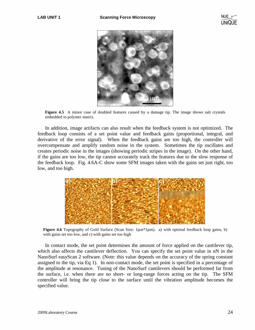
Figure 4.5 A minor case of doubled features caused by a damage tip. The image shows salt crystals embedded in polymer matrix.
In addition, image artifacts can also result when the feedback system is not optimized. The
feedback loop consists of a set point value and feedback gains (proportional, integral, and derivative of the error signal). When the feedback gains are too high, the controller will overcompensate and amplify random noise in the system. Sometimes the tip oscillates and creates periodic noise in the images (showing periodic stripes in the image). On the other hand, if the gains are too low, the tip cannot accurately track the features due to the slow response of the feedback loop. Fig. 4.6A-C show some SFM images taken with the gains set just right, too low, and too high.
Figure 4.6 Topography of Gold Surface (Scan Size: 1μm*1μm). a) with optimal feedback loop gains, b) with gains set too low, and c) with gains set too high
In contact mode, the set point determines the amount of force applied on the cantilever tip,
which also affects the cantilever deflection. You can specify the set point value in nN in the NanoSurf easyScan 2 software. (Note: this value depends on the accuracy of the spring constant assigned to the tip, via Eq 1). In non-contact mode, the set point is specified in a percentage of the amplitude at resonance. Tuning of the NanoSurf cantilevers should be performed far from the surface, i.e. when there are no short- or long-range forces acting on the tip. The SFM controller will bring the tip close to the surface until the vibration amplitude becomes the specified value.
5 μm
LAB UNIT 1 Scanning Force Microscopy
2009LaboratoryProgram 25
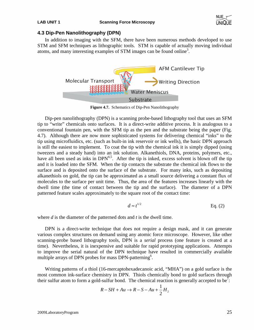
4.3 Dip-Pen Nanolithography (DPN) In addition to imaging with the SFM, there have been numerous methods developed to use
STM and SFM techniques as lithographic tools. STM is capable of actually moving individual atoms, and many interesting examples of STM images can be found online3.
Figure 4.7. Schematics of Dip-Pen Nanolithography
Dip-pen nanolithography (DPN) is a scanning probe-based lithography tool that uses an SFM
tip to “write” chemicals onto surfaces. It is a direct-write additive process. It is analogous to a conventional fountain pen, with the SFM tip as the pen and the substrate being the paper (Fig. 4.7). Although there are now more sophisticated systems for delivering chemical “inks” to the tip using microfluidics, etc. (such as built-in ink reservoir or ink wells), the basic DPN approach is still the easiest to implement. To coat the tip with the chemical ink it is simply dipped (using tweezers and a steady hand) into an ink solution. Alkanethiols, DNA, proteins, polymers, etc., have all been used as inks in DPN4,5. After the tip is inked, excess solvent is blown off the tip and it is loaded into the SFM. When the tip contacts the substrate the chemical ink flows to the surface and is deposited onto the surface of the substrate. For many inks, such as depositing alkanethiols on gold, the tip can be approximated as a small source delivering a constant flux of molecules to the surface per unit time. Thus, the area of the features increases linearly with the dwell time (the time of contact between the tip and the surface). The diameter of a DPN patterned feature scales approximately to the square root of the contact time:
d ≈ t1/2 Eq. (2) where d is the diameter of the patterned dots and t is the dwell time.
DPN is a direct-write technique that does not require a design mask, and it can generate various complex structures on demand using any atomic force microscope. However, like other scanning-probe based lithography tools, DPN is a serial process (one feature is created at a time). Nevertheless, it is inexpensive and suitable for rapid prototyping applications. Attempts to improve the serial natural of the DPN technique have resulted in commercially available multiple arrays of DPN probes for mass DPN-patterning6.
Writing patterns of a thiol (16-mercaptohexadecanoic acid, “MHA”) on a gold surface is the most common ink-surface chemistry in DPN. Thiols chemically bond to gold surfaces through their sulfur atom to form a gold-sulfur bond. The chemical reaction is generally accepted to be7:
R − SH + Au → R − S − Au +12
H 2
LAB UNIT 1 Scanning Force Microscopy
2009Laboratory Course 26
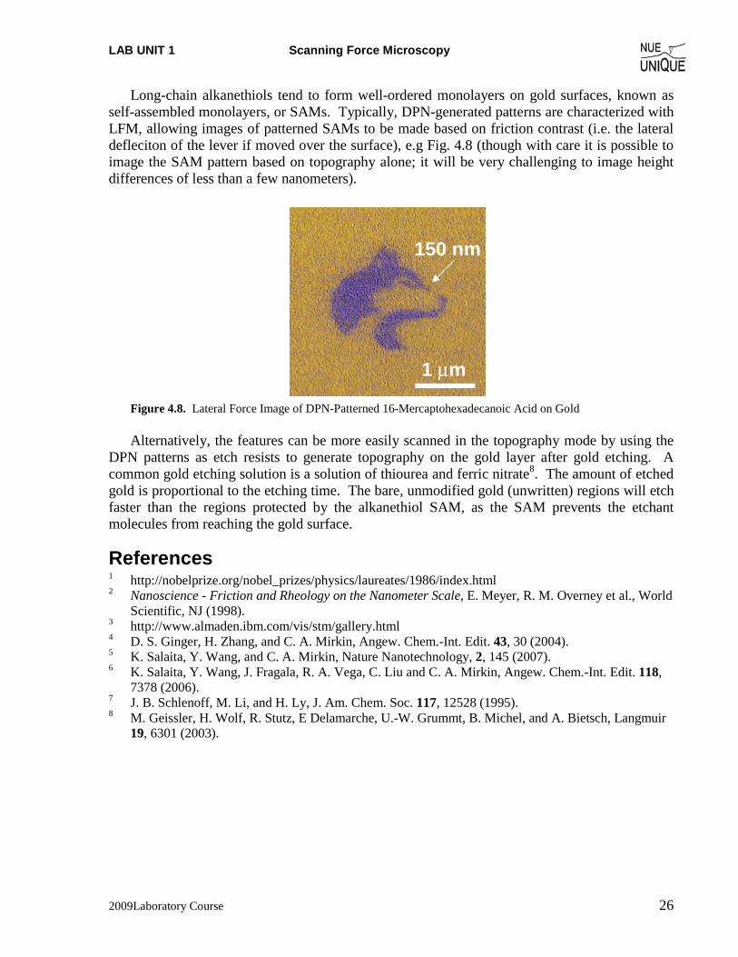
Long-chain alkanethiols tend to form well-ordered monolayers on gold surfaces, known as self-assembled monolayers, or SAMs. Typically, DPN-generated patterns are characterized with LFM, allowing images of patterned SAMs to be made based on friction contrast (i.e. the lateral defleciton of the lever if moved over the surface), e.g Fig. 4.8 (though with care it is possible to image the SAM pattern based on topography alone; it will be very challenging to image height differences of less than a few nanometers).
Figure 4.8. Lateral Force Image of DPN-Patterned 16-Mercaptohexadecanoic Acid on Gold
Alternatively, the features can be more easily scanned in the topography mode by using the DPN patterns as etch resists to generate topography on the gold layer after gold etching. A common gold etching solution is a solution of thiourea and ferric nitrate8. The amount of etched gold is proportional to the etching time. The bare, unmodified gold (unwritten) regions will etch faster than the regions protected by the alkanethiol SAM, as the SAM prevents the etchant molecules from reaching the gold surface.
References 1 http://nobelprize.org/nobel_prizes/physics/laureates/1986/index.html 2 Nanoscience - Friction and Rheology on the Nanometer Scale, E. Meyer, R. M. Overney et al., World
Scientific, NJ (1998). 3 http://www.almaden.ibm.com/vis/stm/gallery.html 4 D. S. Ginger, H. Zhang, and C. A. Mirkin, Angew. Chem.-Int. Edit. 43, 30 (2004). 5 K. Salaita, Y. Wang, and C. A. Mirkin, Nature Nanotechnology, 2, 145 (2007). 6 K. Salaita, Y. Wang, J. Fragala, R. A. Vega, C. Liu and C. A. Mirkin, Angew. Chem.-Int. Edit. 118,
7378 (2006). 7 J. B. Schlenoff, M. Li, and H. Ly, J. Am. Chem. Soc. 117, 12528 (1995). 8 M. Geissler, H. Wolf, R. Stutz, E Delamarche, U.-W. Grummt, B. Michel, and A. Bietsch, Langmuir
19, 6301 (2003).
1 μm
150 nm

LAB UNIT 2 Protein Adsorption and Scanning in Fluid-Mode
2009LaboratoryProgram 27
LAB UNIT 2: Non-Contact Scanning Force Microscopy in Air
and Liquid Environment Specific Assignment: Protein Adsorption Kinetics Objective In this lab unit students are characterizing protein-material
interactions using intermittent non-contact (NC) scanning force microscopy (SFM) in both fluid medium and in air to quantify complex surface adsorption processes. The material analyzed is graphite adsorbed with a blood clotting protein, fibrinogen (Fb), to mimic a bio-response to prosthetic heart valve devices.
Outcome Gain insight into macromolecular surface interaction at the
molecular level and its role in understanding/improving the field of engineered biomaterials. Learn about proteins and adsorption from a physiological perspective, and to quantify equilibrium adsorption constant Ka as well as the Gibbs Free Energy of adsorption using high resolution SFM and the Langmuir model.
Synopsis Implant rejection by the body accounts for a large percentage of
preventable surgeries occurring in modern medicine today. At the earliest stages of the immune response, foreign bodies are marked by clotting agents such as fibrinogen (Fb) which signals larger platelets and white blood cells to initiate a response pathway and
eventually to isolate it from the rest of the body. By understanding the initial stage of protein-solid interactions and engineering materials to camouflage them from early protein adsorption, the immune response can be bypassed and long-term complications avoided by the implant patient. This lab seeks to characterize protein-
solid interactions via SFM imaging in order to understand the adsorption behavior of fibrinogen in real time for the purpose of simulating a graphitic carbon modern prosthetic heart valve. Fibrinogen a blood clotting protein,
adsorbed on graphite imaged by intermittent NC-SFM

LAB UNIT 2 Protein Adsorption and Scanning in Fluid-Mode
2009LaboratoryProgram 28
Table of Contents 1. Assignment................................................................................................... 29 2. Quiz – Preparation for the Experiment....................................................... 30
Theoretical Questions................................................................................................ 30 Prelab Quiz ................................................................................................................ 30
3. Experimental Assignment ........................................................................... 32 Goal ........................................................................................................................... 32 Safety......................................................................................................................... 32 Instrumental Setup..................................................................................................... 32 Materials.................................................................................................................... 32 Experimental Procedure ............................................................................................ 33
4. Background: Fibrinogen’s Role in Biomaterial Response and Protein-Solid Interactions................................................................................................... 40
Brief Overview on Blood Clotting ............................................................................ 40 Fibrinogen Structure and Functioning Mechanism................................................... 42 Bio-Response toward Implant Devices and Foreign Bodies..................................... 43 Implant Material Design............................................................................................ 44 Characterization of Adsorption Processes................................................................. 47 Artificial Nose or Biosensor...................................................................................... 50 References ................................................................................................................. 51
5. Appendix....................................................................................................... 52 Simple Harmonic Motion.......................................................................................... 52 AC-Mode Imaging .................................................................................................... 54
LAB UNIT 2 Protein Adsorption and Scanning in Fluid-Mode
2009LaboratoryProgram 29
1. Assignment The assignment is to use the SFM in both air and a dynamic fluid medium to observe the binding morphology of a common blood clotting factor towards a graphitic surface. Further, we will seek to quantify this adsorption in order to characterize its binding modality based on the observable surface coverage from resulting SFM images. In fluid mode, scanning will begin in buffer solution while the protein is introduced and observed to bind over time. To quantify surface coverage trends, we will scan previously prepared samples which have been exposed to protein solutions, at equilibrium, of increasing concentrations in air for enhanced resolution. The module’s emphasis will be on understanding the precedent for such experiments and their application for improving engineered biomaterials. The steps are outlined here:
1. Familiarize yourself with the background information provided in Section 4. 2. Test your background knowledge with the provided Quiz in Section 2. 3. Conduct the fluid-mode and in-air experiments in Section 3. Follow the step-by-step
experimental procedure. 4. Analyze your data as described in Section 3. 5. Finally, provide a report with the following information:
(i) Results section: In this section you show your data and discuss instrumental details (i.e., limitations) and the quality of your data (error analysis).
(ii) Discussion section: In this section you discuss and analyze your data in the light of the provided background information.
It is also appropriate to discuss sections (i) and (ii) together. (iii) Summary: Here you summarize your findings and provide comments on how your
results would affect any future SFM work you may do. The report is evaluated based on the quality of the discussion and the integration of your experimental data and the provided theory. You are encouraged to discuss results that are unexpected. It is important to include discussions on the causes for discrepancies and inconsistencies in the data.
LAB UNIT 2 Protein Adsorption and Scanning in Fluid-Mode
2009LaboratoryProgram 30
2. Quiz – Preparation for the Experiment Background Questions Biology Background 1. Explain, briefly, the role(s) of fibrinogen in the context of implant rejection. 2. Why are smooth surfaces preferred over rough ones as implant coatings? 3. Why don’t proteins generally aggregate in aqueous solutions? Why do they aggregate on surfaces? 4. What is the difference between the ‘intrinsic’ bio-response and the ‘extrinsic’ one? 5. Why is graphite the material of choice for heart valve prostheses? 6. Stoney’s formula (Klein, C. A. J. Appl. Phys. 2000, 88, 5487)
( ) zELD Δ
−⎟⎠
⎞⎜⎝
⎛=ν
σ13
1 2
relates the tensile surface stress σ to the normal deflection Δz measured at the front of the cantilever. With the cantilever spring constant kN, given as
3
3
4LEWDk N = ,
derive the function σ(kN).
LAB UNIT 2 Protein Adsorption and Scanning in Fluid-Mode
2009LaboratoryProgram 31
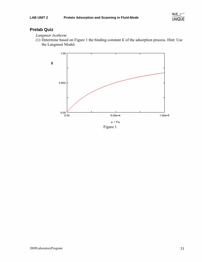
Prelab Quiz Langmuir Isotherm (1) Determine based on Figure 1 the binding constant K of the adsorption process. Hint: Use
the Langmuir Model.
Figure 1
LAB UNIT 2 Protein Adsorption and Scanning in Fluid-Mode
2009LaboratoryProgram 32
3. Experimental Assignment Goal Following the step-by-step instructions below, determine the adsorption kinetics of fibrinogen on highly oriented pyrolytic graphite (HOPG) in phosphate buffer solution. This experiment will be performed in AC-mode (intermittent non contact (NC) mode) both in air using dried samples and in liquid to obtain ‘real time’ data. Analyze and discuss the data with the background information provided in Section 4. Provide a written report of this experiment. Specifically provide answers to the following questions:
(1) What morphologies do you notice on the surface? Where does the protein seem to bind first (i.e. at earlier times)? Why is this?
(2) Is it easier to determine protein surface coverage from a topography image or a phase contrast image? Why?
(3) According to the analysis, what was (a) Κa and (b) θmax for the measurements taken in air?
(4) If possible, according to the analysis of measurements taken in liquid what was (a) θinf and (b) τ ?
(5) Compare your results the results previously reported[1] how are your results different/similar? Discuss your findings and what experimental aspects may be different between your study and the literature
(6) Why is the resonance frequency in liquid much different from that in air? If possible, report your values for both liquid and air.
Safety - Wear safety glasses. - Refer to the General rules in the SFM lab. - Wear gloves when handling Fibrinogen in solution. - Take particular care to avoid using too much liquid in the liquid mode experiment as this
could damage the instrument and cause an electrical shock
Instrumental Setup - Easy Scan 2 SFM system with Forrce Modulation tip (FMR) 3 N/m spring constant. - Nanosurf Easyscan 2 Flex AFM system with Nanosensor or Vista FMR cantilevers with
~3 N/m spring constant.
Materials - Samples: 6 pieces of HOPG that were exposed to Fibrinogen solution in PBS (provided)
for 1.5 hrs. Concentrations of protein solution were: 0.05 µg/mL, 0.667 µg/mL, 3.33 µg/mL, 30 µg/mL and 100 µg/mL.
- A separate HOPG sample for use in liquid mode - Double sided tape (to cleave graphite and secure graphite samples) - Pipetter (100μL) with pipette tips
LAB UNIT 2 Protein Adsorption and Scanning in Fluid-Mode
2009LaboratoryProgram 33
- 10mL of ethanol to sterilize pipette tips - 50mL of PBS - 1mL of a 1mg/mL solution of Fibrinogen in PBS - Vista FMR probes - Nanosensors PPP-FMR probes - Tweezers
Experimental Procedure Read the instructions below carefully and follow them closely. They will provide you with information about (i) preparation of the experiment, (ii) the procedure for dry dynamic mode imaging, (iii) the procedure for liquid dynamic mode imaging, and (iv) how to conduct the data analysis.
(i) Preparation of the experiment
(1) Dry dynamic mode system set-up: (This part will be performed with a TA). a. System set-up
i. Remove the scan head from the sample stage. ii. Load a Vista FMR cantilever with a spring constant of 3 N/m on the EasyScan 2.
iii. Position one of the provided dry graphite samples with Fibrinogen on the sample stage and electrically ground the sample.
iv. Carefully place the scan head onto the sample stage ensuring by watching the video feed that you have sufficient clearance to avoid crashing the tip into the surface. Carefully adjust the height of the scan head such that the tip is ~ 1mm from the surface.
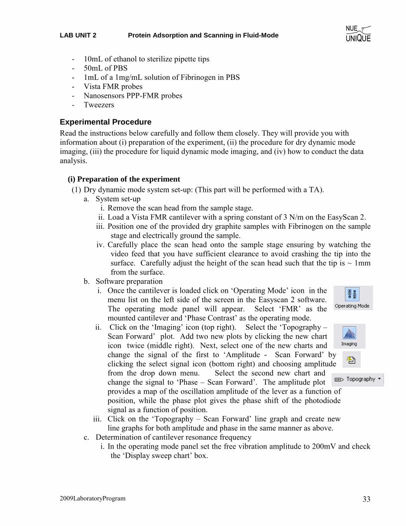
b. Software preparation i. Once the cantilever is loaded click on ‘Operating Mode’ icon in the
menu list on the left side of the screen in the Easyscan 2 software. The operating mode panel will appear. Select ‘FMR’ as the mounted cantilever and ‘Phase Contrast’ as the operating mode.
ii. Click on the ‘Imaging’ icon (top right). Select the ‘Topography – Scan Forward’ plot. Add two new plots by clicking the new chart icon twice (middle right). Next, select one of the new charts and change the signal of the first to ‘Amplitude - Scan Forward’ by clicking the select signal icon (bottom right) and choosing amplitude from the drop down menu. Select the second new chart and change the signal to ‘Phase – Scan Forward’. The amplitude plot provides a map of the oscillation amplitude of the lever as a function of position, while the phase plot gives the phase shift of the photodiode signal as a function of position.
iii. Click on the ‘Topography – Scan Forward’ line graph and create new line graphs for both amplitude and phase in the same manner as above.
c. Determination of cantilever resonance frequency i. In the operating mode panel set the free vibration amplitude to 200mV and check
the ‘Display sweep chart’ box.
LAB UNIT 2 Protein Adsorption and Scanning in Fluid-Mode
2009LaboratoryProgram 34
ii. Click the ‘Set’ button just below the vibration frequency box. The software will automatically perform two sweeps to find the resonance frequency. Two plots will appear. Examine them to ensure that a peak frequency of reasonable height (>100mV) was found.
iii. The probe status light should be red before this process and yellow afterward.
(2) Liquid mode system set up: (This part will be performed with a TA).
a. System set-up: i. Using double sided tape, cleave the graphite to be used for liquid mode
imaging. ii. Remove the SFM head from the sample stage and set it upside down on a
secure surface. iii. Crank the sample stage down until it is fully lowered and load the freshly
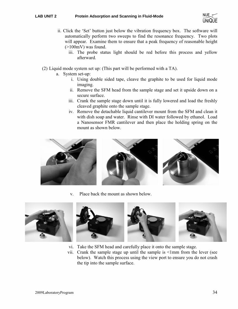
cleaved graphite onto the sample stage. iv. Remove the detachable liquid cantilever mount from the SFM and clean it
with dish soap and water. Rinse with DI water followed by ethanol. Load a Nanosensor FMR cantilever and then place the holding spring on the mount as shown below.
v. Place back the mount as shown below.
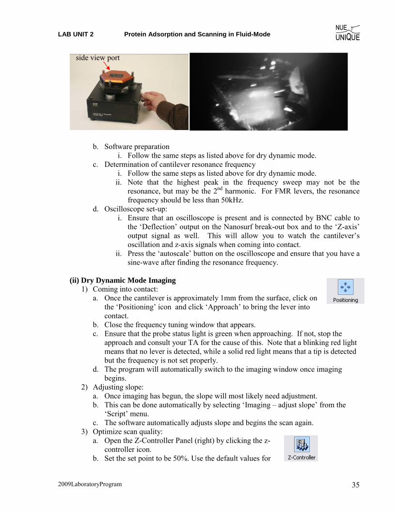
vi. Take the SFM head and carefully place it onto the sample stage. vii. Crank the sample stage up until the sample is <1mm from the lever (see
below). Watch this process using the view port to ensure you do not crash the tip into the sample surface.
LAB UNIT 2 Protein Adsorption and Scanning in Fluid-Mode
2009LaboratoryProgram 35
b. Software preparation i. Follow the same steps as listed above for dry dynamic mode.
c. Determination of cantilever resonance frequency i. Follow the same steps as listed above for dry dynamic mode.
ii. Note that the highest peak in the frequency sweep may not be the resonance, but may be the 2nd harmonic. For FMR levers, the resonance frequency should be less than 50kHz.
d. Oscilloscope set-up: i. Ensure that an oscilloscope is present and is connected by BNC cable to
the ‘Deflection’ output on the Nanosurf break-out box and to the ‘Z-axis’ output signal as well. This will allow you to watch the cantilever’s oscillation and z-axis signals when coming into contact.
ii. Press the ‘autoscale’ button on the oscilloscope and ensure that you have a sine-wave after finding the resonance frequency.
(ii) Dry Dynamic Mode Imaging
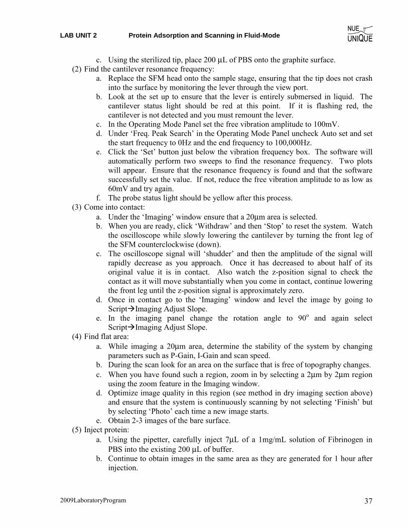
1) Coming into contact: a. Once the cantilever is approximately 1mm from the surface, click on
the ‘Positioning’ icon and click ‘Approach’ to bring the lever into contact.
b. Close the frequency tuning window that appears. c. Ensure that the probe status light is green when approaching. If not, stop the
approach and consult your TA for the cause of this. Note that a blinking red light means that no lever is detected, while a solid red light means that a tip is detected but the frequency is not set properly.
d. The program will automatically switch to the imaging window once imaging begins.
2) Adjusting slope: a. Once imaging has begun, the slope will most likely need adjustment. b. This can be done automatically by selecting ‘Imaging – adjust slope’ from the
‘Script’ menu. c. The software automatically adjusts slope and begins the scan again.
3) Optimize scan quality: a. Open the Z-Controller Panel (right) by clicking the z-
controller icon. b. Set the set point to be 50%. Use the default values for
side view port

LAB UNIT 2 Protein Adsorption and Scanning in Fluid-Mode
2009LaboratoryProgram 36
the P-Gain and I-Gain. c. In the Imaging Panel, change the image width to 2μm and ensure that the
resolution is set to 256. d. Vary the set point, P-Gain, I-Gain and time/line values to optimize the image
quality according to the following guidelines: i. Faster scan speeds (lower time/line values) generally require higher gains. ii. Excessively high gains cause the controller to ring, resulting in very noisy
amplitude and topography signals. iii. Very large surface features generally require higher gains or higher amplitude
or slower scan speed. iv. Noisy measurements may improve with increased set point, but very high set
points may result in coming out of contact. You may also employ the minimum force trick, that is, increase the set point (%) until you are out of contact and then decrease it again until a reasonable image is obtained. This results in using the minimum force.
4) Obtain images: a. Once scan quality is acceptable complete the scan by clicking on the ‘Finish’
icon. b. If the completed image looks good, click ‘Photo’ and save the image. c. Each image should be in a different area of the sample. To move to a different
area, simply select random values (from -20 to 20 μm) and input these into the ‘Image X-Pos’ and ‘Image Y-Pos’ fields in the imaging panel. Alternatively, you may withdraw the cantilever under the ‘Positioning’ window and use the translation stage to move to a new area of the sample surface. Be sure to ‘Approach’ again after moving.
d. Click ‘Start’ to begin a new image. Repeat slope adjustment and image optimization as necessary.
e. Obtain at least three images for each sample. 5) Change sample:
a. Once all images have been obtained for that sample, go to the ‘Positioning’ window and click ‘Withdraw’.
b. Once the cantilever is well off the surface, click ‘Retract’ and raise the tip farther (~3 mm off the surface).
c. Remove the scan head from the surface and change the sample, making sure it is appropriately grounded.
d. Repeat steps 1)-5) for all samples. 6) Conclude imaging:
a. Come out of contact using ‘Withdraw’ and ‘Retract’. b. Remove the cantilever and store it appropriately. c. Shut down the Easyscan 2 software and turn off the controller.
(iii) Procedure for Liquid Dynamic Mode Imaging
(1) Prepare for Liquid Mode a. Remove the SFM head from the sample stage. b. Obtain a new pipette tip and sterilize the tip by filling it with ethanol (100μL)
three times, followed by DI water three times.
LAB UNIT 2 Protein Adsorption and Scanning in Fluid-Mode
2009LaboratoryProgram 37
c. Using the sterilized tip, place 200 μL of PBS onto the graphite surface. (2) Find the cantilever resonance frequency:
a. Replace the SFM head onto the sample stage, ensuring that the tip does not crash into the surface by monitoring the lever through the view port.
b. Look at the set up to ensure that the lever is entirely submersed in liquid. The cantilever status light should be red at this point. If it is flashing red, the cantilever is not detected and you must remount the lever.
c. In the Operating Mode Panel set the free vibration amplitude to 100mV. d. Under ‘Freq. Peak Search’ in the Operating Mode Panel uncheck Auto set and set
the start frequency to 0Hz and the end frequency to 100,000Hz. e. Click the ‘Set’ button just below the vibration frequency box. The software will
automatically perform two sweeps to find the resonance frequency. Two plots will appear. Ensure that the resonance frequency is found and that the software successfully set the value. If not, reduce the free vibration amplitude to as low as 60mV and try again.
f. The probe status light should be yellow after this process. (3) Come into contact:
a. Under the ‘Imaging’ window ensure that a 20μm area is selected. b. When you are ready, click ‘Withdraw’ and then ‘Stop’ to reset the system. Watch
the oscilloscope while slowly lowering the cantilever by turning the front leg of the SFM counterclockwise (down).
c. The oscilloscope signal will ‘shudder’ and then the amplitude of the signal will rapidly decrease as you approach. Once it has decreased to about half of its original value it is in contact. Also watch the z-position signal to check the contact as it will move substantially when you come in contact, continue lowering the front leg until the z-position signal is approximately zero.
d. Once in contact go to the ‘Imaging’ window and level the image by going to Script�Imaging Adjust Slope.
e. In the imaging panel change the rotation angle to 90o and again select Script�Imaging Adjust Slope.
(4) Find flat area: a. While imaging a 20μm area, determine the stability of the system by changing
parameters such as P-Gain, I-Gain and scan speed. b. During the scan look for an area on the surface that is free of topography changes. c. When you have found such a region, zoom in by selecting a 2μm by 2μm region
using the zoom feature in the Imaging window. d. Optimize image quality in this region (see method in dry imaging section above)
and ensure that the system is continuously scanning by not selecting ‘Finish’ but by selecting ‘Photo’ each time a new image starts.
e. Obtain 2-3 images of the bare surface. (5) Inject protein:
a. Using the pipetter, carefully inject 7μL of a 1mg/mL solution of Fibrinogen in PBS into the existing 200 μL of buffer.
b. Continue to obtain images in the same area as they are generated for 1 hour after injection.
LAB UNIT 2 Protein Adsorption and Scanning in Fluid-Mode
2009LaboratoryProgram 38
(6) Close out experiment: a. After 1 hour, come out of contact by turning the front leg screw clockwise, while
watching the oscilloscope signal to ensure that it is becoming larger. b. Carefully remove the SFM head. c. Remove the detachable liquid cantilever mount and remove the lever, placing it in
a designated area for used levers. d. Clean the mount with soap and water, dry it and replace it on the SFM head. e. Lower the sample stage all the way and remove the graphite. f. Place the SFM head back on the sample stage.
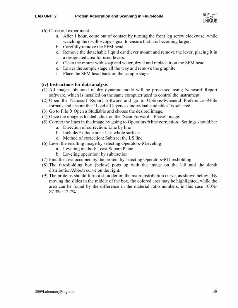
(iv) Instructions for data analysis (1) All images obtained in dry dynamic mode will be processed using Nanosurf Report
software, which is installed on the same computer used to control the instrument. (2) Open the Nanosurf Report software and go to Options�General Preferences�File
formats and ensure that ‘Load all layers as individual studiables’ is selected. (3) Go to File� Open a Studiable and choose the desired image. (4) Once the image is loaded, click on the ‘Scan Forward—Phase’ image. (5) Correct the lines in the image by going to Operators�line correction. Settings should be:
a. Direction of correction: Line by line b. Include/Exclude area: Use whole surface c. Method of correction: Subtract the LS line
(6) Level the resulting image by selecting Operators�Leveling a. Leveling method: Least Square Plane b. Leveling operation: by subtraction
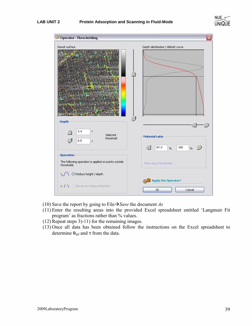
(7) Find the area occupied by the protein by selecting Operators�Thresholding (8) The thresholding box (below) pops up with the image on the left and the depth
distribution/Abbott curve on the right. (9) The proteins should form a shoulder on the main distribution curve, as shown below. By
moving the slides in the middle of the box, the colored area may be highlighted, while the area can be found by the difference in the material ratio numbers, in this case 100%-87.3%=12.7%.
LAB UNIT 2 Protein Adsorption and Scanning in Fluid-Mode
2009LaboratoryProgram 39
(10) Save the report by going to File�Save the document As (11) Enter the resulting areas into the provided Excel spreadsheet entitled ‘Langmuir Fit
program’ as fractions rather than % values. (12) Repeat steps 3)-11) for the remaining images. (13) Once all data has been obtained follow the instructions on the Excel spreadsheet to
determine θinf and τ from the data.

LAB UNIT 2 Protein Adsorption and Scanning in Fluid-Mode
2009LaboratoryProgram 40
4. Background: Fibrinogen’s Role in Biomaterial Response and Protein-Solid Interactions
Table of Contents:
Brief Overview on Blood Clotting ............................................................................ 40 Fibrinogen Structure and Functioning Mechanism................................................... 42 Bio-Response toward Implant Devices and Foreign Bodies..................................... 43 Implant Material Design............................................................................................ 44 Characterization of Adsorption Processes................................................................. 47 Artificial Nose or Biosensor...................................................................................... 50 References ................................................................................................................. 51
Brief Overview on Blood Clotting Medical implants used today can incur thousands of dollars in cost to the patient and often
require invasive methods of maintenance and eventual replacement (see Fig. 1) to correct unintended physiological responses by the body (bio-response). While many of these complications stem from the implant design, broad limitations exist in designing proper material interfaces that can coexist the dynamic environment of the body and its complex biochemical response to foreign surfaces. Therefore, the design of proper biomaterials requires a fundamental understanding of the bio-response mechanism from the body and its ultimate effects at the interface of the material surface.
To understand the body’s response to implanted materials, it is insightful to first study how the body responds to normal internal and external wounds (lacerations), as well as imperfections in everyday functional tissues via blood clotting. The formation of a blood clot is the result of a
Figure 1. Prosthetic carbon-based mechanical heart valve, (left) before implantation, (right) after implantation rejected by the body. Courtesy of T. Horbert (University of Washington)
LAB UNIT 2 Protein Adsorption and Scanning in Fluid-Mode
2009LaboratoryProgram 41
concerted interplay between various blood components, such as the platelets, or thrombocytes, The platelets are cells in the blood that are involved in the cellular mechanisms of the primary blood clotting process, the hemostasis.
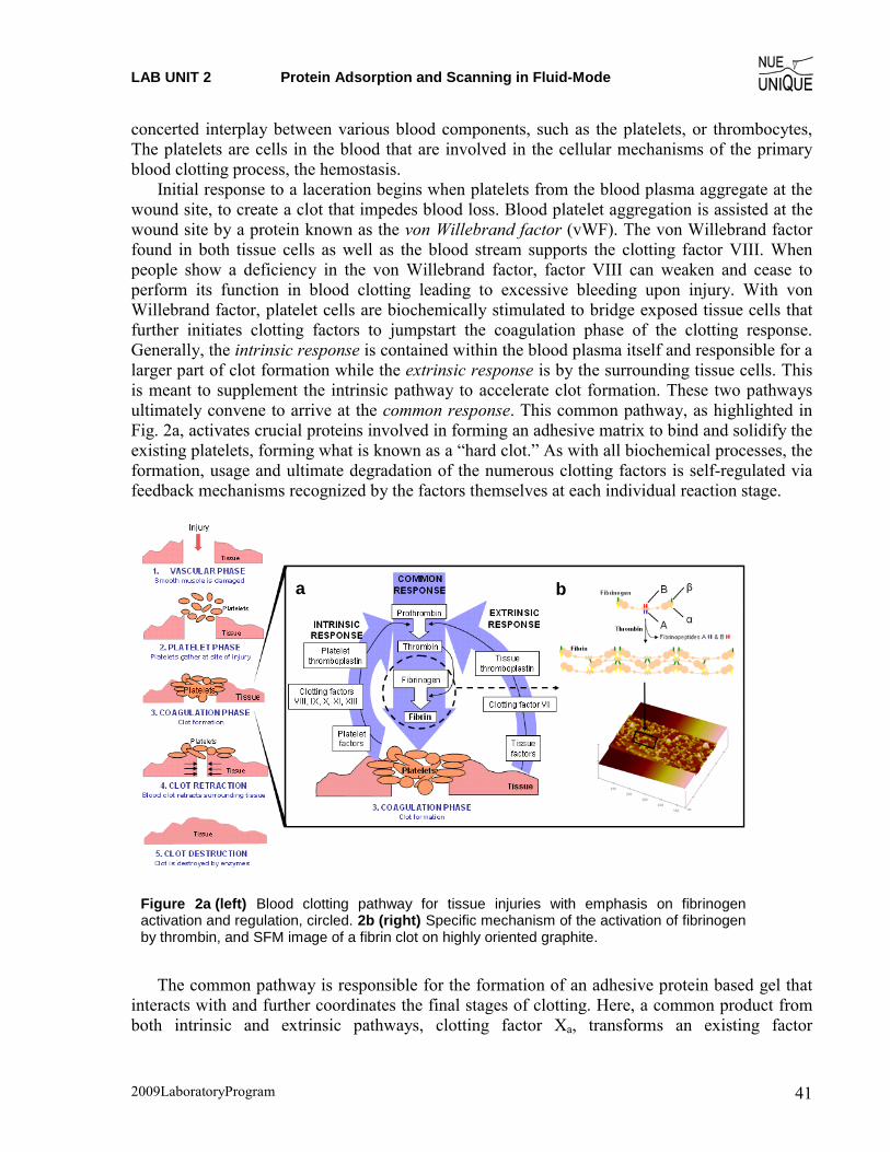
Initial response to a laceration begins when platelets from the blood plasma aggregate at the wound site, to create a clot that impedes blood loss. Blood platelet aggregation is assisted at the wound site by a protein known as the von Willebrand factor (vWF). The von Willebrand factor found in both tissue cells as well as the blood stream supports the clotting factor VIII. When people show a deficiency in the von Willebrand factor, factor VIII can weaken and cease to perform its function in blood clotting leading to excessive bleeding upon injury. With von Willebrand factor, platelet cells are biochemically stimulated to bridge exposed tissue cells that further initiates clotting factors to jumpstart the coagulation phase of the clotting response. Generally, the intrinsic response is contained within the blood plasma itself and responsible for a larger part of clot formation while the extrinsic response is by the surrounding tissue cells. This is meant to supplement the intrinsic pathway to accelerate clot formation. These two pathways ultimately convene to arrive at the common response. This common pathway, as highlighted in Fig. 2a, activates crucial proteins involved in forming an adhesive matrix to bind and solidify the existing platelets, forming what is known as a “hard clot.” As with all biochemical processes, the formation, usage and ultimate degradation of the numerous clotting factors is self-regulated via feedback mechanisms recognized by the factors themselves at each individual reaction stage.
The common pathway is responsible for the formation of an adhesive protein based gel that interacts with and further coordinates the final stages of clotting. Here, a common product from both intrinsic and extrinsic pathways, clotting factor Xa, transforms an existing factor
Figure 2a (left) Blood clotting pathway for tissue injuries with emphasis on fibrinogen activation and regulation, circled. 2b (right) Specific mechanism of the activation of fibrinogen by thrombin, and SFM image of a fibrin clot on highly oriented graphite.
a b

LAB UNIT 2 Protein Adsorption and Scanning in Fluid-Mode
2009LaboratoryProgram 42
‘prothrombin’ to its active form ‘thrombin’. This active form then proceeds to activate another factor, fibrinogen, by breaking specific intramolecular connections in a process known as cleavage. Active fibrinogen, referred to as ‘fibrin monomer’, is responsible for polymerizing with itself at the previously cleaved sites to rapidly form an adhesive gel to support the surrounding platelet aggregation in what is known as a ‘soft clot’. Thus, the common pathway and resulting fibrin polymer is the product of both the intrinsic and extrinsic pathways and the main driving force in the clotting cascade’s coagulation phase. The mechanism of fibrin polymer formation is shown in Figure 2b, which also provides a visualization of the fibrin matrix on a model implant surface (graphitic carbon) by scanning force microscopy (SFM).
Fibrinogen Structure and Functioning Mechanism Fibrinogen in its inactive form is 340 kD (~47.5 nm) in size and exists as a covalently bound
two part molecule (known as a “dimer”) associated through three disulfide bridges, as shown in Fig. 3. It is comprised of three intertwined strands of amino acids shown in Fig. 3b as the A, B, and C strands. These strands associate with each other to form several functional domains, including the terminal sticky α, β, and γ domains (shown as tangled lines in Fig. 3b) of the protein as well as the rigid spacer linking the two portions of the dimer together. From the center, strands A and B contain short sequences of amino acids which together form the thrombin cleavage site, shown as stemmed circles in Fig. 3b. After the short sequences (known as ‘fibrinopeptides’) are cleaved off, the newly vacant sites (pathway shown in Fig. 2b) are now free to interact specifically with the sticky α and β domains from adjacent fibrin monomers for polymerization and the formation of a ‘soft clot’. Further, polysaccharides contained within the terminal sticky ends of fibrin (shown as black hexagons in Fig. 3b) help provide an even stronger fibrin polymer through a process called cross-linking (off-axis bonding) to ultimately form a ‘hard clot’ via a factor known as XIIIa. These domains of fibrin are spaced ~16 nm from the center domain via a structured triple-helix spacer domain, where the three strands are intertwined to give fibrinogen and the resulting clot a rigid structure.
The last domain, the γ-sticky end also plays a crucial role (as seen in Fig. 4a) in interacting with platelet cell surface receptors to ultimately incorporate the existing platelets into the fibrin clot. Typically, both inactive and active forms of fibrinogen can mediate adhesion via γ-domain interaction with platelet surface-bound factors known as GPIIb/IIIa. When these surface receptors are bound, platelets switch from inactive to active form and begin to secrete cofactors (a factor designed to work with another factor) and signaling proteins (including fibrinogen and vWF) which act as positive feedback agents to further promote clot formation. As covered in the next section, this interaction plays a crucial role in implant rejection due to the lack of need for an active form of fibrinogen to initiate a clotting cascade.

LAB UNIT 2 Protein Adsorption and Scanning in Fluid-Mode
2009LaboratoryProgram 43
Bio-Response toward Implant Devices and Foreign Bodies Many of the same factors play a role in the identification and isolation of foreign material
surfaces in the body, which leads to ‘rejections’. One major difference, however, is the lack of vWF or other existing extrinsic pathways to supplement or jumpstart the bio-response cascade as
Figure 3. a (top) Crystal structure of fibrinogen, showing the triple helix structure of linker regions and b (bottom) color corresponding diagram of three separate protein strands A,B,C and their association with each other via disulfide bridges.
Figure 4a. Role of fibrinogen as a recruiter and adhesive of platelets.
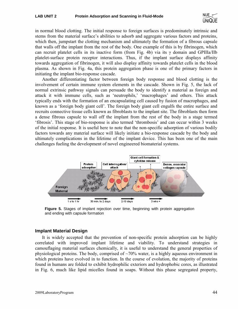
Figure 4b. Structure of a clot on a foreign surface, showing initial layer of adsorbed proteins with extended coating of coordinated platelets via fibrinogen.
LAB UNIT 2 Protein Adsorption and Scanning in Fluid-Mode
2009LaboratoryProgram 44
in normal blood clotting. The initial response to foreign surfaces is predominately intrinsic and stems from the material surface’s abilities to adsorb and aggregate various factors and proteins, which then, jumpstart the clotting mechanism and ultimately the formation of a fibrous capsule that walls off the implant from the rest of the body. One example of this is by fibrinogen, which can recruit platelet cells in its inactive form (from Fig. 4b) via its γ domain and GPIIIa/IIb platelet-surface protein receptor interactions. Thus, if the implant surface displays affinity towards aggregation of fibrinogen, it will also display affinity towards platelet cells in the blood plasma. As shown in Fig. 4a, this protein aggregation phase is one of the primary factors in initiating the implant bio-response cascade.
Another differentiating factor between foreign body response and blood clotting is the involvement of certain immune system elements in the cascade. Shown in Fig. 5, the lack of normal extrinsic pathway signals can persuade the body to identify a material as foreign and attack it with immune cells, such as ‘neutrophils,’ ‘macrophages’ and others. This attack typically ends with the formation of an encapsulating cell caused by fusion of macrophages, and known as a ‘foreign body giant cell’. The foreign body giant cell engulfs the entire surface and recruits connective tissue cells known as fibroblasts to the implant site. The fibroblasts then form a dense fibrous capsule to wall off the implant from the rest of the body in a stage termed ‘fibrosis’. This stage of bio-response is also termed ‘thrombosis’ and can occur within 3 weeks of the initial response. It is useful here to note that the non-specific adsorption of various bodily factors towards any material surface will likely initiate a bio-response cascade by the body and ultimately complications in the lifetime of the implant device. This has been one of the main challenges fueling the development of novel engineered biomaterial systems.
Implant Material Design It is widely accepted that the prevention of non-specific protein adsorption can be highly
correlated with improved implant lifetime and viability. To understand strategies in camouflaging material surfaces chemically, it is useful to understand the general properties of physiological proteins. The body, comprised of ~70% water, is a highly aqueous environment in which proteins have evolved in to function. In the course of evolution, the majority of proteins found in humans are folded to exhibit hydrophilic exteriors and hydrophobic cores, as illustrated in Fig. 6, much like lipid micelles found in soaps. Without this phase segregated property,
Figure 5. Stages of implant rejection over time, beginning with protein aggregation and ending with capsule formation
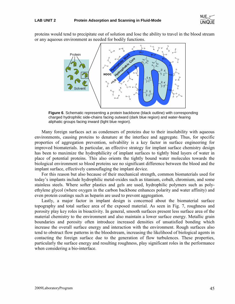
LAB UNIT 2 Protein Adsorption and Scanning in Fluid-Mode
2009LaboratoryProgram 45
proteins would tend to precipitate out of solution and lose the ability to travel in the blood stream or any aqueous environment as needed for bodily functions.
Figure 6. Schematic representing a protein backbone (black outline) with corresponding charged hydrophilic side-chains facing outward (dark blue region) and water-fearing aliphatic groups facing inward (light blue region).
Many foreign surfaces act as condensers of proteins due to their insolubility with aqueous environments, causing proteins to denature at the interface and aggregate. Thus, for specific properties of aggregation prevention, solvability is a key factor in surface engineering for improved biomaterials. In particular, an effective strategy for implant surface chemistry design has been to maximize the hydrophilicity of implant surfaces to tightly bind layers of water in place of potential proteins. This also orients the tightly bound water molecules towards the biological environment so blood proteins see no significant difference between the blood and the implant surface, effectively camouflaging the implant device.
For this reason but also because of their mechanical strength, common biomaterials used for today’s implants include hydrophilic metal-oxides such as titanium, cobalt, chromium, and some stainless steels. Where softer plastics and gels are used, hydrophilic polymers such as poly-ethylene glycol (where oxygen in the carbon backbone enhances polarity and water affinity) and even protein coatings such as heparin are used to prevent aggregation.
Lastly, a major factor in implant design is concerned about the biomaterial surface topography and total surface area of the exposed material. As seen in Fig. 7, roughness and porosity play key roles in bioactivity. In general, smooth surfaces present less surface area of the material chemistry to the environment and also maintain a lower surface energy. Metallic grain boundaries and porosity often introduce increased densities of unsatisfied bonding which increase the overall surface energy and interaction with the environment. Rough surfaces also tend to obstruct flow patterns in the bloodstream, increasing the likelihood of biological agents in contacting the foreign surface due to the generation of flow turbulences. These properties, particularly the surface energy and resulting roughness, play significant roles in the performance when considering a bio-interface.
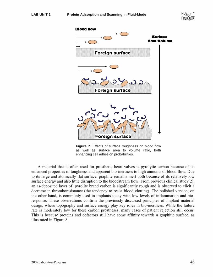
LAB UNIT 2 Protein Adsorption and Scanning in Fluid-Mode
2009LaboratoryProgram 46
A material that is often used for prosthetic heart valves is pyrolytic carbon because of its enhanced properties of toughness and apparent bio-inertness to high amounts of blood flow. Due to its large and atomically flat surface, graphite remains inert both because of its relatively low surface energy and also little disruption to the bloodstream flow. From previous clinical study[2], an as-deposited layer of pyrolite brand carbon is significantly rough and is observed to elicit a decrease in thromboresistance (the tendency to resist blood clotting). The polished version, on the other hand, is commonly used in implants today with low levels of inflammation and bio-response. These observations confirm the previously discussed principles of implant material design, where topography and surface energy play key roles in bio-inertness. While the failure rate is moderately low for these carbon prostheses, many cases of patient rejection still occur. This is because proteins and cofactors still have some affinity towards a graphitic surface, as illustrated in Figure 8.
Figure 7. Effects of surface roughness on blood flow as well as surface area to volume ratio, both enhancing cell adhesion probabilities.
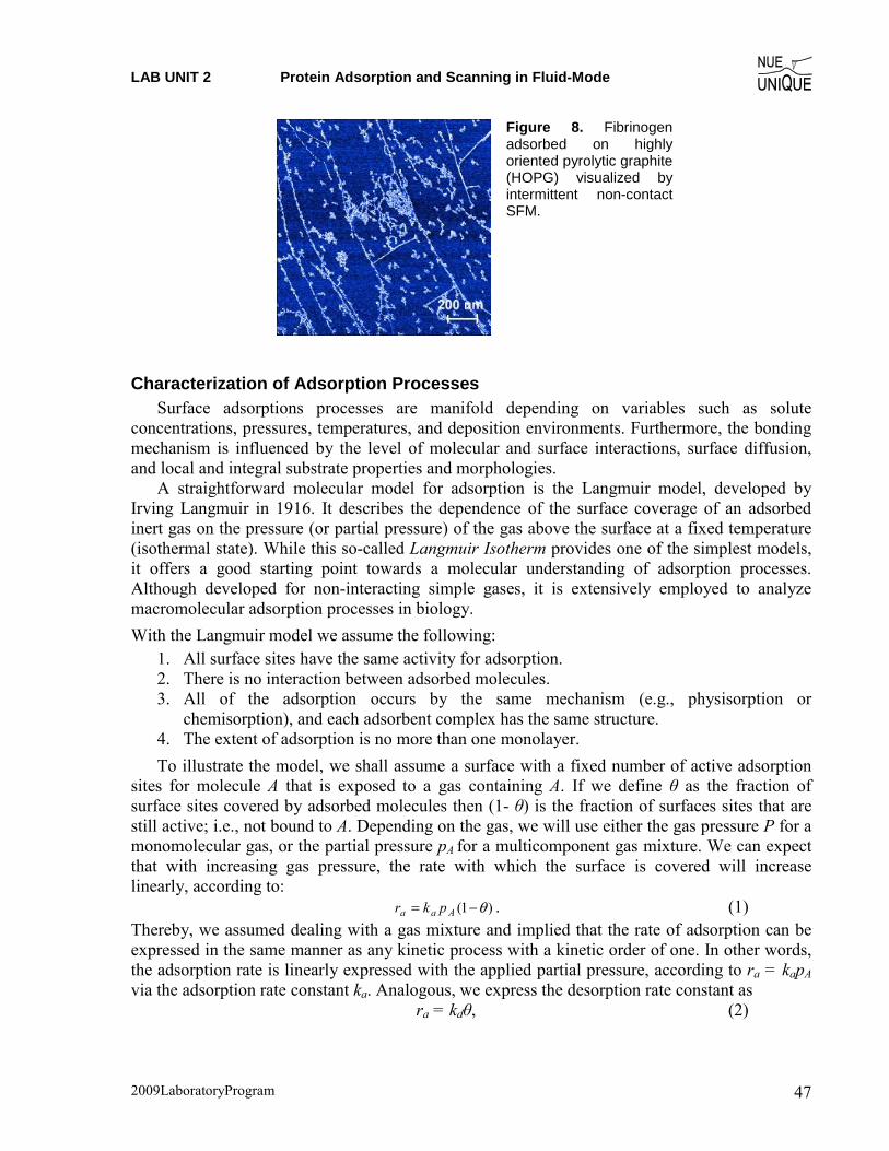
LAB UNIT 2 Protein Adsorption and Scanning in Fluid-Mode
2009LaboratoryProgram 47
Figure 8. Fibrinogen adsorbed on highly oriented pyrolytic graphite (HOPG) visualized by intermittent non-contact SFM.
Characterization of Adsorption Processes Surface adsorptions processes are manifold depending on variables such as solute
concentrations, pressures, temperatures, and deposition environments. Furthermore, the bonding mechanism is influenced by the level of molecular and surface interactions, surface diffusion, and local and integral substrate properties and morphologies.
A straightforward molecular model for adsorption is the Langmuir model, developed by Irving Langmuir in 1916. It describes the dependence of the surface coverage of an adsorbed inert gas on the pressure (or partial pressure) of the gas above the surface at a fixed temperature (isothermal state). While this so-called Langmuir Isotherm provides one of the simplest models, it offers a good starting point towards a molecular understanding of adsorption processes. Although developed for non-interacting simple gases, it is extensively employed to analyze macromolecular adsorption processes in biology.
With the Langmuir model we assume the following:
1. All surface sites have the same activity for adsorption. 2. There is no interaction between adsorbed molecules. 3. All of the adsorption occurs by the same mechanism (e.g., physisorption or
chemisorption), and each adsorbent complex has the same structure. 4. The extent of adsorption is no more than one monolayer.
To illustrate the model, we shall assume a surface with a fixed number of active adsorption sites for molecule A that is exposed to a gas containing A. If we define θ as the fraction of surface sites covered by adsorbed molecules then (1- θ) is the fraction of surfaces sites that are still active; i.e., not bound to A. Depending on the gas, we will use either the gas pressure P for a monomolecular gas, or the partial pressure pA for a multicomponent gas mixture. We can expect that with increasing gas pressure, the rate with which the surface is covered will increase linearly, according to: )1( θ−= Aaa pkr . (1) Thereby, we assumed dealing with a gas mixture and implied that the rate of adsorption can be expressed in the same manner as any kinetic process with a kinetic order of one. In other words, the adsorption rate is linearly expressed with the applied partial pressure, according to ra = kapA via the adsorption rate constant ka. Analogous, we express the desorption rate constant as ra = kdθ, (2)
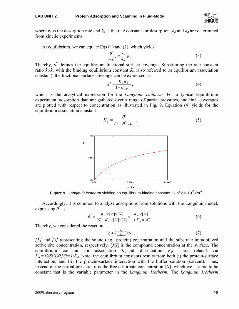
LAB UNIT 2 Protein Adsorption and Scanning in Fluid-Mode
2009LaboratoryProgram 48
where ra is the desorption rate and kd is the rate constant for desorption. ka and kd are determined from kinetic experiments
At equilibrium, we can equate Eqs (1) and (2), which yields
Ad
a pkk
=− *
*
1 θθ . (3)
Thereby, θ* defines the equilibrium fractional surface coverage. Substituting the rate constant ratio ka/kd with the binding equilibrium constant Ka (also referred to as equilibrium association constant), the fractional surface coverage can be expressed as
Aa
Aa
pKpK
+=
1*θ , (4)
which is the analytical expression for the Langmuir Isotherm. For a typical equilibrium experiment, adsorption data are gathered over a range of partial pressures, and final coverages are plotted with respect to concentration as illustrated in Fig. 9. Equation (4) yields for the equilibrium association constant
A
*
*
a p)(K
θθ
−=
1. (5)
Figure 9. Langmuir Isotherm yielding an equilibrium binding constant Ka of 2 × 10⁻⁵ Pa-1. Accordingly, it is common to analyze adsorptions from solutions with the Langmuir model,
expressing θ* as:
][1
][][][][
][][*
XKXK
SXKSSXK
a
a
a
a
×+×
=××+
××=θ . (6)
Thereby, we considered the reaction XSSX
aK
dK⎯⎯ →⎯
⎯⎯ ⎯←+ , (7)
[X] and [S] representing the solute (e.g., protein) concentration and the substrate immobilized active site concentration, respectively. [XS] is the compound concentration at the surface. The equilibrium constant for association Ka and dissociation Kd are related via Ka = [XS]/[X][S]=1/Kd. Note, the equilibrium constants results from both (i) the protein-surface interaction, and (ii) the protein-surface interaction with the buffer solution (solvent). Thus, instead of the partial pressure, it is the free adsorbate concentration [X], which we assume to be constant that is the variable parameter in the Langmuir Isotherm. The Langmuir Isotherm
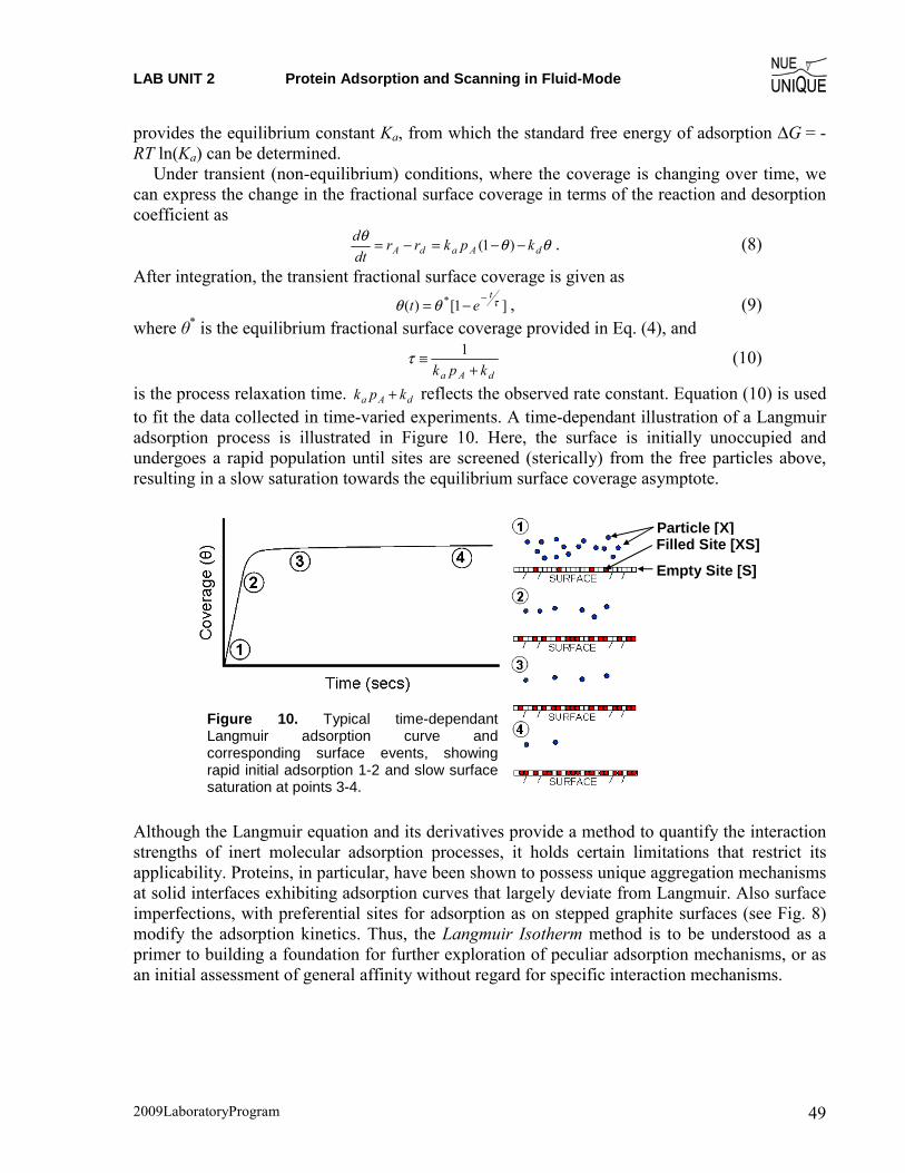
LAB UNIT 2 Protein Adsorption and Scanning in Fluid-Mode
2009LaboratoryProgram 49
provides the equilibrium constant Ka, from which the standard free energy of adsorption ΔG = -RT ln(Ka) can be determined.
Under transient (non-equilibrium) conditions, where the coverage is changing over time, we can express the change in the fractional surface coverage in terms of the reaction and desorption coefficient as
θθθdAadA kpkrr
dtd −−=−= )1( . (8)
After integration, the transient fractional surface coverage is given as ]1[)( * τθθ
tet −−= , (9)
where θ* is the equilibrium fractional surface coverage provided in Eq. (4), and
dAa kpk +
≡ 1τ (10)
is the process relaxation time. dAa kpk + reflects the observed rate constant. Equation (10) is used to fit the data collected in time-varied experiments. A time-dependant illustration of a Langmuir adsorption process is illustrated in Figure 10. Here, the surface is initially unoccupied and undergoes a rapid population until sites are screened (sterically) from the free particles above, resulting in a slow saturation towards the equilibrium surface coverage asymptote.
Although the Langmuir equation and its derivatives provide a method to quantify the interaction strengths of inert molecular adsorption processes, it holds certain limitations that restrict its applicability. Proteins, in particular, have been shown to possess unique aggregation mechanisms at solid interfaces exhibiting adsorption curves that largely deviate from Langmuir. Also surface imperfections, with preferential sites for adsorption as on stepped graphite surfaces (see Fig. 8) modify the adsorption kinetics. Thus, the Langmuir Isotherm method is to be understood as a primer to building a foundation for further exploration of peculiar adsorption mechanisms, or as an initial assessment of general affinity without regard for specific interaction mechanisms.
Particle [X]Filled Site [XS]
Empty Site [S]
Figure 10. Typical time-dependant Langmuir adsorption curve and corresponding surface events, showing rapid initial adsorption 1-2 and slow surface saturation at points 3-4.
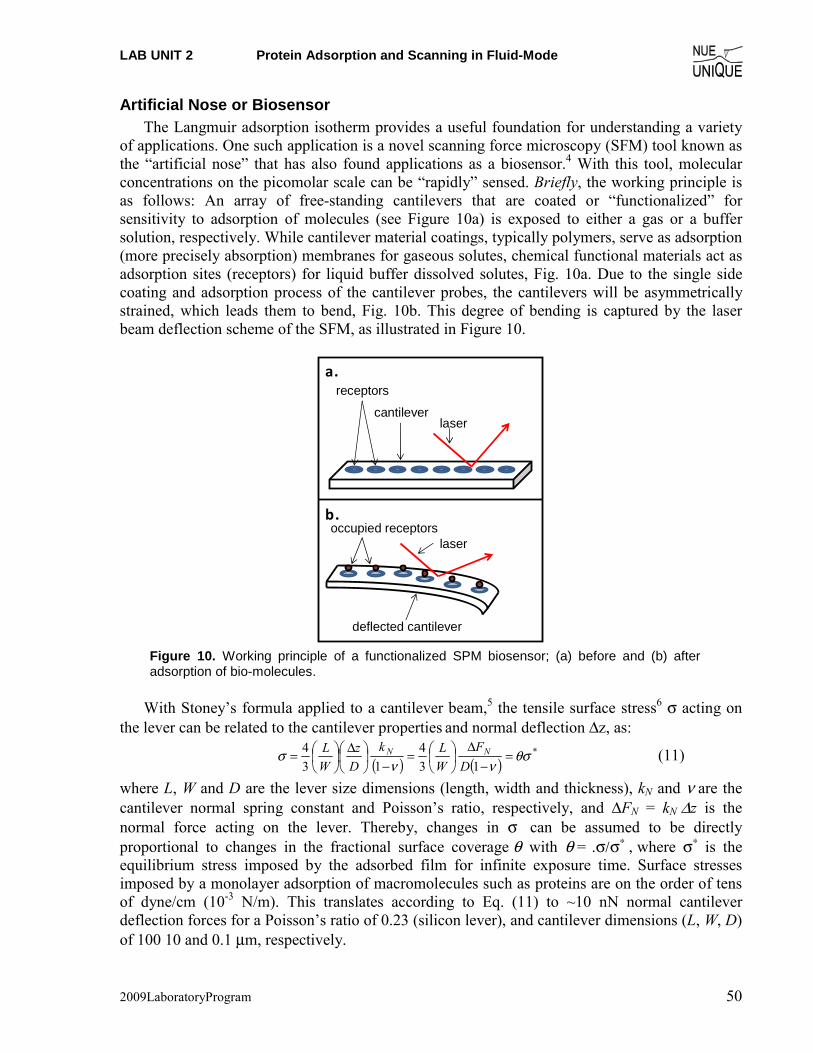
LAB UNIT 2 Protein Adsorption and Scanning in Fluid-Mode
2009LaboratoryProgram 50
Artificial Nose or Biosensor The Langmuir adsorption isotherm provides a useful foundation for understanding a variety
of applications. One such application is a novel scanning force microscopy (SFM) tool known as the “artificial nose” that has also found applications as a biosensor.4 With this tool, molecular concentrations on the picomolar scale can be “rapidly” sensed. Briefly, the working principle is as follows: An array of free-standing cantilevers that are coated or “functionalized” for sensitivity to adsorption of molecules (see Figure 10a) is exposed to either a gas or a buffer solution, respectively. While cantilever material coatings, typically polymers, serve as adsorption (more precisely absorption) membranes for gaseous solutes, chemical functional materials act as adsorption sites (receptors) for liquid buffer dissolved solutes, Fig. 10a. Due to the single side coating and adsorption process of the cantilever probes, the cantilevers will be asymmetrically strained, which leads them to bend, Fig. 10b. This degree of bending is captured by the laser beam deflection scheme of the SFM, as illustrated in Figure 10.
receptors
occupied receptors
cantileverlaser
laser
deflected cantilever
a.
b.
Figure 10. Working principle of a functionalized SPM biosensor; (a) before and (b) after adsorption of bio-molecules.
With Stoney’s formula applied to a cantilever beam,5 the tensile surface stress6 σ acting on
the lever can be related to the cantilever properties and normal deflection Δz, as:
( ) ( )*
134
134 θσ
ννσ =
−Δ
⎟⎠
⎞⎜⎝
⎛=−
⎟⎠
⎞⎜⎝
⎛ Δ⎟⎠
⎞⎜⎝
⎛=D
FWLk
Dz
WL NN (11)
where L, W and D are the lever size dimensions (length, width and thickness), kN and ν are the cantilever normal spring constant and Poisson’s ratio, respectively, and ΔFN = kN Δz is the normal force acting on the lever. Thereby, changes in σ can be assumed to be directly proportional to changes in the fractional surface coverage θ with θ = .σ/σ∗
, where σ∗ is the equilibrium stress imposed by the adsorbed film for infinite exposure time. Surface stresses imposed by a monolayer adsorption of macromolecules such as proteins are on the order of tens of dyne/cm (10-3 N/m). This translates according to Eq. (11) to ~10 nN normal cantilever deflection forces for a Poisson’s ratio of 0.23 (silicon lever), and cantilever dimensions (L, W, D) of 100 10 and 0.1 μm, respectively.

LAB UNIT 2 Protein Adsorption and Scanning in Fluid-Mode
2009LaboratoryProgram 51
References 1. Gettens, R.T.T., Z. Bai and J.L. Gilbert, Quantification of the kinetics and thermodynamics of
protein adsorption using atomic force microscopy, Journal of Biomedical Materials Research, Part A, 2005. 72A(3): p. 246-257.
2. Bokros, J.C., L.D. LaGrange and F.J. Schoen, Control of structure of carbon for use in bioengineering, Chemistry and Physics of Carbon, 1973. 9: p. 103-71.
3. Sit, P.S. and R.E. Marchant, Surface-dependent differences in fibrin assembly. visualized by atomic force microscopy, Surface Science, 2001. 491(3): p. 421-432.
4. Fritz, J.; Baller, M.K.; Lang, H.P.; Rothuizen, H.; Vettiger, P.; Meyer, E.; Güntherodt, H.-J.; Gerber, C.; Gimzewski, J.K.: Translating biomolecular recognition into nanomechanics, Science, 2000, 288 p. 316-318.
5. Nanoscience – Friction and Rheology on the Nanometer Scale, Meyer, E., Overney, R.M., Dransfeld, K., Gyalog, T., World Scientific (New Jersey) 1998, p. 186.
6. For an adsorbed film of thickness tF, the surface tensile stress σ [N/m] is related to the stress in the adsorbed film along the cantilever beam σF [Pa = N/m2] via σ = σF / tF.

LAB UNIT 2 Protein Adsorption and Scanning in Fluid-Mode
2009LaboratoryProgram 52
5. Appendix Simple Harmonic Motion
Having covered the fundamentals of the materials in question in this lab we now move to the operation of the scanning probe microscope itself. For this lab we will be using ‘dynamic’ or ‘AC’ mode imaging, to prevent the tip from damaging the protein as it scans. We will use this method both in air and in liquid (phosphate buffer solution, PBS) to measure protein adsorption behavior in situ (PBS) and ex situ (air).
The SPM tip sits at the end of a long, flexible cantilever. This cantilever is flexible and behaves like a spring: if the tip is pushed in one direction the cantilever exerts a force in the opposite direction in an attempt to restore the tip to its original position. Since we are going to be examining the motion of the tip in more detail, we first define some parameters:
z(t) position of the tip as a function of time F force exerted on the tip m mass of the tip k effective spring constant of the cantilever
Remember that the velocity v(t) and acceleration a(t) of the tip are related to its position z(t) through the following derivatives:
dtdztv =)( 2
2
)(dt
zddtdvta == (1a,b)
Newton’s third law (F = ma) relates the forces on the tip to its motion. We already mentioned that the cantilever behaves much like a spring, and will we approximate the restoring force using Hooke’s law relating spring constants and restoring forces (F = –kz). Combining these two equations gives us the following equation of motion:
kz
dtzdm
kzmaF
−=
−==
2
2 (2a, b)
The tip and cantilever are real materials moving through air, so the motion is also damped by both air friction (or water friction in fluid mode) and by losses in the spring. These losses are both approximately proportional to the velocity and so we modify our equation of motion with a “drag force” or damping term –bv:
dtdzbkz
dtzdm
bvkzmaF
−−=
−−==
2
2 (3a, b)
Rearranging a bit, we can write this as a differential equation describing basic motion of the tip far away from any substrate (and still without any driving force yet either)
LAB UNIT 2 Protein Adsorption and Scanning in Fluid-Mode
2009LaboratoryProgram 53
0
0
202
2
2
2
=++
=++
zdtdz
dtzd
kzdtdzb
dtzdm
ωβ (4a,b)
where ω0
2≡ k/m and β ≡ b/m. ω0 is the natural frequency of the cantilever.
Most non-contact/intermittent contact SPM is performed while applying a sinusoidally oscillating drive force on the tip, so we must also add the driving force to our equation of motion:
tDzdtdz
dtzd ωωβ cos2
02
2
=++ (5)
This equation may look familiar. It is the classic equation for the damped and driven simple harmonic oscillator. The solution to this equation is a steady-state motion of the system should oscillate with the driving force, plus a potential phase shift δ. You can check that the solution has the form: )cos()( δω −= tAtz (6) where:
⎟⎟⎠
⎞⎜⎜⎝
⎛
−= −
220
1tanωω
ωβδ (7)
The amplitude, A, of oscillation is:
22222
0 )( βωωω +−= DA (8)
The “resonance frequency” of the oscillator is defined as the driving frequency at which A is maximized. If the damping is small, the amplitude is at a maximum when the driving frequency equals the natural frequency ω0. The amount of damping in a simple harmonic oscillator is commonly characterized by the quality factor, Q. Q is defined as the resonance frequency divided by β, and is a measure of the total energy stored in the oscillator divided by the energy lost per period of oscillation. For systems that are only weakly damped (like an SFM tip vibrating in air), a practical method of determining Q is to divide the resonance frequency by the width of the resonance peak (where the width is taken at the points where the amplitude is equal to 707.02/1 ≈ of the maximum). In the case of liquid imaging, the resonance frequency changes substantially as the system is not only further damped, but also must move a larger mass (including liquid) during the oscillation process.
AC-Mode Imaging In a common form of topography imaging, called intermittent-contact mode (or a variation
called “Tapping Mode™”, or “dynamic mode” by some manufacturers), the SFM is driven at a
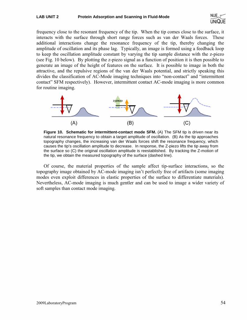
LAB UNIT 2 Protein Adsorption and Scanning in Fluid-Mode
2009LaboratoryProgram 54
frequency close to the resonant frequency of the tip. When the tip comes close to the surface, it interacts with the surface through short range forces such as van der Waals forces. These additional interactions change the resonance frequency of the tip, thereby changing the amplitude of oscillation and its phase lag. Typically, an image is formed using a feedback loop to keep the oscillation amplitude constant by varying the tip sample distance with the z-piezo (see Fig. 10 below). By plotting the z-piezo signal as a function of position it is then possible to generate an image of the height of features on the surface. It is possible to image in both the attractive, and the repulsive regions of the van der Waals potential, and strictly speaking this divides the classification of AC-Mode imaging techniques into “non-contact” and “intermittent contact” SFM respectively). However, intermittent contact AC-mode imaging is more common for routine imaging.
Figure 10. Schematic for intermittent-contact mode SFM. (A) The SFM tip is driven near its natural resonance frequency to obtain a target amplitude of oscillation. (B) As the tip approaches topography changes, the increasing van der Waals forces shift the resonance frequency, which causes the tip’s oscillation amplitude to decrease. In response, the Z-piezo lifts the tip away from the surface so (C) the original oscillation amplitude is reestablished. By tracking the Z-motion of the tip, we obtain the measured topography of the surface (dashed line).
Of course, the material properties of the sample affect tip-surface interactions, so the
topography image obtained by AC-mode imaging isn’t perfectly free of artifacts (some imaging modes even exploit differences in elastic properties of the surface to differentiate materials). Nevertheless, AC-mode imaging is much gentler and can be used to image a wider variety of soft samples than contact mode imaging.
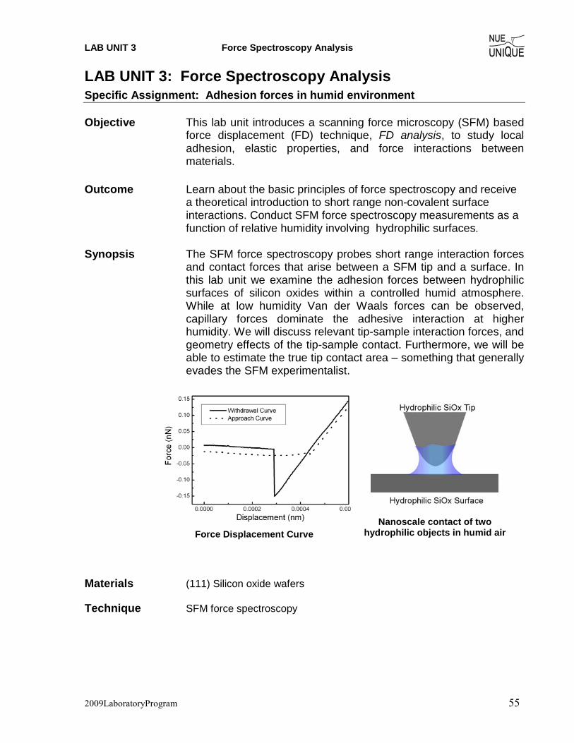
LAB UNIT 3 Force Spectroscopy Analysis
2009LaboratoryProgram 55
LAB UNIT 3: Force Spectroscopy Analysis Specific Assignment: Adhesion forces in humid environment Objective This lab unit introduces a scanning force microscopy (SFM) based
force displacement (FD) technique, FD analysis, to study local adhesion, elastic properties, and force interactions between materials.
Outcome Learn about the basic principles of force spectroscopy and receive
a theoretical introduction to short range non-covalent surface interactions. Conduct SFM force spectroscopy measurements as a function of relative humidity involving hydrophilic surfaces.
Synopsis The SFM force spectroscopy probes short range interaction forces
and contact forces that arise between a SFM tip and a surface. In this lab unit we examine the adhesion forces between hydrophilic surfaces of silicon oxides within a controlled humid atmosphere. While at low humidity Van der Waals forces can be observed, capillary forces dominate the adhesive interaction at higher humidity. We will discuss relevant tip-sample interaction forces, and geometry effects of the tip-sample contact. Furthermore, we will be able to estimate the true tip contact area – something that generally evades the SFM experimentalist.
Force Displacement Curve
Nanoscale contact of two hydrophilic objects in humid air
Materials (111) Silicon oxide wafers Technique SFM force spectroscopy

LAB UNIT 3 Force Spectroscopy Analysis
2009LaboratoryProgram 56
Table of Contents 1. Assignment................................................................................................... 57 2. Quiz – Preparation for the Experiment....................................................... 58
Theoretical Questions................................................................................................ 58 Prelab Quiz ................................................................................................................ 58
3. Experimental Assignment ........................................................................... 60 Goal ........................................................................................................................... 60 Safety......................................................................................................................... 61 Instrumental Setup..................................................................................................... 61 Materials.................................................................................................................... 61 Experimental Procedure ............................................................................................ 61
4. Background: Non-Covalent Short Range Interactions ................................. and Capillary Forces................................................................................ 67
Motivation ................................................................................................................. 67 Short Range Interactions and Surface Forces............................................................ 67 Van der Waals Interactions for Point Interactions .................................................... 69 Surface Forces ........................................................................................................... 69 Hamaker Constant ..................................................................................................... 71 Van der Waals Retardation Effects ........................................................................... 72 Adhesion and Surface Energies................................................................................. 72 Cutoff Distance for Van der Waals Calculations ...................................................... 73 Capillary Forces due to Vapor Condensation ........................................................... 74 Critical Humidity for Capillary Neck Formation ...................................................... 75 Estimation of the Tip Radius Utilizing the Capillary Effects ................................... 76 Modification of Hydrophobicity (Wettability).......................................................... 78 Force Displacement Curves ...................................................................................... 79 References ................................................................................................................. 80 Recommended Reading............................................................................................. 80
5. Appendix....................................................................................................... 81 Tool for Sigmoidal Data Fit ...................................................................................... 81 Tool for Hamaker Constant Calculation (provided in Excel Toolbox)..................... 81
LAB UNIT 3 Force Spectroscopy Analysis
2009LaboratoryProgram 57
1. Assignment The assignment is to experimentally determine the effect of humidity on adhesion forces for hydrophilic surfaces and to employ the theories and background information to discuss the experimental results. The steps are outlined here:
1. Familiarize yourself with the background information provided in Section 4. 2. Test your background knowledge with the provided Quiz in Section 2. 3. Conduct the adhesion-humidity experiments in Section 3. Follow the step-by-step
experimental procedure. 4. Analyze your data as described in Section 3 5. Finally, provide a report with the following information:
(i) Results section: In this section you show your data and discuss instrumental details (i.e., limitations) and the quality of your data (error analysis).
(ii) Discussion section: In this section you discuss and analyze your data in the light of the provided background information.
It is also appropriate to discuss sections (i) and (ii) together. (iii) Summary: Here you summarize your findings and provide comments on how your
results would affect any future AFM work you may do. The report is evaluated based on the quality of the discussion and the integration of your experimental data and the provided theory. You are encouraged to discuss results that are unexpected. It is important to include discussions on the causes for discrepancies and inconsistencies in the data.
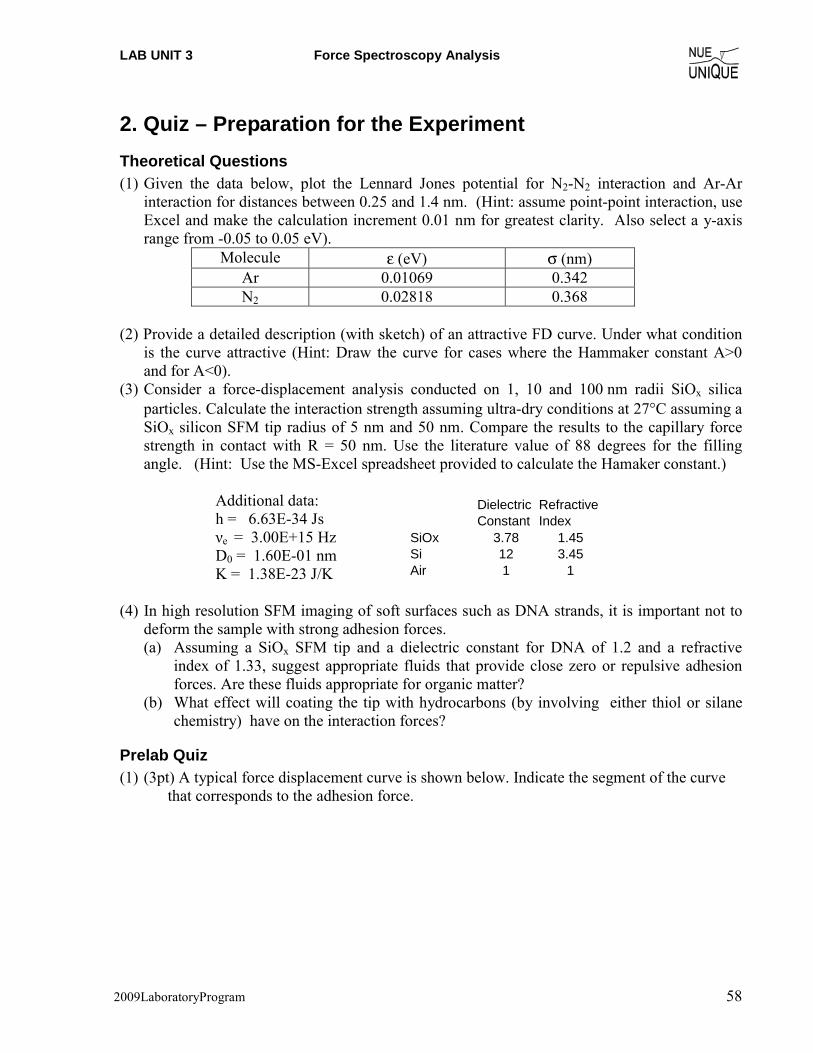
LAB UNIT 3 Force Spectroscopy Analysis
2009LaboratoryProgram 58
Dielectric Constant
Refractive Index
SiOx 3.78 1.45Si 12 3.45Air 1 1
2. Quiz – Preparation for the Experiment Theoretical Questions (1) Given the data below, plot the Lennard Jones potential for N2-N2 interaction and Ar-Ar
interaction for distances between 0.25 and 1.4 nm. (Hint: assume point-point interaction, use Excel and make the calculation increment 0.01 nm for greatest clarity. Also select a y-axis range from -0.05 to 0.05 eV).
Molecule ε (eV) σ (nm) Ar 0.01069 0.342 N2 0.02818 0.368
(2) Provide a detailed description (with sketch) of an attractive FD curve. Under what condition
is the curve attractive (Hint: Draw the curve for cases where the Hammaker constant A>0 and for A<0).
(3) Consider a force-displacement analysis conducted on 1, 10 and 100 nm radii SiOx silica particles. Calculate the interaction strength assuming ultra-dry conditions at 27°C assuming a SiOx silicon SFM tip radius of 5 nm and 50 nm. Compare the results to the capillary force strength in contact with R = 50 nm. Use the literature value of 88 degrees for the filling angle. (Hint: Use the MS-Excel spreadsheet provided to calculate the Hamaker constant.)
Additional data: h = 6.63E-34 Js νe = 3.00E+15 Hz D0 = 1.60E-01 nm K = 1.38E-23 J/K
(4) In high resolution SFM imaging of soft surfaces such as DNA strands, it is important not to
deform the sample with strong adhesion forces. (a) Assuming a SiOx SFM tip and a dielectric constant for DNA of 1.2 and a refractive
index of 1.33, suggest appropriate fluids that provide close zero or repulsive adhesion forces. Are these fluids appropriate for organic matter?
(b) What effect will coating the tip with hydrocarbons (by involving either thiol or silane chemistry) have on the interaction forces?
Prelab Quiz (1) (3pt) A typical force displacement curve is shown below. Indicate the segment of the curve
that corresponds to the adhesion force.
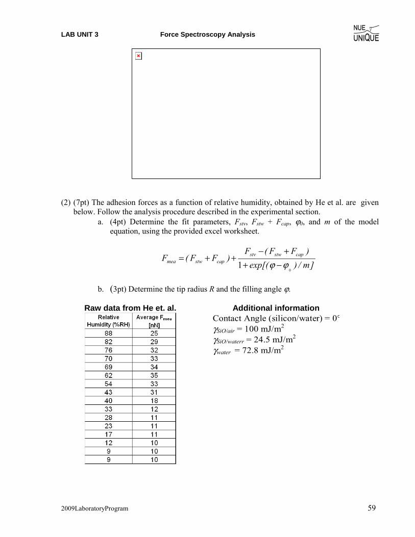
LAB UNIT 3 Force Spectroscopy Analysis
2009LaboratoryProgram 59
(2) (7pt) The adhesion forces as a function of relative humidity, obtained by He et al. are given below. Follow the analysis procedure described in the experimental section.
a. (4pt) Determine the fit parameters, Fstv, Fstw + Fcap, ϕ0, and m of the model equation, using the provided excel worksheet.
]m/)exp[()FF(F
)FF(F capstwstvcapstwmea
01 ϕϕ −+
+−++=
b. (3pt) Determine the tip radius R and the filling angle ϕ.
Raw data from He et. al. Additional information
Contact Angle (silicon/water) = 0°γSiO/air = 100 mJ/m2 γSiO/waterr = 24.5 mJ/m2 γwater = 72.8 mJ/m2
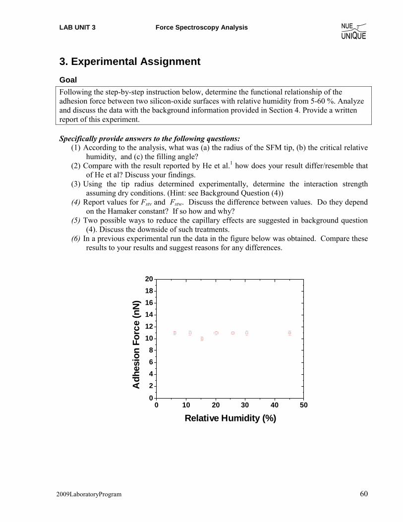
LAB UNIT 3 Force Spectroscopy Analysis
2009LaboratoryProgram 60
3. Experimental Assignment Goal Following the step-by-step instruction below, determine the functional relationship of the adhesion force between two silicon-oxide surfaces with relative humidity from 5-60 %. Analyze and discuss the data with the background information provided in Section 4. Provide a written report of this experiment. Specifically provide answers to the following questions:
(1) According to the analysis, what was (a) the radius of the SFM tip, (b) the critical relative humidity, and (c) the filling angle?
(2) Compare with the result reported by He et al.1 how does your result differ/resemble that of He et al? Discuss your findings.
(3) Using the tip radius determined experimentally, determine the interaction strength assuming dry conditions. (Hint: see Background Question (4))
(4) Report values for Fstv and Fstw. Discuss the difference between values. Do they depend on the Hamaker constant? If so how and why?
(5) Two possible ways to reduce the capillary effects are suggested in background question (4). Discuss the downside of such treatments.
(6) In a previous experimental run the data in the figure below was obtained. Compare these results to your results and suggest reasons for any differences.
0 10 20 30 40 500
2468
101214161820
Adh
esio
n Fo
rce
(nN)
Relative Humidity (%)
LAB UNIT 3 Force Spectroscopy Analysis
2009LaboratoryProgram 61
Safety - Wear safety glasses. - Refer to the General rules in the AFM lab. - The gas cylinder valve should be closed when it is not in use. - Conduct the experiment within the assigned relative humidity range of 5-60% to avoid
electric shortages.
Instrumental Setup - Easy Scan 2 AFM system with contact Mode SFM tip with 0.2 N/m spring constant. - Environmental enclosure and a hygrometer - Nitrogen cylinder and valves - 60 ml beaker within chamber
Materials - Samples: 2 pieces of ~ 1cm2 UV treated (111) silicon wafers securely stored in sealed
Petri dishes till ready for the experiment. - N2 gas - Ultra pure Milli Q water.
Experimental Procedure Read the instructions below carefully and follow them closely. They will provide you with information about (i) preparation of the experiment, (ii) the procedure for force spectroscopy measurements, (iii) the procedure for closing out the experiment, and (iv) on how to conduct the data analysis. (v) A silicon pretreatment (removal of organic contaminants) is provided at the end of this section.
(i) Preparation of the experiment
(1) System Set-up: (This part will be performed with a TA) Follow the start up procedure steps 1 – 8, in the Easy Scan 2 AFM System SOP (Standard Operational Procedure). NOTE: The software leveling step in the SOP is not necessary—skip this step.
a. Place a CONTR cantilever with the spring constant of 0.2 N/ m. b. Positioning procedure should be done with a dummy sample to avoid
contamination. (2) Place a sample piece at the center of the sample holder. Connect the ground wire from the
sample holder to Scan Head. (3) Make sure that the regulator valve and the rotameter are closed. Open the main cylinder
valve. (4) Control the humidity in the glove box. The force-displacement curve will be taken from
low humidity (5%) to high (60%). a. Control the humidity using the N2 gas for the relative humidity between 5% -
ambient humidity of the day (~ 40%). The flow will be adjusted by the rotameter. When conducting the experiment it is generally most efficient to let the humidity increase up to the 15% measurement with the AFM containment in place. For
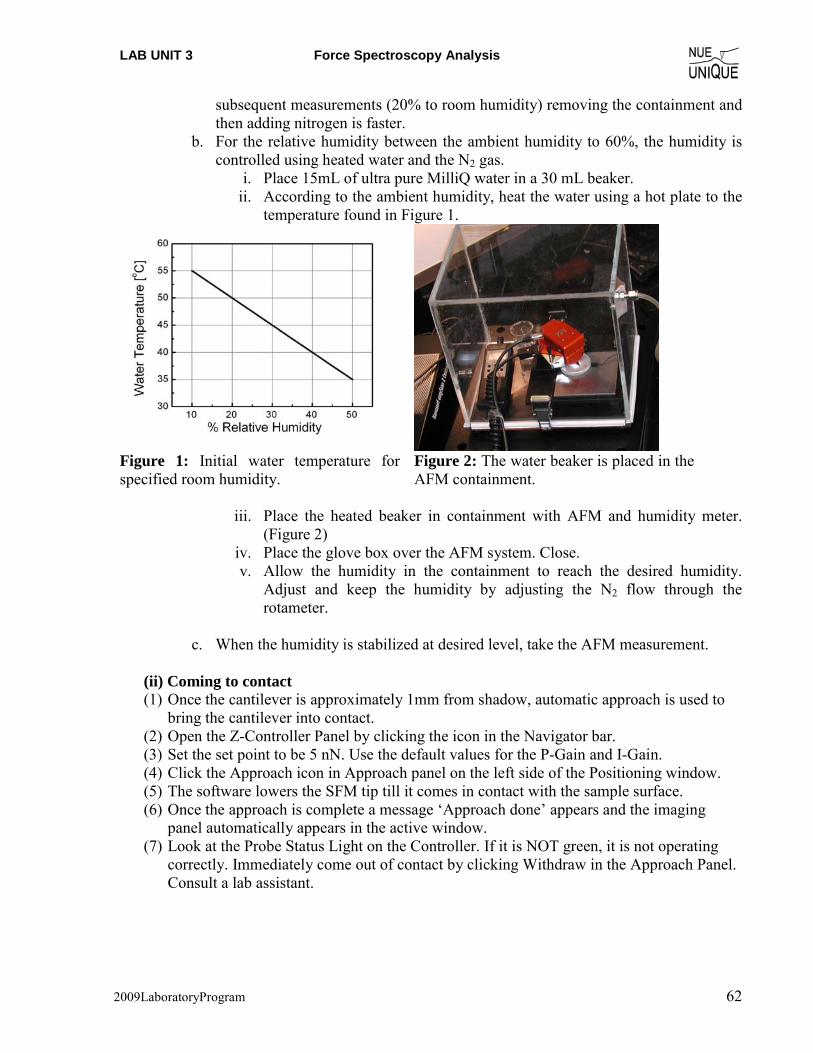
LAB UNIT 3 Force Spectroscopy Analysis
2009LaboratoryProgram 62
subsequent measurements (20% to room humidity) removing the containment and then adding nitrogen is faster.
b. For the relative humidity between the ambient humidity to 60%, the humidity is controlled using heated water and the N2 gas.
i. Place 15mL of ultra pure MilliQ water in a 30 mL beaker. ii. According to the ambient humidity, heat the water using a hot plate to the
temperature found in Figure 1.
Figure 1: Initial water temperature for specified room humidity.
Figure 2: The water beaker is placed in the AFM containment.
iii. Place the heated beaker in containment with AFM and humidity meter.
(Figure 2) iv. Place the glove box over the AFM system. Close. v. Allow the humidity in the containment to reach the desired humidity.
Adjust and keep the humidity by adjusting the N2 flow through the rotameter.
c. When the humidity is stabilized at desired level, take the AFM measurement.
(ii) Coming to contact (1) Once the cantilever is approximately 1mm from shadow, automatic approach is used to
bring the cantilever into contact. (2) Open the Z-Controller Panel by clicking the icon in the Navigator bar. (3) Set the set point to be 5 nN. Use the default values for the P-Gain and I-Gain. (4) Click the Approach icon in Approach panel on the left side of the Positioning window. (5) The software lowers the SFM tip till it comes in contact with the sample surface. (6) Once the approach is complete a message ‘Approach done’ appears and the imaging
panel automatically appears in the active window. (7) Look at the Probe Status Light on the Controller. If it is NOT green, it is not operating
correctly. Immediately come out of contact by clicking Withdraw in the Approach Panel. Consult a lab assistant.
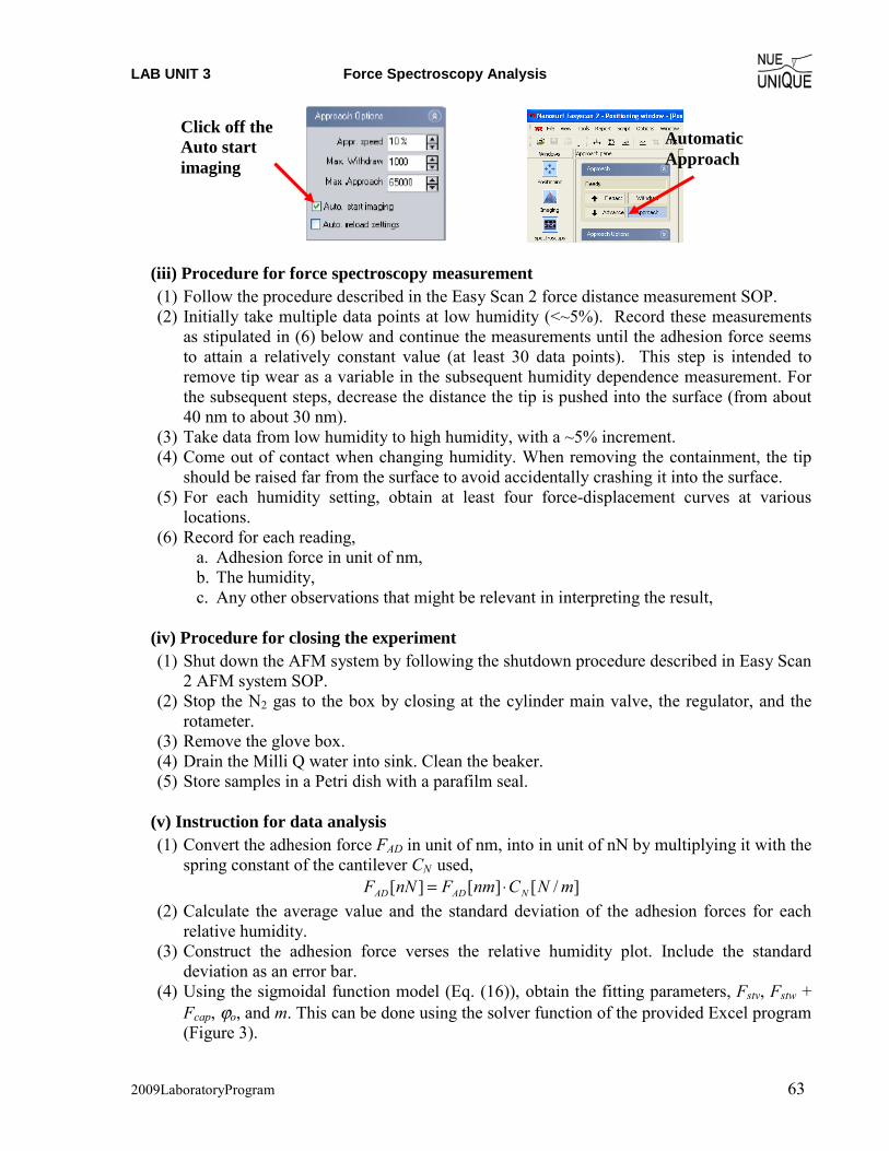
LAB UNIT 3 Force Spectroscopy Analysis
2009LaboratoryProgram 63
(iii) Procedure for force spectroscopy measurement
(1) Follow the procedure described in the Easy Scan 2 force distance measurement SOP. (2) Initially take multiple data points at low humidity (<~5%). Record these measurements
as stipulated in (6) below and continue the measurements until the adhesion force seems to attain a relatively constant value (at least 30 data points). This step is intended to remove tip wear as a variable in the subsequent humidity dependence measurement. For the subsequent steps, decrease the distance the tip is pushed into the surface (from about 40 nm to about 30 nm).
(3) Take data from low humidity to high humidity, with a ~5% increment. (4) Come out of contact when changing humidity. When removing the containment, the tip
should be raised far from the surface to avoid accidentally crashing it into the surface. (5) For each humidity setting, obtain at least four force-displacement curves at various
locations. (6) Record for each reading,
a. Adhesion force in unit of nm, b. The humidity, c. Any other observations that might be relevant in interpreting the result,
(iv) Procedure for closing the experiment
(1) Shut down the AFM system by following the shutdown procedure described in Easy Scan 2 AFM system SOP.
(2) Stop the N2 gas to the box by closing at the cylinder main valve, the regulator, and the rotameter.
(3) Remove the glove box. (4) Drain the Milli Q water into sink. Clean the beaker. (5) Store samples in a Petri dish with a parafilm seal.
(v) Instruction for data analysis
(1) Convert the adhesion force FAD in unit of nm, into in unit of nN by multiplying it with the spring constant of the cantilever CN used,
]/[][][ mNCnmFnNF NADAD ⋅= (2) Calculate the average value and the standard deviation of the adhesion forces for each
relative humidity. (3) Construct the adhesion force verses the relative humidity plot. Include the standard
deviation as an error bar. (4) Using the sigmoidal function model (Eq. (16)), obtain the fitting parameters, Fstv, Fstw +
Fcap, ϕo, and m. This can be done using the solver function of the provided Excel program (Figure 3).
Automatic Approach
Click off the Auto start imaging
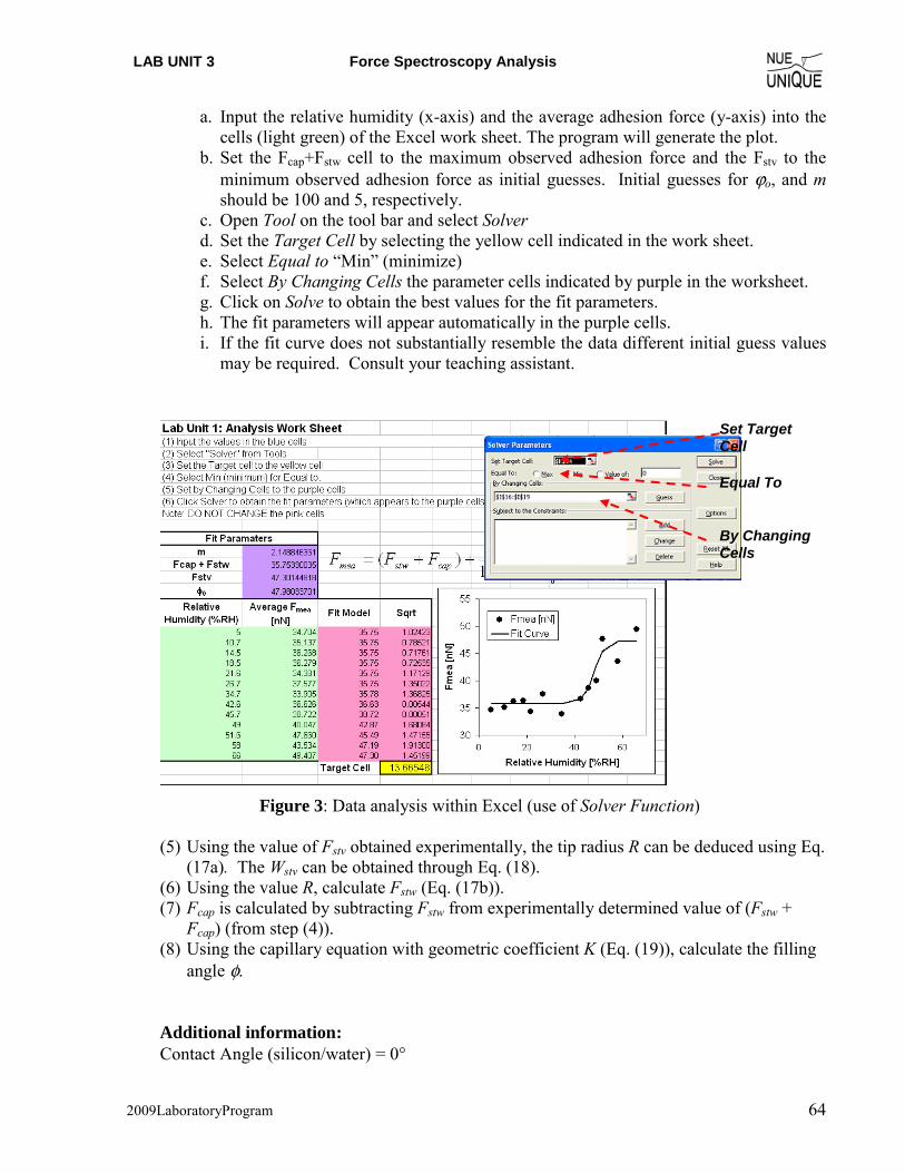
LAB UNIT 3 Force Spectroscopy Analysis
2009LaboratoryProgram 64
a. Input the relative humidity (x-axis) and the average adhesion force (y-axis) into the cells (light green) of the Excel work sheet. The program will generate the plot.
b. Set the Fcap+Fstw cell to the maximum observed adhesion force and the Fstv to the minimum observed adhesion force as initial guesses. Initial guesses for ϕo, and m should be 100 and 5, respectively.
c. Open Tool on the tool bar and select Solver d. Set the Target Cell by selecting the yellow cell indicated in the work sheet. e. Select Equal to “Min” (minimize) f. Select By Changing Cells the parameter cells indicated by purple in the worksheet. g. Click on Solve to obtain the best values for the fit parameters. h. The fit parameters will appear automatically in the purple cells. i. If the fit curve does not substantially resemble the data different initial guess values
may be required. Consult your teaching assistant.
Figure 3: Data analysis within Excel (use of Solver Function)
(5) Using the value of Fstv obtained experimentally, the tip radius R can be deduced using Eq. (17a). The Wstv can be obtained through Eq. (18).
(6) Using the value R, calculate Fstw (Eq. (17b)). (7) Fcap is calculated by subtracting Fstw from experimentally determined value of (Fstw +
Fcap) (from step (4)). (8) Using the capillary equation with geometric coefficient K (Eq. (19)), calculate the filling
angle φ.
Additional information: Contact Angle (silicon/water) = 0°
By Changing Cells
Equal To
Set Target Cell
LAB UNIT 3 Force Spectroscopy Analysis
2009LaboratoryProgram 65
γSiO/air = 100 mJ/m2 γSiO/waterr = 24.5 mJ/m2 γwater = 72.8 mJ/m2
(v) Silicon Treatment Prior to Experiment
The pretreatment of silicon addresses organic condamination. Safety (1) Follow the general rules for Nanotechnology Wet-Chemistry Lab at your Institution. (2) The UV/Ozone cleaner should be OFF before opening the sample tray. (3) Always handle silicon wafers with tweezers, not with your fingers. Wafer edges can be very sharp. (4) All solvent wastes are disposed into designated waste bottles located under the hood. (5) All silicon waste are disposed into the sharp object waste box. Depending on the degree of condamination solvent cleaning and UV/Ozone treatment are recommended.
Materials (1) 4 pieces of Silicon wafers ( ~1cm2 size pieces) (2) Millipore H2O (3) Acetone (4) Methanol (5) A 150 ml beaker, a caddy and a watch glass for sonication (6) A waste beaker for organic solvent (7) A plastic waste beaker. (8) Fine point tweezers (9) N2 gas with 0.2 micron filter. (10) 3 Petri dishes and para-film for finished samples. (11) UV/Ozone cleaner. (12) Sonicator (13) DI water
Procedure (1) Solvent cleaning: Removes organics off of the silicon surfaces.
a. Place silicon wafers in the caddy fitted in a 150 ml beaker and pour Acetone to fill upto~ 60 ml. b. Fill the sonicator with water. Place the beaker and adjust amount of water so that the water in the
sonicator is about at the surface level of Acetone in the beaker. c. Cover with the watch glass. d. Turn on the sonicator and run for 15 minutes. e. Turn off the sonicator and remove the beaker. f. Lift up the caddy (with silicon wafers) and drain the acetone into a waste beaker. Place the caddy
back into the beaker. g. Pour small amount of methanol for rinsing. Drain the methanol into the waste beaker. Repeat
once. h. Fill the beaker with Methanol upto ~ 60 ml. i. Place the beaker back in to the sonicator. Cover with the watch glass. j. Sonicate for 30 minutes. Take the beaker out when done. k. Lift the caddy and pour out the methanol into the waste beaker. Rinse with Millipore water at least
three times. Return the caddy back into the beaker and fill with Millipore water. l. Pick up a piece of wafers with tweezers and rinse with flowing Millipore water. Blowdry it with
N2 gas. m. Place the dried silicon wafers in a Petri dish. Cover the Petri dish.
LAB UNIT 3 Force Spectroscopy Analysis
2009LaboratoryProgram 66
n. Transfer the waste solvent mixture (of acetone, methanol and water) into the designated solvent waste bottle. Rinse the waste beaker with DI water. The spent water is also drained into the waste bottle. Note: Don’t use this waste beaker for the HF process.
o. Empty out the sonicator and allow drying.
(2) UV/Ozone treatment: Removes any trace of organics off of the surface.
a. Make sure the UV/Ozone cleaner is OFF. b. Open the sample tray and place two of the silicon wafers. Leave the other two for HF treatment. c. Close the tray. d. Turn on the power switch. e. Set a timer to 30 minutes and start. f. Turn of the power switch when done. Open the sample tray and take the silicon wafers out and
place them into a Petri dish and seal it with parafilm.
LAB UNIT 3 Force Spectroscopy Analysis
2009LaboratoryProgram 67
4. Background: Non-Covalent Short Range Interactions and Capillary Forces Table of Contents:
Motivation ................................................................................................................. 67 Short Range Interactions and Surface Forces............................................................ 67 Van der Waals Interactions for Point Interactions .................................................... 69 Surface Forces ........................................................................................................... 70 Hamaker Constant ..................................................................................................... 71 Van der Waals Retardation Effects ........................................................................... 72 Adhesion and Surface Energies................................................................................. 72 Cutoff Distance for Van der Waals Calculations ...................................................... 73 Capillary Forces due to Vapor Condensation ........................................................... 74 Critical Humidity for Capillary Neck Formation ...................................................... 75 Estimation of the Tip Radius Utilizing the Capillary Effects ................................... 76 Modification of Hydrophobicity (Wettability).......................................................... 78 Force Displacement Curves ...................................................................................... 79 References ................................................................................................................. 80 Recommended Reading............................................................................................. 80
Motivation As technology moves more towards miniaturization in novel product developments, it is
imperative to integrate interfacial interactions into design strategies. Consequently, interfacial forces have to be explored. Interfacial forces are on the order of 10-6 to 10-10 N, strong enough, for instance, to freeze gears in micro-electrical mechanical systems (MEMS), to affect the stability of colloidal system, or to wipe out magnetically stored data information in hard drives. There are multiple ways of exploring the strength of interfacial interactions, one of which is by force spectroscopy, also known as force-displacement (FD) analysis. The FD analysis involves a nanometer sharp scanning force microscopy (SFM) tip that is moved relative to the sample surface in nanometer to micrometer per second, as illustrated at end of this document in Figure 10. Before we discuss FD analysis, we first discuss interaction forces, particularly weak interactions between molecules and solids.
Short Range Interactions and Surface Forces There are three aspects that are of particular importance for any interaction: Its strength,
the distance over which it acts, and the environment through which it acts. Short range interactions, as summarized in Table 1, can be of following nature: ionic, covalent, metallic, or dipolar origin. Ionic, covalent, metallic and hydrogen bonds are so-called atomic forces that are important for forming strongly bonded condensed matter. These short range forces arise from the overlap of electron wave functions. Interactions of dipolar nature are classified further into strong hydrogen bonds and weak Van der Waals (VdW) interactions. They arise from dipole-
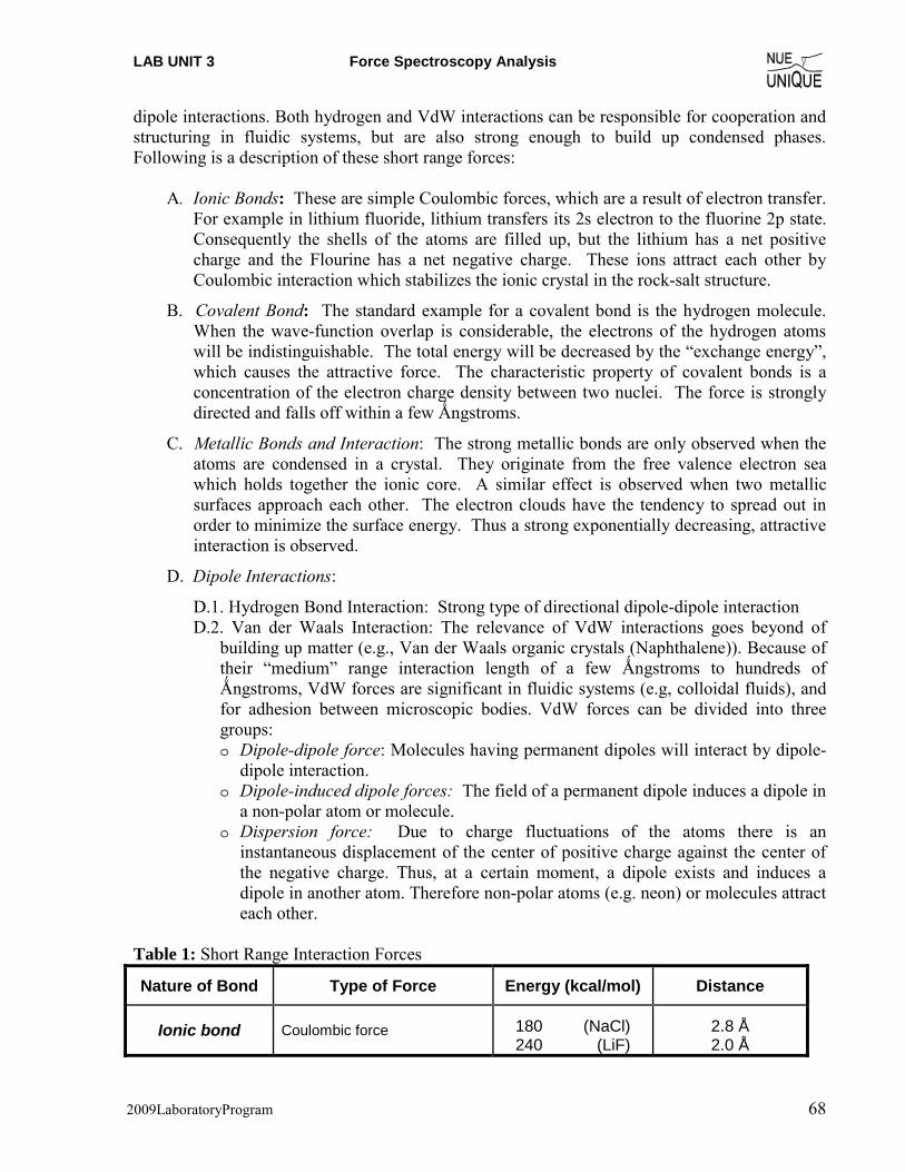
LAB UNIT 3 Force Spectroscopy Analysis
2009LaboratoryProgram 68
dipole interactions. Both hydrogen and VdW interactions can be responsible for cooperation and structuring in fluidic systems, but are also strong enough to build up condensed phases. Following is a description of these short range forces:
A. Ionic Bonds: These are simple Coulombic forces, which are a result of electron transfer.
For example in lithium fluoride, lithium transfers its 2s electron to the fluorine 2p state. Consequently the shells of the atoms are filled up, but the lithium has a net positive charge and the Flourine has a net negative charge. These ions attract each other by Coulombic interaction which stabilizes the ionic crystal in the rock-salt structure.
B. Covalent Bond: The standard example for a covalent bond is the hydrogen molecule. When the wave-function overlap is considerable, the electrons of the hydrogen atoms will be indistinguishable. The total energy will be decreased by the “exchange energy”, which causes the attractive force. The characteristic property of covalent bonds is a concentration of the electron charge density between two nuclei. The force is strongly directed and falls off within a few Ǻngstroms.
C. Metallic Bonds and Interaction: The strong metallic bonds are only observed when the atoms are condensed in a crystal. They originate from the free valence electron sea which holds together the ionic core. A similar effect is observed when two metallic surfaces approach each other. The electron clouds have the tendency to spread out in order to minimize the surface energy. Thus a strong exponentially decreasing, attractive interaction is observed.
D. Dipole Interactions:
D.1. Hydrogen Bond Interaction: Strong type of directional dipole-dipole interaction
D.2. Van der Waals Interaction: The relevance of VdW interactions goes beyond of building up matter (e.g., Van der Waals organic crystals (Naphthalene)). Because of their “medium” range interaction length of a few Ǻngstroms to hundreds of Ǻngstroms, VdW forces are significant in fluidic systems (e.g, colloidal fluids), and for adhesion between microscopic bodies. VdW forces can be divided into three groups: o Dipole-dipole force: Molecules having permanent dipoles will interact by dipole-
dipole interaction. o Dipole-induced dipole forces: The field of a permanent dipole induces a dipole in
a non-polar atom or molecule. o Dispersion force: Due to charge fluctuations of the atoms there is an
instantaneous displacement of the center of positive charge against the center of the negative charge. Thus, at a certain moment, a dipole exists and induces a dipole in another atom. Therefore non-polar atoms (e.g. neon) or molecules attract each other.
Table 1: Short Range Interaction Forces
Nature of Bond Type of Force Energy (kcal/mol) Distance
Ionic bond Coulombic force
180 (NaCl) 240 (LiF)
2.8 Å 2.0 Å

LAB UNIT 3 Force Spectroscopy Analysis
2009LaboratoryProgram 69
Covalent bond Electrostatic force (wave function overlap)
170 (Diamond) 283 (SiC)
N/A
Metallic bond free valency electron sea interaction (sometimes also partially covalent (e.g., Fe and W)
26 (Na) 96 (Fe) 210 (W)
4.3 Å 2.9 Å 3.1 Å
Hydrogen Bond a strong type of directional dipole-dipole interaction
7 (HF)
Van der Waals (i) dipole-dipole force (ii) dipole-induced dipole force (iii) dispersion forces (charge fluctuation)
2.4 (CH4)
significant in the range of a few Å to hundreds of Å
Van der Waals Interactions for Point Interactions The attractive VdW pair potential between point particles (i.e., atoms or small nonpolar
spherical molecule) is proportional to 1/r6, where r is the distance between the point particles. The widely used semi-empirical potential to describe VdW interactions is the Lennard-Jones (LJ) potential, referred to as the 6-12 potential because of its (1/r)6 and (1/r)12 distance r dependence of the attractive interaction and repulsive component, respectively. While the 6-potential is derived from point particle dipole-dipole interaction, the 12-potential is based on pure empiricism. The LJ potential is provided in the following two equivalent forms as function of the particle-particle distance r:
⎥⎥
⎦
⎤
⎢⎢
⎣
⎡⎟⎠
⎞⎜⎝
⎛ σ−⎟⎠
⎞⎜⎝
⎛ σε=+−=φ612
126 4rrr
C
rC)r( repvdw (1a)
where
rep
vdw
vdw
rep
CC;
CC
4
261
=ε⎟⎟⎠
⎞⎜⎜⎝
⎛=σ (1b)
Cvdw and Crep are characteristic constants. C = Cvdw is called the VdW interaction parameter. The empirical constant ε represents the characteristic energy of interaction between the molecules (the maximum energy of attraction between a pair of molecules). σ, a characteristic diameter of the molecule (also called the collision diameter), is the distance between two atoms (or molecules) for φ(r) = 0. The LJ potential is depicted in Figure 4..
Surface Forces The integral form of interaction forces between surfaces of macroscopic bodies through a third medium (e.g., vacuum and vapor) are called surfaces forces. To apply the VdW formalism to macroscopic bodies, one has to integrate the point interaction form presented above.
Figure 4: Lennard Jones (6-12) potential (empirical Van der Waals Potential between two atoms or nonpolar molecules).
r
φ(ε)
0
r(ε)
ε
σ
-
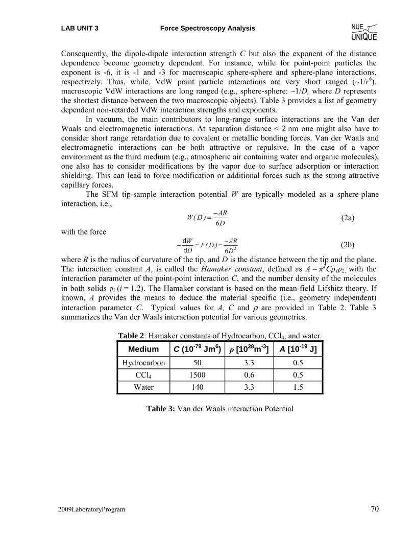
LAB UNIT 3 Force Spectroscopy Analysis
2009LaboratoryProgram 70
Consequently, the dipole-dipole interaction strength C but also the exponent of the distance dependence become geometry dependent. For instance, while for point-point particles the exponent is -6, it is -1 and -3 for macroscopic sphere-sphere and sphere-plane interactions, respectively. Thus, while, VdW point particle interactions are very short ranged (~1/r6), macroscopic VdW interactions are long ranged (e.g., sphere-sphere: ~1/D, where D represents the shortest distance between the two macroscopic objects). Table 3 provides a list of geometry dependent non-retarded VdW interaction strengths and exponents.
In vacuum, the main contributors to long-range surface interactions are the Van der Waals and electromagnetic interactions. At separation distance < 2 nm one might also have to consider short range retardation due to covalent or metallic bonding forces. Van der Waals and electromagnetic interactions can be both attractive or repulsive. In the case of a vapor environment as the third medium (e.g., atmospheric air containing water and organic molecules), one also has to consider modifications by the vapor due to surface adsorption or interaction shielding. This can lead to force modification or additional forces such as the strong attractive capillary forces.
The SFM tip-sample interaction potential W are typically modeled as a sphere-plane interaction, i.e.,
DAR)D(W
6−= (2a)
with the force 26D
AR)D(FDW −==−�
� (2b)
where R is the radius of curvature of the tip, and D is the distance between the tip and the plane. The interaction constant A, is called the Hamaker constant, defined as A = π2Cρ1ρ2, with the interaction parameter of the point-point interaction C, and the number density of the molecules in both solids ρi (i = 1,2). The Hamaker constant is based on the mean-field Lifshitz theory. If known, A provides the means to deduce the material specific (i.e., geometry independent) interaction parameter C. Typical values for A, C and ρ are provided in Table 2. Table 3 summarizes the Van der Waals interaction potential for various geometries.
Table 2: Hamaker constants of Hydrocarbon, CCl4, and water.
Medium C (10-79 Jm6) ρ [1028m-3] A [10-19 J] Hydrocarbon 50 3.3 0.5
CCl4 1500 0.6 0.5 Water 140 3.3 1.5
Table 3: Van der Waals interaction Potential
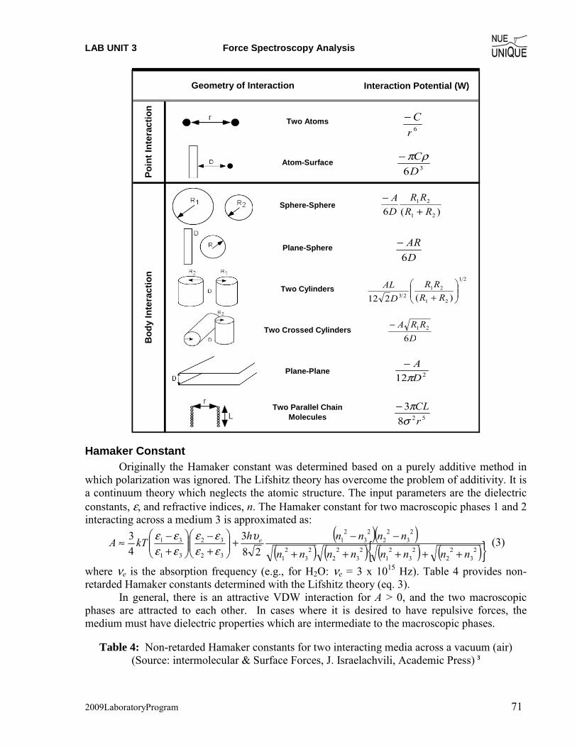
LAB UNIT 3 Force Spectroscopy Analysis
2009LaboratoryProgram 71
Interaction Potential (W)
Two Atoms
Atom-Surface
Sphere-Sphere
Plane-Sphere
Two Cylinders
Two Crossed Cylinders
Plane-Plane
Two Parallel Chain Molecules
Poin
t Int
erac
tion
Bod
y In
tera
ctio
n
Geometry of Interaction
6rC−
36DCρπ−
)(6 21
21
RRRR
DA
+−
DAR
6−
21
21
2123 )(212 ⎟⎟
⎠
⎞⎜⎜⎝
⎛
+ RRRR
DAL
DRRA
621−
212 DA
π−
5283
rCL
σπ−
Hamaker Constant Originally the Hamaker constant was determined based on a purely additive method in
which polarization was ignored. The Lifshitz theory has overcome the problem of additivity. It is a continuum theory which neglects the atomic structure. The input parameters are the dielectric constants, ε, and refractive indices, n. The Hamaker constant for two macroscopic phases 1 and 2 interacting across a medium 3 is approximated as:
( )( )( ) ( ) ( ) ( ){ }2
32
22
32
12
32
22
32
1
23
22
23
21
32
32
31
31
283
43
nnnnnnnn
nnnnhkTA e
+++++
−−+⎟⎟⎠
⎞⎜⎜⎝
⎛
+−
⎟⎟⎠
⎞⎜⎜⎝
⎛
+−≈ υ
εεεε
εεεε (3)
where νe is the absorption frequency (e.g., for H2O: νe = 3 x 10¹⁵ Hz). Table 4 provides non-retarded Hamaker constants determined with the Lifshitz theory (eq. 3). In general, there is an attractive VDW interaction for A > 0, and the two macroscopic phases are attracted to each other. In cases where it is desired to have repulsive forces, the medium must have dielectric properties which are intermediate to the macroscopic phases.
Table 4: Non-retarded Hamaker constants for two interacting media across a vacuum (air) (Source: intermolecular & Surface Forces, J. Israelachvili, Academic Press) 3
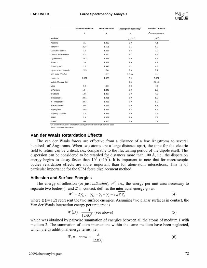
LAB UNIT 3 Force Spectroscopy Analysis
2009LaboratoryProgram 72
Dielectric constant Refractive Index Absorption frequencya Hamaker Constant
ε n ν Amedium/air/medium
Medium (1015s-1) (10-20)
Acetone 21 1.359 2.9 4.1
Benzene 2.28 1.501 2.1 5.0
Calcium Flouride 7.4 1.427 3.8 7.0
Carbon tetrachloride 2.24 1.460 2.7 5.5
Cyclohexane 2.03 1.426 2.9 5.2
Ethanol 26 1.361 3.0 4.2
Fused quartz 3.8 1.448 3.2 6.3
Hydrocarbon (crystal) 2.25 1.50 3.0 7.1
Iron oxide (Fe3O4) 1.97 3.0 est 21
Liquid He 1.057 1.028 5.9 0.057
Metals (Au. Ag, Cu) 3-5 25--40
Mica 7.0 1.60 3.0 10
n-Pentane 1.84 1.349 3.0 3.8
n-Octane 1.95 1.387 3.0 4.5
n-Dodecane 2.01 1.411 3.0 5.0
n-Tetradecane 2.03 1.418 2.9 5.0
n-Hexadecane 2.05 1.423 2.9 5.1
Polystyrene 2.55 1.557 2.3 6.5
Polyvinyl chloride 3.2 1.527 2.9 7.5
PTFE 2.1 1.359 2.9 3.8
Water 80 1.333 3.0 3.7aUV absorption frequencies obtained from Cauchy plots mainly from Hough and White (1980) and H. Christenson (1983, thesis).
Van der Waals Retardation Effects The van der Waals forces are effective from a distance of a few Ǻngstroms to several hundreds of Ǻngstroms. When two atoms are a large distance apart, the time for the electric field to return can be critical, i.e., comparable to the fluctuating period of the dipole itself. The dispersion can be considered to be retarded for distances more than 100 Å, i.e., the dispersion energy begins to decay faster than 1/r6 (~1/r7). It is important to note that for macroscopic bodies retardation effects are more important than for atom-atom interactions. This is of particular importance for the SFM force displacement method.
Adhesion and Surface Energies The energy of adhesion (or just adhesion), W", i.e., the energy per unit area necessary to
separate two bodies (1 and 2) in contact, defines the interfacial energy γ12 as: 21211212 22 γγγγγγ −+== ;W '' (4)
where γi (i= 1,2) represent the two surface energies. Assuming two planar surfaces in contact, the Van der Waals interaction energy per unit area is
( ) 21 12 DADW
π−= (see above) (5)
which was obtained by pairwise summation of energies between all the atoms of medium 1 with medium 2. The summation of atom interactions within the same medium have been neglected, which yields additional energy terms, i.e.,
22 12 oDA.constW
π+−= (6)
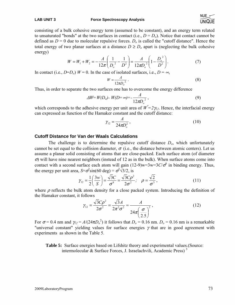
LAB UNIT 3 Force Spectroscopy Analysis
2009LaboratoryProgram 73
consisting of a bulk cohesive energy term (assumed to be constant), and an energy term related to unsaturated "bonds" at the two surfaces in contact (i.e., D = Do). Notice that contact cannot be defined as D = 0 due to molecular repulsive forces. Do is called the "cutoff distance". Hence the total energy of two planar surfaces at a distance D ≥ Do apart is (neglecting the bulk cohesive energy)
⎟⎟⎠
⎞⎜⎜⎝
⎛−=⎟⎟
⎠
⎞⎜⎜⎝
⎛−−=+= 2
2
22221 112
1112 D
DDA
DDAWWW o
oo ππ. (7)
In contact (i.e., D=Do) W = 0. In the case of isolated surfaces, i.e., D = ∞, 212 oD
AWπ
= . (8)
Thus, in order to separate the two surfaces one has to overcome the energy difference
ΔW=W(Do)- W(D=∞)=- 212 oDA
π, (9)
which corresponds to the adhesive energy per unit area of W''=2γ12. Hence, the interfacial energy can expressed as function of the Hamaker constant and the cutoff distance:
212 24 oDAπ
γ = , (10)
Cutoff Distance for Van der Waals Calculations The challenge is to determine the repulsive cutoff distance Do, which unfortunately
cannot be set equal to the collision diameter, σ (i.e., the distance between atomic centers). Let us assume a planar solid consisting of atoms that are close-packed. Each surface atom (of diameter σ) will have nine nearest neighbors (instead of 12 as in the bulk). When surface atoms come into contact with a second surface each atom will gain (12-9)w=3w=3C/σ6 in binding energy. Thus, the energy per unit area, S=σ2sin(60 deg) = σ2√3/2, is
32
2
8122
2333
21
σρ
σρ
σγ ===⎟
⎠
⎞⎜⎝
⎛= ;CCSw , (11)
where ρ reflects the bulk atom density for a close packed system. Introducing the definition of the Hamaker constant, it follows
2222
2
12
5224
23
23
⎟⎠
⎞⎜⎝
⎛≈==
.
AACσπ
σπσργ , (12)
For σ = 0.4 nm and γ12 = A/(24πDo2) it follows that Do = 0.16 nm. Do = 0.16 nm is a remarkable
"universal constant" yielding values for surface energies γ that are in good agreement with experiments as shown in the Table 5.
Table 5: Surface energies based on Lifshitz theory and experimental values.(Source: intermolecular & Surface Forces, J. Israelachvili, Academic Press) 3
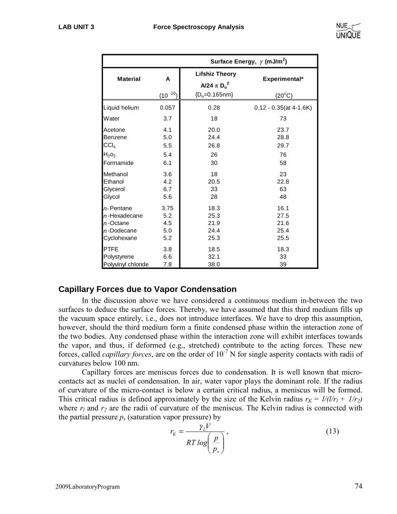
LAB UNIT 3 Force Spectroscopy Analysis
2009LaboratoryProgram 74
Lifshiz Theory
A/24 π Do2
(10 -20) {Do=0.165nm} (20oC)
Liquid helium 0.057 0.28 0.12 - 0.35(at 4-1.6K)
Water 3.7 18 73
Acetone 4.1 20.0 23.7Benzene 5.0 24.4 28.8CCl4 5.5 26.8 29.7H2o2 5.4 26 76Formamide 6.1 30 58
Methanol 3.6 18 23Ethanol 4.2 20.5 22.8Glycerol 6.7 33 63Glycol 5.6 28 48
n- Pentane 3.75 18.3 16.1n -Hexadecane 5.2 25.3 27.5n -Octane 4.5 21.9 21.6n -Dodecane 5.0 24.4 25.4Cyclohexane 5.2 25.3 25.5
PTFE 3.8 18.5 18.3Polystyrene 6.6 32.1 33Polyvinyl chloride 7.8 38.0 39
Material A
Surface Energy, γ (mJ/m2)
Experimental*
Capillary Forces due to Vapor Condensation In the discussion above we have considered a continuous medium in-between the two
surfaces to deduce the surface forces. Thereby, we have assumed that this third medium fills up the vacuum space entirely, i.e., does not introduce interfaces. We have to drop this assumption, however, should the third medium form a finite condensed phase within the interaction zone of the two bodies. Any condensed phase within the interaction zone will exhibit interfaces towards the vapor, and thus, if deformed (e.g., stretched) contribute to the acting forces. These new forces, called capillary forces, are on the order of 10-7 N for single asperity contacts with radii of curvatures below 100 nm.
Capillary forces are meniscus forces due to condensation. It is well known that micro-contacts act as nuclei of condensation. In air, water vapor plays the dominant role. If the radius of curvature of the micro-contact is below a certain critical radius, a meniscus will be formed. This critical radius is defined approximately by the size of the Kelvin radius rK = l/(l/rl + 1/r2) where rl and r2 are the radii of curvature of the meniscus. The Kelvin radius is connected with the partial pressure ps (saturation vapor pressure) by
⎟⎟⎠
⎞⎜⎜⎝
⎛=
s
LK
pplogRT
Vr γ , (13)
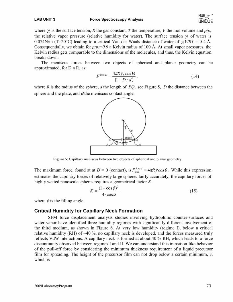
LAB UNIT 3 Force Spectroscopy Analysis
2009LaboratoryProgram 75
where γL is the surface tension, R the gas constant, T the temperature, V the mol volume and p/ps
the relative vapor pressure (relative humidity for water). The surface tension γL of water is 0.074N/m (T=20°C) leading to a critical Van der Waals distance of water of γLV/RT = 5.4 Å. Consequentially, we obtain for p/ps=0.9 a Kelvin radius of 100 Å. At small vapor pressures, the Kelvin radius gets comparable to the dimensions of the molecules, and thus, the Kelvin equation breaks down. The meniscus forces between two objects of spherical and planar geometry can be approximated, for D « R, as:
( )d/DcosRF LDR
+Θ=>>
14 γπ , (14)
where R is the radius of the sphere, d the length of PQ , see Figure 5, D the distance between the sphere and the plate, and θ the meniscus contact angle.
Figure 5: Capillary meniscus between two objects of spherical and planar geometry
The maximum force, found at at D = 0 (contact), is θγπ cosRF dR
max 4=>> . While this expression estimates the capillary forces of relatively large spheres fairly accurately, the capillary forces of highly wetted nanoscale spheres requires a geometrical factor K.
φφ
cos4)cos1( 2
⋅+=K (15)
where φ is the filling angle.
Critical Humidity for Capillary Neck Formation SFM force displacement analysis studies involving hydrophilic counter-surfaces and
water vapor have identified three humidity regimes with significantly different involvement of the third medium, as shown in Figure 6. At very low humidity (regime I), below a critical relative humidity (RH) of ~40 %, no capillary neck is developed, and the forces measured truly reflects VdW interactions. A capillary neck is formed at about 40 % RH, which leads to a force discontinuity observed between regimes I and II. We can understand this transition-like behavior of the pull-off force by considering the minimum thickness requirement of a liquid precursor film for spreading. The height of the precursor film can not drop below a certain minimum, e, which is
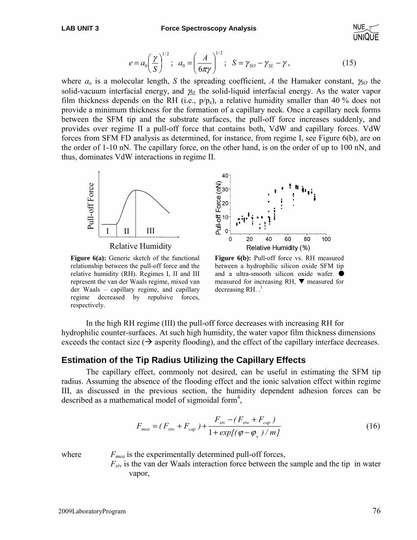
LAB UNIT 3 Force Spectroscopy Analysis
2009LaboratoryProgram 76
2/1
0 ⎟⎠
⎞⎜⎝
⎛=S
ae γ ; 2/1
0 6 ⎟⎟⎠
⎞⎜⎜⎝
⎛=πγAa ; γγγ −−= SLSOS , (15)
where ao is a molecular length, S the spreading coefficient, A the Hamaker constant, γSO the solid-vacuum interfacial energy, and γSL the solid-liquid interfacial energy. As the water vapor film thickness depends on the RH (i.e., p/ps), a relative humidity smaller than 40 % does not provide a minimum thickness for the formation of a capillary neck. Once a capillary neck forms between the SFM tip and the substrate surfaces, the pull-off force increases suddenly, and provides over regime II a pull-off force that contains both, VdW and capillary forces. VdW forces from SFM FD analysis as determined, for instance, from regime I, see Figure 6(b), are on the order of 1-10 nN. The capillary force, on the other hand, is on the order of up to 100 nN, and thus, dominates VdW interactions in regime II.
Pull-
off F
orce
Relative Humidity
I II III
Figure 6(a): Generic sketch of the functional relationship between the pull-off force and the relative humidity (RH). Regimes I, II and III represent the van der Waals regime, mixed van der Waals – capillary regime, and capillary regime decreased by repulsive forces, respectively.
Figure 6(b): Pull-off force vs. RH measured between a hydrophilic silicon oxide SFM tip and a ultra-smooth silicon oxide wafer. ● measured for increasing RH, ▼ measured for decreasing RH. .1
In the high RH regime (III) the pull-off force decreases with increasing RH for
hydrophilic counter-surfaces. At such high humidity, the water vapor film thickness dimensions exceeds the contact size (� asperity flooding), and the effect of the capillary interface decreases.
Estimation of the Tip Radius Utilizing the Capillary Effects The capillary effect, commonly not desired, can be useful in estimating the SFM tip
radius. Assuming the absence of the flooding effect and the ionic salvation effect within regime III, as discussed in the previous section, the humidity dependent adhesion forces can be described as a mathematical model of sigmoidal form4,
]m/)exp[()FF(F
)FF(F capstwstvcapstwmea
01 ϕϕ −+
+−++= (16)
where Fmea is the experimentally determined pull-off forces,
Fstv is the van der Waals interaction force between the sample and the tip in water vapor,
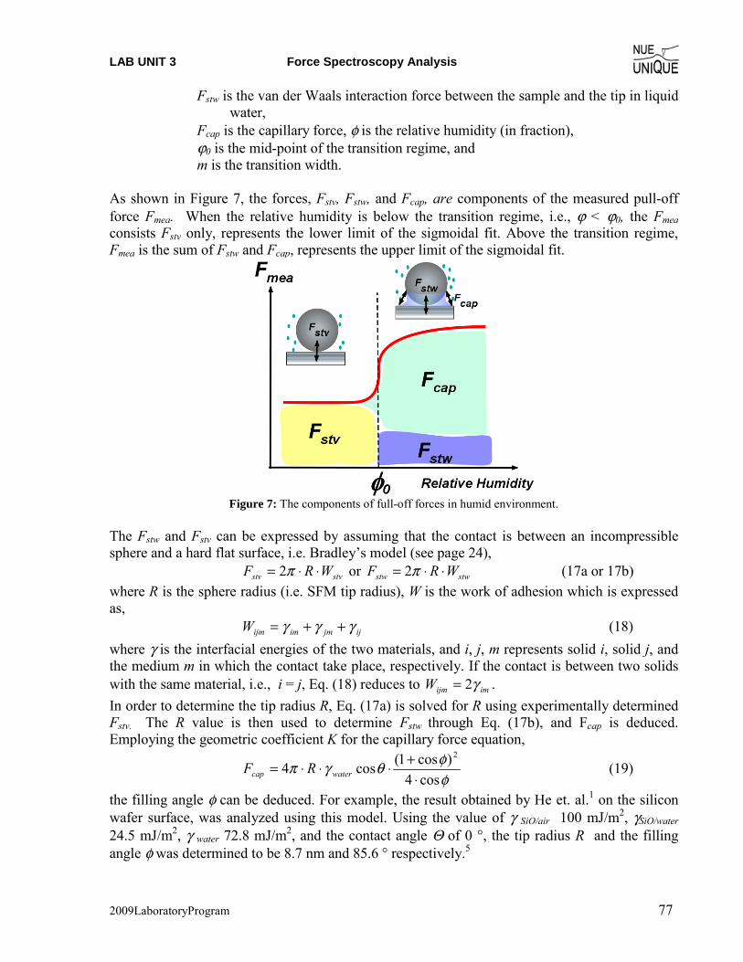
LAB UNIT 3 Force Spectroscopy Analysis
2009LaboratoryProgram 77
Fstw is the van der Waals interaction force between the sample and the tip in liquid water,
Fcap is the capillary force, φ is the relative humidity (in fraction), ϕ0 is the mid-point of the transition regime, and m is the transition width.
As shown in Figure 7, the forces, Fstv, Fstw, and Fcap, are components of the measured pull-off force Fmea. When the relative humidity is below the transition regime, i.e., ϕ < ϕ0, the Fmea consists Fstv only, represents the lower limit of the sigmoidal fit. Above the transition regime, Fmea is the sum of Fstw and Fcap, represents the upper limit of the sigmoidal fit.
Figure 7: The components of full-off forces in humid environment.
The Fstw and Fstv can be expressed by assuming that the contact is between an incompressible sphere and a hard flat surface, i.e. Bradley’s model (see page 24),
stvstv WRF ⋅⋅= π2 or stwstw WRF ⋅⋅= π2 (17a or 17b) where R is the sphere radius (i.e. SFM tip radius), W is the work of adhesion which is expressed as,
ijjmimijmW γγγ ++= (18) where γ is the interfacial energies of the two materials, and i, j, m represents solid i, solid j, and the medium m in which the contact take place, respectively. If the contact is between two solids with the same material, i.e., i = j, Eq. (18) reduces to imijmW γ2= . In order to determine the tip radius R, Eq. (17a) is solved for R using experimentally determined Fstv. The R value is then used to determine Fstw through Eq. (17b), and Fcap is deduced. Employing the geometric coefficient K for the capillary force equation,
φφθγπ
cos4)cos1(cos4
2
⋅+⋅⋅⋅= watercap RF (19)
the filling angle φ can be deduced. For example, the result obtained by He et. al.1 on the silicon wafer surface, was analyzed using this model. Using the value of γ SiO/air 100 mJ/m2, γSiO/water 24.5 mJ/m2, γ water 72.8 mJ/m2, and the contact angle Θ of 0 °, the tip radius R and the filling angle φ was determined to be 8.7 nm and 85.6 ° respectively.5
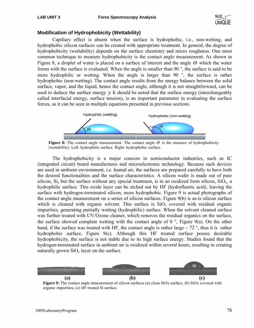
LAB UNIT 3 Force Spectroscopy Analysis
2009LaboratoryProgram 78
Modification of Hydrophobicity (Wettability) Capillary effect is absent when the surface is hydrophobic, i.e., non-wetting, and hydrophobic silicon surfaces can be created with appropriate treatment. In general, the degree of hydrophobicity (wettability) depends on the surface chemistry and micro roughness. One most common technique to measure hydrophobicity is the contact angle measurement. As shown in Figure 8, a droplet of water is placed on a surface of interest and the angle Θ which the water forms with the surface is evaluated. When the angle is smaller than 90 °, the surface is said to be more hydrophilic or wetting. When the angle is larger than 90 °, the surface is rather hydrophobic (non-wetting). The contact angle results from the energy balance between the solid surface, vapor, and the liquid, hence the contact angle, although it is not straightforward, can be used to deduce the surface energy γ. It should be noted that the surface energy (interchangeably called interfacial energy, surface tension), is an important parameter in evaluating the surface forces, as it can be seen in multiple equations presented in previous sections.
Figure 8: The contact angle measurement. The contact angle Θ is the measure of hydrophobicity (wettability). Left: hydrophilic surface. Right: hydrophobic surface.
The hydrophobicity is a major concern in semiconductor industries, such as IC (integrated circuit) board manufactures and microelectronic technology. Because such devices are used in ambient environment, i.e. humid air, the surfaces are prepared carefully to have both the desired functionalities and the surface characteristics. A silicon wafer is made out of pure silicon, Si, but the surface without any special treatment, is in an oxidized form silicon, SiOx, a hydrophilic surface. This oxide layer can be etched out by HF (hydrofluoric acid), leaving the surface with hydrogen-terminated silicon, more hydrophobic. Figure 9 is actual photographs of the contact angle measurement on a series of silicon surfaces. Figure 9(b) is as-is silicon surface which is cleaned with organic solvent. This surface is SiOx covered with residual organic impurities, generating partially wetting (hydrophilic) surface. When the solvent cleaned surface was further treated with UV/Ozone cleaner, which removes the residual organics on the surface, the surface showed complete wetting with the contact angle of 0 °, Figure 9(a). On the other hand, if the surface was treated with HF, the contact angle is rather large ~ 72 °, thus it is rather hydrophobic surface, Figure 9(c). Although this HF treated surface posses desirable hydrophobicity, the surface is not stable due to its high surface energy. Studies found that the hydrogen-terminated surface in ambient air is oxidized within several hours, resulting in creating naturally grown SiOx layer on the surface.
(a) (b) (c)
Figure 9: The contact angle measurement of silicon surfaces (a) clean SiOx surface, (b) SiOx covered with organic impurities, (c) HF treated Si surface.
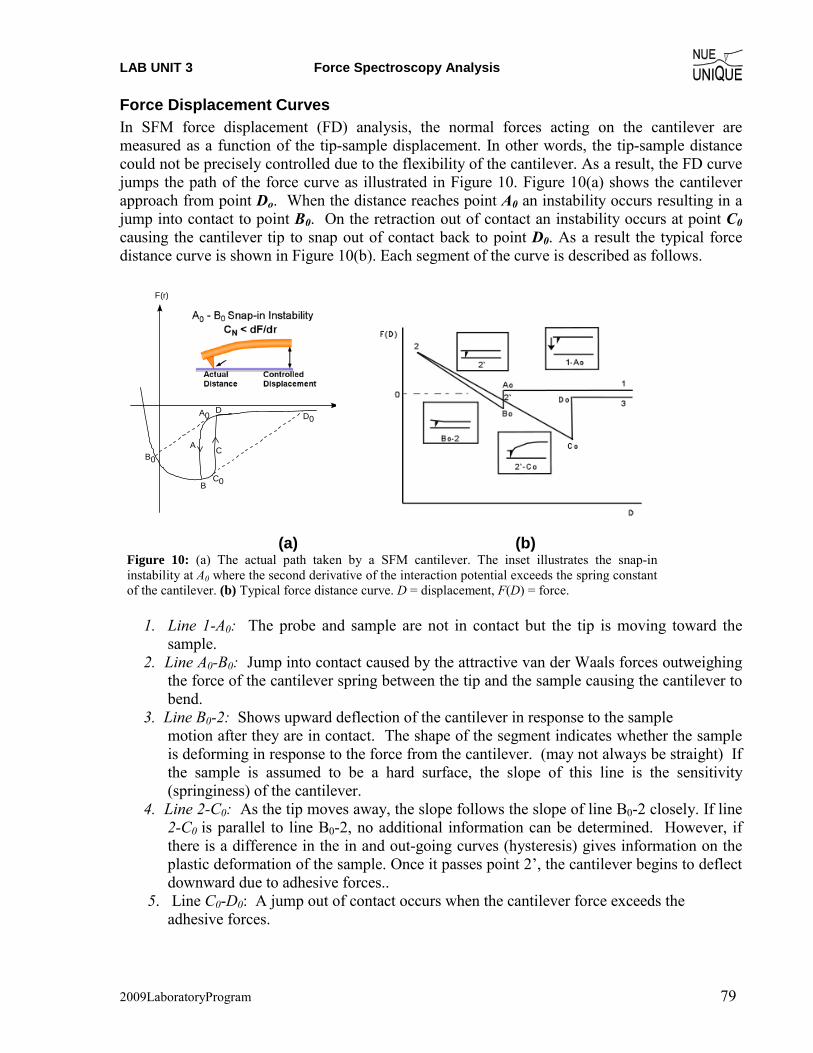
LAB UNIT 3 Force Spectroscopy Analysis
2009LaboratoryProgram 79
Force Displacement Curves In SFM force displacement (FD) analysis, the normal forces acting on the cantilever are measured as a function of the tip-sample displacement. In other words, the tip-sample distance could not be precisely controlled due to the flexibility of the cantilever. As a result, the FD curve jumps the path of the force curve as illustrated in Figure 10. Figure 10(a) shows the cantilever approach from point Do. When the distance reaches point A0 an instability occurs resulting in a jump into contact to point B0. On the retraction out of contact an instability occurs at point C0 causing the cantilever tip to snap out of contact back to point D0. As a result the typical force distance curve is shown in Figure 10(b). Each segment of the curve is described as follows.
F(r)
CA
B
D
C0
D0
B0
A0
(a) (b) Figure 10: (a) The actual path taken by a SFM cantilever. The inset illustrates the snap-in instability at A0 where the second derivative of the interaction potential exceeds the spring constant of the cantilever. (b) Typical force distance curve. D = displacement, F(D) = force.
1. Line 1-A0: The probe and sample are not in contact but the tip is moving toward the
sample. 2. Line A0-B0: Jump into contact caused by the attractive van der Waals forces outweighing
the force of the cantilever spring between the tip and the sample causing the cantilever to bend.
3. Line B0-2: Shows upward deflection of the cantilever in response to the sample motion after they are in contact. The shape of the segment indicates whether the sample
is deforming in response to the force from the cantilever. (may not always be straight) If the sample is assumed to be a hard surface, the slope of this line is the sensitivity (springiness) of the cantilever.
4. Line 2-C0: As the tip moves away, the slope follows the slope of line B0-2 closely. If line 2-C0 is parallel to line B0-2, no additional information can be determined. However, if there is a difference in the in and out-going curves (hysteresis) gives information on the plastic deformation of the sample. Once it passes point 2’, the cantilever begins to deflect downward due to adhesive forces..
5. Line C0-D0: A jump out of contact occurs when the cantilever force exceeds the adhesive forces.
LAB UNIT 3 Force Spectroscopy Analysis
2009LaboratoryProgram 80
The jump out of contact distance will always be greater than the jump into contact distance because of few possible causes are:
a. During contact, some adhesive bonds are created. b. During contact, the sample buckles and “wraps” around the tip, increasing the
contact area. c. Hysteresis contributions d. Capillary forces exerted by contaminants such as water.
FD analysis is widely used for adhesion and force interaction studies. Recently biological
materials have been studied by force spectroscopy, such as adsorption strength of proteins on a substrate and folding/unfolding energy of DNAs.
References 1 M. He, A. Blum, D. E. Aston, C. Buenviaje, and R. M. Overney, Journal of chemical physics
114 (3), 1355 (2001). 2 H. Hertz, J. Reine und Angewandte Mathematik 92, 156 (1882). 3 J. N. Israelachvili, Intermolecular and surface forces. (Academic Press, London, 1992). 4 D. L. Sedin and K. L. Rowlen, Analytical Chemistry 72, 2183 (2000). 5 C. Ziebert and K. H. Zum Gahr, Tribology Letters 17 (4), 901 (2004). 6 J. A. Greenwood, Proc. R. Soc. Lond. A 453, 1277 (1997).
Recommended Reading
Contact Mechanics by K. L. Johnson, Cambridge University Press, Cambridge, 1985. Gases, liquids and solids and other states of matter by D. Tabor, Cambridge Univ. Press,
Cambridge, 3rd ed. 2000. Intermolecular and surface forces by J. N. Israelachvili, Academic Press, London, 1992. Nanoscience: Friction and Rheology on the Nanometer Scale by E. Meyer, R. M. Overney, K.
Dransfeld, and T. Gyalog, World Scientific Publ., Singapore, 1998.
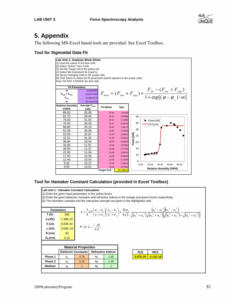
LAB UNIT 3 Force Spectroscopy Analysis
2009LaboratoryProgram 81
5. Appendix The following MS-Excel based tools are provided. See Excel Toolbox.
Tool for Sigmoidal Data Fit
Lab Unit 1: Analysis Work Sheet
(2) Select "Solver" from Tools (3) Set the Target cell to the yellow cell(4) Select Min (minimum) for Equal to.(5) Set by Changing Cells to the purple cells(6) Click Solver to obtain the fit parameters (which appears to the purple cells)Note: DO NOT CHANGE the pink cells
m 0.80950955Fcap + Fstw 32.86757066
Fstv 10.58973278
ϕ0 40.39442756
Relative Humidity (%RH)
Average Fmea
[nN]Fit Model Sqrt
88.00 25.05 32.87 7.81293
81.70 29.40 32.87 3.46988
76.00 31.63 32.87 1.23269
70.40 33.33 32.87 0.46706
68.60 34.15 32.87 1.28173
62.39 35.05 32.87 2.18528
53.94 32.87 32.87 0.00002
42.51 31.34 31.34 0.00001
39.84 18.04 18.04 0.00001
33.00 11.57 10.59 0.97950
28.50 11.37 10.59 0.77533
22.90 11.04 10.59 0.45478
17.00 10.59 10.59 0.00000
12.40 10.43 10.59 0.16249
9.30 10.21 10.59 0.38416
8.50 10.01 10.59 0.57933Target Cell 19.78519
Fit Paramaters
(1) Input the values in the blue cells.
5
10
15
20
25
30
35
40
0.00 20.00 40.00 60.00 80.00
Relative Humidity [%RH]
Fmea
[nN
]
Fmea [nN]Fit Curve
]/)exp[(1)(
)(0
mFFF
FFF capstwstvcapstwmea ϕϕ −+
+−++=
Tool for Hamaker Constant Calculation (provided in Excel Toolbox)
Lab Unit 1: Hamaker Constant Calculation(1) Enter the given input parameters in the yellow boxes(2) Enter the given dielectric constants and refractive indices in the orange and green boxes respectively(3) The Hamaker constant and the interaction strength are given in the highlighted cells
T (K) 300k (J/K) 1.38E-23h (Js) 6.63E-34υε
(Hz) 3.00E+15R (nm) 50D0 (nm) 0.16
A[J] W[J]Phase 1 ε1 3.78 n1 1.45 5.97E-20 -3.11E-18Phase 2 ε2 3.78 n2 1.45Medium ε3 1 n3 1
Parameters
Dielectric Constants Refractive IndicesMaterial Properites
( )( )( ) ( ) ( ) ( ){ }2
32
22
32
12
32
22
32
1
23
22
23
21
32
32
31
31
283
43
nnnnnnnn
nnnnhkTA e
+++++
−−+⎟⎟⎠
⎞⎜⎜⎝
⎛
+−
⎟⎟⎠
⎞⎜⎜⎝
⎛
+−≈ υ
εεεε
εεεε
( )DARDW
6−=

LAB UNIT 3 Force Spectroscopy Analysis
2009LaboratoryProgram 82
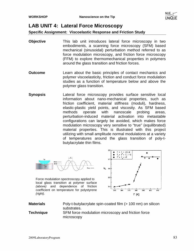
WORKSHOP Nanoscience on the Tip
2009LaboratoryProgram 83
LAB UNIT 4: Lateral Force Microscopy Specific Assignment: Viscoelastic Response and Friction Study Objective This lab unit introduces lateral force microscopy in two
embodiments, a scanning force microscopy (SFM) based mechanical (sinusoidal) perturbation method referred to as force modulation microscopy, and friction force microscopy (FFM) to explore thermomechanical properties in polymers around the glass transition and friction forces.
Outcome Learn about the basic principles of contact mechanics and
polymer viscoelasticity, friction and conduct force modulation studies as a function of temperature below and above the polymer glass transition.
Synopsis Lateral force microscopy provides surface sensitive local
information about nano-mechanical properties, such as friction coefficient, material stiffness (moduli), hardness, elastic-plastic yield points, and viscosity. As SFM based methods operate with nanoscale probing areas, perturbation-induced material activation into metastable configurations can largely be avoided, which makes force modulation microscopy very sensitive to “true” (equilibrated) material properties. This is illustrated with this project utilizing with small amplitude normal modulations at a variety of temperatures around the glass transition of poly-t-butylacrylate thin films.
Force modulation spectroscopy applied to local glass transition at polymer surface (above) and dependence of friction coefficient on temperature for polystyrene (right).
Materials Poly-t-butylacrylate spin-coated film (> 100 nm) on silicon
substrates. Technique SFM force modulation microscopy and friction force
microscopy
LAB UNIT 4 Force Modulation Microscopy
2009LaboratoryProgram 84
Table of Contents
1. Assignment ............................................................................................. 85 2. Quiz – Preparation for the Experiment.................................................. 86
Theoretical Questions....................................................................................................................... 86 Prelab Quiz....................................................................................................................................... 86
3. Experimental Assignment...................................................................... 89
Goal .................................................................................................................................................. 89 Safety................................................................................................................................................ 89 Instrumental Setup............................................................................................................................ 89 Materials........................................................................................................................................... 89 Experimental Procedure ................................................................................................................... 89
4. Background: Friction, Contact Mechanics and Viscoelastic
Phenomena of Polymers........................................................................ 97 Stress-Strain Relationships............................................................................................................... 97 Classical Understanding of Friction ................................................................................................. 99 The Bowden-Tabor Adhesion Model of Friction ........................................................................... 100 Models of Single Asperity Contact ................................................................................................ 101 Contact Mechanics – Fully Elastic Models .................................................................................... 102 Force Modulation SFM and Hertzian Theory ................................................................................ 104 Contact Stiffness ............................................................................................................................ 106 Force Modulation and Polymer Relaxation Properties................................................................... 106 Transition and Viscoelasticity ........................................................................................................ 107 Introduction to Linear Viscoelasticity ............................................................................................ 109 Time-Temperature Equivalence of Viscoelastic Behaviors ........................................................... 112 Glass Transition.............................................................................................................................. 113 References ...................................................................................................................................... 115 Recommended Reading.................................................................................................................. 116
LAB UNIT 4 Lateral Force Microscopy
2009LaboratoryProgram 85
1. Assignment The assignment is to locally investigate the nano-thermomechanical properties of thin film polymers utilizing friction force microscopy and shear modulation force microscopy, and to employ the theories and background information to discuss the experimental results. The steps are:
1. Familiarize yourself with the background information provided in Section 4. 2. Test your background knowledge with the provided Quiz in Section 2. 3. Conduct the friction and force modulation experiments in Section 3. Follow the
experimental step-by-step procedure. 4. Analyze your data as described in Section 3 5. Finally, provide a report with the following information:
(i) Results section: In this section you show your data and discuss instrumental details (i.e., limitations) and the quality of your data (error analysis).
(ii) Discussion section: In this section you discuss and analyze your data in the light of the provided background information.
It is also appropriate to discuss section (i) and (ii) together. (iii) Summary and outlook: Here you summarize your findings and provide an
outlook on how one could use the technique in other fields. The report is evaluated based on the quality of the discussion and the integration of your experimental data and the provided theory. You are encouraged to discuss results that are unexpected. It is important to include discussions on the causes for discrepancies and inconsistencies in the data.
LAB UNIT 4 Force Modulation Microscopy
2009LaboratoryProgram 86
2. Quiz – Preparation for the Experiment Theoretical Questions (1) (3pts) Determine the contact area for a JKR contact at which the contact becomes
unstable. (2) (3pts) Describe the two terms solid-like and liquid-like using the two simple models
of Hooke’s law of elasticity and Newton’s law of viscosity. (3) (3pts) List methods that are use to determine the glass transition temperature. What
property are they actually sensitive to? (4) (3pts) At the glass transition temperature, the response signal of SM-FM that is
proportional to the contact stiffness is increasing noticeably. Considering that the modulus for many polymers decreases by orders of magnitude from the glassy state to the rubbery state (e.g., in the case of polystyrene PS by about 4 orders of magnitude from 109 N/m2 to 105 N/m2), the probing contact area of SM-FM has to increase substantially to compensate for the reduction in the material stiffness. This is based on the Herzian relationship between the contact stiffness and the modulus, i.e, kc = 2aE (for normal distortion), or kc=8aG (for lateral distortion). Evaluate with the Hertzian model, the relative degree of contact area increase for polystyrene.
(5) (3pts) Glass transition and Gibbs free energy. (a) Show in a V(T) diagram the distinct difference between melt/freezing transition
and a glass transition (b) How are changes related to the specific heat and volume obtained from Gibbs
free energy.
Prelab Quiz (1) (10 pts) For a sinusoidal FM microscopy experiments, the input modulation
amplitude Ain and the output signal amplitude Aout shall be known in volts that are applied to the piezo (PZ) and received from the photo diode (PD), respectively. The conversion sensitivity factors SPZ and SPD are used to convert the two signals into nanometer.
(a) Determine formally the root mean square (RMS) amplitudes in nanometer. (b) With the appropriate RMS amplitudes determine the force that is acting on a
cantilever with spring constant kL. (c) Assuming an ideal spring model as depicted in Figure 3, what is the force acting
on the sample? (d) Provide an expression for the sample deformation δ as function of Ain and Aout. (e) Express the the contact stiffness as function of δ, Ain, Aout and kL.
LAB UNIT 4 Lateral Force Microscopy
2009LaboratoryProgram 87
(2) (a) (5 pts) Explain why Amontons’ law is generally valid, i.e., why friction force is generally not a function of contact area. Under what types of circumstances could it be a function of contact area?
(b) (5 pts) Applied normal force, FN, can be distinguished from total normal force, FTOT, by the inclusion of adhesion force, FADH, in the latter term. Often, FN and FTOT must be calculated based on force distance curve data and other information. This can be accomplished according to:
( )ADHBTSPN
TOT FFFS
CF +−= − or ( )BTSPN
N FFS
CF −−=
where FSP is the set point signal, FT-B is the out of contact normal photodiode signal, CN is the cantilever spring constant and S is the normal sample stiffness. Calculate FN and FTOT from the following sets of data:
Set A Set B FSP 10 nA 35 nN CN (nominal) 0.2 N/m 0.2 N/m CN (actual) 0.115 N/m 0.134 N/m S 0.04 nA/nm 0.88 nm/nm FT-B -3 nA 10 nm FADH 12.6 nA 230 nm
Which should be used when determining friction coefficient? Why?
(3) (10 pts) FM microscopy utilized a function generator with a sinusoidal input modulation to the piezo. The cantilever response modulation signal Aoutsin(ωt+φout) is detected with a laser detection scheme by the photodiode. Because the signals are very small, i.e., within the noise level of the signal, a lock-in technique is used. The lock-in amplifier compares the photodiode signal with the input signal to the piezo, Ainsin(ωt+φin), as a reference signal. Note that both signals are not only defined by their amplitude and frequency but also by their phase φ. The output signal of the lock-in amplifier Vpsd is the product of two sine waves, i.e.,
VPSD = AinAout sin(ωt+φin) sin(ωt+φout) This signal is composed of two AC signals, one with frequency ωin+ωout and ωin-ωout and is heavily low pass filtered. Consequently, as in our case, only a non-zero DC signal comes through for ωin = ωout = ω. In other words the lock-in technique is frequency discriminating the signal it receives based on the reference signal. The quantities that matter are the amplitudes, and the phase shift φ = φin- φin. As the phase of the phase signal of the input signal to the piezo is arbitrary, we will define it generally as zero, i.e., φin = 0. The situation described here, is illustrated in the figure below, expressing the frequency discriminated signal VPSD in complex form, i.e.,
( )φ+ω= t*PSD ReV

LAB UNIT 4 Force Modulation Microscopy
2009LaboratoryProgram 88
Describe the operation of the function generator. How would you expect the phase angle to differ between solid-like and liquid-like materials?
4) Below, data are provided from a friction-load experiment of Octadecyl-Phosphonic Acid (ODPA). Based on these data:
a) Determine the shear strength properties (i.e., α and τoA) of the materials at 29 oC and 94 oC, according to the model of Bowden/Tabor.
b) Provide reasons for the differences in values.
Input Modulation Signal (Piezo): A1(ω) =Ainsin(ωt)
Response Modulation Signal (Photodiode), A2(ω) =Aoutsin(ωt+φ)
Amplitude
Time Time Delay Δt=Tφ/2π
T
x
iy
R φ
R cos(φ)
R sin(φ)
R = SLock-In Aout
P
O
OHOH
ODPA
P
O
OHOH P
O
OHOH P
O
OHOH
ODPA
LAB UNIT 4 Lateral Force Microscopy
2009LaboratoryProgram 89
3. Experimental Assignment Goal Following the step-by-step instructions below, determine the glass transition temperature of the PTBA film and measure the friction coefficient as a function of temperature. Analyze and discuss the data with the background information provided in Section 4. Provide a written report of this experiment. Specifically provide answers to the following questions:
(1) What is the observed glass transition temperature for poly (t-butyl acrylate)? Does this value correlate with the literature value? What factors would cause the observed Tg value to be different from the literature?
(2) Why is Modulated Force Microscopy effective at determining the glass transition temperature?
(3) How does the friction coefficient change as a function of temperature? Does this compare well to the results of Sills et al. for polystyrene (p. 83, lower right)?
(4) Can you determine the glass transition from the friction data? How does it compare to that obtained from the previous method?
Safety - Wear safety glasses. - Refer to the General rules in the AFM lab. - The heating module should be off when it is not in use.
Instrumental Setup - Nanosurf Easy Scan 2 Flex AFM system with long contact Mode SFM tip with
0.2 N/m spring constant with NO Aluminum coating. - Two heating stages with controllers - Lock-in amplifier and function generator with two long BNC cables - Oscilloscope
Materials - Samples: 2 pieces of pre-prepared (by TA) ~ 1cm2 Spin-coated PtBA film on
silicon substrate, stored in sealed Petri dishes until ready for the experiment. The sample PtBA (Mw = 137.3k) is spin cast onto an organic contaminant-cleaned (possibly also oxide treated) silicon wafer and annealed above its glass transition temperature in a vacuum oven. Preferred film thicknesses are between 100 to 500 nm.
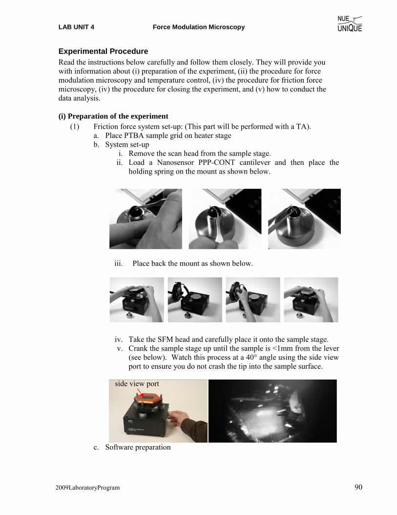
LAB UNIT 4 Force Modulation Microscopy
2009LaboratoryProgram 90
Experimental Procedure Read the instructions below carefully and follow them closely. They will provide you with information about (i) preparation of the experiment, (ii) the procedure for force modulation microscopy and temperature control, (iv) the procedure for friction force microscopy, (iv) the procedure for closing the experiment, and (v) how to conduct the data analysis. (i) Preparation of the experiment
(1) Friction force system set-up: (This part will be performed with a TA). a. Place PTBA sample grid on heater stage b. System set-up
i. Remove the scan head from the sample stage. ii. Load a Nanosensor PPP-CONT cantilever and then place the
holding spring on the mount as shown below.
iii. Place back the mount as shown below.
iv. Take the SFM head and carefully place it onto the sample stage. v. Crank the sample stage up until the sample is <1mm from the lever
(see below). Watch this process at a 40° angle using the side view port to ensure you do not crash the tip into the sample surface.
c. Software preparation
side view port
LAB UNIT 4 Lateral Force Microscopy
2009LaboratoryProgram 91
i. Once the cantilever is loaded click on ‘Operating Mode’ icon in the menu list on the left side of the screen in the Easyscan 2 software. The operating mode panel will appear. Select ‘CONTR’ as the mounted cantilever and ‘Static Force’ as the operating mode.
ii. Click on the ‘Imaging’ icon (top right). Select the ‘Topography – Scan Forward’ plot. Add two new plots by clicking the new chart icon twice (middle right). Next, select one of the new charts and change the signal of the first to ‘Deflection - Scan Forward’ by clicking the select signal icon (bottom right) and choosing amplitude from the drop down menu. Select the second new chart and change the signal to ‘Friction – Scan Forward’. Repeat this process for ‘Scan Backward’ plots for all three. Repeat this process again and make dual line graphs, rather than color maps for all three signals.
(2) Shear Modulation Force Microscopy system set-up: (This part will have been performed by the TA): a. Place the PTBA sample on the MMR heating stage.
i. Repeat the same procedure as above for setting up software and cantilever installation.
b. Connect BNC cables: i. from Function Generator Function output to X-Modulation BNC
ii. from Function Generator Function output to Lock-In REF IN signal (reference)
iii. from X Output BNC to Lock-In Signal A
LAB UNIT 4 Force Modulation Microscopy
2009LaboratoryProgram 92
(ii) Dry Dynamic Mode Imaging
1) Coming into contact: a. Once the cantilever is approximately 1mm from the surface, click on
the ‘Positioning’ icon and click ‘Approach’ to bring the lever into contact.
b. Close the frequency tuning window that appears. c. Ensure that the probe status light is green when approaching. If not, stop
the approach and consult your TA for the cause of this. Note that a blinking red light means that no lever is detected, while a solid red light means that a tip is detected but the frequency is not set properly.
d. The program will automatically switch to the imaging window once imaging begins.
2) Adjusting slope: a. Once imaging has begun, the slope will most likely need adjustment. b. This can be done automatically by selecting ‘Imaging – adjust slope’ from
the ‘Script’ menu. c. The software automatically adjusts slope and begins the scan again.
3) Optimize scan quality: a. Open the Z-Controller Panel (right) by clicking the z-
controller icon. b. Set the set point to be 50%. Use the default values for
the P-Gain and I-Gain. c. In the Imaging Panel, change the image width to 2μm and ensure that the
resolution is set to 256. d. Vary the set point, P-Gain, I-Gain and time/line values to optimize the
image quality according to the following guidelines: i. Faster scan speeds (lower time/line values) generally require higher
gains. ii. Excessively high gains cause the controller to ring, resulting in very
noisy amplitude and topography signals. iii. Very large surface features generally require higher gains or higher
amplitude or slower scan speed. iv. Noisy measurements may improve with increased set point, but very
high set points may result in coming out of contact. You may also employ the minimum force trick, that is, increase the set point (%) until you are out of contact and then decrease it again until a reasonable image is obtained. This results in using the minimum force.
4) Obtain images: a. Once scan quality is acceptable complete the scan by clicking on the
‘Finish’ icon. b. If the completed image looks good, click ‘Photo’ and save the image. c. Each image should be in a different area of the sample. To move to a
different area, simply select random values (from -20 to 20 μm) and input these into the ‘Image X-Pos’ and ‘Image Y-Pos’ fields in the imaging

LAB UNIT 4 Lateral Force Microscopy
2009LaboratoryProgram 93
panel. Alternatively, you may withdraw the cantilever under the ‘Positioning’ window and use the translation stage to move to a new area of the sample surface. Be sure to ‘Approach’ again after moving.
d. Click ‘Start’ to begin a new image. Repeat slope adjustment and image optimization as necessary.
e. Obtain at least three images for each sample. 5) Change sample:
a. Once all images have been obtained for that sample, go to the ‘Positioning’ window and click ‘Withdraw’.
b. Once the cantilever is well off the surface, click ‘Retract’ and raise the tip farther (~3 mm off the surface).
c. Remove the scan head from the surface and change the sample, making sure it is appropriately grounded.
d. Repeat steps 1)-5) for all samples. 6) Conclude imaging:
a. Come out of contact using ‘Withdraw’ and ‘Retract’. b. Remove the cantilever and store it appropriately. c. Shut down the Easyscan 2 software and turn off the controller.
LAB UNIT 4 Force Modulation Microscopy
2009LaboratoryProgram 94
(iii) Determining PtBA Glass Transition
(1) Ensure that the MMR stage initial temperature is set to 300K by inputting ‘SK300’ into the control box. Check the temperature by typing ‘TE’ and pressing enter.
(2) In the software, record the deflection signal value for out of contact. This can be performed by scanning while out of contact and watching the deflection dual line graph.
(3) Set PID gains to nominal values. (4) Coming into contact:
a. Once the cantilever is approximately 1mm from the surface, click on the ‘Positioning’ icon and click ‘Approach’ to bring the lever into contact.
b. Ensure that the probe status light is green when approaching. If not, stop the approach and consult your TA for the cause of this. Note that a blinking red light means that no lever is detected, while a solid red light means that a tip is detected but the frequency is not set properly.
c. The program will automatically switch to the imaging window once imaging begins. Click ‘Stop’ on the imaging panel to stop imaging.
(5) Scan the sample surface and identify a smooth area about 5μm in size. (6) Ensure that the function generator settings are as follows: frequency:
4300Hz, amplitude 0.5Vpp, offset 0Vpp. (7) Ensure that the lock-in amplifier settings are as follows:
i. Time Constant: 30ms, 6db. ii. SYNC: On.
iii. Sensitivity: ~ 200mV, but change if the amplitude meter bar is too large or too small.
iv. Signal input: A, AC, Floated Ground. v. Set Display: R (amplitude response), Θ (phase response).
vi. Check initial phase shift, and set to zero (right side display) (8) Wait 1-2 minutes for thermal equilibrium. (9) By hand, record for ~30 seconds the R and Θ values from the lock-in. (10) By changing the MMR set point, repeat steps 11-15 for temperatures from
300K to 335K in increments of 2.5K (11) Cool the system back to 300K (12) Withdraw tip, set heater temperature to 300K, set function generator
amplitude to 0. (13) Shut down the AFM system as instructed by your TA.
(iv) Determining PtBA Friction Coefficient (1) Ensure preparations described above have been performed. (2) Approach sample and come into contact per the above instructions. (3) Open heater software at Desktop:contactlab:HEATER-CONTROL:
TC-36-25RS232rev.A.exe (4) Initialize Heater in Heater program
a. Set FIXED SET TEMP to 25.00
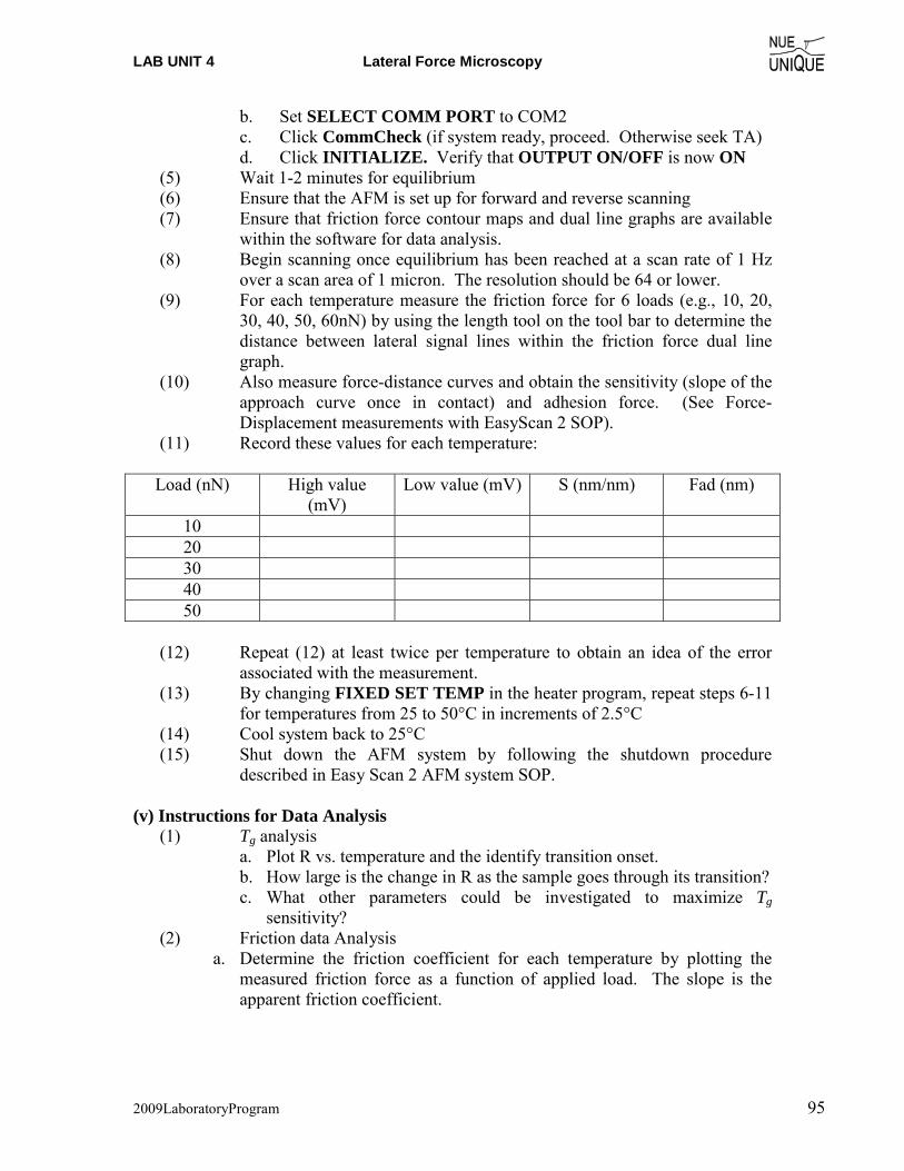
LAB UNIT 4 Lateral Force Microscopy
2009LaboratoryProgram 95
b. Set SELECT COMM PORT to COM2 c. Click CommCheck (if system ready, proceed. Otherwise seek TA) d. Click INITIALIZE. Verify that OUTPUT ON/OFF is now ON
(5) Wait 1-2 minutes for equilibrium (6) Ensure that the AFM is set up for forward and reverse scanning (7) Ensure that friction force contour maps and dual line graphs are available
within the software for data analysis. (8) Begin scanning once equilibrium has been reached at a scan rate of 1 Hz
over a scan area of 1 micron. The resolution should be 64 or lower. (9) For each temperature measure the friction force for 6 loads (e.g., 10, 20,
30, 40, 50, 60nN) by using the length tool on the tool bar to determine the distance between lateral signal lines within the friction force dual line graph.
(10) Also measure force-distance curves and obtain the sensitivity (slope of the approach curve once in contact) and adhesion force. (See Force-Displacement measurements with EasyScan 2 SOP).
(11) Record these values for each temperature:
Load (nN) High value (mV)
Low value (mV) S (nm/nm) Fad (nm)
10 20 30 40 50
(12) Repeat (12) at least twice per temperature to obtain an idea of the error
associated with the measurement. (13) By changing FIXED SET TEMP in the heater program, repeat steps 6-11
for temperatures from 25 to 50°C in increments of 2.5°C (14) Cool system back to 25°C (15) Shut down the AFM system by following the shutdown procedure
described in Easy Scan 2 AFM system SOP. (v) Instructions for Data Analysis
(1) Tg analysis a. Plot R vs. temperature and the identify transition onset. b. How large is the change in R as the sample goes through its transition? c. What other parameters could be investigated to maximize Tg
sensitivity? (2) Friction data Analysis
a. Determine the friction coefficient for each temperature by plotting the measured friction force as a function of applied load. The slope is the apparent friction coefficient.

LAB UNIT 4 Force Modulation Microscopy
2009LaboratoryProgram 96
b. Plot the resulting friction coefficients as a function of temperature. Compare this trend to that of polystyrene for Sills et al. How are they different, how are they similar?
c. Discuss why friction coefficient is a function of temperature. Could you predict the glass transition from the friction coefficient?
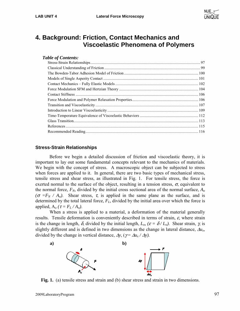
LAB UNIT 4 Lateral Force Microscopy
2009LaboratoryProgram 97
4. Background: Friction, Contact Mechanics and Viscoelastic Phenomena of Polymers
Table of Contents:
Stress-Strain Relationships............................................................................................................... 97 Classical Understanding of Friction ................................................................................................. 99 The Bowden-Tabor Adhesion Model of Friction ........................................................................... 100 Models of Single Asperity Contact ................................................................................................ 101 Contact Mechanics – Fully Elastic Models .................................................................................... 102 Force Modulation SFM and Hertzian Theory ................................................................................ 104 Contact Stiffness ............................................................................................................................ 106 Force Modulation and Polymer Relaxation Properties................................................................... 106 Transition and Viscoelasticity ........................................................................................................ 107 Introduction to Linear Viscoelasticity ............................................................................................ 109 Time-Temperature Equivalence of Viscoelastic Behaviors ........................................................... 112 Glass Transition.............................................................................................................................. 113 References ...................................................................................................................................... 115 Recommended Reading.................................................................................................................. 116
Stress-Strain Relationships
Before we begin a detailed discussion of friction and viscoelastic theory, it is important to lay out some fundamental concepts relevant to the mechanics of materials. We begin with the concept of stress. A macroscopic object can be subjected to stress when forces are applied to it. In general, there are two basic types of mechanical stress, tensile stress and shear stress, as illustrated in Fig. 1. For tensile stress, the force is exerted normal to the surface of the object, resulting in a tension stress, σ, equivalent to the normal force, FN, divided by the initial cross sectional area of the normal surface, Ao (σ =FN / Ao). Shear stress, τ, is applied in the same plane as the surface, and is determined by the total lateral force, FL, divided by the initial area over which the force is applied, Ao (τ = FL / Ao).
When a stress is applied to a material, a deformation of the material generally results. Tensile deformation is conveniently described in terms of strain, ε, where strain is the change in length, δ, divided by the initial length, Lo, (ε = δ / Lo). Shear strain, γ, is slightly different and is defined in two dimensions as the change in lateral distance, Δux, divided by the change in vertical distance, Δy, (γ = Δux / Δy).
a)
b)
Fig. 1. (a) tensile stress and strain and (b) shear stress and strain in two dimensions.

LAB UNIT 4 Force Modulation Microscopy
2009LaboratoryProgram 98
Figure 2 (a) provides a general diagram of stress as a function of strain in tension.
As shown, deformations can behave in a number of ways over a range of stress. First, if the strain resulting from a given stress disappears when the stress is removed, then the material is said to behave elastically and stress is a linear function of strain, as shown in the early portion of the curve in Fig. 2(a). In the case of elastic behavior, energy is stored within the system and a simple equation exists relating stress to strain, called Hooke’s Law after the English mathematician Robert Hooke (1635-1703):
εσ E= (1) where E is the modulus of elasticity (or Young’s modulus), which is a material property. Similarly, for shear stress:
γτ G= (2) where G is the shear modulus of the material. Beyond the yield point, or the elastic limit of the material, the strain will not return to zero after removal of the stress, as shown in Fig. 2(b), rather, a plastic deformation has taken place that has permanently deformed the material. a)
b)
Fig. 2. (a) General stress-strain relationship, (b) deformation beyond yield point, B, resulting in a plastic deformation where strain does not return to zero when the stress is removed.
To round out our discussion of stress-strain relationships, we should note that
when a solid material is stressed in tension, for example, strains other than the normal strain may be observed. So, when a strain is observed in the axial plane as a result of a normal stress (as in Fig. 1(a)), strain in the lateral directions are also observed as the radius of the rod “shrinks” to compensate for the elongation in length. French mathematician Simeon Denis Poisson (1781-1840) recognized this, and therefore we name the ratio of lateral strain to axial strain after him, Poisson’s ratio, ν:
strainaxialstrainlateral
__=ν (3)
When operating in the elastic regime, it can be shown that the shear modulus and the modulus of elasticity are related to Poisson’s ratio as:
( )ν+= 12GE (4)
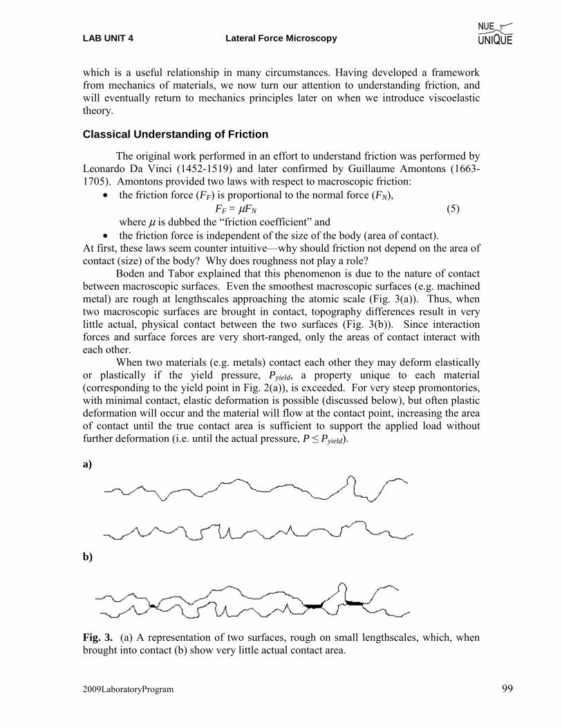
LAB UNIT 4 Lateral Force Microscopy
2009LaboratoryProgram 99
which is a useful relationship in many circumstances. Having developed a framework from mechanics of materials, we now turn our attention to understanding friction, and will eventually return to mechanics principles later on when we introduce viscoelastic theory.
Classical Understanding of Friction
The original work performed in an effort to understand friction was performed by Leonardo Da Vinci (1452-1519) and later confirmed by Guillaume Amontons (1663-1705). Amontons provided two laws with respect to macroscopic friction:
• the friction force (FF) is proportional to the normal force (FN), FF = μFN (5)
where μ is dubbed the “friction coefficient” and • the friction force is independent of the size of the body (area of contact).
At first, these laws seem counter intuitive—why should friction not depend on the area of contact (size) of the body? Why does roughness not play a role? Boden and Tabor explained that this phenomenon is due to the nature of contact between macroscopic surfaces. Even the smoothest macroscopic surfaces (e.g. machined metal) are rough at lengthscales approaching the atomic scale (Fig. 3(a)). Thus, when two macroscopic surfaces are brought in contact, topography differences result in very little actual, physical contact between the two surfaces (Fig. 3(b)). Since interaction forces and surface forces are very short-ranged, only the areas of contact interact with each other.
When two materials (e.g. metals) contact each other they may deform elastically or plastically if the yield pressure, Pyield, a property unique to each material (corresponding to the yield point in Fig. 2(a)), is exceeded. For very steep promontories, with minimal contact, elastic deformation is possible (discussed below), but often plastic deformation will occur and the material will flow at the contact point, increasing the area of contact until the true contact area is sufficient to support the applied load without further deformation (i.e. until the actual pressure, P ≤ Pyield). a)
b)
Fig. 3. (a) A representation of two surfaces, rough on small lengthscales, which, when brought into contact (b) show very little actual contact area.
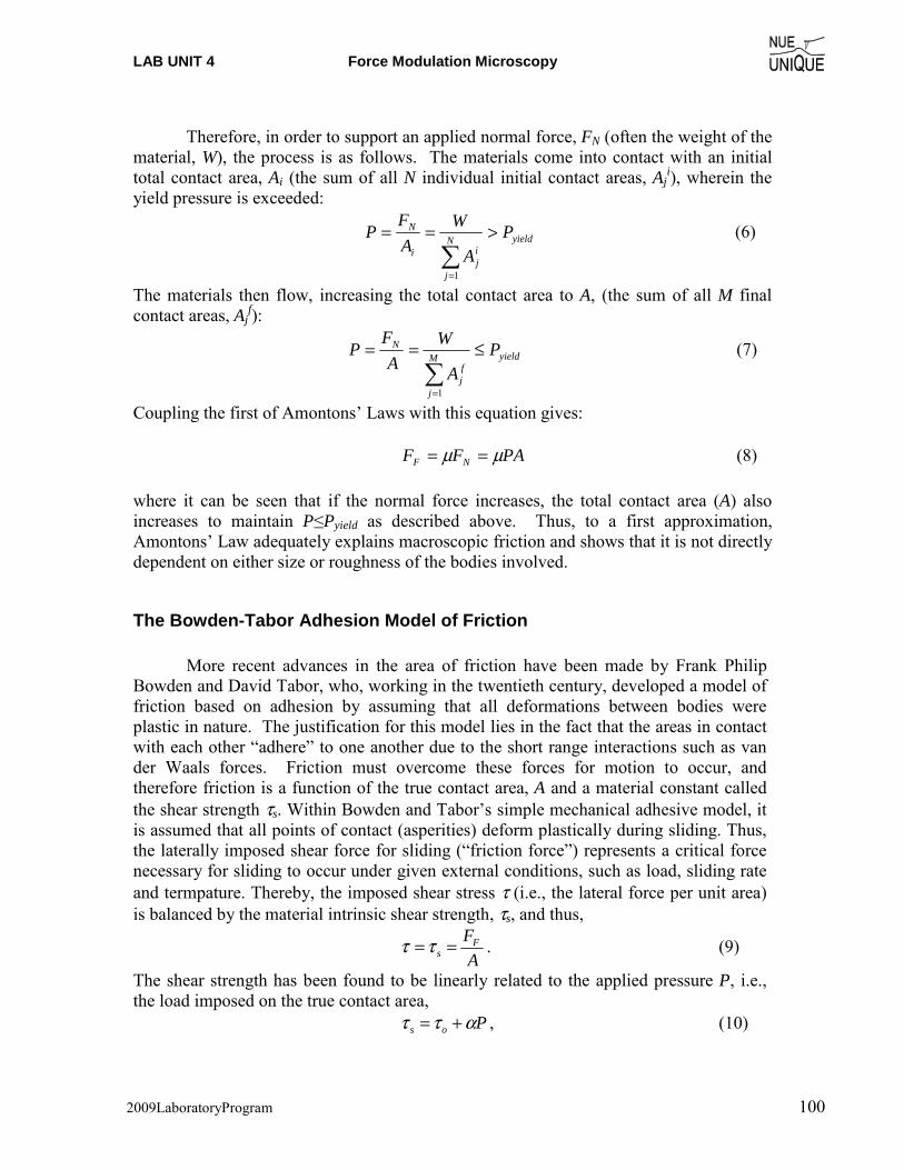
LAB UNIT 4 Force Modulation Microscopy
2009LaboratoryProgram 100
Therefore, in order to support an applied normal force, FN (often the weight of the
material, W), the process is as follows. The materials come into contact with an initial total contact area, Ai (the sum of all N individual initial contact areas, Aj
i), wherein the yield pressure is exceeded:
yieldN
j
ij
i
N PA
WAF
P >==∑
=1
(6)
The materials then flow, increasing the total contact area to A, (the sum of all M final contact areas, Aj
f):
yieldM
j
fj
N PA
WA
FP ≤==
∑=1
(7)
Coupling the first of Amontons’ Laws with this equation gives:
PAFF NF μμ == (8) where it can be seen that if the normal force increases, the total contact area (A) also increases to maintain P≤Pyield as described above. Thus, to a first approximation, Amontons’ Law adequately explains macroscopic friction and shows that it is not directly dependent on either size or roughness of the bodies involved.
The Bowden-Tabor Adhesion Model of Friction More recent advances in the area of friction have been made by Frank Philip
Bowden and David Tabor, who, working in the twentieth century, developed a model of friction based on adhesion by assuming that all deformations between bodies were plastic in nature. The justification for this model lies in the fact that the areas in contact with each other “adhere” to one another due to the short range interactions such as van der Waals forces. Friction must overcome these forces for motion to occur, and therefore friction is a function of the true contact area, A and a material constant called the shear strength τs. Within Bowden and Tabor’s simple mechanical adhesive model, it is assumed that all points of contact (asperities) deform plastically during sliding. Thus, the laterally imposed shear force for sliding (“friction force”) represents a critical force necessary for sliding to occur under given external conditions, such as load, sliding rate and termpature. Thereby, the imposed shear stress τ (i.e., the lateral force per unit area) is balanced by the material intrinsic shear strength, τs, and thus,
A
FFs == ττ . (9)
The shear strength has been found to be linearly related to the applied pressure P, i.e., the load imposed on the true contact area, Pos αττ += , (10)
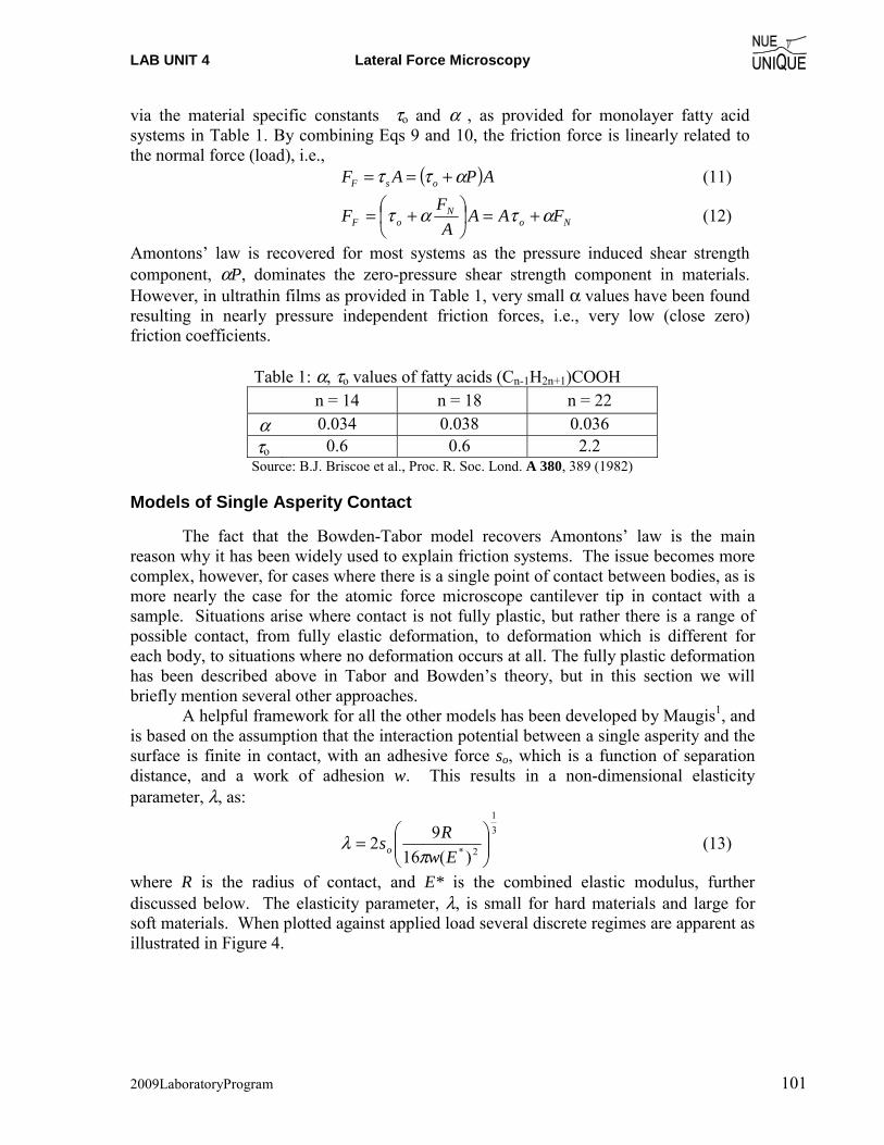
LAB UNIT 4 Lateral Force Microscopy
2009LaboratoryProgram 101
via the material specific constants τo and α , as provided for monolayer fatty acid systems in Table 1. By combining Eqs 9 and 10, the friction force is linearly related to the normal force (load), i.e.,
( )APAF osF αττ +== (11)
NoN
oF FAAA
FF ατατ +=⎟⎠
⎞⎜⎝
⎛ += (12)
Amontons’ law is recovered for most systems as the pressure induced shear strength component, αP, dominates the zero-pressure shear strength component in materials. However, in ultrathin films as provided in Table 1, very small α values have been found resulting in nearly pressure independent friction forces, i.e., very low (close zero) friction coefficients.
Table 1: α, τo values of fatty acids (Cn-1H2n+1)COOH n = 14 n = 18 n = 22 α 0.034 0.038 0.036 τo 0.6 0.6 2.2
Source: B.J. Briscoe et al., Proc. R. Soc. Lond. A 380, 389 (1982)
Models of Single Asperity Contact
The fact that the Bowden-Tabor model recovers Amontons’ law is the main reason why it has been widely used to explain friction systems. The issue becomes more complex, however, for cases where there is a single point of contact between bodies, as is more nearly the case for the atomic force microscope cantilever tip in contact with a sample. Situations arise where contact is not fully plastic, but rather there is a range of possible contact, from fully elastic deformation, to deformation which is different for each body, to situations where no deformation occurs at all. The fully plastic deformation has been described above in Tabor and Bowden’s theory, but in this section we will briefly mention several other approaches. A helpful framework for all the other models has been developed by Maugis1, and is based on the assumption that the interaction potential between a single asperity and the surface is finite in contact, with an adhesive force so, which is a function of separation distance, and a work of adhesion w. This results in a non-dimensional elasticity parameter, λ, as:
31
2* )(1692 ⎟⎟
⎠
⎞⎜⎜⎝
⎛=
EwRso π
λ (13)
where R is the radius of contact, and E* is the combined elastic modulus, further discussed below. The elasticity parameter, λ, is small for hard materials and large for soft materials. When plotted against applied load several discrete regimes are apparent as illustrated in Figure 4.
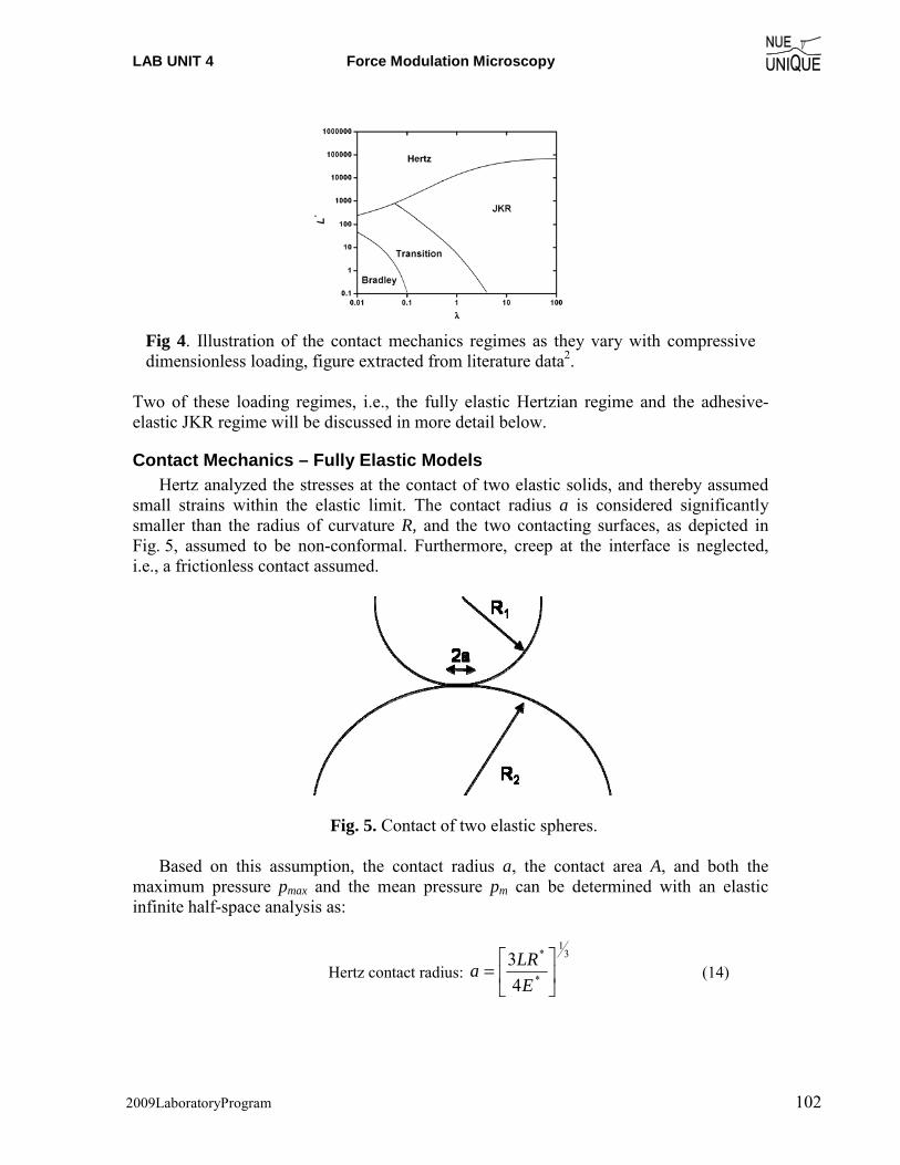
LAB UNIT 4 Force Modulation Microscopy
2009LaboratoryProgram 102
Fig 4. Illustration of the contact mechanics regimes as they vary with compressive dimensionless loading, figure extracted from literature data2.
Two of these loading regimes, i.e., the fully elastic Hertzian regime and the adhesive-elastic JKR regime will be discussed in more detail below.
Contact Mechanics – Fully Elastic Models Hertz analyzed the stresses at the contact of two elastic solids, and thereby assumed
small strains within the elastic limit. The contact radius a is considered significantly smaller than the radius of curvature R, and the two contacting surfaces, as depicted in Fig. 5, assumed to be non-conformal. Furthermore, creep at the interface is neglected, i.e., a frictionless contact assumed.
Fig. 5. Contact of two elastic spheres.
Based on this assumption, the contact radius a, the contact area A, and both the maximum pressure pmax and the mean pressure pm can be determined with an elastic infinite half-space analysis as:
Hertz contact radius: 3
1
*
*
43
⎥⎦
⎤⎢⎣
⎡=
ELRa (14)
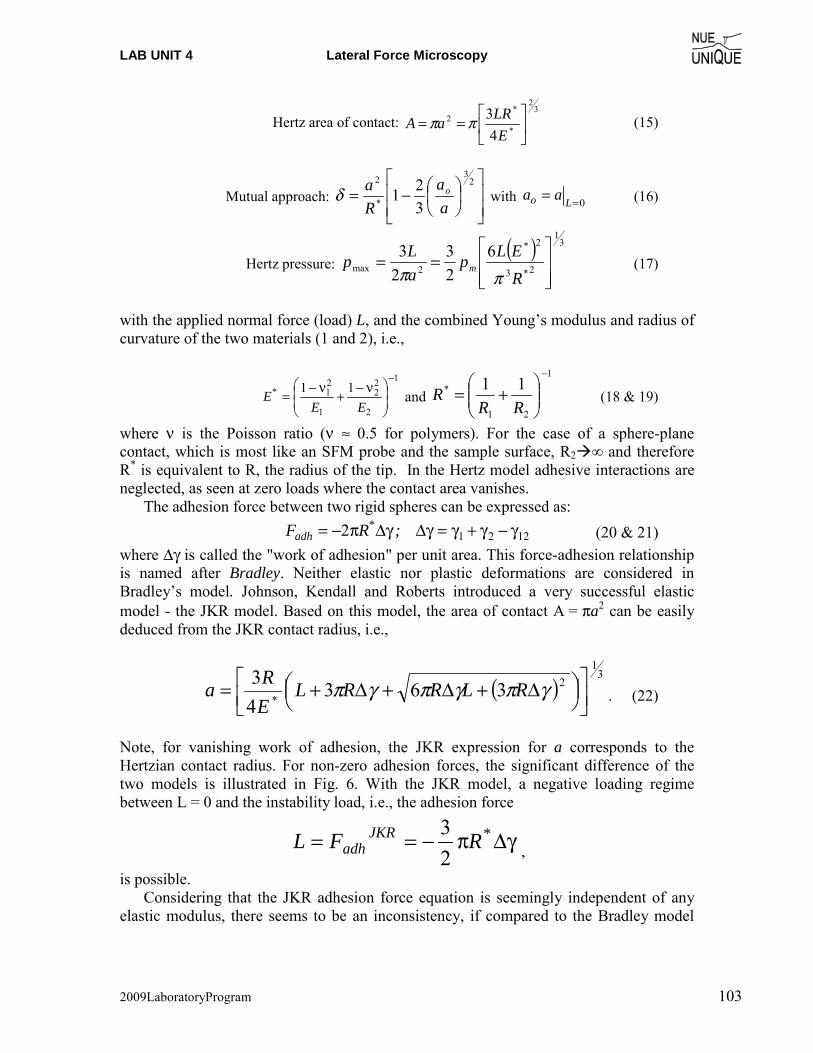
LAB UNIT 4 Lateral Force Microscopy
2009LaboratoryProgram 103
Hertz area of contact: 3
2
*
*2
43
⎥⎦
⎤⎢⎣
⎡==
ELRaA ππ (15)
Mutual approach: ⎥⎥
⎦
⎤
⎢⎢
⎣
⎡⎟⎠
⎞⎜⎝
⎛−=2
3
*
2
321
aa
Ra oδ with 0== Lo aa (16)
Hertz pressure: ( ) 3
1
2*3
2*
2max6
23
23
⎥⎥⎦
⎤
⎢⎢⎣
⎡==
RELp
aLp m
ππ (17)
with the applied normal force (load) L, and the combined Young’s modulus and radius of curvature of the two materials (1 and 2), i.e.,
1
2
22
1
21 11
−
⎟⎟
⎠
⎞
⎜⎜
⎝
⎛ ν−+
ν−=
EEE* and
1
21
* 11−
⎟⎟⎠
⎞⎜⎜⎝
⎛+=
RRR (18 & 19)
where ν is the Poisson ratio (ν ≈ 0.5 for polymers). For the case of a sphere-plane contact, which is most like an SFM probe and the sample surface, R2�∞ and therefore R* is equivalent to R, the radius of the tip. In the Hertz model adhesive interactions are neglected, as seen at zero loads where the contact area vanishes.
The adhesion force between two rigid spheres can be expressed as: 12212 γ−γ+γ=γΔγΔπ−= ;RF *
adh (20 & 21) where Δγ is called the "work of adhesion" per unit area. This force-adhesion relationship is named after Bradley. Neither elastic nor plastic deformations are considered in Bradley’s model. Johnson, Kendall and Roberts introduced a very successful elastic model - the JKR model. Based on this model, the area of contact A = πa2 can be easily deduced from the JKR contact radius, i.e.,
( )3
12
*363
43
⎥⎦
⎤⎢⎣
⎡⎟⎠⎞⎜
⎝⎛ Δ+Δ+Δ+= γπγπγπ RLRRL
ERa . (22)
Note, for vanishing work of adhesion, the JKR expression for a corresponds to the Hertzian contact radius. For non-zero adhesion forces, the significant difference of the two models is illustrated in Fig. 6. With the JKR model, a negative loading regime between L = 0 and the instability load, i.e., the adhesion force
γΔπ−== *JKRadh RFL
23
,
is possible. Considering that the JKR adhesion force equation is seemingly independent of any
elastic modulus, there seems to be an inconsistency, if compared to the Bradley model
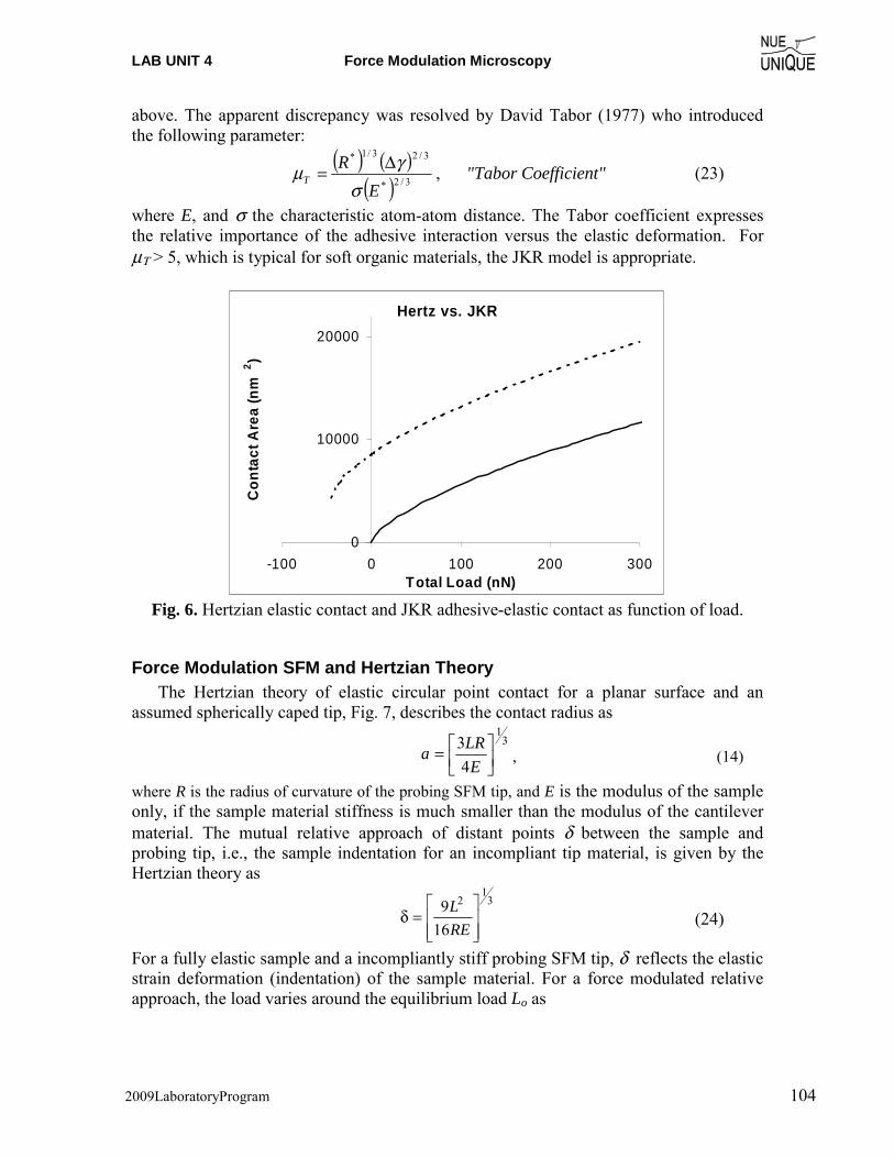
LAB UNIT 4 Force Modulation Microscopy
2009LaboratoryProgram 104
above. The apparent discrepancy was resolved by David Tabor (1977) who introduced the following parameter:
( ) ( )( ) 3/2*
3/23/1*
ER
Tσ
γμ Δ= , "Tabor Coefficient" (23)
where E, and σ the characteristic atom-atom distance. The Tabor coefficient expresses the relative importance of the adhesive interaction versus the elastic deformation. For μΤ > 5, which is typical for soft organic materials, the JKR model is appropriate.
Hertz vs. JKR
0
10000
20000
-100 0 100 200 300Total Load (nN)
Con
tact
Are
a (n
m2 )
Fig. 6. Hertzian elastic contact and JKR adhesive-elastic contact as function of load.
Force Modulation SFM and Hertzian Theory The Hertzian theory of elastic circular point contact for a planar surface and an
assumed spherically caped tip, Fig. 7, describes the contact radius as
3
1
43
⎥⎦
⎤⎢⎣
⎡=E
LRa , (14)
where R is the radius of curvature of the probing SFM tip, and E is the modulus of the sample only, if the sample material stiffness is much smaller than the modulus of the cantilever material. The mutual relative approach of distant points δ between the sample and probing tip, i.e., the sample indentation for an incompliant tip material, is given by the Hertzian theory as
3
12
169
⎥⎥⎦
⎤
⎢⎢⎣
⎡=δ
REL
(24)
For a fully elastic sample and a incompliantly stiff probing SFM tip, δ reflects the elastic strain deformation (indentation) of the sample material. For a force modulated relative approach, the load varies around the equilibrium load Lo as

LAB UNIT 4 Lateral Force Microscopy
2009LaboratoryProgram 105
δδ∂
∂+= LLL o (25)
As we consider only the sample being deformed, a one-dimensional sample stiffness (generally referred to as contact stiffness) can be introduced as the derivative of the load, i.e.,
( ) 3126 RLELk oc =
δ∂∂≡ (26)
The equation above is synonymous with the non-adhesive Hertzian expression aEkc 2= (27) Higher order derivatives provide anharmonic distortions (dissipation) that can be neglected. The equilibrium load can be expressed by the normal spring constant of the cantilever kL and the equilibrium deflection zo as Lo= kL zo .
Fig. 7. Elastic sample deformation involving rigid SFM tip. Thus, for a sinusoidal normal stress disturbance, z = A sin(ωt), with a root mean square amplitude
Az2
1= (28)
the dynamic force acting on the cantilever is proportional to the net displacement (input modulation minus sample deformation), i.e.,
( )δ−=Δ zkF L (29) In an analogous manner the force modulation can also be described from the sample perspective as δ=Δ ckF (30)
The "normal force", ΔF, acting on the SFM lever in the process of an indentation can be expressed in Hooke’s limit as LLcsys zkkzkF Δ=δ==Δ with δ−=Δ zzL , (31) as illustrated in Fig. 7. The system combined spring constant, ksys , is then given as
LAB UNIT 4 Force Modulation Microscopy
2009LaboratoryProgram 106
111
−
⎟⎟⎠
⎞⎜⎜⎝
⎛+=
Lcsys kk
k . (32)
Analogous relationships exist also for elastic shear modulation.
Contact Stiffness In the previous paragraph, we have assumed that only the sample is deformed and the
material response is rate independent. If both bodies are compliant, the non-adhesive Hertzian contact stiffness is given as
*
c aEk 2= (33) where Ei and νi (I = 1,2) are the reduced material Young's moduli and Poisson ratios, respectively. This equation has also been found to be applicable for viscoelastic materials, i.e.,3
( ) ( )ω=ω *c aEk 2 (34)
where kc(ω) and E(ω) reflect effective stiffnesses. If we also consider adhesion to take place in the contact area, the Hertzian theory
would have to be replaced by the JKR theory, which leads to the following expression for a normalized contact stiffness to zero load:3
( )
( )3
2
0 211
⎥⎥⎦
⎤
⎢⎢⎣
⎡ −+=
ωω
=
adh
Lc
c F/Lk
k (35)
( ) ( ) ( )3
1
0
2
0 2922
⎥⎥⎥
⎦
⎤
⎢⎢⎢
⎣
⎡γΔπω=ω=ω
→ω
= ***
oLcE
REEak (36)
Force Modulation and Polymer Relaxation Properties Controlled temperature experiments involving force modulation microscopy provide the opportunity to investigate relaxation properties of polymeric and organic materials. Thereby, the contact stiffness is monitored as a function the temperature, as illustrated below with shear modulation force microscopy (SM-FM) employed to thin polystyrene films. Due to the small probing area even the smallest changes in the polymer internal pressure, modulus and surface energies can be detected. SM-FM is allows for accurate determination of transition properties, such as the glass transition temperature,* Tg, of nanoconstrained systems, such as ultrathin polymer films with a thickness below ~100 nm, Fig. 8(a).
The SM-FM method is briefly described as follows: A nanometer sharp SFM cantilever tip is brought into contact with the sample surface, Fig. 8(b). While a constant load is applied, the probing tip is laterally modulated with a "no-slip" nanometer amplitude, ΔX,IN. The modulation response, ΔXOUT, is analyzed using a two-channel lock-in amplifier, comparing the response signal to the input signal. The modulation response, * Background information regarding the glass transition of viscoelastic material is provided below.
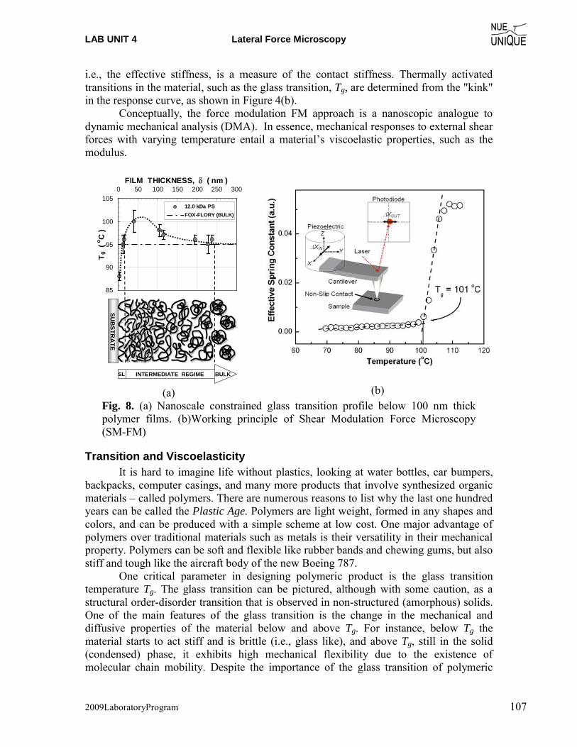
LAB UNIT 4 Lateral Force Microscopy
2009LaboratoryProgram 107
i.e., the effective stiffness, is a measure of the contact stiffness. Thermally activated transitions in the material, such as the glass transition, Tg, are determined from the "kink" in the response curve, as shown in Figure 4(b).
Conceptually, the force modulation FM approach is a nanoscopic analogue to dynamic mechanical analysis (DMA). In essence, mechanical responses to external shear forces with varying temperature entail a material’s viscoelastic properties, such as the modulus.
85
90
95
100
1050 50 100 150 200 250 300
FILM THICKNESS, δ ( nm )
Tg
( o C )
12.0 kDa PSFOX-FLORY (BULK)
SUB
STRA
TE
SL INTERMEDIATE REGIME BULK
(a)
(b) Fig. 8. (a) Nanoscale constrained glass transition profile below 100 nm thick polymer films. (b)Working principle of Shear Modulation Force Microscopy (SM-FM)
Transition and Viscoelasticity It is hard to imagine life without plastics, looking at water bottles, car bumpers,
backpacks, computer casings, and many more products that involve synthesized organic materials – called polymers. There are numerous reasons to list why the last one hundred years can be called the Plastic Age. Polymers are light weight, formed in any shapes and colors, and can be produced with a simple scheme at low cost. One major advantage of polymers over traditional materials such as metals is their versatility in their mechanical property. Polymers can be soft and flexible like rubber bands and chewing gums, but also stiff and tough like the aircraft body of the new Boeing 787.
One critical parameter in designing polymeric product is the glass transition temperature Tg. The glass transition can be pictured, although with some caution, as a structural order-disorder transition that is observed in non-structured (amorphous) solids. One of the main features of the glass transition is the change in the mechanical and diffusive properties of the material below and above Tg. For instance, below Tg the material starts to act stiff and is brittle (i.e., glass like), and above Tg, still in the solid (condensed) phase, it exhibits high mechanical flexibility due to the existence of molecular chain mobility. Despite the importance of the glass transition of polymeric
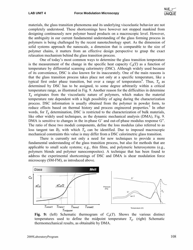
LAB UNIT 4 Force Modulation Microscopy
2009LaboratoryProgram 108
materials, the glass transition phenomena and its underlying viscoelastic behavior are not completely understood. These shortcomings have however not stopped mankind from designing continuously new polymer based products on a macroscopic level. However, the ambiguity in our current fundamental understanding of the glass forming process in polymers is being challenged by the recent nanotechnology spurt. As the dimension of solid systems approach the nanoscale, a dimension that is comparable to the size of polymer chains, it matters from an effective design perspective to grasp the exact relaxation mechanism behind the glass transition process.
One of today’s most common ways to determine the glass transition temperature is the measurement of the change in the specific heat capacity Cp(T) as a function of temperature by differential scanning calorimetry (DSC). Although widely used because of its convenience, DSC is also known for its inaccurately. One of the main reasons is that the glass transition process takes place not only at a specific temperature, like a typical first order phase transition, but over a range of temperatures4. Thus, Tg as determined by DSC has to be assigned, to some degree arbitrarily within a critical temperature range, as illustrated in Fig. 9. Another reason for the difficulties in determine Tg originates from the viscoelastic nature of polymers, which makes the material temperature rate dependent with a high possibility of aging during the characterization process. DSC information is usually obtained from the polymer in powder form, to reduce effects based on thermal history and process engineered properties.5 In other words, for Tg determination, DSC is restricted to the characterization of bulk materials, like other widely used techniques, as the dynamic mechanical analysis (DMA), Fig. 9. DMA is sensitive to changes in the in-phase G’ and out-of-phase modulus response G”. The ratio of these two moduli components, define the loss modulus (also referred to as loss tangent tan δ), with which Tg can be identified. Due to imposed macroscopic mechanical constraints this value is may differ from a DSC calorimetric glass transition.
There is currently not only a need for new techniques to provide a more fundamental understanding of the glass transition process, but also for methods that are applicable to small scale systems; e.g., thin films, and polymeric heterosystems (e.g., polymers blends and polymer nanocomposites). A technique that has been found to address the experimental shortcomings of DSC and DMA is shear modulation force microscopy (SM-FM), as introduced above.
Temperature (K)
Pressure(Pa)
tan
G’’
G’’
Fig. 9: (left) Schematic thermogram of Cp(T). Shows the various distinct temperatures used to define the midpoint temperature Tg. (right) Schematic thermomechanical results, as obtainable by DMA.
Tg
LAB UNIT 4 Lateral Force Microscopy
2009LaboratoryProgram 109
Introduction to Linear Viscoelasticity The science that deals with the mechanical properties of condensed phases under
external stresses is called Rheology. We will limit our discussion to a subdiscipline of rheology, i.e., linear viscoelasticity, with which we conceptually separate the liquid-like (viscous) behavior from the solid-like (elastic) behavior. Thereby, a material that exhibits ideal solid-like behavior under stress can be described with a simple stress-strain relationship, and a material with ideal liquid-like behavior shows a simple stress-strain-rate dependence. With stress we define the external force per unit area that is imposed on the condensed phase. The resulting deformation (e.g., length or angular deformation (ΔL or γ) for a uniaxial length extension, or simple shear, respectively) defines a strain ratio (e.g., (Lo+ΔL)/Lo or tan γ). It is convention to use for uniaxial stress and strain the Greek symbols σ and ε and for the shear stress and strain τ and γ. Strain rates reflect the time derivative of the strain.
Ideal solid-like and ideal liquid-like
Ideal solid-like materials deform and relax instantaneously with changes in the applied external stresses. Hooke's Law, mentioned above, is a manifestation of a solid-like behavior. Thus, an ideal solid-like behavior is synonymous with ideal elastic. Mechanical energy is stored in an ideal elastic material without exhibiting any form of energy dissipation. The energy is instantaneously regained with the discharge of the external stresses. The conceptual counter behavior to ideal solid-like is ideal liquid-like as found in a Newtonian liquid. The basic equation of simple flow is described one-dimensionally by Newton’s law of viscosity,
dydvx
yx η−=τ , (37)
which relates proportionally the shear force per unit area, Fx/A = τxy, to the negative of the local velocity gradient (time derivative of the deformation) with a constant viscosity value, η. The velocity gradient represents a strain rate. If a stress is applied to a Newtonian liquid no strain is built up. The material is incapable of mechanical energy storage. Once the stress is removed the material does not relax. The material resistance to shear manifests itself in the rate with which the stress is imposed. In a perfect liquid we find a linear relationship between the stress and the strain rate. The proportionality factor is called viscosity.
In general, any realistic liquid and solid matter will behave in a mixed manner, solid-like and liquid-like, depending on the degree and time scale over which external stresses are acting.
Linear Viscoelasticity
Mixed liquid-like and solid-like characteristics of viscoelastic materials suggest that the external forces applied are partially stored and partially dissipated. This is nicely described by a simple constitutive equation based on a periodic deformation process. If the viscoelastic behavior is in a linear region, a shear sinusoidal stress that is applied to a viscoelastic body exhibits a sinusoidal strain with a phase lag that is expressed as follows:
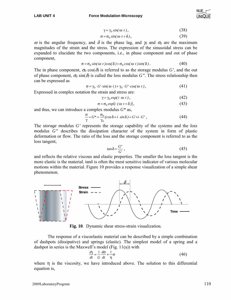
LAB UNIT 4 Force Modulation Microscopy
2009LaboratoryProgram 110
)tsin( ⋅ωγ=γ 0 , (38) )tsin( δ+⋅ωσ=σ 0 , (39) ω is the angular frequency, and δ is the phase lag, and γ0 and σ0 are the maximum magnitudes of the strain and the stress. The expression of the sinusoidal stress can be expanded to elucidate the two components, i.e., in phase component and out of phase component, )sin()tcos()cos()tsin( δ⋅ωσ+δ⋅ωσ=σ 00 . (40) The in phase component, σ0 cos(δ) is referred to as the storage modulus G’, and the out of phase component, σ0 sin(δ) is called the loss modulus G”. The stress relationship then can be expressed as )tcos("G)tsin('G ⋅ω⋅⋅γ+⋅ω⋅⋅γ=σ 00 , (41) Expressed in complex notation the strain and stress are: )tiexp( ⋅ω⋅γ=γ 0 , (42) ( ))t(iexp δ+⋅ω⋅σ=σ 0 , (43) and thus, we can introduce a complex modulus G* as, "Gi'G)sini(cos*G ⋅+=δ⋅+δ
γσ==
γσ
0
0 , (44)
The storage modulus G’ represents the storage capability of the systems and the loss modulus G” describes the dissipation character of the system in form of plastic deformation or flow. The ratio of the loss and the storage component is referred to as the loss tangent,
'G"Gtan =δ , (45)
and reflects the relative viscous and elastic properties. The smaller the loss tangent is the more elastic is the material. tanδ is often the most sensitive indicator of various molecular motions within the material. Figure 10 provides a response visualization of a simple shear phenomenon.
Fig. 10. Dynamic shear stress-strain visualization.
The response of a viscoelastic material can be described by a simple combination
of dashpots (dissipative) and springs (elastic). The simplest model of a spring and a dashpot in series is the Maxwell’s model (Fig. 11(a)) with
ση
+σ=γ 11dtd
Gdtd (46)
where η is the viscosity, we have introduced above. The solution to this differential equation is,
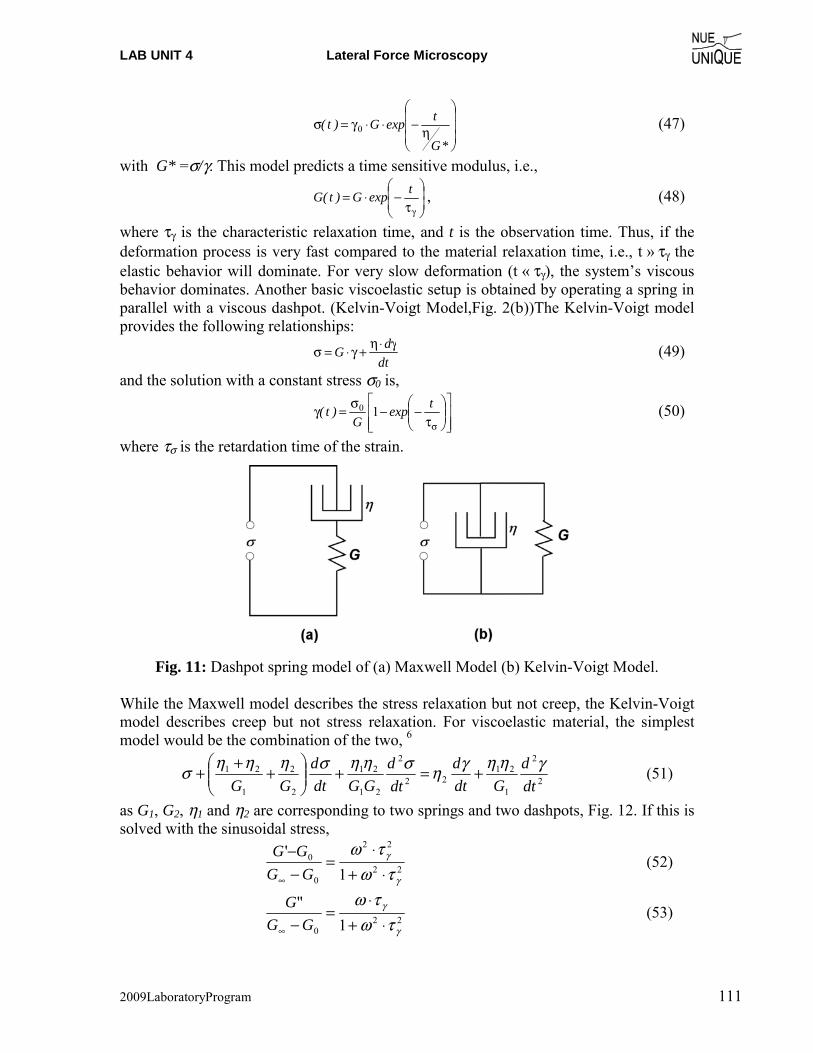
LAB UNIT 4 Lateral Force Microscopy
2009LaboratoryProgram 111
⎟⎟⎟
⎠
⎞
⎜⎜⎜
⎝
⎛
η−⋅⋅γ=σ*G
texpG)t( 0 (47)
with G* =σ/γ. This model predicts a time sensitive modulus, i.e.,
⎟⎟
⎠
⎞
⎜⎜
⎝
⎛
τ−⋅=
γ
texpG)t(G , (48)
where τγ is the characteristic relaxation time, and t is the observation time. Thus, if the deformation process is very fast compared to the material relaxation time, i.e., t » τγ the elastic behavior will dominate. For very slow deformation (t « τγ), the system’s viscous behavior dominates. Another basic viscoelastic setup is obtained by operating a spring in parallel with a viscous dashpot. (Kelvin-Voigt Model,Fig. 2(b))The Kelvin-Voigt model provides the following relationships:
dtdG γ⋅η+γ⋅=σ (49)
and the solution with a constant stress σ0 is,
⎥⎥⎦
⎤
⎢⎢⎣
⎡⎟⎟⎠
⎞⎜⎜⎝
⎛
τ−−σ=γ
σ
texpG
)t( 10 (50)
where τσ is the retardation time of the strain.
Fig. 11: Dashpot spring model of (a) Maxwell Model (b) Kelvin-Voigt Model.
While the Maxwell model describes the stress relaxation but not creep, the Kelvin-Voigt model describes creep but not stress relaxation. For viscoelastic material, the simplest model would be the combination of the two, 6
2
2
1
2122
2
21
21
2
2
1
21
dtd
Gdtd
dtd
GGdtd
GGγηηγησηησηηησ +=+⎟⎟
⎠
⎞⎜⎜⎝
⎛+
++ (51)
as G1, G2, η1 and η2 are corresponding to two springs and two dashpots, Fig. 12. If this is solved with the sinusoidal stress,
22
22
0
0
1'
γ
γ
τωτω⋅+
⋅=
−−
∞ GGGG
(52)
220 1
"
γ
γ
τωτω
⋅+⋅
=−∞ GG
G (53)
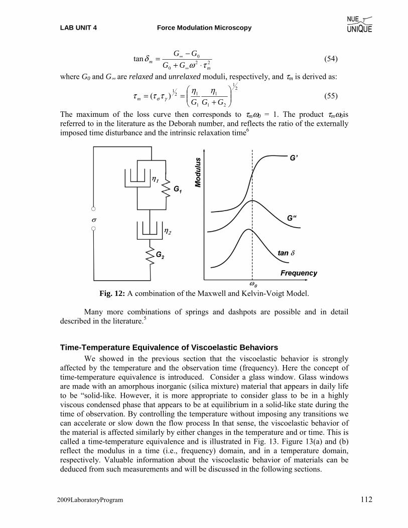
LAB UNIT 4 Force Modulation Microscopy
2009LaboratoryProgram 112
220
0tanm
m GGGG
τωδ
⋅+−
=∞
∞ (54)
where G0 and G∞ are relaxed and unrelaxed moduli, respectively, and τm is derived as:
2
1
21
1
1
121
)( ⎟⎟⎠
⎞⎜⎜⎝
⎛
+==
GGGmηητττ γσ (55)
The maximum of the loss curve then corresponds to τmω0 = 1. The product τmω0is referred to in the literature as the Deborah number, and reflects the ratio of the externally imposed time disturbance and the intrinsic relaxation time6
Fig. 12: A combination of the Maxwell and Kelvin-Voigt Model.
Many more combinations of springs and dashpots are possible and in detail
described in the literature.5
Time-Temperature Equivalence of Viscoelastic Behaviors We showed in the previous section that the viscoelastic behavior is strongly
affected by the temperature and the observation time (frequency). Here the concept of time-temperature equivalence is introduced. Consider a glass window. Glass windows are made with an amorphous inorganic (silica mixture) material that appears in daily life to be “solid-like. However, it is more appropriate to consider glass to be in a highly viscous condensed phase that appears to be at equilibrium in a solid-like state during the time of observation. By controlling the temperature without imposing any transitions we can accelerate or slow down the flow process In that sense, the viscoelastic behavior of the material is affected similarly by either changes in the temperature and or time. This is called a time-temperature equivalence and is illustrated in Fig. 13. Figure 13(a) and (b) reflect the modulus in a time (i.e., frequency) domain, and in a temperature domain, respectively. Valuable information about the viscoelastic behavior of materials can be deduced from such measurements and will be discussed in the following sections.
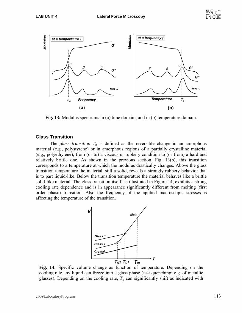
LAB UNIT 4 Lateral Force Microscopy
2009LaboratoryProgram 113
Fig. 13: Modulus spectrums in (a) time domain, and in (b) temperature domain.
Glass Transition The glass transition Tg is defined as the reversible change in an amorphous material (e.g., polystyrene) or in amorphous regions of a partially crystalline material (e.g., polyethylene), from (or to) a viscous or rubbery condition to (or from) a hard and relatively brittle one. As shown in the previous section, Fig. 13(b), this transition corresponds to a temperature at which the modulus drastically changes. Above the glass transition temperature the material, still a solid, reveals a strongly rubbery behavior that is to part liquid-like. Below the transition temperature the material behaves like a brittle solid-like material. The glass transition itself, as illustrated in Figure 14, exhibits a strong cooling rate dependence and is in appearance significantly different from melting (first order phase) transition. Also the frequency of the applied macroscopic stresses is affecting the temperature of the transition.
Fig. 14: Specific volume change as function of temperature. Depending on the cooling rate any liquid can freeze into a glass phase (fast quenching; e.g. of metallic glasses). Depending on the cooling rate, Tg can significantly shift as indicated with
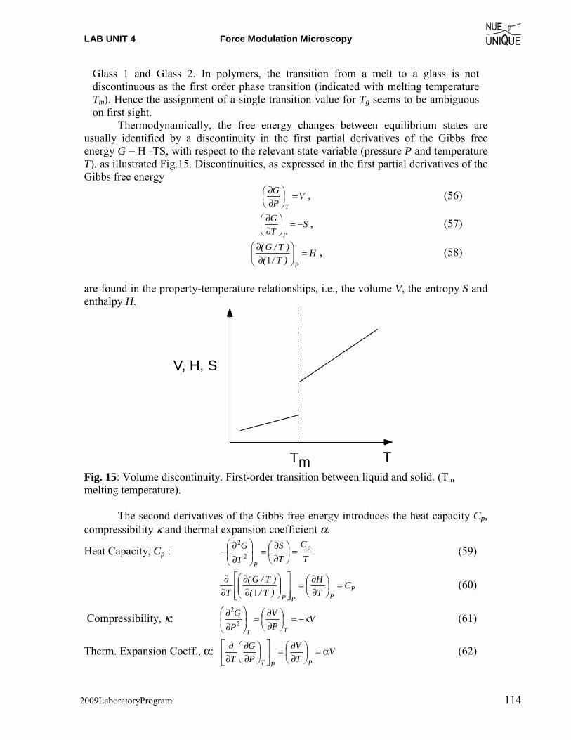
LAB UNIT 4 Force Modulation Microscopy
2009LaboratoryProgram 114
Glass 1 and Glass 2. In polymers, the transition from a melt to a glass is not discontinuous as the first order phase transition (indicated with melting temperature Tm). Hence the assignment of a single transition value for Tg seems to be ambiguous on first sight.
Thermodynamically, the free energy changes between equilibrium states are usually identified by a discontinuity in the first partial derivatives of the Gibbs free energy G = H -TS, with respect to the relevant state variable (pressure P and temperature T), as illustrated Fig.15. Discontinuities, as expressed in the first partial derivatives of the Gibbs free energy
VPG
T=⎟
⎠
⎞⎜⎝
⎛
∂∂ , (56)
STG
P−=⎟
⎠
⎞⎜⎝
⎛
∂∂ , (57)
H)T/()T/G(
P=⎟⎟
⎠
⎞⎜⎜⎝
⎛
∂∂
1, (58)
are found in the property-temperature relationships, i.e., the volume V, the entropy S and enthalpy H.
V, H, S
Tm T
Fig. 15: Volume discontinuity. First-order transition between liquid and solid. (Tm melting temperature).
The second derivatives of the Gibbs free energy introduces the heat capacity Cp,
compressibility κ and thermal expansion coefficient α.
Heat Capacity, Cp : TC
TS
TG p
P
=⎟⎠
⎞⎜⎝
⎛
∂∂=
⎟⎟
⎠
⎞
⎜⎜
⎝
⎛
∂∂− 2
2 (59)
PPPP
CTH
)T/()T/G(
T=⎟
⎠
⎞⎜⎝
⎛
∂∂=
⎥⎥⎦
⎤
⎢⎢⎣
⎡⎟⎟⎠
⎞⎜⎜⎝
⎛
∂∂
∂∂
1 (60)
Compressibility, κ: VPV
PG
TT
κ−=⎟⎠
⎞⎜⎝
⎛
∂∂=
⎟⎟
⎠
⎞
⎜⎜
⎝
⎛
∂∂
2
2 (61)
Therm. Expansion Coeff., α: VTV
PG
T PPTα=⎟
⎠
⎞⎜⎝
⎛
∂∂=⎥
⎦
⎤⎢⎣
⎡⎟⎠
⎞⎜⎝
⎛
∂∂
∂∂ (62)
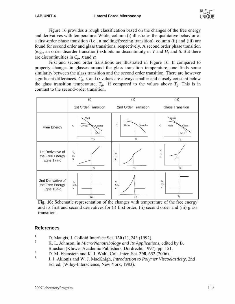
LAB UNIT 4 Lateral Force Microscopy
2009LaboratoryProgram 115
Figure 16 provides a rough classification based on the changes of the free energy and derivatives with temperature. While, column (i) illustrates the qualitative behavior of a first-order phase transition (i.e., a melting/freezing transition), column (ii) and (iii) are found for second order and glass transitions, respectively. A second order phase transition (e.g., an order-disorder transition) exhibits no discontinuity in V and H, and S. But there are discontinuities in Cp, κ and α.
First and second order transitions are illustrated in Figure 16. If compared to property changes in glasses around the glass transition temperature, one finds some similarity between the glass transition and the second order transition. There are however significant differences. Cp, κ and α values are always smaller and closely constant below the glass transition temperature, Tg, if compared to the values above Tg. This is in contrast to the second-order transition.
(i) (ii) (iii)
1st Order Transition 2nd Order Transition Glass Transition
Free Energy
1st Derivative of the Free Energy
Eqns 17a-c
2nd Derivative of the Free Energy
Eqns 18a-c
Tg
Melt GlassG
Melt
Glass
Tm
G
Melt
Crystal
Melt
Crystal
Tc
Order DisorderG
Tm
V,H,S
Tc
V,H,S
Tg
V,H,S
Tm
α,Cp,κ
Tc
α,Cp,κ
Tg
α,Cp,κ
Fig. 16: Schematic representation of the changes with temperature of the free energy and its first and second derivatives for (i) first order, (ii) second order and (iii) glass transition.
References 1 D. Maugis, J. Colloid Interface Sci. 150 (1), 243 (1992). 2 K. L. Johnson, in Micro/Nanotribology and Its Applications, edited by B.
Bhushan (Kluwer Academic Publishers, Dordrecht, 1997), pp. 151. 3 D. M. Ebenstein and K. J. Wahl, Coll. Inter. Sci. 298, 652 (2006). 4 J. J. Aklonis and W. J. MacKnigh, Introduction to Polymer Viscoelasticity, 2nd
Ed. ed. (Wiley-Interscience, New York, 1983).
LAB UNIT 4 Force Modulation Microscopy
2009LaboratoryProgram 116
5 D. W. Van Krevelen, Properties of Polymers. (Elsevier Scientific Publishing Company, Amsterdam, 1976).
6 P. Hedvig, Dielectric Spectroscopy of Polymers. (John Wiley & Sons, New York, 1977).
Recommended Reading
Introduction to Polymer Viscoelasticity by John J. Alkonis and William J. MacKnight, Wiley-Interscience Publication, 2nd Ed., New York, 1983.
Mechanical Properties of Solid Polymers by I. M. Ward, Wiley-Interscience Publication, London, 1971. Nanoscience: Friction and Rheology on the Nanometer Scale by E. Meyer, R. M. Overney, K. Dransfeld,
and T. Gyalog, World Scientific Publ., Singapore, 1998.
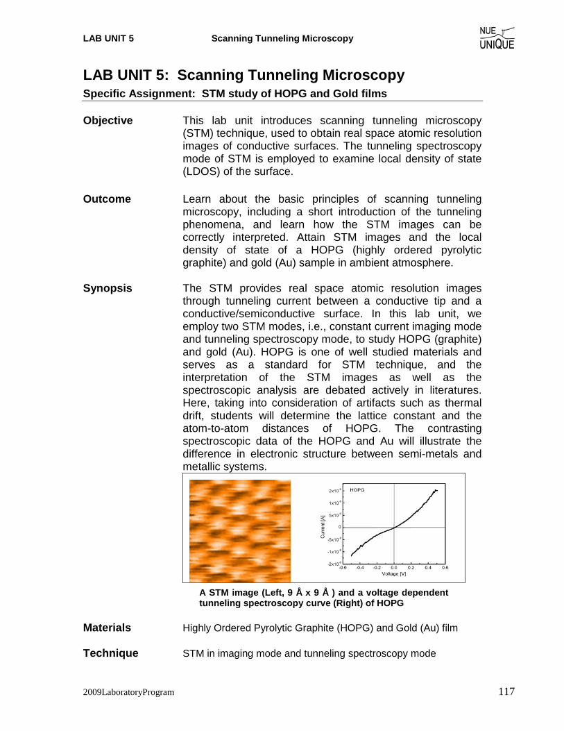
LAB UNIT 5 Scanning Tunneling Microscopy
2009LaboratoryProgram 117
LAB UNIT 5: Scanning Tunneling Microscopy Specific Assignment: STM study of HOPG and Gold films Objective This lab unit introduces scanning tunneling microscopy
(STM) technique, used to obtain real space atomic resolution images of conductive surfaces. The tunneling spectroscopy mode of STM is employed to examine local density of state (LDOS) of the surface.
Outcome Learn about the basic principles of scanning tunneling
microscopy, including a short introduction of the tunneling phenomena, and learn how the STM images can be correctly interpreted. Attain STM images and the local density of state of a HOPG (highly ordered pyrolytic graphite) and gold (Au) sample in ambient atmosphere.
Synopsis The STM provides real space atomic resolution images
through tunneling current between a conductive tip and a conductive/semiconductive surface. In this lab unit, we employ two STM modes, i.e., constant current imaging mode and tunneling spectroscopy mode, to study HOPG (graphite) and gold (Au). HOPG is one of well studied materials and serves as a standard for STM technique, and the interpretation of the STM images as well as the spectroscopic analysis are debated actively in literatures. Here, taking into consideration of artifacts such as thermal drift, students will determine the lattice constant and the atom-to-atom distances of HOPG. The contrasting spectroscopic data of the HOPG and Au will illustrate the difference in electronic structure between semi-metals and metallic systems.
A STM image (Left, 9 Å x 9 Å ) and a voltage dependent tunneling spectroscopy curve (Right) of HOPG
Materials Highly Ordered Pyrolytic Graphite (HOPG) and Gold (Au) film Technique STM in imaging mode and tunneling spectroscopy mode

LAB UNIT 5 Scanning Tunneling Microscopy
2009LaboratoryProgram 118
Table of Contents 1. Assignment................................................................................................. 119 2. Quiz – Preparation for the Experiment..................................................... 120
Theoretical Questions.............................................................................................. 120 Prelab Quiz .............................................................................................................. 120
3. Experimental Assignment ......................................................................... 121 Goal ......................................................................................................................... 121 Safety....................................................................................................................... 121 Instrumental Setup................................................................................................... 121 Materials.................................................................................................................. 121 Experimental Procedure .......................................................................................... 121
4. Background: Local Electronic Properties and STM................................ 127 Motivation ............................................................................................................... 127 Scanning Tunneling Microscopy ............................................................................ 127 Tunneling Spectroscopy.......................................................................................... 131 Layered Structure of HOPG.................................................................................... 133 References ............................................................................................................... 134 Recommended Reading........................................................................................... 134
LAB UNIT 5 Scanning Tunneling Microscopy
2009LaboratoryProgram 119
1. Assignment The assignment is to study the layered structure of HOPG and Au films. Specifically, the lattice constant and the atom-to-atom distances of HOPG will be determined from the STM images. Conductivity, i.e., band structure, of HOPG and Au are also discussed by analyzing the tunneling spectroscopy data. The steps are outlined here:
1. Familiarize yourself with the background information provided in Section 4. 2. Test your background knowledge with the provided Quiz in Section 2. 3. Conduct the STM experiments in Section 3. Follow the experimental step-by-step
procedure. 4. Process images and analyze the spectroscopy data as described in Section 3 5. Finally, provide a report with the following information:
(i) Result section: In this section you show your data and discuss instrumental details (i.e., limitations) and the quality of your data (error analysis).
(ii) Discussion section: In this section you discuss and analyze your data in the light of the provided background information.
It is also appropriate to discuss section (i) and (ii) together. (iii) Summery and outlook: Here you summarize your findings and provide an
outlook on how one could proceed. The report is evaluated based on the quality of the discussion and the integration of your experimental data and the provided theory. You are encouraged to discuss results that are unexpected. It is important to include discussions on the causes for discrepancies and inconsistencies in the data.
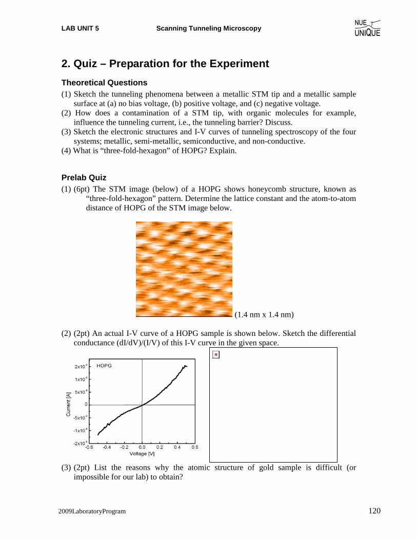
LAB UNIT 5 Scanning Tunneling Microscopy
2009LaboratoryProgram 120
2. Quiz – Preparation for the Experiment Theoretical Questions (1) Sketch the tunneling phenomena between a metallic STM tip and a metallic sample
surface at (a) no bias voltage, (b) positive voltage, and (c) negative voltage. (2) How does a contamination of a STM tip, with organic molecules for example,
influence the tunneling current, i.e., the tunneling barrier? Discuss. (3) Sketch the electronic structures and I-V curves of tunneling spectroscopy of the four
systems; metallic, semi-metallic, semiconductive, and non-conductive. (4) What is “three-fold-hexagon” of HOPG? Explain.
Prelab Quiz (1) (6pt) The STM image (below) of a HOPG shows honeycomb structure, known as
“three-fold-hexagon” pattern. Determine the lattice constant and the atom-to-atom distance of HOPG of the STM image below.
(1.4 nm x 1.4 nm)
(2) (2pt) An actual I-V curve of a HOPG sample is shown below. Sketch the differential conductance (dI/dV)/(I/V) of this I-V curve in the given space.
(3) (2pt) List the reasons why the atomic structure of gold sample is difficult (or
impossible for our lab) to obtain?
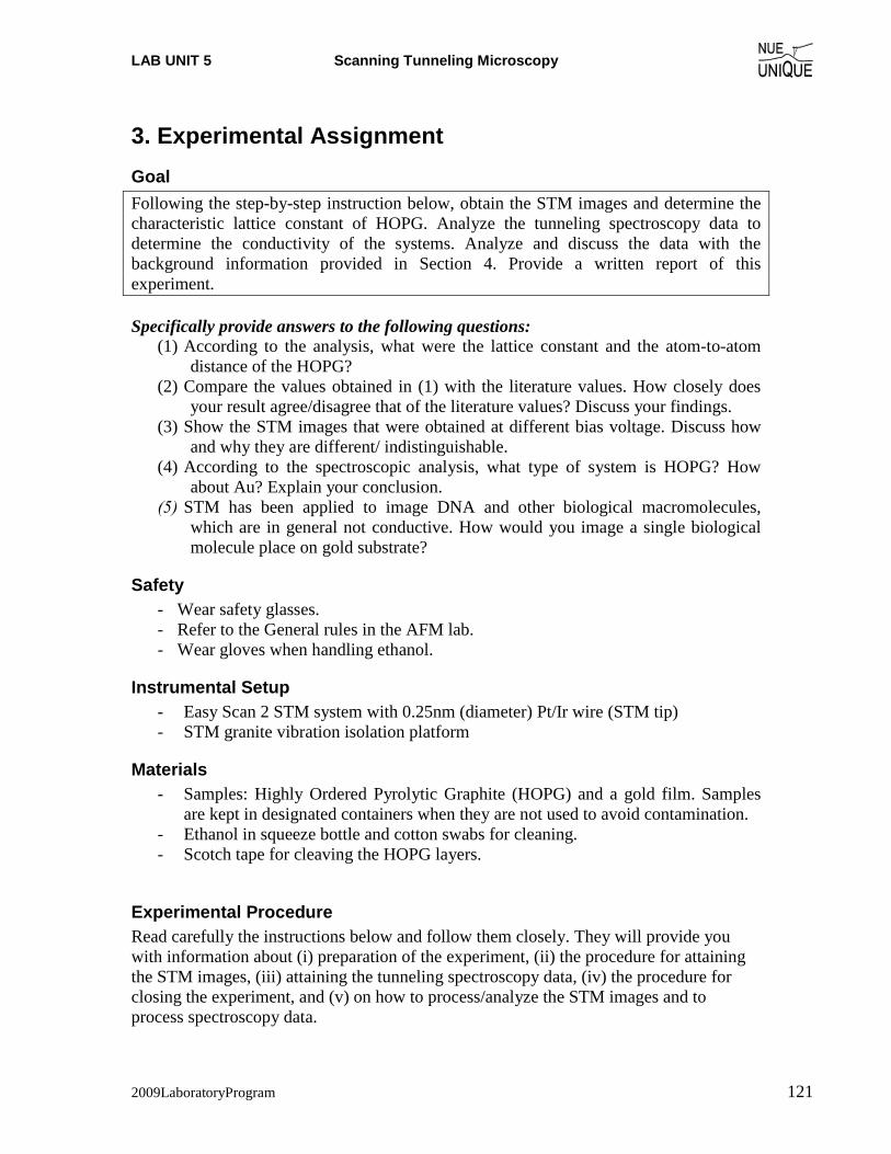
LAB UNIT 5 Scanning Tunneling Microscopy
2009LaboratoryProgram 121
3. Experimental Assignment Goal Following the step-by-step instruction below, obtain the STM images and determine the characteristic lattice constant of HOPG. Analyze the tunneling spectroscopy data to determine the conductivity of the systems. Analyze and discuss the data with the background information provided in Section 4. Provide a written report of this experiment. Specifically provide answers to the following questions:
(1) According to the analysis, what were the lattice constant and the atom-to-atom distance of the HOPG?
(2) Compare the values obtained in (1) with the literature values. How closely does your result agree/disagree that of the literature values? Discuss your findings.
(3) Show the STM images that were obtained at different bias voltage. Discuss how and why they are different/ indistinguishable.
(4) According to the spectroscopic analysis, what type of system is HOPG? How about Au? Explain your conclusion.
(5) STM has been applied to image DNA and other biological macromolecules, which are in general not conductive. How would you image a single biological molecule place on gold substrate?
Safety - Wear safety glasses. - Refer to the General rules in the AFM lab. - Wear gloves when handling ethanol.
Instrumental Setup - Easy Scan 2 STM system with 0.25nm (diameter) Pt/Ir wire (STM tip) - STM granite vibration isolation platform
Materials - Samples: Highly Ordered Pyrolytic Graphite (HOPG) and a gold film. Samples
are kept in designated containers when they are not used to avoid contamination. - Ethanol in squeeze bottle and cotton swabs for cleaning. - Scotch tape for cleaving the HOPG layers.
Experimental Procedure Read carefully the instructions below and follow them closely. They will provide you with information about (i) preparation of the experiment, (ii) the procedure for attaining the STM images, (iii) attaining the tunneling spectroscopy data, (iv) the procedure for closing the experiment, and (v) on how to process/analyze the STM images and to process spectroscopy data.
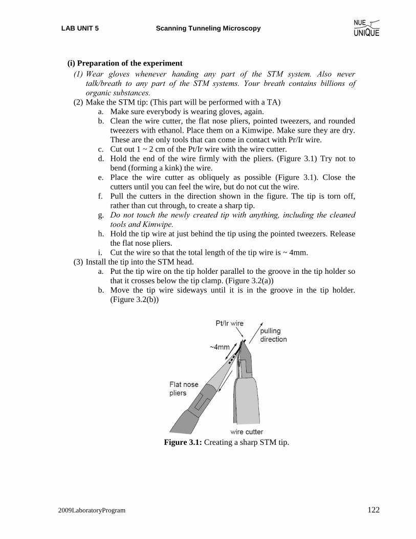
LAB UNIT 5 Scanning Tunneling Microscopy
2009LaboratoryProgram 122
(i) Preparation of the experiment
(1) Wear gloves whenever handing any part of the STM system. Also never talk/breath to any part of the STM systems. Your breath contains billions of organic substances.
(2) Make the STM tip: (This part will be performed with a TA) a. Make sure everybody is wearing gloves, again. b. Clean the wire cutter, the flat nose pliers, pointed tweezers, and rounded
tweezers with ethanol. Place them on a Kimwipe. Make sure they are dry. These are the only tools that can come in contact with Pr/Ir wire.
c. Cut out 1 ~ 2 cm of the Pt/Ir wire with the wire cutter. d. Hold the end of the wire firmly with the pliers. (Figure 3.1) Try not to
bend (forming a kink) the wire. e. Place the wire cutter as obliquely as possible (Figure 3.1). Close the
cutters until you can feel the wire, but do not cut the wire. f. Pull the cutters in the direction shown in the figure. The tip is torn off,
rather than cut through, to create a sharp tip. g. Do not touch the newly created tip with anything, including the cleaned
tools and Kimwipe. h. Hold the tip wire at just behind the tip using the pointed tweezers. Release
the flat nose pliers. i. Cut the wire so that the total length of the tip wire is ~ 4mm.
(3) Install the tip into the STM head. a. Put the tip wire on the tip holder parallel to the groove in the tip holder so
that it crosses below the tip clamp. (Figure 3.2(a)) b. Move the tip wire sideways until it is in the groove in the tip holder.
(Figure 3.2(b))
Figure 3.1: Creating a sharp STM tip.
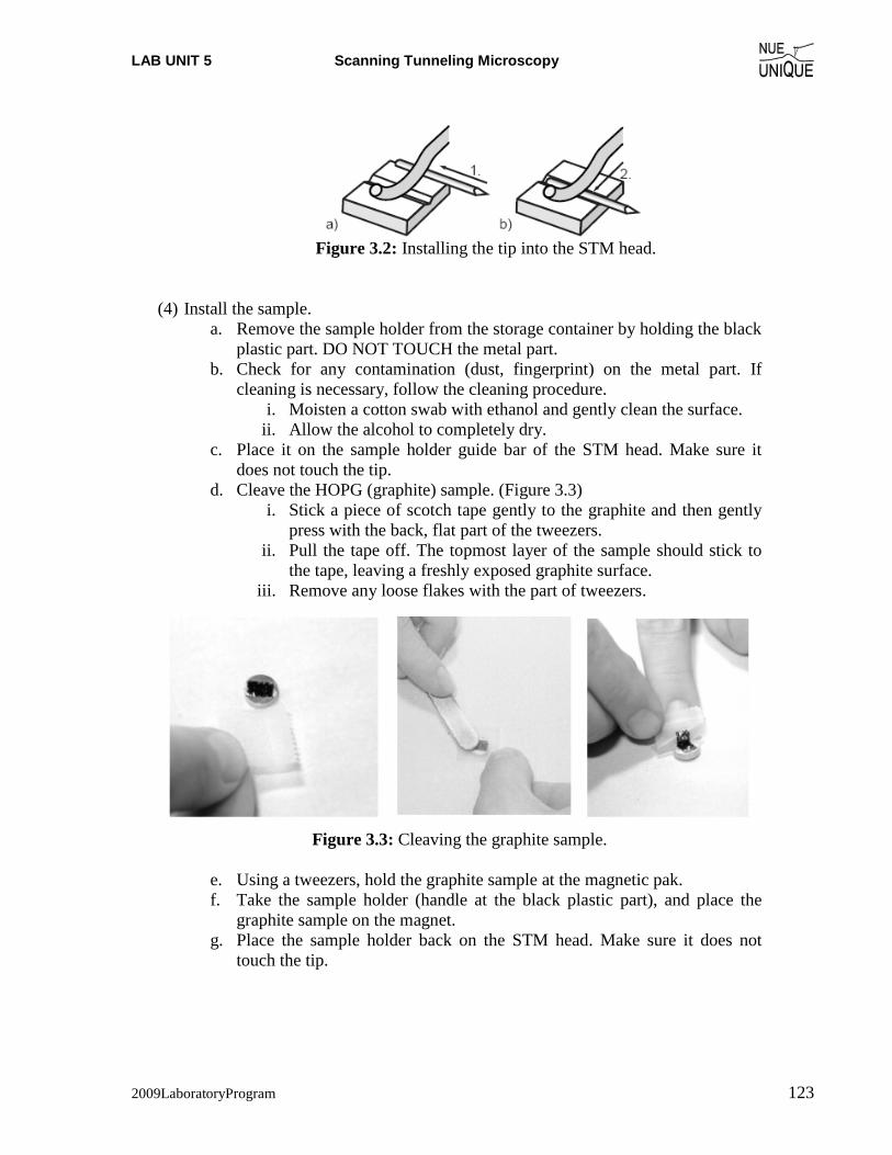
LAB UNIT 5 Scanning Tunneling Microscopy
2009LaboratoryProgram 123
Figure 3.2: Installing the tip into the STM head.
(4) Install the sample. a. Remove the sample holder from the storage container by holding the black
plastic part. DO NOT TOUCH the metal part. b. Check for any contamination (dust, fingerprint) on the metal part. If
cleaning is necessary, follow the cleaning procedure. i. Moisten a cotton swab with ethanol and gently clean the surface.
ii. Allow the alcohol to completely dry. c. Place it on the sample holder guide bar of the STM head. Make sure it
does not touch the tip. d. Cleave the HOPG (graphite) sample. (Figure 3.3)
i. Stick a piece of scotch tape gently to the graphite and then gently press with the back, flat part of the tweezers.
ii. Pull the tape off. The topmost layer of the sample should stick to the tape, leaving a freshly exposed graphite surface.
iii. Remove any loose flakes with the part of tweezers.
Figure 3.3: Cleaving the graphite sample.
e. Using a tweezers, hold the graphite sample at the magnetic pak. f. Take the sample holder (handle at the black plastic part), and place the
graphite sample on the magnet. g. Place the sample holder back on the STM head. Make sure it does not
touch the tip.

LAB UNIT 5 Scanning Tunneling Microscopy
2009LaboratoryProgram 124
Figure 3.4: Placing the sample on the sample holder.
(5) Turn on the Controller main power switch. (6) Open the Easy Scan 2 control software. (7) In the operation mode panel, select STM.
(ii) Procedure for attaining the STM images
(1) Coming in contact. a. Push the sample holder carefully to within 1mm of the tip. The tip should
not touch the sample. b. Look into the graphite surface. There should be a small gap between the
very end of the tip and the reflection of the end of the tip.
Figure 3.5: Coarse approach.
c. Open the Positioning window. d. Through the magnifier, watch the distance between the tip and sample as
click Advance in the approach panel. The tip should be within a fraction of a millimeter to the surface (i.e., the reflection of the tip).
e. Set control parameters in Z-control panel: Set point 1nA, P-gain 10000, I-gain 1000, Tip voltage 50 mV.
f. Click Approach.

LAB UNIT 5 Scanning Tunneling Microscopy
2009LaboratoryProgram 125
g. If the approach was finished successfully, the probe status light changes from blinking to green and automatically start to scan. If not, retract and try again.
(2) Adjust imaging parameters (scan speed, scan direction, tilt, P-gain and I-gain) as the same manner as for AFM imaging. Set the resolution to 256. For attaining atomic resolution,
a. For STM, faster scan speed is better for reducing the thermal drift. b. Image ~ 500 nm area to find a flat location. Zoom into the flat area. c. The atomic resolution images will be ~ 4nm scan size. d. If the image does not show atomic features, try different scan direction,
reduce the gains. e. If none of above work, come out of contact, re-approach. Consult your
teaching assistants for further suggestions. (3) For storing images click Photo in the imaging window. Name files accordingly. (4) Take images at the bias voltage (tip voltage) of 50mV, 250 mV, -50 mV, and -250
mV. Take at least two STM images for each bias voltage.
(iii) Attain the tunneling spectroscopy data
(1) Stop scanning. (2) Open the spectroscopy window. (3) Set parameters: Modulated output is tip voltage, start value -0.5V, end value 0.5
V, modulation time 1s, data point 128, and average 1. (4) Reset the Z-control parameters in z-control window: set-point 1nA and voltage
50mV. (5) Click +Point, and select a location in the image. Click Start. (6) The obtained I-V curve will appear as a dual line graph. (7) Save the curve.
a. Click the I-V curve. b. Click Photo from the imaging window tool bar. The STM image and I-V
curve appears as a separate window. c. From File, select Export, current chart as…, (X, Y, Z)-Points (*csv).
Name accordingly. (8) Take 3 I-V curves at different locations. (9) Change the modulated output to Z-axis, start value 1nm, and end value 36 fm. (10) Select a point and start. Save the data. Attain three I-z curves.
Do the same for GOLD film.
a. Au film can’t be cleaned, so handle with extra care not to contaminate. b. Atomic resolution of Au is very hard to attain. For this lab, it is sufficient to
image the surface of Au and I-V curves. (iv) Procedure for the closing experiment
(1) Wear gloves. (2) Retract the STM tip as far as possible by auto-positioning. (3) Close the Easy Scan 2 software window. (4) Leave the STM tip on the head.
LAB UNIT 5 Scanning Tunneling Microscopy
2009LaboratoryProgram 126
(5) Take the sample off of the sample holder. Place the sample in its case. (6) Clean the sample holder with ethanol and a cotton swab. Let it dry. (7) Place the sample holder in the case. Close the cap tightly. (8) Place the STM cover over the STM head. (9) Turn off the controller power switch.
(v) Instruction for data analysis
(1) Open the Easy Scan 2 program to process images. Save the images with scale bar.
(2) The Report program is also used to measure the lattice distance and the atom-to-atom distance of HOPG sample. It will be helpful to also to show the images with the measuring lines, etc. in your final report. So save images as you take measurements (to be imported to your report).
(3) Open the spectroscopy files with Excel. (4) Generate columns: ln(I), ln(V), and d(ln(I))/d(ln(V)). Calculate ln |I| and ln |V|. (5) Create plot of ln(I) vs ln(V). (6) Using Add trendline function, obtain the fit curve for the ln(I) vs. ln(V) curve
.Use either a 2nd order or 3rd order polynomial, whichever gives a better fit. (7) Differentiate the fit curve that is equal to d(ln(I))/d(ln(V)). Type the derivative
equation in the cells of the d(ln(I))/d(ln(V)) column. (8) Create a plot of I vs. V (current as a function of voltage, raw data), and
differential conductance ((dI/dV)/(I/V) = d(ln(I))/d(ln(V)) as a function of voltage.
(9) Also Plot I-z curve, i.e. current as a function of the z distance in semi-log scale. (10) With Equation 2, CzAI +⋅−= φ)log( , determine the barrier height φ.
LAB UNIT 5 Scanning Tunneling Microscopy
2009LaboratoryProgram 127
4. Background: Local Electronic Properties and STM
Table of Contents Motivation ......................................................................................................................................... 127 Scanning Tunneling Microscopy....................................................................................................... 127 Tunneling Spectroscopy .................................................................................................................... 131 Layered Structure of HOPG .............................................................................................................. 133 References ......................................................................................................................................... 134 Recommended Reading..................................................................................................................... 134
Motivation With the development of quantum mechanics in the early 20th century, mankind’s
perception of nature was stretched to a great degree leading to new axioms, and the recognition of the particle-wave dualism. It was found that particles with small masses such electrons could interchangeably be described as waves or as corpuscular objects. With the wave character of matter, particles exhibit a probability of existence at places, where they can classically not exist. One of these phenomena is the tunnel effect, which describes the ability of an electron to tunnel through a vacuum barrier from one electrode to the other. Since 1960 tunneling has been extensively studied experimentally. This led in 1981 to the first microscopic tool with which atoms could be observed in real space – the scanning tunneling microscopy. In addition to the atomic resolution imaging capability of STM, tunnel currents could be studied with this tool in a spectroscopy manner providing insight into the local density of state (LDOS) of material surfaces.
Scanning Tunneling Microscopy While vacuum tunneling was theoretically predicted by Folwer and Nordheim
1928,1, it was not until 1981 with G Binnig and H. Rohrer’s introduction of the scanning tunneling microscope (STM) that provided the first observation of vacuum tunneling between a sharp tip and a platinum surface. Wavefunction Overlap, Electron Probability
STM is based on a quantum mechanical phenomenon, called tunneling. In quantum mechanics, small particles like electrons exhibit wave-like properties, allowing them to “penetrate” potential barriers, a quantum mechanical probability process that is based on classical Newtonian mechanics impossible.* In general, STM involves a very sharp conductive tip that is brought within tunneling distance (sub-nanometer) of a conductive sample surface, thereby creating a metal-insulator-metal (MIM) configuration. In the representation of one-dimensional tunneling (Figure 4.1), the tunneling wave of the sample electrons, ψs, and the wave of a STM tip electrons, ψt, overlap in the insulating gap, allowing a current to flow.
To achieve some understanding of the physical meaning of the wave function ψ, we consider the square magnitude of it, which represents the probability of finding an electron at a given location. Generally, this is visualized with electron clouds for atoms or * A more detailed discussion on barrier tunneling is provided in a later section of this text.

LAB UNIT 5 Scanning Tunneling Microscopy
2009LaboratoryProgram 128
molecules, or for condensed phases with energy levels, as illustrated with the gray shaded areas in Figure 4.2. In metals, electrons fill the continuous energy levels up to the Fermi level, EF, which defines an upper boundary, similar to the sea level. Above EF we find electrons that are activated (e.g., thermally). We can raise the Fermi level (e.g., of the sample) in regards to a second material (e.g., tip) by applying a voltage.
Thus, to observe the tunneling current I of electrons through the vacuum gap between the sample and the tip, a bias voltage, Vbias, is applied, as shown in Figure 4.2. At Vbias = 0, the electrons cannot flow in either direction since the Fermi level, Ef, of both the tip and the sample is equal, i.e., the gradient is zero. When Vbias > 0 (positive bias), the Fermi level of the sample is raised by Vbias, and the electrons in the occupied state (filled with electrons) of the sample can tunnel into the unoccupied state of the tip. Similarly, when Vbias < 0 (negative bias), the electrons in the occupied state of the tip tunnel into the unoccupied state of the sample.
Figure 4.1: Schematic of STM one-dimensional tunneling configuration.
Figure 4.2: Schematic of a metal-insulator-metal tunneling junction. The grey area represents electron filled states (occupied level) and the white area is empty states, ready to accept electrons (unoccupied level).
STM images represent the local magnitude of the tunneling current in the x-y
plane. As the tunneling current strongly depends on the tip-sample distance (i.e., the width of the vacuum gap or insulator air gap) the convoluted information it provides are composed of (a) topographical changes and (b) surface electronic anisotropy.
Tunnel Current, Vacuum Gap Size and Density of States
The tunneling current decays exponentially with the distance gap distance z, and is strongly affected by the density of states (DOS) of the sample at the Fermi level, ρs(Ef)2; i.e.,
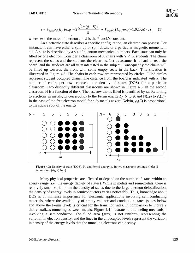
LAB UNIT 5 Scanning Tunneling Microscopy
2009LaboratoryProgram 129
)025.1exp()()(2
2exp)( zEVzEm
EVI FsbiasFsbias ⋅−∝⎥⎥⎦
⎤
⎢⎢⎣
⎡ −−∝ φρ
φρ
�, (1)
where m is the mass of electron and ħ is the Planck’s constant. An electronic state describes a specific configuration, an electron can possess. For
instance, it can have either a spin up or spin down, or a particular magnetic momentum etc. A state is described by a set of quantum mechanical numbers. Each state can only be filled by one electron. Consider a classroom of X chairs with Y < X students. The chairs represent the states and the students the electrons. Let us assume, it is hard to read the board, and the students are all very interested in the subject. Consequently the chairs will be filled up towards the front with some empty seats in the back. This situation is illustrated in Figure 4.3. The chairs in each row are represented by circles. Filled circles represent student occupied chairs. The distance from the board is indicated with x. The number of chairs per row represents the density of states (DOS) for a particular classroom. Two distinctly different classrooms are shown in Figure 4.3. In the second classroom N is a function of the x. The last row that is filled is identified by xF. Returning to electrons in metals; xF corresponds to the Fermi energy Ef, N to ρs and N(xF) to ρs(Ef). In the case of the free electron model for s-/p-metals at zero Kelvin, ρs(E) is proportional to the square root of the energy.
N = 5 5 5 5 5 5 N = 6 6 5 3 3 2 1
Figure 4.3: Density of state (DOS), N, and Fermi energy xF in two classroom settings. (left) N is constant. (right) N(x).
Many physical properties are affected or depend on the number of states within an
energy range (i.e., the energy density of states). While in metals and semi-metals, there is relatively small variation in the density of states due to the large electron delocalization, the density of energy levels in semiconductors varies noticeably. Thus, knowledge about DOS is of immense importance for electronic applications involving semiconducting materials, where the availability of empty valence and conduction states (states below and above the Fermi level) is crucial for the transition rates. In comparison to Figure 2 that visualizes tunneling between metals, Figure 4.4 illustrates the tunneling mechanism involving a semiconductor. The filled area (grey) is not uniform, representing the variation in electron density, and the lines in the unoccupied levels represent the variation in density of the energy levels that the tunneling electrons can occupy.
x xF
x xF
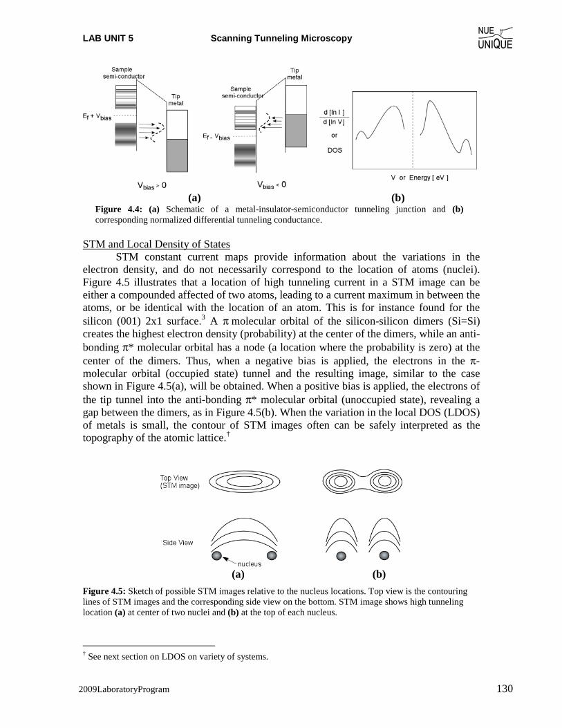
LAB UNIT 5 Scanning Tunneling Microscopy
2009LaboratoryProgram 130
(a) (b) Figure 4.4: (a) Schematic of a metal-insulator-semiconductor tunneling junction and (b) corresponding normalized differential tunneling conductance.
STM and Local Density of States
STM constant current maps provide information about the variations in the electron density, and do not necessarily correspond to the location of atoms (nuclei). Figure 4.5 illustrates that a location of high tunneling current in a STM image can be either a compounded affected of two atoms, leading to a current maximum in between the atoms, or be identical with the location of an atom. This is for instance found for the silicon (001) 2x1 surface.3 A π molecular orbital of the silicon-silicon dimers (Si=Si) creates the highest electron density (probability) at the center of the dimers, while an anti-bonding π* molecular orbital has a node (a location where the probability is zero) at the center of the dimers. Thus, when a negative bias is applied, the electrons in the π-molecular orbital (occupied state) tunnel and the resulting image, similar to the case shown in Figure 4.5(a), will be obtained. When a positive bias is applied, the electrons of the tip tunnel into the anti-bonding π* molecular orbital (unoccupied state), revealing a gap between the dimers, as in Figure 4.5(b). When the variation in the local DOS (LDOS) of metals is small, the contour of STM images often can be safely interpreted as the topography of the atomic lattice.†
(a) (b) Figure 4.5: Sketch of possible STM images relative to the nucleus locations. Top view is the contouring lines of STM images and the corresponding side view on the bottom. STM image shows high tunneling location (a) at center of two nuclei and (b) at the top of each nucleus.
† See next section on LDOS on variety of systems.
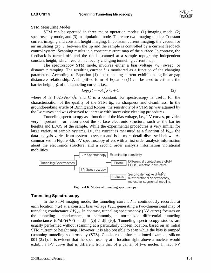
LAB UNIT 5 Scanning Tunneling Microscopy
2009LaboratoryProgram 131
STM Measuring Modes STM can be operated in three major operation modes: (1) imaging mode, (2) spectroscopy mode, and (3) manipulation mode. There are two imaging modes: Constant current imaging and constant height imaging. In constant current imaging, the vacuum or air insulating gap, z, between the tip and the sample is controlled by a current feedback control system. Scanning results in a constant current map of the surface. In contrast, the feedback is turned off, and the tip is scanned at a sample topography independent constant height, which results in a locally changing tunneling current map. The spectroscopy STM mode, involves either a bias voltage Vbias sweep, or distance z ramping. The resulting current I is monitored as a function of the changing parameters. According to Equation (1), the tunneling current exhibits a log-linear gap distance z relationship. A simplified form of Equation (1) can be used to estimate the barrier height, φ, of the tunneling current, i.e., CzAILog +⋅−= φ)( (2)
where A is 1.025 eV /Å, and C is a constant. I-z spectroscopy is useful for the characterization of the quality of the STM tip, its sharpness and cleanliness. In the groundbreaking article of Binnig and Rohrer, the sensitivity of a STM tip was attained by the I-z curves and was observed to increase with successive cleaning procedures.
Tunneling spectroscopy as a function of the bias voltage, i.e., I-V curves, provides very important information about the surface electronic structure, such as the barrier heights and LDOS of the sample. While the experimental procedures is very similar for large variety of sample systems, i.e., the current is measured as a function of Vbias, the data analysis varies from system to system and is in more detail discussed below. As summarized in Figure 4.6, I-V spectroscopy offers with a first order analysis information about the electronics structure, and a second order analysis information vibrational mobilities.
Figure 4.6: Modes of tunneling spectroscopy.
Tunneling Spectroscopy ' In the STM imaging mode, the tunneling current I is continuously recorded at each location (x,y) at a constant bias voltage Vbias, generating a two-dimensional map of tunneling conductance I/Vbias. In contrast, tunneling spectroscopy (I-V curve) focuses on the tunneling conductance, or commonly, a normalized differential tunneling conductance (dI/dV)/(I/V) = d[ln (I)] / d[ln(V)]. Tunneling spectroscopy studies are usually performed without scanning at a particularly chosen location, based on an initial STM current or height map. However, it is also possible to scan while the bias is ramped (scanning tunneling spectroscopy (STS). Consider the aforementioned example, silicon 001 (2x1), it is evident that the spectroscopy at a location right above a nucleus would exhibit a I-V curve that is different from that of a center of two nuclei. In fact I-V
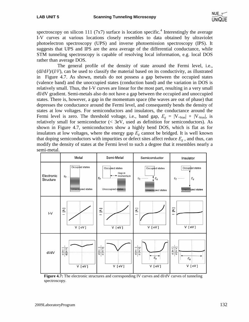
LAB UNIT 5 Scanning Tunneling Microscopy
2009LaboratoryProgram 132
spectroscopy on silicon 111 (7x7) surface is location specific.4 Interestingly the average I-V curves at various locations closely resembles to data obtained by ultraviolet photoelectron spectroscopy (UPS) and inverse photoemission spectroscopy (IPS). It suggests that UPS and IPS are the area average of the differential conductance, while STM tunneling spectroscopy is capable of resolving local information, e.g. local DOS rather than average DOS.
The general profile of the density of state around the Fermi level, i.e., (dI/dV)/(I/V), can be used to classify the material based on its conductivity, as illustrated in Figure 4.7. As shown, metals do not possess a gap between the occupied states (valence band) and the unoccupied states (conduction band) and the variation in DOS is relatively small. Thus, the I-V curves are linear for the most part, resulting in a very small dI/dV gradient. Semi-metals also do not have a gap between the occupied and unoccupied states. There is, however, a gap in the momentum space (the waves are out of phase) that depresses the conductance around the Fermi level, and consequently bends the density of states at low voltages. For semiconductors and insulators, the conductance around the Fermi level is zero. The threshold voltage, i.e., band gap, Eg = |V+bias| + |V-bias|, is relatively small for semiconductor (< 3eV, used as definition for semiconductors). As shown in Figure 4.7, semiconductors show a highly bend DOS, which is flat as for insulators at low voltages, where the energy gap Eg cannot be bridged. It is well known that doping semiconductors with impurities or defect sites affect reduce Eg , and thus, can modify the density of states at the Fermi level to such a degree that it resembles nearly a semi-metal.
Figure 4.7: The electronic structures and corresponding IV curves and dI/dV curves of tunneling spectroscopy.
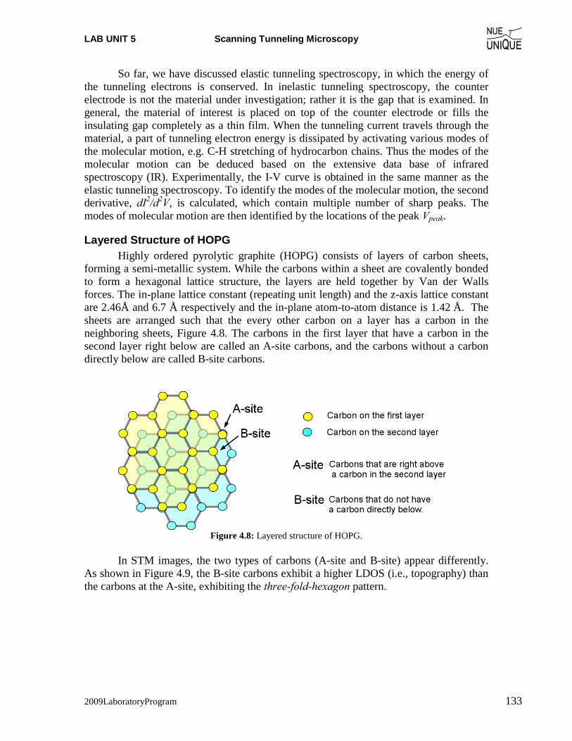
LAB UNIT 5 Scanning Tunneling Microscopy
2009LaboratoryProgram 133
So far, we have discussed elastic tunneling spectroscopy, in which the energy of the tunneling electrons is conserved. In inelastic tunneling spectroscopy, the counter electrode is not the material under investigation; rather it is the gap that is examined. In general, the material of interest is placed on top of the counter electrode or fills the insulating gap completely as a thin film. When the tunneling current travels through the material, a part of tunneling electron energy is dissipated by activating various modes of the molecular motion, e.g. C-H stretching of hydrocarbon chains. Thus the modes of the molecular motion can be deduced based on the extensive data base of infrared spectroscopy (IR). Experimentally, the I-V curve is obtained in the same manner as the elastic tunneling spectroscopy. To identify the modes of the molecular motion, the second derivative, dI2/d2V, is calculated, which contain multiple number of sharp peaks. The modes of molecular motion are then identified by the locations of the peak Vpeak.
Layered Structure of HOPG Highly ordered pyrolytic graphite (HOPG) consists of layers of carbon sheets,
forming a semi-metallic system. While the carbons within a sheet are covalently bonded to form a hexagonal lattice structure, the layers are held together by Van der Walls forces. The in-plane lattice constant (repeating unit length) and the z-axis lattice constant are 2.46Å and 6.7 Å respectively and the in-plane atom-to-atom distance is 1.42 Å. The sheets are arranged such that the every other carbon on a layer has a carbon in the neighboring sheets, Figure 4.8. The carbons in the first layer that have a carbon in the second layer right below are called an A-site carbons, and the carbons without a carbon directly below are called B-site carbons.
Figure 4.8: Layered structure of HOPG.
In STM images, the two types of carbons (A-site and B-site) appear differently. As shown in Figure 4.9, the B-site carbons exhibit a higher LDOS (i.e., topography) than the carbons at the A-site, exhibiting the three-fold-hexagon pattern.
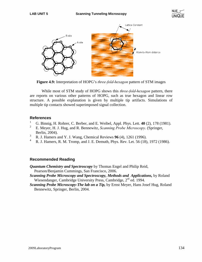
LAB UNIT 5 Scanning Tunneling Microscopy
2009LaboratoryProgram 134
Figure 4.9: Interpretation of HOPG’s three-fold-hexagon pattern of STM images
While most of STM study of HOPG shows this three-fold-hexagon pattern, there are reports on various other patterns of HOPG, such as true hexagon and linear row structure. A possible explanation is given by multiple tip artifacts. Simulations of multiple tip contacts showed superimposed signal collection.
References 1 G. Binnig, H. Rohrer, C. Berber, and E. Weibel, Appl. Phys. Lett. 40 (2), 178 (1981). 2 E. Meyer, H. J. Hug, and R. Bennewitz, Scanning Probe Microscopy. (Springer,
Berlin, 2004). 3 R. J. Hamers and Y. J. Wang, Chemical Reviews 96 (4), 1261 (1996). 4 R. J. Hamers, R. M. Tromp, and J. E. Demuth, Phys. Rev. Let. 56 (18), 1972 (1986).
Recommended Reading
Quantum Chemistry and Spectroscopy by Thomas Engel and Philip Reid, Pearson/Benjamin Cummings, San Francisco, 2006.
Scanning Probe Microscopy and Spectroscopy, Methods and Applications, by Roland Wiesendanger, Cambridge University Press, Cambridge, 2rd ed. 1994.
Scanning Probe Microscopy-The lab on a Tip, by Ernst Meyer, Hans Josef Hug, Roland Bennewitz, Springer, Berlin, 2004.

WORKSHOP Nanoscience on the Tip
2009LaboratoryProgram 135
Addendum: Standard Operating Procedures (SOP)
Table of Contents 1. Easy Scan 2 AFM System Standard Operational Procedure.................. 136
Startup Procedure .................................................................................................... 136 Shutdown Procedure ............................................................................................... 142
2. Easy Scan 2 AFM Reference Sheets......................................................... 143 3. Force Displacement Measurements with Easy Scan 2 ........................... 145 4. Safety: General Rules for Wet-Chemistry ................................................ 146

Standard Operating Procedures
2009LaboratoryProgram 136
1. Easy Scan 2 AFM System Standard Operational Procedure
Startup Procedure
1 Take the Scan Head out from the Scan Head Case and place it on the AFM Sample Stage
Note: Whenever the Scan Head is handled, take the extreme care!
2 Connect Cables a. Connect Scan Head Cable using the screwdriver at the spiral cable connector of
the Scan Head and at the scan head cable connector on the Controller. b. Connect Video Camera Cable at the camera connector of the Scan Head and at
the video in connector on the Controller c. Check if Main Power Cable and USB Cable are connected appropriately.
Easy Scan 2AFM System with optional break-out box

Standard Operating Procedures
2009LaboratoryProgram 137
3 Mount the Cantilever
a. Place the Scan Head up-side-down on a flat space on the AFM work station. b. Slide in the Drop Stop over the detection system as shown below. The Drop Stop
prevents from dropping the cantilever accidentally into the scan head.
Schematic of signal detection system Sliding the
Drop Stop
c. Confirm a blank cantilever (for storage) is placed at the cantilever holder. d. Place the Cantilever Insertion Tool into the hole behind the alignment chip. This
opens the cantilever holder spring. (See below) Note: The Cantilever Holder Spring is very delicate. Do not bend.
e. Use the tweezers to remove the blank cantilever from the holder. i. Hold lightly the cantilever on the sides with the tweezers. ii. Slide it out onto the Drop Stop and rest it. iii. Again hold the cantilever with the tweezers to transfer into a cantilever case.
The Cantilever Insertion Tool opens the cantilever holder spring.
Hold the sides of the cantilever lightly and slide it out onto the Drop Stop
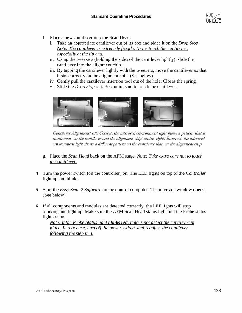
Standard Operating Procedures
2009LaboratoryProgram 138
f. Place a new cantilever into the Scan Head.
i. Take an appropriate cantilever out of its box and place it on the Drop Stop. Note: The cantilever is extremely fragile. Never touch the cantilever, especially at the tip end.
ii. Using the tweezers (holding the sides of the cantilever lightly), slide the cantilever into the alignment chip.
iii. By tapping the cantilever lightly with the tweezers, move the cantilever so that it sits correctly on the alignment chip. (See below)
iv. Gently pull the cantilever insertion tool out of the hole. Closes the spring. v. Slide the Drop Stop out. Be cautious no to touch the cantilever.
g. Place the Scan Head back on the AFM stage. Note: Take extra care not to touch the cantilever.
4 Turn the power switch (on the controller) on. The LED lights on top of the Controller
light up and blink.
5 Start the Easy Scan 2 Software on the control computer. The interface window opens. (See below)
6 If all components and modules are detected correctly, the LEF lights will stop
blinking and light up. Make sure the AFM Scan Head status light and the Probe status light are on.
Note: If the Probe Status light blinks red, it does not detect the cantilever in place. In that case, turn off the power switch, and readjust the cantilever following the step in 3.
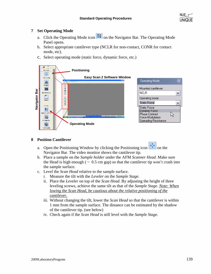
Standard Operating Procedures
2009LaboratoryProgram 139
7 Set Operating Mode a. Click the Operating Mode icon on the Navigator Bar. The Operating Mode
Panel opens. b. Select appropriate cantilever type (NCLR for non-contact, CONR for contact
mode, etc). c. Select operating mode (static force, dynamic force, etc.)
Nav
igat
or B
ar
Positioning
Operating Mode
Easy Scan 2 Software Window
8 Position Cantilever
a. Open the Positioning Window by clicking the Positioning icon on the Navigator Bar. The video monitor shows the cantilever tip.
b. Place a sample on the Sample holder under the AFM Scanner Head. Make sure the Head is high enough ( ~ 0.5 cm gap) so that the cantilever tip won’t crash into the sample surface.
c. Level the Scan Head relative to the sample surface. i. Measure the tilt with the Leveler on the Sample Stage. ii. Place the Leveler on top of the Scan Head. By adjusting the height of three
leveling screws, achieve the same tilt as that of the Sample Stage. Note: When lowing the Scan Head, be cautious about the relative positioning of the cantilever.
iii. Without changing the tilt, lower the Scan Head so that the cantilever is within 1 mm from the sample surface. The distance can be estimated by the shadow of the cantilever tip. (see below)
iv. Check again if the Scan Head is still level with the Sample Stage.
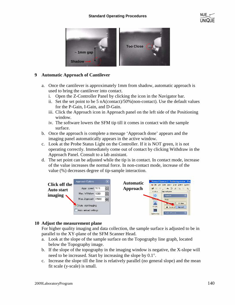
Standard Operating Procedures
2009LaboratoryProgram 140
Shadow
Too Close~ 1mm gap
9 Automatic Approach of Cantilever
a. Once the cantilever is approximately 1mm from shadow, automatic approach is used to bring the cantilever into contact. i. Open the Z-Controller Panel by clicking the icon in the Navigator bar. ii. Set the set point to be 5 nA(contact)/50%(non-contact). Use the default values
for the P-Gain, I-Gain, and D-Gain. iii. Click the Approach icon in Approach panel on the left side of the Positioning
window. iv. The software lowers the SFM tip till it comes in contact with the sample
surface. b. Once the approach is complete a message ‘Approach done’ appears and the
imaging panel automatically appears in the active window. c. Look at the Probe Status Light on the Controller. If it is NOT green, it is not
operating correctly. Immediately come out of contact by clicking Withdraw in the Approach Panel. Consult to a lab assistant.
d. The set point can be adjusted while the tip is in contact. In contact mode, increase of the value increases the normal force. In non-contact mode, increase of the value (%) decreases degree of tip-sample interaction.
10 Adjust the measurement plane For higher quality imaging and data collection, the sample surface is adjusted to be in parallel to the XY-plane of the SFM Scanner Head. a. Look at the slope of the sample surface on the Topography line graph, located
below the Topography image. b. If the slope of the topography in the imaging window is negative, the X-slope will
need to be increased. Start by increasing the slope by 0.1°. c. Increase the slope till the line is relatively parallel (no general slope) and the mean
fit scale (y-scale) is small.
Automatic Approach
Click off the Auto start imaging

Standard Operating Procedures
2009LaboratoryProgram 141
d. If the slope is positive decrease the slope by -0.1.
e. Once the slope is adjusted, the Y-direction slope is also adjusted. To do so, change the scan direction by typing in 90 ° in Rotation in Imaging Area window in the Imaging panel. Adjust the Y-slope in the same manner as X-slope.
11 Adjust the Controller Settings
Click on the Z-controller icon found on the Navigating bar (see below) and adjust the controller settings to keep tip-sample interactions constant. This is done by adjusting the feedback parameters, P, I, and D gain of the Z-controller. i. Leave the P-gain at default value. Increase I-gain by 10% of the default value.
Check in the topographic image if the contrast improves. If it shows a periodic stripe (shown in figure below), the I-gain is generating noise. Reduce it till the noise disappears.
ii. Increase the P-gain by 10 % of that default value. Stop when increasing the P-gain does not improve.
12 Ready for measurements. Proceed with instrument operational instructions specific to the lab unit.
Image Rotation
Noise
Z-Controller Icon
Gain: Proport. Integral
X-Slope Y-Slope
Measured slope

Standard Operating Procedures
2009LaboratoryProgram 142
Shutdown Procedure (1) Retract the cantilever as far as possible by auto-positioning. (2) Close the Easy Scan 2 soft ware window.
(3) Remove the cantilever (follow the instruction given in the Startup procedure step
(3)), and place the blank cantilever for the storage.
(4) Turn of the power switch on the Controller.
(5) Disconnect the Scan Head Cable and the Video Camera Cable.
(6) Place the Scan Head in the Scan Head Case.
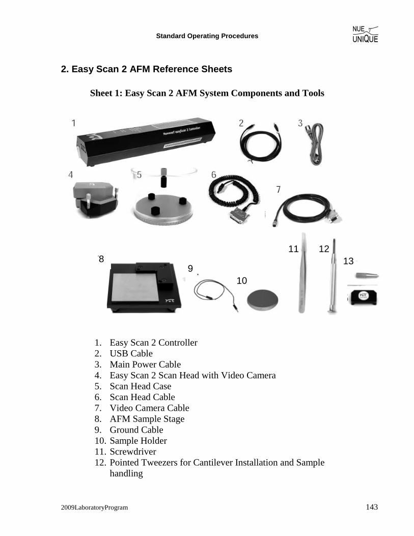
Standard Operating Procedures
2009LaboratoryProgram 143
2. Easy Scan 2 AFM Reference Sheets
Sheet 1: Easy Scan 2 AFM System Components and Tools
1. Easy Scan 2 Controller 2. USB Cable 3. Main Power Cable 4. Easy Scan 2 Scan Head with Video Camera 5. Scan Head Case 6. Scan Head Cable 7. Video Camera Cable 8. AFM Sample Stage 9. Ground Cable 10. Sample Holder 11. Screwdriver 12. Pointed Tweezers for Cantilever Installation and Sample
handling
8 9
10
11 12 13
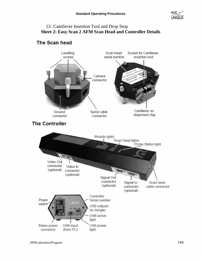
Standard Operating Procedures
2009LaboratoryProgram 144
13. Cantilever Insertion Tool and Drop Stop Sheet 2: Easy Scan 2 AFM Scan Head and Controller Details

Standard Operating Procedures
2009LaboratoryProgram 145
3. Force Displacement Measurements with Easy Scan 2 1. Click ‘Spec’ in the imaging window. The spectroscopy (force-displacement
measurement) window will open. 2. In the Modulation (in Spectroscopy window), set the Start value to 0.5micron and the
End value to 50nm. If high adhesion is expected, change the start value to 1- 3 micron.
3. Click on the topography image once. 4. On the spectroscopy bar, select Point and select a point in the image you would like
to study. 5. Select Start on the spectroscopy bar and a F-D curve will appear in the Deflection-
Spec forward chart. 6. If the entire F-D Curve is not visible in the chart, the chart will have to be scaled by
clicking the ‘scale out’ button. The scale adjust buttons are shown below. 7. Once the entire F-D curve is in the Deflection-Spec forward chart, measure the
distance the cantilever jumps out of contact by selecting the measurement tool and placing it as shown in the diagram below.
8. If the measurement does not produce the F-D curve, check the Probe status light. If it is Red or Yellow, come out of contact once and come in contact again.
Point Start Scale
Adjust Measurement Tool
Scaled F-D curve showing measurement lines
Measured Distance

Standard Operating Procedures
2009LaboratoryProgram 146
Nanotechnology Lab Safety Worksheet
4. Safety: General Rules for Wet-Chemistry
� When conducting wet-chemistry, always wear safety goggles, a lab coat, gloves, and toe-covered shoes.
� Always conduct experimental procedures involving chemicals under the hood.
� Never food or drinks in the lab.
� In case of toxic chemical spills, contact your instructor/lab assistant Instructor_______________ lab assistants ________________________
� If you come in contact with toxic chemicals or the toxic chemicals were spilled on you, immediately flush with plenty of water. Locate closest emergency shower and eye wash in the space provided below.
� Dispose of waste as stated in the experimental procedure or as directed by your instructor.
� Read the labels before opening the containers.
� Reagents are first transferred intro secondary containers for use. All secondary containers should be labeled with the name of the reagent and your name and date transferred.
� Read the instruction carefully. Be 100% sure before combining two chemicals. Careless mistakes can result in serious accidents.
. Care must be exercised in the handling of all chemicals. If any chemical is spilled on the
hands, immediately flush with water. If strong acid or base is spilled on the hands, further treatment may also be necessary. If acid or base is spilled on the clothes, flush with water, if possible, and contact your instructor immediately for advice.
. Because of the presence of toxic chemicals in the lab, never eat or drink in the lab. Also do not put objects (pens, pencils, hands, etc.) in the mouth while in the lab. Such objects may have come into contact with toxic substances which could be accidentally ingested in this manner.