A WINDOWS-based program for static and dynamic analysis of ...
75
A WINDOWS-based program for static and dynamic analysis of 2D frame type structures USER’s MANUAL Kolbein Bell May 2014 1 D 2 fap Frame analysis program - 2D E E Version 3.1
Transcript of A WINDOWS-based program for static and dynamic analysis of ...

A WINDOWS-based program
for static and dynamic analysis of
2D frame type structures
USER’s MANUAL
Kolbein Bell
May 2014
1
D2fap Frame analysis
program - 2D
E E
Version 3.1

Content
Preface 4
To the user of fap2D 5
1 Capabilities 6
2 Platform 8
2.1 Requirements 8
2.2 Recommendations 8
3 The structural model 9
3.1 Members 10
3.2 Joints 11
3.3 Boundary conditions 12
3.4 Eccentricities 13
3.5 Spatial loading 13
3.6 Time dependent loading 15
Earthquake loading 16
3.7 Frequency dependent loading 18
3.8 Periodic, none-harmonic loading 18
3.9 Mass 19
3.10 Damping 19
4 The computational model 20
4.1 Basic philosophy 20
4.2 Reference and identification 21
4.3 Elements 22
4.4 Solution 23
5 Modelling structure and loading 24
5.1 GUI basics 24
Keyboard shortcuts 25
5.2 Modelling the structure 25
5.3 Modelling the loading 27
6 Analysis and results 29
6.1 Linear static analysis 29
Computational aspects 29
Typical results 29
6.2 Influence line analysis and extreme response 32
Computational aspects 33
Typical results 33
Page 2
fap2D
6.3 Real time, linear static analysis 36
6.4 Linearized buckling analysis 38
Computational aspects 38
Typical results 39
6.5 Nonlinear static analysis 40
Computational aspects 41
Typical results 42
6.6 Free, undamped vibration analysis 45
Computational aspects 45
Results 46
6.7 Forced vibration analysis - time domain 47
Computational aspects 49
Typical results 50
6.8 Forced vibration analysis - frequency domain 53
Computational aspects 53
Typical results 56
6.9 Earthquake analysis 59
Time integration 59
Response spectrum analysis 64
6.10 Steel design 67
7 Export and import 71
8 Settings and log file 74
Page 3

Preface
The development of program fap2D started at the Department of structural engineering at NTNU - Norwegian University of Science and Technology - in 2006, as a combined project/master thesis for two students. The project, which is still ongoing has so far included 13 students under my supervision. These are:
2006/2007 - Sverre Eide Holst and Magnus Minsaas,2008/2009 - Dagfinn Dale Kloven and Gunnar Stenrud Nilsen,2009/2010 - Jan Kristian Dolven,2010/2011 - Fredrik Larsen, Brita Årvik and Daniel Aase2012/2013 - Frans Erstad, Kristian Pedersen and Erik Aasmundrud.2013/2014 - Torjus Sandviken and Espen Skogsrud.
The program consists of two distinct parts, a graphical user interface (GUI) and a “computational engine” (Frame2D). While the computational engine (Fortran code) has been my responsibility, the implementation of the major part of the program, the GUI (C# and OpenGL), has been carried out by the students.From the start the emphasis has been on the GUI, and our ambition has been to develop a powerful, but above all easy to use analysis tool, suitable for both education and practical engineering work.I would like to thank all the students who have participated in the project. Your efforts have been impressive, and it has been a pleasure to work with you all.
Trondheim in May 2014Kolbein [email protected]
Page 4

To the user of fap2DFirst of all: read the short chapter 2 about requirements and recommen-dations carefully.
Even if your platform satisfies all requirements and recommendations we cannot exclude the possibility that you may still experience strange and/or unexpected performance. The program uses a third party develop-ment tool (from DevExpress); the interaction between this tool and MS Windows and Open GL seems to produce unexpected “behaviour” in some rare instances. We have been able to circumvent some of these unfortunate malfunctions, but we cannot claim they are all gone. If some-thing like this happens you will most likely be able to continue; it may even work the second time around, but more likely you will have to try an alternative route. It is strongly advised to save a copy of your model often.
The program can handle many types of analyses, from linear statics to earthquake analysis. We have carried out extensive testing, but with so many different possibilities and combinations we cannot claim the pro-gram to be free of bugs.
The Department of Structural Engineering at NTNU is not in a position to provide assistance or support for users of fap2D except when the pro-gram is used in connection with course work or other types of study assignments at our department.
Finally it should be emphasized that the Department of Structural Engi-neering at NTNU accepts no responsibility whatsoever for the use of the program and of results obtained by the program. Hence
all use of program fap2D and of results obtained by fap2D are the user’s own responsibility.
It will be appreciated if obvious analysis errors are reported by e-mail to the following address:
This manual does not describe anything in great detail, nor does it describe all possibilities offered by the program. However, it hopefully provides enough information to enable the user to learn by doing, and to clarify the methods used in the various types of analysis.
Page 5

1 Capabilities
For a qualified user, the short version is that fap2D may be used to determine• static response, due to a variety of loading, according to both linear and nonlin-
ear theory (only geometric nonlinearity is considered),• influence lines for specified response parameters due to a “travelling” load train
on a specified “load path” of a completely linear model, including extreme response due to an arbitrary “train” of concentrated forces,
• real time static response of a linear system due to an arbitrary “load train” travel-ling a “load path” along structural members,
• linearized buckling load(s) and the associated buckling mode shape(s), • free, undamped vibration characteristics (frequencies and mode shapes),• forced dynamic response due to arbitrary but deterministic time dependent load-
ing in the time domain,• forced dynamic response due to deterministic harmonic loading in the frequency
domain,• forced dynamic response due to periodic, but non-harmonic, deterministic loading
in the frequency domain, and• linear earthquake analysis, according to Eurocode 8; both numerical integration
of ground acceleration time series and response spectrum analysis are available,for any valid 2D frame type structure.This version also includes design of steel members according to Eurocode 3.The structure is modelled by straight beam and/or curved arch members (circular or parabolic), both of which can accommodate bending moment, shear and axial force, and/or straight bar, cable (tension only) and strut (compression only) members, all of which can only accommodate axial forces. The members are interconnected at joints. Elastic springs, both boundary springs and coupling springs, as well as eccentricities, in the form of rigid, but weightless “arms” at member ends, may also be included.The spatial loading may be uniform or linearly varying distributed load on beam/arch members, concentrated loads, including moments, at joints, prescribed displacements at joints and initial strain (e.g. temperature). The time variation of spatial loading is defined by several different types of time functions - time here is real time in case of forced dynamic response or fictitious time in case of nonlinear static analysis.Boundary conditions, both “external” and “internal” may be specified at joints, in global reference axes or local axes defined at specific joints. An external boundary condition consists of a suppressed degree of freedom (dof), whereas an internal boundary condition is a displacement release (“hinge”) at a joint.The computational model, which consists of only straight beam and axial elements with constant cross sections, is generated automatically from the structural model. Each beam and arch member is replaced by 50 (default number) straight EULER-BERNOULLI beam elements (no shear deformations) or TIMOSHENKO beam elements (with both
Page 6

fap2D Capabilities
bending and shear deformations). Axial members, that is bar (compression and tension), cable (tension only) and strut (compression only) members are all modelled by one beam element (that can only transmit axial force). The user can easily control the number of elements representing a beam/arch member, locally for individual members or globally for all members in the model.All distributed loading on beam/arch members is lumped into statically equivalent concentrated nodal forces.Computed results are nodal displacements, section forces (M, V and N) for each element, maximum and minimum axial stress at both ends of each element for all types of cross sections and maximum shear stress for most cross sections, as well as residual forces at joints (reaction and “hinge” forces). For some types of analyses, x-y plot of specified response parameters are available, and for buckling and free vibration analyses buck-ling factors, vibration frequencies and corresponding modes are determined.The program consists of two distinct parts, a graphical user interface (GUI) and a “computational engine” (Frame2D).
The GUI is programmed in C# and OpenGL, whereas Frame2D is coded in Fortran, the top level subroutines in Fortran 90 and some lower level (library type) subroutines in Fortran 77.The user is concerned with the structural model only; she/he can also influence the computational model, but only via the structural model. The user cannot access the computational model directly, except for results.UnitsSI units are used consistently throughout the program.
It should be emphasized that the current version is a beta version.
program
fap2D
GUI Frame2D
structural model computational model
Page 7

2 Platform
2.1 Requirements
fap2d is developed and tested on Microsoft’s Windows 7 and Windows 8 platforms; it will also run on Windows Vista, but most likely not on earlier Windows versions.Your PC should have a minimum of 2GB of RAM - preferably more - an i3 processor from Intel (or the equivalent from AMD) or better, and it should have a graphics card that is compatible with Open GL 2.1.
2.2 Recommendations
For the program to function properly, we recommend that the following software should be installed on your PC:
.NET 4.5 and Microsoft Office Access Database Engine.The latter is included in Microsoft Office, but it is also available (free of charge) as a separate installation. Both programs are also available from a separate folder in con-nection with the installation procedure for fap2d.We have experienced Open GL related problems on some installations of fap2d and we therefore recommend that you check if you have the latest driver for your graphics card. Open the Device Manager (via the Start menu) and find the name of the manu-facturer and type of card (under Display Adapters); go to the manufacturer’s web page and follow their instructions for finding the latest driver for your combination of operating system and card type.Even though it makes text and other items quite small, we recommend that you use the smallest DPI setting for your screen, that is the 100% setting; if not, some dialog boxes may be somewhat amputated.
Page 8
3 The structural model
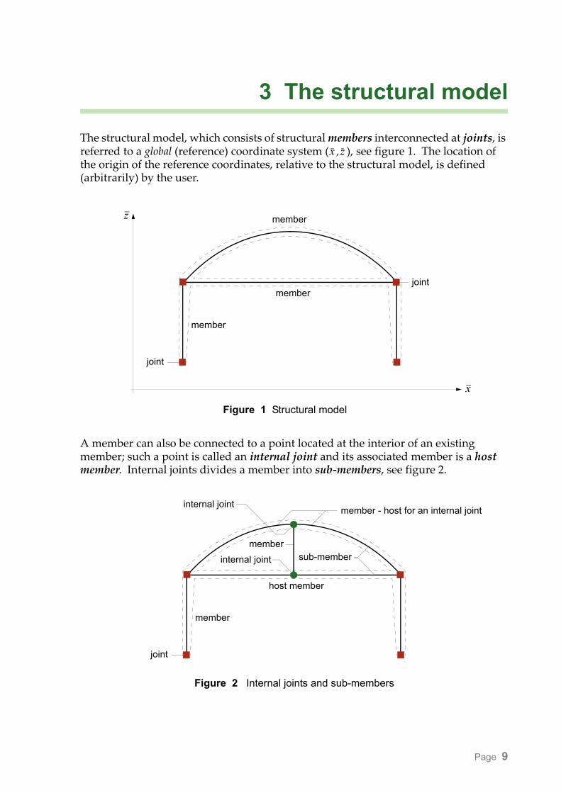
The structural model, which consists of structural members interconnected at joints, is referred to a global (reference) coordinate system ( , ), see figure 1. The location of the origin of the reference coordinates, relative to the structural model, is defined (arbitrarily) by the user.
A member can also be connected to a point located at the interior of an existing member; such a point is called an internal joint and its associated member is a host member. Internal joints divides a member into sub-members, see figure 2.
x z
member
member
member
joint
joint
Figure 1 Structural model
x
z
member
host member
member - host for an internal joint
joint
internal joint
member
internal joint
sub-member
Figure 2 Internal joints and sub-members
Page 9

fap2D The structural model
3.1 Members
The following types of structural members are available:• Straight beam members - henceforth called beam members.• Curved beam members - henceforth called arch members;
arch members may have circular or parabolic shape.• Straight bar members - axial force only - both tension and compression.• Straight cable members - axial tension only (bi-linear elastic behaviour).• Straight strut members - axial compression only (bi-linear elastic behaviour).
In addition to these types of members, elastic springs, both boundary springs (support-ing a particular displacement component) and coupling springs (connecting two similar displacement components or degrees of freedom at coinciding nodes) can also be applied to the structural model.The cross section of a member belongs to one of the following three categories:1. Predefined, that is standardized (steel) sections whose properties are tabulated.2. Parametric, that is a cross section with a geometric form (rectangle, circular tube
etc.) that is uniquely defined by a set of “geometric parameters”, and for which the necessary “mechanical properties” are determined by the program using the geometric parameters.
3. General or arbitrary, that is, a cross section of arbitrary shape and whose section properties (A, I, etc.) are input to the program (obtained for instance by special-ized cross section programs).
For structural members the following rules apply:a) A particular member, regardless of type, has the same material properties
throughout.b) A particular member, regardless of type, has the same cross section shape
throughout, and with one exception the cross section is constant within the member. The exception is beam and arch members having cross sections of the parametric category. In this case, although the shape is the same, the size can vary from one joint to the next. The individual shape parameters (e.g. height, width, radius etc.) of the cross section may vary linearly from one joint to the next.NOTE: An internal joint may define a cross section for its host member, but
only if the cross section is of the parametric category, and of the same shape as that of its host member. Hence, it is possible to describe a completely arbitrary variation of the parametric cross sections along beam and arch members.
c) Straight beam members can be divided into two or more, shorter, but in all other respects ordinary members that will inherit all properties of the mother mem-ber, including its loading. Being “ordinary” members means that they can (after “creation”) be assigned new properties, irrespective of the mother member (they no longer have any recollection of their mother member).NOTE: Arch members can be divided into sub-members, but they cannot be divided
into ordinary members.
Page 10

fap2D The structural model
NOTE: Both beam and arch members can be divided into sub-members by introducing internal joints. However, the sub-member remains an integral part of its host member; the only properties it can have that differ from those of the host member are associated with distributed loading and initial strain (temperature), and, if the host member cross section is of the parametric type, one or more of its parameters can be assigned different values for different sub-members.
Figure 3 shows arch members of circular and parabolic type. Regardless of how they are created, they are uniquely defined by the coordinates of the base points A and B, and the radius of curvature (R) and height (h), respectively. As explained below in the
joint section, arch members are somewhat sensitive to changes made to the position of base points A and B and/or R and h.
3.2 Joints
The following rules apply:1) If a joint is deleted, all members connected to it are automatically deleted.
However, the opposite does not apply: if all members connected to a joint are deleted, the joint is not deleted.It follows from this that joints take precedence over members, i.e. members are connected to joints, not the other way around.
2) An internal joint resides at the interior of a host member. If an internal joint is deleted, all members connected to it, except its host member, are deleted.
3) The position of a joint may be changed arbitrarily. For an arch member con-nected to a joint that is moved, the move will have certain consequences explained below. For all other members the move means change of length and/or orientation.
4) The position of an internal joint may be changed, but only along the host mem-ber axis.
5) Internal joints may be introduced in one of four ways:a) by placing it on the axis of an existing beam or arch member, which then becomes a host member for the internal joint,b) by subdividing an ordinary beam or arch member,c) by joining a new member to a point located at the interior of an existing member; the latter becomes the host member for the internal joint, and finallyd) by applying a concentrated load to a point “inside” a member (concen-trated or point loads can only act at a joint or internal joint).
NOTE: An internal joint can only have one host member.
RA
B
circular arch memberparabolic arch member
A
Bh
Figure 3 Arch members
Page 11

fap2D The structural model
What happens if the shape of an arch is changed, by moving one or both of its base points (A and B) and/or by changing the parameter R or h?If the member has no internal joints, there is no problem. The member’s geometric definition is simply updated. If, however, the member has internal joints, a well defined and unique procedure for the new location of the internal joints is necessary. By definition, they reside on the new position of the member axis, and their relative distance from the first base point (A) is the same as before the change, measured along the chord (which is the straight line between A and B).Both members and joints are numbered, in the order they are created. While internal joints are included in the joint numbering series, the sub-members are not numbered. The numbers may be shown or hidden. Depending on how the model is established, the numbering can be quite erratic and it may thus prove useful to use the renum-bering facility (located in the toolbox).
3.3 Boundary conditions
Boundary conditions are defined at joints. All joints and internal joints will become nodal points in the computational model and as such each has three kinematic degrees of freedom, two orthogonal displacements and one rotation. Any one degree of freedom may be
• free or unknown,• suppressed, which means it has a fixed value of zero,• prescribed, which means it has a fixed, non-zero value, or it may be• dependant of (coupled to) another (free) degree of freedom.
Figure 4 shows the various possibilities of suppressing degrees of freedom at a joint, along with their symbols.
A prescribed dof can only be imposed on a suppressed dof. In other words, a pre-scribed dof, which in most cases will result in an indirect loading effect, is imposed by “moving” a support.A dependant dof is defined by the simple constraint equation:
all 3 dofs are suppressed
the two translational dofs are suppressed
one translational dof is suppressed
one translational and the rotational dof are suppressed
the rotational dof is suppressed
Figure 4 Suppressed degrees of freedom
rs rm=
Page 12
fap2D The structural model
where the dependent or slave dof, rs , is set equal to a master dof, rm , which must be a free dof. This simple slave concept is the tool provided for modelling all types of “hinges” or displacement releases. However, the details of this are all well hidden for the user. The constraint equations required to handle a displacement release are auto-matically created by the program once the user has defined (in a fairly intuitive way) the kind of release he or she wishes to introduce.It should be noted that the degrees of freedom at a joint follow the coordinate axes at the joint. This will be the global axes unless the user has defined local axes at the joint, which she/he can do at any joint or internal joint of the model.Suppressed, prescribed and dependent dofs are collectively referred to as specified dofs. By this terminology we have two types of dofs, free (or unknown) dofs and specified (or known) dofs.Instead of, or in combination with, specified dofs, elastic springs may be used to simu-late boundary constraints. One example of effective combination is the modelling of a semi-rigid joint. A coupling spring may be attached to the degrees of freedom created at a joint through a releasing “hinge”.
3.4 Eccentricities
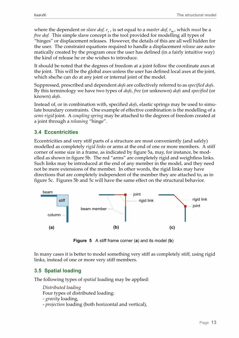
Eccentricities and very stiff parts of a structure are most conveniently (and safely) modelled as completely rigid links or arms at the end of one or more members. A stiff corner of some size in a frame, as indicated by figure 5a, may, for instance, be mod-elled as shown in figure 5b. The red “arms” are completely rigid and weightless links. Such links may be introduced at the end of any member in the model, and they need not be mere extensions of the member. In other words, the rigid links may have directions that are completely independent of the member they are attached to, as in figure 5c. Figures 5b and 5c will have the same effect on the structural behavior.
In many cases it is better to model something very stiff as completely stiff, using rigid links, instead of one or more very stiff members.
3.5 Spatial loading
The following types of spatial loading may be applied:Distributed loadingFour types of distributed loading:- gravity loading,- projection loading (both horizontal and vertical),
stiff
beam member
rigid link
jointbeam
column
Figure 5 A stiff frame corner (a) and its model (b)
(a) (b)
rigid link
joint
(c)
Page 13
fap2D The structural model
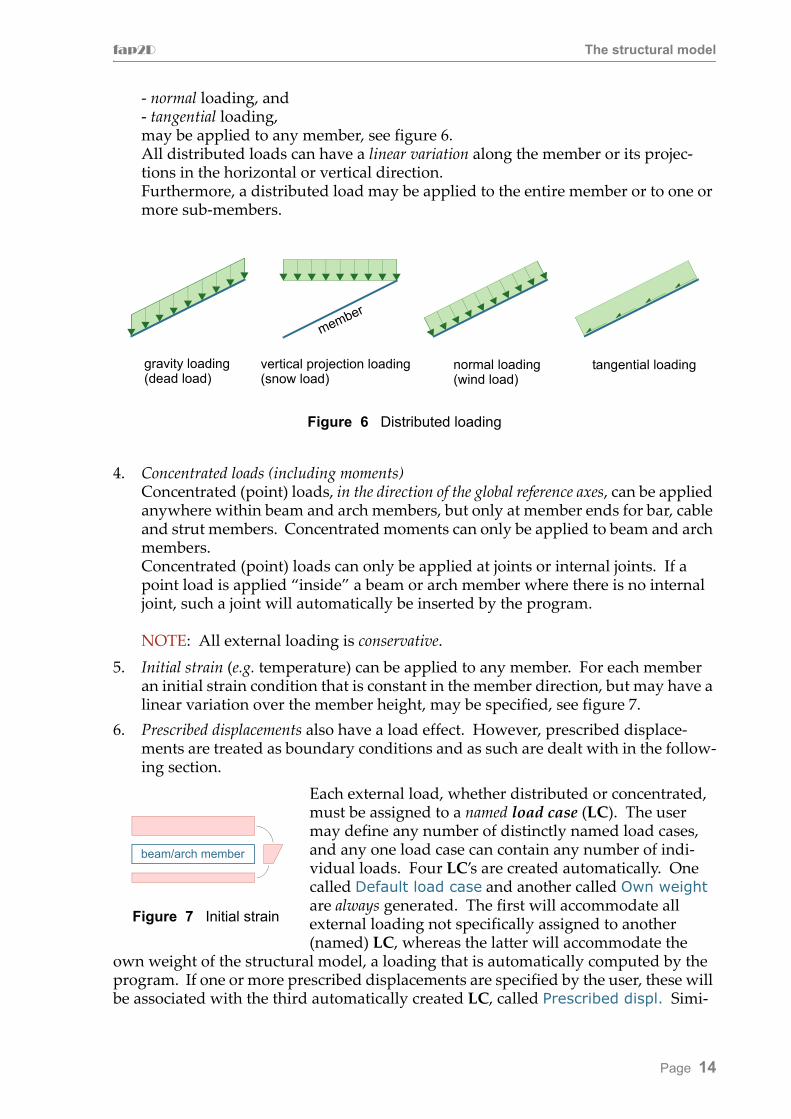
- normal loading, and- tangential loading,may be applied to any member, see figure 6. All distributed loads can have a linear variation along the member or its projec-tions in the horizontal or vertical direction.Furthermore, a distributed load may be applied to the entire member or to one or more sub-members.
4. Concentrated loads (including moments)Concentrated (point) loads, in the direction of the global reference axes, can be applied anywhere within beam and arch members, but only at member ends for bar, cable and strut members. Concentrated moments can only be applied to beam and arch members.Concentrated (point) loads can only be applied at joints or internal joints. If a point load is applied “inside” a beam or arch member where there is no internal joint, such a joint will automatically be inserted by the program.
NOTE: All external loading is conservative.5. Initial strain (e.g. temperature) can be applied to any member. For each member
an initial strain condition that is constant in the member direction, but may have a linear variation over the member height, may be specified, see figure 7.
6. Prescribed displacements also have a load effect. However, prescribed displace-ments are treated as boundary conditions and as such are dealt with in the follow-ing section.
Each external load, whether distributed or concentrated, must be assigned to a named load case (LC). The user may define any number of distinctly named load cases, and any one load case can contain any number of indi-vidual loads. Four LC’s are created automatically. One called Default load case and another called Own weight are always generated. The first will accommodate all external loading not specifically assigned to another (named) LC, whereas the latter will accommodate the
own weight of the structural model, a loading that is automatically computed by the program. If one or more prescribed displacements are specified by the user, these will be associated with the third automatically created LC, called Prescribed displ. Simi-
vertical projection loading(snow load)
gravity loading(dead load)
normal loading(wind load)
tangential loading
member
Figure 6 Distributed loading
beam/arch member
Figure 7 Initial strain
Page 14

fap2D The structural model
larly, if temperature and/or any other form of initial strain is defined, all such loading is accommodated by the fourth automatically created load case called Init. strain. It should be noted that a specific model can only have one LC for prescribed displace-ments (Prescribed displ.) and one LC for initial strain/temperature (Init. strain).Computations are carried out for named load combinations (LCmb), not load cases. A spatial load combination is a linear combination of any number of named LC’s. Each selected LC contributes by a user specified constant load factor (the program offers a default load factor of 1,0 which the user of course can change).The user may define any number of distinctly named load combinations, and any one load combination can contain any number of individual LC’s. The program creates automatically one LCmb called Default load combination, which, on creation, con-tains only the Default load case with a load factor of 1,0. If no loads have been assigned to the Default load case, the Default load combination contains no loading. The user may edit the Default load combination by including the Own weight load case and thus obtain results (for own weight only) without having defined any exter-nal loading. It should be noted that Own weight is not automatically included in any LCmb. NOTE: If prescribed displacements have been specified (for suppressed dofs) the Prescribed displ. LC has been created. An analysis carried out for a load combination that do not include this LC, will assume that the dof(s) in question is (are) suppressed.
3.6 Time dependent loading
Time, defined by the time parameter λ, means real time (in seconds) if we are talking about a dynamic analysis, whereas it is fictitious time in the case of a nonlinear static analysis (used to define the loading and response history).Time dependent loading consists of a spatial load combination multiplied by a time-dependent load factor ψ which is referred to as a time function. The program recog-nizes 5 different time function types, valid between 0 and λmax :
Type 1: (constant)
Type 2: (linear between 0 and 1)
Type 3: Arbitrary, but possibly semi-periodic:
ψ3 is defined by np pairs (λi , ψ3i) of numbers and the number (nper) of periods, all of which are input information. The λ-values are measured in terms of time units.The function value varies linearly between the points and the requirements are:
ψ1 1,0=
ψ2λ
λmax-----------=
λp λp λp
1
2
34
5
6
78
ψ3 number of periods (nper) is 3 here
λ
nper
Page 15
fap2D The structural model
λi+1 > λi and (λp × nper) ≤ λmax
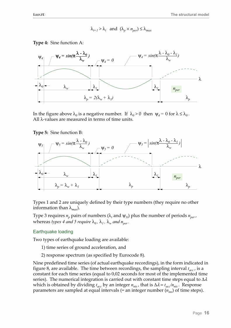
Type 4: Sine function A:
In the figure above λ0 is a negative number. If λ0 > 0 then ψ4 = 0 for λ ≤ λ0 .All λ-values are measured in terms of time units.
Type 5: Sine function B:
Types 1 and 2 are uniquely defined by their type numbers (they require no other information than λmax).Type 3 requires np pairs of numbers (λi and ψ3i) plus the number of periods nper , whereas types 4 and 5 require λ0 , λ1 , λw and nper .
Earthquake loading
Two types of earthquake loading are available:1) time series of ground acceleration, and2) response spectrum (as specified by Eurocode 8).
Nine predefined time series (of actual earthquake recordings), in the form indicated in figure 8, are available. The time between recordings, the sampling interval tacc , is a constant for each time series (equal to 0,02 seconds for most of the implemented time series). The numerical integration is carried out with constant time steps equal to Δλ which is obtained by dividing tacc by an integer nnts , that is Δλ = tacc/nnts . Response parameters are sampled at equal intervals (= an integer number (nins) of time steps).
λw
λp = 2(λw + λ1)
ψ4
λλ0 λ1 λ1
λp
ψ4 = sin(π )λ - λ0
λw ψ4 = 0ψ4 = sin(π )λ - λ0
λw
ψ4 = sin(π )λ - λ0 - λ1
λw
nper
nperλw
λp = λw + λ1
ψ5
λλ0 λ1 λ1
λp
ψ5 = sin(π )λ - λ0
λw ψ5 = 0ψ5 = sin(π )λ - λ0 - λ1
λw
λp
Page 16

fap2D The structural model
Response spectra, in the shape shown in figure 9, are available for earthquake response spectrum analysis. The spectrum is defined by the three time parameters, TB, TC and TD as well as the damping correction factor η and the scale factor S. The damping correction factor η is defined as
where ζ is the damping ratio,
ground acceleration
time
an entry in the time series
tacc
Δλ = tacc/nntssampling point forresponse parameters
Δλ×nins
Figure 8 Time series of earthquake ground accelerations
t (λ)
η 105 100ζ+--------------------- 0,55≥=
TB TC TD T
Se(T )×S
2,5η
0
1,0
2,0
Figure 9 Typical earthquake response spectrum (Eurocode 8)
5% damping (η = 1,0)
Scale factor S = 1,0
Page 17

fap2D The structural model
3.7 Frequency dependent loading
Frequency dependent loading is harmonic, with a variation along the time axis as shown in figure 10. The load frequency is Ω (rad/s) or f (Hz). Program fap2D expects frequencies to be given in Hz, and it recognizes two types of harmonic loading:1. Only one load frequency ( f ). In other words, all loading is harmonic in time and
have the same frequency. However, more than one spatial load combination may be applied, and these may have different phase angles (α). In fact, if the phase angles are not different, it makes little sense to apply more than one spatial load combination, and all spatial loading may as well be lumped into one load combi-nation.
2. Only one spatial load combination is applied as a harmonic load, but it may be applied with many different frequencies, from f1 to fmax , in equal steps of Δf. In this case phase angle has no meaning for the loading.
3.8 Periodic, but non-harmonic loading
This loading is characterized by one or more spatial load combinations and one time function ψ, which is the same for all contributing loading (which can be due to external loading and prescribed displacements). The time function must be of type 3, 4 or 5, see section 3.6.The periodic loading, exemplified in figure 11, is automatically replaced by a series of harmonic load combinations through a Fourier series analysis. The number of Fourier terms included is determined by a user defined tolerance parameter, subject to a
period = T = =2πΩ
1f
R(t)
t
α = 0 α = π2 α = π
2
2πΩf = is the frequency in Hz
Figure 10 Harmonic loading
phase angle
time function (of type 3, 4 or 5)
ψ (load multiplier)
Δλ
period T (= λp )t (λ)
T T
Figure 11 Periodic loading
Page 18

fap2D The structural model
“ceiling” defined by the maximum permissible number of terms, which is also specified by the user.
3.9 Mass
The mass of the structural members may be (automatically) accounted for by one of three mass representation models:
• lumped mass representation - the mass of each element is lumped into two equal concentrated “translational masses” at the element nodes; all rotational dofs are mass-less (this is the program’s default setting),
• consistent mass representation - the element mass matrix is established on the basis of the same displacement functions as the stiffness is derived from; this leads to rotational as well as translational mass, and mass coupling,
• diagonalized mass representation - this is a combination of the other two models; it leads to a diagonal element mass matrix, i.e. both translational and rotational mass, but no mass coupling.NOTE: The theoretical basis for this model is not very well founded.
The basic modelling philosophy adopted by the program (see next chapter) favours the lumped mass approach, and only numerical reasons seem to warrant one of the other two methods. In some (rare) circumstances the lumped approach may lead to numerical difficulties (in the solution of the free vibration eigenproblem).In addition to the mass of the structural members, concentrated (translational and rotational) mass may be introduced at joints, including internal joints.
3.10 Damping
Dynamic analysis may be carried out on the complete (coupled MDOF) model or on a reduced (decoupled SDOF) model obtained through use of a limited number of modal coordinates. Regardless of model, viscous damping is assumed.For the complete MDOF model the available damping model is the so-called Rayleigh damping in which the damping matrix C is expressed as a combination of the mass matrix (M) and the stiffness matrix (K) of the model, that is
The coefficients a1 and a2 may be given explicitly (as input) or they may be computed by the program on the basis of generalized mass and stiffness; more about this later. The user can specify mass proportional damping (a2 = 0), stiffness proportional damping (a1 = 0) or a complete Rayleigh damping (both a1 and a2 have non-zero values).For a complete MDOF model it is also possible to include “point dampers” (viscous dashpots), at any (free, non-specified) dof of any joint, in addition to or instead of the Rayleigh damping.For an SDOF model (that is modal analysis), damping ratios may be specified expli-citly (as input) for each contributing mode, or alternatively the damping ratios may be computed implicitly for each mode using a Rayleigh type approach; more about this later. For this (SDOF model), point dampers cannot be included.
C a1M a2K+=
Page 19

4 The computational model
4.1 Basic philosophy
Once the structural model and its spatial loading is complete one of several analyses may be specified. Depending on the type of analysis some more information may be needed (mostly concerning the loading) before the analysis can be started; more about this later. As and when an analysis starts the structural model is automatically con-verted into a computational model. This transformation is based on the philosophy indicated by figure 12. Beam and arch members are subdivided into a fairly large
number of straight beam elements, each with 6 degrees of freedom and constant cross section properties (determined as the properties at the element’s mid-point). Distri-buted loading, if present, is lumped into statically equivalent concentrated loads at the nodes.For the structural member in figure 12, the number of elements required is probably dictated by the member geometry. However, the idea of load lumping also requires a straight beam member to be subdivided into a series of shorter elements if it is sub-jected to any form of distributed loading (even if the geometry does not call for such subdivision). For a straight member the number of computational elements is dictated by the load representation and possibly also by a varying cross section (which is approximated by step-wise constant section properties).
element (straight and with
Figure 12 Basic modelling concept
load lumping
structural member
load
constant properties)
nodal point (node)
Page 20
fap2D The computational model
This simple strategy leads to a much higher number of degrees of freedom, and thus more numerical work and higher storage demands, than the more conventional approach of one to one relation between member and element. The simplicity of the “brute force” technique, combined with some obvious advantages in describing curved members and geometric imperfections, is believed to more than compensate for the increased computational effort and storage requirements. It also lends itself extremely well for geometric presentation of both model and results - everything boils down to simple straight lines.
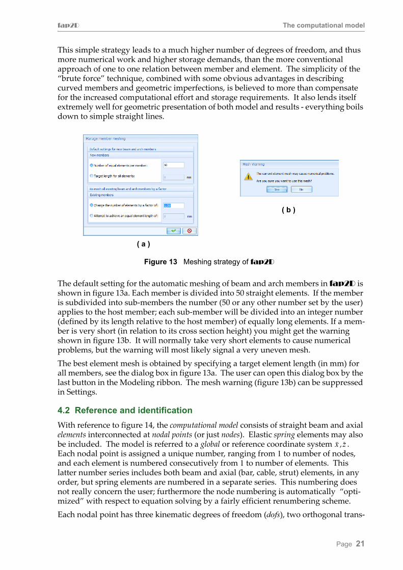
The default setting for the automatic meshing of beam and arch members in fap2D is shown in figure 13a. Each member is divided into 50 straight elements. If the member is subdivided into sub-members the number (50 or any other number set by the user) applies to the host member; each sub-member will be divided into an integer number (defined by its length relative to the host member) of equally long elements. If a mem-ber is very short (in relation to its cross section height) you might get the warning shown in figure 13b. It will normally take very short elements to cause numerical problems, but the warning will most likely signal a very uneven mesh.The best element mesh is obtained by specifying a target element length (in mm) for all members, see the dialog box in figure 13a. The user can open this dialog box by the last button in the Modeling ribbon. The mesh warning (figure 13b) can be suppressed in Settings.
4.2 Reference and identification
With reference to figure 14, the computational model consists of straight beam and axial elements interconnected at nodal points (or just nodes). Elastic spring elements may also be included. The model is referred to a global or reference coordinate system , . Each nodal point is assigned a unique number, ranging from 1 to number of nodes, and each element is numbered consecutively from 1 to number of elements. This latter number series includes both beam and axial (bar, cable, strut) elements, in any order, but spring elements are numbered in a separate series. This numbering does not really concern the user; furthermore the node numbering is automatically “opti-mized” with respect to equation solving by a fairly efficient renumbering scheme.Each nodal point has three kinematic degrees of freedom (dofs), two orthogonal trans-
Figure 13 Meshing strategy of fap2D
( a )
( b )
x z
Page 21

fap2D The computational model
lations and one rotation. By default the dofs, also denoted nodal displacements, are referred to (are parallel with) the global reference axes, and . It is, however, pos-sible to define a local coordinate system, xL , zL , at any node. At such a node the trans-lational dofs follow the local axes.At a node where only axial elements meet, e.g. node 6 in figure 14, the program auto-matically suppresses the rotational dof (which does not receive stiffness contributions from any of the axial elements).
4.3 Elements
The following elements are available:
Beam element - a simple, straight 6-degree-of-freedom element with constant cross section. Bending, axial and shear deformations are considered. The latter, which is based on the assumption of an average shear deformation (Timoshenko theory), is optional.Material properties are linearly elastic, for all types of analysis.Axial element - a simple, straight 4-degree-of-freedom element with constant cross section that can only take axial force. Bi-linear stiffness characteristics may be speci-fied. In other words, a particular axial element may take both tension and compres-sion, in which case it is a bar element, tension only, in which case it is a cable element, or compression only, in which case it is a strut element.
1
2
3
4
5
k
1
2
1
2
3
4
57 8 i
beam element
axial element
nodal point
Figure 14 Typical computational model
nodal degrees of freedom :
xL
zL6
x
z
x z
beam element
- bar element- cable element- strut element
axial element
spring elements(Euler-Bernoulli or Timoshenko)
Page 22

fap2D The computational model
Spring elements - both linear and rotational springs may be included in the model. A spring may be a- boundary spring which is a spring connected to a single degree of freedom at one end and fixed (“to earth”) at the other, or a- coupling spring which is a spring connecting the same type of dof at two nodal points, e.g. the rotation at two nodes - it should be noted that the two nodes normally coincide (geometrically). For most types of analyses the springs are linear, but nonlinear springs are also avail-able (for nonlinear static analysis), see figure 15. In all cases the springs have identical characteristics in tension and compression.
4.4 Solution
The system matrices, stiffness (K), mass (M) and load (R), are assembled to include only the unknown degrees of freedom; in other words, all specified dofs are omitted from the matrices. Stiffness matrices and consistent mass matrices are stored in so-called skyline storage format, and the basic numerical operation of solving a system of linear algebraic equations is accomplished by direct GAUSSIAN elimination, through factorization (LDLT) and substitutions.For the eigenvalue problems (free vibration, modal analysis and linearized buckling) the user can choose between subspace iteration (which is the default method) and a truncated algorithm due to LANCZOS. The latter is by far the most efficient with regard to computational effort; however, subspace iteration is a well tested and fairly robust algorithm.More computational details are given below for the individual types of analysis.
v1
S1 S2
S3S4
S5
v2 v3 v4 v5
S
v
v1 < v2 < v3 < v4 < v5
S1 < S2 < S3 < S4 < S5
Requirement:
up to 5 points may be specified
Figure 15 Nonlinear spring stiffness
stiffness = Si+1 - Sivi+1 - vi
(force or moment)
(displacement or rotation)
Page 23

5 Modelling structure and loading
5.1 GUI basics
Figure 16 shows an overview of the GUI. The panels shown in the figure are also referred to as “dock panels” since they may be docked anywhere in the GUI view.
Figure 17a shows the welcome screen that appears in the modelling panel whenever you open the program. The same functions (plus some more) are also available from
Application menu
Ribbon
Modeling panelToolbox panel
Left panel
Ribbon page
Bottom panel
User ManualMenu line
Figure 16 GUI overview
Pointer coordinates
Figure 17 Welcome screen (a) and application menu (b)
( b )( a )
Page 24

fap2D Modelling structure and loading
the application menu, shown in figure 17b, which is launched by clicking the appli-cation menu button at the top left-hand corner of the display.The program makes use of the ribbon concept, and basically, the user works from left to right. Apart from this manual, a pdf-version of which is available from the ques-tion mark button at the right-hand top corner, there is not much in terms of “help” available. The main design criterion has been to make the use of the program as intui-tive as possible through familiar icons and well designed dialog boxes. Tooltips are available for most buttons.On the whole the left-hand mouse button is the “operation” button (apology to all left-handers!) and the right-hand button is the “information” button.The menu line has four main choices, Modelling, Loading, Analysis and Results. In figure 16 Results is not present since no analysis has, as yet, been exe-cuted. The fifth choice (Appearance) has to do with the style and coloring of the views.
Keyboard shortcuts:
5.2 Modelling the structure
Press Function
CTRL+T & CTRL+N Make a new model
CTRL+S Save the current model
CTRL+O Open an existing model
CTRL+P Print a picture of the current model
CTRL+D & Del Delete marked objects in the model
CTRL+Z Undo
CTRL+Y Redo
CTRL+F4 Close the model
CTRL+TAB Toggle between open models
CTRL+A Mark all objects in the model
ESC Close a dialog box / Reset mouse pointer
ENTER Push the OK-button in dialog boxes
F1 Launch User’s Manual
Figure 18 The modelling ribbon
Page 25

fap2D Modelling structure and loading
How to establish a viable structural model is fairly straightforward; again the “natural” mode of operation is from left to right, see the modelling ribbon in figure 18. The program has predefined 4 materials: Steel, Concrete, Timber and Aluminum, all with typical parameters, which cannot be changed. However, the user may define hers or his own material types by selecting Add/edit in the pull-down menu. Next, all cross sections to be used in the model should be selected (if of predefined category) or defined (if of parametric or arbitrary category); one cross section, an IPE 200, has been preselected and is always available and ready for use.To draw the model we could start by placing the joints explicitly, via the Add joint button, and then draw members between the joints. However, a more efficient way is to start drawing members right away. Select material, cross section and member type and click Draw member. Point to where the member is to start, push the left mouse button and keep it down while you pull the pointer to the end point of the member (creating the member in the process). Release the mouse button and the member with its two end joints have been created. The member properties (material, cross section, type) remain “in the pointer” and you can continue to draw as may members of this type as you wish, either between two new joints or by starting or ending at an existing joint. If you start or end at a point located at the interior of a member, an internal joint will be created, subdividing the member into sub-members, and the new member is attached to the existing one. All beam and arch members are initially rigidly connected at the joints.It should be kept in mind that the program default is to snap a joint to the closest grid point (does not apply to internal joints). Grid spacing and snap can be controlled from the toolbox, but it is also quite straightforward to change the coordinates of a joint once it has been created. It should also be noted that once a specific function has been chosen (for instance by pushing a button), this function remains active (“in the pointer”) until a new function or the neutral pointer is chosen. Figure 19 shows the structural model of a simple frame. The “hinge” at point D, introduced by clicking
the Hinge button and then the joint and follow “instructions” in the emerging dialog box, “decouples” the rotation of the column from that of the beam which is continu-ous over the column.
local axes
rigid “arms”
Figure 19 Structural model of a simple frame
D
A
EC
B
SHS 100×100×10
RHS 200×100×10
grid spacing = 0,5 m
Page 26

fap2D Modelling structure and loading
The function provided by the X-dof button is similar to that of the Hinge button, but it releases displacements instead of rotations. Consider for instance an internal joint of a straight member at which you want to disconnect the displacement along the mem-ber axis. Make sure that the x-axis is parallel with the member axis (transform to local coordinates if necessary), and click the X-dof button function on to the joint. If more than the two sub-members meet at the joint you may need to reconnect some continu-ities; follow instructions in the dialog box (in the same way as for the Hinge button function). This X-dof release will prevent transmission of axial force through the joint. If the x-axis (global or local) at the joint is normal to the sub-members, the imposed release will prevent transmission of shear force.Semi-rigid joints may be simulated by inserting a Coupling spring between “released” member ends (across the imposed discontinuity).In order to include local coordinate axes (point E in figure 19), eccentricities (rigid links at point C) or response parameters, right-click the joint and select the appropriate function from the popup menu which in turn will lead you to a fairly self-explanatory dialog box.
5.3 Modelling the loading
Also the loading ribbon, shown in figure 20, is fairly self explanatory; spatial loading, in terms of load cases (LC), and time functions are defined here. It should be noted that prescribed displacements and initial strain both give rise to spatial loading. All spa-tial loading must be assigned to a particular (named) LC. Two predefined load cases exist, Default load case and Own weight, and the user may define any number of named load cases via the Add/edit command in the drop down menu. Own weight contains the dead load of the structural members themselves, and this loading is auto-matically computed by the program; other loading cannot be assigned to this LC. The Default load case and any user defined LC can accommodate any number of concen-trated loads/moments and/or distributed member loads.If prescribed displacements are defined (at one or more supported joints) the program automatically creates an LC named Prescribed displ.; all prescribed displacements of a particular structural model will be associated with this LC which can only hold prescribed displacements (no other loading). Similarly, if temperature or other types of initial strain are defined for one or more members, the program automatically creates an LC named Init. strain; all loading of type initial strain will be associated with this LC which cannot hold any other type of loading.Named time functions of types 3, 4 or 5 (see the section on time dependent loading on pages 14 and 15) are defined via the Edit time functions button.
Figure 20 The loading ribbon
Page 27
fap2D Modelling structure and loading
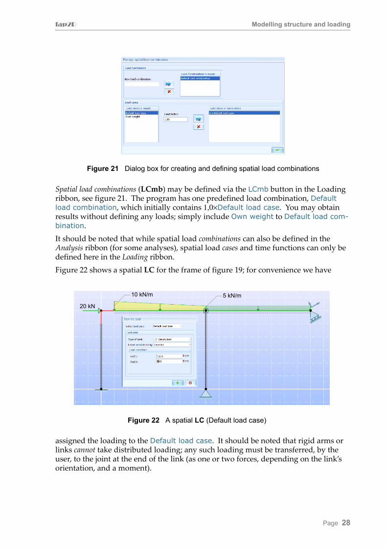
Spatial load combinations (LCmb) may be defined via the LCmb button in the Loading ribbon, see figure 21. The program has one predefined load combination, Default load combination, which initially contains 1,0×Default load case. You may obtain results without defining any loads; simply include Own weight to Default load com-bination.It should be noted that while spatial load combinations can also be defined in the Analysis ribbon (for some analyses), spatial load cases and time functions can only be defined here in the Loading ribbon.Figure 22 shows a spatial LC for the frame of figure 19; for convenience we have
assigned the loading to the Default load case. It should be noted that rigid arms or links cannot take distributed loading; any such loading must be transferred, by the user, to the joint at the end of the link (as one or two forces, depending on the link’s orientation, and a moment).
Figure 21 Dialog box for creating and defining spatial load combinations
Figure 22 A spatial LC (Default load case)
20 kN
10 kN/m 5 kN/m
Page 28

6 Analysis and results
6.1 Linear static analysis
Figure 23 shows the ribbon for linear static analysis. The Run analysis arrow is active, and if pressed the analysis will be carried out without shear deformations for the Default load combination. Shear deformations are either neglected (which is default) or included by pressing the Include shear deformation button; this button toggles off/on. The LCmb drop down menu enables the user to select any existing load com-bination for the analysis; in fact the user can also define new load combinations or edit existing ones from this position (the last item in the drop down menu is Add/edit), but only using existing load cases (LC). If new LCs are required it is necessary to go back to the Loading ribbon.
Computational aspects
The computations are straightforward, and the analysis is carried out for one load combination at a time. By default, shear deformations are not included, but as already mentioned above they are easily included by simply pushing the Include shear deformation button before the Run Analysis button. If bi-linear axial members, that is cable and/or strut members, are present, the model is not strictly linear. In this case the program will make sure, through an iteration procedure, that all cable and strut members carry tension or compression, respectively. During the iteration procedure such members may thus be “removed” from or inserted back into the model, and the iteration continues until no bi-linear members needs to be removed/inserted from one iteration to the next.
Typical results
The frame of figure 19 subjected to the loading shown in figure 22 is analyzed. Suc-cessful completion of the analysis will take the user directly to the result view, see fig-ure 24. The results available are shown in the ribbon. The first of these shows an overview where all four diagrams are shown along with their maximum response as shown in figure 24; this is always the results that appear after a successful analysis. Each of the four diagrams in this view can be selected individually and inspected in more detail. Figure 25 shows the bending moment diagram. It should be noted that this diagram is always drawn on the “tensile side” of the member. The only result accompanying the diagram is the maximum moment value (27,78 kNm not shown in figure 25). However, by right clicking an element, results at the ends of that element are shown in a result box as shown in figure 25. Clicking the σ/τ button in this box
Figure 23 Analysis ribbon for linear static analysis
Page 29

fap2D Analysis and results
will, as shown, produce another box with the axial stress (σx) at the extreme cross sec-tion fibers as well as the maximum shear stress (τ). The latter is not available for cross sections of the arbitrary category. Note also that in the dialog box that appears when you right-click an element, you can step one element at a time, in both directions (using the arrows at the top of the dialog box), or you can go directly to the first or the last element of the member.
Figure 24 Results available for a linear static analysis
Figure 25 Bending moment diagram and detail results
Page 30

fap2D Analysis and results
It should also be noted that the toolbox to the right have changed significantly from the model and load view. All individual diagrams can be scaled up or down by using the arrow buttons in the toolbox or by giving the exact scale factor; they can be nor-malized again using the N button. For the displacement diagram the toolbox provides a button (Tδ) that will show the displacements with “true” (real) size. In all diagrams the point of maximum response is indicated (by a colored circle); this circle can be made to disappear or come back again by the toggle button in the toolbox.Clicking the button Reaction forces (see figure 24) will produce a view of the model with arrows indicating all non-zero reactions; right-clicking the joint symbol will produce a box with the values of the reaction forces. Right-clicking any joint will pro-duce the residual forces at the joint; for an unsupported joint with no displacement releases (”hinge”) these forces should be zero. At a hinge the residual forces are the “hinge forces”, the sum of which should be zero for all members at the joint.The Show resultants button will produce the sum of all external loading in the two global directions as well as the sum of all reaction forces in the same directions.
Page 31

fap2D Analysis and results
6.2 Influence lines and extreme response
Figure 26 shows the ribbon for analysis of influence lines. The Run analysis arrow is
active, but in order to carry out an analysis the user needs to define a load path and one or more response parameters must have been or be defined. Since influence lines are normally used to determine the maximum response to loading “moving” across the load path, such loading, here called a load train, should also be defined prior to the actual analysis.It should be noted that the concepts of load path and load train are also used in con-nection with Real time analysis, but they are not the same; hence the A and B versions.Figure 27 shows the dialog boxes launched by the Define load path and the Define load train buttons, respectively. The load path consists of the members on which the
load train can travel. Figure 27a suggests that the load path can be defined by mark-ing the relevant members before clicking the Define load path button and then click the Add selected members to the load path button (that will be active if this approach is used, as is the case for the dialog box in figure 27a), or the Define load path button can be clicked without any members marked and then exit the box with enable and click the relevant members. The dialog box in figure 27a also lets the user define the size and direction of the moving point load that “produce” the influence line(s) - default is −1,0 kN in the z-direction.A named load train can consist of any number of point loads at arbitrary, but user defined mutual distances (defined by each load’s distance from the first load), and any
Figure 26 Analysis ribbon for analysis of influence lines
Figure 27 Definition of load path (a) and load trains (b)
( a ) ( b )
Page 32
fap2D Analysis and results
number of load trains can be defined. It should be noted that the loads constituting the load train acts in the same direction as the moving point load. Figure 27b shows a load train, named T1, that consists of three point loads, the first of which has a magni-tude of 20 kN whilst the other two both are 30 kN (all acting downwards, in negative z-direction). The distance between the first and the second is 2m whereas the last load follows 3m behind the second one.
Computational aspects
Influence line analysis requires a completely linear model. Hence bi-linear members (cables and/or struts) cannot be present in the structural model (if present they must be removed or converted into bar members before an analysis is attempted). The computations consist of a (large) series of linear static analyses, one for each load situ-ation. A load situation in turn consists of the moving point load placed at a nodal point of a member of the load path. The number of load situations, i.e. the number of load vectors, is therefore defined by the total number of nodal points in the load path members.Since the model is linear, the stiffness matrix is formed and factorized once, and for each load situation the solution is obtained by forward and backward substitutions (which are “cheap” operations compared with factorization). For each load situation the response parameters are computed and stored for presentation. For a particular response parameter each such computed value is drawn as a scaled line segment perpendicular to the horizontal (vertical) projection of the travel path, starting from the x- (z-) coordinate of the node in question. The influence line of this particular response parameter is the line drawn through the end points of these scaled lines.
Typical results
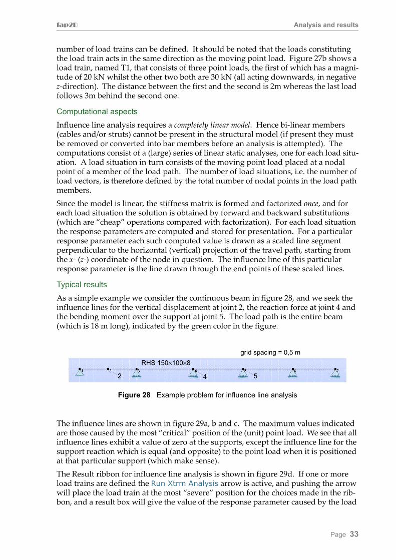
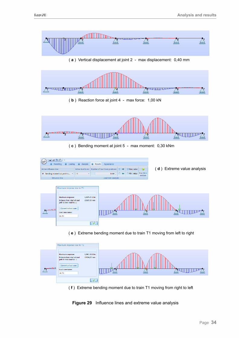
As a simple example we consider the continuous beam in figure 28, and we seek the influence lines for the vertical displacement at joint 2, the reaction force at joint 4 and the bending moment over the support at joint 5. The load path is the entire beam (which is 18 m long), indicated by the green color in the figure.
The influence lines are shown in figure 29a, b and c. The maximum values indicated are those caused by the most “critical” position of the (unit) point load. We see that all influence lines exhibit a value of zero at the supports, except the influence line for the support reaction which is equal (and opposite) to the point load when it is positioned at that particular support (which make sense).The Result ribbon for influence line analysis is shown in figure 29d. If one or more load trains are defined the Run Xtrm Analysis arrow is active, and pushing the arrow will place the load train at the most “severe” position for the choices made in the rib-bon, and a result box will give the value of the response parameter caused by the load
grid spacing = 0,5 m
Figure 28 Example problem for influence line analysis
2 4 5
RHS 150×100×8
Page 33
fap2D Analysis and results
( b ) Reaction force at joint 4 - max force: 1,00 kN
( a ) Vertical displacement at joint 2 - max displacement: 0,40 mm
( c ) Bending moment at joint 5 - max moment: 0,30 kNm
Figure 29 Influence lines and extreme value analysis
( d ) Extreme value analysis
( e ) Extreme bending moment due to train T1 moving from left to right
( f ) Extreme bending moment due to train T1 moving from right to left
Page 34

fap2D Analysis and results
train when in this position. Figures 29 e and f show the results for the bending moment at joint 5 when the “train” moves from left to right (e) and when it moves from right to left (f). Depending on the “train”, these two values need not (as shown by this example) be the same (although the difference here is very small).
Page 35
fap2D Analysis and results
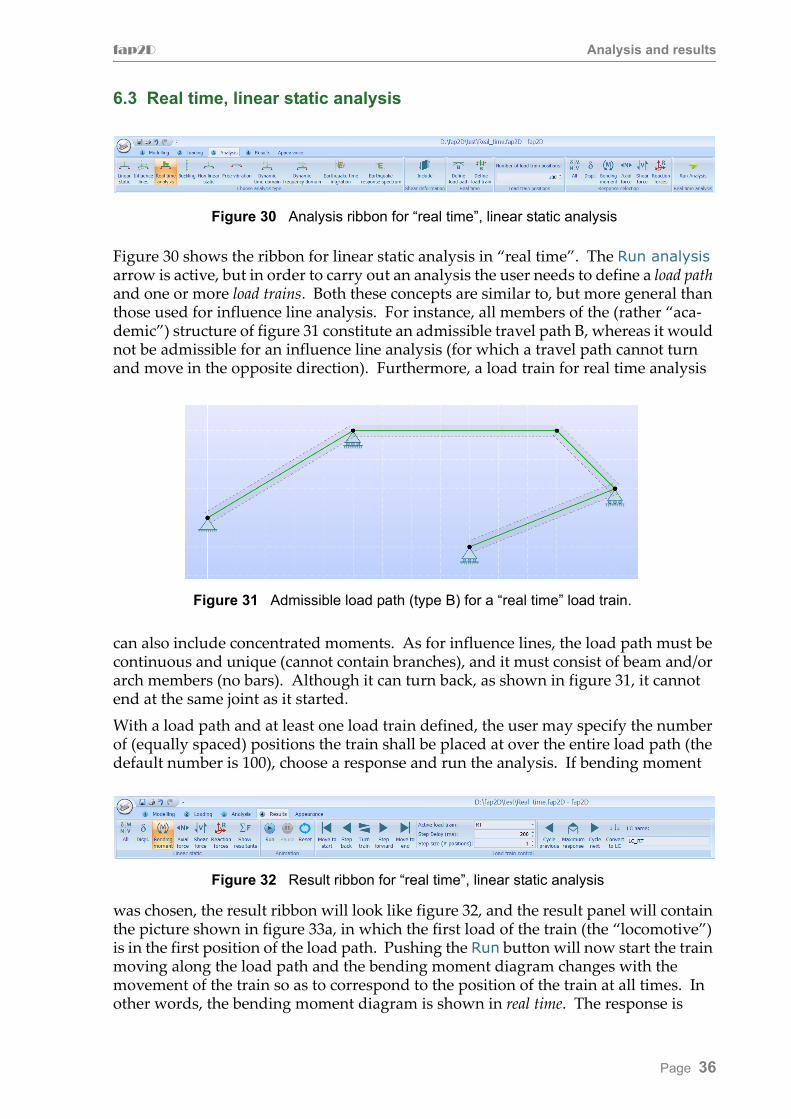
6.3 Real time, linear static analysis
Figure 30 shows the ribbon for linear static analysis in “real time”. The Run analysis arrow is active, but in order to carry out an analysis the user needs to define a load path and one or more load trains. Both these concepts are similar to, but more general than those used for influence line analysis. For instance, all members of the (rather “aca-demic”) structure of figure 31 constitute an admissible travel path B, whereas it would not be admissible for an influence line analysis (for which a travel path cannot turn and move in the opposite direction). Furthermore, a load train for real time analysis
can also include concentrated moments. As for influence lines, the load path must be continuous and unique (cannot contain branches), and it must consist of beam and/or arch members (no bars). Although it can turn back, as shown in figure 31, it cannot end at the same joint as it started.With a load path and at least one load train defined, the user may specify the number of (equally spaced) positions the train shall be placed at over the entire load path (the default number is 100), choose a response and run the analysis. If bending moment
was chosen, the result ribbon will look like figure 32, and the result panel will contain the picture shown in figure 33a, in which the first load of the train (the “locomotive”) is in the first position of the load path. Pushing the Run button will now start the train moving along the load path and the bending moment diagram changes with the movement of the train so as to correspond to the position of the train at all times. In other words, the bending moment diagram is shown in real time. The response is
Figure 30 Analysis ribbon for “real time”, linear static analysis
Figure 31 Admissible load path (type B) for a “real time” load train.
Figure 32 Result ribbon for “real time”, linear static analysis
Page 36

fap2D Analysis and results
scaled with respect to the maximum response. Similar for the other responses. Once the train is moving it may be stopped at any time by pushing the Pause button (that becomes active once the train is moving); it may be started again (by pushing the Run button) or it may be moved one step forward or back by pushing the appropriate but-tons. It is also possible to move the train directly to the end or back to the start of the load path, and the train direction may be changed whenever the train is stationary.The speed of the train is controlled by the Step Delay.Pushing the Maximum response button will take the train to the position where it causes the maximum response, see figure 33b. This position is already known when the user moves from the Analysis ribbon (having pushed the Run analysis button) to the Result ribbon; this enables the program to scale the response with respect to its maximum value. Sometimes several positions may cause the same maximum response; the two cycle buttons will reveal if this is the case.Any stationary position of the train may be made into a named load case (LC).
Figure 33 Real time bending moments
( a ) train in start position ( b ) train in “maximum” position
Page 37

fap2D Analysis and results
6.4 Linearized buckling analysis
Figure 34 shows the ribbon for linearized buckling analysis. The Run analysis arrow
is active, but if you have not made a visit to the Loading button, a push on Run analy-sis will cause the dialog box in figure 35a to appear; this is the same dialog box that the Loading button will open. Here you will have to make some assumptions and then specify the loading. You can assume all loading to be variable or you can assume both variable and constant loading; the significance of this choice is explained below, but the upshot is that the computed buckling factors only apply to the variable loading.
Having made this choice, the spatial load combination(s) need(s) to be specified. The number of modes may be specified in the ribbon (5 is the default choice) as may inclu-sion of shear deformations.
Computational aspects
The total loading, R, may consist of a constant part, Rc , and a variable part, pRv . The variable part is assumed to vary proportionally with a multiplier p, that is
(1)
where Rv is the nominal part of the variable loading (expressed by a spatial load com-bination). It should be noted that the variable part, Rv , can only contain external loading (no prescribed displacements or initial strains).Linearized buckling analysis is concerned with the 2nd order stiffness matrix
(2)
where Km is the material stiffness and KG , which is a function of the axial forces P, is
Figure 34 Analysis ribbon for linearized buckling analysis
Figure 35 Load options (a) and typical buckling mode (b)
(a) Load option dialog box (b) Typical buckling mode (mode #2)
buckling factor
= 41,35
R Rc pRv+=
K2 Km KG P( )–=
Page 38

fap2D Analysis and results
the geometric stiffness. The minus sign in equation (2) assumes the axial forces taken positive as compression (which is a common convention in buckling analysis). The material stiffness is identical to the ordinary 1st order stiffness K0 , modified with respect to bi-linear bar elements. Shear deformations may be included in K0 .The geometric stiffness matrix may be expressed as
(3)
where KGc is the geometric stiffness due to the axial forces (Pc) caused by Rc acting alone, and KGv is the geometric stiffness due to the axial forces (Pv) caused by the nominal Rv acting alone. Hence
(4)
where K1 is the material stiffness modified with respect to the geometric stiffness effects of the constant part of the loading, that is
(5)
Buckling is now defined as a state for which K2 becomes singular. For a singular K2 the homogeneous system of equations
(6)
has non-trivial solutions (pi ,qi). Equation (6) represents a general, symmetric eigen-problem. This problem is (by default) solved by so-called subspace iteration. However, it is possible to choose a truncated Lanczos method for the eigenvalue extraction: go to the Application menu (push the button in the top left-hand corner of the screen) and push Settings > Local > Computational model and choose eigenvalue algorithm. The separation of the loading into a constant (Rc) and a variable part (Rv), which is controlled by the user (see figure 35a), may be useful in many practical situations where certain loading is always constant (e.g. dead load). The buckling factor then indicates by how much the variable part of the loading can be increased before the structure becomes unstable, which is normally the most interesting question.
Typical results
The only results from a buckling analysis are the buckling mode shapes and the corre-sponding buckling factor (which is the factor by which the variable part of the loading must be multiplied in order to cause the structure to “buckle” in the corresponding mode shape). In figure 35b is shown the 2nd buckling mode for the frame of figure 19 subjected to the loading of figure 22 (which is all variable). The first buckling mode is simple “Euler buckling” of column B-D, for which the buckling factor is somewhat smaller than that in figure 35b, namely 32,11.
KG KGc pKGv+=
K2 K0 KGc– pKGv– K1 pKGv–= =
K1 K0 KGc–=
K2q K1 pKGv–( )q 0= =
Page 39

fap2D Analysis and results
6.5 Nonlinear static analysis
Figure 36 shows the ribbon for nonlinear static analysis. The Run analysis arrow is
active, but if the user pushes it prior to having paid a visit to the Load history, the dia-log box shown in figure 37a will appear; this is the same dialog box that the Load his-tory button will open. However, the user may first consider to impose some kind of geometrical imperfection; default is no such imperfections. The shape imperfection button launches the dialog box in figure 37b. A global shape imperfection may be
imposed, the form of which may be in the shape of a buckling mode shape due to a specific load combination or in the shape of the static deformations due to a specified load combination. In either case the user must provide the maximum “amplitude” (in mm). Instead of, or in addition to, the global imperfection, local imperfections in the shape of half sine waves (with amplitudes equal to L/n) may be specified for selected beam (compression) members.With reference to the dialog box in figure 37a two “types” of loading may be speci-fied, a constant loading (Rc) applied in full at “time” zero (λ = 0) and a variable loading (Rv) applied gradually, from zero to full magnitude, in a certain number (= n) of equal increments. The user may specify the one or the other, or both in combination. In the latter case some of the loading is applied at time zero, and maintained constant throughout, whereas the rest of the loading is applied gradually, in equal increments. Both types of loading are defined in terms of a spatial load combination which may already be defined or it may be defined by selecting Add/edit in the appropriate drop down menu.
Figure 36 Analysis ribbon for nonlinear static analysis
(a) (b)
Figure 37 Dialog boxes for geometric load history (a) and imperfection (b)
Page 40
fap2D Analysis and results
Computational aspects
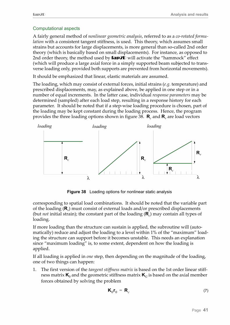
A fairly general method of nonlinear geometric analysis, referred to as a co-rotated formu-lation with a consistent tangent stiffness, is used. This theory, which assumes small strains but accounts for large displacements, is more general than so-called 2nd order theory (which is basically based on small displacements). For instance, as opposed to 2nd order theory, the method used by fap2D will activate the “hammock” effect (which will produce a large axial force in a simply supported beam subjected to trans-verse loading only, provided both supports are prevented from horizontal movements).It should be emphasized that linear, elastic materials are assumed.The loading, which may consist of external forces, initial strains (e.g. temperature) and prescribed displacements, may, as explained above, be applied in one step or in a number of equal increments. In the latter case, individual response parameters may be determined (sampled) after each load step, resulting in a response history for each parameter. It should be noted that if a step-wise loading procedure is chosen, part of the loading may be kept constant during the loading process. Hence, the program provides the three loading options shown in figure 38. Rc and Rv are load vectors
corresponding to spatial load combinations. It should be noted that the variable part of the loading (Rv) must consist of external loads and/or prescribed displacements (but not initial strain); the constant part of the loading (Rc) may contain all types of loading.If more loading than the structure can sustain is applied, the subroutine will (auto-matically) reduce and adjust the loading to a level within 1% of the “maximum” load-ing the structure can support before it becomes unstable. This needs an explanation since “maximum loading” is, to some extent, dependent on how the loading is applied.If all loading is applied in one step, then depending on the magnitude of the loading, one of two things can happen:1. The first version of the tangent stiffness matrix is based on the 1st order linear stiff-
ness matrix K0 and the geometric stiffness matrix KG is based on the axial member forces obtained by solving the problem
(7)
λ λ λ
loading loading loading
Rc Rv
Rc
Rv
Figure 38 Loading options for nonlinear static analysis
K0r0 Rc=
Page 41
fap2D Analysis and results
If the loading Rc is sufficiently large, the matrix K0 - KG may be indefinite, and this is taken as an indication that Rc is more than the structure can support. The load-ing is halved and the procedure starts all over again. If this results in a positive definite matrix, the program will iterate until the unbalanced forces are suffi-ciently small, and a new load increment, which is half of the previous loading is applied. A new tangent matrix is established and tested for positive definiteness. If positive definite equilibrium, iterations are carried out and a new load incre-ment, which is half of the previous one is applied; if not positive definite the pro-gram backs up to the last equilibrium position and halve the load increment once again before the procedure is repeated. This goes on until an equilibrium position is obtained for a loading within 1% of the smallest (total) load that cause an indef-inite tangent stiffness matrix. It follows that this loading will be smaller than the loading Rc , applied originally, if this loading caused indefiniteness in the first step.
2. If the loading Rc does not cause the tangent stiffness matrix to become indefinite or negative definite, the program will carry out equilibrium iterations with full loading on the structure, which involves updating the geometry, until the unbal-anced forces are sufficiently small.
If the same total loading is applied as a variable load in, say 20, equal increments, the structure may well be capable of sustaining considerable more load than if the same load was applied in just one step. This will be demonstrated by a simple example below, and it has to do with the fact that gradual loading facilitates force redistri-bution to take place which in turn may give the structure more apparent strength. Apparent because material failure will most likely occur long before the “maximum stability load” is attained. This discussion may therefore be a bit academic.
Typical results
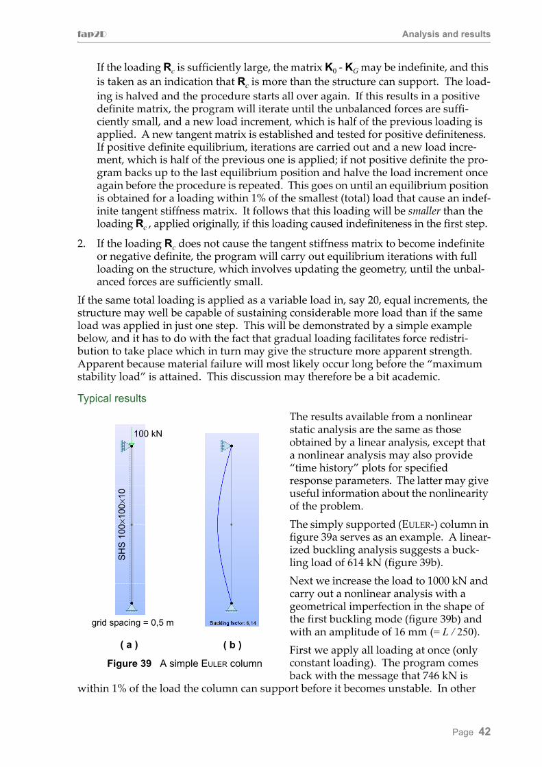
The results available from a nonlinear static analysis are the same as those obtained by a linear analysis, except that a nonlinear analysis may also provide “time history” plots for specified response parameters. The latter may give useful information about the nonlinearity of the problem.The simply supported (EULER-) column in figure 39a serves as an example. A linear-ized buckling analysis suggests a buck-ling load of 614 kN (figure 39b).Next we increase the load to 1000 kN and carry out a nonlinear analysis with a geometrical imperfection in the shape of the first buckling mode (figure 39b) and with an amplitude of 16 mm (= L / 250).First we apply all loading at once (only constant loading). The program comes back with the message that 746 kN is
within 1% of the load the column can support before it becomes unstable. In other
grid spacing = 0,5 m
100 kN
SH
S 1
00×1
00×1
0
Figure 39 A simple EULER column
( a ) ( b )
Page 42

fap2D Analysis and results
words, a starting load of 1000 kN clearly caused a negative definite tangent stiffness. The results from this analysis are shown in figure 40.
We repeat the analysis, but this time we apply the loading gradually, in 50 equal incre-ments. This time the results, shown in figure 41, are obtained for the full load (1000 kN).
Max. displ. Max. axial force Max. bending moment Max. shear force
1448 mm 746 kN 1005 kNm 709 kN
Figure 40 Results for the EULER column subjected to 1000 kN applied at once
Max. displ. Max. axial force Max. bending moment Max. shear force
2954 mm 999 kN 1607 kNm 1000 kN
Figure 41 Results for the EULER column subjected to 1000 kN applied incrementally(50 load increments)
Page 43

fap2D Analysis and results
When comparing results it should be kept in mind that they are normalized results. This is particularly important for the displacement which clearly is not drawn to scale in figures 40 and 41. If we, instead of Show all click the Displacement button and then the Tδ (true displacement) button in the toolbox, a completely different picture appears, see figure 42. And now the tensile axial forces in figure 41 make sense.
The results of figures 40, 41 and 42 are of more academic than practical interest. On closer inspection we find that stresses are of magnitude 15 000 MPa; hence material failure will have occurred long before the displacements of these figures are attained.The lesson here is that loads that can possibly vary should preferably be applied incrementally, particularly if stress redistribution can take place.Another useful result available after a nonlinear analysis, for which the loading is applied step-by-step, is the “time history” of defined response parameters. Figure 43 shows how the horizontal displacement of the mid-point of the column varies with “time” λ (which is really a measure of the external load), for the loading case of figure 41. This type of result requires (a) that response parameters have been defined and
(b) that the load is applied incrementally, preferably with a significant number of load increments.
Figure 42 True displacements
( a ) P = 746 kN (fig. 30) ( b ) P = 1000 kN (fig. 31)
Figure 43
Horizontal displacementvs
“tilme” or loading
P = 1000 kNPE
Page 44

fap2D Analysis and results
6.6 Free, undamped vibration analysis
Figure 44 shows the ribbon for free vibration analysis. The Run analysis arrow is
active, and if pushed a free vibration analysis will be carried out for default choices of stiffness and mass. Figure 45 shows the dialog boxes “behind” the Stiffness and Mass buttons, respectively. We see that it is possible to modify the structural stiffness by
including the geometric stiffness, due to a particular load combination, before carry-ing out the free vibration analysis, see next section. An example of this would be to determine the free vibration characteristics of a structure subjected to all dead load, e.g. a bridge. For structures with cable members this may make a significant differ-ence. The default choice for the mass representation is lumped mass, the obvious choice for the modelling philosophy of fap2D.The user also needs to specify the number of mode shapes to be determined (default is 5) and where on the frequency axis the eigenvalues shall be extracted, defined by the so-called shift value σ (default is σ = 0). More about this below.
Computational aspects
The numerical problem to solve is the general, symmetric eigenproblem
(8)
where K is the stiffness matrix, M is the mass matrix, ω is the circular frequency of the free vibration ( is the eigenvalue of the problem) and q is the corresponding mode of vibration (eigenvector). Normally the program will determine a limited number (n) of the lowest eigenvalues and corresponding eigenvectors (mode shapes), so-called eigenpairs (λi ,qi), that satisfy eqn. (8). If a non-zero shift (σ) is specified, the modified problem
(9)
Figure 44 Analysis ribbon for free vibration analysis
Figure 45 Stiffness and mass settings for free vibration analysis
K ω2M–( )q 0=
λ ω2=
Kσ μM–( )q 0=
Page 45

fap2D Analysis and results
is solved, where and . The problem is equivalent to finding n roots of the characteristic polynomial in the vicinity of σ on the frequency axis, see figure 46.
The eigenvalue problem of eqn. (8) is (by default) solved by so-called subspace itera-tion. However, as for linearized buckling, it is possible to choose a truncated Lanczos method for the eigenvalue extraction: go to the Application menu (push the button in the top left-hand corner of the screen) and push Settings > Local > Computational model and choose eigenvalue algorithm.
Results
The only results from a free vibration analysis are the mode shapes and correspon-ding frequencies (in Hz). Displacement plots very similar to the buckling mode shapes are produced, accompanied by the corresponding frequency. For the frame in figure 19 the first (or lowest) mode shape is very similar to the second buckling mode shown in figure 35b, its frequency is 6,06 Hz.A useful feature is animation of the free vibration mode shapes; start and pause but-tons are available in the Results ribbon page.
μ λ σ–= Kσ K σM–=
p(λ) = det(K - λiM)
λσ (shift)
n eigenvalues (roots of p(λ))
NOTE: λ = ω2
Figure 46 Schematic presentation of the free vibration eigenvalue problem
Page 46
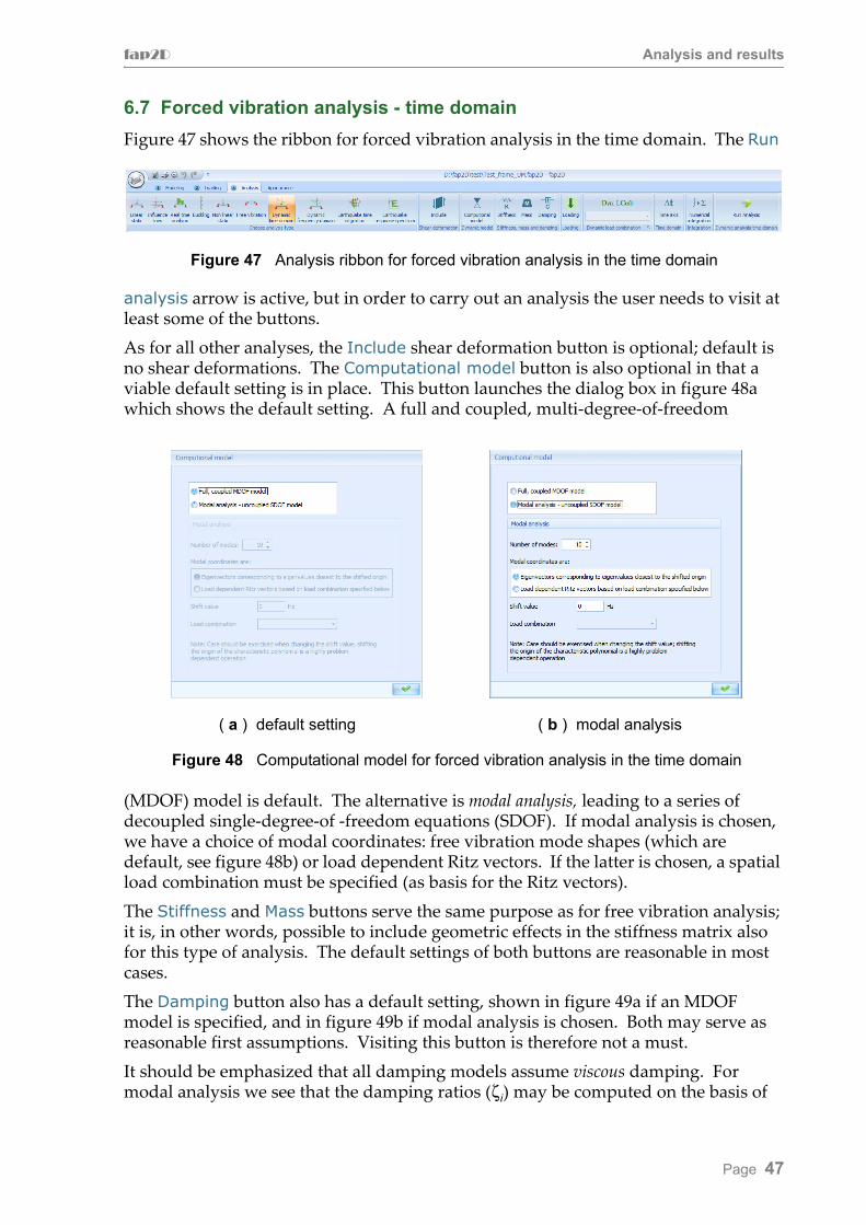
fap2D Analysis and results
6.7 Forced vibration analysis - time domain
Figure 47 shows the ribbon for forced vibration analysis in the time domain. The Run
analysis arrow is active, but in order to carry out an analysis the user needs to visit at least some of the buttons.As for all other analyses, the Include shear deformation button is optional; default is no shear deformations. The Computational model button is also optional in that a viable default setting is in place. This button launches the dialog box in figure 48a which shows the default setting. A full and coupled, multi-degree-of-freedom
(MDOF) model is default. The alternative is modal analysis, leading to a series of decoupled single-degree-of -freedom equations (SDOF). If modal analysis is chosen, we have a choice of modal coordinates: free vibration mode shapes (which are default, see figure 48b) or load dependent Ritz vectors. If the latter is chosen, a spatial load combination must be specified (as basis for the Ritz vectors).The Stiffness and Mass buttons serve the same purpose as for free vibration analysis; it is, in other words, possible to include geometric effects in the stiffness matrix also for this type of analysis. The default settings of both buttons are reasonable in most cases.The Damping button also has a default setting, shown in figure 49a if an MDOF model is specified, and in figure 49b if modal analysis is chosen. Both may serve as reasonable first assumptions. Visiting this button is therefore not a must. It should be emphasized that all damping models assume viscous damping. For modal analysis we see that the damping ratios (ζi) may be computed on the basis of
Figure 47 Analysis ribbon for forced vibration analysis in the time domain
Figure 48 Computational model for forced vibration analysis in the time domain
( a ) default setting ( b ) modal analysis
Page 47
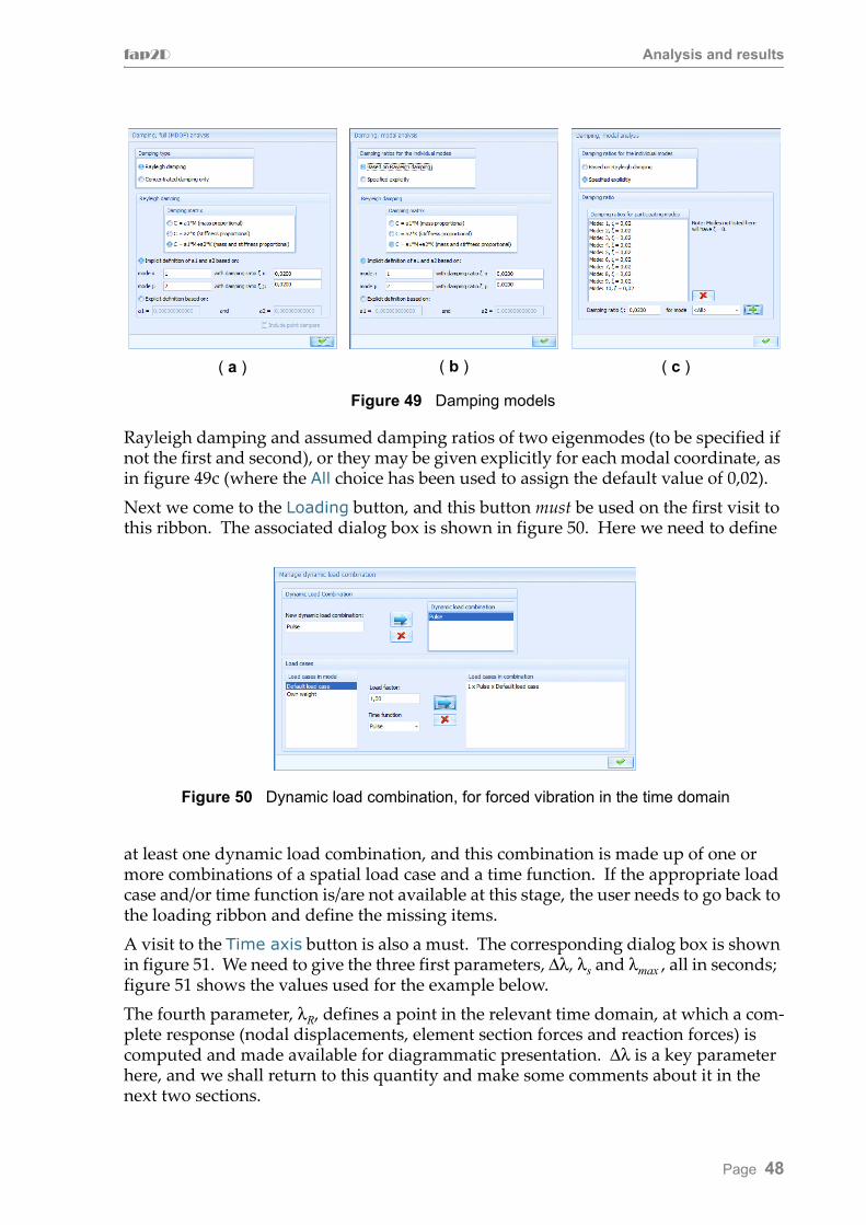
fap2D Analysis and results
Rayleigh damping and assumed damping ratios of two eigenmodes (to be specified if not the first and second), or they may be given explicitly for each modal coordinate, as in figure 49c (where the All choice has been used to assign the default value of 0,02).Next we come to the Loading button, and this button must be used on the first visit to this ribbon. The associated dialog box is shown in figure 50. Here we need to define
at least one dynamic load combination, and this combination is made up of one or more combinations of a spatial load case and a time function. If the appropriate load case and/or time function is/are not available at this stage, the user needs to go back to the loading ribbon and define the missing items.A visit to the Time axis button is also a must. The corresponding dialog box is shown in figure 51. We need to give the three first parameters, Δλ, λs and λmax , all in seconds; figure 51 shows the values used for the example below.The fourth parameter, λR, defines a point in the relevant time domain, at which a com-plete response (nodal displacements, element section forces and reaction forces) is computed and made available for diagrammatic presentation. Δλ is a key parameter here, and we shall return to this quantity and make some comments about it in the next two sections.
Figure 49 Damping models
( a ) ( b ) ( c )
Figure 50 Dynamic load combination, for forced vibration in the time domain
Page 48
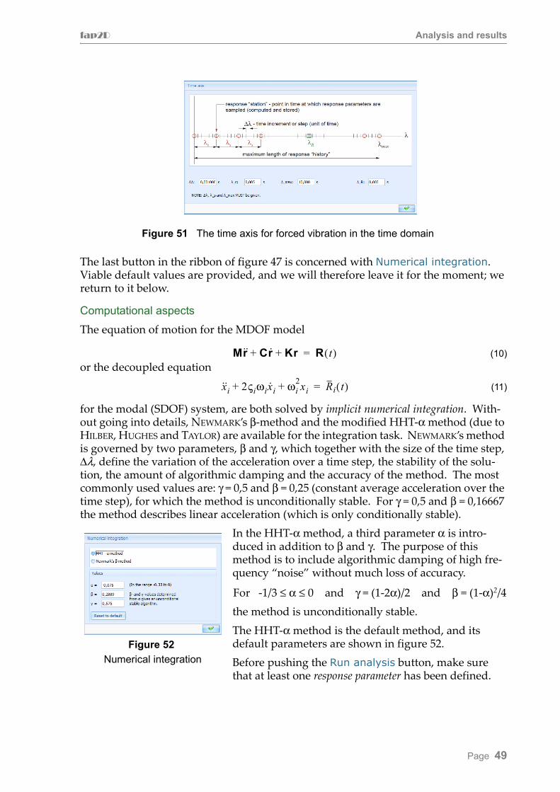
fap2D Analysis and results
The last button in the ribbon of figure 47 is concerned with Numerical integration. Viable default values are provided, and we will therefore leave it for the moment; we return to it below.
Computational aspects
The equation of motion for the MDOF model
(10)
or the decoupled equation
(11)
for the modal (SDOF) system, are both solved by implicit numerical integration. With-out going into details, NEWMARK’s β-method and the modified HHT-α method (due to HILBER, HUGHES and TAYLOR) are available for the integration task. NEWMARK’s method is governed by two parameters, β and γ, which together with the size of the time step, Δλ, define the variation of the acceleration over a time step, the stability of the solu-tion, the amount of algorithmic damping and the accuracy of the method. The most commonly used values are: γ = 0,5 and β = 0,25 (constant average acceleration over the time step), for which the method is unconditionally stable. For γ = 0,5 and β = 0,16667 the method describes linear acceleration (which is only conditionally stable).
In the HHT-α method, a third parameter α is intro-duced in addition to β and γ. The purpose of this method is to include algorithmic damping of high fre-quency “noise” without much loss of accuracy.
For -1/3 ≤ α ≤ 0 and γ = (1-2α)/2 and β = (1-α)2/4the method is unconditionally stable.The HHT-α method is the default method, and its default parameters are shown in figure 52.Before pushing the Run analysis button, make sure that at least one response parameter has been defined.
Figure 51 The time axis for forced vibration in the time domain
Mr·· Cr· Kr+ + R t( )=
x··i 2ςiωix·
i ωi2xi+ + Ri t( )=
Figure 52
Numerical integration
Page 49

fap2D Analysis and results
Typical results
In order to demonstrate the capabilities of this type of analysis we consider a very simple problem, namely the simply supported steel beam shown in figure 53a. The beam has a parametric cross section shown in figure 53 b, and it is subjected to a verti-cal point load of 10 kN at the middle of the beam. The time variation of the load is a “pulse” of 1,0 s duration shown in figure 54. Ten consecutive periods of this pulse is considered as the (total) time function.
Back to the time axis parameters, see figure 51, we now (somewhat arbitrarily) specify the time increment to be Δλ = 0,001 s. We sample the response parameter, the vertical displacement of the loaded mid-point, at each 5th time increment, that is λs = 0,005 s. The duration of the response range is set equal to that of the loaded period, hence
10 kN
8 m 8 m
( a )
( b ) beam cross section
Figure 53 Example problem
Figure 54 Time function “Pulse”
Page 50

fap2D Analysis and results
λmax = 10,0 s. The last parameter, λR, we leave alone, and its value of zero indicates no system results. With these parameters and the default choice for the other buttons, i.e., an MDOF computational model, only material stiffness, lumped mass model, Rayleigh damping based on a damping ratio ζ = 0,02 in the two lowest natural modes, and an HHT-α integration scheme with the default values of figure 52, the vertical dis-placement of the beam mid-point as a function of time is shown in figure 55a.
We repeat the analysis with one change: instead of the MDOF model we now use modal analysis with the 10 lowest modes of free vibration as modal coordinates. Other-wise the same assumptions as before. The time-history plot for this model is shown in
( a )
Full, MDOF model
( b )
Modal analysis with the 10 lowest free vibration modes as modal cooordinates
Figure 55 Time-history plots of the vertical displacement at the mid-point of the beam
( c )
Modal analysis with 10 load dependent Ritz vectors as modal cooordinates
43,71 35,04
43,70 35,04
43,71 35,04
Page 51

fap2D Analysis and results
figure 55b.We repeat the analysis yet again; still modal analysis, but this time we use 10 load dependent Ritz vectors as modal coordinates. The point load is used as loading for the Ritz vectors. The time history plot for this model is shown in figure 55c.We see that with the resolution of the plots in figure 55 it is impossible to distinguish the three plots, and two distinct values are practically the same for all three methods. For this simple example that is hardly surprising. Another comment is that the time increment used in this case (0,001s) is probably unnecessarily small. This can easily be established by a simple sensitivity analysis in which results obtained with different values of the time increment (Δλ) are compared. However, with the current compu-tational power of a standard PC, some “overkill” is probably justified.The type of “x-y plot” shown in figure 55 is used extensively in fap2D. It is possible to show some response values on the plot by checking the Show values on graph box, see figure 56a. More useful, however, is the possibility to zoom in on a specific time interval, and show the response at specific points in time, see figure 56b. The latter is accomplished by (left) clicking the graph view and then use the scroll wheel to zoom in and out. The black circle is moved along the graph with the cursor (the response and time values update dynamically).
( a )
Show values on graph
( b )
Zoom in on a specifictime interval
Figure 56 Time-history plots of the vertical displacement at the mid-point of the beam
Page 52

fap2D Analysis and results
6.8 Forced vibration analysis - frequency domain
Figure 57 shows the ribbon for forced vibration analysis in the time domain. The Run
analysis arrow is active, but in order to carry out an analysis the user needs to visit the Harmonic or Periodic load button which launches the dialog box in figure 58a. There are three load options in the frequency domain:1. One harmonic load combination where all contributing spatial load cases have a
harmonic variation with the same (load) frequency. However, the various contri-buting load cases may have different phase angles.This is the program’s default choice, see figure 58a.The results from this analysis are the following steady state results for all nodal displacements and element section forces: amplitude values, dynamic amplification or dynamic load factors (DLF) and phase angles.
2. One spatial load combination with harmonic variation applied for a series of frequencies, see figure 58b. The user needs to specify a spatial load combination, a frequency range and the number of (equally spaced) frequencies within the range for which steady state response of all specified response parameters are com-puted.The results are, for each specified response parameter, frequency plots of: the amplitude values, the dynamic load factors (DLF) and the phase angles.
3. One periodic, but non-harmonic load combination, see figure 58c. Here the user need to specify a spatial load combination, a time function defining one period of loading plus some information used by the program when approximating the load by a FOURIER series of harmonic components. Two parameters control the FOURIER series expansion, the maximum number of Fourier terms (default value is 75) and a tolerance parameter (default value is 0,05) that control the actual num-ber of terms used. The user should not change these numbers before an inspec-tion of the time function approximation has been made; this approximation is available after the analysis has been carried out, more below.The user also has to provide the number of time increments in one period - the program will determine the (steady state) response at each time increment.The main results provided are the steady state response curves over one time period for all specified response parameters; hence, this type of analysis is not relevant unless at least one response parameter has been specified (at a joint). The only other piece of information available after a successful analysis is a plot of the (FOUIER) approximation of the time function.
Computational aspects
The problem is solved by the frequency response method using, as for the time domain,- the full, coupled multi-degree-of-freedom (MDOF) system,
Figure 57 Analysis ribbon for forced vibration analysis in the frequency domain
Page 53

fap2D Analysis and results
( a )
Harmonic loading with one load frequency
( b )
Harmonic loading with several load frequencies
( c )
Periodicnon-harmonic loading
Figure 58 Load options in the frequency domain
Page 54

fap2D Analysis and results
or- superposition of a system of decoupled, single-degree-of-freedom (SDOF)
equations obtained by modal analysis; both eigenvectors and so-called load dependent Ritz vectors may be used as modal coordinates.
Representation of stiffness, mass and damping is also the same as in the time domain.The problem is to find the solution of
(12)
Ω is the frequency of the applied harmonic loading. We seek the particular solution of eqn. (12), that is the so-called steady state solution
(13)
which has the same frequency as the loading. A tilde (~) on top of a symbol denotes a complex quantity. Substituting eqn. (13) into eqn. (12) yields:
(14)
or
(15)
where
(16)
is the complex dynamic stiffness matrix. The solution of eqn. (15) gives the complex response vector . An arbitrary response component (dof number j) may be expressed as
(17)
where
(18)
whose real and imaginary components are
(19)
Here
(20)
is the amplitude value of the response, and
(21)
its phase angle. In order to determine the dynamic amplification, also referred to as the dynamic load factor (DLF), defined as the ratio between dynamic and static response, the static response needs to be solved. This is accomplished by solving eqn. (15) forΩ = 0, that is
(22)
Mr·· Cr· Kr+ + R Ω( ) R̃eiΩt= =
r r̃eiΩt=
Ω2Mr̃– iΩCr̃ Kr̃+ + R̃=
K̃r̃ R̃=
K̃ K Ω2M– iΩC+=
r̃
rj rj0ei Ωt βj+( )
r̃jeiΩt= =
r̃j rj0eiβj rjR irjI+= =
rjR rj0 βj and rjIcos rj0 βjsin= =
rj0 rjR2
rjI2+=
βj
rjI
rjR------
atan=
K rRs
irIs+( ) RR iRI+=
Page 55
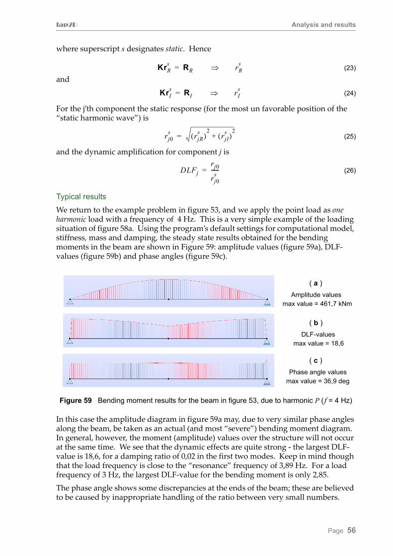
fap2D Analysis and results
where superscript s designates static. Hence
(23)
and
(24)
For the j’th component the static response (for the most un favorable position of the “static harmonic wave”) is
(25)
and the dynamic amplification for component j is
(26)
Typical results
We return to the example problem in figure 53, and we apply the point load as one harmonic load with a frequency of 4 Hz. This is a very simple example of the loading situation of figure 58a. Using the program’s default settings for computational model, stiffness, mass and damping, the steady state results obtained for the bending moments in the beam are shown in Figure 59: amplitude values (figure 59a), DLF-values (figure 59b) and phase angles (figure 59c).
In this case the amplitude diagram in figure 59a may, due to very similar phase angles along the beam, be taken as an actual (and most “severe”) bending moment diagram. In general, however, the moment (amplitude) values over the structure will not occur at the same time. We see that the dynamic effects are quite strong - the largest DLF-value is 18,6, for a damping ratio of 0,02 in the first two modes. Keep in mind though that the load frequency is close to the “resonance” frequency of 3,89 Hz. For a load frequency of 3 Hz, the largest DLF-value for the bending moment is only 2,85.The phase angle shows some discrepancies at the ends of the beam; these are believed to be caused by inappropriate handling of the ratio between very small numbers.
KrRs
RR rRs=
KrIs
RI rIs=
rj0s
rjRs( )
2rjI
s( )2
+=
DLFj
rj0
rj0s
------=
( a )
Amplitude valuesmax value = 461,7 kNm
( b )
DLF-valuesmax value = 18,6
( c )
Phase angle valuesmax value = 36,9 deg
Figure 59 Bending moment results for the beam in figure 53, due to harmonic P ( f = 4 Hz)
Page 56

fap2D Analysis and results
Results similar to those of figure 59 are available also for displacement, axial force and shear force.Next, we apply the same point load, but this time as a series of harmonic load cases with 140 different frequencies equally spaced between 1,5 and 5 Hz (a simple example of the loading situation of figure 58b). Results are available only for specified response parameters of which we have one, the transverse displacement under the load. Again we use the program’s default settings for computational model, stiffness, mass and damping, and the steady state results obtained for the transverse displace-ment under the load are shown in Figure 60 as plots along the frequency axis of the amplitude values (figure 60a), DLF-values (figure 60b) and phase angles (figure 60c). As expected, both amplitude and DLF peak at the lowest natural frequency (3,89 Hz).
Finally we subject the beam to a point load with a periodic, but non-harmonic variation in time. The load acts, as before, at the mid-point of the beam, and the time variation of one period (which is 1,0 s long) is the “pulse” shown in figure 54.This is a simple example of the loading situation of figure 58c. Again results will only be available for specified response parameters of which we still have defined only one, the transverse displacement under the load. We continue to use the program’s default settings for computational model, stiffness, mass and damping. Also for the parameters controlling the FOURIER series approximation we use the default values
( a ) Amplitude
( b ) DLF (dynamic amplification)
( c ) Phase angle
Figure 60 Transverse mid-point displacement due to a harmonic point load P (= 10 kN)
Page 57
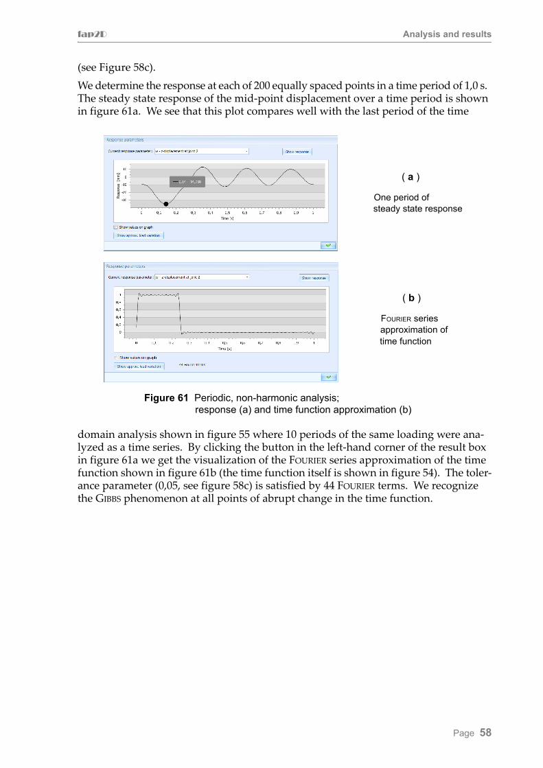
fap2D Analysis and results
(see Figure 58c).We determine the response at each of 200 equally spaced points in a time period of 1,0 s. The steady state response of the mid-point displacement over a time period is shown in figure 61a. We see that this plot compares well with the last period of the time
domain analysis shown in figure 55 where 10 periods of the same loading were ana-lyzed as a time series. By clicking the button in the left-hand corner of the result box in figure 61a we get the visualization of the FOURIER series approximation of the time function shown in figure 61b (the time function itself is shown in figure 54). The toler-ance parameter (0,05, see figure 58c) is satisfied by 44 FOURIER terms. We recognize the GIBBS phenomenon at all points of abrupt change in the time function.
Figure 61 Periodic, non-harmonic analysis;response (a) and time function approximation (b)
( a )
One period of steady state response
( b )
FOURIER series approximation oftime function
Page 58

fap2D Analysis and results
6.9 Earthquake analysis
For earthquake analysis fap2D offers two possibilities:• numerical integration of recorded time series of ground acceleration, and• response spectrum analysis.
Time integration
This is a special application of forced vibration in the time domain. Figure 62 shows the ribbon for earthquake time integration The Run analysis arrow is active, but in
order to carry out an analysis the user needs to visit at least one of the buttons, namely the Harmonic loading button which launches the dialog box in figure 63. For each of
three recorded earthquakes three time series are available, two that apply to horizon-tal ground acceleration and one that applies to vertical acceleration. These nine stan-dard time series can be scaled, but otherwise not modified. A horizontal earthquake can be combined with a vertical earthquake, but for the standard earthquakes only time series of the same earthquake can be combined (with individual scale factors). Choose one (or two, but one at a time) earthquake and bring it into the “Excitations” box by pushing the blue arrow. The user can define his or her own earthquakes, either by modifying one of the pre-defined time series, or by importing a time series. In order to do this it is necessary to go back to the Loading page and push the Earthquakes button which launches the dialog box shown in figure 64. In this dialog box, each predefined time series can be inspected along with some of its key information, such as the number of sampling points and the size of the sampling interval (a constant for each individual earthquake series). The earthquake’s dialog box has three buttons that enable the user to manipu-late the time series (Duplicate and edit), import new ones (Import) or export existing
Figure 62 Analysis ribbon for earthquake time integration
Figure 63 Standard (predefined) earthquake time series
Page 59
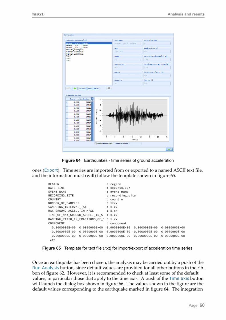
fap2D Analysis and results
ones (Export). Time series are imported from or exported to a named ASCII text file, and the information must (will) follow the template shown in figure 65.
Once an earthquake has been chosen, the analysis may be carried out by a push of the Run Analysis button, since default values are provided for all other buttons in the rib-bon of figure 62. However, it is recommended to check at least some of the default values, in particular those that apply to the time axis. A push of the Time axis button will launch the dialog box shown in figure 66. The values shown in the figure are the default values corresponding to the earthquake marked in figure 64. The integration
Figure 64 Earthquakes - time series of ground acceleration
REGION : regionDATE_TIME : xxxx/xx/xx/EVENT_NAME : event_nameRECORDING_SITE : recording_siteCOUNTRY : countruNUMBER_OF_SAMPLES : xxxxSAMPLING_INTERVAL_(S) : x.xxMAX_GROUND_ACCEL._IN_M/SS : x.xxTIME_OF_MAX_GROUND_ACCEL._IN_S : x.xxDAMPING_RATIO_IN_FRACTIONS_OF_1 : x.xxCOMPONENT : component 0.0000000E-00 0.0000000E-00 0.0000000E-00 0.0000000E-00 0.0000000E-00 -0.0000000E-00 -0.0000000E-00 -0.0000000E-00 -0.0000000E-00 -0.0000000E-00 0.0000000E-00 0.0000000E-00 0.0000000E-00 0.0000000E-00 0.0000000E-00 etc
Figure 65 Template for text file (.txt) for import/export of acceleration time series
Page 60

fap2D Analysis and results
time step (Δλ) is determined by the value of the integer parameter nts (number of time steps per acceleration sampling interval λe); it follows that the largest permissible time step is equal to the sampling interval λe (which is default). Response parameters are (by default) sampled at the same points as the ground acceleration (λs = λe).
Typical results for a simple example
Figure 67 shows a simple concrete tower with a concentrated mass of 50000 kg at the top. The tower has a circular ring section with outer radius re and inner radius ri ;
at the bottom: re = 4000 mm and ri = 3500 mmat the top : re = 1500 mm and ri = 1100 mm
Figure 66 Time axis in case of numerical integration of earthquake ground accelaration
50000 kg
70
000
mm
mode # 1 - f = 1,13 Hz mode # 2 - f = 4,60 Hz
Figure 67 Concrete tower with point mass on top
Page 61
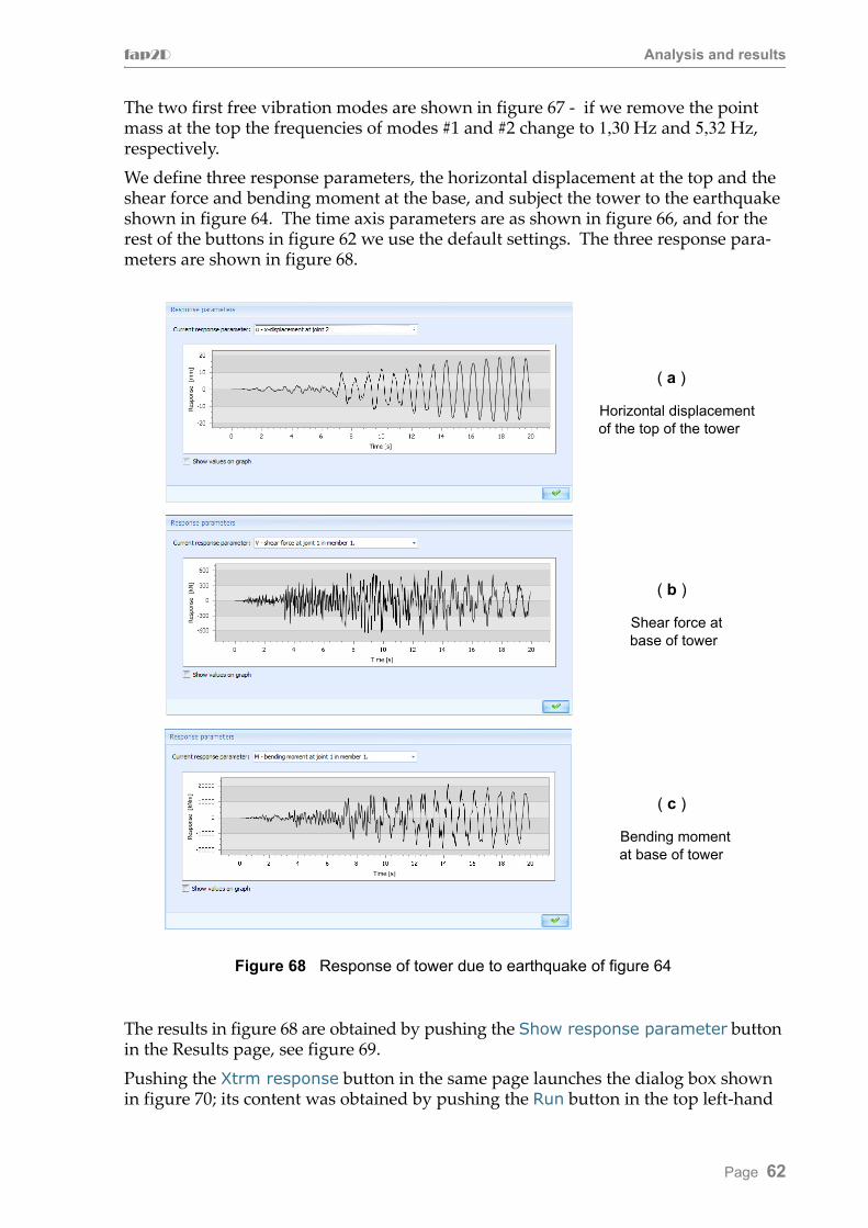
fap2D Analysis and results
The two first free vibration modes are shown in figure 67 - if we remove the point mass at the top the frequencies of modes #1 and #2 change to 1,30 Hz and 5,32 Hz, respectively.We define three response parameters, the horizontal displacement at the top and the shear force and bending moment at the base, and subject the tower to the earthquake shown in figure 64. The time axis parameters are as shown in figure 66, and for the rest of the buttons in figure 62 we use the default settings. The three response para-meters are shown in figure 68.
The results in figure 68 are obtained by pushing the Show response parameter button in the Results page, see figure 69. Pushing the Xtrm response button in the same page launches the dialog box shown in figure 70; its content was obtained by pushing the Run button in the top left-hand
Figure 68 Response of tower due to earthquake of figure 64
( a )
Horizontal displacement of the top of the tower
( b )
Shear force at base of tower
( c )
Bending moment at base of tower
Page 62

fap2D Analysis and results
corner of the dialog box. We see that the maximum values of horizontal displace-ment, shear force and bending moment, and the times of their occurrence match the graphs of figure 68 quite well.
By pushing one of the four Run buttons to the right of the dialog box in figure 70a, the diagram of the corresponding response quantity appears. Figure 70b shows the bend-ing moment diagram (at time 14,28) that emerges after the second Run button is pressed. Diagrams for the other quantities (δ, N and V) are also available at this point in time.We leave it to the user to explore the animation possibilities.
Figure 69 Results ribbon for earthquake time integration
Figure 70 Extreme tower responses due to the applied earthquake
( a ) ( b )
Page 63
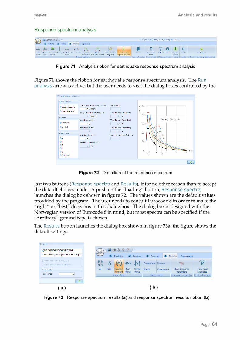
fap2D Analysis and results
Response spectrum analysis
Figure 71 shows the ribbon for earthquake response spectrum analysis. The Run analysis arrow is active, but the user needs to visit the dialog boxes controlled by the
last two buttons (Response spectra and Results), if for no other reason than to accept the default choices made. A push on the “loading” button, Response spectra, launches the dialog box shown in figure 72. The values shown are the default values provided by the program. The user needs to consult Eurocode 8 in order to make the “right” or “best” decisions in this dialog box. The dialog box is designed with the Norwegian version of Eurocode 8 in mind, but most spectra can be specified if the “Arbitrary” ground type is chosen. The Results button launches the dialog box shown in figure 73a; the figure shows the default settings.
Figure 71 Analysis ribbon for earthquake response spectrum analysis
Figure 72 Definition of the response spectrum
Figure 73 Response spectrum results (a) and response spectrum results ribbon (b)
( a ) ( b )
Page 64
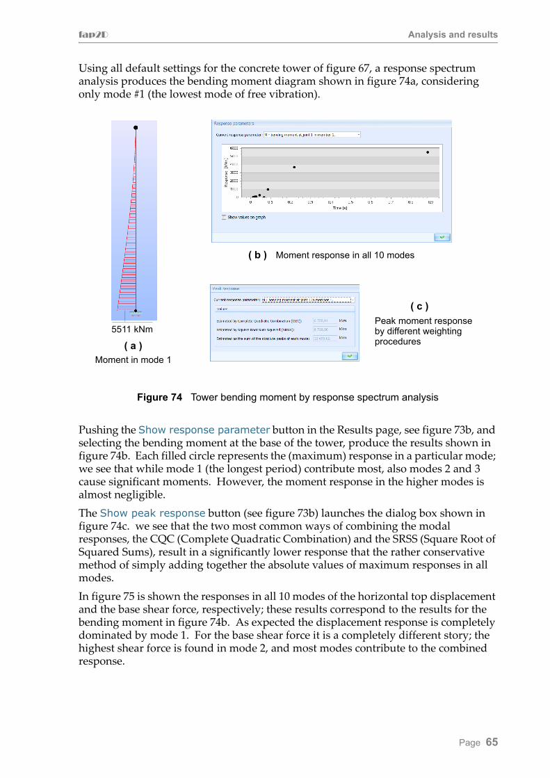
fap2D Analysis and results
Using all default settings for the concrete tower of figure 67, a response spectrum analysis produces the bending moment diagram shown in figure 74a, considering only mode #1 (the lowest mode of free vibration).
Pushing the Show response parameter button in the Results page, see figure 73b, and selecting the bending moment at the base of the tower, produce the results shown in figure 74b. Each filled circle represents the (maximum) response in a particular mode; we see that while mode 1 (the longest period) contribute most, also modes 2 and 3 cause significant moments. However, the moment response in the higher modes is almost negligible.The Show peak response button (see figure 73b) launches the dialog box shown in figure 74c. we see that the two most common ways of combining the modal responses, the CQC (Complete Quadratic Combination) and the SRSS (Square Root of Squared Sums), result in a significantly lower response that the rather conservative method of simply adding together the absolute values of maximum responses in all modes.In figure 75 is shown the responses in all 10 modes of the horizontal top displacement and the base shear force, respectively; these results correspond to the results for the bending moment in figure 74b. As expected the displacement response is completely dominated by mode 1. For the base shear force it is a completely different story; the highest shear force is found in mode 2, and most modes contribute to the combined response.
5511 kNm
( a )Moment in mode 1
( b ) Moment response in all 10 modes
( c )
Peak moment responseby different weightingprocedures
Figure 74 Tower bending moment by response spectrum analysis
Page 65
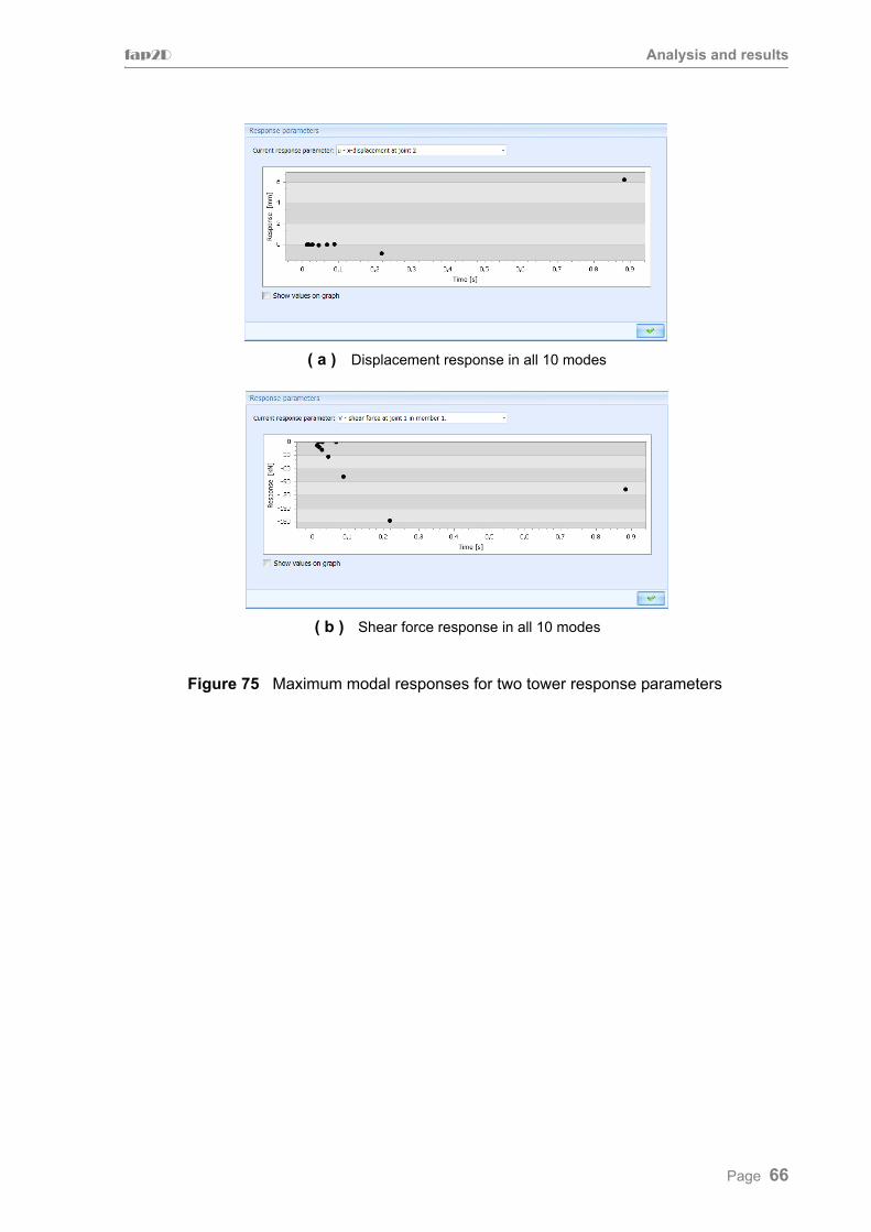
fap2D Analysis and results
( a ) Displacement response in all 10 modes
( b ) Shear force response in all 10 modes
Figure 75 Maximum modal responses for two tower response parameters
Page 66

fap2D Analysis and results
6.10 Steel design1
For structures with steel components, fap2d offers a capacity check, according to the rules and regulations of Eurocode 3, for all steel members with predefined or para-metric cross sections. This facility is available from the result view following a linear or nonlinear static analysis, or a forced dynamic analysis (including earthquakes).
Three different checks are available:- elastic stress control (1),- cross section control (2), and- component control (3).
1. The elastic capacity of a particular cross section is governed by initial yielding at the most stressed point of the section. The VON MISES yield criterion is used; hence yielding starts when the effective (VON MISES) stress σj is equal to the material yield strength fy , or rather the design strength fd . The code requirement is simply
(27)
In 2D the effective stress, in terms of axial stress σx and shear stress τ, is
(28)
At each node of steel members, the program calculates σj and the capacity or utili-zation index κ defined as
(29)
and presents the index as a color “map”. In order to satisfy the code κ should be smaller than or equal to 1 (one).
2. The cross section control is a fairly complex control which will not be dealt with in any detail here. In short the code defines 4 classes of cross sections, the purpose of which is to incorporate the effect of local buckling of the cross section itself on the section’s capacity, in such a way as to avoid this type of buckling. Controls are carried out for the section forces present, individually and in combination, according to the rules of the code.Sections of class 1 and 2 are checked for their plastic capacity, while sections of class 3 are subjected to an elastic control. It should be emphasized that currently the program does not handle sections of class 4.
3. The component control is applied to all straight steel beam members of constant cross section subject to compression. The in-plane buckling load is estimated through the results from a linearized buckling analysis carried out (automatically) by the program for the actual load combination. For each relevant member, the appropriate controls, considering the axial compression and the largest bending moment, are carried out, and the entire member is attributed this (highest) index.
1. It should be emphasized that this facility is not complete, nor is it thoroughly tested. At the end of this section you will find three tables indicating what is implemented and what is not implemented.
σj fd≤fy
γM0--------=
σj σx2 3τ2+=
κ σj fd⁄=
Page 67
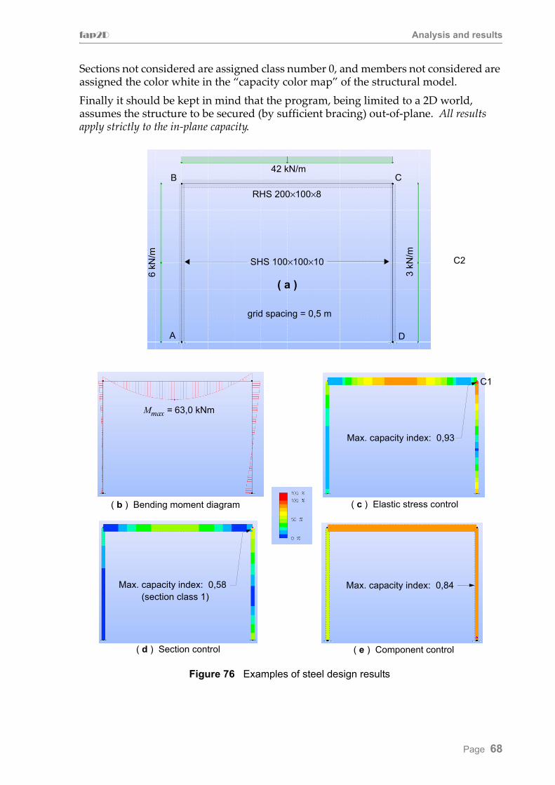
fap2D Analysis and results
Sections not considered are assigned class number 0, and members not considered are assigned the color white in the “capacity color map” of the structural model.Finally it should be kept in mind that the program, being limited to a 2D world, assumes the structure to be secured (by sufficient bracing) out-of-plane. All results apply strictly to the in-plane capacity.
C
SHS 100×100×10
RHS 200×100×8
grid spacing = 0,5 m
B
A D
42 kN/m
6 kN
/m
3 kN
/m
( c ) Elastic stress control
( d ) Section control ( e ) Component control
( b ) Bending moment diagram
( a )
Figure 76 Examples of steel design results
C2
Mmax = 63,0 kNm
Max. capacity index: 0,93
C1
Max. capacity index: 0,58(section class 1)
Max. capacity index: 0,84
Page 68

Typical results
Figure 76 shows some results from steel design checks applied to a simple steel frame following a linear static analysis. Right clicking the top of the right-hand column of figures 76c and d, produce the result boxes of figure 77a and b, respectively.
The section control formulas of Eurocode 3 have been developed for section forces obtained by linear static analysis, and the component control following a linear ana-lysis requires some estimate of the second order effects (e.g. buckling load).If a nonlinear analysis is carried out, the computed section forces already incorporate the higher order geometric effects. Hence, the only control available, following a non-linear analysis, is the elastic stress control. Figure 78b shows the capacity color map for the elastic stress control following a nonlinear analysis of the frame of figure 76a. The frame has, in addition to the loading of figure 76a, been subjected to a geometric imperfection, in the shape of the first buckling mode, shown in figure 78a.
On the following page, three tables will show the status of the steel design facility.
( a ) Elastic stress control ( b ) Section control
Figure 77 Detailed steel design results (apply to points C1 and C2 of figure 77)
( b ) Elastic stress control( a ) Geometric imperfection
Figure 78 Steel design based on nonlinear static analysis (with imperfection)
Max. capacity index: 0,96Max. amplitude: 12 mm
Page 69
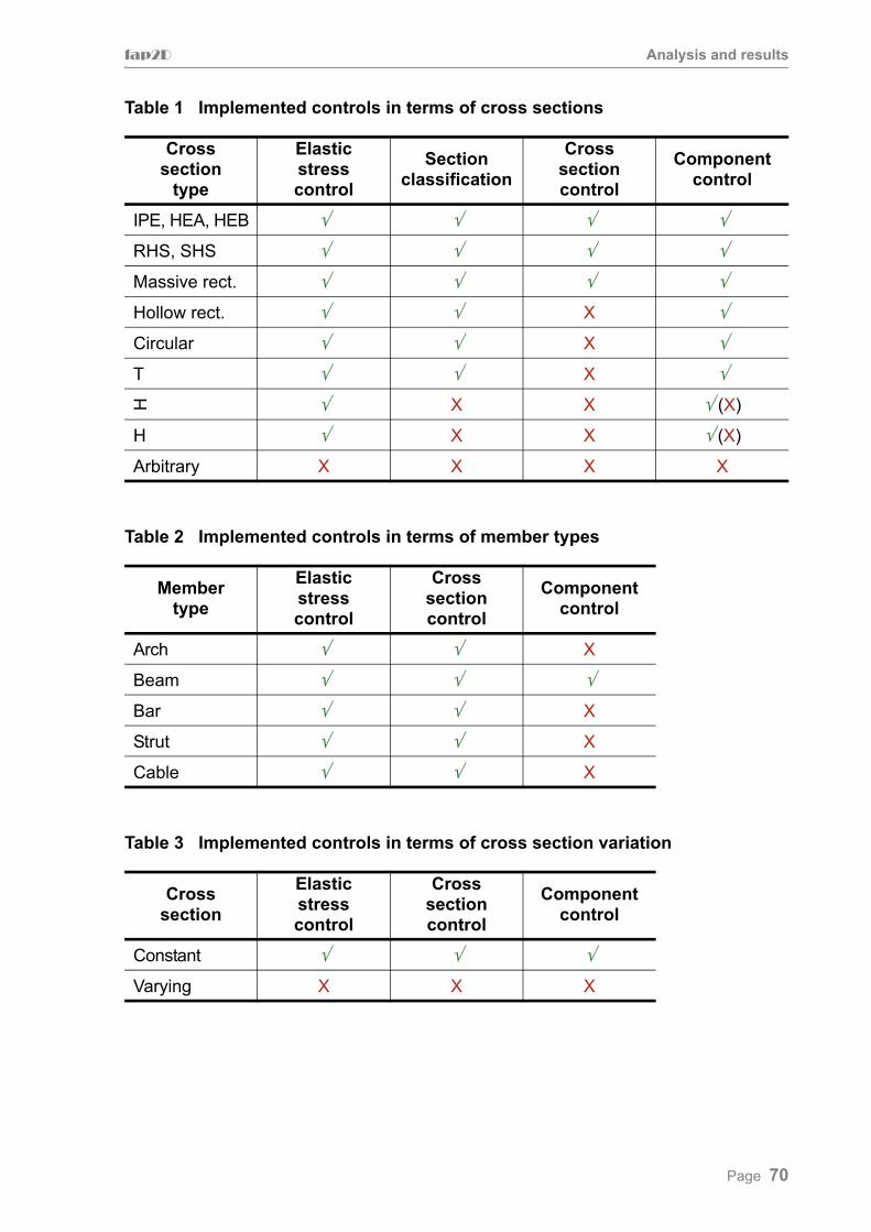
fap2D Analysis and results
Table 1 Implemented controls in terms of cross sections
Table 2 Implemented controls in terms of member types
Table 3 Implemented controls in terms of cross section variation
Crosssection
type
Elasticstresscontrol
Sectionclassification
Crosssectioncontrol
Componentcontrol
IPE, HEA, HEB √ √ √ √
RHS, SHS √ √ √ √
Massive rect. √ √ √ √
Hollow rect. √ √ X √
Circular √ √ X √
T √ √ X √
H √ X X √ (X)
H √ X X √ (X)
Arbitrary X X X X
Membertype
Elasticstresscontrol
Crosssectioncontrol
Componentcontrol
Arch √ √ X
Beam √ √ √
Bar √ √ X
Strut √ √ X
Cable √ √ X
Crosssection
Elasticstresscontrol
Crosssectioncontrol
Componentcontrol
Constant √ √ √
Varying X X X
Page 70
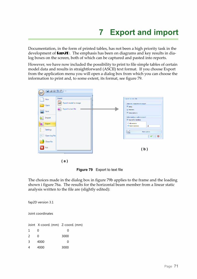
7 Export and import
Documentation, in the form of printed tables, has not been a high priority task in the development of fap2D. The emphasis has been on diagrams and key results in dia-log boxes on the screen, both of which can be captured and pasted into reports.However, we have now included the possibility to print to file simple tables of certain model data and results in straightforward (ASCII) text format. If you choose Export from the application menu you will open a dialog box from which you can choose the information to print and, to some extent, its format, see figure 79.
The choices made in the dialog box in figure 79b applies to the frame and the loading shown i figure 76a. The results for the horizontal beam member from a linear static analysis written to the file are (slightly edited):
fap2D version 3.1
Joint coordinates
Joint X-coord. (mm) Z-coord. (mm)
1 0 0
2 0 3000
3 4000 0
4 4000 3000
Figure 79 Export to text file
( b )
( a )
Page 71
fap2D Export and import
Member info.
Member Type Geometry Radius/height (mm) Joints Material Cross sect.
1 StraightBeam Straight 0 1, 2 Steel SHS 100x100x10
2 StraightBeam Straight 0 2, 4 Steel RHS 200x100x8
3 StraightBeam Straight 0 3, 4 Steel SHS 100x100x10
Cross section info.
Name Type A (mm^2) I (mm^4) ht (mm) hb (mm)
IPE 200 Predefined 2850 1,94E+07 100 100
RHS 200x100x8 Predefined 4450 2,2E+07 100 100
SHS 100x100x10 Predefined 3550 4,74E+06 50 50
Results for members (section forces).
Results for member 2
Member type: StraightBeam
Load combination: Default load combination
End joints: 2, 4
s (mm) = N (kN) V (kN) M (kNm)
0 -12,249 -79,1 14,688
80 -12,249 -75,74 8,3604
160 -12,249 -72,38 2,3012
240 -12,249 -69,02 -3,4892
320 -12,249 -65,66 -9,0107
400 -12,249 -62,3 -14,263
480 -12,249 -58,94 -19,247
560 -12,249 -55,58 -23,963
640 -12,249 -52,22 -28,409
720 -12,249 -48,86 -32,587
800 -12,249 -45,5 -36,495
880 -12,249 -42,14 -40,135
960 -12,249 -38,78 -43,506
1040 -12,249 -35,42 -46,609
1120 -12,249 -32,06 -49,442
1200 -12,249 -28,7 -52,007
1280 -12,249 -25,34 -54,303
1360 -12,249 -21,98 -56,33
Page 72

fap2D Export and import
1440 -12,249 -18,62 -58,089
1520 -12,249 -15,26 -59,578
1600 -12,249 -11,9 -60,799
1680 -12,249 -8,5396 -61,751
1760 -12,249 -5,1796 -62,434
1840 -12,249 -1,8196 -62,849
1920 -12,249 1,5404 -62,994
2000 -12,249 4,9004 -62,871
2080 -12,249 8,2604 -62,479
2160 -12,249 11,62 -61,818
2240 -12,249 14,98 -60,888
2320 -12,249 18,34 -59,69
2400 -12,249 21,7 -58,223
2480 -12,249 25,06 -56,487
2560 -12,249 28,42 -54,482
2640 -12,249 31,78 -52,208
2720 -12,249 35,14 -49,666
2800 -12,249 38,5 -46,855
2880 -12,249 41,86 -43,774
2960 -12,249 45,22 -40,426
3040 -12,249 48,58 -36,808
3120 -12,249 51,94 -32,922
3200 -12,249 55,3 -28,766
3280 -12,249 58,66 -24,342
3360 -12,249 62,02 -19,649
3440 -12,249 65,38 -14,688
3520 -12,249 68,74 -9,4574
3600 -12,249 72,1 -3,9582
3680 -12,249 75,46 1,8099
3760 -12,249 78,82 7,8467
3840 -12,249 82,18 14,152
3920 -12,249 85,54 20,727
4000 -12,249 85,54 27,57
The import function, see figure 79a, is limited to joint coordinates. The coordinates must be organized in a text file, in a format similar to that which the joint coordinates are printed by the export function, that is identifyer (joint number), x-coordinate and finally z-coordinate; one joint per line.
Page 73
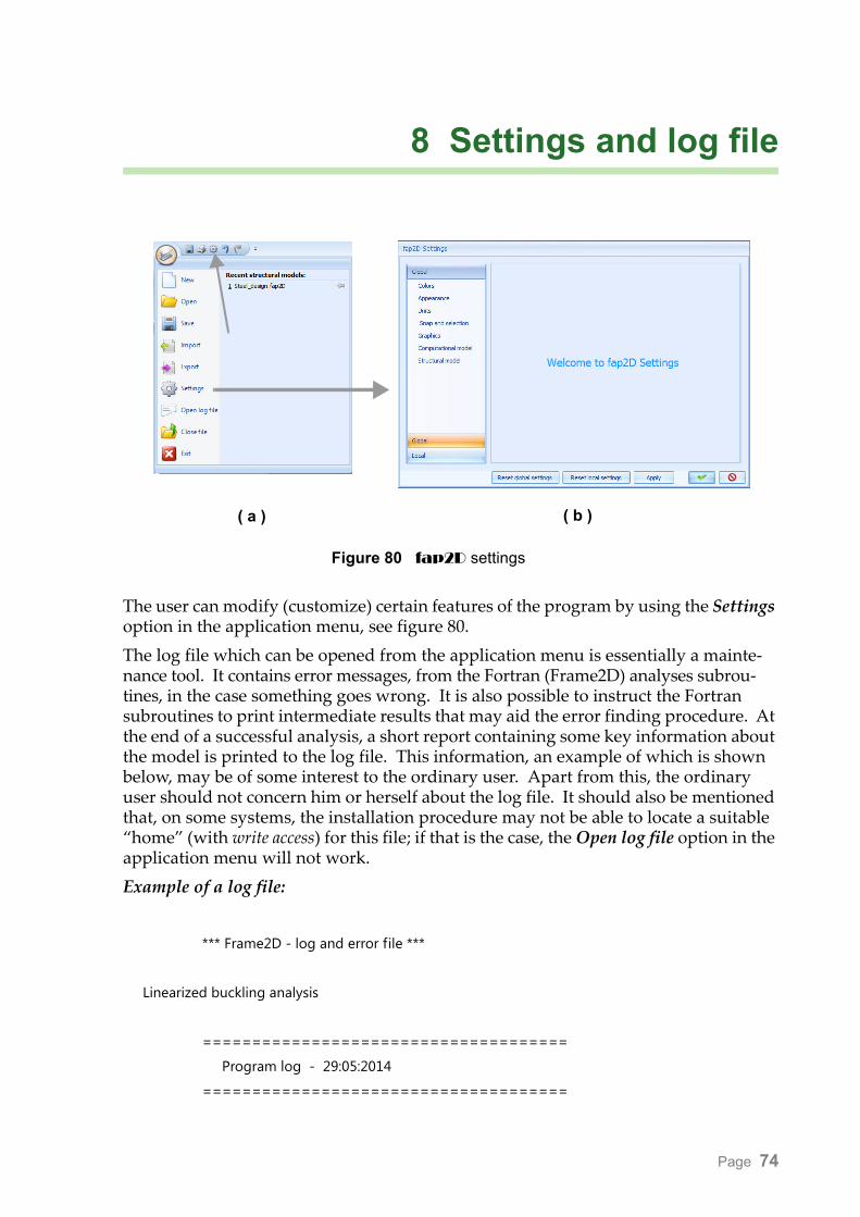
8 Settings and log file
The user can modify (customize) certain features of the program by using the Settings option in the application menu, see figure 80.The log file which can be opened from the application menu is essentially a mainte-nance tool. It contains error messages, from the Fortran (Frame2D) analyses subrou-tines, in the case something goes wrong. It is also possible to instruct the Fortran subroutines to print intermediate results that may aid the error finding procedure. At the end of a successful analysis, a short report containing some key information about the model is printed to the log file. This information, an example of which is shown below, may be of some interest to the ordinary user. Apart from this, the ordinary user should not concern him or herself about the log file. It should also be mentioned that, on some systems, the installation procedure may not be able to locate a suitable “home” (with write access) for this file; if that is the case, the Open log file option in the application menu will not work.Example of a log file:
*** Frame2D - log and error file ***
Linearized buckling analysis
=====================================
Program log - 29:05:2014
=====================================
Figure 80 fap2D settings
( b )( a )
Page 74
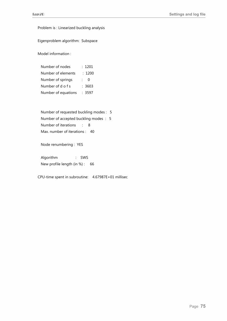
fap2D Settings and log file
Problem is : Linearized buckling analysis
Eigenproblem algorithm: Subspace
Model information :
Number of nodes : 1201
Number of elements : 1200
Number of springs : 0
Number of d o f s : 3603
Number of equations : 3597
Number of requested buckling modes : 5
Number of accepted buckling modes : 5
Number of iterations : 8
Max. number of iterations : 40
Node renumbering : YES
Algorithm : SWS
New profile length (in %) : 66
CPU-time spent in subroutine: 4.67987E+01 millisec
Page 75