
Whitepaper A Developers Guide to Accelerating Microsoft Excel Models With Platform Symphony
Upload
chabane-louizaCategory
view
136download
2
© Global Research & Analytics Dept.| First Year Anniversary
CH&Cie Global Research & Analytics is glad to present its
1st
Year
Anniversary


© Global Research & Analytics Dept.| First Year Anniversary
1
Introduction
By Benoit Genest, Head of the Global Research & Analytics Dept.
“Only one year after its creation, the GRA team has been completely transformed.
Surpassing all of the original ambitions, the team now stretches over three zones
(Europe, Asia and the US) and continues to grow.
Our philosophy is distinctly influenced by the gratification of working together on
subject matter which daily fascinates and inspires us. It also conveys the richness
of our exchanges, as we collaborate with several practitioners and enthusiasts.
This document has no other purpose than to bring some responsive elements to
the questions we face constantly, reminding us also to practice patience and
humility - for many answers are possible, and the path of discovery stretches out
long before us…”
Benoit Genest

Summary
Introduction
by Benoit Genest, Head of Global Research & Analytics Dept.
Optimization of Post-Scoring Classification and Impact
on Regulatory Capital for Low Default Portfolios by Ziad Fares
Value-at-Risk in turbulence time by Zhili Cao
Collateral optimization – Liquidity & Funding Value
Adjustments, Best Practices by David Rego & Helene Freon
CVA capital charge under Basel III standardized
approach by Benoit Genest & Ziad Fares
Basel II Risk Weight Functions by Benoit Genest & Leonard Brie
2
3
4
5
6
1

© Global Research & Analytics Dept.| First Year Anniversary
Optimization of Post-Scoring Classification
and Impact on Regulatory Capital for Low
Default Portfolios
By Ziad Fares
Validated by Benoit Genest
April, 2014

© Global Research & Analytics Dept.| First Year Anniversary
4
Table of contents
Abstract ................................................................................................................................................... 5
1. Introduction ..................................................................................................................................... 6
2. The main credit risk measurement methods .................................................................................... 7
2.1. Heuristic models ...................................................................................................................... 7
2.1.1. Classic rating questionnaires ........................................................................................... 7
2.1.2. Fuzzy logic systems ......................................................................................................... 7
2.1.3. Expert systems ................................................................................................................. 7
2.1.4. Qualitative systems .......................................................................................................... 8
2.2. Statistical models ..................................................................................................................... 8
2.2.1. Market Theory ................................................................................................................. 8
2.2.2. Credit Theory .................................................................................................................. 8
3. The Theory and the Methodology behind classification trees ......................................................... 8
3.1. The use of classification techniques in credit scoring models ................................................. 8
3.2. Principle of the decision trees and classic classifications...................................................... 10
3.3. Methodological basis of classification trees .......................................................................... 12
3.3.1. Classification and Regression Tree (CART) ................................................................. 12
3.3.2. CHi-squared Automation Interaction Detection (CHAID) ........................................... 13
3.3.3. Quick Unbiased Efficient Statistical Tree (QUEST) ..................................................... 15
3.3.4. Belson criteria ................................................................................................................ 16
3.4. Conditions and constraints to optimize the segmentation ..................................................... 17
4. Building a rating scale on a Low Default Portfolio and the impacts on the regulatory capital ..... 18
4.1. Framework of the study ......................................................................................................... 18
4.1.1. Purpose of the analysis .................................................................................................. 18
4.1.2. What are the dimensions involved in the study? ........................................................... 19
4.1.3. Description of the portfolio on which the study was conducted ................................... 19
4.2. Presentation of the results ...................................................................................................... 20
4.2.1. Building the rating scale on the modeling sample ......................................................... 20
4.2.2. Verifying the stability of the rating scale ...................................................................... 23
4.2.3. Establishing a relationship between the number of classes and the impact on regulatory
capital ....................................................................................................................................... 25
Conclusion ............................................................................................................................................. 27
Bibliography .......................................................................................................................................... 28

Optimization of Post-Scoring Classification and Impact on Regulatory Capital for Low Default Portfolios
5
Optimization of Post-Scoring Classification and
Impact on Regulatory Capital for Low Default
Portfolios
Abstract
After the crisis of 2008, new regulatory requirements have emerged with supervisors strengthening their position in terms of requirements to meet IRBA standards. Low Default Portfolios (LDP) present specific characteristics that raise challenges for banks when building and implementing credit risk models. In this context, where banks are looking to improve their Return On Equity and supervisors are strengthening their positions, this paper aims to provide clues for optimizing Post-Scoring classification as well as analyzing the relationship between the number of classes in a rating scale and the impact on regulatory capital for LDPs.
Key words: Basel II, Return On Equity, RWA, Classification trees, Rating scale, Gini, LDP

© Global Research & Analytics Dept.| First Year Anniversary
6
1. Introduction
The 2008 crisis was the main cause of tough market regulation and banks’ consolidation basement. These new constraints have caused a major increase in banks’ capital. As a result, banks need to optimize their return on equity, which has suffered a big drop (due both to a drop in profitability as well as an increase in capital).
Moreover, as this crisis showed loopholes in risk measurement and management, regulators’ tolerance becomes more and more stringent. Consequently, banks are facing challenges while dealing with Low Default Portfolios (LDP) and discerning the way to meet regulatory requirements in terms of credit risk management under the Advanced Approach (IRBA) of Basel rules.
The purpose of this paper is to focus on post-scoring classification for LDPs with the aim to study the possibility of building a rating scale for these portfolios, that meets regulatory requirements as well as to identify the opportunities to optimize RWA. This will be accomplished by studying the relationship between the number of classes within a rating scale and the impact on RWA. The analysis will follow different steps.
First, the different classification techniques will be detailed and studied from a theoretical point of view, leading to a clear understanding of the underlying statistical indicators and algorithms behind each technique. Moreover, the differences between the various techniques will also be made clear.
Second, once the classification techniques are analyzed, we will be placed from a credit scoring perspective and define the constraints that must be respected by the rating scale in order to be compliant with the regulatory requirements.
Third, a study will be conducted on a real Retail portfolio comprised of mortgage loans with a low frequency of loss events. The significant number of loans renders the granularity assumption reliable. The aim of the study is to build multiple rating scales using the different techniques, analyze the difference between the various ratings produced, and use this analysis to identify which classification technique provides the best results in terms of stability, discrimination and robustness for LDPs. Finally, the relationship between the number of risk classes and the impact on RWA will be established in order to identify potential opportunities for RWA optimization for LDPs.

Optimization of Post-Scoring Classification and Impact on Regulatory Capital for Low Default Portfolios
7
2. The main credit risk measurement methods
In order to provide the reader with a global view of the framework of this study, we will briefly overview the main credit measurement methods. These methods are a prerequisite for understanding the context in which this paper has been written.
2.1. Heuristic models
The “Heuristic” branch corresponds to all kinds of rather “qualitative” methods. These heuristic models are based on acquired experience. This experience is made of observations, conjectures or business theories. In the peculiar field of credit assessment, heuristic models represent the use of experience acquired in the lending business to deduce the future creditworthiness of borrowers. They subjectively determine the factors relevant to this creditworthiness as well as their respective weights in the analysis. It is important to note, however, that the adopted factors and weights are not validated statistically. Four main different types of heuristic models are presented here.
2.1.1. Classic rating questionnaires
Based on credit experts' experience, they are designed in the form of clear questions regarding factors that are determined to be of influence for creditworthiness assessment. To each type of answer are attributed an amount of points: for instance, as an answer to a “Yes/No” question, “Yes” means 1 point and “No” means 0. The number of points reflects the experts' opinion on the influence of the factors, but there is no place for subjectivity in the answer. The answers are filled in by the relevant customer service representative or clerk at the bank, and the points for all answers are added to obtain an overall score. The questions are usually about the customer's sex, age, marital status, income, profession, etc. These factors are considered to be among the most relevant ones for retail business.
2.1.2. Fuzzy logic systems
These systems, sometimes considered part of the expert systems, are a new area of research. The introduction of so-called “fuzzy” logic allows for the replacement of simple dichotomous variables (“high/low”) by gradated ones. For instance, when it comes to evaluating a return, a classical rule would be that the return is low under 15% and high above 15%. But that would mean that a 14.99% return would be “low” whereas 15% is “high”, which is absurd. The “fuzzification” process introduces continuity where it did not exist.
For instance, a return of 10% would be rated 50% “low”, 50% “medium” and 0% high, whereas in the first model it would have been rated simply “low”. Thus it determines the degree to which the low/medium/high terms apply to a given level of return. After this, the determined values undergo transforming processes according to rules defined by the expert system, and they are aggregated with other “fuzzified” variables or simple ones. The result is a clear output value, representing the creditworthiness of the counterpart. It must be noted that an inference engine being fed with fuzzy inputs will produce fuzzy outputs which must be “defuzzified” in order to obtain the final, clear output (e.g. a credit rating).
2.1.3. Expert systems
These are software solutions aiming to recreate human reasoning methods within a specific area. Just as a human brain would do, they try to solve complex and poorly structured problems and to make reliable conclusions. Consequently, expert systems belong to the “artificial intelligence” field. They are made of 2 parts: a knowledge base, with all the knowledge acquired

© Global Research & Analytics Dept.| First Year Anniversary
8
for the specific area, and an inference engine, which often uses “fuzzy” inference techniques and “if/then” production rules to recreate the human way of thinking.
2.1.4. Qualitative systems
Qualitative systems require credit experts to assign a grade for each factor which, overall, determines a global rating regarding one person’s credit. Technically speaking, this solution is used for corporate businesses.
2.2. Statistical models
These statistical models derive from two main theories that give birth to two sets of calculation methods.
2.2.1. Market Theory
Models derived from the so-called Market Theory are based on classical market finance models. The Merton model – the most famous of all Market Theory models - is based on the theory of financial asset evolution as formulated by Black, Scholes and Merton in the early 70's. Sometimes also called “Casual”, Market Theory models focus on a single explanation of default: what is the process that leads a firm to default? The Merton model, for instance, defines default as the moment that the firm's asset value falls below its debt value.
2.2.2. Credit Theory
Models derived from Credit Theory differ from Market Theory in that they do not focus on a single cause of default. Instead, they use statistical tools to identify the most significant factors in default prediction, which may vary from firm to firm. There are three different types of Credit Theory statistical models, outlined below. Regression and Multivariate Discriminant Analysis (MDA) is based on the analysis of the variables (for instance financial statements) that are the most discriminant between solvent and insolvent counterparts. Neural Networks, a fairly new model, attempts to reproduce the processing mechanisms of a human brain. A brain is made of neurons which are connected to one another by synapses. Each neuron receives information through synapses, processes it, then passes information on through other neurons, allowing information to be distributed to all neurons and processed in parallel across the whole network. Artificial neural networks also attempt to reproduce the human brain ability to learn. Bayesian models operate in real time, which means they are updated when the information is processed. As a result, Bayesian models help the credit score refreshes in the portfolio instantly. Furthermore, Bayesian systems use a technology of time-varying parameters that add a dynamic notion to the analysis. For instance, these models can use methods such as Markov Chain Monte Carlo that are very effective for conjunction. These models have proven to offer highly accurate estimations and predictions.
3. The Theory and the Methodology behind classification trees
3.1. The use of classification techniques in credit scoring models

Optimization of Post-Scoring Classification and Impact on Regulatory Capital for Low Default Portfolios
9
When building a credit scoring model - particularly when modeling the Probability of Default (PD) of counterparties (for instance for a retail portfolio) - the dependent variable (Y) is binary and can take two possible values:
� = ��� .� �ℎ ����� ������ �� � ��� � ���� ��ℎ� �ℎ ������� � ���� �ℎ ����� ������ � ����� ��ℎ� �ℎ ������� � ��. ��
�
Generally, the PD is modeled by using a logistic regression where a score is attributed to each counterparty based on explanatory variables that were accurately chosen (based on a statistical study showing their ability to predict the default of a counterparty) when building the model:
���� = ln ! "#� = 1 |&)1 − "#� = 1 |&) ) = ∝++ - ∝. #/). 0.#/)1.23
With:
- αi the parameters of the regression; - xi the explanatory covariates; - X = {xi}i=1..n - P(Y=1|X) is the conditional probability that Y = 1 (default of a counterparty) knowing
a given combination of the explanatory variables; - j reflects the modality of the explanatory variables (for qualitative variables as well as
discretized variables). The conditional probability can then be written as:
"#� = 1|&) = 11 + 456789 = 11 + 4#∝:; ∑ ∝=#>).?=#>)@=AB ) A score is then attributed to each counterparty. Given that the portfolio is constituted of many counterparties (for retail portfolios for instance), the abundance of score values may render the risks more difficult to manage. In other words, it is essential to regroup the individuals of the portfolio in clusters or classes to better reflect risk categories and make it more convenient for operational use. There are many techniques used to classify the individuals and build clusters such as:
- Neural Networks; - Bayesian Networks; - Kernel estimation (k-nearest neighbors); - Decision trees; - Classic classification.
This article is dedicated to classification techniques that are frequently used in the banking sector and more precisely in the credit scoring process. Consequently, a focus will be made on Decision trees and classic classification techniques. More precisely, it is the impact of the portfolio classification on RWA (and by extension on capital) that will be analyzed with the following two main axes:
- The nature of the classification technique;

© Global Research & Analytics Dept.| First Year Anniversary
10
- The number of classes created.
3.2. Principle of the decision trees and classic classifications
The decision tree technique is one of the most popular methods in credit scoring models. In fact it provides explicit rules for classification as well as presents features that are easy to understand. There are two types of decision trees: classification trees and regression trees. Consequently, decision trees are on the boundary between predictive and descriptive methods. For the purpose of this article only classification trees are considered since the prediction of the dependent variable has already been modeled using a logistic regression procedure. The principle of decision trees is to classify the individuals of a population based on a dividing (or discriminating) criterion. Based on this criterion, the portfolio is divided into sub-populations, called nodes. The same operation is repeated on the new nodes until no further separation is possible. Consequently, decision trees are an iterative process since the classification is built by repeating the same operation several times. Generally, a parent node is separated into two child nodes:
Furthermore, there are three main steps in creating decision trees:
- First Step | Initialization: the first step aims to define which variable will serve as a dividing criterion and which variable(s) will be used to build and define the clusters or the classes. For instance, in the credit scoring process, the dividing variable is the default variable and the variable used to build the classes is the score. In fact, the aim is to build classes that reflect different levels of credit risk, or in other words, different values of default rate. Consequently, the separation will be built in order to isolate individuals with the same credit risk level into classes. Thus, the score values will be grouped into classes where the default rate in each class is significantly different. Moreover, the purpose of the credit scoring model is to predict the default probability of a performing loan therefore a score value will be attributed to this loan which will allow it to be assigned to a risk category (or class). Finally, during this step, the nature of the tree is defined (CART, CHAID, etc…) and its depth (or the potential maximum number of classes) is fixed;
- Second Step | Distribution of the population in each node: After initializing the tree, the separation process is launched. The purpose is to obtain classes with significantly

Optimization of Post-Scoring Classification and Impact on Regulatory Capital for Low Default Portfolios
11
different distribution. This process is repeated until no further separation is possible. The stop criterion of the process depends on the tree used, but in general it is related to the purity of the tree, the maximum numbers of nodes, the minimum number of individuals in a node, etc…:
- Third Step | Pruning: Pruning is essential when the tree is too deep considering the size of the portfolio. This might lead to classes with low number of individuals which will introduce instability in the classification as well as a random component for these classes. Moreover, if the tree is too deep, the risks of overfitting are high. In other words, the classification on the training (or modeling) sample might provide good results but the error rate might be too high when this classification is used on the application sample:
Concerning classic classification techniques, the paper focuses mainly on two types:
- Create classes with the same number of individuals: this first technique allows the creation of classes with the same number of individuals by class. For instance, when

© Global Research & Analytics Dept.| First Year Anniversary
12
applied on a credit portfolio, the score values are classified in the descending order. Then, knowing the number of classes, a classification is built by regrouping the same number of (ordered) individuals;
- Create classes with the same length: this second technique allows the creation of classes with the same length or in other words with the same intervals. For instance, when applied on a credit portfolio, the score values are also classified in the descending order. Then, individuals are grouped into classes with the same length.
These techniques are simple in terms of application as they are not based on statistical indicators. Consequently, there is no limitation in terms of number of classes.
3.3. Methodological basis of classification trees
Classification trees are mainly based on a statistical approach. The methodology used differs from one tree to another. More precisely, it is the splitting criterion (or in other words the statistical indicator used to assess the level of differentiation between two classes) that differs. The purpose of this paragraph is to explain for each type of tree the nature of the splitting criterion used and its methodological basis.
3.3.1. Classification and Regression Tree (CART)
The CART tree was invented in 1984 by L.Breiman, R.A Olshen, C.J Stone and J.H Friedman. It is one of the most used decision trees and is renowned for its effectiveness and performance. The main characteristics of this tree are various, which makes it applicable in every circumstance:
- It can be used on all kinds of variables (qualitative, quantitative, …);
- It can also be used for continuous variables (infinite number of categories) or discrete variables (finite number of categories);
- It has a pruning algorithm that is more elaborated that the CHAID technique. In fact, the CART builds a tree with the maximum number of nodes. Then, the algorithm compares the purity (by comparing the error rate) of sub-trees using a sequence of pruning operations and selects the one which maximizes the purity of a tree;
- Finally, one key element in the performance of this technique is its ability to test all possible splits and then to select the optimal one (using the pruning algorithm).
Even though this technique is reliable it has some drawbacks:
- It is binary (one parent node gives two or less child nodes) which might provide trees that are too deep and somehow complex in terms of interpretation;
- The processing time might be long. In fact, this can happen when applied for credit risk purposes, where there are too many values of score (knowing that a retail portfolio with high granularity is considered).
The splitting criterion used in the CART is the Gini index. This index measures the population diversity or, in another words, the purity of a node. The Gini index of a node is measured as follows:

Optimization of Post-Scoring Classification and Impact on Regulatory Capital for Low Default Portfolios
13
C�17D9 = 1 − - ".E = - - ". . ">F
>23,>H.
F.23
F.23
Because,
I- ".F
.23JE = 1 = - ".E + - - ". . ">
F>23,>H.
F.23
F.23
Where,
- Gininode is the Gini index of a node; - m is the number of categories of the dependent variable; - Pi is the relative frequency of the ith category of the dependent variable.
If the Gini index increases, the purity of the node decreases. Consequently, during the separation phase, the best split is the one that provides the best decrease in the Gini index. In other words, the criterion to be minimized is:
C�59KL8LM.71 = - �N� . C�N = 8N23
-OPQ�N� . - - ".#R). ">#R)F
>23,>H.
F.23 S
TU8
N23
Where, - r is the optimal number of child nodes that minimizes the Giniseperation index; - nk is the number of individuals in the child node k; - n is the total number of individuals in the parent node :
� = - �N8
N23
Finally, it is also possible to use another splitting criterion. Using the same mechanism, the entropy reduction process could also lead to good results. The splitting criterion is:
V������17D9 = - ". . log #".)F.23
3.3.2. CHi-squared Automation Interaction Detection (CHAID)
This technique was developed in South Africa in 1980 by Gordon V. Kass.
The main characteristics of this tree are:
- It is mainly used for discrete and qualitative dependent and independent variables;
- It can be used for both classification and prediction;
- It can be interpreted easily and it is non-parametric. In other words, it does not rely on the normality distribution of data used;
© Global Research & Analytics Dept.| First Year Anniversary
14
- CHAID is not a binary tree which provides wider trees rather than deeper.
Yet, this technique also presents some drawbacks:
- This technique uses the X2 (Chi-squared index) as a splitting criterion. Consequently, this test requires a significance threshold in order to work accurately. Somehow, this threshold is a parameter to be defined and its level is often arbitrary and depends on the size of the sample;
- It requires large samples and might provide unreliable results when applied on small samples.
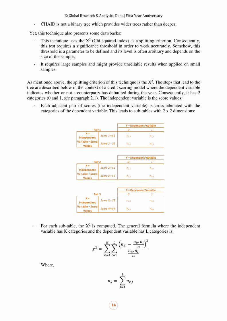
As mentioned above, the splitting criterion of this technique is the X2. The steps that lead to the tree are described below in the context of a credit scoring model where the dependent variable indicates whether or not a counterparty has defaulted during the year. Consequently, it has 2 categories (0 and 1, see paragraph 2.1). The independent variable is the score values:
- Each adjacent pair of scores (the independent variable) is cross-tabulated with the categories of the dependent variable. This leads to sub-tables with 2 x 2 dimensions:
- For each sub-table, the X2 is computed. The general formula where the independent
variable has K categories and the dependent variable has L categories is:
YE = - - Z�N[ − �N. �[� \E�N. �[�
][23
^N23
Where,
�N = - �N,[]
[23
0 1
Score 1 = S1 n1,0 n1,1
Score 2 = S2 n2,0 n2,1
0 1
Score 2 = S2 n2,0 n2,1
Score 3 = S3 n3,0 n3,1
0 1
Score 3 = S3 n3,0 n3,1
Score 4 = S4 n4,0 n4,1
Y = Dependent Variable
X =
Independent
Variable = Score
Values
Pair 3
Y = Dependent Variable
X =
Independent
Variable = Score
Values
Y = Dependent Variable
X =
Independent
Variable = Score
Values
Pair 1
Pair 2

Optimization of Post-Scoring Classification and Impact on Regulatory Capital for Low Default Portfolios
15
�[ = - �N,[^
N23
� = �N + �[
- For each sub-table, the p-value associated to the X2 is computed. If the p-value is superior to the merging threshold (in general this threshold is set to 0.05), then the two categories are merged since this means that these categories differ the least on the response. This step is repeated until all pairs have a significant X2. If the X2 is significant, the categories could be split into child nodes. Moreover, if the minimum number of individuals is not respected in a node, it is merged with an adjacent node;
- Finally, the Bonferroni correction could be used to prevent the over-evaluation of the significance of multiple-category variables.
3.3.3. Quick Unbiased Efficient Statistical Tree (QUEST)
This technique was invented in 1997 by Loh and Shih. The main characteristics of this tree are:
- It can be used for all kinds of variables (continuous, discrete, ordinal and nominal variables);
- The algorithm yields to a binary tree with binary splits;
- It has the advantage of being unbiased in addition to having a high speed computational algorithm.
The steps of the technique are presented below in the context of a credit scoring model:
- First, as mentioned above, the independent variable is well known. Consequently, the description of the entire Quest algorithm is unnecessary since the Anova F-test as well as Levene’s F-test (and Pearson’s X2) have been used to select which independent variables are best suited in explaining the dependent variable. Knowing that in the credit scoring model only one independent variable is used, this part of the algorithm might be skipped;
- Second, the Split criterion is based upon the Quadratic Discriminant Analysis (QDA) instead of the Linear Discriminant Analysis for the FACT algorithm. The process used is as follows:
o In credit scoring models, the final tree is generally constituted of multiple classes (in general from 5 to 10 classes). Consequently, knowing that more than two classes are required, the first split is based on separating the portfolio into two super-classes. The two-mean clustering method is used to do so. The purpose is to create two classes where the means are the most distant. Consider that the sample is constituted of n observations. These observations are grouped into 2 classes by optimizing the Euclidean distance to the mean of each class:
min - - |0> − a.|E
?b ∈ d=
E
.23

© Global Research & Analytics Dept.| First Year Anniversary
16
Where xj are the observations in the class Ci and mi the mean of the class Ci
o Then a QDA is performed on these two super-classes in order to the find optimal splitting point. The QDA makes the assumption that the population in the two classes is normally distributed. Consequently, the normal densities are considered and the split point is determined as the intersection between the two Gaussian curves. Consequently, the equation to be resolved is :
#0, a3, e3) = 1√2h. e3 . 4#?4FB)iE.jB = #0, aE, eE) = 1√2h. eE . 4#?4Fi)iE.ji
Where m is the mean and σ the standard deviation of the class (1 or 2).
By applying the logarithm function on the equation we obtain:
log k 1√2h. e3 . 4#?4FB)iE.jB l = ��� k 1√2h. e3l − #0 − a3)E2. e3 = ��� k 1√2h. eEl − #0 − aE)E
2. eE
−���#e3) − 12. e3 #0E + a3E − 20a3) = −���#eE) − 12. eE #0E + aEE − 20aE)
Finally, the quadratic equation becomes:
m 12. eE − 12. e3n 0E + ma3e3 − aEeE n 0 + I aEE2. eE − a3E2. e3 + ��� meEe3nJ = 0
o This step is repeated until the maximal tree length is obtained and the pruning algorithm is activated to optimize the tree.
3.3.4. Belson criteria
The characteristics of the Belson criteria technique are:
- It is used to optimize the discretization by building classes that optimize the correlation between the dependent and the independent variable;
- It does not yield to a binary tree;
- It might provide trees that are wide;
- No thresholds (for splitting or merging) are necessary for this technique.
The steps that lead to the segmentation are:
- This algorithm is very similar to the CHAID algorithm in terms of process and steps of segmentation. What really changes is the splitting criterion;

Optimization of Post-Scoring Classification and Impact on Regulatory Capital for Low Default Portfolios
17
- In fact, the Belson criterion is a simplified version of the X2 test and it is very useful when the variables are dichotomous which is the case for credit scoring models where the dependent variable is dichotomous. The steps leading to the segmentation contain a contingency table with 2 x 2 dimension making the independent variable dichotomous at each iterative calculus;
- More precisely, the algorithm is:
The Belson criterion is computed for each pair:
p��q = r�3,+ − s3� �3r = r�E,+ − sE� �3r = r�3,3 − s3� �Er = r�E,3 − sE� �Er Where,
s3 = �3,+ + �3,3
sE = �E,+ + �E,3
�3 = �3,+ + �E,+
�E = �3,3 + �E,3
� = �3 + �E = s3 + sE
The splitting point is the one that maximizes the Belson Criterion.
3.4. Conditions and constraints to optimize the segmentation
In a credit scoring model, while building the risk classes, there are some conditions and constraints that must be fulfilled in order to have a robust model that will allow measuring accurately the risks within the portfolio.
In fact, regulators and central banks pay a lot of attention to the way risk classes have been constructed. Moreover, for each risk manager having a rating scale that provides accurate results is a must-have since it will allow him or her to fully understand the structure of the portfolio as well as act as a catalyst to take actions if the risk limits are not respected.
The conditions and constraints that must be taken into account are:
- Number of individuals in each class:
o First, it is important that the number of individuals in each class does not exceed a certain limit since it will show that the discrimination power of the rating scale is not sufficient enough. In general, the size of a class must not exceed 40% of the total portfolio;
o Second, the minimum number of individuals within a class must not be too low. In fact, this might introduce instability in the rating scale since a little change in
0 1 ∑
Score 1 = S1 n1,0 n1,1 b1
Score 2 = S2 n2,0 n2,1 b2
∑ n1 n2 n
Y = Dependent Variable
X =
Independent
Variable = Score
Values
Pair 1

© Global Research & Analytics Dept.| First Year Anniversary
18
the population might have a significant impact on the default rate. Moreover, a class with few individuals might not be sufficiently consolidated or not sufficiently representative of a homogenous risk class. In general, each class must at least have more than 100 counterparts.
- Homogeneity within a class / heterogeneity between classes:
o First, the aim of the rating scale is to build classes that are homogenous in terms of risk profile. Consequently, the intra-class dispersion must be low in order to ensure that the individuals that are grouped into a risk class share the same characteristics as well as the same risk profile. If this dispersion is high, a recalibration is needed;
o Second, the level of risk must be different from a class to another. In fact, the rating scale purpose is to build clusters where each cluster represents a different level of risk. Consequently, the dispersion between classes must be high showing that these classes are differentiated in terms of risk profile.
- Stability of the classes: o First, the classes must guarantee a stability of the population across time (or a
giving horizon). This is very important since it will affect the predictive power of the model. Consequently, indicators such as the Population Stability Index (PSI) must be performed and monitored across time ;
o Second, the rating scale must also ensure that the default rate within a class is stable across time which means that the risk profile within a class is stable allowing the model to have a good predictive power;
o Third, the stability (as well as the discrimination power) could also be appreciated by making sure that the default rates series between classes do not cross each other. This means that there are no inversions between classes making the model stable over time.
- Discrimination and progressiveness of the default rate: o The levels of default rates from one class to another must be progressive. This
means that the function that represents the default rate by risk class is a monotonously increasing function;
o This guarantees that there are no inversions between classes.
In the following part, a rating scale is built for a Retail Low Default Portfolio (LDP) using the different techniques mentioned above. When building the rating scales, the conditions and constraints mentioned above have a significant meaning since we are dealing with a LDP.
4. Building a rating scale on a Low Default Portfolio and the impacts on
the regulatory capital
4.1. Framework of the study
4.1.1. Purpose of the analysis
The analysis presented in this section regards the building of an efficient rating scale for a Low Default Portfolio and analyzing the relationship between the number of classes and the impact on regulatory capital.

Optimization of Post-Scoring Classification and Impact on Regulatory Capital for Low Default Portfolios
19
In fact, a LDP has specific characteristics that present challenges for risk quantification. Given the low frequency of loss events, applying a statistical treatment to build a score and a rating scale might not be an easy task. Consequently, the industry participants expressed concerns regarding LDPs since their structure could lead to unstable models which could imply that these LDPs do not meet the regulatory requirements and standards and therefore excluding them from the IRB perimeter. The purpose of this part is to show that it is possible to build a stable rating scale that respects the conditions and constraints mentioned in paragraph 2.4 by applying a statistical treatment. Then, the optimization of RWA is also analyzed. More specifically, for a LDP, does the number of classes have a significant impact on the regulatory capital? Furthermore, is it possible to efficiently optimize the RWA by adjusting the number of classes?
4.1.2. What are the dimensions involved in the study?
There are three dimensions that are taken into account for the study: The first dimension concerns the nature of the classification technique used to build the rating scale. In fact, all types of techniques mentioned above in this article are performed. The purpose is to understand how the results differ from one technique to another and where the difference arises. Another purpose is to test which technique is best suited for LDP by providing accurate and stable results in line with the regulatory standards and risk management. The second dimension concerns the number of classes. In fact, for each segmentation technique, different simulations are realized by taking the number of classes as an input. More precisely, the number of classes is varied until the maximum size of the tree is reached. Then the relationship between the number of classes and the impact on RWA (and thus, on regulatory capital) is studied. Another purpose is to understand the performance of the different techniques while changing the number of classes and thus the depth of the tree. The third dimension is time. The purpose here is to make sure that the rating scale built is stable over time and thus that its predictive power is good. Moreover, comparing the different techniques and their behavior over time allows a better understanding of the compatibility between the underlying algorithm of each technique and the characteristics of a LDP. By mixing these three dimensions, the study will provide answers and solutions to the concerns raised by market participants towards the treatment of LDP and its compliance with IRB requirements.
4.1.3. Description of the portfolio on which the study was conducted
As mentioned above, the portfolio on which the study was conducted is a Mortgage portfolio. This portfolio is characterized by a low frequency of loss events. The modeling window is the date 08312009 which means that all performing loans at 08312009 are considered. These loans are analyzed from 09012009 to 08312010 by trying to identify which counterparts defaulted. Consequently it is the one year default rate that is modeled. For the purpose of the study, the score has already been constructed, based on the best practices in the industry. The score shows good performances even though the portfolio considered is a

© Global Research & Analytics Dept.| First Year Anniversary
20
LDP. The methodology used to build the score is not the core subject of the study. In fact, the focus is on the rating scale and therefore the methodology of the score won’t be detailed here. The distribution of the number of counterparts in the portfolio is:
The one-year default rate at 08312009 is 0.55%. The number of counterparties is acceptable making the portfolio sufficiently granular. The evolution of the default rate on different time windows is:
The default rate series presents a slight tendency to decrease.
4.2. Presentation of the results
4.2.1. Building the rating scale on the modeling sample
The first step of the study is to build the rating scale on the modeling sample. As mentioned above, the modeling window is 08312009. The different techniques have been performed on this sample by changing the depth of the tree and the number of classes. The different results are summarized in the following matrix:

Optimization of Post-Scoring Classification and Impact on Regulatory Capital for Low Default Portfolios
21
The first finding concerns the variety of results obtained. In fact, the rating scale and the clustering might differ significantly from one technique to another. More precisely, it is easy to observe that the distribution of the default rate differs on the technique used. This is also true
Nb of classes QUEST CHAID CART BELSON ISO interval ISO distrib.
1 0,4% 0,4% 0,0% 0,1% 0,3% 0,0%
2 20,8% 33,7% 1,0% 3,0% 12,2% 1,0%
1 0,3% 0,0% 0,1% 0,2% 0,0%
2 6,0% 0,3% 1,1% 3,1% 0,1%
3 33,7% 2,9% 9,2% 33,3% 1,5%
1 0,1% 0,0% 0,1% 0,1% 0,0%
2 1,6% 0,3% 1,1% 1,2% 0,1%
3 16,9% 1,1% 5,6% 9,2% 0,2%
4 65,5% 8,7% 22,0% 47,6% 1,9%
1 0,0% 0,1% 0,1% 0,1% 0,0%
2 0,2% 1,1% 0,4% 0,5% 0,1%
3 0,7% 5,0% 1,1% 4,8% 0,1%
4 4,3% 8,4% 5,6% 19,7% 0,3%
5 20,8% 33,7% 22,0% 64,3% 2,2%
1 0,0% 0,0% 0,0% 0,0% 0,0%
2 0,2% 0,3% 0,3% 0,3% 0,0%
3 0,7% 1,1% 1,1% 2,2% 0,1%
4 4,3% 5,0% 5,0% 7,6% 0,1%
5 16,9% 8,4% 8,4% 26,0% 0,4%
6 64,3% 33,7% 33,7% 66,0% 2,6%
1 0,0% 0,0% 0,0% 0,0%
2 0,3% 0,3% 0,2% 0,0%
3 1,1% 1,1% 1,1% 0,1%
4 5,0% 5,0% 5,6% 0,1%
5 8,4% 8,4% 12,2% 0,3%
6 23,7% 23,7% 32,1% 0,4%
7 58,1% 58,1% 63,0% 3,0%
1 0,1% 0,0% 0,0%
2 0,4% 0,2% 0,0%
3 0,8% 0,6% 0,0%
4 2,1% 3,4% 0,1%
5 5,5% 6,6% 0,1%
6 12,1% 20,7% 0,3%
7 23,3% 40,2% 0,4%
8 54,4% 61,9% 3,3%
Distribution of default rate by number of classes and segmentation technique

© Global Research & Analytics Dept.| First Year Anniversary
22
when the number of classes vary. There is only one exception and it concerns the CART and the CHAID procedure. In fact, from a certain tree depth, the results are identical for both trees. For instance, for six and seven classes, the distribution of the default rate by class is identical. The second finding shows that the statistical algorithms (QUEST, CART, CHAID and Belson) could not always build a tree with a specified number of classes. For instance, the CHAID algorithm was not able to build a rating scale with four classes. This could be explained by the iterative process of the algorithm as well as the splitting criterion. In fact, the input for a tree is its depth. This depth represents the maximal number of iterations. In fact, a CART algorithm with a specified depth of n iterations yields to a tree with a maximum number of classes of 2n (since CART is binary). For instance, a CART tree with three iterations will yield to a tree with seven or eight classes (maximum number of classes). This means that one of the solutions is unlikely. Moreover, the study shows that the possible number of classes vary from one tree to another. In fact, the QUEST could not yield to a tree with three classes whereas the CHAID could not yield to a tree with four classes. Moreover, CART could not yield to a tree with five classes whereas Belson Criteria could not yield to a tree with six classes. This shows that the behavior of statistical algorithms could yield to various results when applied on a LDP. This could be explained by the sensitivity of statistical indicators (splitting criterion) when the frequency of loss events is low. The third finding shows that the depth of the tree is limited. In fact, for the statistical methods, it was not possible to build trees with more than eight classes while respecting the constraints presented above (and more specifically the one concerning the minimum number of individuals in a class). In fact, considering the low number of defaults in a LDP, the algorithms are unable to build trees that both optimize the splitting criterion as well as respecting the minimum number of individuals. Consequently, when building a rating scale for a LDP, it is sometimes challenging to respect the minimum number of classes as mentioned by the regulators (a minimum of seven classes). This point is even more important given the relationship between the number of classes and the impact on regulatory capital. The fourth finding shows that it is possible to build a rating scale on LDPs using statistical algorithms as well as respecting the constraints described above. In fact, the rating scales built allow respecting the number of individuals in a node or class. More precisely, for statistical algorithms this constraint was not always respected. This is why the human judgment is important. In fact, to solve this problem, it is possible to manually merge adjacent classes in order to build a sufficiently consolidated class. This is a common practice in the industry. Moreover, as the study shows, the discrimination of individuals and the progressiveness of default rates are also respected. In fact, there a no inversions observed. Nonetheless, it is important to pinpoint the fact that the discrimination power, measured here by the levels of default rates in each class, is different from one technique to another. Clearly, the discrimination power is low for the iso-distribution technique. It is obviously much more important for the QUEST algorithm. By comparing the default rates obtained for six classes between QUEST and CHAID, the study shows that the progressiveness of default rates is slower on the first 4 classes for QUEST, and is it is more important on the last two classes:

Optimization of Post-Scoring Classification and Impact on Regulatory Capital for Low Default Portfolios
23
4.2.2. Verifying the stability of the rating scale
Once the rating scale is built on the modeling sample, its stability across time is analyzed. One of the major challenges when building a rating scale, and especially on a LDP, is to have stable results and avoid volatility as well as disturbance. Consequently, out-of-sample tests are performed and the stability of default rates in each class is analyzed as well as the number of inversions between classes. The study has been performed on the rating scales with the maximum number of classes (six classes for QUEST, seven for CHAID and CART, eight for BELSON and eight for iso-distribution).

© Global Research & Analytics Dept.| First Year Anniversary
24
The study shows that the rating scales provide stable results in time. In fact, as the graphs above show, the distribution of default rates by class is relatively stable across time. The degree of stability depends on the technique used. Moreover, the discrimination power on the application (or validation) sample is good since there are no inversions between risk classes. Yet, the comparison between the different classification techniques provides interesting results. In fact, the study shows that the QUEST algorithm provides the best results in terms of stability. The distribution of default rates on the different time windows is narrower even though a gap is observed on the last class (the 6th class) for the time window 07312009. For the other out-of-sample time windows (06302009 and 05312009), default rates are stable (65.2% and 65.1% respectively, in comparison to 64.3% on the modeling sample). Moreover, the standard deviations of default rates for each class are the lowest for the QUEST algorithm in comparison to the other techniques showing a higher degree of stability and precision in measuring risk levels across time. Finally, one can question whether the performances of the QUEST algorithm in comparison to CHAID, CART and BELSON are related to the number of classes (six classes for QUEST vs seven for CHAID / CART and eight for BELSON) and to the fact that the depth of the QUEST rating scale is lower than the other techniques making it more compact which might introduce a bias in the conclusions. Consequently, a study has been conducted by comparing the performances of the algorithms on the same number of classes:

Optimization of Post-Scoring Classification and Impact on Regulatory Capital for Low Default Portfolios
25
The graphs above show the distribution of default rates using the CHAID / CART rating scale, with six classes. This study shows that the stability and homogeneity are not better in comparison with the seven-class rating scale. In fact, the dispersion of the class six is relatively high in comparison with the results obtained for the QUEST algorithm.
4.2.3. Establishing a relationship between the number of classes and the impact on
regulatory capital
The purpose of this paragraph is to establish a relationship between the number of classes within a rating scale and the impact on regulatory capital. This relationship is quite important in times where the number of regulatory constraints is getting higher with important pressure on banks’ capital. Consequently, optimizing the Risk Weighted Assets (RWA) is a key challenge in times where banks try to reach acceptable levels of pre-crisis ROE. To establish this relationship, a RWA simulation has been conducted. The Exposure-At-Default (EAD) of the portfolio has been measured by considering that each loan has the same EAD. This hypothesis was preferred to the real EAD of the portfolio since it gives a similar weight to each loan and consequently assumes that the portfolio is perfectly granular. Knowing this, if the real portfolio was taken into account, the conclusions will be unchanged meaning that this hypothesis does not affect the conclusions of the study. Consequently, each loan is supposed to have an EAD of 50 K€, which, by experience, is the average EAD in a mortgage portfolio. The EAD of the portfolio is then 4,468.2 M€. The simulation’s results are:
RWA Evolution in €
Nb of classes QUEST CHAID CART BELSON ISO Inter
2 1 353 002 027 1 429 770 868 1 267 430 967 1 006 010 969 1 248 486 555
3 1 093 752 831 958 332 588 949 965 394 1 002 168 236
4 1 004 689 499 897 623 004 952 481 099 993 520 579
5 891 161 468 953 158 707 885 518 321 920 448 561
6 888 269 923 898 215 593 898 215 593 918 323 611
7 896 594 095 896 594 095 907 526 622
8 871 872 815 893 343 772

© Global Research & Analytics Dept.| First Year Anniversary
26
The first finding of this study is that the RWA decrease with the number of classes. In fact, the more often the number of classes is high the less the RWA are and consequently the regulatory capital. The second finding is that the slope of the curve (which is negative, reflecting the negative correlation between RWA and the number of classes) depends on the segmentation technique. In other words, the speed of the RWA drop is different from one technique to another. Nonetheless, the common point is that the curves converge as the number of classes increases. As the study shows, the results of the different techniques tend to be closer with the number of classes increasing. The third finding is that there is a point where the slope of the curve becomes close to 0. In other words, more than just getting closer with the increasing number of classes, the curves converge to a certain limit. This shows that RWA do not decrease indefinitely with the number of classes. The last finding concerns the point where the decrease in RWA becomes limited. In fact, this point is reached rapidly for this portfolio, which is a LDP. As the study shows, the decrease in RWA becomes too small starting from six classes. This is a characteristic of a LDP which does not necessarily apply on classical portfolios. In fact, the same study was conducted on a classical portfolio showing that the curve linking the RWA to the number of classes also presents a negative slope and converges to a certain limit. Nonetheless, the point from which this limit is reached (or at least considered as unchanged) is higher than a LDP:

Optimization of Post-Scoring Classification and Impact on Regulatory Capital for Low Default Portfolios
27
As the graph above shows, the limit is reached for 20 classes. This means that the opportunities of RWA optimization are higher for a classical portfolio than a LDP.
Conclusion
As LDPs are characterized by low frequency of loss events, building a rating scale based upon statistical algorithms might be challenging. Despite this, this study showed that it is possible to meet regulatory requirements for these portfolios. In fact, the QUEST algorithm might be best suited for LDPs since it provides better results in terms of discriminatory power, stability, and robustness. Finally, the negative correlation between the number of risk classes and RWA showed a path for RWA optimization. These opportunities are less significant for LDPs but might still have a significant impact on classical portfolios with a decent number of defaults, a point which warrants consideration due to the increasing pressure on ROE and regulatory capital.

© Global Research & Analytics Dept.| First Year Anniversary
28
Bibliography
Breiman, L., Friedman, J., Olshen, R., & Stone, C. (1984). Classification and Regression Trees.
Kass, G. (1980). An Exploratory Technique for Investigating Large Quantities of Categorical Data.
Applied Statistics, Vol. 29, No. 2., 119-127.
Loh, W.-Y., & Shih, Y.-S. (1997). Split Selection Methods for Classification Trees. Statistica Sinica,
Vol. 7, 815-840.
Rakotomalala, R. (2005). Arbres de décision. Modulad,33, 163-187.
Rakotomalala, R. Les méthodes d'induction d'arbres, CHAID, CART, C4, C5.
Ritschard, G. (2010). CHAID and Earlier Supervised Tree.
Rokach, L., & Maimon, O. (2010). Data Mining and Knowledge Discovery Handbook. Springer.
Fovea. La segmentation (2010).
Stéphane Tufféery, Data Mining and Statistics for Decision Making, University of Rennes, France
Techniques of Decision Trees Induction, Chapter 2.
Lior Rokah, Oded Maimon, Data Mining And Knowledge Discovery Handbook, Decision Trees,
Chapter 9.
Jerome Frugier, Benoit Genest, Optimization of Post-Scoring Classication Methods and their Impact
on the Assessment of Probabilities of Default and on RegulatoryCapital. 2005

© Global Research & Analytics Dept.| First Year Anniversary
Value-at-Risk in turbulence time
By Zhili Cao
Validated by Benoit Genest
February, 2014

Value-at-Risk in Turbulence Time
30
Table of contents
Abstract ................................................................................................................................................. 31
1. Introduction ................................................................................................................................... 32
2. Value-at-Risk ................................................................................................................................. 33
2.1. VaR calculation ...................................................................................................................... 33
2.1.1. Historical simulation ..................................................................................................... 33
2.1.2. Parametric method ......................................................................................................... 33
2.1.3. Monte Carlo simulation ................................................................................................. 34
2.1.4. Quantile regression method ........................................................................................... 34
2.1.5. Conditional Value-at-Risk with normal assumption ..................................................... 35
2.1.6. Bootstrap method........................................................................................................... 35
3. Evaluation of VaR ......................................................................................................................... 36
4. Empirical analysis with CAC 40 ................................................................................................... 38
4.1. Evaluation of VaR for CAC 40 .............................................................................................. 39
4.1.1. Results of TGARCH model ........................................................................................... 39
4.1.2. Results of VaR ............................................................................................................... 41
5. Conclusion ..................................................................................................................................... 42
Bibliography .......................................................................................................................................... 43

© Global Research & Analytics Dept.| First Year Anniversary
31
Value-at-Risk in turbulence time
Abstract
Value-at-Risk ( VaR) has been adopted as the cornerstone and common language of risk management by virtually all major financial institutions and regulators. However, this risk measure has failed to warn the market participants during the financial crisis. In this paper, we show this failure may come from the methodology that we use to calculate VaR and not necessarily for VaR measure itself. we compare two different methods for VaR calculation, 1) by assuming the normal distribution of portfolio return, 2) by using a bootstrap method in a nonparametric framework. The Empirical exercise is implemented on CAC 40 index, and the results show us that the first method will underestimate the market risk – the failure of VaR measure occurs. Yet, the second method overcomes the shortcomings of the first method and provides results that pass the tests of VaR evaluation.
Key words: Value-at-risk, GARCH model, Bootstrap, hit function, VaR evaluation

Value-at-Risk in Turbulence Time
32
1. Introduction
Many risk management tools and their calculations implemented by most financial institutions and regulators have been designed for “normal times”. They typically assume that financial markets behave smoothly and follow certain distributions to depict the financial environment during this period. However, the problem discovered recently is that we are living in more and more “turbulence times”: large risks happened without any warnings and come along with huge impacts in both time and cross-sectional dimensions.
The late 2000’s financial crisis, which started in August 2007 (Subprime Cri- sis) and followed in May 2010 (European Sovereign Crisis), is a good explanation for why we should be involved in this point. It must be viewed as an historical event of major importance, with worldwide and durable consequences on the economic behavior and on the organization of financial and banking activities in many countries over the world. It has completely shattered public confidence into the Risk Management methods that were used by banks and financial intermediaries. These Risk Management methods must be adapted to “turbulent times”. The Value-at-Risk (VaR) is a very important concept in Risk Management and it is one of the most widely used statistics that measures the potential of economic loss. It has been adopted as the cornerstone and common language of risk management by virtually all major financial institutions and regulators. The main objective of this paper is to dissect VaR methods, to explain why it has failed, and propose amendments for the future. Of course there are some other useful risk measures in the literature; however, these are not in the scope the research in this paper.
Conceptually speaking, we are not simply saying that VaR is bad and we should ban this measure for any use. However, we will take the more reasonable view that VaR is potentially useful but have to be used with a lot of caution. we focus on two VaR calculation methods1: 1) GARCH with normal distribution assumption method, 2) Nonparametric bootstrap method. Here, VaR is implemented on stressing the riskiness of portfolio. Portfolios are exposed to many classes of risk. These five categories represent an overview of the risk factors which may affect a portfolio.
- Market risk – the risk of losses in positions arising from movements in market prices. - Liquidity risk - in addition to market risk by measuring the extra loss involved if a
position must be rapidly changed. - Credit risk - also known as default risk, covers cases where counterparties are unable to
pay back previously agreed terms. - Model risk - A type of risk that occurs when a financial model used to measure a firm’s
market risks or value transactions does not perform the tasks or capture the risks it was designed to.
- Estimation risk - captures an aspect of risk that is present whenever econometric models are used to manage risk since all model contain estimated parameters. Moreover, estimation risk is distinct from model risk since it is present even if a model is correctly specified.
In this paper, we focus on the three categories of risk, 1) Market risk, 2) Model risk and 3) Estimation risk. The market risk is illustrated by implementing our analysis on CAC 40 index, which can be viewed as virtual portfolio. The time horizon is from January 2002 to October 2013 that captures at least one business cycle and allows us to differentiate “normal period” and “turbulence period”. We will also provide in sample and out of sample check to justify if the GARCH model is well specified, this procedure is in the purpose of dealing with model
1 In this paper, we won’t focus on the three standard methods - 1.historical VaR, 2. Parametric VaR, 3. - Monte Carlo method

© Global Research & Analytics Dept.| First Year Anniversary
33
risk. Finally, on top of the advantage of nonparametric estimation, bootstrap methodology also cope with estimation risk of the model, since it takes the average of estimations as the final result to establish the VaR calculation.
The rest of the paper proceeds as follows. Section 2 describes the different methodology of VaR calculating in the literature. Section 3 describes two different tests for VaR evaluation. This section is the core of the paper, since it shows us why in some circumstance VaR won’t correctly measure the market risk. Section 4 provides the empirical results on CAC 40 index. Section 5 concludes.
2. Value-at-Risk
The most common reported measure of risk is Value-at-Risk ( VaR). The VaR of a portfolio is the amount risked over some period of time with a fixed probability. VaR provides a more sensible measure of the risk of the portfolio than variance since it focuses on losses, although VaR is not without its own issues. One of the most critical points for VaR is that this measure is not a coherent risk measure, since, in some circumstances, VaR is not endowed with the so called subadditivity property. There exists a rather large literature interested in these suitable properties of a risk measure; however, this interesting point is not in the scope of research in this paper.
The VaR of a portfolio measures the value (in $, £, €, etc.) which an investor would lose with some small probability, usually between 1 and 10%, over a selected period of time. VaR represents a hypothetical loss. Recall that VaR is defined as the solution to
P(�M < u�vMw) = x, (1)
u�vMw is the q-quantile of the return �M . Note that with this definition u�vMw is typically a
negative number.
2.1. VaR calculation
There are three common methodologies for calculating VaR: Historical simulation, Parametric Modeling and Monte Carlo Simulation. In addition, we will present some more advanced methodologies to calculate VaR.
2.1.1. Historical simulation
The historical method simply re-organizes actual historical returns, putting them in order from worst to best. Then the VaR is obtained according to the confidence level q set by the investors. This method assumes that history will repeat itself, from a risk perspective. An advantage of this method is that we don’t make any distribution assumption on portfolio returns; meanwhile, it is simple to compute. However, when computing Historical VaR, sampling history requires care in selection. Also, high confidence levels (e.g. 99%) are coarse for a short historical horizon.
2.1.2. Parametric method
The Parametric Model estimates VaR directly from the Standard Deviation of portfolio return. It assumes that returns are normally distributed. In other words, it requires that we estimate only two factors - an expected (or average) return and a standard deviation - which allow us to plot a normal distribution curve.

Value-at-Risk in Turbulence Time
34
The idea behind the parametric method is similar to the ideas behind the historical method - except that we use the familiar curve instead of actual data. The advantage of the normal curve is that we automatically know where the confidence level q (worst 5% and 1%) lies on the curve.
2.1.3. Monte Carlo simulation
A Monte Carlo simulation refers to any method that randomly generates trials, but by itself does not tell us anything about the underlying methodology. This method involves developing a model for future returns and running multiple hypothetical trials through the model. For example, we can consider the stock prices movements follow some diffusion processes and then run different trials for the processes to obtain the results.
2.1.4. Quantile regression method
In this method, we first consider that the portfolio returns have the following relationship with a set of state variable M.
�M = y + z{M43 + |M, We then denote the cumulative distribution function (cdf) of �M by }8~ (�M), and its inverse cdf
by }8~43#x) for percentile q. It follows that the inverse cdf of �M is
}8~43#x|{M43) = y�w + z�w {M43, (2)
where y�w and z�w are the coefficients for quantile regression with q ∈ (0, 1).
}8~
43(x|{M43) is called the conditional quantile function. From the definition of VaR, we obtain
u�vw = �" (�M ≤ u�vM|{M43) ≥ x� = }8~
43(x|{M43).
The conditional quantile function F��
43(q|M�43) is the VaR� conditional on M�43.
A possible set of state variable is mentioned in Adrian and Brunnermeier (2011). In AB11, they have proposed 7 state variables to estimate time-varyingVaR�. Those are:
i) VIX, which captures the implied volatility in the stock market. ii) A short term liquidity spread, defined as the difference between the three-month repo
rate and the three-month bill rate, which measures short- term liquidity risk. The three-month general collateral repo rate is available on Bloomberg, and the three-month Treasury rate is obtained from the Federal Reserve Bank of New York.
iii) The change in the three-month Treasury bill rate from the Federal Reserve Boards H.15. By using the change in the three-month Treasury bill rate, not the level, since the change is most significant in explaining the tails of fi- nancial sector market-valued asset returns.
iv) The change in the slope of the yield curve, measured by the yield spread between the ten-year Treasury rate and the three-month bill rate obtained from the Federal Reserve Boards H.15 release.
v) The change in the credit spread between BAA-rated bonds and the Trea- sury rate (with the same maturity of ten years) from the Federal Reserve Boards H.15 release.
Note that iv) and v) are two fixed-income factors that capture the time variation in the tails of asset returns.
Then introduce two variables to control for the following equity market re- turns:
vi) The weekly equity market return.

© Global Research & Analytics Dept.| First Year Anniversary
35
vii) The one-year cumulative real estate sector return is the value weighted average of real estate companies (SIC code 65-66) from CRSP.
These state variables are well specified to capture time variation in conditional moments of asset returns, and are liquid and easily traded. However, a big shortcoming by using these variables is that it makes the results less robust. Imagine, if we add or delete one variable that will affect the final results of quantile regression, therefore the results of measure. Meanwhile, in financial data, the state variables at time t − 1 have little predictive power. If we use M� as explanatory variable, one may introduce the endogeneity problem in the regression, sinceE#M�|M) ≠ 0, hence the estimated coefficients will be biased.
2.1.5. Conditional Value-at-Risk with normal assumption
This method is similar to the parametric method; the crucial point is to estimate the standard deviation of returns. In parametric model, the standard deviation is calculated from the whole sample; however, in the conditional VaR model, the standard deviation is computed from a GARCH process which provides us the conditional volatility of portfolio return.
We need to compute portfolio returns’ conditional volatility eM at first. To do so, in wide world of GARCH specifications, TGARCH is picked to model volatility to capture so called “leverage effect”, which has the fact that a negative return increases variance by more than a positive return of the same magnitude. We also do a diagnosis of this GARCH model to show that the model is well specified in the Appendix. The evolution of the conditional variance dynamics in this model is given by:
�M = |MeM, eME = �� + y��M43E + ���M43E �M434 + z�eM43E ,
with �M434 = �M ≤ 0. The model is estimated by Quasi-MLE which guarantees the consistency of the estimator. We have:
√� ����]� − �°� ~ �#0, �+43�+�+43), with �� = 3 ∑ ¡M#��)¡M¢#��) and �� = 3 ∑ £i[7¤]£¥£¦¥ is the Hessian of total log-likelihood function.
Where � = #y� , �� , z�). Therefore the VaR is derived from q-quantile of a normal distribution.
u�vM = eM§43#x), where Φ43#. ) is the inverse normal CDF.
As we will see later on, the normal distribution assumption is appropriate only in the calm period of financial market. In turbulence time, this assumption will be violated and if the VaR is calculated based on normal distribution, the portfolio risk is probably going to be underestimated.
2.1.6. Bootstrap method
Instead of using a distribution based approach to calculate VaR, here, we loosen the distribution assumption and use non-parametric bootstrap methodology to determine portfolio VaR. The nonparametric bootstrap allows us to estimate the sampling distribution of a statistic empirically without making assumptions about the form of population, and without deriving the sampling distribution explicitly. The key bootstrap concept is that the population is to the sample as the sample is to the bootstrap sample. Then, we proceed to the bootstrap technique in the following way.

Value-at-Risk in Turbulence Time
36
For a given series of returns �r3, . . . , rª� consider a TGARCH model as in the previous case, whose parameters have been estimated by Quasi-MLE. Then we can obtain the standardized
residuals, ϵ�� = ��¬� , where σ�E = ω° + α°r�43E + γ�°r�43E I�434 + β�°σ�43E , and σ3E is the long-run
variance of the sample.
To implement the bootstrap methodology, it is necessary to obtain bootstrap replicates R�∗ =�r3∗, . . . , rª∗ � that mimic the structure of original series of size T. R�∗ are obtained from following recursion (Pascual, Nieto, and Ruiz, 2006).
σ�∗E = ω° + α°r�43∗E + γ�°r�43∗E I�434 + β�°σ�43E
r�∗ = ϵ�∗σ�∗, for t = 1, … , T, where σ3∗E = σ3E and ϵ�∗ are random draws with replacement from the empirical distribution of
standardized residuals ϵ��2. This bootstrap method incorporates uncertainty in the dynamics of conditional variance in order to make useful to estimate VaR. Given the bootstrap series Rª∗ , we
can obtain estimated boostraps parameters ¹ω°º , α°º , γ�°º , β�°º». The bootsrtap of historical values
are obtained from following recursions.
σ�º∗E = ω°º + α°º r�43E + γ�°º r�43E I�434 + β°º σ�43º∗E
r��º∗ = ϵ�∗σ�º∗, for t = 1, … , T, where σ�º∗ is the long-run is the long-run variance of the bootstrap sample Rªº∗, note that the historical values is based on the original series of return and on the bootstrap parameters. We
repeat the above procedure B times, and estimated VaR¼ �∗t#q) is kth-order of series r��º∗, for b = 1, . . . , B, where k = B × q.
3. Evaluation of VaR
Over the past two decades, banks have increased their quantitative models to manage their market risk exposure for a significant increase in trading activity. As the fast growth of trading activity, financial regulators have also begun to focus their attention on the use of such models by regulated institutions. There- fore, the Value-at-Risk has been used to determine banks’ regulatory capital requirements for financial market exposure in Basel Accord since 1996. Given the importance of VaR estimates to banks and to the regulators, evaluating the accuracy of the model underlying them is a necessary exercise.
To formulate the evaluation of accuracy of VaR, suppose that we observe a time series of past ex-ante VaR forecasts and past ex-post returns, we can define the “HIT function (sequence)” of VaR violations as
Ht = !1, r� < VaR��0, r� ≥ VaR��
If the model is correctly specified, H� should be a Bernoulli(q) and independent identical distributed (i.i.d.). In this subsection, we focus on two tests: 1) the unconditional distribution of H� is Bernoulli(q); 2) the Ht are i.i.d. and Bernoulli(q).
First test: the unconditional of H� is Bernoulli(q). VaR forecast evaluation can be implemented by that HIT at time t, H�, is a Bernoulli random variable, and a powerful test can be constructed 2 It is necessary to sample with replacement, because one would otherwise simply reproduce the original sample.

© Global Research & Analytics Dept.| First Year Anniversary
37
using a likelihood ratio test. Under the null that model is correctly specified, the likelihood of hit sequence is
L#H3, … , Hª) = à #1 − π)34Å�πÅ�ª�23
L#H3, . . . , Hª) = #1 − π)ª4∑ Å�πÅ� L#H3, . . . , Hª) = #1 − π)ª:πªB ,
where T+ and T3 are the numbers of zeros and ones in the sample. The unconditional MLE
estimator of π is π = ªBª . The log-likelihood ratio test is given by
LRÆÇ = 2Èlog�L#π)� − log�L#q)�É ~ χE#1), Under the null �H+ : π = q�.
Second test: H are i.i.d. and Bernoulli(q). The likelihood based test for unconditionally correct VaR can be extended to conditionally correct VaR by examining the sequential dependence of HITs. We need to define what type of serial correlation we want to test against. A simple alternative is a homogenous Markov chain. A simple first order binary valued Markov chain produces Bernoulli random variables which are not necessarily independent. It is characterized by a transition matrix which contains the probability that the state stays the same. The transition matrix is given by
Ω = Íπ++ π+3π3+ π33Î = Ï π++ 1 − π++1 − π33 π33 Ð , where PÒH� = 1|H�43 = 1Ó = π33, PÒH� = 1|H�43 = 0Ó = π+3. In a correct specified model, the probability of a HIT in the current period should not de- pend on whether the previous period was a HIT or not. In other words, the HIT sequence, �H�� is i.i.d., and so that π++ = 1 − q and π33 = q when the model is conditionally correct. The likelihood of Markov chain (ignoring the unconditional distribution of the first observation) is
L#Ω) = #1 − π+3)ª:Bπ+3ª:B#1 − π33)ªB:π33ªBB ,
where TÔÕ is the number is the number of observations with a j following an i. the MLE estimator
of π+3 and π33 are
π+3 = ª:Bª::; ª:B, π33 = ªBBªBB; ªB:.
Under independence, one has
π+3 = π33 = π, and
Ω+ = Í1 − π π1 − π πÎ while the MLE of π = T3 TÖ . Hence the Likelihood ratio test of the independence assumption is
given by

Value-at-Risk in Turbulence Time
38
LRÔ×Ø � 2 Ílog ZL�ΩÙ�\ ( log�L#q'�Î � LRÆÇ , LRÔ×Ø~χE#2'.
4. Empirical analysis with CAC 40
In this section we will implement two different methods to calculate VaR on CAC 40; they are conditional VaR with normal assumption and Bootstrap VaR. The purpose of using these two methods is to give a direct and clear example to explain why we should consider VaR calculation in a “turbulent framework” to incorporate tail events on the financial market. The reason to choose CAC 40 index is that it is considered as the most diversified portfolio in French stock market, therefore to make useful for our VaR calculation and evaluation. The time horizon is from 1 January 2002 to 10 October 2013 with daily data that fully captures a business cycle as shown in the first part of Figure 1. The subprime crisis started from mid-2007, since then, CAC 40 decreased. The crisis has been amplified by the bankruptcy of Lehman Brother in September 2008, and then CAC 40 tumbled to its lowest level in early 2009. After the publication of Supervisory Capital Assessment Program (SCAP) in May 2009, CAC 40 restored until the first phase of Sovereign crisis. It was followed by the second phase of Sovereign crisis in the summer of 2011. The second part of Figure 1 is the Log return of CAC 40, it is derived as r� � logP� ( logP�43. The graph clearly shows that a “Normal Period” from early 2004 to the end 2005. However, the whole sample period depicts several turbulence periods, especially after the subprime crisis. Therefore, by simply assuming the returns follow a normal distribution would be inappropriate for further modeling process. As showed in Figure 2, the QQ-plot of the whole sample does depict a fat tail distribution rather than normal distribution. Both One-sample Kolmogorov-Smirnov test and Shapiro-Wilk normality test show that the normality assumption will be violated in whole sample period.
Normal Period Whole Sample
D Statistics P-Value W Statistics P-Value
KS test 0.0344 0.6847 0.0805 < 2.2e-16
SW test 0.995 0.1768 0.9336 < 2.2e-16
Tab. 1 Normality Test
Fig. 1 CAC 40 index
The second part of Figure 1 is the Log return of CAC 40, log return is derived as �M ����"M ( ���"M43. The graph clearly shows that a “Normal Period” from early 2004 to the

© Global Research & Analytics Dept.| First Year Anniversary
39
end 2005. However, the whole sample period depicts several turbulence periods, especially after the subprime crisis. Therefore, by simply assuming the returns follow a normal distribution would be inappropriate for further modeling process. As showed in Figure 2, the QQ-plot of the whole sample does depict a fat tail distribution rather than normal distribution. Both One-sample Kolmogorov-Smirnov test and Shapiro-Wilk normality test show that the normality assumption will be violated in whole sample period as showed in Table 1.
4.1. Evaluation of VaR for CAC 40
4.1.1. Results of TGARCH model
In this section, we will provide the empirical results of VaR for CAC 40. Before showing the results of VaR, we present the results of conditional volatility. No matter for calculating conditional VaR with normal assumption or Bootstrap VaR, we need to run the TGARCH process at first place to determine the conditional volatility of CAC 40 return. In this TGARCH model, y� measures the extent to which a volatility shock today feeds through into next period’s volatility �� measures the extent to which an volatility shock today feeds through into next period’s additional volatility if today’s return is negative (leverage effect) and z� measures the persistency of volatility. The estimation results are presented in Table 2.
Fig. 2 QQ-plot
αG γG βG
Estimator 0.103 0.091 0.801
Std. Error 0.224 0.191 0.111
t stat 0.460 0.476 7.215
P value 0.645 0.633 0.000
Tab. 2 TGARCH estimation results
We provide the dynamics of volatility in figure 3. During the calm period, volatility stayed at a low level, however, it has sharply increased since the beginning of financial crisis.

Value-at-Risk in Turbulence Time
40
Fig. 3 Conditional Volatility
We also provide a diagnosis of the TGARCH model to take into account the model risk to see whether this model is well specified for both in sample and out of sample check. The objective of variance modeling is to construct a variance measure, which has the property that
standardized squared returns, �ME e�MEÚ have no systematic autocorrelation. We can see from
figure 4 that the standardized squared returns have no autocorrelation as the sticks of different lags are all in their standard error banks, however the squared returns have strong autocorrelation. Model is well specified in terms of in sample check.
Fig. 4 Diagnostic of TGARCH model (In sample check)
Out of sample check is done by using a simple regression where squared returns in the forecast period, t+1, is regressed on the forecast from the variance model, as in
�M;3E � s+ , s3e�M;3|ME , M;3. In this regression, the squared return is used as a proxy for the true but unobserved variance in period t + 1. What needs to be done is to test s+ � 0 ands3 � 1. The results show us s+ is not statistically significant and b1 is very close to 1, with an acceptable adjusted R² equals to 0.19. Therefore, we can conclude that our variance model is well specified.
Coefficients Estimate Std.Error t-Stat P-value
b0 2.495e-05 1.397e-05 1.786 0.0741

© Global Research & Analytics Dept.| First Year Anniversary
41
b1 9.584e-01 3.531e-02 27.145 <2e-16 ***
F-Stat 736.8
Adj.R² 0.1962
Tab. 3 Diagnostic of TGARCH model (Out of sample check)
Min 1Q Median Mean 3Q Max
Conditional VaR -0.166 -0.037 -0.027 -0.032 -0.021 -0.016 Boot VaR (1000) -0.166 -0.039 -0.030 -0.035 -0.025 -0.017
Tab. 4 Result of VaR
4.1.2. Results of VaR
Table 5 shows us the results for two different methods of VaR calculation. The mean of Conditional VaR is -3.2%, which is lower (in absolute value) than the mean of Boot VaR, -3.5%. Moreover, for each quartile, the VaR of bootstrap method is lower than the VaR of conditional GARCH method as well as for minimum value and maximum value. This is because the bootstrap methodology doesn’t assume any distribution assumption on CAC 40 return; therefore it does consider fatter tail events than conditional GARCH method. The dynamics of VaR is presented in Figure 5. The green line represents the VaR of GARCH with normal assumption method and red line represents the VaR of Bootstrap method. In general, green line exhibits a lower market risk than blue line, which is in line in Table 5. Therefore, it will be useful to check the hit function in order to evaluate the VaR results to determine a robust method for VaR computation.
In line with section 3, figure 5 shows the results of evaluation of VaR for CAC 40. For TGARCH VaR method, both first test and second test passed the critical value 6.635 and 9.21 respectively3, which means that the hit function generated by TGARCH VaR method does not follow the Bernoulli (99%). This is because, by assuming the normal distribution of CAC 40 return, one would underestimate the tail risk during the crisis (turbulence) period; therefore the hit function will be violated more frequently implicitly. However, the Bootstrap VaR method does have first and second tests below the critical values. As mentioned above this method is a non-parametric method, therefore it does not assume any distribution to depict CAC 40’s return and can fully capture the return movement in both calm and turbulence period. The inconvenience for this method is the computational burden; usually it takes more time than previous method. Fortunately, we have shown in this paper, bootstrap for 1000 times is enough for CAC 40 VaR calculation.
3 The confidence level is 99%.

Value-at-Risk in Turbulence Time
42
Fig. 5 Time varying VaR
TGARCH VaR Bootstrap VaR
First Test 26.017 5.619
Second Test 28.642 5.805
Tab. 5 Evaluation results of VaR for CAC 40
Note: The numbers in this table refer to the results of
Likelihood Ratio Test and the confidence level in this
paper is 99%. The critical level for the first test is
6.635 and for the second test 9.21. We did the
bootstrap for 1000 times.
5. Conclusion
Different methods used to calculate VaR will imply significant different results as showed in
the main body of the paper. This gives the insights to the risk managers and other market
participants; we should be prudential in implementing the methods to calculate VaR. In
addition, it would be interesting to see others risk measures in a “turbulence time”, such as
stressed VaR and expected shortfall, and it opens the door for the future research.

© Global Research & Analytics Dept.| First Year Anniversary
43
Bibliography
Acharya, V., and M. Richardson (2009): “Restoring Financial System: How to repair a Failed
System,” John Wiley and sons.
Adrian, T., and M. Brunnermeirer (2011): “CoVaR,” Federal reserve of New York Working
paper.
Adrian, T., and H. Shin (2011): “Liquidity and Leverage,” Journal of Financial Intermediation,
19, 418–437.
Artzner, P., F. Delbaen, J. Eber, and D. Heath (1997): “Thinking coherently,” Risk, 10, 68–71.
Brunnermeier, M., and L. Pedersen (2009): “Market liquidity and funding liquidity,” Review
of Financial Studies, 22.
Christofferson, P., and S. GonCalves (2005): “Estimation risk in financial risk management,”
Journal of Risk, 7, 1–28.
Cont, R., R. Deguest, and G. Scandolo (2010): “Robustness and sen- sitivity analysis of risk
measurement procedures,” Quantitative finance, 10, 593–606.
Engle, R. (2002): “Dynamic conditional correlation: A simple class of multivariate generalized
autoregressive conditional heteroskedasticity models,” Journal of Business and
Economic Statistics, 20, 236–249.
Gourieroux, C., and A. Monfort (2011): “Allocating Systematic and Un- systematic Risks in a
Regulatory Perspective,” CREST Working paper.
Jorion, P. (2006): “Value at Risk,” McGraw-Hill, 3rd edn.
Kashyap, A., and J. Stein (2004): “Cyclical Implications of the Basel II Capital Standards,”
Federal Reserve Bank of Chicago Economic Perspectives, 20.
Lehar, A. (2005): “Measuring systemic risk: A risk management approach,” Journal of
Banking and Finance, 29, 2577–2603.
Nieto, M., and E. Ruiz (2009): “Measuring financial risk: Comparison of alternative
procedures to estimates VaR and ES,” Universidad Carlos III de Madirid Working
paper.
― (2010): “Bootstrap prediction intervals for VAR and ES in the context of GARCH model,s”
Universidad Carlos III de Madirid Working paper.
Pascual, L., M. Nieto, and E. Ruiz (2006): “Bootstrap prediction for re- turns and volatilities in
GARCH models,” Computational Statistics and Data Analysis, 50, 2293–2312.

© Global Research & Analytics Dept.| First Year Anniversary

© Global Research & Analytics Dept.| First Year Anniversary
Collateral Optimization
• •
Liquidity and Funding Value Adjustments,
Best Practices
By David Rego & Helene Freon
Supported by Benoit Genest & Matthieu Sachot
August, 2013

© Global Research & Analytics Dept.| First Year Anniversary
46
Table of contents
Abstract ................................................................................................................................................. 48
1. Introduction ................................................................................................................................... 49
2. Liquidity & Funding Value Adjustments ...................................................................................... 51
2.1 Preamble ................................................................................................................................ 51
2.2 Cash Collateral ...................................................................................................................... 51
2.2.1 CSA Discounting (OIS Discounting) ................................................................................ 51
2.2.2 A pricing framework for collateralized derivatives contracts ........................................... 52
2.2.2.1 Liquidity Value Adjustment .............................................................................................. 53
2.2.2.2 Funding Value Adjustment................................................................................................ 53
2.2.2.3 Key Remarks/Findings ...................................................................................................... 54
2.3 Non-Cash Collateral .............................................................................................................. 55
2.3.1 Wrong Way Risk ............................................................................................................... 55
2.3.2 Transforming Securities into Cash .................................................................................... 56
2.3.2.1 Liquidity Value Adjustment .............................................................................................. 57
2.3.2.2 Funding Value Adjustment................................................................................................ 58
2.3.2.3 Key remarks/findings ........................................................................................................ 58
2.3.3 Liquidity Coverage Ratio Eligibility ................................................................................. 58
2.3.4 Equity management ........................................................................................................... 59
3. Best Practices & Key Organizational Challenges ......................................................................... 60
3.1 Preliminaries: Central Banks Collateral Eligibility practices ................................................ 60
3.2 Overview of the Collateral Management Standard Practices ................................................ 62
3.2.1 Current Operational Practices ............................................................................................ 62
3.2.2 Usage of Collateral: Cash and Government Securities ..................................................... 62
3.2.3 Levers of Collateralization: Independent Amount Practices ............................................. 63
3.2.3.1 Preliminaries to Considering Application of Independent Amount .................................. 64
(i) Considering the type of OTC transactions ................................................................................ 64
(ii) Considering the type of legal jurisdictions and applicable form of collateralization ............ 64
3.3 Best practices towards superior management of contract terms, complementary to liquidity
and funding strategy .......................................................................................................................... 65
3.3.1 Key collateralization levers: definitions, main characteristics and purposes .................... 65
3.3.2 Strategic Trade-offs when entering into an OTC transaction under standardized
agreements: ........................................................................................................................................ 67
3.3.2.1 Mitigation of Legal risks vs. Funding / Liquidity optimization ........................................ 67
3.3.2.2 Liquidity and Funding Strategy ......................................................................................... 69
3.4 Organizational Impacts .......................................................................................................... 70
3.4.1 Internal Collateral Management ........................................................................................ 70

Collateral Optimization • • Liquidity & Funding Value Adjustments, Best Practices
47
3.4.1.1 Overview of current organizational practices and advancements ..................................... 70
3.4.1.2 A trend towards centralization of the new collateral-related functions: ............................ 71
3.4.1.3 Key findings: Organizational Evolutions and Transformations ........................................ 71
3.4.2 External Collateral Management ....................................................................................... 74
3.4.2.1 Models for Unrestricted Holding of Independent Amounts .............................................. 74
3.4.3 Illustrative Example of Best Practices, Considering External vs. Internal Holding IA ..... 75
3.4.4 Strategic Trade-offs to Address IA Holding Model .......................................................... 77
3.5 Impact on Stakeholders: Future Business Opportunities & Issues ........................................ 78
4. Collateral Arbitrage ....................................................................................................................... 79
4.1 Preliminaries .......................................................................................................................... 79
4.2 Classic Collateral Arbitrage .................................................................................................. 80
4.3 Back-to-Back Collateral Arbitrage ........................................................................................ 80
4.3.1 Valuation of the Back-to-Back Collateral Arbitrage ......................................................... 81
4.3.1.1 Case 1: Securities intended to be transformed into cash ................................................... 81
4.3.1.2 Case 2: Securities Intended to be Kept as High Quality Liquid Assets ............................. 82
4.3.1.3 Case 3: Securities Held by Default .................................................................................... 83
4.3.1.4 Summary ........................................................................................................................... 84
4.3.1.5 Key Remarks and Findings ............................................................................................... 84
Bibliography .......................................................................................................................................... 85

© Global Research & Analytics Dept.| First Year Anniversary
48
Collateral Optimization
Liquidity & Funding Value Adjustments, Best Practices
Abstract
The aftermath of the global financial and European sovereign debt crises has helped highlight a critical strategic challenge for Financial Services: Optimizing Collateral Management.
Looking back, bankruptcy of “too-big-to-fail” banks such as Bear Stearns or Lehman Brothers triggered credit confidence to collapse and pushed collateral haircuts upwards by 5 points on average since 2008. Consequently, demand for high-quality collateral – cash and highly liquid securities (mainly G7 bonds) – skyrocketed as it demonstrates the good health of a dealer. However, the supply of quality liquidity plummeted, especially after the sovereign debt crisis. The liquidity crisis that followed during the second phase of the sovereign debt crisis drove banks to adapt their cash and collateral management activities to meet the new market demand.
Key words: Collateral Management, Collateral Optimization, Collateral Transformation,
Liquidity, Funding, Refinancing, Cheapest-to-deliver collateral, Credit Value Adjustment,
Debit Value Adjustment, Liquidity Value Adjustment, Funding Value Adjustment, CSA
Discounting, OIS Discounting, Collateral Arbitrage
JEL Classification : C1, C5, G1

Collateral Optimization • • Liquidity & Funding Value Adjustments, Best Practices
49
1. Introduction
With the entire financial system under heavy scrutiny, regulatory institutions in Europe and the
US (respectively through Basel III, EMIR and Dodd-Frank) launched a new set of requirements
to govern Financial Institutions in order to:
- Internally reduce net expositions impacting bank assets through specific mandatory adjustments such as Risk Weight Assets, Counterparty Value Adjustment and CVA VaR; or additional set of liquidity buffers (Basel III European regulations).
o In Europe, an estimated amount of EUR 2,89 Trillion4 would be necessary to reach the additional liquidity requirements of Basel III.
- Improve transparency and collateralization of sensitive products – such as derivatives and especially swaps (CDS, Interest Swaps) – to persuade Financial Institutions to clear their trades with a Central Counterparty and externalize a great
part of their counterparty risks: o In 2012, an average of 71 percent of trades were reported to be collateralized
(any type of OTC derivatives/ any dealer), 83.7 percent of large dealers OTC products5.
o Among these, the most collateralized OTC products: Credit Derivatives (93.4 percent) VS. Least collateralized: FX products (55.4 percent)
o The required amount to cover total initial margin for cleared and non-cleared IRS and CDS OTC derivatives could range between USD $200 billion and USD $800 billion if 80 percent of trades are subject to central clearing6.
4 Estimated financial impact according to a Basel Committee Study on Banking Supervision (December, 2010) 5 ISDA Margin Survey 2012, Percent of trades subject to collateral agreements, by OTC derivative product type. Methodology: Percent of trade volume is the number of OTC derivative trades subject to any collateral agreement divided by the total number of derivative trades 6 According to “OTC derivatives reform and collateral demand impact”, a study handled by the Bank of England published in October 2012. Hypothesis: estimation evaluated under normal market conditions and holding the current gross notional amount outstanding fixed. “The wide range reflects the sensitivity to assumptions around netting efficiency.”

© Global Research & Analytics Dept.| First Year Anniversary
50
Preamble
The purpose of this paper is to understand how the current financial landscape shaped by the
crises and new regulations impacts Investment Banking’s business model. We will focus on
quantitative implications, i.e. valuation, modeling and pricing issues, as well as qualitative
implications, i.e. best practices to manage quantitative aspects and handle these functions to the
current Investment Banking organization.
We considered two pillars to shape our vision of collateral optimization:
1. Collateral as a refinancing instrument. Collateral is shifting from a mere hedging instrument for counterparty risk to a strategic refinancing instrument.
2. Improve asymmetric collateral quality and profitability. Recent requirements on collateralization highly impact collateral management through the increase in haircuts and funding of good-quality collateral. As a result, more and more banks are considering their net collateral balance as a KPI, i.e. monitoring their net collateral balance position and identifying the need in cash funding or transforming.
We built our approach on three key standards:
- In most cases, banks should prioritize the reception of cash and delivery of securities, what we call “Asymmetric Collateral Management”.
o This implies banks have to capitalize on their valuation functions to boost profitability of the net collateral balance and take advantage of pricing conditions (e.g. for CSA Discounting, precise valuation and pricing of LVA/FVA).
- Regarding Management of Non-Cash Collateral, banks should focus on o Optimization of the cash-circuit to manage the various levers of Non-Cash
Collateral Transformation into Cash (repo market, central bank loans, re-hypothecation of received non-cash collateral as collateral for other deals).
o Management of the collateral quality (both received and delivered), to source and receive high quality collateral and deliver lower quality collateral (Cheapest-To-Deliver Collateral Management).
- Considering Management of Liquidity Issues, banks should carefully consider Collateral Management in case of liquidity issues (e.g. sale in case of default, use of re-hypothecation). Being unable to deliver good quality collateral can be seen as a negative sign for the counterparty’s financial health. We will further study the Collateral Offer Services of top financial institutions, providing specific expertise and a tailor-made approach to the new challenges of Collateral Management.

Collateral Optimization • • Liquidity & Funding Value Adjustments, Best Practices
51
2. Liquidity & Funding Value Adjustments
2.1 Preamble
With liquidity scarce, refinancing is on top of financial institution’s priorities.
Cash collateral is remunerated at a low rate (generally close to the overnight funding rate), and
constitutes a great channel of cheap refinancing.
A dealer’s objective is to receive more collateral (in cash, if possible) to offset risks on trades
than they post on their liabilities. Therefore, those additional assets are used to finance the bank
at a low rate.
There are several ways a dealer can use to achieve this:
- For collateral received in cash, the goal is to receive more collateral (in cash by preference) than posted in order to achieve the highest positive net cash collateral balance.
- For collateral received in the form of securities, there are three possibilities:
o Transformation into cash: The objective is to convert the securities into cash, by the re-hypothecation (repos, exchanging the collateral at Central banks for cash, posting the securities as collateral for other deals)
o Liquidity Coverage Ratio eligibility: Indeed, if the securities are eligible to the LCR, then it permits to replace the retained cash used to be above the ratio. If the securities are not eligible to the LCR, then the dealer has to try to exchange them for eligible securities.
o Equity Management: For kept securities (eligible to the LCR or not), the bank may study the accounting options and potential challenges to enhance the value and monitor the variability of its equity.
2.2 Cash Collateral
2.2.1 CSA Discounting (OIS Discounting)
Before the financial crisis, the default of a derivatives seller was not considered probable. All
pricing models assumed there was no chance of default, and that dealers could borrow or lend
at a risk free rate. According to this assumption, LIBOR, the interbank rate of each specified
currency zone, was supposed to represent the best estimation of the risk free rate.
After the Lehman Brothers default, the lack of confidence between banks prompted a credit
crunch. As a result LIBOR increased sharply. The LIBOR-OIS spread, which is about 10 basis
points in normal market conditions rose to a record 364 basis points in October 2008.
This incident led to the following conclusions:
- Zero risk does not exist: The financial community and regulators work on a better measure of counterparty credit risk (CVA, DVA…)
- A real risk free position can be set up by a full and perfect cash collateralization - The best estimate for a risk free rate is not LIBOR but OIS - an overnight position is
much closer to a riskless position

© Global Research & Analytics Dept.| First Year Anniversary
52
Thus, the collateral rate commonly defined in Collateral Agreements (CSA) is the OIS rate.
The CSA (or OIS) discounting consists in using the collateral rate for discounting
collateralized transactions.
When a dealer sells a product, he receives an amount in cash equal to the present value. Then
he posts this cash as collateral. The buyer pays the collateral rate on the cash collateral. For no
arbitrage, the Future Product value has to be equal to the Future Collateral value. Thus, the
discounting risk free rate must be the collateral rate.
2.2.2 A pricing framework for collateralized derivatives contracts
CSA Discounting applies when the contract is fully collateralized. It does not take into account
partial collateralization, or other impacts linked to partially collateralized deals.
In this section we present a pricing framework for all collateralized derivatives contracts.
This framework starts from the value of the derivative contract discounted at risk free rate, and
adds successive adjustments to obtain an economic value that comprises residual risks costs
(and that matches with their corresponding hedging derivatives).
For the sake of simplicity, we assume that recovery rates are null (CDS Spread coincides with
default intensity and Loss Given Default = 1). The results remain valid with recovery rates > 0.

Collateral Optimization • • Liquidity & Funding Value Adjustments, Best Practices
53
2.2.2.1 Liquidity Value Adjustment
Definition: The Liquidity Value Adjustment (LVA) is the discounted value of the
difference between the collateral rate and the risk free rate on the collateral, and it
represents the profit or loss produced by the liquidation of the Net Present Value of the
derivative contract due to the collateralization agreement.
We suppose that the collateral rate differs from the risk free rate, so if the contract is (even
partially) collateralized, then the value of the operation has to take it into account.
We define γ as the collateralization percentage ( 0γ = corresponds to a non-collateralized
contract while 100%γ = corresponds to a fully collateralized contract).
As described above, if the contract is fully collateralized, then we can apply the collateral rate
to discount the expected value of the contract.
Thus, the Liquidity Value Adjustment on a cash collateralized operation is:
( )( )1 Cr r TLV A e
γ− −= − − ,
Where Cr is the collateral rate, and:
[ ]( ) 1 * ( )PV with LVA LVA PV risk free= +
( ) ( )( ) * ( ) *C Cr r T r r T rTPV with LVA e PV risk free e EVeγ γ− − − − −= =
[ ](1 )
( ) Cr r TPV with LVA EVe
γ γ− + −=
2.2.2.2 Funding Value Adjustment
Definition: The Funding Value Adjustment (FVA) is the discounted value of the difference
between the real rate to apply and the risk free rate on the uncollateralized part of the
contract. It represents the profit or loss produced by the liquidation of the Net Present Value
of the derivative contract due to partial non-collateralization.
On a partially collateralized derivative contract, we studied how to evaluate the collateralized
part by discounting with the collateral rate. The uncollateralized part is discounted with the risk
free rate, but we know that this part is not riskless.
To determine how to price these remaining risks, we split the contract in two parts:
- The first part contains the expected value. We assume that the expected value will be paid at maturity and not at inception (as usual). Thus, at maturity, the seller pays the payoff and the buyer pays the value expected at inception.
- The second part represents the case when the buyer pays the premium not at maturity, but at inception. It exactly corresponds to a bond with a notional equal to the expected value.

© Global Research & Analytics Dept.| First Year Anniversary
54
Thus, on the uncollateralized part of derivative contracts, the operation value is equal to the
value of a zero coupon bond, issued by the seller, on a notional equal to the expected value.
A bond rate is constituted by three rates:
- The Risk Free Rate - The Default Risk Spread Rate - The Bond-CDS Basis Spread Rate
The Default Risk Rate is represented by the CDS Spread Rate, which corresponds to the cost
of the counterparty probability of default before the maturity of the contract.
The Bond-CDS liquidity basis rate represents the difference of a bond spread and the matched
maturity CDS spread on the same issuer/underlying. This difference can arise from credit
factors (e.g. documentation, convertible issuance, expectations of debt buybacks) or liquidity
factors (e.g. liquidity differences between markets, low bond market supply).
Similarly to the Liquidity Value Adjustment, the Funding Value Adjustment on a partially cash
collateralized operation is:( )( )1 ( )
1 CDS Liquidityr r TFVA e
γ− − += − −
Where CDSr is the CDS Spread rate and Liquidity
r is the Bond-CDS basis spread rate. Thus:
[ ]( & ) 1 * ( )PV w ith LVA FVA FVA PV w ith LVA= +
( ) ( ) [ ]1 ( ) 1 ( ) (1 )( & ) * ( )CDS Liquidity CDS Liquidity C
r r T r r T r r TPV with LVA FVA e PV with LVA e EVe
γ γ γ γ− − + − − + − + −= =
( )( )1( & )
C C DS L iquidityr r r r T
P V w ith LV A F V A E V eγ γ − + − + + =
2.2.2.3 Key Remarks/Findings
We notice the following points:
- The full CSA Discounting corresponds to the particular case on which 100%γ = .
- If the risk free rate is equal to the collateral rate, then LVA = 0.
- If the operation is fully collateralized ( 100%γ = ), then FVA = 0.
- The framework presented is valid with values of recovery >0.

Collateral Optimization • • Liquidity & Funding Value Adjustments, Best Practices
55
- The part represented by CDSr alone corresponds to the CVA/DVA adjustment on the
MtM (instead of Exposure at Default). It is already comprised in the whole CVA/DVA impact.
- The objective of these adjustments calculation is to have a value which takes into account the real risks and costs the contract will involve. Knowing the real value of the contract, the dealer anticipates its hedging costs. Then, with complete information and competitiveness constraints, the dealer can decide to impact the client’s price proposed to the client or not.
- The drift rate is equal to the risk free rate, in case of index or borrowable asset underlying. Indeed, for indices, futures prices are quoted using the risk free rate, and for borrowable assets, the asset is bought and then lent (the loan of assets is fully collateralized in cash, thus the balance is flatted, but the asset lender pays the collateral rate, assimilated to the risk free rate).
2.3 Non-Cash Collateral
2.3.1 Wrong Way Risk
As a first step, the collateral in form of securities requires the upstream monitoring of an implied
specific risk: the Wrong Way Risk.
Definition: The Wrong Way Risk (WWR) is the implicit existence of a negative correlation
between the counterparty’s exposure and credit quality.
In a non-cash collateralized product, the Wrong Way Risk can have two aspects:
- Collateral / Product Wrong Way Risk: Collateral must be non-negatively correlated with the payoffs of products it guarantees.
- Collateral / Counterparty Wrong Way Risk: Collateral must be non-positively correlated with the counterparty financial health or with the counterparty guarantors (clearly defined or potential) financial health.

© Global Research & Analytics Dept.| First Year Anniversary
56
To ensure upstream management and be certain not to hold wrong way positions, the
monitoring of these correlations, on top of other considerations, must be ex-ante controlled.
2.3.2 Transforming Securities into Cash
For non-cash collateral, the Wrong Way Risk is a specific risk due to the nature of the collateral
securities. It is an inefficiency of the collateral in its main role, which is to guarantee a
replacement value in case of default.
The subsequent parts do not address the collateral management in its guarantee role, but the
collateral optimization as a liquidity provider.
Firstly, we will study the most intuitive option to provide liquidity, the exchange for cash.
When a dealer holds collateral securities, his first action is to study the options to transform
these securities into cash.
The main possibilities to transform non-cash collateral into cash are:
- Repo operations: The haircut and the rate of a security loan are determinant. Indeed,
the value of a security loan is ( )* 1 * SLr T
SLSL S H e−= − , where S is the securities
value, SLH is the security loan haircut and SL
r the security loan rate.
- Central bank loans: These collateralized loans (with low rates) are similar to repo operations. The Central banks accept a wider range of products, particularly since the beginning of the sovereign debt crisis.
- Re-hypothecation as collateral: The re-hypothecation as collateral is not a direct transformation into cash like repo or central bank loans, it is a transformation “by replacement”. It consists in posting the received non-cash collateral (instead of posting cash) as collateral on other operations.

Collateral Optimization • • Liquidity & Funding Value Adjustments, Best Practices
57
For valuation, these three cases can be assimilated to the repo case. Indeed, central banks loans
are securities loans and re-hypothecation as collateral is equivalent to make a repo operation
and post the resulting cash as collateral.
2.3.2.1 Liquidity Value Adjustment
Assuming that securities posted as collateral can be transformed into cash by one of the
enumerated possibilities, the Liquidity Value Adjustment for non-cash collateral is similar to
cash collateral, with the involved modifications due to non-cash collateral specificities.
We saw above that the security loan value is: ( )* 1 * SLr T
SLSL S H e−= − .
Thus, the cash conversion value is: ( )* 1 SLCash Conversion Value = S H− , and the
continuous rate paid on this value is SLr .
On the collateralized part, the buyer receives securities instead of cash. The buyer and the seller
have defined in the CSA what type of securities can be posted and their haircuts.
Thus, the value of posted securities is equal to the present value (PV) divided by ( )1 CSAH− ,
where CSAH is the haircut defined in the CSA and applied to the securities posted as collateral.
( )/ 1 CSASecurities Value = PV H−
Thus, the cash conversion value of the non-cash collateral is equal to:
( ) ( ) ( ) * 1 / 1SL CSACash Conversion Value CCV = PV H H− −
The security lending market is a collateral market. Thus, the haircut applied on one security is
unique. For no arbitrage, dealers must have defined CSA SLH H= , then: CCV = PV
The security loan rate ( SLr ) is the rate paid on the cash conversion value, which corresponds to
the collateral rate, and then: SLr TFuture Collateral Value = PVe .
Following the same reasoning as in the cash collateral case, we obtain that the fully non-cash
collateralized operation value is:
SLr TFully Non - Cash Collateralized Operation Value EVe
−=
The Liquidity Value Adjustment on a partially non-cash collateralized operation is then:
( )( )1 SLr r TLVA e
γ− −= − − , where γ is the collateralization and SL
r is the security loan
rate.
Thus:
[ ] ( )( )( ) 1 * ( ) 1 1 * ( )SLr r TPV with LVA LVA PV risk free e PV risk free
γ− − = + = − −
( ) ( )( ) * ( ) *SL SLr r T r r T rTPV with LVA e PV risk free e EVeγ γ− − − − −= =
[ ](1 )
( ) SLr r TPV with LVA EVe
γ γ− + −=

© Global Research & Analytics Dept.| First Year Anniversary
58
2.3.2.2 Funding Value Adjustment
We saw above the pricing of the Liquidity Value Adjustment in the non-cash collateral case. In
the same way as for the Liquidity Value Adjustment, the Funding Value Adjustment for non-
cash collateral is similar to cash collateral, with the involved modifications due to non-cash
collateral specificities.
The Funding Value Adjustment applies only on the non-collateralized part of the operation.
Thus, its own value is not different with cash or non-cash collateral. The only difference is the
final value of the operation.
The Funding Value Adjustment on a partially non-cash collateralized operation is:
( )( )1 ( )1 CDS Liquidityr r T
FVA eγ− − +
= − −,
where CDSr is the CDS Spread rate and Liquidity
r is the
Bond-CDS basis spread rate.
Thus:
[ ]( & ) 1 * ( )PV w ith LVA FVA FVA PV w ith LVA= +
( )( )1 ( )( & ) 1 1 * ( )CDS Liquidityr r T
PV with LVA FVA e PV with LVAγ− − + = − −
( )1 ( )
( & ) * ( )CDS Liquidityr r TPV with LVA FVA e PV with LVA
γ− − +=
( ) [ ]1 ( ) (1 )( & ) CDS Liquidity SL
r r T r r TPV with LVA FVA EVe e
γ γ γ− − + − + −=
( )( )1( & )
SL CDS Liquidityr r r r TPV with LVA FVA EVe
γ γ − + − + + =
2.3.2.3 Key remarks/findings
We notice the following points:
- The framework presented is only valid on re-hypothecable and transformable into cash assets received as collateral.
- The framework presented is valid with values of recovery >0.
- If the operation is fully collateralized ( 100%γ = ), then FVA = 0.
- The part represented by CDSr alone corresponds to the CVA/DVA adjustment on the
MtM (instead of Exposure at Default). It is already comprised in the whole CVA/DVA impact.
- The framework presented does not take into account the possibility of non-recovery of re-hypothecated collateral. This point has been considered in the article: Brigo, D., Capponi, A., Pallavicini, A. & Papatheodorou, V. 2011. Collateral Margining in
Arbitrage-Free Counterparty Valuation Adjustment including Re-Hypotecation and
Netting (cf Bibliography [5])
2.3.3 Liquidity Coverage Ratio Eligibility

Collateral Optimization • • Liquidity & Funding Value Adjustments, Best Practices
59
As an alternative to transforming securities into cash, instead of directly exchanging non-cash
collateral for cash, the dealer can study the eligibility of securities to the Liquidity Coverage
Ratio.
The objective is to keep securities eligible as High Quality Liquid Assets (or exchange non
eligible securities for eligible securities).
The idea is that securities eligible as High Quality Liquid Assets (HQLA) are not cash but can
replace the cash allocated to the Liquidity Coverage Ratio.
Indeed, with cash being the most liquid asset (in level 1 of High Quality Liquid Assets), it is
used in addition of securities to complete the collection of the High Quality Liquid Assets.
Thus, each kept eligible securities free cash from the portfolio of assets dedicated to the LCR.
The High Quality Liquid Assets are composed of two levels of eligible assets:
- Level 1: This level includes cash, central bank reserves and certain marketable securities backed by sovereigns and central banks. There is no limit on the extent to which a bank can hold these assets to meet the LCR. Level 1 Assets are not subject to a haircut.
- Level 2: Assets of this level may not account for more than 40 percent of a bank’s total HQLA. A minimum 15 percent haircut is applied to the current market value of each Level 2 asset held in the stock. They are sub-divided into Level 2A and Level 2B:
o Level 2A assets include certain government securities, covered bonds (backed by on-balance sheet mortgages or other loans) and corporate debt securities.
o Level 2B assets include lower rates corporate bonds, residential mortgage-backed securities and equities which meet certain conditions. These assets may not account for more than 15 percent of a bank’s total stock of HQLA.
2.3.4 Equity management
When non-cash collateral is kept in the books (eligible to the LCR or not), the dealer usually
puts the profits or losses of these assets in the “Accumulated Other Comprehensive Income”
(AOCI) subsection of the Equity.
The “Other Comprehensive Income” is the difference between net income as in the Income
Statement (Profit or Loss Account) and comprehensive income. It represents certain gains and
losses not recognized in the P&L Account. These comprehensive income items are aggregated
each earnings period, and thus are gathered in the AOCI statement.
This setting permits to keep securities (High Quality Liquid Assets or illiquid collateral) without
hitting the equity base with their profits and losses.

© Global Research & Analytics Dept.| First Year Anniversary
60
A 58-word footnote in paragraph 52 of the Basel III document proposal revealed that the AOCI
filter was under analysis for potential removal. This removal would lead to a huge volatility in
the capital.
The Available For Sale Bonds, eligible as High Quality Liquid Assets (sovereign and agency
bonds), represent a major part of these kept securities, as their first function is to hedge the
deposit-taking business.
The certain development of OTC clearing with Central Counterparties, which admit only best
sovereign bonds as non-cash collateral, will increase their scarcity.
The AOCI filter removal, if applied, would further intensify the lack of good quality collateral,
as major players will only wish to hold in their books the lowest volatile assets.
Moreover, in our context of low rates, this will cause massive losses when rates will rise back.
To size the impact of this potential change, Bank of America, Citigroup, JPMorgan, Wells
Fargo's Available For Sale portfolios accounted for USD 1.1 trillion in Q3 2012, with Mark to
Market swings allowing for large CET1 volatility.
These points are currently being discussed with regulators as major banks try to convince them
not to remove this filter.
Alternative solutions are being studied, like booking the AFS Bonds in Amortized Cost instead
of Fair Value or allowing for both unrealized gains and losses to flow into CET 1.
These answers are not a panacea, as they would not resolve all the problems, or create others
(due to the necessary rotation in the AFS Bonds portfolio or the remaining CET1 volatility).
3. Best Practices & Key Organizational Challenges
3.1 Preliminaries: Central Banks Collateral Eligibility practices
As an introduction to this section, we will first review the synthetic results of a comparative
study of the evolution of major central banks’ Collateral Management policies and associated
eligibility criteria between mid-2007 and late 2012. This comparative study is based on the
comparison between the practices of Central Banks in terms of collateralization and in
particular, eligibility of financial institutions’ assets as collateral.

Collateral Optimization • • Liquidity & Funding Value Adjustments, Best Practices
61
In response to the conditions stressing the financial markets between mid-2007 and 2012,
Central Banks tend to include more flexibility in terms of eligibility criteria (cf. table above).
They tend to widen their range of eligible assets, not only in terms of typology of assets but
also in terms of cross-border type of issuer and currency. Furthermore, Central Banks
specifically adapted their cross-border arrangements to optimize the eligibility of assets issued
in foreign currencies and therefore encourage circulation of liquidity over the borders.
- Bank of Canada included US Treasuries in its set of eligible collateral for its Standing Liquidity Facility in 2008.
- Bank of England and the Swiss National Bank7 – as leaders in terms of cross-border arrangements even before the crisis – broadened their cross-border eligibility criteria in terms of both cross-border issuer and currency.
Central Banks also tend to take better account of their counterparty risk-profile and credit-
worthiness in weighting specifically the terms of their arrangement according to stress and risk
indicators:
- Impacting valuation haircuts and initial margins according to volatility. A concrete illustration is the Sveriges Riksbank decision to impact higher add-on haircuts for foreign exchange risk for USD- and JPY-denominated collateral to reflect higher FX volatility
- Considering sensitivity and stressed parameters impacting the markets in the haircuts’ structure through various characteristics (type, maturity, credit, liquidity of the assets). For example, the Eurosystem added a liquidity category dedicated to marketable assets and made haircuts vary also with credit quality triggers.
7 It should be mentioned here that the Swiss National Bank had already planned to broaden its set of eligible cross-border arrangements and criteria before 2007 and the financial crisis.
Central Banks
per jurisdiction
Public
Sector
Securities
Financial
Entity Debt
Covered
Bonds
Other
Asset-
Backed
Corporate
Debt
Non-
Securities
Cross-
border
issuer
Cross-
border
currency
Australia - -
Canada - - - - - - -
Eurosystem
Japan -
Mexico -
Singapore - - - - -
Sweden -
Switzerland - -
United Kigdom
United States
Legend
No evolution in the eligibility criteria: This type of as sets was a l ready el igible as col lateral before mi-2007
Broadened eligibility criteria: Some as s ets of this type have been accepted as col latera l from 2007 on
Recent eligibility of one complete type of assets: Each as set has been accepted between mi d-2007 and end-July 2012
- Ineligibility: None of the as s ets of this type are el igi bl e
Sources: Bank for Inernational Settlements, Central bank collateral frameworks and practices (Marc 2013); CH GRA internal analysis
Type of assets and eligibility as of end-July 2012
Central Banks Eligibility Practices: An Example Of The Evolution Towards More Flexibility In The Eligibility Of Key Asset Types as Collateral
Cross-border type

© Global Research & Analytics Dept.| First Year Anniversary
62
The main outcomes of these for our study is to understand that there are various standard levers
(among them eligibility criteria) to be considered when dealing with a counterparty and
therefore when negotiating collateralization arrangements.
The flexibility and trend of standardization which pushed Central Banks to adapt their
conditions towards their dealing counterparty hints what will probably be a key concern in the
coming years for the financial services industry.
On top of this, other factors push Collateral Management under scrutiny. To build our set of
best practices we adopted different points of view to cover the different scopes and sets of
Collateral Management best practices:
- Optimizing the collateralization through technical levers and appropriate negotiation of legal contracts & annexes.
- Improving the organizational business model and cost structure of collateral management through strategic choices / trade-offs:
o In terms of articulation of business units and specialized desks, o In terms of cost-structure (internalization vs. externalization).
3.2 Overview of the Collateral Management Standard Practices
3.2.1 Current Operational Practices8
For the purposes of this paper, we won’t enter into much detail on following practices, which
increasingly tends to be current practices, especially among large dealers. The synthesis of main
current practices that have already impacted the financial services organizations is:
- Daily portfolio reconciliation: In 2012, more than 70 percent of large dealers reconcile their portfolio daily (compared to 60.8 percent in 2011).
- Collateral optimization (i.e. as defined in the ISDA Margin Survey 2012: definition of haircuts into CSA, ability to post and re-hypothecate, cost of reinvestment and yield, availability of assets): 67 percent of the respondents are already optimizing their collateral.
- Daily collateral optimization: More than 71 percent out of the latter 67 percent optimize their collateral on a daily basis.
- Collateral re-hypothecation: In 2012, 96 percent of the collateral posted by large dealers was eligible for re-hypothecation. 91 percent out of this was effectively re-used.
- Usage of ISDA agreements and associated CSA: 85 percent of OTC transactions were contracted through collateral agreements (i.e. 137,869 active agreements in 2012) out of which 88 percent comprise CSAs and 84 percent are bilateral.
Two types of practices have been distinguished:
- Usage of collateral: As stressed above (cf. paragraph 2.1), considerations over eligibility of collateral are reshaping the collateral landscape.
- Management of Thresholds, Independent Amounts and Variation Margins: As key amounts composing Credit Support Amounts and enabling flexibility between counterparties.
3.2.2 Usage of Collateral: Cash and Government Securities
8 Each figure mentioned in this paragraph comes from the ISDA 2012 Margin Survey, issued in May, 2012.

Collateral Optimization • • Liquidity & Funding Value Adjustments, Best Practices
63
Traditionally, cash and government securities have always been predominant types of assets
used as collateral. The 2012 ISDA Margin Survey estimated they represented 90.4% of
collateral received and 96.8% of collateral delivered, and cash represented 80% of the
collateral.
3.2.3 Levers of Collateralization: Independent Amount Practices
- Independent Amount (IA) are commonly used on the market under Direct Dealer Unrestricted IA Holding, which is the direct owner of IA and can re-use / re-invest these amounts (cf. description of IA Holding models part 2.4.2). As a matter of fact,
- IA is in 74 to 80 percent of cases delivered with Variation Margin (VM) without segregation requirements (depending on received or delivered IA, by large dealers specifically or by every dealer in general);
- 17.4% of the IA received are held in custody by Tri-Party Custodian; - When receiving IA, large dealers are more eager to use the service of a custodian to
segregate their IA (in volume, 10.2% of all dealers received IA vs. only 0.6% of large dealers).

© Global Research & Analytics Dept.| First Year Anniversary
64
3.2.3.1 Preliminaries to Considering Application of Independent Amount
It should be stressed that any transaction is not eligible to apply any type of arrangement.
(i) Considering the type of OTC transactions
- As mentioned above, using CSA annexes under ISDA contracts became more and more usual during these last years. Though figures tend to vary according to:
- The type of deal: Typically, 54 percent of short-term FX products (less risky and not worth to collateralize considering the time and costs of collateralization) were traded under an ISDA with a CSA, compared to 93 percent of CDS contracts – which are credit risk reduction products and considered riskier transactions.
- The type of dealing counterparty: FX deals are often traded by non-financial industries which tend to trade less under ISDA with associated CSA annexes.
As a consequence OTC transactions that are not governed by a standard ISDA contracts (such
as Commodities and FX products) won’t be encompassed in the scope of our best practices.
(ii) Considering the type of legal jurisdictions and applicable form of collateralization
There are differences in the usage of contracts according to region and countries. The most
current forms of collateralization provided upon ISDA contracted trades and supported by CSA
annexes are Security Interest or Title Transfer.
Segregation and best practices concerning holding of Independent Amount and Variation
Margin are actually applicable only under Security Interest form.
Type of CSA
Definition
Direct Implication
Regional / Country usage
Specific Agreements To
Proprietary LimitationsYes No Yes No
1) Segregation of IA and
VMUpon any Indirect Holding of IA
model
Upon Unrestricted Holding of
IA model
In some specific legal complex
constructions, though not
recommended
By essence, as the receiver is
the proprietary at col lateral
delivery
2) Collateral Re-
HypothecationUpon Segregated Direct Dealer
Holding of IA
Upon any other Indirect
Holding of IA modelsYes Yes
Estimation of the
Contract FlexibilityHigh Limited
Key Findings
Sources: International Swap & Derivatives Association, Indepedent Amount White Paper, March, 1st, 2010 (Release2.0), CH GRA internal analysis
- Title transfer imply by essence an outright transfer of
ownership at collateral delivery.
- Segregation and other forms of proprietary limitations will
need to be applied through complex legal constructions.
Considering Security Interest Versus Title Transfer Form Of Collateralization:
Main Principles & Key Outcomes
- Flexibil ity is provided through standardization of specific
clauses by appropriate entities (such as ISDA) or business
lawyers (provisioning in case of default, different types of
holding of IA arrangements / segregation business models etc. )
Security Interest
New York Law Credit Support Annex
Provides the receiver with the right and guarantee to dispose
from the collateral delivered upon the occurrence of a credit
event or other contractually defined enforcement events.
Receiver does not own the collateral unless there is occurrence
of an enforcement / credit event.
Most current form of collateralization in the US and Asia.
90% associated to an Unrestricted Holding of IA (consequently
authorizing re-hypothecation of collateral ).
Most current form of collateralization in Europe.
Receiver becomes the direct owner and therefore user of
collateral as soon as it is delivered.
Provides the receiver with direct transfer of propriety as soon
as the collateral is delivered to the counterparty or escrow
agent.
English Law Credit Support Annex
Title transfer

Collateral Optimization • • Liquidity & Funding Value Adjustments, Best Practices
65
3.3 Best practices towards superior management of contract terms, complementary to
liquidity and funding strategy
We will focus on:
- Contractually-defined amounts impacting exposure, as Independent Amount and Thresholds.
- The types of business models and conditions in which such amounts are hold, taking into consideration externalization, segregation and delivery conditions.
- Various forms of delivery / property and segregation of these contractual amounts.
Following our comparison between typical European and US contractual practices,
counterparties should be able to freely choose their forms of contract considering their needs
(e.g. a European Transfer Title form of collateralization is not adapted to segregation of IA /
VM).
Best Practice (Contract flexibility enabling flexible negotiation)
Any dealer should be authorized and free to define with the dealing counterparty the terms of
their transactions independently from their jurisdictions.
The essential resources to be provided for drafting a first version of the contract should be:
- A set of applicable standardized clauses (provisions, contract enforcement in case of
default, agreements regarding proprietary limitations, remuneration rate of collateral
etc.),
- The support of legal specialists or at least appropriate entities.
Other inputs should be part of the agreements negotiation, particularly information
regarding:
- Risk profiles and strategies of the counterparties,
- Risk that the parties are willing to take or hedge,
- Agreements and actions to be taken in the event of default.
Note regarding segregation considerations: Before beginning with segregation, as one of the
key levers of collateralization, we should stress one important point: Variation Margin
shouldn’t be considered segregated, because its aggregation mitigates the risk (e.g. by netting).
Note regarding Independent Amount: As we stressed earlier separating valuation considerations
for both cash and non-cash collateral, it should be highlighted that best practices concerning
segregation of Independent Amount apply to non-cash collateral.
3.3.1 Key collateralization levers: definitions, main characteristics and purposes
The main components of a collateralized exposure are: Credit Support Amount, Variation
Margin, Independent Amount, Thresholds. The terms and valuation are specified within the
ISDA contract.

© Global Research & Analytics Dept.| First Year Anniversary
66
Every definition provided below is based on the contractual definitions specified upon the
contracts and annexes of a standard New York Law CSA and consequently based on ISDA
definitions and other sources specified in the bibliography.
Definition: Credit Support Amount (CSA) is the amount of collateral delivered on a
periodical basis (market practices is daily, especially by large dealers). The amount to be
delivered is exchanged between the counterparties; the Pledger (or the Delivering Party) will
deliver the due amount to the Receiver (also known as the Secured Party).
Definition: The threshold amount is an unsecured credit exposure that the parties are prepared
to accept before asking for collateral.
It can be defined as either a fixed or variable currency amount that changes in response to
changes in the credit rating of the party concerned. Ideally, threshold amounts are set at
relatively low levels in order to maximize credit risk mitigation.
Definition: The Independent Amount, (also called Initial Margin9,) is an additional credit
support amount that is required over and above the market value of the trade portfolio.
It can be defined as any amount that the parties agree, expressed as a fixed currency amount, a
percentage of the notional, or a computation of value-at-risk. Independent Amount can be
defined at the level of the portfolio between two parties, or uniquely for each individual
transaction.
The main purpose of the independent amount is to cover the anticipated market movement
during any potential liquidation process.
Thus ÛÜÝÞßà áâããäÜà åæäâçà #�) = max #0, V#�) − ��) + ∑ �é#�) − ∑ �é#�)êëë
And ìíÜßíàßäç îíÜïßç #à) = p¡é#�) − p¡é #� − 1)
Where t is the date of delivery,
The involved parties in the contract are as follows: the Pledger P and the Secured Party SP,
E(t) is the Exposure of the Secured Party,
∑ IA(t) is the sum of aggregated Independent Amount applicable and due on t time
Tp is the Threshold of the Pledger
Therefore the valuation and level of collateralization will mainly depend on the amount and
characteristics of the Independent Amount and Threshold. These amounts can be understood as
“buffers” that increase or decrease the Credit Support Amount. They are deeply correlated to
the overall credit exposure, counterparty creditworthiness and risk profile.
- Independent Amount increases the value of posted collateral, and is considered as a form of financial guarantee, as an additional part of collateral to protect the Counterparty against residual risks.
- On the contrary, Threshold reduces the overall exposure, which implies the Counterparty accepts to keep a certain amount of risks within its books.
Best Practices (Proprietary Arrangements)
9 The Independent Amount applies mostly for bilateral agreements whereas Initial Margin is associated with cleared trades through Clearing Houses.

Collateral Optimization • • Liquidity & Funding Value Adjustments, Best Practices
67
Independent Amount and Threshold are antagonist principles and tend to cancel each other out
when contracted under the same agreements.
These arrangements are a key step of negotiation where clauses and terms of the agreements
(such as Independent Amounts and Thresholds) should reflect the risk strategies of each
counterparty, as Independent Amounts and Thresholds are the illustration of how much risk
each counterparty is willing to respectively secure with a guarantee or take.
In anticipation to Part 2.4 Organizational Impacts, it should be noted that negotiation of
arrangements as a key part of deal initiation, should closely be handled together with:
- Front Office: Considering parameters involved in deal, collateralization pricing, and negotiating the collateral agreement terms
- Risk Management: Analysis of the deal’s risks, comprising the collateral risk-profile (including the analysis of the CSA terms as Independent Amounts and Thresholds)
- To a lesser extent Legal & Compliance: Supporting Front Office and Risk Management inputs and validating the appropriate clauses to suit the counterparty’s needs.
3.3.2 Strategic Trade-offs when entering into an OTC transaction under standardized
agreements:
The negotiations between counterparties can be interpreted as a trade-off between Segregation
and Re-hypothecation, as it confronts two antagonist principles:
- On the one hand, it ensures the propriety of delivered assets and perfection of claims, - On the other hand, it optimizes the return of posted collateral in authorizing re-
hypothecation.
3.3.2.1 Mitigation of Legal risks vs. Funding / Liquidity optimization
The financial crisis provided many examples of counterparties - hedge funds for example -
engaged in transactions with “too-big-to-fail” institutions that were unable to get back their
collateral pledge for various reasons:
- Collateral pledged was locked-up in the bankruptcy process with the defaulting counterparty;
- Collateral pledged had been re-hypothecated and was not eligible anymore; - Other debtors / counterparties were proprietary in the collateral recovery process, etc.
These events encompassed legal risks. We will define these risks and identify how dealers are
currently mitigating and considering these legal risks.
Legal risks represent the risk that collateral cannot be recovered in case of a default
(approaching default e can also be considered in some jurisdictions). Four types of legal risks
have been identified. For the purposes of this paper, we will focus on the first three, as the
fourth requires a strong legal background.
1. Perfection risk: Inability to achieve deal perfection by a counterparty, i.e. the counterparty can't identify legal ownership when defaulting (or in approaching situation of default).
2. Ineligible collateral r:

© Global Research & Analytics Dept.| First Year Anniversary
68
o Risk of re-characterization: The collateral becomes ineligible and possibly re-characterized. As a consequence, it would be locked-up within bankruptcy proceedings in the defaulting counterparty's jurisdiction laws.
o Risk of priority: The collateral pledged cannot be returned because the dealing counterparty has a prior claim on this same amount.
3. Enforcement risk: The dealing counterparty does not return the whole amount of collateral. This can happen if the laws within the dealing counterparty's legal jurisdiction is lax regarding enforcement of contracts or in case of political pressures on certain types of financial deals and practices.
4. (Contract) Obsolescence Risk: The contract and annexes (if any) are: o Too long, resulting in operational delays and incapacity for F/O operators to
trade (additional potential risk of opportunity) ; o Out-dated, resulting in room for contract breaches or inefficient coverage of
transactions through legal agreements etc.
There are many types of legal risks that should be considered when entering into an OTC
transaction. Furthermore, these risks – as they are strongly correlated to IA and the level of
collateralization – indirectly impact the calculation and valuation of LVA and FVA charges.
Although the chances of these risks occurring are low, the following example illustrates the
potential significant losses that can incur.
The Lehman Brothers’ case precisely illustrates how debtors might suffer from consequent
losses because 1) their IAs were over-estimated, providing an over-collateralized exposure
towards Lehman 2) their IAs were held by Lehman directly and eligible for re-hypothecation.
When Lehman entered into bankruptcy 1) the IAs held under re-hypothecation had been locked-
up in Lehman’s bankruptcy proceedings, 2) some of these IAs being over-estimated by the
counterparties, the gap between their amount and the fair amount to be returned is significant,
implying significant losses once the bankruptcy proceedings are finished.
Best practice (Legal risks and collateralization level assessment)
Considering the impact of Legal Risks on collateral exposure and IA, should be reminded as a
best practice, as the consequences in terms of potential losses can be critical. Furthermore,
collateralization level and estimation of the amount of IA should be strongly related to the next
best practice.
There are two strategies to mitigate legal risks, and are complementary to one another, i.e.
dealing counterparties can choose to both segregate and limit re-hypothecation.
(i) Segregation:
- Externalizing the ownership of IAs and therefore considering the type of business model (third party involved or not (cf. organizational part)
o Via third party custodian services or tri-party agreements (also involving a third-party custodian which won’t be an affiliate of the involved counterparties in the transaction).
- Considering ownership of Independent Amount and Variation Margin in Security Interest Contracts: (Segregation is further specified in legal arrangements, the dealer will be the direct holder of IA but not under unrestricted conditions)

Collateral Optimization • • Liquidity & Funding Value Adjustments, Best Practices
69
o Segregation of IA and VM cash flows at the delivery date o Segregation in cash pools of IA and VM o Segregation in terms of typology of assets (e.g. VM delivered in cash and IA
delivered in ear-marked securities for a better propriety tracking).
(ii) Limiting / Forbidding Re-hypothecation:
- Re-hypothecation can be limited or tracked through ear-marked assets. - Re-hypothecation can simply be forbidden in the contract. Under such conditions,
collateral will be restricted to the Custodian cash pools and won’t be remunerated.
3.3.2.2 Liquidity and Funding Strategy
Other key elements, studied in the next chapter, include Liquidity and Funding Management,
which can only be considered upon authorized re-hypothecation. Best practices are described
below:
Furthermore, our analysis is heavily dependent on the optimization of the collateral circuit.
Below is an illustration of Collateral Management best practices, with regards to Collateral
Circuit optimization.
Best Practices (Valuation)
1) Separate cash and non-cash collateral as cash has specific characteristics which can impact
valuation parameters and monitoring.
2) When considering both cash and non-cash collateral:
a) Distinguish collateral quality: Since cash is the best type of collateral, it should be kept;
securities and other eligible assets should be posted.
b) Weight appropriately the amount of risks (and impacted provisions / charges) to be
considered when entering into a transaction with counterparty.
c) Adjustments such as CVA / DVA, LVA, FVA should represent the actual level of risks and costs
the contract will involve.
From this, the dealer can deduce real value of the contract, its hedging costs, and can choose,
accordingly to its collateral business model (i.e. internal or external management, direct / indirect
holding of IA etc.) to impact the client’s price or not.
3) Considering non-cash collateral:
a) Upstream monitoring of Wrong Way Risks, (cf. part 1.3.1 Wrong Way Risk)
b) Following the steps of the “optimization of collateral transformation” defined earlier:
i) Transformat into cash if possible (cf. part 1.3.2);
ii) If not possible, LCR eligibility of the assets (cf. Part 1.3.3);

© Global Research & Analytics Dept.| First Year Anniversary
70
3.4 Organizational Impacts
3.4.1 Internal Collateral Management
Here we distinguish between existing / standard functions, assuming CIBs business models
have already internalized these functions; from recent / new keys functions that have emerged
since the financial crisis, as well as discuss the growing concerns that have put Collateral
Management under scrutiny.
3.4.1.1 Overview of current organizational practices and advancements
To begin, we will illustrate the organizational impacts by identifying key functions of existing
organizations. Once described, we will identify key advancements of these functions:
- Initiation of the deal / Negotiation with the Counterparty: In our first chapter (Collateral Risks & Valuation), we explained that the pricing of a deal with a Counterparty is more complex with CVA/DVA or LVA & FVA. To reformulate what we mentioned earlier, these adjustments are logically correlated to Independent Amounts and Thresholds because they are all linked to the exposure of the Counterparty.
o Market / Best practice: This is why as an organizational market practice / best practice, CVA and DVA desks currently adjoin the other trading desks. This practice is particularly observable on products encompassing credit risks such as IR swaps and CDS where CVA / DVA and LVA / FVA needs to be calculated at the pricing stage of the deal.
- Funding (both secured and unsecured): As a key step of the collateralization, funding of derivatives trades and portfolio became a strategic function as the resource of banks and financial institutions were put under pressure. Funding issues on trading portfolios were traditionally handled by the Treasury desk.

Collateral Optimization • • Liquidity & Funding Value Adjustments, Best Practices
71
o Market/Best practice: 60 percent 10 of dealers on the financial markets dedicated a central funding desk to optimize the F/O trading desks’ derivatives portfolio.
- Monitoring and reporting (Risk Management and Regulatory requirements):
Recent regulations put much pressure on financial institutions in terms of both risk monitoring and reporting. Furthermore, new capital requirements have also been added in the forms of supplementary buffers and provisions.
o Market practice: Risk management departments are handling these new mandates since they already have the market and portfolio data needed to actively monitor and measure risks.
Best practice (Risk Management)
Wrong Way Risk: As mentioned earlier part 1.3.1 Wrong Way Risk, the follow up of both forms
of WWR is becoming critical. WWR is a specific and complex form of correlation, and needs to
be specifically addressed by Risk departments.
Limit Management: As described in the target organization diagram, risk concepts such as
limits and excess limits should be managed together and include CVA / DVA and LVA / FVA
charges. For optimal management, limits on CVA/DVA, LVA and FVA should be defined, as
the measurement indicators exist.
3.4.1.2 A trend towards centralization of the new collateral-related functions:
As aforementioned in paragraph 2.4.1.1, there is an on-going trend to centralize Collateral-
related functions, which are being migrated to centralized entities adjoined to the F/O trading
desks.
This is the case for the following activities:
- Funding activities (secured or unsecured) on trading portfolios - Management of disputes and netting agreements which should be more frequently and
actively monitored by the centralized Front Office Collateral desks =, instead of the Back Office Collateral desks.
3.4.1.3 Key findings: Organizational Evolutions and Transformations
To summarize our key findings thus far, we’ve drawn an illustrative example (cf. next page),
which depicts the internal collateral life-cycle and reflects notable trends currently
transforming CIB models:
1. Strategic Macro-functions of Collateral Management: From Valuation and Monitoring to Regulatory Requirements.
2. Key Steps of Deal Management: From initiation to dispute management, and identification of every transaction risk.
3. Collateral Management Governance & Interactions: Identifies how collateral management should be articulated to Risk Committees to ensure coherent management of collateralization levels and risk exposures.
10 According to a Survey handled by Deloitte in partnership with Solum Financial Partners, (February 2013) “Counterparty Risk and CVA
Survey, Current market practice around counterparty risk regulation, CVA management and funding”

© Global Research & Analytics Dept.| First Year Anniversary
72
The new centralized desks created to manage valuation adjustments and related matters, have
the following responsibilities:
(i) Collateral desks
Collateral desks handle operations collateral and liquidity management, as well as collateral
risk monitoring (such as correlation risks, WWR).
Collateral desks also perform:
- Collateral Monitoring - Specific Analysis: Eligibility, liquidity and concentration - Monitoring: WWR & potential portfolio correlations, and the set of limits (exposures,
coverage rates and collateral portfolio together with the Collateral desk) - LVA & Valuation - Modeling - CollVA - Collateral Value Adjustment - Implementation of a set of limits.
(ii) CVA / DVA desks
CVA / DVA desks handle adjustments on CVA / DVA and Funding Value (interconnected
with CVA / DVA, cf. Chapter One).
CVA / DVA desks have additional tasks which may include:
- FVA Pricing and Management; - Modeling - Bond-CDS basis management (monitoring / hedging) - Calibration / Pricing; - Implementation of a set of limits.

© Global Research & Analytics Dept.| First Year Anniversary
73

© Global Research & Analytics Dept.| First Year Anniversary
74
3.4.2 External Collateral Management
3.4.2.1 Models for Unrestricted Holding of Independent Amounts
There are three models used to hold / segregate Independent Amounts:
(i) Direct Dealer Holding the IA
Description: The dealing counterparty receiving the collateral should hold it.
- Pros: o Re-hypothecation flexibility: The counterparties can choose to re-use the
collateral or not, and specify the type of reinvestment and yield within the contract (cf. below).
o Reinvestment flexibility: The dealer can directly use the collateral posted and arrange with the posting counterparty on a fixed referenced interest rate of return.
o Speed of recovery in case of default: The counterparties can dispose quickly of the pledged claims / collateral if eligible / available.
o Low operational costs: There is generally no associated fee for holding / posting collateral under this type of model.
- Cons: o High uncertainty in terms of legal risks in case of default: As the type of IA
holding is unrestricted, there is a risk that the Dealer uses the posted collateral in a high risk market and loses the collateral. Collateral would, in such a situation, become ineligible in the event of default.
- Recommendations: The counterparty posting collateral should : o Ensure the transaction time of the propriety and the eligibility of collateral. o Apply a recovery rate on re-hypothecated collateral, (cf. Chapter One).
(ii) Segregation with a Third-Party Custodian
Description: A custodian is holding the segregated IA exchanged bilaterally by both
counterparties. The mandates of the custodian can vary from strictly holding collateral, to fully
managing it across all the collateral management lifecycle.
- Pros: o High traceability of collateral: Under tri-party agreements, collateral posted
amounts are optimally segregated on the books of both Dealer and Tri-Party Agent.
o Partial to Full Management of Collateral Services by the Custodian: Depending on the offer type, the Custodian’s level of collateral management can be customized from limited to a full range of Collateral Management related mandates. In this case, counterparties can take advantage from outsourcing on heavy / highly technical tasks (e.g. monitoring of complex cash flows, valuation, mitigation strategies etc.)
- Cons: o Operational costs: The costs of collateral services provided by the Custodian can
widely vary. Furthermore, Third-Party fees should be added on top of these costs.
o Variable to long delays for seizure of the collateral: In the event of default, the delays and efficiency to retrieve the pledged collateral have proved to be inconsistent.

Collateral Optimization • • Liquidity & Funding Value Adjustments, Best Practices
75
- Recommendations: The contract terms should clearly specify the Custodian’s scope of intervention and mandates. The operational costs should be indexed on the level of services offered by the Custodian and suit each of the dealing counterparties.
(iii) Segregation through a Tri-Party Deal Agreement
- Description: This model is close to (ii) Segregation with a Third Party Custodian. The only major difference is the type of contract, which in this case is a three-way contract, settled between both counterparties and the “Tri-Party Collateral Agent” (acting as the Third Party Custodian) which is mandated to hold and manage collateral posted by both counterparties.
- Pros and Cons: Please refer to the above (ii) Segregation with a Tri-Party Custodian. It should be noted that:
o The operational costs can eventually vary between (ii) and (iii) depending on the types of service offerings proposed in the contracts.
o The settlement of pledged collateral in case of default is proven hazardous in some cases upon Tri-Party Collateral Agent Holding of Collateral.
3.4.3 Illustrative Example of Best Practices, Considering External vs. Internal Holding
IA
There are three major criteria of best practices used to strategically evaluate models for holding
Independent Amounts (and at a wider extent, collateral in general i.e. VM and IA):
Best Practices (Strategies of IA Holding) (1/2)
(i) Ownership of the Posted Collateral
- Administrative Information
o To clarify collateral management between counterparties, a term sheet should at
least be updated on a regular basis with account numbers, localization / jurisdiction
of the holding entity and collateral movements.
- Ownership
o In general, ownership and eligibility of collateral should be checked regularly to
mitigate legal risks in the event of default, such as priority and non-eligibility of
collateral.
o For non-cash collateral in particular, these assets can be ear-marked to ensure a
better monitoring of the localization of assets. This option enables to secure
collateral management when re-hypothecation is authorized.
- Restrictions
o Restriction on Variation Margin should not be allowed (as mentioned and justified
earlier p. 19). As a matter of fact segregation of IAs should be specified in a
dedicated legal annex where VM and IA collateral management are considered as
separate cash flows.
o Restrictions on IAs encompass many options providing for more or less restricting
schemes. The typology of assets, frequency of delivery and segregation of cash
pools (different as for VM) are key criteria that can enable to leverage more
precisely the holding of IA.

© Global Research & Analytics Dept.| First Year Anniversary
76
To conclude, a single perfect model does not exist; instead, there are different models, each
offering a large variety of options. This flexibility is a key advantage for counterparties, but can
also become a weakness in the event of default if the counterparty underestimated some of the
above listed criteria.
Furthermore the risks and financial losses are even higher considering the event of default and
the extreme case of bankruptcy, when the timeline to get back the collateral can become widely
uncertain, as illustrated during the financial crisis. This implies financial markets will have to
rely more and more on their risk functions to model different impacts in terms of financial losses
(e.g. estimation of recovery rates, speed of seizure of collateral) and identify different types of
default scenarios.
Best Practices (Strategies of IA Holding) (2/2)
(ii) Speed of Recovery
- Recovery conditions are highly variable across jurisdictions and depend on various criteria
and application of laws in the event of default and bankruptcy. To avoid locked-up amount
of pledged collateral in the defaulting books of the counterparty, some key criteria should
be specifically considered:
o Risk profile of the counterparty and impacts on the exposure
o Recovery rate in the event of default
o Seizure of pledged collateral
- Necessary legal documents and enforceability of contracts in the applicable jurisdiction in
the event of default should be prepared to minimize delays in seizure / return of pledged
collateral.
(iii) Operational Costs
Costs of collateral outsourcing should be weighted considering two major sources of costs /
investments:
- The costs and investments necessary for proper internal IA holding and collateral
management.
- The deal requirements (linked to negotiated terms of the contract or to regulations, e.g.
frequency of valuation, frequency of portfolio reconciliation, frequency of margin calls
etc.). These requirements can imply expensive investments in terms of system and human
resources for monitoring and modeling.

Collateral Optimization • • Liquidity & Funding Value Adjustments, Best Practices
77
3.4.4 Strategic Trade-offs to Address IA Holding Model
Direct Dealer /
Unrestricted
Segregated Direct
Dealer Holding of
IA
Segregated Direct
Affiliate Dealer
Holding of IA
Third Party
Custodian Dealer
Holding of IA
Tri-Party Collateral
Agent / Custodian
Holding of IA
- Involvement of a Third Party in
the bilateral negotiationNo No
Dealer Afiliate as
Holder of the collateralCustodian Tri-Party Agent
- Typology of OTC contract Bilateral1)
Bilateral1)
Bilateral1) Bilateral Tri-partite
I) Ownership of the Posted Collateral
1) Segregation No Yes Yes Yes Yes
Options
- In terms of Collateral Flows: IA
segregated, (i.e. considering
segregation of VM and IA)
- On books of a Third Party
- In different cash pools
2) Re-hypothecation Yes No No No No
Options
- Considering a unique collateral
flow where at delivery date t, CF
(t) = VM (t) + IA(t)
- Considering 2 separate Collateral
Flows respectively for VM and IA
II) Speed of Recovery in the event of default
If End User defaults
1) Dealer seizure of IA Instant Instant Fast Fast Variable
If Dealer defaults
2) End User recovery of IA Slow Varies Varies Slow Moderate to Fast
Recovery rateUncertain
(can be << 50%)Varies Varies Close to 100% Close to 100%
III) Return and Liquidity Optimization
1) Reinvestment / Yield2)
(Reinvesting re-hypothecable IA
at the direction and benefits of
the End User)
Yes No No No No
Options
- Negotiated rate of return
- Indexed rate of return on a
2) External Operational Costs No No No Yes Yes
To be considered in case of
outsourcing:
- Costs of externalization of
collateralLowest Low Low Moderate High
- Third Party / Custodian fees
1) Could be unilateral though market practices is bilateral
2) Only applies if Collateral is re-hypocated
Sources: ISDA Independent Amount Margin Survey White Paper (March 2010); CH GRA internal analysis
Applicable type of Holding of IA upon Security Interest form of collateralization
Dealing conditions and parameters
Criteria to arbitrate IA Holding
The Strategic Holding Of Collateral And Independent Amount:
An Arbitrage Of Key Parameters To Be Considered Upon Security Interest Form Of Collateralization

© Global Research & Analytics Dept.| First Year Anniversary
78
3.5 Impact on Stakeholders: Future Business Opportunities & Issues
Here we will analyze two types of services and their respective long term impacts on business
opportunities for stakeholders.
CCPs offering custodian services will be heavily impacted by future regulations. The margin
amounts posted is expected to grow significantly in the coming years. These changes will cause
stakeholders to question whether:
- The CCPs are able to absorb the demand of all financial markets stakeholders? If yes, will the degree of services provided be sufficient to appropriately mitigate the various types of risks involved?
- These structures are sufficiently capitalized to support the event of default at large scales if a financial crisis occurs and spreads all across the financial markets?
On the other hand, the Financial Services Industry and Investment Banking firms specifically
understand that the new robust requirements and cash scarcity generate a true opportunity for
their Collateral Management Services.
We identified two major topics that should draw dealing counterparties and, at a wider extent,
financial market stakeholders’ interests:
- Over Speculation: The example of Lehman’s over speculation and bankruptcy showed that Investment Banking firms could see Collateral Management as an opportunity to yield strong returns, especially when considering new opportunities offered by the young market of Collateral Management services (though some pioneers such as Bank of New York Mellon opened the path to such services in the early 80s).
- Manipulation of Counterparties and Service Offerings: Following the recent events described in this article, major investment banking firms such as JP Morgan and Bank of America reacted by proposing “collateral transformation” services. These allowed collateral trading by offering the possibility to swap lower-rated securities not qualified to regulatory standards in return for a loan of Treasuries / other assets that are eligible.
o Investment banks are leading the OTC derivatives market (largest dealing portfolio of OTC derivatives with a commingled value of USD$ 140 trillion). However, stakeholders are proposing collateral optimization for the same market to cover the same products.
o This activity is becoming more and more profitable even under the current tight and stressed market conditions, sparking conflicts of interest and temptation to manipulate products in order to take advantage of collateral trading to hide risks.
o For the moment, regulators across the world have not considered regulating such activities. A recent article stressed that the problem will probably be addressed once more experience is gained on such practices.

Collateral Optimization • • Liquidity & Funding Value Adjustments, Best Practices
79
4. Collateral Arbitrage
4.1 Preliminaries
The major players in the OTC derivatives market have developed, in addition to the best
practices of collateral optimization exposed above, a set of collateral arbitrages.
These arbitrages can be split in two categories:
- Classic Collateral Arbitrage: Making asymmetric collateral agreements to receive more collateral (in cash preferably) than posted. The dealer uses his advantageous position to persuade smaller players to conclude imbalanced collateral agreements.
- Back-to-Back Collateral Arbitrage: Dealing back-to-back operations to receive cash and post securities. The dealer has a buy position on a cash collateralized product and a sell position on the same non-cash collateralized product.
The purpose of these arbitrages is to optimize the collateral portfolio to obtain the highest
positive net cash collateral balance. This net cash collateral balance constitutes a low rate re-
financing pool.
As an example of collateral arbitrage, in December 2009, Goldman Sachs’s $110 billion net
collateral balance was almost three times the amount it had attracted from depositors at its
regulated bank subsidiaries. This collateral could have earned the bank an annual return of $878
million, assuming it was financed at the Fed funds effective rate of 0.15 percent and reinvested
in two-year Treasury notes yielding 0.948 percent (at that time).

© Global Research & Analytics Dept.| First Year Anniversary
80
4.2 Classic Collateral Arbitrage
The finest dealers have a negotiating power that creates advantages when dealing with hedge-
funds. They use their advantage to coerce asset managers to accept asymmetrical collateral
agreements. These asymmetrical contracts can have several features:
- The counterparty agrees to a unilateral contract on bilateral potential exposure deals - The counterparty consents to unfair haircuts (comparatively to the repo market) - The counterparty has to post more cash collateral than the dealer - The counterparty has to post cash collateral while the dealer can post non-cash collateral
This kind of unfair arrangement, called “classic collateral arbitrage” enables dealers to capture
cash collateral (funded at low collateral rate) from small asset managers.
4.3 Back-to-Back Collateral Arbitrage
This kind of collateral arbitrage is an arbitrage we call “pure collateral arbitrage”, in contrast to
the classic collateral arbitrage described above. In this case of arbitrage, deals are not done to
generate a payoff, but to uniquely transform non-cash collateral to cash.
The Back-to-Back Collateral Arbitrage consists in dealing back-to-back deals with two
counterparties, with cash collateral received on the buy side and non-cash collateral posted on
the sell side.

Collateral Optimization • • Liquidity & Funding Value Adjustments, Best Practices
81
4.3.1 Valuation of the Back-to-Back Collateral Arbitrage
There are different ways to use non-cash collateral:
- Transformation into cash - Replacement of cash in the Liquidity Coverage Ratio - Securities held by default (non-transformable into cash and ineligible to the LCR)
These options have to be taken into account when deciding to engage in collateral arbitrage.
Indeed, the dealer will receive cash from one counterparty and post an equivalent value of
securities to the other. From the dealer’s perspective, arbitrage can be seen as replacing a certain
amount of securities with cash, where back-to-back products only impact the arbitrage with
their potential exposure (greater exposure means greater collateral value).
The collateral value is equal to the present value, thus, in all the cases described above, the cash
collateral value is C ash C olla tera l V alue P resent V a lue= and the non-cash collateral
value is:
( ) / 1 CSANon Cash Collateral Value Present Value H= − , where CSAH is the haircut
defined in the CSA and applied to the securities posted as collateral.
In the following sections, we will study the three different valuation cases of the arbitrage,
according to the non-cash collateral usage.
Prior to this, we recall that the cash collateral side is independent of the posted securities side
and the securities’ possible uses. Thus, the cash collateral value is:
Cr TCash Collateral Value e Expected Value
−= , where Cr is the cash collateral rate.
To summarize, we have the following situation:
- The Dealer receives the cash collateral posted by Counterparty A:
Cr TCash Collateral Value e Expected Value
−=
- The Dealer posts Non-Cash Collateral to Counterparty B:
( ) / 1 CSANon Cash Collateral Value Securities Value Present Value H= = −
4.3.1.1 Case 1: Securities intended to be transformed into cash
The securities posted as collateral are transformed into cash, where their security loan value, as
seen in Chapter One, is:
( )* 1 * SLr T
SLCash S H e−= − , where S is the securities value, SL
H is the security loan haircut
and SLr the security loan rate.
Thus, the cash equivalent value of the non-cash collateral (CEV of NCC) is:
( )( )( )
1 * 1 *
1
SL
SL
CSA
HC EV of N C C S H Present Value
H
−= − =
−

© Global Research & Analytics Dept.| First Year Anniversary
82
We saw in Chapter One that CSA SLH H= , the security lending market being a collateral
market (we assume that there is not an additional classic collateral arbitrage in the same deal),
thus:
CEV of NCC Present Value=
The security loan rate is SLr , thus:
* SLr TNon - Cash Collateral Value Expected Value e
−=
This is the replacement formula of transformable-into-cash securities, posted as collateral by
the seller. It is equal to the LVA base formula for the buyer, which makes perfect sense.
Thus, the P&L of the back-to-back collateral arbitrage with transformable securities is:
P & L = C ash C olla tera l V a lue - N on - C ash C olla tera l V a lue
( )& C SLr T r TP L EV e e
− −= −
Thus, & 0P L > only if SL Cr r> .
Transformable securities can be posted in the back-to-back collateral arbitrage only if SL Cr r> .
The inverse deal (posting cash for transformable assets) is profitable if C SLr r> .
4.3.1.2 Case 2: Securities Intended to be Kept as High Quality Liquid Assets
The securities eligible as High Quality Liquid Assets replace cash retained for the Liquidity
Coverage Ratio. These securities can then be assimilated to cash (no specific conversion
formula).
As presented in Chapter One, level 1 assets are not subject to a haircut but level 2 assets have
a minimum haircut rate of 15 percent.
Thus, the non-cash collateral value is:
For level 1 securities:
( )( )ln 1
*1
C
C CSA
r Tr T H
CSA
e Expected ValueNon - Cash Collateral Value Expected Value e
H
−− − −
= =−
For level 2 securities:
( )( )
1
1
Cr T
LCR
CSA
e Expected ValueNon - Cash Collateral Value H
H
−
= −−
1ln
1 *
LCRC
CSA
Hr T
HNon - Cash Collateral Value Expected Value e
−− +
− =
Where LCRH is the haircut applied to these securities in the Liquidity Coverage Ratio.
& C SLr T r TP L EVe EVe
− −= −

Collateral Optimization • • Liquidity & Funding Value Adjustments, Best Practices
83
Thus, the P&L of the back-to-back collateral arbitrage with securities eligible as High Quality
Liquid Assets is:
For level 1 securities:
P & L = C ash C ollateral Value - N on - C ash C ollateral Value
( ) ( ) ( )ln 1 ln 1 ln 1& 1C CSA C CSA CSAC C C
r T H r T H Hr T r T r TP L e EV EVe EV e e EVe e
− − − − − − − −− − − = − = − = −
By definition, 0 1CSA
H≤ ≤,
thus ( )ln 1 0CSAH− − > and
& 0P L < .
Securities eligible as level 1 High Quality Liquid Assets must not be posted in the back-to-back
collateral arbitrage. The inverse deal (posting cash for level 1 assets) is profitable.
For level 2 securities:
P & L = C ash C ollateral Value - N on - C ash C ollateral Value 1 1 1
ln ln ln1 1 1
& * 1LCR LCR LCR
C CCSA CSA CSAC C C
H H Hr T r T
H H Hr T r T r TP L e EV EV e EV e e EVe e
− − −− + − +
− − −− − − = − = − = −
By definition, 0 1LCR
H≤ ≤ and
0 1
CSAH≤ ≤
, thus & 0P L > only if LCR CSA
H H> .
Securities eligible as level 2 High Quality Liquid Assets can be posted in the back-to-back
collateral arbitrage, only if LCR CSAH H> . The inverse deal (posting cash for level 2 assets) is
profitable if CSA LCRH H> .
4.3.1.3 Case 3: Securities Held by Default
The securities held by default cannot be transformed into cash. They do not have a cash
equivalent value of the non-cash collateral. They cannot be used in the arbitrage strategy.

© Global Research & Analytics Dept.| First Year Anniversary
84
4.3.1.4 Summary
4.3.1.5 Key Remarks and Findings
We noticed the following points:
- Contrary to expected results, arbitrage can be profitable in both ways (receiving and posting the cash / non-cash collateral), and not only in receiving cash and posting securities. Profitability strongly depends on the various possible uses of securities.
- As presented in Chapter One, the Funding Value Adjustment applies only to the non-collateralized part of the operation. It has no link with the Back-to-Back Collateral Arbitrage.
Moreover, arbitrage is only risk-free if the deals are fully collateralized; otherwise the
arbitrageur is exposed to counterparty risk on each back-to-back counterparty. Thus, to
achieve risk-free arbitrage, we considered a fully collateralized operation ( 100%γ = ,
FVA=0).

Collateral Optimization • • Liquidity & Funding Value Adjustments, Best Practices
85
Bibliography
Accenture in collaboration with Clearstream, 2011. Collateral Management. Unlocking the Potential
in Collateral. [pdf] Available at: http://www.accenture.com/us-en/blogs/accenture-trading-
blog/Media/CM_PoV_Clearstream_Collateral_Management_final_sept2011.pdf
Accenture in collaboration with the SEPA Consultancy, 2012. Driving high performance through
Intra-day Liquidity and Collateral Management in Payment Operations. [pdf] Available at:
http://www.accenture.com/us-en/Pages/insight-payments-liquidity-collateral-management-
banking-summary.aspx
Anderson, D.B., 2010. Collateral Management Best Practices. Implications for Systemic Risk. [pdf]
In: International Finance Seminar by Pr. Scott, H., S., May 2010. Available at:
http://www.law.harvard.edu/programs/about/pifs/llm/select-papers-from-the-seminar-in-
international-finance/llm-papers-2009-2010/anderson.pdf
Bank of England, October 2012, OTC derivatives reform and collateral demand impact. [pdf]
BIS (Bank for International Settlement), 2013. Central bank collateral frameworks and practices.
[pdf] Available at: http://www.bis.org/publ/mktc06.pdf
Brigo, D., Capponi, A., Pallavicini, A. & Papatheodorou, V. 2011. Collateral Margining in Arbitrage-
Free Counterparty Valuation Adjustment including Re-Hypotecation and Netting.
Castagna, A., 2013. Pricing of Derivatives Contracts under Collateral Agreements: Liquidity and
Funding Value Adjustments. [pdf] 3rd ed. Iason Research Papers. Available at:
http://www.iasonltd.com/FileUpload/files/pricing percent20with percent20collateral
percent202.0.pdf
Clarke, J., 2012. CSA Collateralization and Credit Risk Influences on Derivative Valuation & Trading.
[pdf] In: PRMIA (Professional Risk Managers' International Association), South African
Chapter. Johannesburg, South Africa 20 January 2012.
Comotto, R., 2012. Les utilisations du collatéral par les marches financiers. Banque & Stratégie, n°299
Le collatéral: précieuse matière première, p. 10-13.
Deloitte, February 2013, Counterparty Risk and CVA Survey: Current market practice around
counterparty risk regulation, CVA management, and funding. [pdf]
De Vidt, G., 2012. "Après Lehman, les banques se sont mises à ne plus vouloir prêter qu’en échange
de collatéral. Banque & Stratégie, n°299 Le collatéral: précieuse matière première, p. 5-9
Edström, H., 2012. A Quantitative Analysis of Liquidity and Funding Value Adjustments. [pdf] Master
Thesis, Kungliga Tekniska Högskolan. Available at:
http://www.math.kth.se/matstat/seminarier/reports/M-exjobb12/120621.pdf
Eurofi, 2012. Improving collateral management efficiency in the context of OTC derivative reforms.
[online] In: Eurofi, Eurofi Financial Forum 2012, Adressing growth & stability challenges in
the context of the new financial regulatory framework. Brussels, 27-28 September 2013.
Available at: http://www.eurofi.net/wp-content/uploads/2012/12/Summary-Eurofi-CY-
Web1.pdf
Fajardo, J., n.d. Behavioral Arbitrage with Collateral and Uncertain Deliveries. [pdf] Available at:

© Global Research & Analytics Dept.| First Year Anniversary
86
http://www.josefajardo.com/teaching/aula8.up.pdf
Harland, P., 2011. A critical moment for collateral management - BNY Mellon's Paul Harland
assesses the changing environment for collateral management. Securities Lending Times,
Collateral Management Annual Report 2011. [online] Available at:
http://www.securitieslendingtimes.com/
ISDA (International Swaps and Derivatives Association, Inc.), 2010 & 2012. ISDA Margin Survey
2010 & ISDA Margin Survey 2012 [pdf] Available at: http://www2.isda.org/functional-
areas/research/surveys/margin-surveys/
ISDA, March, 30th 2010, Independent Amounts White Paper (Release 2.0). [pdf] Available at :
http://www2.isda.org/functional-areas/research/studies/
ISDA Collateral Steering Committee, 2010. Best Practices for the OTC Derivatives Collateral
Process. [pdf] Available at: http://www.isda.org/c_and_a/pdf/ISDA-Best-Practices-for-the-
OTC-Derivatives-Collateral-Process.pdf
ISDA Operations Committee, Process Working Group, 2006. Recommended Practices for Portfolio
Reconciliation. [pdf] Available at: http://old.isda.org/c_and_a/pdf/portrec021406.pdf
Leboucher, S., 2012. Enquête ISDA - Le niveau de collatéralisation des dérivés OTC. Banque &
Stratégie, n°299, Le collatéral précieuse matière première, p. 23.
Lombard Risk White Paper series, 2012. Collateral Management: Cross-product collateral
management. [pdf] Available at: http://www.lombardrisk.com/wp-
content/uploads/2012/08/Lombard-Risk-Whitepaper-Cross-product-collateral-
management.pdf
Monetary and Economic Department, 2012. Statistical release: OTC derivatives statistics at end-June
2012. [pdf] Basel, Switzerland: BIS (Bank for International Settlement). Available at:
http://www.bis.org/publ/otc_hy1211.pdf
Sia Partners, 2012. La Réserve de Liquidité: enjeu stratégique majeur du LCR. Finance & Stratégies,
[blog] 26 February, Available at: http://finance.sia-partners.com/20130226/la-reserve-de-
liquidite-enjeustrategique-majeur-du-lcr/
Michel, C., 2012. LVA, FVA, CVA, DVA impacts on derivatives management. [pdf] In: AFGAP
(Association Française des Gestionnaires Actif-Passif) - PRMIA: Last Advances in the field of
liquidity. Impact of liquidity in the valuation of market products. The new pricing framework,
looking at a transaction from a collateral point of view. Credit Valuation Adjustment, Funding
Valuation adjustment and their impact on a business model. Impact on the risk management of
portfolio of derivatives products. Paris, 2 April 2012. Available at:
http://www.prmia.org/Chapter_Pages/Data/Files/5171_4848_MichelCACIB_other1.pdf
Tracy, E., Gopalakrishnan, S., Dukle V. & Raman, N., 2011. OTC derivatives reform collateral
management: New game, new rules — Ready to play? [pdf] Deloitte Financial Services.
Available at: http://www.deloitte.com/assets/Dcom-UnitedStates/Local
percent20Assets/Documents/FSI/us_fsi_CollateralMgmt_POV_080311.pdf
Wolcott, R., 2012.Collateral management reform could herald benefits for risk managers. Blog
Reuters [blog] 30 July. Available at: http://blogs.reuters.com/financial-regulatory-
forum/2012/07/30/collateral-management-reform-could-herald-benefits-for-risk-managers/

Collateral Optimization • • Liquidity & Funding Value Adjustments, Best Practices
87
Morini, M., Prampolinin, A., 2011. Risky Funding: a unified framework for counterparty and liquidity
charges
Hull, J., White, A., 2012. Is FVA a Cost for Derivative Desks?

© Global Research & Analytics Dept.| First Year Anniversary
88

© Global Research & Analytics Dept.| First Year Anniversary
CVA capital charge under Basel III
standardized approach
• •
An explanation document
By Ziad Fares & Benoit Genest
April, 2013

CVA capital charge under Basel III standardized approach • • An explanation document
90
Table of contents
Abstract ................................................................................................................................................. 91
1. Counterparty Credit Risk, a major concern for today’s financial institutions ............................... 92
1.1. What is Counterparty Credit Risk? ........................................................................................ 92
1.2. What is Counterparty Credit Risk? ........................................................................................ 93
1.3. How did the BCBS respond? ................................................................................................. 94
2. Credit Value Adjustments, a new concept for a long lasting idea ................................................. 95
2.1. CVA definition under Basel III ............................................................................................. 95
2.2. Principle of the decision trees and classic classifications ...................................................... 95
2.3. Basel III CVA scope of application ....................................................................................... 96
2.4. What about the bilateral nature of CCR?............................................................................... 97
3. From Basel II to Basel III, CRR perception changed .................................................................... 97
3.1. CRR under Basel II ............................................................................................................... 97
3.2. CRR under Basel III .............................................................................................................. 98
3.3. What are the new challenges for banks? ............................................................................... 99
4. Where does the standardized formula from CVA come from? ................................................... 101
4.1. General formula of the VaR ................................................................................................ 102
4.2. VaR calculus ........................................................................................................................ 102
4.3. Determination of the VaR CVA under Basel III – Standardized approach ......................... 105
Bibliography ........................................................................................................................................ 107

© Global Research & Analytics Dept.| First Year Anniversary
91
CVA capital charge under Basel III standardized
approach
Abstract
Since the 2007 – 2009, Counterparty Credit Risk (CCR) has become one of the biggest issues and challenges for financial institutions.
As the crisis revealed shortcomings and loopholes in managing CCR, and more specifically CVA risk, new regulations have been issued in the sole intent of capturing this risk and building an extra cushion of capital to absorb losses and consequently to strengthen the resilience of the banking industry.
Basel III framework proposes two ways for measuring CVA Risk: a standardized approach and an advanced approach.
In this paper, the standardized approach will be analyzed and studied. At first, an analysis will be provided to better understand why CCR became so important, what are its characteristics, etc…. Then a discussion around the CVA definition from the regulator’s perspective will be presented. Finally, a paragraph will be dedicated to better understand what the standardized formula refers to, what is being computed, and for what purpose.
Our decision to focus on the treatment of counterparty risk in Basel III -standard method only- can be explained by three major observations:
1) A lot of literature already exists, and a certain number of very good specialists refer to the subject. We do not pretend to add other new elements, in all cases not herein;
2) Few banks actually are able to assess their counterparty risk under some advanced and internal methodologies. The application of the standard method is highly widespread among financial institutions subject to Basel III;
3) Few people, when they need to assess their risk using the standard approach, really take the time to analyze choices and specific assumptions according to this method.
Our main objective here is to help financial institutions better understand how their regulatory capital levels evolve under this approach and the impact on their day to day business.
Key words: CVA, CCR, CVA capital requirement, VaR, Basel III
JEL Classification: C1, G18, G21, G32

CVA capital charge under Basel III standardized approach • • An explanation document
92
1. Counterparty Credit Risk, a major concern for today’s financial
institutions
During the last decade, the world has witnessed the worst financial crisis since the crash of 1929. Its magnitude was significant because it spread from a local financial crisis to a more worldwide economic crisis.
During this period, shortcomings were revealed in identifying and measuring correctly financial risks and what was once a total certainty is now overwhelmed by doubt. In fact, the crisis revealed that Counterparty Credit Risk (CCR) is not to be taken lightly and that in an environment of extreme volatility, losses due to bad CCR management can threaten the very existence of a financial institution and cause dramatic damages on the overall economy.
Consequently, understanding the nature of this risk, its impacts and ways of capturing it efficiently have become a major concern in today’s banking activity. So, one can ask himself what CCR is about, why is it so important, and how banks, regulators and governments dealt with this issue?
1.1. What is Counterparty Credit Risk?
The first question one might raise concerning CCR is about its definition and how it defers from Credit Risk.
CCR is defined as the risk that a counterparty defaults before honoring its engagements. This definition is by far too close to Credit Risk definition, suggesting that CCR is a form of Credit Risk. Yet, many differences occur between these two types of risks.
First, while Credit Risk concerns classic instruments (such as mortgage loans, etc…), CCR deals with OTC derivative instruments, repo-style transactions and other securities financing transactions. By the very nature of these instruments, computing exposure is a difficult task. In fact, exposure on such instruments is uncertain because it depends on market factors (such as interest rates, exchange rates, etc…) which can’t be predicted with a 100% certainty. For example, if we consider an Interest Rate Swap, its current value can be determined accurately whereas its future value is based on the evolution of floating rates.
Second, CCR is a bilateral risk type. In fact, from a bank’s perspective, an OTC derivative can be an asset or a liability, depending on the sign of its value. For example, if we consider an Interest Rate Swap, where the bank pays the floating leg and receives the fixed leg, the instrument’s value is positive if the floating rate is below the fixed rate. This means that the instrument is an asset and that the bank carries the CCR. On the opposite, if the floating rate is above the fixed rate, the instrument is a liability and the CCR is carried by the counterparty (no CCR from the bank’s perspective).
Third, OTC derivatives are valued using the fair value (whereas instruments such as mortgage loans are valued using the discounted cash flows technique), which means that they are marked-to-market and their value is defined from market participants’ perspective. This also means that in a context of market volatility, OTC derivatives values can also be volatile and induce P&L losses. This point will be discussed further.
Considering what is said above, it is obvious that dealing with CCR is no easy task because it requires knowledge in Credit Risk and Market Risk as well as understanding synergies and dynamic of interactions between them.

© Global Research & Analytics Dept.| First Year Anniversary
93
1.2. What is Counterparty Credit Risk?
It is obvious that CCR has become a major concern for banks and its importance has grown significantly since the last crisis. Yet, this doesn’t mean that it never existed before. It was just not treated properly. There are 4 main reasons that place CCR at the heart of today’s banks issues. First, during the last decade, the volume of OTC derivative transactions has increased significantly. As shown above, notional amounts increased from 90 trillion USD in 2000 to 670 trillion USD in 2008. As the number and volume of transactions increased drastically, banks’ exposure on OTC derivatives became naturally higher and potential losses sufficiently important not to be denied and left unhedged.
Source: Bank for International Settlements
Second, during the last crisis, the world witnessed an unseen confidence crisis with situations
of extreme market volatility. Consequently, as OTC derivatives are valued on a fair value basis, the negative perception of market participants had an impact on instruments value
where a major decline has been observed. In fact, as credit spreads increased significantly and a liquidity crisis occurred, banks recognized significant losses on OTC derivatives portfolio.
As an illustration of what happened during the crisis, the TED Spread is shown below. It is an indicator of the level of confidence within the financial system. In fact, if the TED Spread increases, this shows that banks are unwilling to lend money to each other and rather prefer to invest in governments bond (considered as risk free). During the crisis, the TED Spread increased significantly with high volatile trends as a sign of extreme turbulence and a lack of confidence. Consequently, Marked-to-Market instruments faced a decrease in their value, which led banks to recognize P&L losses, even without a counterparty default. In fact, the Basel Committee estimates that 75% of losses that occurred on OTC derivatives portfolios during the 2007 – 2009 were not due to counterparty defaults but by rating downgrades and credit spread volatility (which have an impact on Marked-to-market instruments, as discussed above).
80 88 95 111142
197259
299
418
586 598 604 601648
0
100
200
300
400
500
600
700
Notional Amounts Outstanding of OTC derivatives -
Evolution across the last decade - in trillion USD

CVA capital charge under Basel III standardized approach • • An explanation document
94
Source: GRA analysis
Third, if OTC derivatives did not cause the 2007 – 2009 financial crisis, they are a potential source of systemic risk. In fact, most large financial institutions have huge portfolios of derivatives with other large financial institutions as counterparties. Consequently, if one of these financial institutions fails, other financial institutions will face huge losses. Moreover, the idea of a large financial institution to fail was considered impossible for too long. In fact, market participants always considered that such counterparties would never default or would never be allowed to default (“Too Big To Fail” concept). So, for this reason, CCR was neglected until the 2007 – 2009 crisis where high-profile bankruptcies occurred with the fall of Lehman Brothers and other pseudo-bankruptcies such as AIG, Meryl Lynch, Bear Sterns, Freddie Mac, Fannie Mae… Fourth, the 2007 – 2009 crisis revealed that banks did not deal efficiently with CCR and neither did regulators. In fact, the Basel Committee for Banking Supervision identified loopholes in the Basel II framework concerning CCR measurement. Accounting rules did as well. Consequently, there was such a social and political pressure to come with more regulations and more constraints to avoid financial institutions from threatening the overall economy again.
1.3. How did the BCBS respond?
The result of such an intense environment was a global economic crisis with huge losses in the banking industry around the world. These losses have brought to light weaknesses in the Basel II global regulatory framework and “in house” poor risk management practices.
In response, the BCBS proposed a variety of measures to enhance the stability of the financial system and to better capture risks that were once neglected or not well-known and understood. In fact, tools were designed to capture a large variety of risks (such as leverage effect, systemic risk, geographic risk, correlation between financial institutions, liquidity issues…) and more specifically the Counterparty Credit Risk. As CCR turned to be of a great importance and caused massive losses, the BCBS introduced a new capital charge for Credit Value Adjustments (CVA) losses. As discussed above, only 25% of losses on OTC derivatives were due to actual defaults and 75% were due to rating migration and credit spread volatility. Consequently, within the Basel III Framework, the BCBS designed a new tool (CVA) with the purpose of capturing risks and losses related to credit spread volatility. It aims to allocate more capital resources to CCR and rectify what was once neglected.
0%
1%
2%
3%
4%
5%
6%
Jan-04 May-05 Oct-06 Feb-08 Jul-09 Nov-10 Apr-12
US TED spread - Evolution from January 2004 to December
2012
LIBOR USD 3M T-Bills 3M TED Spread USD

© Global Research & Analytics Dept.| First Year Anniversary
95
The CVA capital charge as presented within Basel III comes into two forms. The first form is a standardized formula to be used as such. The second form is a more advanced formula which is based on inputs from complex and robust models (EPE, etc…) and requires a high computational capacity.
If the advanced approach has been subject to reflection and understanding of how the formula was determined, the standardized approach is still less known from the public.
In the following paper, we discuss how to define the CVA from the regulator’s perspective, what its intent is, and where the standardized formula comes from. The main purpose is to better understand the meaning and the origins of the CVA in its standardized approach.
2. Credit Value Adjustments, a new concept for a long lasting idea
CVA is a long lasting idea that has existed for many years. But most financial institutions neglected it because it was considered as highly improbable to generate massive losses or was considered as fully hedged because transactions were made with large financial institutions that could not fail.
As the “Too Big to Fail” myth has been forever shattered due to high-profile bankruptcies, CVA risks and losses could no longer be denied. For this reason, the BCBS developed a new concept for capturing CVA losses.
2.1. CVA definition under Basel III
To begin with, CVA under Basel III could be defined as the risk of loss on OTC derivatives and securities financing transactions due to changes in counterparties ‘credit spread caused by a change in its creditworthiness. In other words, CVA reflects the market value of the cost of credit spread’s volatility.
For instance, let’s consider a bank A that has an Interest Rate Swap deal with a bank B (knowing that this derivative is an asset for bank A). If bank B’s credit quality deteriorates without failing (no default), then the value of the IRS decreases and bank A will suffer a loss. In fact, knowing that the credit spread of bank B increased, market participants judge that it becomes riskier and that the chance of honoring its entire engagement less probable. Consequently, they are willing to pay less to purchase this deal than they would do when the credit spread of bank B was better. However, OTC derivatives are marked-to-market and valued on a fair value basis, which means that their value is defined by market participants.
This example shows that P&L losses on OTC derivatives could occur without counterparty default, but only due to credit spread volatility and rating migration.
It is important to point out that if the IRS comes to its expiration date without counterparty default, P&L losses recognized during the lifetime of the instrument are offset because all payments were received by the bank.
2.2. Principle of the decision trees and classic classifications

CVA capital charge under Basel III standardized approach • • An explanation document
96
CVA as defined within Basel III was designed in the sole intent of capturing and measuring losses on OTC derivatives and securities financing transactions due to credit spread volatility. As the 2007 – 2009 crisis showed, this risk was not captured accurately within Basel II.
Consequently, the BCBS introduced a new capital charge to be constituted in order to absorb CVA losses. In fact, as discussed above, OTC derivatives are a potential source of systemic risk which needs to be neutralized or at least contained. This new capital charge was designed in this state of mind.
2.3. Basel III CVA scope of application
CVA under Basel III is a core component of Counterparty Credit Risk. It is then computed on OTC derivatives and securities financing transactions. OTC derivatives are options, swaps, forwards and CDS and apply to underlying such as interest rate, currency, equity, commodities etc… Securities financing transactions are repo-style transactions, securities lending/borrowings… Yet, Interest rate products contribute to 67% of the outstanding notional:
Source: ISDA
Moreover, derivatives that are cleared by Central Counterparties are excluded from CVA’s scope of application, because CCR risk between the seller and the buyer is neutralized by the CCP through margin calls and collateral deposits. Nonetheless, Basel III recognizes a CCR risk with CCPs. In fact, under Basel II, cleared transactions were considered as risk free (with a 0% risk weight). Under Basel III, these transactions have a 2% risk weight which means that an extra cushion of capital is to be constituted in order to cover losses due to CCPs default. Securities financing transactions can be excluded if local regulators judge that exposures arising from these transactions are not material. Nonetheless, all internal transactions within entities of the same financial institution are to be excluded. Finally, all OTC derivatives from the banking and the trading book are to be taken into consideration while computing the CVA capital charge. Yet, one can ask himself why
0
50
100
150
200
250
300
350
400
Interet rate Foreign
exchange
CDS equity Commodity Other
Split of OTC derivatives by product type - Outstanding
notional - June 2008

© Global Research & Analytics Dept.| First Year Anniversary
97
derivatives from the banking book are to be taken into consideration. In fact, these products are held to maturity, which means that at the expiration date, credit spread volatility (without default) has no impact on P&L and doesn’t generate losses, and only default risk has an impact.
2.4. What about the bilateral nature of CCR?
As discussed above, CCR has a bilateral nature because OTC derivatives could be assets and liabilities as well. Consequently, if CVA risk exists, DVA risk exists as well. DVA (Debt value adjustments) is the CVA risk from counterparty’s perspective. If we consider a bank that has a derivative with a counterparty and that this instrument is a liability for the bank (and an asset for the counterparty), then if the value of the instrument decreases (due to an increase in the bank’s credit spread), the counterparty faces CVA losses. Yet, the value of the bank’s debt decreases as well which has a positive impact on the P&L (profit). This means that if the bank’s default risk increases, its debt value decreases registering gains in the P&L. Consequently, from the bank’s perspective, total losses on OTC derivatives due to credit spread volatility could be determined as (CVA – DVA). This is true in IFRS rules (accounting rules, that recognize CVA risk and DVA risk as well), but doesn’t apply in Basel III. In fact, in article 371 (CRD IV) it is said that “adjustment reflects the current market value of the credit risk of the counterparty to the institution, but does not reflect the current market value of the credit risk of the institution to the counterparty.” In other words, Basel III recognizes CVA risk but doesn’t take DVA risk into consideration.
3. From Basel II to Basel III, CRR perception changed The purpose of this paragraph is to address the differences between Basel II and Basel III and clarify why Basel II didn’t capture accurately CVA losses.
3.1. CRR under Basel II
First, to understand how CCR is treated within Basel II, it is important to understand how “Risk Weight” formulas have been determined. Based on the Merton Structural Model, it is a firm’s distance to default that is determined based on the value of its assets in comparison with the value of its debts. A firm will default if the value of its assets is underneath the value of its debts. This means that if the firm sells all its assets, it won’t be sufficient to pay all its debts:

CVA capital charge under Basel III standardized approach • • An explanation document
98
Consequently, Basel II captures losses due to default. Additionally, Basel II introduced a maturity adjustment coefficient which purpose is to take deal’s maturity into consideration as well as rating migration. Yet, this coefficient proved insufficient to capture MtM losses due to credit spread volatility as precised by the BCBS (because it is a static coefficient with no connections to market participants’ perception): “Under Basel II, the risk of counterparty default and credit migration risk were addressed but mark-to-market losses due to credit valuation adjustments (CVA) were not. During the financial crisis, however, roughly two-thirds of losses attributed to counterparty credit risk were due to CVA losses and only about one-third were due to actual defaults.” (BCBS, June 2011) Second, within the Basel II model, assumptions have been made. One of these assumptions is that the portfolio is perfectly granular which means that the contribution of an individual exposure to the portfolio is infinitesimal and that correlation between assets is not taken into consideration. Consequently, default risk capital charge is not computed on a counterparty or portfolio level, but rather is determined for each single asset. CCR and more specifically CVA risk is treated differently within Basel III.
3.2. CRR under Basel III
As MtM losses due to credit spread volatility were not captured within Basel II, Basel III introduced a new capital charge to capture these losses. Consequently, we can write:
CCR under Basel III = Default Risk (Basel II) + CVA Risk (New) Furthermore, CVA standardized approach under Basel III is computed on a portfolio level. In fact, exposures are aggregated by counterparty, after applying collateral and netting agreements, and CVA is computed on counterparties of the entire portfolio. After that, the contribution of each counterparty to the portfolio CVA is determined via reallocation methods. This procedure is different from what is done within Basel II for two reasons.

© Global Research & Analytics Dept.| First Year Anniversary
99
First, CVA is determined for the entire portfolio (or at least by counterparty) and not computed on individual exposure level. Second, in opposition to Basel II, the CVA of the portfolio is not equal to the sum of each individual CVA (on a counterparty or exposure level) which means that compensation effects are taken into consideration which is not the case in Basel II where default risk is computed on exposure level. In fact, as the portfolio is considered as perfectly granular and because the risk is computed on individual exposure, the portfolio level of risk is equal to the sum of default risk level of each exposure. Moreover, the CVA standardized approach is a Value-At-Risk model with 99% confidence level on a 1 year horizon (this will be demonstrated in part 4.) and is applied to the entire portfolio whereas the distance-to-default model in Basel II is applied on each exposure independently of other exposures.
3.3. What are the new challenges for banks?
To fully understand the challenges the banks might face, it is important to understand how the CVA in its standardized approach reacts to the different parameters. The standardized formula for Basel III CVA is:
2
2 22.33 0.5. .( . . ) . . 0.75. .( . . )total hedge total hedge
CVA i i i i i ind ind nd i i i i i
i ind i
K h w M EAD M B w M B w M EAD M B
= − − + − ∑ ∑ ∑
Where,
• h is the horizon (1 year) of the VaR
• i refers to the counterparty i
• wi is the weight of the counterparty i determined via counterparty’s rating
• Mi is the maturity of the exposure
• EADi is the aggregated exposure towards counterparty i
• Mihedge and Mind are the maturities of CDS used to specifically hedge CVA risk
• Bi the notional of purchased single name credit default swap hedges (summed if more than one position) referencing counterparty "i" and used to hedge CVA risk
• Bind is the full notional of one or more index credit default swap of purchased protection used to hedge CVA risk.
If we consider that there are no CVA hedge instruments in the portfolio (which is the case in a big part of OTC derivatives portfolio), then Bi and Bind are equal to 0. We study the CVA sensitivity towards the maturity, the exposure, the rating and the number of counterparties within the portfolio:
a) CVA sensitivity to maturity : (All parameters are fixed, only the maturity changes)

CVA capital charge under Basel III standardized approach • • An explanation document
100
b) CVA sensitivity to rating : (All parameters are fixed, only the rating changes
c) CVA sensitivity to the number of counterparties : (concentration – number of counterparties)
d) CVA sensitivity to EAD repartition : (concentration – exposure)
Source: GRA
As we can notice, the sensitivity of the CVA towards these parameters is high. It is also interesting to point out the fact that concentration plays also an important role in explaining the
31,8
49,8
60,1
-17%
-36%
Case 1 Case 2 Case 3
27,733,3
57,0-17%
-42%
Case 1 Case 2 Case 3
55,9
Cas 1
-39%
Cas 3Cas 2
34,2
-7%
31,8
34,238,5
44,5
51,8-11%
-13%
-14%
Cas 3Cas 2Cas 1 Cas 4
CVA in M€
CVA in M€
CVA in M€
CVA in M€

© Global Research & Analytics Dept.| First Year Anniversary
101
behavior of the CVA standardized approach. The more the portfolio is diversified in terms of number of counterparties or EAD distribution, the less the CVA capital charge is. Consequently, financial institutions will have to optimize their portfolio in order to reduce the capital charge. In fact, the additional capital charge due to CVA is significant. Below is shown a comparison of capital charge under Basel II and Basel III for an IRS, maturity 3 years, contracted with a BBB financial institution for 100 M€ of EAD:
Source: GRA
As shown above, the capital charge under Basel II for this transaction is 5.1 M€ whereas under Basel III it is 7 M€ + 5,1 M€ = 12,1 M€. This example shows that the impact of Basel III could be significant. Yet, it is important to consider the fact that the CVA capital charge for this example is maximized because we consider only one instrument in the portfolio (concentration effect of the VaR). Considering the behavior and the impact of the CVA standardized approach, banks will face great challenges. First, banks will have to optimize correctly their portfolio by measuring and identifying accurately counterparties that contribute the most to the CVA of the portfolio. This requires analyzing concentration risk, as well as analyzing the maturities of each deal and counterparty ratings. In fact, long maturity deals or deals with risky counterparties will increase the capital charge significantly. Banks will have to diversify more and more their portfolios in terms of number of counterparties they are dealing with as well as focusing on a homogenous EAD distribution. Second, banks will have to hedge CVA risk which requires buying protection against credit spread volatility at a counterparty level (single name) or at a portfolio level. An arbitrage has to be made to provide the better protection with an optimized cost. Hedging CVA comes also by pricing correctly the CCR cost within MtM (this will not be discussed within this paper).
4. Where does the standardized formula from CVA come from?
5,1 5,1
7,0
-
2,0
4,0
6,0
8,0
10,0
12,0
14,0
Basel II Basel III
Capital charge for an IRS - Basel II vs Basel III - in M€
Basel II BIII CVA - standardized approach

CVA capital charge under Basel III standardized approach • • An explanation document
102
As discussed above, the formula proposed by the BCBS for the standardized approach is a Value-At-Risk model with 99% confidence level and 1 year time horizon. If the CVA advanced formula has been subject to many studies, the standardized approach is still not well known and understood. In this paragraph, a demonstration is proposed to better understand the model and its underlying assumptions.
4.1. General formula of the VaR To determine the general formula of a VaR model, some assumptions are made:
• Loss distribution of the portfolio follows a normal law, with mean m and standard deviation σ. This comes from the Laplace’s central limit theorem and the theory of large numbers;
• The mean m is considered equal to 0 which is an assumption frequently used. First, we don’t know the integral of the function e-x² because we don’t know a primitive for this function. Consequently, the algebraic expression of the normal distribution function can’t be determined. Which means that the values of N(m;σ) are unknown. However, the values of the standard normal distribution have been empirically determined. Consequently, a transformation will be used to determine the values of N(m;σ) from those of N(0;1). Let’s consider the random variable Y who follows a normal law with mean m and standard deviation σ:
( ; )Y N m σ→ We define the random variable T as:
Y mT
σ
−=
T follows a standard normal distribution.
4.2. VaR calculus
Let’s consider the δ of the portfolio:
By considering the distributions
we deduce that:
�43#0; 1' � u�v#�' ( a#�'e#�'
And
u�v#�' � a#�', e#�'.�43#0; 1'
Finally, because m(Y) = 0:
ìíñ#ò' � ó#ò'. ô4�#�; �'
Variation of the portfolio value

© Global Research & Analytics Dept.| First Year Anniversary
103
P
Sδ
∆=
∆ We do a second order Taylor expansion:
2
2
1( )
2
1( )
2
P S SS
P S S
δδ
δ γ
∂∆ = ∆ + ∆
∂
∆ = ∆ + ∆
In the CVA context, portfolio loss is determined by MtM variations (because under Basel III, the CVA captures losses due to MtM variation caused by credit spread volatility) in accordance with the evolution of risk factors such as credit risk factors including credit spreads. Consequently, we define MtM = M and risk factors = F. As we try to capture MtM variations, we can write:
21( )
2M F Fδ γ∆ = ∆ + ∆
The variations of MtM define the losses of the portfolio. If we compute the Value-at-Risk of ΔM, we obtain:
21( ) ( )
2V a R M V a R F Fδ γ
∆ = ∆ + ∆
From part 4.1 we know that:
1( ) ( ). (0;1)VaR M M Nσ −∆ = ∆
2 11( ) (( ( ) ). (0;1)
2VaR M F F Nσ δ γ −∆ = ∆ + ∆
We focus on the term:
21(( ( ) )
2F Fσ δ γ∆ + ∆
In fact, instead of considering the standard deviation, we consider the variance because it is easier to compute the variance than the standard deviation as we eliminate the square root:
2 2 21 1(( ( ) ) (( ( ) )
2 2F F F Fσ δ γ σ δ γ∆ + ∆ ⇔ ∆ + ∆
We develop the variance:
2 2 2 2 2 21 1 1(( ( ) ) ( ) ( ( ) ) 2cov( ; ( ) )
2 2 2F F F F F Fσ δ γ σ δ σ γ δ γ∆ + ∆ = ∆ + ∆ + ∆ ∆
2 2 2 2 2 21 1( ) ( ) ( ) 2( . ).cov( ;( ) )
2 2F F F Fδ σ γ σ δ γ= ∆ + ∆ + ∆ ∆
Because:
Variation of the underlying value
Gamma of the portfolio

CVA capital charge under Basel III standardized approach • • An explanation document
104
2 2( ) ( ) ( ) 2 . ( ; )Variance aX bY a Variance X b Variance Y ab CoVariance X Y+ = + + But ΔF follows a normal law and the covariance is the first order moment of two random variables. Moreover, for a symmetric function (which is the case for normal distribution), the first order moment is null. Consequently,
2 2 2 2 2 2 21 1(( ( ) ) ( ) ( ) ( )
2 2F F F Fσ δ γ δ σ γ σ∆ + ∆ = ∆ + ∆
And,
2 2 2 2 2 2( ) ( ( )) 2 ( )F F m Fσ σ σ∆ = ∆ + ∆ Because,
2 2( . ) ( ). ( ) ( ) . ( ) ( ) . ( )Variance X Y Variance X Variance Y E X Variance Y E Y Variance X= + + m=0, which means:
2 2 2 2( ) ( ( )) F Fσ σ∆ = ∆ Consequently,
2 2 2 2 2 2 21 1(( ( ) ) ( ) ( ) ( ( ))
2 2F F F Fσ δ γ δ σ γ σ∆ + ∆ = ∆ + ∆
The standard deviation is,
2 2 2 2 2 2 2 21 1 1(( ( ) ) (( ( ) ) ( ) ( ) ( ( ))
2 2 2F F F F F Fσ δ γ σ δ γ δ σ γ σ∆ + ∆ = ∆ + ∆ = ∆ + ∆
If we get back to the VaR, we have:
1 2 2 2 2 21( ) (0;1). ( ) ( ) .( ( ))
2V a R M N F Fδ σ γ σ−∆ = ∆ + ∆
Furthermore, we can simplify the following term,
2 2 2 2( ) ( ) ( ( )) ( )F E F E F E Fσ ∆ = ∆ − ∆ = ∆ This means that, (with n = number of counterparties)
2
2 2 2 2 2
1
1( ( )) ( )
n
i
i
F E F Fn
σ=
∆ = ∆ = ∆
∑
We assume now the theory of large numbers which is used as an assumption in the Basel frameworks. Consequently, the portfolio is assumed to be constituted of a large number of counterparties which means that the contribution of a counterparty to the CVA of the portfolio is infinitesimal and therefore ΔF = constant.
= m = 0

© Global Research & Analytics Dept.| First Year Anniversary
105
So,
2 2
1 1
1 n n
i i
i i
F F F n Fn = =
∆ = ∆ < ∆ = ∆∑ ∑
4.3. Determination of the VaR CVA under Basel III – Standardized approach
We consider the following expression which is conservative if we consider retained hypothesis:
2 2
1
1 n
i
i
F Fn =
∆ =∆∑ To be replaced by 1
n
i
i
F=
∆∑
We obtain:
2
1 2 2 2
1 1
1( ) (0;1). ( ) .
2
n n
i i
i i
VaR M N F Fδ γ−
= =
∆ = ∆ + ∆
∑ ∑
CVA risk depends on 3 factors. First, the longer the maturity is, the higher the risk of downgrade is. Second, the higher credit spread is, the higher the risk of default (the distance to default is shorter). Third, the higher the exposure is, the higher the losses are. Consequently, we deduce that the risk factors for the CVA are the three components listed above:
. .i i i iF W M EAD∆ =
That gives:
2
1 2 2 2 2
1 1
1( ) (0;1). . . .
2
n n
i i i i i i
i i
VaR M N W M EAD W M EADδ γ−
= =
∆ = +
∑ ∑
As we said before, we consider a 99% confidence level, and we write VaR(99%):
2
1 2 2 2 2
1 1
1(99%) (99%;0;1). . . .
2
n n
i i i i i i
i i
VaR N W M EAD W M EADδ γ−
= =
= +
∑ ∑
2
2 2 2 2
1 1
1(99%) 2,33. . . .
2
n n
i i i i i i
i i
VaR W M EAD W M EADδ γ= =
= +
∑ ∑
Finally,
2
2 2 2 2
1 1
12,33. . . .
2
n n
i i i i i i
i i
CVA W M EAD W M EADδ γ= =
= +
∑ ∑

CVA capital charge under Basel III standardized approach • • An explanation document
106
If we consider that there are no hedge instruments, we obtain the same formula as proposed by the regulator. We conclude that the CVA standardized approach is Value at Risk model with a 99%
confidence level over a 1 year horizon.
© Global Research & Analytics Dept.| First Year Anniversary
107
Bibliography
BCBS, 2010 “The basel comitee’s response to the financial crisis : report to the G20” published in
October
BCBS, 2010 “Basel III: A global regulatory framework for more resilient banks and banking
systems”decembre (revised in june 2011)
BCBS, 2009 "Strengthening the resilience of the banking sector”, December
BCBS, 2004 “An explanatory note on the Basel II IRB risk weight functions” October
BCBS, 2006 “International convergence of capital measurement and capital standards. A revised
framework” June
BCBS, 2010 “Basel III: a global regulatory framework for more resilient banks and banking systems
December”
BIS, Monetary and Economic Department, quarterly review, 2012 “International banking and financial
market” December
BIS, Monetary and Economic Department, 2012 “Statistical release: OTC derivatives statistics at end-
June 2012”, November
Brigo D, 2011 “Counterparty Risk FAQ:Credit VaR, PFE, CVA, DVA, Closeout, Netting, Collateral,
Re-hypothecation, WWR, Basel, Funding,CCDS and Margin Lending” Novembre, available
at www.damianobrigo.it
Canabarro E, 2010 Pricing and hedging counterparty risk: lessons relearned? In Counterparty Credit
Risk, edited by E Canabarro, Risk Books
Canabarro E and D Duffie, 2003 Measuring and marking counterparty risk In Asset/Liability
Management for Financial Institutions, edited by L Tilman, Institutional Investor Books
Federal Register / Vol. 77, No. 169 / Thursday, August 30, 2012 / Proposed Rules
ISDA-TBMA-LIBA, 2003 “Counterparty risk treatment of OTC derivatives and securities financing
transactions” June, available at www.isda.org/c _and_a/pdf/counterpartyrisk.pdf
PRMIA, Marcus R.W 2011 “CVA Congress : Implementation & PraxisCVA –Challenges in
Methodology and Implementation” November
Pykhtin M, “Countreparty credit risk and CVA”, cutting edge magazine
Pykhtin M and S Zhu, 2007 “A guide to modeling counterparty credit risk” GARP Risk Review,
July/August, pages 16–22.
Pykhtin M and S Zhu, 2007 A guide to modeling counterparty credit risk GARP Risk Review,
July/August, pages 16–22

© Global Research & Analytics Dept.| First Year Anniversary

© Global Research & Analytics Dept.| First Year Anniversary
Basel II IRB Risk Weight Functions
• •
Demonstration and Analysis
By Benoit Genest & Leonard Brie
February, 2013

© Global Research & Analytics Dept.| First Year Anniversary
110
Table of contents
Abstract ............................................................................................................................................... 111
1. Founding principles if IRB risk weight functions ....................................................................... 112
1.1. Basis fundamentals .............................................................................................................. 112
1.2. From Merton’s model to the risk weight functions ............................................................. 114
2. Risk weight functions limits ........................................................................................................ 117
2.1. Dependence on PD, LGD .................................................................................................... 117
2.2. Supervisory estimates of asset correlations ......................................................................... 119
2.3. From LGD to downturn LGD .............................................................................................. 122
2.4. The maturity adjustment function ....................................................................................... 124
2.5. A confidence level at 99.9% ................................................................................................ 127
2.6. The standard normal distribution in the ASRF framework ................................................. 127
2.7. Processing portfolios default ............................................................................................... 128
Conclusion ........................................................................................................................................... 130
Bibliography ........................................................................................................................................ 131

Basel II IRB Risk Weight Functions • • Demonstration and Analysis
111
Basel II IRB Risk Weight Functions
Abstract
Regulatory capital requirements pose a major challenge for financial institutions today.
As the Asian financial crisis of 1997 and rapid development of credit risk management revealed many shortcomings and loopholes in measuring capital charges under Basel I, Basel II was issued in 2004 with the sole intent of improving international convergence of capital measurement and capital standards.
This paper introduces Basel II, the construction of risk weight functions and their limits in two sections:
In the first, basic fundamentals are presented to better understand these prerequisites: the likelihood of losses, expected and unexpected loss, Value at Risk, and regulatory capital. Then we discuss the founding principles of the regulatory formula for risk weight functions and how it works.
The latter section is dedicated to studying the different parameters of risk weight functions, in order to discuss their limits, modifications and impacts on the regulatory capital charge coefficient.
Key words: Basel II, EL, UL, LGD, PD, Merton’s Model, ASRF, Conditional PD, rho,
Maturity, confidence level, PDF
JEL Classification: C1, G21

© Global Research & Analytics Dept.| First Year Anniversary
112
1. Founding principles if IRB risk weight functions
This section covers the basic fundamentals of loss and economic capital in order to thoroughly explain the founding principles of the IRB regulatory curves.
1.1. Basis fundamentals
Likelihood of losses and required economic capital
We begin with a walkthrough of the basic components in the diagram above: expected loss, unexpected loss, Value at Risk and Required Economic Capital (Regulatory Capital).
There is no doubt that it is impossible to forecast the exact amount of potential losses a bank will suffer in any given year. In fact, banks can only forecast the average level of those credit losses, which are called expected losses and denoted by (EL). In addition, banks are required to cover these expected losses (EL) with accounting provisions.
Unexpected losses (UL) are losses above expected levels that banks expect to incur in future, but cannot predict their timing or severity.
Although high levels of interest are charged on credit exposures, a bank cannot absorb all of its unexpected losses. Therefore, these losses must be covered by Economic Capital (EC) which has a loss-absorbing function. After all, “economic capital” protects a bank the same way a shield protects a fighter, by defending against unexpected losses.
With regards to the Value at Risk (VaR), it’s nothing more than the maximum potential loss with a confidence level of a percentage α. This loss would be exceeded by only a very small probability of 1-α.
Formula:
Võ � "ö ∗ Véö ∗ õCö
÷õ � u�v#y'– Võ
Vp � ÷õ

Basel II IRB Risk Weight Functions • • Demonstration and Analysis
113
Where:
"ö: Probability of Default
Véö: Exposure at Default
õCö : Loss given Default
Regulatory Capital Charge measurement approach
Regulatory capital charge can be measured using the standard or Internal Rating Based (IRB) approach; however there are major differences between the two with respect to the risk weights used.
In the standard approach, the capital charge formula is:
p����� pℎ��� = Véö ∗ � �������� ��R � �ℎ� �� � �� ∗ 8%
The risk weighting coefficient is based on the quality of the loan quantified by external ratings. However, for some institutions like the BIS, IMF, ECB, EC and MDBs, the risk weight is always 0%. That means these institutions are considered solvent at all times by BCBS.
For sovereign banks and corporations, the risk weights are represented in the table below:
Rating Sovereigns Banks Corporates
AAA – AA- 0% 20% 20%
A+ – A- 20% 50% 50%
BBB+ –BBB- 50% 100% 100%
BB+ – BB- 100% 100% 100%
B+ – B- 100% 100% 150%
Below B- 150% 150% 150%
Unrated 100% 100% 100%
Source: Bank for International Settlements
In the IRB approach, the weighting coefficient is based on internal ratings. Instead of relying on an outside rating agency, banks are required to estimate their own rating “in-house” by effectively using internal rating systems.
In this framework, the regulatory formula for capital charge is not the same as the one in the standard approach. It is as follows:
p����� �ℎ��� = Véö ∗ � �������� ��R � �ℎ� ������ �"ö; õCö; {; û� ∗ 8%
Indeed, the risk weight in the IRB approach is a function depending on PD, LGD, M (Maturity) and ρ (correlation coefficient) and not a fixed coefficient depending only on an external rating.
Furthermore, there are two types of IRB approaches: Foundation IRB and Advanced IRB.
In Foundation IRB:
• Banks use their own estimates of PD.

© Global Research & Analytics Dept.| First Year Anniversary
114
• The LGD is fixed at 45% for senior claims on corporates, sovereigns and banks not secured by recognized collateral.
• The LGD is fixed at 75% for all subordinated11 claims on corporates, sovereigns and banks.
• The effective maturity (M) is fixed at 2.5 years for corporate exposures except for repo-style transactions where the maturity is fixed at 6 months.
In advanced IRB:
• The banks use their own estimates of both PD and LGD.
• The effective maturity is not fixed and banks use their own estimates for each exposure.
It’s worth mentioning that banks have to respect minimum guidelines to be authorized to use an IRB approach.
An IRB approach is better to use than the standard if the regulatory weighting function calculates a risk weight below the one fixed in the standard approach. As an example, for corporates, if we found a risk weight below 100%, the IRB approach would allow us to have a less restrictive capital charge and hence free up resources that can be directed to profitable investments.
In addition, using an Advanced IRB approach could be more advantageous because of high LGDs imposed in the foundation of the approach. This could encourage banks to invest in developing LGD models in order to get regulatory approval.
1.2. From Merton’s model to the risk weight functions
The regulatory formula of risk weight functions has been obtained on the basis of simple assumptions from Merton’s model (also known as "Model of the Firm"). The figure below is presented to better understand Merton’s Model.
Merton’s Model postulates that the counterparty defaults when the value of its assets is less than that of its debts. To be more precise, it’s a firm’s distance to default, which calculates the difference between the value of assets and debts of a given firm. The larger the distance to default, the more solvent the firm is.
11 According to the BCBS, a subordinated loan is a facility that is expressly subordinated to another facility.

Basel II IRB Risk Weight Functions • • Demonstration and Analysis
115
The Basel Committee has adopted this principle, adding significant assumptions such as the infinite granularity of considered portfolios, which means the contribution of an individual exposure to the portfolio is insignificant and that correlation between assets is not taken into account. Also, a time horizon of 1 year is assumed by the Basel committee. As a result of these modifications, the regulatory formula became known as the Asymptotic Single Risk Factor (ASRF) model. The ASRF model is used to define the asset value. This model postulates that the value of an asset depends on two factors:
• The systematic factor which models the global environment, generally the overall state of the economy
• Idiosyncratic factor which is specific to the asset Formally, the ASRF model could be presented as follows:
v. � üû.� , ü#1 − û.)ý.
With:
v.: Value of the asset
û.: Correlation coefficient
�: Systematic risk factor
ý.: Idiosyncratic or specific risk factor
Where � and ý. are mutually independent standard normal variables. Consequently v. follow a standard normal distribution.
We define the “default” variable as a binomial variable þ. with the following distribution:
þ. = � 1 ��ℎ �ℎ ���s�s��� �. 0 ��ℎ �ℎ ���s�s��� 1 − �.
Which means that an asset i default with the probability �.. In the framework of Merton’s model, It is assumed that an asset i default if it’s value goes below a critical threshold ¡.. Formally we can write: þ. = 1 v. ≤ ¡. #1)
From which we deduce:
ℙ#þ. = 1) = ℙ#v ≤ ¡) Knowing the þ. distribution this is equivalent to: �. = ℙ#v. ≤ ¡.) Since v ~ �#0,1) we have:

© Global Research & Analytics Dept.| First Year Anniversary
116
�. � ϕ#¡.' Where ϕ#. ) is the cumulative normal distribution, therefore:
¡. = ϕ43#�.)
Thus from formula (1) above we deduce: þ. = 1 v. ≤ ϕ43#�.)
As a result, the critical threshold is nothing else than a function of the default probability of an asset. The value of an asset v. depends on the state of the general economy �. Thus we evaluate the probability of default conditionally on the realization of the systematic factor y. This can be interpreted as assuming various scenarios for the economy, determining the probability of default under each scenario, and then weighting each scenario by its likelihood. The conditional probability of default is
ℙ#þ. = 1|� = �) = ℙ#v. ≤ ϕ43#�.)|� = �)
ℙ#þ. = 1|� = �) = ℙ�üû.� + ü#1 − û.)ý. ≤ ϕ43#�.)�� = ��
ℙ#þ. = 1|� = �) = ℙký. ≤ ϕ43#�.) − üû.�ü#1 − û.) l
Finally, knowing that the idiosyncratic risk factor follows a normal standard distribution we get the following formula:
ℙ#þ. = 1|� = �) = ϕkϕ43#�.) − üû.�ü#1 − û.) l
Consequently, we can affirm that Conditional PD formula is nothing else than a function of PD and the state of the economy y. We can describe the Loss of a portfolio as follows õ = - Véö.õCö.þ. The ASRF framework assumes an infinitely granular portfolio and the existence of only one systematic risk factor. With these two assumptions fulfilled the α-quantile of the loss q_α (L) is almost surely equal:
x�#õ' � - Véö.õCö.ϕ kϕ43#�.) + üû.ϕ43#y)ü#1 − û.) l
Formally, we have the worst-case scenario when the systematic factor takes the worst
magnitude. Y is a Standard normal variable, so this magnitude is given by − Φ43#y) with some confidence level α. Under this worst-case scenario we have the most serious loss and the capital requirement is then given by: p����� v x�� a �� #"ö, y, û, Véö, õCö) = ����� õ��� − V0� �� � õ���

Basel II IRB Risk Weight Functions • • Demonstration and Analysis
117
p�#õ' � x�#õ' ( �#õ' �-Véö.õCö. kϕ kϕ43#�.' , üû.ϕ43#y'ü#1 ( û.' l ( �.l
� � õCö. kϕkϕ43#�.' , üû.ϕ43#y'ü#1 ( û.' l ( �.l
If we insert the confidence level α=99,9% we find the regulatory formula for capital charge coefficient with one year maturity. And risk weight function is directly proportional to the capital ratio.
2. Risk weight functions limits
Now that we explained how risk weight functions are constructed, we will continue to the core part of our article, which introduces the different limits appearing in the risk weight functions, their calibrations and impacts on the economic capital required. In the following analysis, when not specified, we use the BCBS assumptions of the foundation IRB approach, namely, LGD = 45% and α = 99, 90%.
2.1. Dependence on PD, LGD
Since the regulatory capital charge formula is a function of PD and LGD, one can’t help but wonder to what extent does the capital charge depend on these significant input parameters?
In order to respond to this essential question, we analyze the capital charge coefficient assuming no maturity adjustments function. The maturity adjustments function will be discussed further. First, as function of PD with a fixed LGD at 45%.
Source: Global Research & Analytics analysis
In general, the capital charge coefficient increases with PD until the inflexion point, which then causes the capital charge to decrease. This could be explained by the fact that once that inflexion point is reached, losses are no longer absorbed by UL but by EL, thus lowering the economic capital required.

© Global Research & Analytics Dept.| First Year Anniversary
118
As a function of LGD, the capital charge coefficient is directly proportional to it. The figure below shows it with a fixed PD of 0.1%..
Source: Global Research & Analytics analysis
Finally, we study the impact of both LGD and PD on capital ratio.
Source: Global Research & Analytics analysis
Considering our previous points, the regulatory capital charge evolves as expected. Increasing with LGD and the presence of an inflexion point for PD. Practical cases are subject to low PD, so the linear dependence on LGD will principally impact capital ratio strongly than PD. It’s shown by the dark blue areas in the figure below:

Basel II IRB Risk Weight Functions • • Demonstration and Analysis
119
Source: Global Research & Analytics analysis
2.2. Supervisory estimates of asset correlations
In the formula, ρ represents the correlation coefficient. The correlations can be described as the dependence of the asset value of a borrower on the general state of the economy. Different asset classes show different degrees of dependency on the overall economy, so it’s necessary to adapt the correlation coefficient to these classes.
The asset correlation function is as follows:
� �. �k� ( Ý4��� � ( Ý4�� l , �.� �� ( k� ( Ý4���
� ( Ý4�� l�
The asset correlation function is built on two limit correlations of 12% and 24% for very high and low PDs (100% and 0%, respectively).
Source: Bank for International Settlements

© Global Research & Analytics Dept.| First Year Anniversary
120
However, this formula is incomplete. For Corporate exposures, it has been shown that asset correlations increase with firm size12. The higher the size of a firm, the higher is its correlation with the state of the economy. So for SME it’s necessary to adjust the asset correlation function to highlight their idiosyncratic risk factor. The asset correlation function is then:
� �. �k� ( Ý4��� � ( Ý4�� l , �.� �� ( k� ( Ý4���
� ( Ý4�� l�, áß�ÝíÞ�â�æÝçà�âç�àßäç
With:
� �. �k� ( Ý4��� � ( Ý4�� l , �.� �� ( k� ( Ý4���
� ( Ý4�� l�, áß�ÝíÞ�â�æÝçà�âç�àßäç
Where S is the firm size.
This size adjustment concerns only borrowers with annual sales below €50 MN. The following figure shows the regulatory Capital Charge for different firm sizes without maturity adjustment.
Source: Global Research & Analytics analysis
This figure shows that at low PD, capital charge coefficient increases with it. Furthermore, we observe that at same PD for different firm sizes the capital charge ratio is correctly distributed. Formally, a small firm will have a lesser or equal capital ratio than a larger one. At this point, there is a belief amongst specialists and some central bankers that the Basel methodology unfairly penalises SMEs. The discussion revolves around rules set by the Basel Committee in 2005 concerning correlations.
12 The size here is measured by annual sales.

Basel II IRB Risk Weight Functions • • Demonstration and Analysis
121
These rules, unchanged since then, cause an allocation of capital to SMEs that is much higher than the actual loss experience incurred by the SME sector historically and up to the present day. The work carried out by Mr. Dietsch and J. Petey in France is presented hereinafter. It shows the real discrepancy between regulatory correlations and those actually observed on conventional SME portfolio:
Source : « Mesure et gestion du risque de crédit dans les institutions financières » M. Dietsch & J. Petey
In the chart below, we show the risk weighted asset calculation for SMEs based on the Basel rules, and then on actual experience in the sector. The result is a significantly reduced allocation of capital if actual experience is used instead of the existing rules.
Source: Global Research & Analytics analysis (based on a real French SME portfolio)
Finally, the presence of bounds can be explained by a lack of historical data for large and small firm, thus calibration is harder to quantify. Hence these bounds represent the global dependency of small and large firm on the overall economy.
Another asset correlation function has to be built for retail exposures. Indeed retail portfolio is subject to low correlation because the default of retail customers tends to be more idiosyncratic and less dependent on the economic cycle than corporate default: v �� ���� {������ �: û � 0.15 ������� v ������ v ��� V0����� �: û � 0.04 ��ℎ � v ��� V0����� �: û � 0.03 k1 − 4��ë�
1 − 4�� l , 0.16 �1 − k1 − 4��ë�1 − 4�� l�
Asset Class
Very Small
EnterpriseSmall Medium All
Basel 3
correlation
1 0,0% 0,0% 0,0% 0,0% 20,3%
2 0,0% 0,0% 0,0% 0,0% 20,3%
3 1,0% 0,0% 3,9% 2,0% 19,6%
4 1,4% 1,6% 0,9% 1,7% 19,9%
5 1,6% 1,7% 2,6% 2,0% 18,8%
6 2,0% 2,6% 1,7% 2,4% 17,0%
7 2,1% 2,5% 4,4% 2,9% 12,8%
8 2,9% 3,4% 8,3% 4,2% 10,1%
9 1,9% 2,4% 5,0% 2,7% 8,5%
10 4,2% 5,2% 5,0% 5,1% 8,4%
Correlation Matrix
Risk
Classification Basel PD EAD
With Correlation used for
Capital economic perspectives
With Correlation used for
Basel III
Correlation
Impact
1 0,0% 1% 0,0% 12,3%
2 0,0% 3% 0,0% 12,3%
3 0,1% 7% 3,4% 32,0%
4 0,1% 12% 2,1% 24,2%
5 0,3% 18% 5,5% 46,0%
6 0,7% 21% 11,8% 68,4%
7 2,0% 18% 29,1% 97,0%
8 3,9% 12% 58,9% 124,9%
9 10,8% 6% 79,4% 166,0%
10 16,7% 3% 144,1% 195,5%
(0)
(0)
(0)
(0)
(1)
(1)
(1)
(1)
(1)
(1)
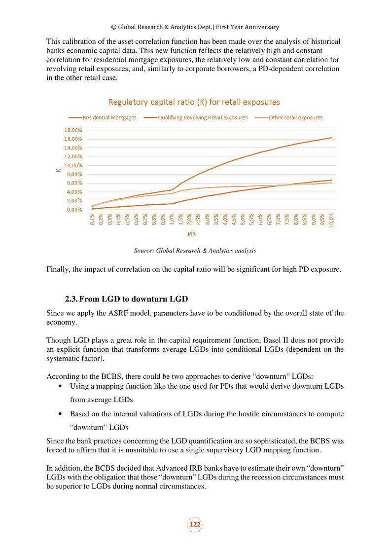
© Global Research & Analytics Dept.| First Year Anniversary
122
This calibration of the asset correlation function has been made over the analysis of historical banks economic capital data. This new function reflects the relatively high and constant correlation for residential mortgage exposures, the relatively low and constant correlation for revolving retail exposures, and, similarly to corporate borrowers, a PD-dependent correlation in the other retail case.
Source: Global Research & Analytics analysis
Finally, the impact of correlation on the capital ratio will be significant for high PD exposure.
2.3. From LGD to downturn LGD
Since we apply the ASRF model, parameters have to be conditioned by the overall state of the economy. Though LGD plays a great role in the capital requirement function, Basel II does not provide an explicit function that transforms average LGDs into conditional LGDs (dependent on the systematic factor). According to the BCBS, there could be two approaches to derive “downturn” LGDs:
• Using a mapping function like the one used for PDs that would derive downturn LGDs
from average LGDs
• Based on the internal valuations of LGDs during the hostile circumstances to compute
“downturn” LGDs
Since the bank practices concerning the LGD quantification are so sophisticated, the BCBS was forced to affirm that it is unsuitable to use a single supervisory LGD mapping function. In addition, the BCBS decided that Advanced IRB banks have to estimate their own “downturn” LGDs with the obligation that those “downturn” LGDs during the recession circumstances must be superior to LGDs during normal circumstances.
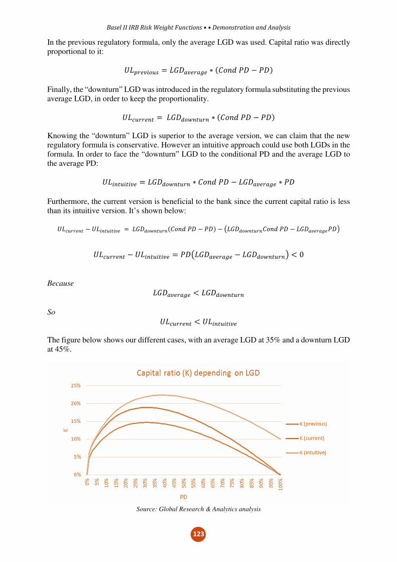
Basel II IRB Risk Weight Functions • • Demonstration and Analysis
123
In the previous regulatory formula, only the average LGD was used. Capital ratio was directly proportional to it: ÷õK89 .7!5 � õCöL 98L¤9 ∗ #p���"ö ( "ö' Finally, the “downturn” LGD was introduced in the regulatory formula substituting the previous average LGD, in order to keep the proportionality. ÷õ6!8891M � õCöD7"1M!81 ∗ #p���"ö ( "ö' Knowing the “downturn” LGD is superior to the average version, we can claim that the new regulatory formula is conservative. However an intuitive approach could use both LGDs in the formula. In order to face the “downturn” LGD to the conditional PD and the average LGD to the average PD: ÷õ.1M!.M. 9 � õCöD7"1M!81 ∗ p���"ö ( õCöL 98L¤9 ∗ "ö
Furthermore, the current version is beneficial to the bank since the current capital ratio is less than its intuitive version. It’s shown below:
÷õ6!8891M ( ÷õ.1M!.M. 9 � õCöD7"1M!81#p���"ö ( "ö' ( �õCöD7"1M!81p���"ö ( õCöL 98L¤9"ö�
÷õ6!8891M ( ÷õ.1M!.M. 9 � "ö�õCöL 98L¤9 ( õCöD7"1M!81� t 0
Because õCöL 98L¤9 t õCöD7"1M!81
So ÷õ6!8891M t ÷õ.1M!.M. 9 The figure below shows our different cases, with an average LGD at 35% and a downturn LGD at 45%.
Source: Global Research & Analytics analysis

© Global Research & Analytics Dept.| First Year Anniversary
124
At low PD, we notice a similar comportment between the current formula and the intuitive one. Moreover the current formula is easier to compute since it only depends on downturn LGD which could explain why this version was chosen by the Basel committee.
2.4. The maturity adjustment function
For two counterparties with the same degree of solvency, credit risk is not necessarily the same as everything here depends on the loan maturity. With the same degree of solvency, the higher is the loan maturity, the higher is the credit risk.
Since this maturity affects credit risk, it was necessary for the Basel committee to take it into account and adjust the capital charge formula.
According to the BCBS, there are 3 ways to consider the maturity adjustments:
The first one is considering the maturity adjustments as a consequence of increasing credit risk. The fact that credit risk increases with increasing maturity has to imply more capital charge (loan maturity effect).
The second one is considering the maturity adjustment as an anticipation of additional capital charge due to downgrades. Indeed, downgrades are more likely when it comes to long-term credits and hence the anticipated capital charge will be higher than for short-term credit (potential downgrades effect).
The third one is considering the maturity adjustments like a consequence of mark-to-market (MtM) valuation of credits. The expected losses are taken into account by investors when pricing the fair value of loans. Those expected losses are increasing with ascending PDs and decreasing with descending PDs. Therefore, the market value of loans decreases with increasing PDs and increases with decreasing PDs (marked to market losses effect).
For these reasons the BCBS integrated a maturity adjustments function to the basic regulatory formula to take into account maturity effects: loan maturity, potential downgrades and marked to market losses.
The maturity adjustments function is a function of both maturity and PD, and they are higher (in relative terms) for low PD than for high PD borrowers. The BCBS assumed a standard maturity of 2.5 years, so they constructed the function around this standard maturity. It’s presented as follows:
{é � 1 + #{ − 2.5's#"ö'1 − 1.5s#"ö'
��ℎ �ℎ �a���ℎ � a������ ��/���a ��: s#"ö' � #0.11852 − 0.05478 log#"ö))E
The figure below shows the maturity adjustment as a function of PD and maturity, reflecting the potential downgrade effect and the loan maturity effect.

Basel II IRB Risk Weight Functions • • Demonstration and Analysis
125
Source: Global Research & Analytics analysis
It’s worth mentioning for loan maturity less than one year, the adjustment increases with increasing PD but is still lower than 1. Consequently, the capital charge is lower than the case without maturity adjustment. For maturity longer than one year, the adjustment decreases with increasing PD but is still greater than 1, and consequently the capital ratio is also greater than the case without maturity adjustment.
Considering the maturities adjustment curves, we can wonder how the capital ratio is impacted by the maturity adjustment. The figure below shows the capital ratio as a function of PD and maturity thus considering the maturity adjustment.

© Global Research & Analytics Dept.| First Year Anniversary
126
Source: Global Research & Analytics analysis
We observe the behaviour of the capital ratio curve remains the same whereas it’s supposed to be proportional to the maturity adjustment coefficient. This can be explained because both the capital and maturity adjustment ratios depend on the PD. Thus the capital ratio curve maintains its state and is linearly dependent on the maturity only.
Source: Global Research & Analytics analysis

Basel II IRB Risk Weight Functions • • Demonstration and Analysis
127
2.5. A confidence level at 99.9%
According to the BCBS, the benchmark for setting the confidence level is BBB+ firms that have a default probability fixed on average at 0.1%, which amounts to say that the probability of survival is set at 99.9%. In other words, the BCBS is confident on average at 99.9% that a BBB+ rated bank would survive in the time horizon of 1 year. That’s why the confidence level is set at 99.9%. It means a bank can have losses that exceed its tier 1 and tier 2 capital on average once in a thousand years. Moreover it was also chosen to protect against estimation errors, which might inevitably occur from banks’ internal PD, LGD and EAD estimation, as well as other modeling uncertainties. Even if a bank is below the BBB+ rating, it has to respect the 99.9% confidence level. Nowadays most of the banks are above the BBB+ rating so currently the fixed confidence level is permissive, although this wasn’t always the case during the implementation of Basel agreements. In the future, we can expect an increase in confidence in order to better match the actual economy and its evolution. However, a decrease in confidence could be caused by a critical and massive downgrading of the banking sector. The figure below shows capital ratio measurement for different confidence level.
Source: Global Research & Analytics analysis
Formally, economic capital increases with increasing confidence levels. The higher the confidence level; the higher the economic capital is and vice-versa.
2.6. The standard normal distribution in the ASRF framework
The statistical properties of the Normal Law allow the Basel Committee to provide a closed formula for the regulatory RW calculation. Such properties remain a strong hypothesis of the ASRF model (as it exists on the market risk approach). These are reminded hereafter:

© Global Research & Analytics Dept.| First Year Anniversary
128
Indeed, let AÔ be the value of a borrower assets, described by the process:
�é � %é�� , eé�0 Where asset value at T can be represented as:
log é#�' � log é , %� ( 12e2� , e√�&
And X is a standard normal variable. We explained in part one that an asset i defaults if its value goes below a critical threshold¡.. Such as �. � ℙ#é. �p.' � ℙ#& t ¡.' � ϕ#¡.' Where
¡. � log p. ( logé. ( %� , 12eE�e√�
ϕ#. ' is a cumulative normal distribution function.
The variable X is standard normal, and can therefore be represented as
& � üû.� ,ü#1 ( û.'ý. � v. Where Y and εi are mutually independent standard normal variables, and are the risk factor
presented in part one.
Hence it explain the standard normal distribution used in the ASRF framework.
2.7. Processing portfolios default
Once default is observed, loss distribution is bimodal. In the cases that appear, almost all or nothing is recovered. The figure below shows the loss distribution in case of default.
Source: Global Research & Analytics analysis

Basel II IRB Risk Weight Functions • • Demonstration and Analysis
129
For defaulted portfolios PD is equal to 100%, and as a consequence, risk weight functions are not measurable. Hence expected loss and unexpected loss have to be recalculated together with LGD on defaulted exposures. Expected losses for defaulted portfolios depend only on expected recuperations on defaulted exposures. This best estimation of expected loss is called BEEL. Specific provisions are here to cover the BEEL. While default LGD is more severe than normal LGD, it’s supposed to estimate a downturn effect. The measurement of unexpected losses relies on the difference between loss recovery and their best estimation. It’s estimated as follows: ÷õ � max�0; õCöD9&L
© Global Research & Analytics Dept.| First Year Anniversary
130
Conclusion
After reviewing the funding principles behind Basel II and explaining the construction of risk weight functions, we exhibited input parameters of the function and detailed their limits, calibrations and impacts over the capital charge coefficient. The capital ratio is mainly dependent on PD and LGD; when both of them vary at low levels, the capital ratio is stable. High variations will occur when there are higher levels of these parameters, especially LGD since the ratio is directly proportional to it. Others parameters behind the Basel regulatory formula can explain a large number of adjustments made by financial institutions in the implementation of Basel II. In this sense, the assumptions and shortcuts decided in the regulatory RWA calibration need to be known and understood. In return, this would help banks refine their vision of economic capital and to better measure their actual risk (defaulted portfolio, financing cost of capital for SME, impact of systemic risk actually found in their own jurisdiction...). To conclude, having an in-depth understanding of the theoretical foundations behind the Basel formula will allow for opportunities to better address weaknesses and to help to uncover unexpected risks of banks.

Basel II IRB Risk Weight Functions • • Demonstration and Analysis
131
Bibliography
BCBS, 2004 “An explanatory note on the Basel II IRB risk weight functions” October
BCBS, 2005 “An explanatory note on the Basel II IRB Risk Weight Functions” July.
BCBS, 2006 “International convergence of capital measurement and capital standards. A revised
framework” June
C. Bluhm, L. Overbeck and Wagner C. 2003 “the introduction of credit risk modeling” Chapman and
Hall/CRC (1st edition) June
G. M. Gupton, C. C. Finger, and M. Bhatia. 1997 “CreditMetrics –Technical Document”. Morgan
Guaranty Trust Co.
A. Hamerle, T. Liebig and Rosch D. Discussion Paper “Credit Risk Factor Modeling and the Basel II
IRB Approach” Deutsch Bank series 2: Banking and Financial Supervision No 02/2003.
M. Crouhy and al. 2000 “A comparative analysis of current credit risk models” Journal of Banking &
Finance 24 59-117
P. Crosbie. 1999 “Modeling default risk”. KMV Corporation
Altman, E. I. (1968). Financial Ratios, Discriminant Analysis and the Prediction of Corporate
Bankruptcy. Journal of Finance 189-209.
Altman, E. I. (2000). Predicting Financial Distress of Companies: Revisiting the z-score and Zeta®
models. Retrieved 19 August 2009.
Allen and Powell, Credit risk measurement methodologies Bank for international Settlements. (2011).
Long-term Rating Scales Comparison. Retrieved 1 June 2011.
Bharath, S. T., & Shumway, T. (2008). Forecasting Default with the Merton Distance-to-Default
Model. TheReview of Financial Studies, 21(3), 1339-1369.
Crouhy, M., Galai, D., & Mark, R. (2000). A comparative analysis of current credit risk models.
Journal of Banking & Finance 24 59-117
D'Vari, R., Yalamanchili, K., & Bai, D. (2003). Application of Quantitative Credit Risk Models in
Fixed Income Portfolio Management. Retrieved 16 August 2009.
Du, Y., & Suo, W. (2007). Assessing Credit Quality from the Equity Market: Can a Structural
Approach Forecast Credit Ratings? Canadian Journal of Administrative Sciences, 24(3), 212-
228.
Grice, J., & Dugan, M. (2001). The Limitations of Bankruptcy Prediction Models: Some Cautions for
the Researcher. Review of Quantitative Finance and Accounting, 17(2), 151-166.
Gutzeit, G., & Yozzo, J. (2011). Z-Score Performance Amid Great Recession American Bankruptcy
Insitute Journal, 30(2), 44-46.
Huang, M., & Huang, J. (2003). How Much of the Corporate-Treasury Yield Spread is Due to Credit
Risk Unpublished Manuscripy, Stanford University.

© Global Research & Analytics Dept.| First Year Anniversary
132
Jarrow, R. A. (2001). Default Parameter Estimation Using Market Prices. Financial Analysts Journal,
57(5),75.
Jarrow, R. A., Lando, D., & Turnbull, S. (1997). A Markov Model for the Term Structure of Credit
Spreads. Review of Financial Studies, 10, 481-523.
Kealhofer, S., & Bohn, J. R. (1993). Portfolio Management of Default Risk. Retrieved 11 June 2009.
Lechner, A., & Ovaert, T. (2010). Techniques to Account for Leptokurtosis and Assymetric Behaviour
inReturns Distributions. Journal of Risk Finance, 11(5), 464-480. Moody's KMV Company.
(2003). RiskCalc Australia Fact Sheet. Retrieved 11 June 2009.
Ohlson, J. A. (1980). Financial Ratios and the Probabilistic Prediction of Bankruptcy. Journal of
Accounting Research, Spring, 109-131.
Pesaran, M. H., Schuermann, T., Treutler, B. J., & Weiner, S. M. (2003). Macroeconomic Dynamics
and Credit Risk: A Global Perspective. Retrieved 1 June 2011.
Sy, W. (2007). A Causal Framework for Credit Default Theory: APRA, wp08-03.
Sy, W. (2008). Credit Risk Models: Why They Failed in the Financial Crisis: APRA, wp0803.


