A wake model for free-streamline flow theory Part 2. Cavity flows past obstacles of arbitrary profile

In I'art 1 of this paper a free-streamline n ukc model mas introtlueed to treat the f'ally and partially developed wake flow or. cavity flow past an oblique flat plate. This theory is generalizetl l~crc to investigate the cavity flow past an obstacle of arbitrary profile a t am arbitrary cavitatioti nurnli~er. (:onsicicration is first given to the cavity flow pai t a polygond obst;~cle whose 14 etted sides may be concave towards the flow and may also possess some gentle convex corners. The geiieral case of cur\ cd walls is t l ~ c n obtained by a limiting process. The analysis in this general caw leads to a set of two -CLlnctiol~>~I eyuatiolis for which several ~ l l c t l~ods of solutioii are tlcvelopcd a i ~ d discussed.

As a few typictbl examplcs tlie analysis is carried out in dctail for the specific cases of wcdges, two-step wcclgcs, flappet1 hydrofoils, anct inclined circular arc plates. Fora these cases the pt~csent theory is found to be in good ugreemcilt with the cxperimcntal results available.

1. Introduction The general t heory of potcr~tial liows past curvcd obstacles wit11 a free bouudarp

formatioil has bceii long recogilizcd as an iiiteresting but tlifictxlt mathematical problern. 'l'he qutlstioils of' coiistructiou. calculation, as well as cxistcncc anil uniqueilcss have ilitrigucd inanr outstallding hydrodynanlicist .; and inathcmati- ciaiis alike. The celebrated work of Lcvi-Civita (1907) for thp ilifiiiite cavity casr. has provitlcd thc basis for. the gcne~.al t,hoory by iiitrodtrci~lg a co~rvellient para- metrization of the ijow by which the solutio~l is exl)rcsscd in terms of' at1 arbitrary analytic fuiruction in s half unit circle, and thereby removing the unknowii hee boundary from tlle quc~stioii. Lovi-Civita's rcpresentaticil~ llas becii furtller advanced k)y Villat (19 1 I ) \I lio forrnulatcd the flow prohlclti in terms of functional integral cyuatiolii; which havc j)layccl a c c ~ ~ t r a l rolr in the c.xistcilcc theory arid the actual construd,ion of the sol l~ t io t~ . 1)i~tailetl discussions of' these funclameiital articles and tlie related dcvclop~lle~~ts call be fourld ill the recent literature oil this subject, for c~xainplc, (2ilbai.g ( I O f j O ) , I3irkhoff Ks Zaratitoirc~llo (L957).

It has bee11 lictticed that perhaps tlie most conlplex and difficult problem of' all is the actual coniputation of thc holution. Some practical aspects of these difti- cultics have bc1c.n discussed hy Rivkhoff 6L %arailtonello (chapter $1). 'I'his problein is largely unavoidak~le since fi~r cavity tloms past curveti ol)stacles, ever1 witlt infinite cavities, iluincrieal methotis s:>cm to be thc oiily iiieans of obtailling

f l~' i11ltl 121~c . l l 1 S

66 T. Yao-tsu W u and D. P. Wang

an accurate solution from the exact theory. While several finite-cavity flow models have also been considered together with the corresponding functional equations of Villat's type (see, e.g., Gilbarg 1960), the incorporation of these models only magnifies the complexities of the computation. One approximate method in common use is to make the continuous curvature equation discrete by a polynomial representation and to solve the resulting set of equations by direct iteration. However, this iteration has been shown to diverge for large values of a certain parameter M (which relates the scale of potential and that of the physical plane); for such cases a more elaborate averaged iteration has been introduced by Birkhoff, Goldstine & Zarantonello (1954). Prom our experience, the difficulties become particularly noticeable in the case of thin curved barriers held at small incidences to the flow since the total variation of the integrand in the functional equations increases rapidly with decreasing angle of attack. Un- fortunately, this is also the case of considerable interest from the viewpoint of practical applications, such as cavitating hydrofoils and stalled airfoils. In short, i t seems that so far none of the general iteration methods have been rigorously proved to converge, and theoretical estimates of error are still lacking.

The main objectives of this paper are twofold: (1) to develop an exact theory for the general case of arbitrary body profile and arbitrary cavitation number by adopting a rather simple wake model and by using a different para- metrization, (2) to examine various numerical schemes which can be applied uniformly in the incidence angle and the cavitation number.

In part 1 of this paper (Wu 1962) a free-streamline wake model was intro- duced to treat the flow past an oblique flat plate with a fully or partially developed wake (or cavity) formation. According to this model the wake flow is approxi- mately described i11 the large by an equivalent potential flow past the body with an infinitely long wake which consists of a near-wake of constant under-pressure and a far-wake trailing downstream. The pressure increases continuously back to its free-stream value along the far-wake boundary which is assumed to form a branch slit of an unknown shape in the hodograph plane.

This theory will now be generalized to evaluate the wake (or cavity) flow past an obstacle of arbitrary profile a t arbitrary cavitation number. Consideration is first given to a polygonal obstacle whose wetted sides may be concave towards the flow and may also possess some gentle convex corners. The parametric plane of the flow is chosen to be in a half unit circle, with the circular arc corresponding to the constant pressure free boundary and the diameter to the wetted surface in such a way that this plane becomes the hodograph as the polygon is degenerated to a flat plate. The general case of curved walls is then deduced by a limiting process. The analysis in this general case leads to a set of two functional equations which are quite similar to Villat's equations. These equations immediately provide the exact solution of a wide class of 'inverse problems'. While the general direct problems are still difficult to solve exactly, the computation of the present theory is, however, not further complicated by non-vanishing cahtation numbers (aside from the determination of an additional scalar parameter). Several numerical methods for the general purpose have been developed here, some of which have already been applied with success.

Wake model for free streamline$ow. Part 2 6 7

In order to exhibit some salient features of cavity flows past curved obstacles, such as the effects of camber, cavitation number, incidence angle, and so forth, as well as to achieve a sound grasp of the convergence of various numerical schemes, the analysis and the subsequent computation have been carried out in detail for several typical examples: wedge, two-step wedge, hydrofoil with a flap, and inclined circular arc plate. The methods adopted have been found to converge in every case tried. Furthermore, in these cases the present theory is found to be in good agreement with the experimental results available.

2. Cavity flows and wake flows past a polygonal obstacle We consider first the steady, plane, potential flow of an incompressible fluid

past a polygonal obstacle with a wake or cavity formation in such a way that the fl sides of the polygon are wetted and the flow is separated from fixed leading and trailing edges A and B, forming two free streamlines ACI and BC'I, as shown in the physical plane z = x + iy of figure 1. The free stream a t infinity is inclined a t an angle a with the x-axis which may be chosen (but not necessarily) to coincide with the chord AB. Let z, = z,, z,, z,, ..., z, = z, be the vertices of the polygon; and let (1 + s,) 7r be the exterior angle (on the cavity side) subtended by the consecutive sides a t z,~, k = 1,2, . . . , (N - 1).

The polygonal wall may be concave towards the flow and may also possess some gentle convex corners so long as the resulting flow configuration provides a valid approximation of the actual physical flow. It is noted that the potential flow a t such a convex corner, if not a stagnation point, must be singular there. Whether the flow is actually separated or not from such convex corners, however, should be investigated by including the relevant real fluid effects such as the viscous boundary layer a t the wall, convection and diffusion of dissolved gases, as well as other properties of incipient cavitation. These real fluid effects are rather complicated and difficult to be taken into an accurate account; they will not be further discussed in this work. I n the present formulation the flow around such convex corners may be regarded as an approximation to the actual case in which either the real fluid effects under the circumstances keep the flow from being separated or there exists only a small separated bubble with an immediate reattachment to the solid surface, so that no serious error results from neglecting such detailed local structure of the flow. To permit such gentle con- vex corners to remain wetted in the cavity flow is essential when we later generalize this analysis by a limiting process for obstacles of arbitrary profile. With this additional degree of freedom, s, is positive or negative according as the boundary a t z, is concave or convex towards the flow. It should be emphasized, nevertheless, that due caution must be exercised and the possibility of change in the basic flow pattern considered (for small enough a the flow in figure 1 may change the separation point from B to z,, thus leaving z,B inside the cavity).

Adopting the same notation as in Part 1, we haye the complex potential f (2) = $ + i$, and the complex velocity

T. Yao-tsu Wu and D. P. Wang

f Y z-plane

P = PC P = P, p increases

from p, to pm I a

$

I f-plane

'I c-plane A

D Im t t-plane

Re r

D

FIGURE 1. The free-streamline model for the wake flow past a polygonal obstacle and its conformal mapping planes.

The free stream has velocity U and incidence angle a, so

The general description of the present wake flow model has been given in Part 1, which may be summarized here for the convenience of subsequent applica- tion. The part AC and BC' of the free streamlines form the lateral boundary of a near-wake of constant pressure

p = pc < p, on AC and BC', ' (3)

p, being the free-stream pressure. From this part onward p varies continually and monotonically from pc top, along the far-wake boundary, C I and C'I. I t is further assumed that fc = fc,, wC = wc.

(4)

Wake model for free streamlinejlow. Part 2 69

Moreover, the images of the free streamlines C I and C'I are assumed to form a branch slit of undetermined shape in the w-plane (the hodograph-slit condition). The Bernoulli equation of the external flow is

where q, is the constant value of q along AC and BC'. With q, normalized to unity, we have qc = lj u = (1 + g)-%, (6 a)

where g = ow -r),)l(&pu2), (6 b)

g being the wake under-pressure coefficient, or the cavitation number for cavity flows. Condition (3) is written for the case of full wake flow; for the partial wake flow case (see Part 1 for further details) the constant pressure portion BC' behind the trailing edge B then disappears.

For the present problem we introduce the < and t parameter planes by

where A is a positive real constant and the complex constant C0 is the image point (yet undetermined) of z = CQ. The flow regions in the < and t-planes are shown in figure 1. The local conformal behaviour a t C and C' requires that

dfld< = O(I<-<GI) as I<-<cI+O, from which it follows that

cc = cct = Reco:,. (9 a)

Moreover, the line segments CI, C'I and D I are seen from (7) to be straight lines parallel to the Im <-axis. The fully cavitating flow is again specified by the condi- tion that the point C' falls downstream of the trailing edge B, or

When the numerical result gives Reco :, 1, the flow may be supposed to have undergone transition to become partially cavitating.

Equations (7) and (8) can be combined to give

f (t) = At2[(t - to) (t - fo) (t - t; l) (t - f;1)]-17 (10)

where to, from (8), is given by to = C0- (<;- I)*. The use of the variable t is sug- gested by the analysis of Part 1 : here t plays the role of the variable w of the wake flow past an oblique flat plate (see Part 1) so that with t = w, (10) provides the required solution of the flat-plate problem.

The solution of the present problem is seen to be best represented in the para- metric form f = f(t) and w = w(t). We proceed now to determine the latter part w = w(t). Let the points T ~ , T ~ , . . . , T ~ - ~ on the real diameter of the t-plane ( - 1 < T~ < T~ < ... < T ~ - ~ < 1) correspond to the vertices z17z2, ... ,z,-, of the wall. We further let the stagnation point D, a t which w = 0, be chosen a t t = 0. Now, as the point z moves along the polygonal boundary from A to B, Im(1og w) = arg w remains constant on every straight segment, jumps by ( skn)

70 T. Yao-tsu Wu and D. P. Wang

as z moves across the vertex z,, and jumps by 71 as z goes over the stagnation point. Furthermore, along AC and BC', where It 1 = 1, we have

Re (log w) = log qc = 0.

From these two conditions one sees by inspection that

where Po is the angle made by the leading segment with the x-axis, positive in the counterclockwise sense. It is obvious that the above w satisfies the conditions on arg w over the solid boundary. Furthermore, with - 1 < T < 1 and S real, the conformal transformation

T = exp (is) (t - T ) / ( T ~ - 1) ( l l a )

maps the circle It1 = 1 on IT1 = 1, and we have IT/ < 1 when It1 < 1. This establishes the solution (11). I n particular, when Po and all s, vanish, w and t become identical, leaving (10) as the known solution of the flat-plate problem (see Part 1).

Equations (10) and (11) give the parametric solution f = f(t), w = w(t). The solution is completed when the physical z-plane is determined from

z(t) = dfdt. Ill w(t) dt

The above integral cannot in general be integrated in a closed form. It is noted that the solution given by ( lo) , (11) and (12) contains ( N + 1) para-

meters A, to, T ~ , . . . , T ~ - ~ (N + 2 real parameters as only to is complex) which can be determined by the following consideration. First, a t z = oo, or t = to, application of condition (2) to (11) yields

The region of Itol for the particular case of all s, > 0 can be seen from (13), ( l la ) to be

U < Ito\ < 1, ifall s, > 0. (134

Furthermore, the length of the kth segment is

( k = l , 2 ,..., N). (14.1

Finally, we also have

where 1 is the chord length and a, the inclination of the chord. Equations (13) and (14) form (N + 1) equations, which are in general non-linear and transcendental, for the (N + 1) parameters A, to, T ~ , . . ., TN-~. For further discussion on the deter- mination of these parameters, we distinguish between the following two cases.

Wake model for free streamline$ow. Part 2

3. The direct and inverse problem; numerical iteration methods The original physical or direct problem is specified with prescribed geometry

(all 1, and ek given) and flow configuration (a! and the cavitation number o or U given), there being a total of (2N + 1) direct physical parameters,

A wake flow past a N-sided polygon can therefore be represented by a point P in a (2N+ 1)-dimensional space with the above co-ordinates. The region of these co-ordinates permissible for our physical problem may be described as

where SIC, the lower limit of elc, may be zero or may assume some small negative value (in order to render a valid approximation of the actual motion, as explained earlier). Aside from this qualifying condition, no definite lower bound of the negative value can be stated in general for SIC. If, however,

then the wetted surface is concave to the flow. On the other hand, our solution given by (10)-(14) also defines a wake flow past

a N-sided polygon which can be represented by (2N+ 1) 'inverse flow' para- meters

Pf(A; to (complex); r,, . .., TN-,; el, .. ., B ~ - ~ ) , ( 1 7 ~ )

with the corresponding region

For the more restricted case of SIC = 0 in (16 b) and (17 b) the corresponding region will be denoted by R, and Ri . For definiteness some statement in the sequel will be made on the basis of the region R, and R i since the relaxed case when e, may assume small negative values must eventually depend on experimental verifi- cation.

Let us consider the inverse problem by choosing a point P' within the region Ri . Then, since Irk\ < 1 and Itol < 1, i t follows from (13) that

so that o = (U-2- 1) > 0. Equating the argument of (13), we obtain the incidence (a! - Po) of the leading segment

N-1 a - Po = - arg to + 2 elc[arg (rlt to - 1) - arg (to - r,)].

l c = l (18b)

The entire configuration is then fixed (up to a common scale factor A), with the length 1, of every segment given by (14). Therefore, to each P' in R i there corresponds a single Pi l l R,. I n this sense we may assert that the mathematical solutioii of an inverse problem exists and is unique.

7 2 T. Yao-tsu Wu and D. P. Wang

In the direct problem with prescribed P , there are (N+ 1) unknown para- meters A; to; rl, . . . , rN-,, which have to be determined from the (N + 1) transcen- dental equations (13) and (14). These equations are in general very difficult to solve directly. The existence and uniqueness consideration for the original physical problem is to establish the converse statement that to each point P there corresponds one and only one P', or in other words that the (N + 1) non-linear equations (13) and (14) possess a unique solution of the (N + 1) unknown para- meters for any prescribed values of the physical parameters in P. The problem of existence and uniqueness may be treated by adopting the idea of 'local unique- ness' as used by Weinstein (1924, 1927, 1929), and Leray (1934, 1935) for similar problems in the theory of free-boundary flows. The details of such considerations, however, will not be pursued further in this work.

The above consideration of the inverse problem provides a basis of constructing approximate methods for the direct physical problem. We have essentially established two such methods: (i) an integral iteration scheme, and (ii) a dif- ferential perturbation approximation, both depending on a known basic flow as the reference. The difference between the actual flow and the basic flow need not be very small for the first method as long as the iteration converges, whereas this difference is assumed small for the second method to be effective. The integral iteration for polygonal obstacles is best presented as a special case of the general method for curved profiles; this is done in $5.1. We present below the differential perturbation method &it may also bear some interest regarding the problem of existence and uniqueness.

Suppose that a basic flow P(a ; a ; Z,, . . ., ZN; s,, . . ., sN-,) is given by (13) and (14) with prescribed parameters P'(A; to; r,, ..., TNV1; s,, ..., s,-,). Let these para- meters be given variations SA, SV, &ao, ST,, Ss,,, where to = Ve-iao. Then the corresponding variations of the physical parameters are given by

az. sl. = aA % s a + ~ s v + ~ s E ~ + av aa, (194

wherein(19a),j = 1,2, ..., N.In(19c)Umaybereplacedbyasincea = (U-2--1). The coefficients of the above set of (2N + 1) equations can be readily deduced by differentiation of (13) and (14); their explicit expressions will not be given here.

Conversely, if a physical flow is given by P, (a; a ; 1, + W,; s, + Ss,) which in turn may be regarded as a variation of the basic flow at fixed a and a , then the corresponding variation of the inverse parameters can be obtained by solping the (2N + 1) linear equations (19) with the known quantities SZ,, Ss,, SU = 0, Sa = 0, provided that the Jacobian

a(a; a ; z,, ..., zN; el, ..., eN-,)/a(~; V; ao; 71, ..., $I; 61, ..., CN-,) (20) is non-vanishing. The last statement would also imply existence and uniqueness.

Wake model for free streamlineJEow. Part 2 73

The above perturbation theory can be applied to construct an iteration scheme as follows. We combine ;he so determined variation (&A, 6V, 6a0, 6rlC, &el<) with the original reference flow to provide a new reference flow P;(A+GA, V+6V, a, +6a0, rk + 6rlc, elc + &el<) which, by using (13) and (14) as an inverse problem, povides in turn a new physical flow P, (a@), dl), lL1), &)). By comparison of P, with the given flow P, a set of new variations (601, 6c, WIG, 6elC) of the physical parameters is obtained, thus enabling one to proceed by repeating the process iteratively over and over again. Needless to say, the success of this iteration process depends on how fast the set P,(a(n), dm), lj:), ef22)) converges to the pre- scribed physical flow.

It may be remarked that the first reference flow need not have the same number N of faces. For example, when all the e,'s are small, the cavity flow past the flat plate spanning along the chord AB can be used as the basic flow, in which case the complex velocity w of the basic flow coincides with t, and r,, . . . , r,-, of the basic flow become the image in the t-plane of those points on the flat plate which are at the same length apart as the vertices of the given polygon (in other words, 61, are all chosen to be zero for the first iteration).

4. Obstacles with arbitrary profile; the functional equations The preceding results can be readily extended to contain the general case when

the obstacle has an arbitrary profile. This generalization is quite straightforward for the case ofJixed detachment when the detachment points (in general at sharp corners) are assumed known. The theory can also be applied to the problem of smooth detachment, when the detachment points (at a smooth surface, for example) cannot be prescribed in advance, provided some additional appropriate condi- tions are imposed for their determin ion. The condition generally adopted for this type of problem is based on d illat's criterion (1914) which requires the curvature of the free streamline to be finite at the point of smooth detachment.

Thus we presume that the free streamlines become detached from the body a t points A and B (with either fixed or smooth detachment) to form a wake or cavity, as depicted in figure 2. The wetted surface of the obstacle may be expressed parametrically as

x = x(s), y = y(s) for 0 < s < S, (21 a)

where S is the tola1 arc length of the wetted surface. These functions and their first derivatives may be assumed Holder continuous in s for 0 < s < S. The inclinatioil angle of the body surface with the x-axis is

Here the variation of p need not be limited to be small as long as the resulting flow is supported by physical observations. The maximum variationof P, defined as the difference between the maximum and minimum value of P, may be taken to be less than ?T and may be considerably smaller in ordinary cases of practical applications.

74 T. Yao-tsu Wu and D. P. Wang

Let us consider a limiting process by which the number N of the polygonal faces increases beyond all bounds, the face lengths lk all tend to zero, and the turning angles s, all become vanishingly small except possibly at a finite number of isolated points where the obstacle has sharp corners. In the limit as N + m and Isr 1 + 0, we may rewrite (1 1) as

N-1 t-Tk w = e-iPo t exp C s, log -- ( lc=l - JI

FIGURE 2. Free-streamlines with fixed akid smooth detachment from a solid boundary.

and then replace the summation by an integration with respect to the continuous variable r , substituting s,n by ( - dp) where P(T) is the inclination angle of the body surface at the point t = T. (The negative sign of ( - dp) is taken on account of the original convention of the positive sense of s,.) We therefore obtain

where clearly Po = P(- 1). It may be noted that this result includes the special case (11) for polygonal bodies when we take

S(T - T ~ ) being the Dirac delta function. Integrating the integral in (22) by parts, we find that the contribution at the lower limit T = - 1 (where P = Po and log [(t - T ) / ( ~ T - l)] = in) cancels the factor exp ( - ip,), giving

w(t) = texp -- ( (I nt2)/11 (r-t) p(T)dT (Tt- I) I The exact solution is therefore expressed parametrically as f = f(t), w = w(t), with f(t) given by (10) and w(t) by (22) or (23). As a remark, the above solution w(t) can also be obtained directly by the method of functional theory (see Appendix).

Wake model for Pee streamline $ow. Part 2 75

The form (22) is based on the curvature whereas (23), on the inclination of the body surface. In fact, the curvature of a bounding streamline, defined by K = d8/ds (s being the arc leggth along the streamline), can be written

where w = ilogw = 8+ih. (24 b)

Hence on the body, 8 = P (or they may differ by a t most a constant),

and on the cavity boundary where h = 0,

Finally, the physical 2-plane is again determined by (12), except now w(t) is given by (22) or (23). I n particular, on the body (t real),

in which * above the integral sign signifies the Cauchy principal value. Since for real t,

dr - = 0, f:l (r-t) (d- 1)

we may also write for the points on the solid surface, or for t real,

(1 - t2) P(r) - P(t) df dt 2(t) = / ~ l e i ~ ( t ) e x p ( T / -1 (r - t) (rt - 1) dr)- dt -. t (26b)

Since dz = (ds)eiP, i t therefore follows from (26b) that the arc length s(t) along the body surface, measured from the leading edge A, is

(1 - t2) P(r) -P(t) clf dt s(t) = 14, exP (7 1 - - dr - -.

-1 (7 - t) (rt - 1) 1 dt t

The above formal solution contains two arbitrary parameters A and to, and an arbitrary real function P(t). They are governed by the following conditions. First, application of condition (2) to (23) yields

Next, let us consider the bouildary condition on the solid surface. In the case of fixed detachment, the angle Pis a given function of s (see (21)). However, s(t) and hence P(t) = P(s(t)), which appear in (27) and (28), are not known a priori. Thus the right-hand side of (27) and (28) may be regarded as two integral operators 91[s(t), P(s); to] and 9,[s(t), P(s); to] depending on s(t), P(s) and the parameter to,

7 6 T. Yao-tsu Wu and D. P. Wang

which provide the functional transformations of s(t) into the left-hand side member of (27) and (28), or symbolically,

s(t)lA = $,[s(t), P(s(t)); to17 (29

ue-ia = $,[s(t), P(s(t)); to], (30)

the right-hand sides of these equations being independent of the parameter A. Equations (29) and (30) are a set of functional equations for the unknowns s(t; to), P(t) and to. Pinally, the parameter A is fixed by the physical scale of the total arc length s(1) = s. (31)

For the problem of smooth detachment, each smooth-separation point becomes ail additional unknown for which another condition must be imposed for its determination. We may adopt the finite curvature condition that

where o = ilogw, and where t = - 1 (or 1) is applicable when the smooth detachment occurs a t A (or B). This can be seen as follows. Prom the local con- formal behaviour of f(t) a t t = T 1 i t is obvious that dfldt vanishes like (t + 1) as It + 1 I + 0. Therefore the curvature of the free streamline (K, = doldf, see (25 b)) will be infinite a t the detachment unless doldt also vanishes there. In the latter case it follows from Villat's alternative (Villat 1914) that the curvature of the free streamline a t detachment coincides with that of the body. By using (23), condition (32a) can further be written

which must be used together with the previous conditions to determine P(s(t)), to and A. \

The above considerations provide a means of constructing inverse and approxi- mate solutions of the cavity problem. Por the inverse problem we begin with an adequate choice of to and the function P(t), then a and U (or rr) can be calculated directly from (28), and the geometrical configuration by quadrature from (26). Again, the body profile varies for different a and rr. The exact solution of an appropriate inverse problem can also be used as the reference flow for approxi- mate solutions of the original physical problem.

5. Numerical iteration and approximate methods The general profile of the curved obstacle may admit (N- 1) isolated sharp

corners across each of which (say a t 2,) the inclination ,8 jumps by ( - e,n) so that we may write N - 1

where s, is the arc length from A to z,, and H is the Heaviside step function. Clearly y(s) is continuous everywhere on the wetted surface. We present in the following two numerical schemes, the first one being entirely general, whereas the second is characteristic for a particular category of profiles.

Wake model for free streamlin.eJow. Part 2

5.1. An. integral iteration. method

The following integral iteration method has been developed for the general purpose and has been found to be relatively simple and straightforward to apply. Suppose there exists a known basic flow referred to which the flow in question may be regarded as a (not necessarily small) perturbation. For convenience the basic flow may be chosen as simple as practical; for example, one may chose an inclined flat plate if P(s) is everywhere small, or a two-sided wedge spanning the same end points A and B if P(s) is moderate or large. The exact solution of the basic flow will be denoted by

,8 = P(O)(s), s = dO)(t; t(O)), ti0), A(O). (34)

The function P(O)(s) is of course different from P(s) of (33). Equations (27) and (28) may be rewritten for the iteration scheme as

for n = 1,2,3, . . . , where (1 - t 2 P(7) - P(tl_

Here P(dm)(t)) assumes the corresponding value of the prescribed P(s) with s = dn)(t) for n. = O,1,2, . . . , s(O)(t) being provided by the basic flow. Other than this role, the inclination PcO)(s) of the basic flow never enters the iteration calcu- lation explicitly. Finally, the physical scale factor A(n) of each n. will be so chosen that d n ) ( l ) = S for n .=0 ,1 ,2 ,.... (39)

This condition ensures that the total arc length of the wetted surface in each iteration, including the basic flow, remains fixed (see condition (31)) so that the original boundary condition of the prescribed P(s) can be applied in the entire interval 0 < s < S. When the set of values {tim)) and functions {scn)(t)] tend to definite limits as n. + CQ, then this iteration converges to the required solution. I n numerical work, estimates of Is("+l)/s(",- 1 I and (tin+')/tim) - 1 1 provide a good indication of the rate of convergence.

I n the problem of smooth detachment one also has to apply the same iteration procedure to the additional condition (32 b), use of which must yield convergent values of the detachment points if the solution is to be meaningful.

It should be pointed out here that this iteration method is universal so long as the integral operations involved can be carried out and the process is convergent. It therefore includes the special case of step-jump P for polygonal obstacles.

5.2. Polyn.omia1 representation. of P(t)

Let us consider again the general case (33). While the determination of P(t) is generally complicated, the values of P are nevertheless prescribed for the fixed

78 T. Yao-tsu Wu and D. P. Wang

detachment points A and B, P( - 1) = PA, P(1) = P,, say. Hence from (33) y is also known a t t = + 1, namely

We may next expand the continuous function y(t) into a power series

1-t l + t (1 ;t)n ~ ( t ) = ? / ~ ~ + Y B T + C C Ymn - Y

m = l n=l (4 1)

which satisfies condition (40) and converges uniformly and absolutely for - 1 < t < 1. Furthermore, i t is noted from (25) that the curvature of the solid surface near the detachment points is -

dPldt - lim ~ ~ ( t ) = lim e"(&)---- dPldt - lim - t+* 11-01 1 dfldt t+*ldfldt'

But it has already been noted that (dfldt) vanishes like (1 + t) as 11 + tl +O. Therefore, as long as the curvature of the wetted surface is finite a t the detach- ment, regardless of whether the detachment is fixed or smool;h, the following two conditions,

- - 3 = 0 ( l i t ) as ll+t1+0, dt dt (434

must be satisfied, which, when applied to (41), yield

Actually we can carry out the limit in (42) and apply the known curvature conditions a t the detachment points; the result will however be omitted here.

An approximate method is obtained by taking a trun ated series in (41) with f M terms in rn and N terms in n. For simplicity we shall describe this method for the special case of no sharp corners, and hence P(s) = y(s). Substituting this polynomial in (27) and (28), we obtain

1 + t (1 - t2) y D I ~ ( r ) - y1V~(t) dr d f g, (44) s(t) = (E) exp["/ _I (r - t) (rt- 1) I dt t

where

I n addition to conditions (44), (45), we have of course conditions (43b), (31) and (32a) (the last one being for the smooth detachment case).

I n case the change of the surface inclination is sufficiently smooth over the entire surface, especially near the points A and B, one may regard

r(O)(t) = (Y - Y~WN)

Wake model for free streamlinejiow. Part 2 7 9

as the reference flow and derive a linear problem for the coefficients y,,,,. An appropriate number of points on the real t-axis may be chosen for application of condition (44).

6. Lift and drag The complex force F = X + i Y is seen to be

B

S dz F = iSA ( p - p ~ d z = t i p ( 1 - ww)dz = - t i p ( 1 -WE) - at, (47)

CABC' dt where the contour r is C'BAC. The first term of the last integral becomes

by integration by parts; and the complex conjugate of the second integral is

S dw wwdx = t i p wdf = +ip$ , fyd t .

CABC'

Now the integrands of the last twpntegrals are analytic and regular everywhere inside the contour r except at, the simple pole t = to. Since as t + to

we obtain by the theorem of residues

-

d log w

by using (2 ) . Finally, the lift L and drag D are given by

where G(t) = d log wldt, and hence for the polygonal obstacles

1 1 and in general G(t) = 1 t +L n [ [-- ( ~ - t ) ~ + -1 ( r t - p (r ) dr.

7. Some basic features of the free streamlines The shape of the free streamlines AC and BC' will now be determined. On the

boundary AC and BC' of the near-wake,

t = e-Zx (0 < X < 4, (51) which corresponds to 5 = [ = cosx. Then from (23) and (24 b)

80 T. Yao-tsu Wu and D. P. Wang

Let the image point of x = CQ be

t o - - Veciao, with O< V < 1, O < a o < r , (534

1 1 c0 = to + ino, to = (V + V) cos ao, no = - v sin a,, (53b) l ( l 1

with ltol < 1 for the fully developed wake flows. Then on AC and BC',

f = gA[(t- + nil-'. (54)

The curvature of AC and BC', by (25b), is K, = dwldf, or

2 d 1' (1 - P)$/~(T) d7) 2 [(t- to)' + nil2 ((1 - t2)-& K =- " A (6-60) 7fdt -1 72-2t7+1

(55)

Thus the curvature of AC and BC' is in general singular a t A, B, C and C'. The singular behaviour of the curvature a t C and C', or a t 5 = to, is an intrinsic feature of this wake model.

A parametric representation of the free boundary AC and BC' can be obtained from

( - l < t < t o ) , (56a)

where w ( t ) is given by (52).

8. Examples I n the preceding sections several numerical methods have beell developed for

the general purpose of evaluating the direct problems. I n order to exhibit the important physical effects of cavity flows past curved bodies and a t the same time to carry out these numerical schemes, we consider in the following a few typical examples: (A) symmetric wedges, (B) two-step wedges, (C) flat plate with a flap, (D) inclined circular arc. Case (A) contains only a simple integration; the com- plete result is presented here for possible adoptions as a reference flow for more complex problems. The general methods can often be considerably simplified for particular cases, such as shown in (B) and (C) where a combined use of the direct and inverse calculations can be made very effective and powerful. As a com- parison, the integral iteration method has also been applied to (C). Finally, the circular arc problem is solved by using the integral iteration method, and the results compared with the available experiments.

All the numerical computations have been programmed and carried out on the IBM 7090 computer a t California Institute of Technology. The errors involved in the computations, if explicitly verified, will be stated a t the relevant place.

(A) Symnzetric wedge

Consider the cavity flow past a symmetrical wedge of half vertex angle /3rr as shown in figure 3(a). The limiting case of infinite cavity a t g = 0 is known as Bobyleff's problem; and the problem with arbitrary g has been worked out with

Wake model for free streamline $ow. Part 2 81

various cavity models, e.g. with Riabouchinsky's model by Plesset & Shaffer (1948a, b), and Perry (1952), and with the wake model of Joukowsky and Roshko by Roshlco (1954). The method given here is essentially not different from that of

FIGURE 3. The co-ordinate systems and notations for spec5c cases.

Roshko who presented the numerical result for one case pn = 45". We derive here the final result in a closed form and present numerical values in a wider range.

By symmetry it is obvious that w = einBt2B. (57)

At z = a, w = U , hence to= - iV , V = Ul128= (l+a)-lHP. (58)

G Fluid Mech. 18

82 T. Yao-tsu Wu and D. P. Wang

consequently, from (10) f = At2(t2 + V2)-I (t2 + v-2)-1.

The physical plane is therefore

Let the length of one wedge face be 1, then

From (48), (50) we readily deduce that L = 0 and

D = v/3A V2(1- V4)-I (UU1 - U).

The drag coefficient based on the wedge base b = 21 sinpn is therefore

As G-aO, both U and V tend to unity, and we find the following asymptotic behaviour

where

471p2 csc p7I C G-

;P) 1+8py2(-p) [1+ G- + 0(g2)],

which can be expressed in terms of the logarithmic derivative of the I?-function. The above result for GD is computed and shown in figure 4 versus the cavitation

number G-for anumber of the vertex angles Pn. The present theory is found to be in good agreement with the experimental results of Waid (1957) and of Cox & Clayden (1958).

(B) Two-step symmetric wedge

Let us consider the cavity flow past a two-step symmetrical wedge with the inclination equal to /371 and (/3+ y )n on the first and second leg respectively (0 < /3 < 1, 0 < (/3 + y) < 1, see figure 3 (b)), the flow being again symmetric about the x-axis and the imaginary t-axis. Let t = f r correspond to the inter- mediate vertices, then w = ei"Bt2P(t2- r 2 ) ~ (7252 - I)-Y. (65)

A tx=co ,w = Uandt, = -iV, 0 < V < 1, hence

p = (V2+r2) / (1 +r2V2) , p (U/V2P)1'y. (66 a)

This equation may also be written

r2 = (p- V2)/(1 --pV2), or V2 = (p-r2)/(1 -pr2). , (66b)

Since 0 < r2 < 1 and 0 < V2 < 1, we deduce from (66b) that (i) V2 < p < 1 and (ii) r2 < p < 1. From (i) i t immediately follows that

UlI2P 3 V 2 U~/[~(P+Y)I for y = 0. (67)

Wake model for free streamline $ow. Part 2 83

(When y is negative, 1 yl is taken to be small compared with P.) This inequality gives the range of V for prescribed U = ( 1 +a)-*, and P, y. The inequality (ii) then provides an upper bound for r2.

FIGURE 4. Variation of CD with the cavitation number c for symmetric wedges. Waid's data: p?r = 5", 15O, 8 ; 45", V ; 90°, 0; the solid symbols represent the correspon.ding data obtained when the cavity was filled with a mixture of water and gas bubbles. Cox & Clayden data: p?r = 15O, 30°, 45", GO0, 90°, all represented by O.

The physical plane is given by

where

Let 1, and 1 , be the lengths of the segment DPl and Pl A, then

1 1-T2t2 Y 1 - 72t2 Y ST (=) t1-21g(t) dt = yT 1, 0 ( ) 72-t2 t 1 - g t ) dt.

84 T. Yao-tsu Wu and D. P. Wang

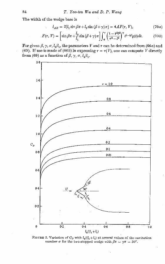
The width of the wedge base is

lA, = 2[11 sinpn + 1, sin (p+ y)n] = 4AF(r, V), (70a)

For given p, y, u, 1,/11, the parameters V and r can be determined from (66a) and (69). If use is made of (66b) in expressing r = r(V), one can compute V directly from (69) as a function of ,8, y, u, 1,/l1.

FIGURE 5. Variation of CD with 1,/(1, + I,) a t several values of the cavitation number a for the two-stepped wedge with pr = yr = 30'.

Wake model for free streamline $ow. Part 2

Finally, application of (50) to this case gives L = 0, and

Therefore the drag coefficient based on the base width is

FIGURE 6. Variation of CD with 1,/(1, +I,) at several values of tho cavitation number a for tho two-stepped wedgo with /3n = yn = 45".

86 T. Yao-tsu W u and D. P. Wang

A very straightforward scheme is adopted for the numerical computation in this case. For prescribed cavitation number CT (and hence U), a set of values of V are chosen within the region of (67), each of which then gives a fixed T by (66b). The ratio 1,/1, can therefore be calculated from (69) as a function of (U, V; ,8, y)

bla

FIGURE 7. Variation of CD with bla at several values of o- for the rectangular cup (or with P ~ T = y7~ = 90'). Waid's data for bla = 0.674 are compared with the theory in the inserted figure.

Wake mode2 for free streum2ine $ow. Part 2 87

from whioh readily follows the result for CD given by (72). No further elabora- tion is needed here as the numerical work involved is rather simple. The drag coefficient CD is shown versus 12/(2, + 1,) with fixed values of CT in figures 5-7 for three special cases: Pn = yn = 30°, 45' and 90". The last case has also been con- sidered by Plesset & Perry (1954). The agreement between the present theory and the experiment of Waid (1957) may be regarded as good, as shown in an inserted cross-plot of figure 7. The result that Waid's data are all slightly higher than the theory for b/a = co (for whioh case the flow is almost all stagnant inside the cup) may be due to the intrinsic feature of this flow model, or the wall effect which was not accounted for originally.

(C) Plat plate with a $up

As the simplest case of a polygonal obstacle in an asymmetrical flow we consider a flat plate APl with an extended flap PIB held a t a flap angle en whioh will be taken positive here (see figure 3(c)). With the x-axis taken along AP,, we have

w = t(t - r)e- (rt - l)-€, (73) where t = r is the image of the point PI. At z = co, w = Ue-i", t = to, hence

to = Ue-ia(l - ~ t , ) ~ (r - (74) From this equation it is readily seen that U < Ito 1 < 1 (or see (13 a)).

The physical plane is given by rt-1 e-

z(t) = 2~ I t (--) g(t; to) dt, -1 t-r ( 7 5 ~ )

1 df (1 - t2) [1+ t2 - #(to + to) (1 + t-lf-l)] where g ( t . t ) =-- = "0 ' O 2At dt (t - to)2 (t - to)2 (t - tr1)2 ( t i g 1 ) 2

' (75 b)

Let C and f* be respectively the unflapped chord and the flap length. Then

For convenience of computation, (76) can be written, by change of variables,

where

Finally, we derive from (50) for this case the lift and drag as

npA( U-l+ U) osc a, L =

2( V-2 + V2 - 2 cos 2a0)

(1 -r2) [(1 +r2) V2(1 + V2) - 2rV(1+ V4) cosa,] ( v ~ + T ~ - ~ ~ T c o s ~ , ) ( I + v 2 ~ 2 - 2 v r ~ ~ ~ a o ) ]

where to = V e-{"o.

8 8 T. Yao-tsu Wu and D. P. Wang

Equations (74) and (76) are two equations for to and r which can be solved numerically for prescribed U, a , e and f,/c. In the numerical computation the following different schemes have been adopted. The very nature of this special problem permits a combined use of iteration and the inverse problem calculation. If we choose U, a , e and r as the independent parameters (which are a mixture of the physical and inverse parameters), then to can be obtained from (74) by iteration?,

$,n) = U e-ia9-(thnn-1) ; r , e) for n = 1,2, . . . , (79 a) where 9-(to; r , e) = (1 - rtO)€ (r - to)-€, (79 b)

FIGURE 8. Variation of CL and CD with rr for a flat plate at incidence a = lo0, with a flap of flap-chord ratio f/c = 0.2 and held at flap deflexion en.

and t',O) may be chosen to be U e-ia. This computation was programmed for an IEM7090 electronic computer, and the iteration executed until an error of I tin) - tl;"-l)l< 0.000 1 is obtained. The convergence of this iteration is found to be very fast. With a series of r chosen in - 1 < r < 1, and with to so determined, the remaining parameter f,/c can then be determined readily from (76) or (777, and the lift and drag from (78). The accuracy of f,/c and L, D depend on the tin) used in the calculation, but otherwise their errors have not been explicitly deter- mined by using two consecutive values of tin). The numerical results of CL,and CD (based on the chord c) are first plotted versus f,/c (with the * deleted) for a set of values of a and en. From these figures the variation of CL and CD with a can be obtained by cross-plotting, a typical case of f/c = 0.2 being given in figure 8. The

t The iteration method is used here for the purpose of testing the rate of convergence.

Wake model for free streamline $ow. Part 2 89

special case of this problem with a = 0 has recently been treated by Lin (1961) using Levi-Civita's method. The corresponding numerical results of these two cases are found to be in perfect agreement.

FIGURE 9. Variation of CL with 0- for a circular arc hydrofoil a t incidence a.

It is easy to see that the above method (with T, chosen in order to calculate I,) soon becomes impractically complicated with further increase in the number of polygonal faces. For the purpose of comparison, this problem has also been calculated by applying the general integral iteration method as described in $5.1 which has been carried out on the IBM 7090 computer. It has been found that to obtain the same accuracy, the computer time for the integral iteration method is

90 T. Yao-tsu Wu and D. P. Wang

considerably more than that for the method mentioned above. It is felt, however, that the integral iteration method will likely be more advantageous and time- saving when there are more than two consecutive flaps.

0.7

Circular arc hydrofoil

0.5 -

0.4 -

C D

Parkin data o a = 10"

A '15' 0.1 - 0 20"

v 25" 0 30"

I I I I I I I I I 0 0.1 0.2 0.3 0.4 0-5 0.6 0.7 0.8 0.9 1.0

a

FIGURE 10. Variation of CD with a for a circular-arc hydrofoil a t incidence a.

(D) Circular-arc hydrofoil

As an example of the general profile with continuously varying inclination, we consider the circular-arc hydrofoil with radius R and arc length 2yR so that the arc angle is 2y (see figure 9). The inclination /3 is a linear function of s

P(s) = y - (SIR), 0 < s < 2yR. (80)

Wake model for free streamline $ow. Part 2 91

The problem has previously been treated by Wu (1956a) adopting the wake model of Joukowsky and Roshko and using Levi-Civita's method in an approxi- mate manner such that the series expansion is truncated and the boundary conditions on the inclination and curvature are satisfied only at the end points. The numerical work was carried out for y = 8" and the results compared with the experiments of Parkin (1956). The case of small y has also been considered by Wu (1956 b) as an example of the generalization of Tulin's linearized theory (1955) These two linear and non-linear theories have been compared for the case y = 8" (see Wu 1956b).

In order to compare the present cavity flow theory and the associated compu- tational program with the previous non-linear theory (Wu 1956 a), the numerical work of this problem has been carried out for y = 8", using the integral iteration method of $5.1 on a? IBM 7090 computer. In the computer program used in this case the conventional averaged-iteration process is employed. The iteration process is executed until the errors I Vn) - V(n-l)I and 1 akn) - abn-l) I are both less than 0.0001. The convergence of the iteration is considered to be very satis- factory. The resulting CL and CD (based on chord length l,, = 2R sin y) are shown versus (T in figures 9 and 10, in which Parkin's experimental data (1956) are included for comparison. The CD is found to be virtually identical with the previous approximate theory (Wu 1956a), whereas CL of the present theory is slightly greater than the previous one for moderate values of (T.

This work was supported by the U.S. Office of Naval Research under Contract Nonr 220 (35).

R E F E R E N C E S

BIRKHOFF, G., GOLDSTINE, H. H. & ZARANTONELLO, E. H. 1954 R.C. Semin. Mat. Torino, 13, 205-23.

B ~ K H O F F , G. & ZARANTONELLO, E. H. 1957 Jets, Wakes and Cavities. New York: Academic Press Inc.

Cox, A. & CLAYDEN, W. 1958 Cavitating flow about a wedge a t incidence. J . Fluid Mech. 3, 615-37.

GILBARG, D. 1960 Jets and Cavities. Handbuch der Physik, vol. IX, 311-445. Berlin: Springer-Verlag.

LERAY, J. 1934 C.R. Acad. Sci., Paris, 199, 1282. LERAY, J. 1935 Les probl6mes de representation conforme de Helmholtz. Comment. math.

helvet. 8, 149-80, 250-63. LEVI-CTVITA, T. 1907 Scie e leggi di resistenzia. R.C. cir mat. Palermo, 18, 1-37. LIN, J. D. 1961 A free streamline theory of flows about a flat plate with a flap a t zero

cavitation number. Hydronautics, Inc., Rockville, M d , Tech. Rep. no. 119-3. PARKIN, B. R. 1956 Experiments on circular-arc and flat-plate hydrofoils in non-

cavitating and full cavity flows. Cali$. Inst. Tech. Hydro Lab. Rep. no. 47-7 (see also 1955, J . Sh ip Res. 1 , 34-56).

PERRY, B. 1952 The evaluation of integrals occurring in the cavity theory of Plesset and Shaffer. Cali$. Inst. Tech. Hydro. Lab. Rep. no. 21-11.

PLESSET, M. S. & PERRY, B. 1954 Mdmoire sur la mecanique desJEuids offerts 6 M . Dimitri Riabouchinsky, pp. 251-61. Publ. Sci. Tech. Min. de I'Air, Paris.

PLESSET, M. S. & SHAFFER, P. A., Jr. 1948a Dragincavityflow. Rev.Mod.Phys.20,228-31. PLESSET, M. S. & SHAFFER, P. A., Jr . 1948b Cavity drag in two and three dimensions.

J . A p p . Phys. 19, 934-39.