A Wake Interaction Model for the CoordinatedControl of Wind Farms

Lin Pan, Holger Voos, Yumei LiInterdisciplinary Centre for

Security, Reliability and Trust,University of Luxembourg, Luxembourg

Email: lin.pan@uni.lu,Holger.Voos@uni.lu, yumei.li@uni.lu

Yuhua XuSchool of Finance,

Nanjing Audit University,Jiangsu 211815, China

Email: yuhuaxu2004@163.com

Mohamed DarouachResearch Center for

Automatic Control of Nancy(CRAN UMR, 7039, CNRS),University of Lorraine, France

Email: mohamed.darouach@univ-lorraine.fr

Lin Pan, Shujun HuSchool of Electric & Electronic Engineering,

Wuhan Polytechnic University,Wuhan, China

Email: hushj@whpu.edu.cn

Abstract—In all the processes of Wind Energy (WE) utiliza-tion, the Wind Power (WP) assessment is critical stage for all theWind Farms (WFs). This paper is focused on the WE systems inLuxembourg. It describes the overview of the wind resources inall the WFs and presents an Unified Cooperation Wake Model(UCWM) and Coordination and Optimization Control (CnOC)for WFs. Based on WP assessment of WFs, the statistical methodis used to model the distribution of wind speed and WindDirection (WD). Some simulation figures about the wind roseand Weibull distribution demonstrate the detailed description andassessment of WP. These assessments are expected to enhancethe effectiveness of WP exploitation and utilization in WFs ofLuxembourg.

I. INTRODUCTION

It is well known that WE is widely recognized to be oneof the most cost-efficient renewable sources of energy. Withthe increase of global wind-generation capacity in the lastfive years, WE has also become the fastest-growing electricalenergy in the world. In order to enhance the utilizationefficiency of WE, the most efficient way is to utilize existingWFs through improving control techniques and algorithms.At present, WE systems are being inclined to develop intolarge-scale distributed and coordination systems where thereare even more than eighty individual Wind Turbines (WTs)in operation. In contrast to the conventional power plants,e.g. nuclear power, thermal power, hydropower, etc. [1], [2],[3], [4], [5], [6], [7], these wind devices and equipment areexpected to operate and provide high quality power (Suchas: Safe, Stable, Controllable and Predictable (SSCP)) at thelowest possible cost.

In recent years, the research and development of WE har-vesting systems were focused on optimizing different aspectsof the WT in order to improve its Cost of Energy (CoE).Increase performance of the control system by optimizing theWT controller [1], [2] is one of the most important ways toenhance CoE of WT. WTs are often located in so called wind

parks or wind farms together with other turbines as so to reducecosts by taking advantage of economies of scale. Turbines inWFs can be located along a single line, in multiple lines, ingrids, in clusters or in configurations based on geographicalfeatures, prevailing WD, access requirements, environmentaleffects, safety, prior and future land use including ranch-landand farmland, and visual impact [3], [4].

Generally, the research on control of an array of WTsin WFs is more complex than control of single-WT settingbecause of the aerodynamic interactions among the array WTs.Therefore, the control on WFs is a more challenging research.In contrast to use single-WT control algorithms only, opti-mizing WP capture in WFs by coordination and optimizationcontrol of WFs will no doubt increase the utilization efficiencyof WE. The potential for improving performance and function,increasing WP capture as well as optimizing electricity loadsamong the WFs, have led to novel research efforts in coor-dination and optimization control of WFs. One method fordealing with these aerodynamic interactions is to develop anduse wake models in the distributed and optimization controlalgorithms. An alternative method is to develop an onlinecontrol approach where each WT adjusts its own inductionmodel coefficients in response to the information of localWFs, such as the WP generated by individual WT, local windconditions, local wind speed, local WD, local density of air,or interacted information regarding neighbor WTs. Here, thegoals are to develop coordination and optimization controlapproaches that permit the field of WTs to reach a desirableset of model coefficients, which will lead to better system levelbehavior, for example, WP maximization or electricity loadsminimization, without the need for complex modeling of theWFs [5], [6].

In view of Luxembourg locating in the western centralarea of European, and there are abundant wind resources totap into Luxembourg. There are currently more than 16 WFsestablished in the different places of Luxembourg. The list ofWFs in Luxembourg is shown in the table I [8]. As an example,978-1-4673-7929-8/15/$31.00 © 2015 IEEE

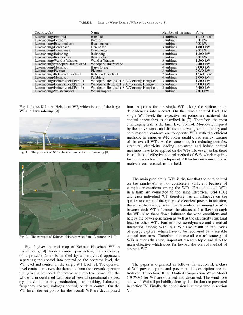
TABLE I. LIST OF WIND FARMS (WFS) IN LUXEMBOURG[8].

Country/City Name Number of turbines PowerLuxembourg/Binsfeld Binsfeld 5 turbines 11,500 kWLuxembourg/Boxhorn Boxhorn 1 turbine 800 kWLuxembourg/Brachtenbach Brachtenbach 1 turbine 600 kWLuxembourg/Derenbach Derenbach 3 turbines 1,800 kWLuxembourg/Doennange Doennange 1 turbine 800 kWLuxembourg/Reimberg Reimberg 2 turbines 1,200 kWLuxembourg/Remerschen Remerschen 1 turbine 600 kWLuxembourg/Wand a Waasser Wand a Waasser 3 turbines 1,500 kWLuxembourg/Wandpark Haardwand Wandpark Haardwand 4 turbines 2,400 kWLuxembourg/Mompach Burer Bierg 4 turbines 8,000 kWLuxembourg/Flebour Flebour 3 turbines 7,050 kWLuxembourg/Kehmen-Heischent Kehmen-Heischent 7 turbines 12,600 kWLuxembourg/Mompach Pafebierg 4 turbines 2,000 kWLuxembourg/Heinerscheid(Part 1) Wandpark Hengischt S.A./Gemeng Hengischt 3 turbines 1,800 kWLuxembourg/Heinerscheid(Part 2) Wandpark Hengischt S.A./Gemeng Hengischt 5 turbines 5,000 kWLuxembourg/Heinerscheid(Part 3) Wandpark Hengischt S.A./Gemeng Hengischt 3 turbines 5,400 kWLuxembourg/Weiswampach Weiswampach 1 turbine 2300 kW

Fig. 1 shows Kehmen-Heischent WF, which is one of the largeWFs in Luxembourg [9].

Fig. 1. The portraits of WF Kehmen-Heischent in Luxembourg [9].

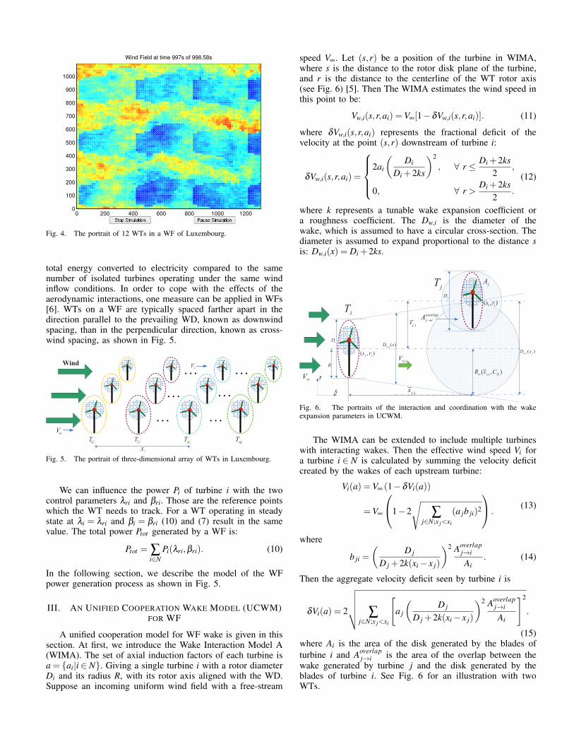
Fig. 2. The portraits of Kehmen-Heischent wind farm (Luxembourg)[10].

Fig. 2 gives the real map of Kehmen-Heischent WF inLuxembourg [9]. From a control perspective, the complexityof large scale farms is handled by a hierarchical approach,separating the control into control on the operator level, theWF level and control on the single WT level [7]. The operatorlevel controller serves the demands from the network operatorthat gives a set point for active and reactive power for thewhole farm combined with one of several operational modes,e.g. maximum energy production, rate limiting, balancing,frequency control, voltages control, or delta control. On theWF level, the set points for the overall WF are decomposed

into set points for the single WT, taking the various inter-dependencies into account. On the lowest control level, thesingle WT level, the respective set points are achieved viacontrol approaches as described in [7]. Therefore, the mostchallenging task is the farm level control. Moreover, inspiredby the above works and discussions, we agree that the key andcore research contents are to operate WFs with the efficientmethods, to improve WP, power quality, and energy captureof the overall WTs. At the same time, for reducing complexstructural electricity loading, advanced and hybrid controlmeasures have to be applied on the WFs. However, so far, thereis still lack of effective control method of WFs which requiresfurther research and development. All factors mentioned abovemotivate our research in the field.

The main problem in WFs is the fact that the pure controlon the single-WT is not completely sufficient because ofcomplex interactions among the WTs. First of all, all WTsin a farm are connected to the same Electrical Grid (EG)and each individual WT therefore has an influence on thequality or output of the generated electrical power. In addition,there are also aerodynamic interdependencies among the WTsbecause each WT influences the airstream that flows throughthe WF. Also these flows influence the wind conditions andhereby the power generation as well as the electricity structuralload on other WTs. Furthermore, aerodynamic and electricalinteraction among WTs in a WF also result in the lossesof energy-capture, which have to be recovered by a suitablecontrol measures. Therefore, the overall control strategy ofWFs is currently a very important research topic and also themain objective which goes far beyond the control method ofa single WT.

The paper is organized as follows: In section II, a classof WT power capture and power model description are in-troduced. In section III, an Unified Cooperation Wake Model(UCWM) for WF are obtained and discussed. The wind roseand wind Weibull probability density distribution are presentedin section IV. Finally, the conclusion is summarized in sectionV.

II. WT POWER CAPTURE AND POWER MODELDESCRIPTION

In this section, we introduce the control parameters of aWT by its induction coefficients which represent the fractionaldecrease in wind speed between the free stream conditions andthose seen at the rotor plane. For the optimization of a WF,it is too complex to model all the states of the WTs. Thewind model can been parameterize by the induction factors asopposed to more traditional control parameters, for example,tip-speed ratio and pitch angle, to provide a more compactrepresentation of the WF model. More specifically, the powergenerated by WT- i is characterized by the following equation[2].

Pi(ai,vi) =12

ρπR2v3i ηCP(ai)(λri,βri) (1)

where ρ is the density of air, R is the radius of WT, πR2 is thearea swept by the turbine blades, and vi is the average “inlet”wind speed for turbine i. The CP(ai) is the power efficiencycoefficient which takes on the form:

CP(ai) = 4ai(1−ai)2. (2)

In the equation (1), as a function of the reference values forthe Tip Speed Ratio (TSR) λri and the pitch angle βri withη = ηdηg representing the overall turbine efficiency:

λri =ωriRVi

(3)

ωri is the speed of the WT. The total power generated in theWF is simply:

Ptotal(a) = ∑i∈N

Pi(a). (4)

In order to obtain a sufficiently large correlation coefficientλri, we choose the mean density of air is 1.250kg/m3 inLuxembourg 2014, and the radius of WT as 66m for WF ofKehmen-Heischent in Luxembourg, and select the followingmathematical formula [11]:

Cp(λi,βi) =−0.2000+0.2000λi−0.007000βi

−0.020000λ2i +0.003000λiβi +0.000400β

2i

+0.000700λ3i −0.000200λ

2i βi−0.000100λiβ

2i

+0.000001β3i , i ∈ {1,2, · · ·}.

(5)

From the Fig. 3, we can see that function Power coefficientCp is very well fit with the variables: λ and β .

The dynamic representation of the WT in a switchedsystem has been investigated by authors in [4]. The dynamicmodel of the integrated system can be represented as:

ω̇ =1Jr(

π

8D2

r ρairCpv3

ω

ω− τGr) (6)

where Dr is the turbine rotor diameter, ρair is the density of air,vω is the input wind speed, ω is the turbine rotor speed, J isthe combined rotational inertia of the rotor, gearbox, generator,and shafts, Gr is the gearbox gear ratio defined as the generatorshaft speed over the rotor shaft speed, τ is the generator torqueand Cp is the power coefficient that measures how effectively

Fig. 3. The portraits of surfaces for power coefficient Cp with TSR λi, andpitch angle βi.

the WE is being converted to mechanical energy. It is a non-linear function of the blade pitch angle β and the tip speedratio λ :

Cp = f (λ ,β ). (7)

The tip speed ratio can be expressed as:

λ =ωDr

2Vω

. (8)

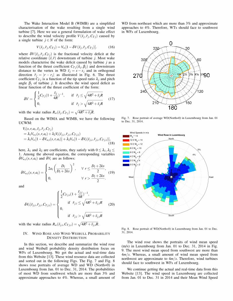
We locate 12 WTs as the position matrix in a WF with thesoftware SimWindFarm [12]:

[(x1,y1);(x2,y2); ...;(x12,y12)]

=[(0, 100);(400, 1000);(800, 100);(1200, 100);(0, 500);(400, 500);(800, 500);(1200, 500);(0, 900);(400, 900);(800, 900);(1200, 900)].

(9)

The local mean wind speed (m/s) is 3.2042m/s, the WTs’intensity is 0.1, WF’s length(m) is 1300m. WF’s width(m) is1100m, and Grid size (m) is 15m. The selected simulation time(s) is 1000s. By using the SimWindFarm Toolbox [12], we getthe following the portrait of 12 WTs in a WF of Luxembourgas shown in the Fig. 4.

Consider a one dimensional array of N identical WTs asshown in Fig. 5. Turbine Ti j is located downstream of turbineT1 j by a distance xi. The air flow velocity upstream of turbineT1 j is assumed to be uniform with speed defined as v∞. Itis further assumed that all turbines are perfectly aligned withthe direction of the upstream airflow, such that the air flowis orthogonal to each turbines plane of rotation. The powergenerated by the WF depends on the free-stream wind speedand the control actions of each turbine.

The mutual aerodynamic interaction of turbines in a WF isnot as well understood as the electrical interconnection of theturbines. While WFs help to reduce the average cost of energycompared to widely dispersed turbines due to economies ofscale, aerodynamic interaction among WTs can decrease the

0 200 400 600 800 1000 12000

100

200

300

400

500

600

700

800

900

1000

Wind Field at time 997s of 998.58s

Fig. 4. The portrait of 12 WTs in a WF of Luxembourg.

total energy converted to electricity compared to the samenumber of isolated turbines operating under the same windinflow conditions. In order to cope with the effects of theaerodynamic interactions, one measure can be applied in WFs[6]. WTs on a WF are typically spaced farther apart in thedirection parallel to the prevailing WD, known as downwindspacing, than in the perpendicular direction, known as cross-wind spacing, as shown in Fig. 5.

V

jT j

TnjTij

T

iX

iV

Fig. 5. The portrait of three-dimensional array of WTs in Luxembourg.

We can influence the power Pi of turbine i with the twocontrol parameters λri and βri. Those are the reference pointswhich the WT needs to track. For a WT operating in steadystate at λi = λri and βi = βri (10) and (7) result in the samevalue. The total power Ptot generated by a WF is:

Ptot = ∑i∈N

Pi(λri,βri). (10)

In the following section, we describe the model of the WFpower generation process as shown in Fig. 5.

III. AN UNIFIED COOPERATION WAKE MODEL (UCWM)FOR WF

A unified cooperation model for WF wake is given in thissection. At first, we introduce the Wake Interaction Model A(WIMA). The set of axial induction factors of each turbine isa = {ai|i ∈ N}. Giving a single turbine i with a rotor diameterDi and its radius R, with its rotor axis aligned with the WD.Suppose an incoming uniform wind field with a free-stream

speed V∞. Let (s,r) be a position of the turbine in WIMA,where s is the distance to the rotor disk plane of the turbine,and r is the distance to the centerline of the WT rotor axis(see Fig. 6) [5]. Then The WIMA estimates the wind speed inthis point to be:

Vw,i(s,r,ai) =V∞[1−δVw,i(s,r,ai)]. (11)

where δVw,i(s,r,ai) represents the fractional deficit of thevelocity at the point (s,r) downstream of turbine i:

δVw,i(s,r,ai) =

2ai

(Di

Di +2ks

)2

, ∀ r ≤ Di +2ks2

,

0, ∀ r >Di +2ks

2.

(12)

where k represents a tunable wake expansion coefficient ora roughness coefficient. The Dw,i is the diameter of thewake, which is assumed to have a circular cross-section. Thediameter is assumed to expand proportional to the distance sis: Dw,i(x) = Di +2ks.

V

overlap

j iAj ir

w j i TjR s C

iT

jT

j js r

j is

i is r

jA

s

r

w i jD x

w iV

iD

jD

w iD x

R

Fig. 6. The portraits of the interaction and coordination with the wakeexpansion parameters in UCWM.

The WIMA can be extended to include multiple turbineswith interacting wakes. Then the effective wind speed Vi fora turbine i ∈ N is calculated by summing the velocity deficitcreated by the wakes of each upstream turbine:

Vi(a) =V∞ (1−δVi(a))

=V∞

1−2√

∑j∈N;x j<xi

(a jb ji)2

.(13)

where

b ji =

(D j

D j +2k(xi− x j)

)2 Aoverlapj→i

Ai. (14)

Then the aggregate velocity deficit seen by turbine i is

δVi(a) = 2

√√√√√ ∑j∈N;x j<xi

[a j

(D j

D j +2k(xi− x j)

)2 Aoverlapj→i

Ai

]2

.

(15)where Ai is the area of the disk generated by the blades ofturbine i and Aoverlap

j→i is the area of the overlap between thewake generated by turbine j and the disk generated by theblades of turbine i. See Fig. 6 for an illustration with twoWTs.

The Wake Interaction Model B (WIMB) are a simplifiedcharacterisation of the wake resulting from a single windturbine [7]. Here we use a general formulation of wake effectto describe the wind velocity profile V (s̄ j, r̄ j,CT j) caused bya single turbine j ∈ N of the form:

V (s̄ j, r̄ j,CT j) =V∞[1−δV (s̄ j, r̄ j,CT j)]. (16)

where δV (s̄ j, r̄ j,CT j) is the fractional velocity deficit at therelative coordinate (s̄, r̄) downstream of turbine j. Most wakemodels characterise the wake deficit caused by turbine j as afunction of the thrust coefficient CT j(λ j,β j) and downstreamdistance to the vertex in WD s̄ j = s− s j and in orthogonaldirection r̄ j = |r − r j| as illustrated in Fig. 6. The thrustcoefficient CT j is a function of the tip speed ratio λ j and pitchangle β j of turbine j. It describes the wind speed deficit aslinear function of the thrust coefficient of the form:

δV =

12

CT j(1+s̄ j

4R)−1, if r̄ j ≤

√4R2 + s̄ jR

0, if r̄ j >√

4R2 + s̄ jR(17)

with the wake radius Rw(s̄ j,CT j) =√

4R2 + s̄ jR.

Based on the WIMA and WIMB, we have the followingUCWM:

Vi(s,r,ai, s̄ j, r̄ j,CT j)

= λ1Vw,i(s,r,ai)+λ2Vi(s̄ j,i, r̄ j.i,CT j,i)

= λ1V∞[1−δVw,i(s,r,ai)]+λ2V∞[1−δVi(s̄ j,i, r̄ j,i,CT j,i)],(18)

here, λ1 and λ2 are coefficients, they satisfy with 0≤ λ1,λ2 ≤1. Among the aboved equation, the corresponding variablesδVw,i(s,r,ai) and δVi are as follows:

δVw,i(s,r,ai) =

2ai

(Di

Di +2ks

)2

, ∀ r ≤ Di +2ks2

,

0, ∀ r >Di +2ks

2.

(19)

and

δVi(s̄ j,i, r̄ j,i,CT j,i) =

12

CT j,i(1+s̄ j,i

4R)−1,

if r̄ j,i ≤√

4R2 + s̄ j,iR

0,

if r̄ j,i >√

4R2 + s̄ j,iR

(20)

with the wake radius Rw(s̄ j,i,CT j,i) =√

4R2 + s̄ j,iR.

IV. WIND ROSE AND WIND WEIBULL PROBABILITYDENSITY DISTRIBUTION

In this section, we describe and summarize the wind roseand wind Weibull probability density distribution focus onWFs of Luxembourg. We get the actual and real-time datafrom this Website [13]. These wind resource data are collectedand sorted out in the following Figs. The Fig. 7 and Fig. 8shows rose portraits of average WD and WD (North=0) inLuxembourg from Jan. 01 to Dec. 31, 2014. The probabilitiesof most WD from southwest which are more than 3% andapproximate approaches to 4%. Whereas, a small amount of

WD from northeast which are more than 3% and approximateapproaches to 4%. Therefore, WTs should face to southwestin WFs of Luxembourg.

Fig. 7. Rose portrait of average WD(North=0) in Luxembourg from Jan. 01to Dec. 31, 2014.

Wind Speeds in m/s

WS ³ 14

12 £ WS < 14

10 £ WS < 12

8 £ WS < 10

6 £ WS < 8

4 £ WS < 6

2 £ WS < 4

0 £ WS < 2

Wind Rose in Luxembourg

1%

2%

3%

4%

5%

0% EastWest

North

South

Fig. 8. Rose portrait of WD(North=0) in Luxembourg from Jan. 01 to Dec.31, 2014.

The wind rose shows the portraits of wind mean speed(m/s) in Luxembourg from Jan. 01 to Dec. 31, 2014 in Fig.9. The most wind mean speed from southwest are more than4m/s. Whereas, a small amount of wind mean speed fromnorthwest are approximate to 4m/s. Therefore, wind turbinesshould face to southwest in WFs of Luxembourg.

We continue getting the actual and real-time data from thisWebsite [13]. The wind speed in Luxembourg are collectedfrom Jan. 01 to Dec. 31 in 2014 and their Mean Wind Speed

Fig. 9. Rose portrait of Wind Mean Speed(m/s) in Luxembourg from Jan.01 to Dec. 31, 2014.

(MWS) is 3.2042m/s. They are shown in the following Fig.10.

0 2000 4000 6000 8000 10000 12000 14000 16000 180000

2

4

6

8

10

12

14Wind speed time series in Luxembourg from Jan. to Dec. 2014

Time (30−minute sampling period)

Win

d s

pe

ed

(m

/s)

Wind Speed

Mean wind Speed

Fig. 10. The portraits of wind speed and mean wind speed (= 3.2042m/s)in Luxembourg from Jan. 01 to Dec. 31, 2014.

Figs 11, 12, 13 and 14 show the the parameters and fittingcurve of Weibull probability distribution for the wind speedin Luxembourg. According to wind tower, measuring dataand draw wind speed histograms, Using Maximum likelihoodestimation method, we estimate two parameters of the Weibulldistribution, are that c = 3.4423, and k = 1.9197. Then wedraw the Weibull probability density distribution curve inFigs 13 and 14. As seen in Figs 13 and 14, the probabilitydistribution of wind speed can be more satisfied with theWeibull distribution.

0 2 4 6 8 10 12 140

0.1

0.2

0.3

0.4Distribution extracted from the time series

Wind speed (m/s)

Pro

babili

ty

0 2 4 6 8 10 12 140

0.5

1Cumulative distribution extracted from the time series

Wind speed (m/s)

Cum

ula

tive p

robabili

ty

Fig. 11. The portraits of distribution and cumulative distribution extractedfrom the time series in Luxembourg from Jan. 01 to Dec. 31, 2014.

−1 −0.5 0 0.5 1 1.5 2 2.5 3−4

−3

−2

−1

0

1

2

3

4Linearized curve and fitted line comparison

x = ln(v)

y =

ln

(−ln

(1−

cu

mF

req

(v))

)

Fig. 12. The portraits of linearized curve and fitted line comparison inLuxembourg from Jan. 01 to Dec. 31, 2014.

0 2 4 6 8 10 12 140

0.1

0.2

0.3

0.4Weibull probability density function

v

f(v)

0 2 4 6 8 10 12 140

0.2

0.4

0.6

0.8

1Cumulative Weibull probability density function

v

F(V

)

Fig. 13. The portraits of functions for Weibull probability density andCumulative Weibull probability density in Luxembourg from Jan. 01 to Dec.31, 2014.

0 2 4 6 8 10 12 140

0.05

0.1

0.15

0.2

0.25

Wind Speed(m/s) in Luxembourg from Jan. to Dec. 2014

Weib

ull

Pro

babili

ty

Fig. 14. The portraits of wind speed histogram in hub height and the fittedWeibull probability density distribution in Luxembourg from Jan. 01 to Dec.31, 2014.

V. CONCLUSIONS

The paper investigates the WE systems in Luxembourg. Weshow the overview of the wind resources in all the WFs as wellas present an Unified Cooperation Wake Model (UCWM) forWFs. Moreover, the statistical method is used to model thewind speed and WD distribution for WP assessment of WFs.Some simulation figures of the wind rose and Weibull distri-bution demonstrate the detailed description and assessment ofWP. These assessments can effectively accelerate the processof WP development and utilization of WFs in Luxembourg.Next step, we will studied some new models which will beused to develop a distributed model predictive control approachfor WFs. In addition, coordinated and optimization control ofWFs will also be the aim of our research.

ACKNOWLEDGMENT

This work is supported by AFR and FNR programs.

REFERENCES

[1] C. Han, A. Huang, M. Baran, S. Bhattacharya, W. Litzenberger,L. Anderson, A. Johnson, and A. Edris, “Statcom impact study on theintegration of a large wind farm into a weak loop power system,” EnergyConversion, IEEE Transactions on, vol. 23, no. 1, pp. 226–233, March2008.

[2] J. R. Marden, S. D. Ruben, and L. Y. Pao, “A model-free approach towind farm control using game theoretic methods,” IEEE Transactionson Control Systems Technology, vol. 21, no. 4, pp. 1207–1214, 2013.

[3] K. L. Sørensen, R. Galeazzi, P. F. Odgaard, H. Niemann, and N. K.Poulsen, “Adaptive passivity based individual pitch control for windturbines in the full load region,” in Proceedings of the 2014 AmericanControl Conference, Portland, Oregon, USA, June 4-6, 2014, pp. 554–559.

[4] S. Kuenzel, L. Kunjumuhammed, B. Pal, and I. Erlich, “Impact of wakeson wind farm inertial response,” Sustainable Energy, IEEE Transactionson, vol. 5, no. 1, pp. 237–245, Jan 2014.

[5] F. van Dam, P. Gebraad, and J.-W. van Wingerden, “A maximum powerpoint tracking approach for wind farm control,” Proceedings of TheScience of Making Torque from Wind, 2012.

[6] L. Y. Pao and K. Johnson, “A tutorial on the dynamics and control ofwind turbines and wind farms,” in American Control Conference, 2009.ACC ’09., June 2009, pp. 2076–2089.

[7] E. Bitar and P. Seiler, “Coordinated control of a wind turbine array forpower maximization,” in American Control Conference (ACC), 2013,June 2013, pp. 2898–2904.

[8] ENOVOS, “Enovos,” http://www.enovos.eu.[9] SEO, “Seo-energie,” http://www.seo.lu.

[10] T. Wind Power, “The Wind Power,”http://www.thewindpower.net/index.php.

[11] Z. Zhang and Y. Liang, “Constant output power control of variabletrailing-edge flap wind power system based on feedback linearization,”in Control Conference (CCC), 2014 33rd Chinese, July 2014, pp. 3805–3810.

[12] SimWindFarm, “Simwindfarm toolbox,” http://www.ict-aeolus.eu/SimWindFarm/.

[13] I. S. U. of Science and Technology, “The Iowa Environmental Mesonet(IEM),” http://mesonet.agron.iastate.edu/.