A Variational r-Adaption and Shape-Optimization Method for Finite-Deformation...

A Variationalr-Adaption and Shape-Optimization Method forFinite-Deformation Elasticity

P. Thoutireddy and M. OrtizDivision of Engineering and Applied Science

California Institute of TechnologyPasadena, CA 91125

Submitted to:International Journal for Numerical Methods in Engineering, April 27, 2003Corresponding author: M. Ortiz, Fax: +1-626-449-2677; e-mail: [email protected]

Keywords:r-adaption; Variational methods; Configurational forces; Finite elements; Meshoptimization; Shape optimization.

Abstract

This paper is concerned with the formulation of a variationalr-adaption method for finite-deformationelastostatic problems. The distinguishing characteristic of the method is that the variational principlesimultaneously supplies the solution, the optimal mesh and, in problems of shape optimization, the equi-librium shapes of the system. This is accomplished by minimizing the energy functional with respectto the nodal field values as well as with respect to the triangulation of the domain of analysis. Energyminimization with respect to the referential nodal positions has the effect of equilibrating the energeticor configurational forcesacting on the nodes. We derive general expressions for the configuration forcesfor isoparametric elements and nonlinear, possibly anisotropic, materials under general loading. We il-lustrate the versatility and convergence characteristics of the method by way of selected numerical testsand applications, including the problem of a semi-infinite crack in linear and nonlinear elastic bodies;and the optimization of the shape of elastic inclusions.

1 Introduction

For static problems, the displacement, conforming, finite-element method is a particular case of the Rayleigh-Ritz method, or method of constrained minimization, consisting of the minimization of a suitable energyfunctional over a finite-dimensional spaceXh of finite-element interpolants. For elastic bodies, the ap-propriate energy functional to minimize is the potential energy of the body, whereas for inelastic bodiesand dynamical systems appropriate energy functionals follow by recourse to time-discretization,Ortiz andStainier[1999]; Radovitzky and Ortiz[1999].

Within this variational context, the question of mesh adaption and optimization may be understood asthe determination of thebest interpolation spaceXh of a certain dimension. For linear problems, such aslinear elasticity, the space of solutions has a well-defined normed-space structure, typically in the form ofa Sobolev space, the solution exists and is unique under well-understood technical conditions, and standarderror estimates provide bounds for the energy-norm error|uh − u|E , e. g.,Strang and Fix[1973], providedthat the solutionu has sufficient regularity. A natural adaption strategy is then to optimize the mesh so thatthe error bound is minimized.

This approach may formally be extended to finite deformations by recourse to linearization,Radovitzkyand Ortiz[1999], but in this case the coercivity of the linearized energy norm and the regularity of the

1

P. Thoutireddy and M. Ortiz A Variationalr-Adaption Method

solution can no longer be guaranteed in general. Worse still, for fully nonlinear problems, including finitekinematics, the solution may not be unique due to geometrical instabilities such as buckling, or solutions maynot exist outright due to material instabilities and the attendant lack of lower semi-continuity of the energyfunctional,Evans[1998]. Furthermore, for nonlinear problems, no natural norm may generally be definedmeasuring the distance between exact and approximate solutions, and the entire conceptual framework ofenergy-norm errorsanderror boundssimply collapses.

An alternative approach which applies naturally to nonlinear variational problems and generalizes theconventional energy-norm error framework for linear problems is torely on the variational principle tosupply both the solution and the optimal mesh. Thus, suppose for definiteness that we seek the stableequilibrium configurations of a nonlinear elastic material and that, consequently, the operative principle isthe principle of minimum potential energy. Within this framework, the sole figure of merit which determinesthe quality of a deformation mappingϕ is its potential energyI[ϕ]. In particular, given two deformationmappingsϕ′ and ϕ′′ with I(ϕ′) < I(ϕ′′), thenϕ′ is to be regarded as abetter deformation mappingthanϕ′′. Since finite-element solutionsϕh are constrained minimizers, one hasE = I(ϕh) − Imin ≥ 0,whereImin is the infimum ofI[ϕ], andE may be regarded as the natural measure of the ‘badness’, or‘error’, of ϕh. We note that, since the energy of the system is always well-defined, this notion of optimalityapplies equally well to linear and nonlinear problems. Of course, in linear problems orthogonality givesE = |uh|2E − |u|2E = |uh − u|2E , andE reduces to the conventional energy-norm error.

Clearly, the energy, and hence the quality, of the finite-element solution depends on the choice of mesh.Thus, in keeping with the principle of minimum potential energy, theoptimal mesh is that for which theleast minimum energy is achieved. This criterion suggests minimizing the energy with respect to both thenodal displacements as well as the triangulation. For instance, one may seek the Delaunay triangulation ofa fixed number of nodes which minimizes the energy. A strategy for finding this optimal Delaunay meshis to minimize the energy with respect to both the spatial and referential nodal positions, while simulta-neously performing mesh operations, such as edge-face or octahedral swapping,Joe[1989, 1995]; Freitagand Ollivier-Gooch[1996], aimed at maintaining the Delaunay character of the mesh. Energy minimizationwith respect to the spatial nodal positions has the effect of equilibrating the body, whereas minimizationwith respect to the referential nodal positions has the effect of equilibrating theconfigurational forcesactingon the nodes. Since the nodes are no longer attached to fixed material particles, the resulting finite-elementmethod may be regarded as anr-adaption method.

This paper is concerned with the formulation of the method for static problems in nonlinear elasticity. Inparticular, we derive general expressions for the configuration forces for isoparametric elements under gen-eral loading. We illustrate the versatility and convergence characteristics of the method by way of selectednumerical tests and applications, including the problem of a semi-infinite crack linear and nonlinear elasticbodies; and the optimization of the shape of elastic inclusions.

2 Formulation of the static problem

We consider a solid occupying a regionB ∈ R3 in its reference undeformed configuration. The solid subse-quently deforms under the action of externally applied forces and prescribed displacements. The deforma-tion mappingϕ : B → R3 maps material pointsX in the reference configuration into their correspondingpositionsx in the deformed configurationϕ(B). The deformation gradient field follows as

FiJ =∂ϕi

∂XJ, in B (2.1)

Here and subsequently, we use upper (respectively, lower) case indices to denote components of vectorfields defined over the undeformed (respectively, deformed) configuration. The deformation mapping is

2


contrained to take a prescribed valueϕ over the displacement part∂B1 of the undeformed boundary. Thisfurnishes the boundary condition:

ϕi = ϕi, on∂B1 (2.2)

Additionally, the solid is in equilibrium, which requires:

PiJ,J + RBi = 0, in B (2.3)

andPiJNJ = Ti, on∂B2 (2.4)

HereP denotes the first Piola-Kirchhoff stress tensor,R is the mass density per unit undeformed volume,B is the body force density per unit mass,N is the unit normal to the undeformed boundary, andT is theapplied traction over the traction boundary∂B2 = ∂B − ∂B1. For simplicity, we shall assume that thematerial is elastic, with strain-energy densityW (F ). Under these assumptions, the constitutive relationstake the form:

PiJ =∂W

∂FiJ(F ) ≡ PiJ(F ), in B (2.5)

With a view to formulating finite-element approximations, we begin by re-stating the preceding equationsin variational form. To this end, we consider the potential energy functional

I[ϕ] =∫

BW (Gradϕ)dV −

∫

BRB ·ϕdV −

∫

∂B2

T ·ϕdS (2.6)

This functional may be discretized by the introduction of a triangulationTh of B and the correspondingfinite-element interpolation:

ϕh(X) =N∑

a=1

xaNa(X) =E∑

e=1

n∑

a=1

xeaN

ea(X) (2.7)

whereE is the number of elements,N is the number of nodes,N ea are the element shape functions,Na

are the nodal shape functions, andxa are the nodal coordinates in the deformed configuration. The discretepotential energy function is

Ih(xh) =∫

BW (Gradϕh)dV −

∫

BRB ·ϕhdV −

∫

∂B2

T ·ϕhdS (2.8)

wherexh ≡ xa, a = 1, . . . , N is the array of nodal coordinates in the deformed configuration. For fixedTh, the finite-element solutions follow from the minimum problem

infxh

Ih(xh) (2.9)

Thus, the overriding objective of the calculations is to minimize the potential energy of the body. In particu-lar, given two approximate solutionsx′h andx′′h with Ih(x′′h) < Ih(x′h), thenx′′h is to be regarded as abettersolution thanx′h. This provides a clear and unambiguous criterion for comparing approximate solutions.

3 Static variational r-adaption method

Evidently, the energy minima attainable through the minimization process (2.9) depend on the choice ofmesh. In keeping with the principle of minimum energy, theoptimal mesh is that for which the leastminimum energy is achieved. This suggests minimizing the energy with respect to both the spatial and

3


referential nodal coordinates. The former minimization has the effect of equilibrating the body, whereas thelatter minimization has the effect of optimizing the nodal positions of the triangulation. Thus, we regard theenergyIh as a function ofxh,Xh, whereXh ≡ Xa, a = 1, . . . , N is the array of referential nodalcoordinates, and formulate the extended minimum problem

infxh,Xh

Ih(xh, Xh) (3.1)

Since the nodes are no longer attached to fixed material particles, the resulting finite-element method maybe regarded as anr-adaption method.

The stationarity of the energy now demands

〈DIh, δxh〉 · δxh + 〈DIh, δXh〉 · δXh = 0 (3.2)

where〈DIh, δxh〉 · δxh and〈DIh, δXh〉 · δXh denote the first of variations ofIh with respect toxh andXh, respectively. Away from the displacement boundary, the variationsδxh andδXh are independent andwe obtain the Euler-Lagrange equations

rh =∂Ih

∂xh= 0 (3.3a)

Rh =∂Ih

∂Xh= 0 (3.3b)

whererh are the out-of-balance mechanical forces at the nodes, andRh are the corresponding out-of-balanceconfigurational forces, Gurtin[1995, 2000]. The system of equations (3.3a) enforces the mechanicalequilibrium of the body, whereas the system (3.3b) enforces theconfigurational equilibriumof the nodes.Jointly, eqs. (3.3a) and (3.3b) supply an extended system of equations which may be solved for the unknownsxh,Xh.

On the displacement boundary∂B1, the variationsδxh andδXh are related according to

δxia =∂ϕi

∂XIδXIa (3.4)

whereϕ(X) is the prescribed deformation on∂B1. Under these conditions, the corresponding configura-tional force equilibrium equation follows from (3.2) as

∂Ih

∂XKb+

∂ϕk

∂XK

∂Ih

∂xkb= 0 (3.5)

which replaces (3.3b) on∂B1.A straightforward calculation (cf AppendixA) gives the mechanical and configurational equilibrium

equations in the form

rkb =E∑

e=1

∫

Ωe

PkJNb,JdV −∫

Ωe

RBkNbdV −∫

∂Ωe∩∂B2

TkNbdS

= 0 (3.6a)

RKb =E∑

e=1

∫

Ωe

MJK + [−Pk,Lϕk,L − (RBk − PkL,L)ϕk]δJK + PiJFiK

Nb,JdV = 0 (3.6b)

whereMIJ = WδIJ − PkIFkJ (3.7)

4


is Eshelby’s energy-momentum tensor, andP is any stress field such that

PiJNJ = 0, on∂B1 (3.8a)

PiJNJ = Ti, on∂B2 (3.8b)

In practice, the fieldP need only be one element deep. For a stable homogeneous solid in mechanicalequilibrium, the configurational forces vanish identically, i. e.,

MJK,J = 0 (3.9)

However the introduction of a discretization breaks the translational symmetry of the body and, hence, theconfigurational equilibrium equations (3.3b) are not trivially satisfied in general. Indeed, eq. (3.3b) may beregarded as an additional system of equations enabling the determination of the optimal nodal coordinatesXh.

It bears emphasis that the present approach applies equally well to inelastic problems, provided that theequations of evolution are discretized in time in a variational manner,Ortiz and Stainier[1999]. In thiscase the functional to be minimized is incremental and depends on the initial conditions for each time step.The computation of the configurational forces is then formally identical to the elastic case explicitly treatedhere, with the energy-momentum tensor (3.7) expressed in terms of the effective incremental strain-energydensity,Ortiz and Stainier[1999].

In solving eq. (3.3b) the movement of nodes in the reference configuration must be constrained byappropriate boundary conditions. This in turn requires an appropriate representation of the geometry andtopology boundary of the domain. To this end we regard the boundary of the domain as a two-dimensionalmanifold without boundary comprising a number of connected components, orshells, Hoffmann[1989];Mantyla[1988]; Requicha[1980]; Radovitzky and Ortiz[2000]. The shells may in turn be partitioned intosmoothfaces. The boundaries of the faces may represent salient geometric features of the shell such asridges or sharp edges. The trivial case of a smooth shell which consists of one single face is also possible.One face may be shared by two shells, e. g., at a material boundary, in which case it appears in each shellwith opposite orientations. Each face may be regarded as a 2-manifold with boundary. The boundary ofa face is itself a 1-manifold without boundary. The connected components of the boundary of a face areknown asloops. The loops may in turn be partitioned intoedgesbounded by endvertices. The trivial caseof a smooth loop which consists of one single edge is also possible. As in the case of faces, an edge may beshared by two loops, in which case it appears in each loop with opposite orientations.

In the present implementation of the variational adaption method, we enforce the following boundaryconditions:

1. Vertices are fixed points of the reference configuration.

2. Edge nodes are required to remain within their edges.

3. Face nodes are required to remain within their faces.

These boundary conditions are chosen so as to preserve the boundary representation of the solid. However,it should be noted that these boundary conditions constrain the number of nodes within boundary faces andedges to remain constant, which in turn limits the range of attainable meshes. A more general and flexibleapproach would allow for nodes to move in and out of edges and faces, but these extensions will not bepursued here.

So far, we have envisioned the minimization of the energy with respect to the nodal coordinates of afixedtriangulation. However, keeping the triangulation fixed introduces topological constraints which maybe too restrictive in general. A more flexible approach, which we adopt in calculations, consists of allowingfor variations in the triangulation as part of the mesh optimization process. This suggests the more generalproblem:

5


Problem: Find the triangulation, nodal coordinates and nodal displacements which mini-mize the energy.

However, the exact optimization of the triangulation based on energy minimization constitutes a discreteproblem which entails great difficulty. As a compromise, we combine the equilibrium iterations with ad-hoc ‘mesh-improvement’ operations such as edge-face or octahedral swapping,Joe[1989, 1995]; Freitagand Ollivier-Gooch[1996]. While these operations do not necessarily lead to optimal meshes in the senseof energy minimization, they enable the free migration of nodes without mesh entanglement, thus makingmeshes attainable which otherwise could not be reached from the initial mesh.

4 Static examples

PSfrag replacements

K-field

traction-freeH

L

W

X1

X2

X3

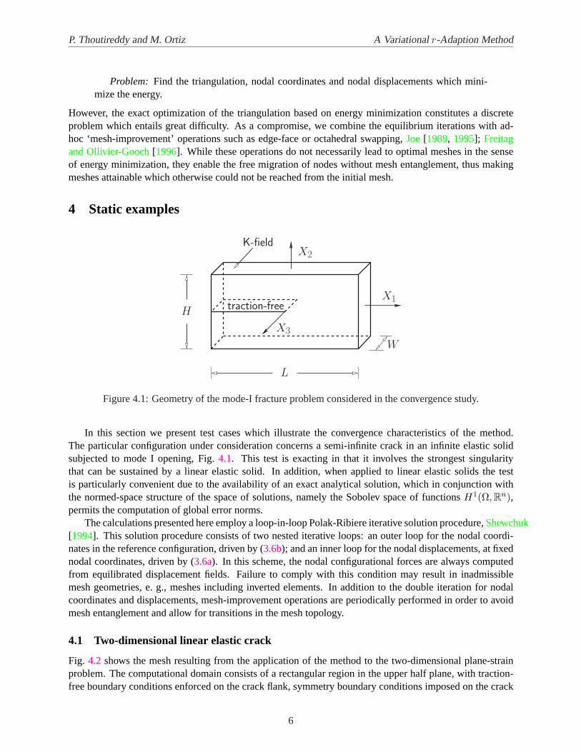
Figure 4.1:Geometry of the mode-I fracture problem considered in the convergence study.

In this section we present test cases which illustrate the convergence characteristics of the method.The particular configuration under consideration concerns a semi-infinite crack in an infinite elastic solidsubjected to mode I opening, Fig.4.1. This test is exacting in that it involves the strongest singularitythat can be sustained by a linear elastic solid. In addition, when applied to linear elastic solids the testis particularly convenient due to the availability of an exact analytical solution, which in conjunction withthe normed-space structure of the space of solutions, namely the Sobolev space of functionsH1(Ω,Rn),permits the computation of global error norms.

The calculations presented here employ a loop-in-loop Polak-Ribiere iterative solution procedure,Shewchuk[1994]. This solution procedure consists of two nested iterative loops: an outer loop for the nodal coordi-nates in the reference configuration, driven by (3.6b); and an inner loop for the nodal displacements, at fixednodal coordinates, driven by (3.6a). In this scheme, the nodal configurational forces are always computedfrom equilibrated displacement fields. Failure to comply with this condition may result in inadmissiblemesh geometries, e. g., meshes including inverted elements. In addition to the double iteration for nodalcoordinates and displacements, mesh-improvement operations are periodically performed in order to avoidmesh entanglement and allow for transitions in the mesh topology.

4.1 Two-dimensional linear elastic crack

Fig. 4.2 shows the mesh resulting from the application of the method to the two-dimensional plane-strainproblem. The computational domain consists of a rectangular region in the upper half plane, with traction-free boundary conditions enforced on the crack flank, symmetry boundary conditions imposed on the crack

6


(a) (b)

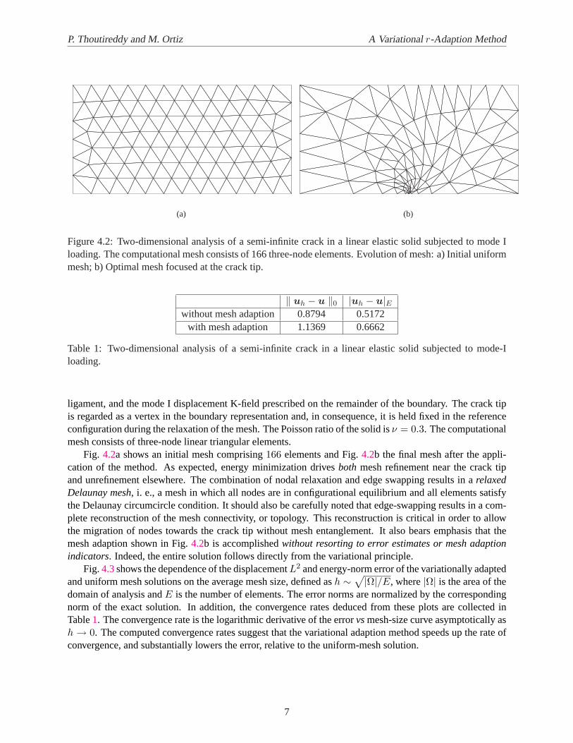
Figure 4.2:Two-dimensional analysis of a semi-infinite crack in a linear elastic solid subjected to mode Iloading. The computational mesh consists of 166 three-node elements. Evolution of mesh: a) Initial uniformmesh; b) Optimal mesh focused at the crack tip.

‖ uh − u ‖0 |uh − u|Ewithout mesh adaption 0.8794 0.5172

with mesh adaption 1.1369 0.6662

Table 1: Two-dimensional analysis of a semi-infinite crack in a linear elastic solid subjected to mode-Iloading.

ligament, and the mode I displacement K-field prescribed on the remainder of the boundary. The crack tipis regarded as a vertex in the boundary representation and, in consequence, it is held fixed in the referenceconfiguration during the relaxation of the mesh. The Poisson ratio of the solid isν = 0.3. The computationalmesh consists of three-node linear triangular elements.

Fig. 4.2a shows an initial mesh comprising166 elements and Fig.4.2b the final mesh after the appli-cation of the method. As expected, energy minimization drivesboth mesh refinement near the crack tipand unrefinement elsewhere. The combination of nodal relaxation and edge swapping results in arelaxedDelaunay mesh, i. e., a mesh in which all nodes are in configurational equilibrium and all elements satisfythe Delaunay circumcircle condition. It should also be carefully noted that edge-swapping results in a com-plete reconstruction of the mesh connectivity, or topology. This reconstruction is critical in order to allowthe migration of nodes towards the crack tip without mesh entanglement. It also bears emphasis that themesh adaption shown in Fig.4.2b is accomplishedwithout resorting to error estimates or mesh adaptionindicators. Indeed, the entire solution follows directly from the variational principle.

Fig.4.3shows the dependence of the displacementL2 and energy-norm error of the variationally adaptedand uniform mesh solutions on the average mesh size, defined ash ∼

√|Ω|/E, where|Ω| is the area of the

domain of analysis andE is the number of elements. The error norms are normalized by the correspondingnorm of the exact solution. In addition, the convergence rates deduced from these plots are collected inTable1. The convergence rate is the logarithmic derivative of the errorvsmesh-size curve asymptotically ash → 0. The computed convergence rates suggest that the variational adaption method speeds up the rate ofconvergence, and substantially lowers the error, relative to the uniform-mesh solution.

7


h

||u h

-u|

| 0

0.05 0.1 0.15 0.2 0.25 0.3

0.02

0.04

0.06

0.08

without mesh adaptionwith mesh adaption

(a)

h

|uh

-u|

E

0.05 0.1 0.15 0.2 0.25 0.3

0.1

0.2

0.3

0.4

0.5

0.6


(b)

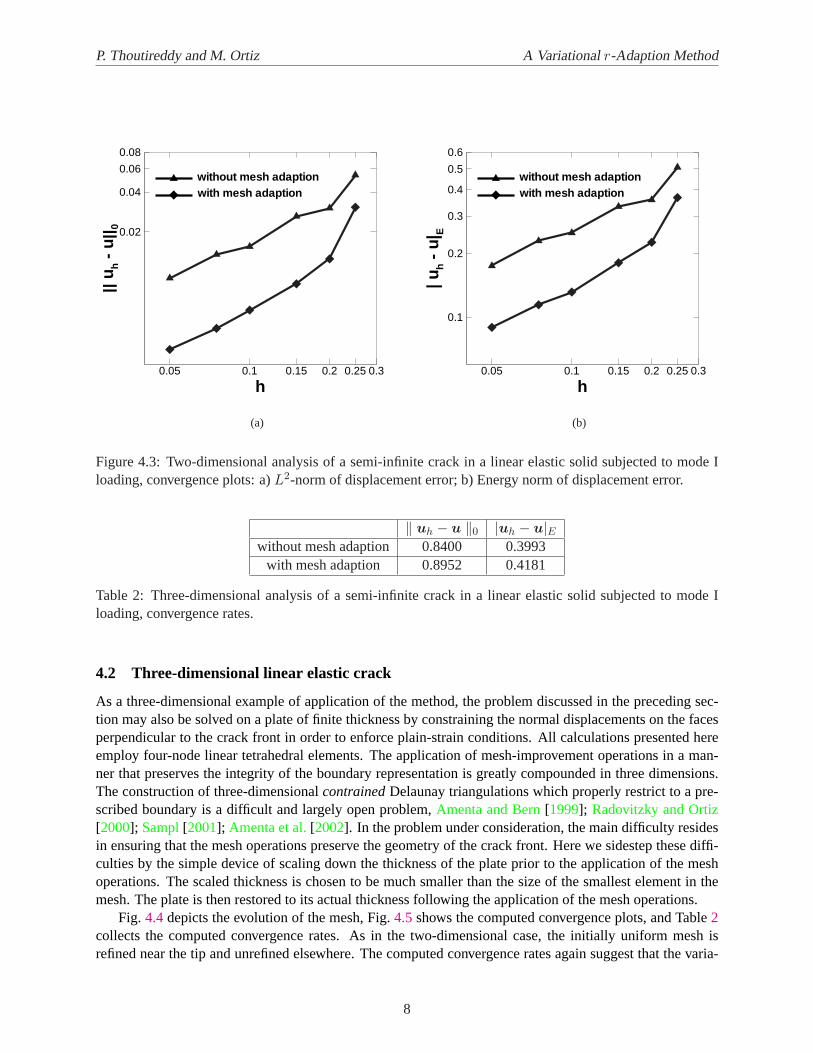
Figure 4.3:Two-dimensional analysis of a semi-infinite crack in a linear elastic solid subjected to mode Iloading, convergence plots: a)L2-norm of displacement error; b) Energy norm of displacement error.

‖ uh − u ‖0 |uh − u|Ewithout mesh adaption 0.8400 0.3993

with mesh adaption 0.8952 0.4181

Table 2: Three-dimensional analysis of a semi-infinite crack in a linear elastic solid subjected to mode Iloading, convergence rates.

4.2 Three-dimensional linear elastic crack

As a three-dimensional example of application of the method, the problem discussed in the preceding sec-tion may also be solved on a plate of finite thickness by constraining the normal displacements on the facesperpendicular to the crack front in order to enforce plain-strain conditions. All calculations presented hereemploy four-node linear tetrahedral elements. The application of mesh-improvement operations in a man-ner that preserves the integrity of the boundary representation is greatly compounded in three dimensions.The construction of three-dimensionalcontrainedDelaunay triangulations which properly restrict to a pre-scribed boundary is a difficult and largely open problem,Amenta and Bern[1999]; Radovitzky and Ortiz[2000]; Sampl[2001]; Amenta et al.[2002]. In the problem under consideration, the main difficulty residesin ensuring that the mesh operations preserve the geometry of the crack front. Here we sidestep these diffi-culties by the simple device of scaling down the thickness of the plate prior to the application of the meshoperations. The scaled thickness is chosen to be much smaller than the size of the smallest element in themesh. The plate is then restored to its actual thickness following the application of the mesh operations.

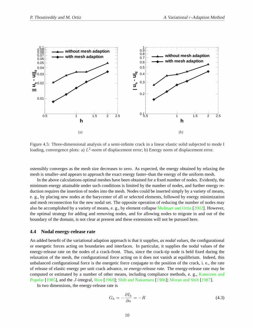
Fig. 4.4depicts the evolution of the mesh, Fig.4.5shows the computed convergence plots, and Table2collects the computed convergence rates. As in the two-dimensional case, the initially uniform mesh isrefined near the tip and unrefined elsewhere. The computed convergence rates again suggest that the varia-

8


(a) (b)

Figure 4.4:Three-dimensional analysis of a semi-infinite crack in a linear elastic solid subjected to mode Iloading. The computational mesh consists of 493 three-node elements. Evolution of mesh: a) Initial uniformmesh; b) Optimal mesh focused at the crack tip.

tional adaption method speeds up the rate of convergence, and substantially lowers the error, relative to theuniform-mesh solution.

4.3 Two-dimensional crack in a neo-Hookean solid

Next we demonstrate the applicability of the method to nonlinear problems by revisiting the problem pre-sented in Section4.1 and considering a crack in a compressible neo-Hookean solid characterized by thestrain-energy density

W (F ) =12λ0 log2(J)− µ0 log(J) +

µ0

2tr(F T F ) (4.1)

whereλ0 and µ0 are material constants andJ = det(F ) is the Jacobian of the deformation. For thismaterial, the first Piola-Kirchhoff stress follows as

P = λ0 log(J)F−T + µ0(F − F−T ) (4.2)

The material constants used in calculations areλ0 = 1.255× 108 andµ0 = 8.365× 107, corresponding toan undeformed Young’s modulusE0 = 2.175× 108 and Poisson’s rationν0 = 0.3.

Fig. 4.6a shows an initial uniform mesh comprising 166 elements, and Fig.4.6b the final mesh after theapplication of the variational adaption method. As before, energy minimization drives both mesh refinementnear the crack tip and coarsening elsewhere. As argued in the introduction, owing to the finite kinematicsinvolved in this problem, there is no natural norm that provides a measure of the numerical error, and conver-gence should be understood directly in terms of the energy of the system. Fig.4.7shows the dependence ofthe energy, computed with and without adaption, on the mesh size. As is evident from the figure, the energy

9


h

||u h

-u|

| 0

0.5 1 1.5 2 2.5

0.01

0.02

0.03

0.040.050.060.070.080.09

0.1without mesh adaptionwith mesh adaption

(a)

h

|uh

-u|

E

0.5 1 1.5 2 2.50.1

0.2

0.3

0.4

0.5

0.60.70.80.9

1


(b)

Figure 4.5:Three-dimensional analysis of a semi-infinite crack in a linear elastic solid subjected to mode Iloading, convergence plots: a)L2-norm of displacement error; b) Energy norm of displacement error.

ostensibly converges as the mesh size decreases to zero. As expected, the energy obtained by relaxing themesh is smaller–and appears to approach the exact energy faster–than the energy of the uniform mesh.

In the above calculations optimal meshes have been obtained for a fixed number of nodes. Evidently, theminimum energy attainable under such conditions is limited by the number of nodes, and further energy re-duction requires the insertion of nodes into the mesh. Nodes could be inserted simply by a variety of means,e. g., by placing new nodes at the barycenter of all or selected elements, followed by energy minimizationand mesh reconnection for the new nodal set. The opposite operation of reducing the number of nodes mayalso be accomplished by a variety of means, e. g., by element collapseMolinari and Ortiz[2002]. However,the optimal strategy for adding and removing nodes, and for allowing nodes to migrate in and out of theboundary of the domain, is not clear at present and these extensions will not be pursued here.

4.4 Nodal energy-release rate

An added benefit of the variational adaption approach is that it supplies,as nodal values, the configurationalor energetic forces acting on boundaries and interfaces. In particular, it supplies the nodal values of theenergy-release rate on the nodes of a crack-front. Thus, since the crack-tip node is held fixed during therelaxation of the mesh, the configurational force acting on it does not vanish at equilibrium. Indeed, thisunbalanced configurational force is the energetic force conjugate to the position of the crack, i. e., the rateof release of elastic energy per unit crack advance, orenergy-release rate. The energy-release rate may becomputed or estimated by a number of other means, including compliance methods, e. g.,Kanninen andPopelar[1985], and theJ-integral,Rice[1968]; Shih and Nakamura[1986]; Moran and Shih[1987].

In two dimensions, the energy-release rate is

Gh = −∂Ih

∂a= −R (4.3)

10


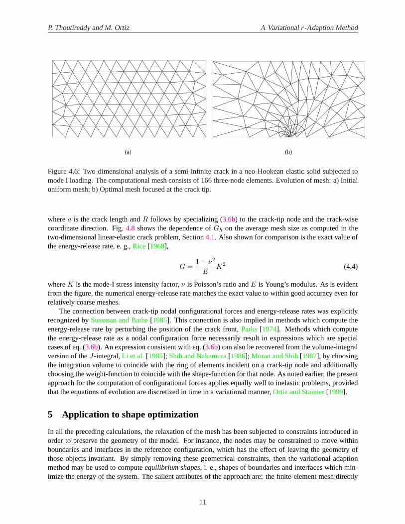
(a) (b)

Figure 4.6:Two-dimensional analysis of a semi-infinite crack in a neo-Hookean elastic solid subjected tomode I loading. The computational mesh consists of 166 three-node elements. Evolution of mesh: a) Initialuniform mesh; b) Optimal mesh focused at the crack tip.

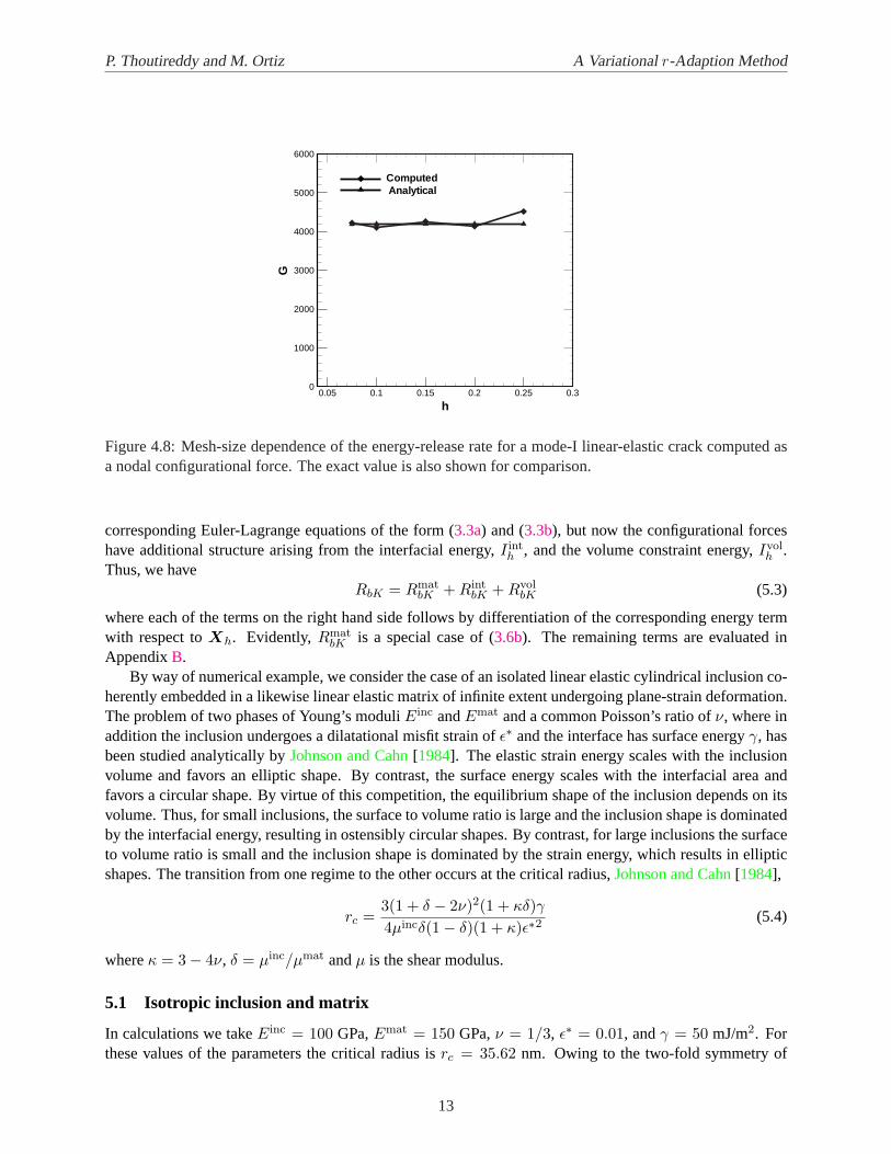
wherea is the crack length andR follows by specializing (3.6b) to the crack-tip node and the crack-wisecoordinate direction. Fig.4.8 shows the dependence ofGh on the average mesh size as computed in thetwo-dimensional linear-elastic crack problem, Section4.1. Also shown for comparison is the exact value ofthe energy-release rate, e. g.,Rice[1968],

G =1− ν2

EK2 (4.4)

whereK is the mode-I stress intensity factor,ν is Poisson’s ratio andE is Young’s modulus. As is evidentfrom the figure, the numerical energy-release rate matches the exact value to within good accuracy even forrelatively coarse meshes.

The connection between crack-tip nodal configurational forces and energy-release rates was explicitlyrecognized bySussman and Bathe[1985]. This connection is also implied in methods which compute theenergy-release rate by perturbing the position of the crack front,Parks[1974]. Methods which computethe energy-release rate as a nodal configuration force necessarily result in expressions which are specialcases of eq. (3.6b). An expression consistent with eq. (3.6b) can also be recovered from the volume-integralversion of theJ-integral,Li et al. [1985]; Shih and Nakamura[1986]; Moran and Shih[1987], by choosingthe integration volume to coincide with the ring of elements incident on a crack-tip node and additionallychoosing the weight-function to coincide with the shape-function for that node. As noted earlier, the presentapproach for the computation of configurational forces applies equally well to inelastic problems, providedthat the equations of evolution are discretized in time in a variational manner,Ortiz and Stainier[1999].

5 Application to shape optimization

In all the preceding calculations, the relaxation of the mesh has been subjected to constraints introduced inorder to preserve the geometry of the model. For instance, the nodes may be constrained to move withinboundaries and interfaces in the reference configuration, which has the effect of leaving the geometry ofthose objects invariant. By simply removing these geometrical constraints, then the variational adaptionmethod may be used to computeequilibrium shapes, i. e., shapes of boundaries and interfaces which min-imize the energy of the system. The salient attributes of the approach are: the finite-element mesh directly

11


h

I h

0 0.1 0.2 0.32000

2100

2200

2300

2400

2500

2600

2700

2800

2900

3000


Figure 4.7:Two-dimensional analysis of a semi-infinite crack in a neo-Hookean elastic solid subjected tomode I loading. Energyvsmesh size for uniform and relaxed meshes.

supplies the geometrical representation of the system; the equilibration of configurational forces optimizesthe mesh and the geometry of the system simultaneously; and the approach allows for arbitrary materialbehavior, including anisotropy and nonlinearity.

By way of illustration we specifically consider the problem of determining the equilibrium shape of anelastic inclusion, e. g., a second-phase particle or a precipitate, embedded in a likewise elastic matrix. Ouraim here is merely to illustrate how the variational adaption method can be applied to problems of shapeoptimization. A comprehensive study of the mechanics of symmetry-breaking transitions or the behaviorof specific materials is beyond the scope of this work and may be found elsewhere (see, e. g.,Voorhees[1985]; Voorhees et al.[1988]; Voorhees[1992]; Voorhees et al.[1992]; Jou et al.[1997]; Leo et al.[2000,2001], and references therein). Alternative approaches to shape optimization may also be found elsewhere(e. g.,Maute and Ramm[1995, 1997]; Bendsoe and Kikuchi[1988]; Leo et al.[1998]; Maute et al.[1999];Schleupen et al.[2000]; Jog et al.[2000]; Hou et al.[2001]; Schwarz et al.[2001]).

A simple form of the energy of the inclusion/matrix system is

I =∫

BW (Gradϕ)dV +

∫

ΓγdS +

α

2

(V2 −

∫

B2

dV

)2

(5.1)

whereB2 is domain of the precipitate,B1 = B − B2 the domain of the matrix,Γ is the interface betweenthe precipitate and the matrix,γ is the interface energy density for interface,V2 volume of the precipitate,andα a penalty parameter. For simplicity we take the interfacial energy to be isotropic. Upon discretization,the energy function is

Ih =∫

BW (Gradϕh)dV +

∫

ΓγdS +

α

2

(V2 −

∫

B2

dV

)2

≡ Imath + I int

h + Ivolh (5.2)

which, as before, is to be regarded as a function of the nodal coordinatesxh andXh in the deformed andundeformed configurations, respectively. The equilibrium shape of the precipitate now follows by mini-mization of Ih with respect toxh,Xh. The stationarity condition is again of the form (3.2), and the

12


h

G

0.05 0.1 0.15 0.2 0.25 0.30

1000

2000

3000

4000

5000

6000

ComputedAnalytical

Figure 4.8:Mesh-size dependence of the energy-release rate for a mode-I linear-elastic crack computed asa nodal configurational force. The exact value is also shown for comparison.

corresponding Euler-Lagrange equations of the form (3.3a) and (3.3b), but now the configurational forceshave additional structure arising from the interfacial energy,I int

h , and the volume constraint energy,Ivolh .

Thus, we haveRbK = Rmat

bK + RintbK + Rvol

bK (5.3)

where each of the terms on the right hand side follows by differentiation of the corresponding energy termwith respect toXh. Evidently, Rmat

bK is a special case of (3.6b). The remaining terms are evaluated inAppendixB.

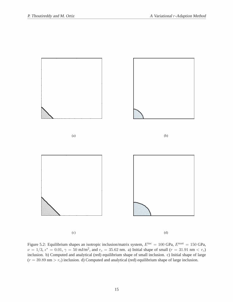
By way of numerical example, we consider the case of an isolated linear elastic cylindrical inclusion co-herently embedded in a likewise linear elastic matrix of infinite extent undergoing plane-strain deformation.The problem of two phases of Young’s moduliEinc andEmat and a common Poisson’s ratio ofν, where inaddition the inclusion undergoes a dilatational misfit strain ofε∗ and the interface has surface energyγ, hasbeen studied analytically byJohnson and Cahn[1984]. The elastic strain energy scales with the inclusionvolume and favors an elliptic shape. By contrast, the surface energy scales with the interfacial area andfavors a circular shape. By virtue of this competition, the equilibrium shape of the inclusion depends on itsvolume. Thus, for small inclusions, the surface to volume ratio is large and the inclusion shape is dominatedby the interfacial energy, resulting in ostensibly circular shapes. By contrast, for large inclusions the surfaceto volume ratio is small and the inclusion shape is dominated by the strain energy, which results in ellipticshapes. The transition from one regime to the other occurs at the critical radius,Johnson and Cahn[1984],

rc =3(1 + δ − 2ν)2(1 + κδ)γ4µincδ(1− δ)(1 + κ)ε∗2

(5.4)

whereκ = 3− 4ν, δ = µinc/µmat andµ is the shear modulus.

5.1 Isotropic inclusion and matrix

In calculations we takeEinc = 100 GPa,Emat = 150 GPa,ν = 1/3, ε∗ = 0.01, andγ = 50 mJ/m2. Forthese values of the parameters the critical radius isrc = 35.62 nm. Owing to the two-fold symmetry of

13


Figure 5.1:Initial inclusion shape and finite-element mesh adopted in the computation of the equilibriumshapes of inclusions.

the system the computational domain may be reduced to one single quadrant. The initial mesh used in thecalculations is shown in Fig.5.1and consists of linear triangular elements.

The computed equilibrium shapes for inclusions of sizesr = 31.91 nm < rc, andr = 39.89 nm > rc,are shown in Fig.5.2, which also displays the analytical equilibrium shapes for comparison,Johnson andCahn[1984]. As is evident from the figure, the computed equilibrium shapes are in close agreement with thecorresponding analytical solutions. In particular, the small inclusion adopts a spherical shape at equilibrium,whereas the large inclusion adopts an elliptical shape, in keeping with the stability analysis ofJohnson andCahn[1984].

5.2 Cubic inclusion and matrix

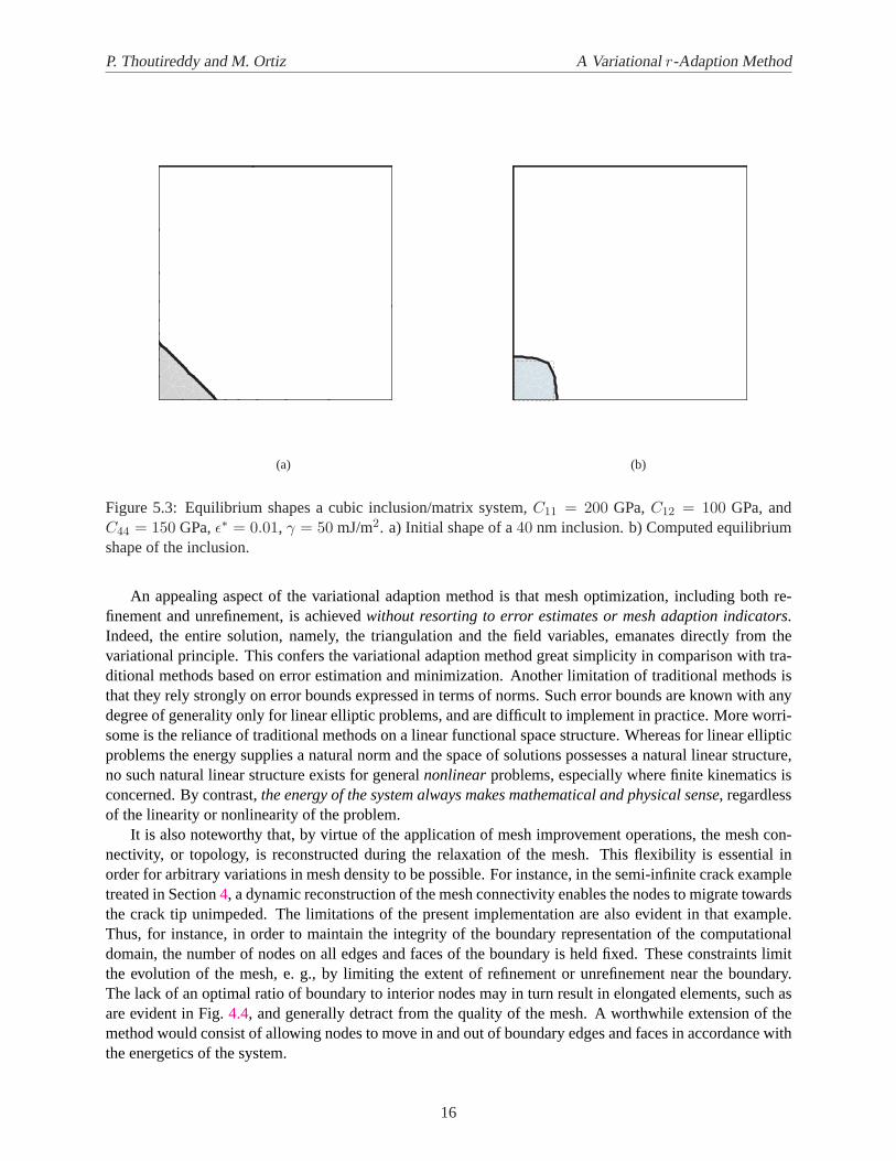
Next we consider cubic phases of elastic moduliC11 = 200 GPa,C12 = 100 GPa, andC44 = 150GPa, a misfit strainε∗ = 0.01 in the inclusion, a surface energyγ = 50 mJ/m2, and an inclusion size of40nm. Fig.5.3 shows the computed equilibrium shape of the inclusion, which is closer to a square shapethan in the isotropic case. Although no analytical solution appears to be in existence for this problem, thecomputed equilibrium shape is in close agreement with those computed by other methods byJog et al.[2000], Thomson and Voorhees[1994], andSchmidt and Gross[1997].

6 Conclusions

We have developed a variationalr-adaption method for static problems. The distinguishing characteristicof this method is that it relies on the variational principle to simultaneously supply the solution, the optimalmesh and, in problems of shape optimization, the equilibrium shapes of the system. This is accomplishedby minimizing the energy functional with respect to the nodal field values as well as with respect to thetriangulation of the domain of analysis. Energy minimization with respect to the field variables has theeffect of equilibrating the body, whereas energy minimization with respect to the referential nodal positionshas the effect of equilibrating the energetic orconfigurational forcesacting on the nodes.

14


(a) (b)

(c) (d)

Figure 5.2:Equilibrium shapes an isotropic inclusion/matrix system,Einc = 100 GPa,Emat = 150 GPa,ν = 1/3, ε∗ = 0.01, γ = 50 mJ/m2, andrc = 35.62 nm. a) Initial shape of small (r = 31.91 nm < rc)inclusion. b) Computed and analytical (red) equilibrium shape of small inclusion. c) Initial shape of large(r = 39.89 nm> rc) inclusion. d) Computed and analytical (red) equilibrium shape of large inclusion.

15


(a) (b)

Figure 5.3:Equilibrium shapes a cubic inclusion/matrix system,C11 = 200 GPa,C12 = 100 GPa, andC44 = 150 GPa,ε∗ = 0.01, γ = 50 mJ/m2. a) Initial shape of a40 nm inclusion. b) Computed equilibriumshape of the inclusion.

An appealing aspect of the variational adaption method is that mesh optimization, including both re-finement and unrefinement, is achievedwithout resorting to error estimates or mesh adaption indicators.Indeed, the entire solution, namely, the triangulation and the field variables, emanates directly from thevariational principle. This confers the variational adaption method great simplicity in comparison with tra-ditional methods based on error estimation and minimization. Another limitation of traditional methods isthat they rely strongly on error bounds expressed in terms of norms. Such error bounds are known with anydegree of generality only for linear elliptic problems, and are difficult to implement in practice. More worri-some is the reliance of traditional methods on a linear functional space structure. Whereas for linear ellipticproblems the energy supplies a natural norm and the space of solutions possesses a natural linear structure,no such natural linear structure exists for generalnonlinearproblems, especially where finite kinematics isconcerned. By contrast,the energy of the system always makes mathematical and physical sense, regardlessof the linearity or nonlinearity of the problem.

It is also noteworthy that, by virtue of the application of mesh improvement operations, the mesh con-nectivity, or topology, is reconstructed during the relaxation of the mesh. This flexibility is essential inorder for arbitrary variations in mesh density to be possible. For instance, in the semi-infinite crack exampletreated in Section4, a dynamic reconstruction of the mesh connectivity enables the nodes to migrate towardsthe crack tip unimpeded. The limitations of the present implementation are also evident in that example.Thus, for instance, in order to maintain the integrity of the boundary representation of the computationaldomain, the number of nodes on all edges and faces of the boundary is held fixed. These constraints limitthe evolution of the mesh, e. g., by limiting the extent of refinement or unrefinement near the boundary.The lack of an optimal ratio of boundary to interior nodes may in turn result in elongated elements, such asare evident in Fig.4.4, and generally detract from the quality of the mesh. A worthwhile extension of themethod would consist of allowing nodes to move in and out of boundary edges and faces in accordance withthe energetics of the system.

16


Acknowledgements

Support from the DoE through Caltech’s ASCI/ASAP Center for the Simulation of the Dynamic Responseof Solids, and from the ONR grant number NOOO14-96-1-0068, is gratefully acknowledged.

A Configurational forces for isoparametric elements

In this appendix we derive explicit expressions for the nodal configurational forces for isoparametric ele-ments. Begin by expressing the discrete energy in the form

Ih =E∑

e=1

∫

Ωe

W (Gradϕh)dV −∫

Ωe

RB ·ϕhdV −∫

∂Ωe∩∂B2

T ·ϕhdS

≡ I

(1)h − I

(2)h − I

(3)h (A.1)

whereE is the number of elements andΩe is the undeformed domain of elemente. Next we computethe variations of each of the terms in Eq.A.1 with respect toXh, for the particular case of isoparametricinterpolation, i. e., for local shape functions of the form

N ea = Na ηe−1 (A.2)

where

ηe(X) =n∑

a=1

XeaNa(X) (A.3)

is the isoparametric mapping for elemente, defined over the standard domainΩ of the element, andXea are

the nodal coordinates in the undeformed configuration of the element. Begin by writing

I(1)h =

E∑

e=1

∫

ΩW

(n∑

a=1

xiaNa,A∂XA

∂XJ

)det(∇ηe)dΩ (A.4)

Taking variations with respect toδXh gives:

δI(1)h =

E∑

e=1

∫

Ω

−PiJ

[n∑

a=1

xiaNa,A∂XA

∂XK

(n∑

b=1

δXebKNb,B

)∂XB

∂XJ

]

+W

(n∑

b=1

δXebKNb,B

)∂XB

∂XK

det(∇ηe)dΩ

(A.5)

or

δI(1)h =

E∑

e=1

∫

Ωe

MJK

(n∑

b=1

δXebKNb,J

)dV (A.6)

whereMJK = WδJK − FiKPiJ (A.7)

is Eshelby’s energy-momentum tensor,Eshelby[1975]. In addition we have

I(2)h =

E∑

e=1

∫

ΩRBi

(n∑

a=1

xiaNa

)det(∇ηe)dΩ (A.8)

17


Taking variations we obtain

δI(2)h =

E∑

e=1

∫

ΩRBi

(n∑

a=1

xiaNa

)(n∑

b=1

δXebKNb,B

)∂XB

∂XKdet(∇ηe)dΩ (A.9)

or

δI(2)h =

E∑

e=1

∫

ΩRBiϕi

(n∑

b=1

δXebKNb,K

)dV (A.10)

Finally we turn to the traction term. To this end, letP be any tensor-valued function such thatPiJNJ = Ti

on∂B2 andPiJNJ = 0 on∂B1. In practice, the functionP need only be one element deep. Then we have

I(3)h =

∫

∂BPiJNJϕidS =

∫

B(PiJϕi),J dV =

∫

B(PiJϕi,J + PiJ,Jϕ)dV (A.11)

Each of the two term in the last expression can now be given a treatment identical to the termsI(1)h andI

(2)h

discussed earlier. Collecting all terms we obtain

δIh =E∑

e=1

∫

Ωe

[W − Pk,Lϕk,L − (RBk − PkL,L)ϕk]δJK − (PiJ − PiJ)FiK

(

n∑

b=1

δXebKNb,J

)dV

(A.12)Collecting terms, the nodal configurational force follows as

RKb =∂Ih

∂XKb=

E∑

e=1

∫

Ωe

MKJ + [−Pk,Lϕk,L − (RBk − PkL,L)ϕk]δJK + PiJFiK

Nb,JdV (A.13)

B Configurational forces for interface optimization

In optimizing the shape of elastic inclusions the energy needs to be augmented by the addition of interfa-cial and volume constraint terms. For simplicity, we consider the case of constant and isotropic surfaceenergy, and finite elements whose restrictions to the interfaces to be optimized define a collection of surfaceisoparametric elementsΓe, e = 1, . . . , S. Thus, for every elemente, the isoparametric mapping

X = ηe(X1, X2) (B.1)

maps the standard domainΓ into the actual domainΓe of the element inR3. Here(X1, X2) are parametriccoordinates defined onΓ. Under these assumptions, the interfacial energy takes the form

I inth =

S∑

e=1

∫

Γγ |ηe

,1 × ηe,2| dΓ (B.2)

Taking variations we obtain

δI inth =

S∑

e=1

∫

Γγ

(ηe,1 × ηe

,2)I

|ηe,1 × ηe

,2|εIKM

(n∑

b=1

[(ηe

,2)M Nb,1 − (ηe,1)M Nb,2

]δXe

bK

)dΓ (B.3)

whence it follows that

RintbK =

S∑

e=1

∫

Γγ

(ηe,1 × ηe

,2)I

|ηe,1 × ηe

,2|εIKM

[(ηe

,2)M Nb,1 − (ηe,1)M Nb,2

]dΓ (B.4)

18


Likewise, taking variations of the volume constraint we obtain

δIvolh = −α

(V2 −

∫

B2

dV

) E2∑

e=1

∫

Ωe

(n∑

b=1

δXebKN e

b,K

)dV (B.5)

whereE2 is the number of elements inB2. From this identity we obtain

RvolbK = −α

(V2 −

∫

B2

dV

) E2∑

e=1

∫

Ωe

N eb,K dV (B.6)

References

N. Amenta and M. Bern. Surface reconstruction by voronoi filtering.Discrete & Computational Geometry, 22(4):481–504, 1999.

N. Amenta, S. Choi, T.K. Dey, and N. Leekha. A simple algorithm for homeomorphic surface reconstruction.Inter-national Journal of Computational Geometry & Applications, 12(1-2):125–141, 2002.

M.P. Bendsoe and N. Kikuchi. Generating optimal topologies in structural design using a homogenization method.Computer Methods in Applied Mechanics and Engineering, 71(2):197–224, 1988.

J.D. Eshelby. The elastic energy-momentum tensor.Journal of Elasticity, 5(3-4):321–335, 1975.

L.C. Evans.Partial Differential Equations. American Mathematical Society, Providence, Rhode Island, 1998.

L Freitag and C. Ollivier-Gooch. A comparison of tetrahedral mesh improvement techniques. InProceedings of the5th International Meshing Roundtable, pages 87–100, Pittsburgh, Pennsylvania, October 1996. Sandia NationalLaboratories.

M.E. Gurtin. The nature of configurational forces.Archive for Rational Mechanics and Analysis, 131:67–100, 1995.

M.E. Gurtin.Configurational Forces as Basic Concepts of Continuum Physics. Springer-Verlag Inc., New York, 2000.

C. M. Hoffmann.Geometric and Solid Modeling. Morgan Kaufmann Publishers, San Mateo, California, 1989.

T.Y. Hou, J.S. Lowengrub, and M.J. Shelley. Boundary integral methods for multicomponent fluids and multiphasematerials.Journal of Computational Physics, 169(2):302–362, 2001.

B. Joe. Three-dimensional triangulations from local transformations.SIAM Journal on Scientific and StatisticalComputing, 10:718–741, 1989.

B. Joe. Construction of three-dimensional improved-quality triangulations using local transformations.SIAM Journalon Scientific Computing, 16(6):1292–1307, November 1995.

C.S. Jog, R. Sankarasubramanian, and T.A. Abinandanan. Symmetry-breaking transitions in equilibrium shapes ofcoherent precipitates.Journal of the mechanics and Physics of Solids, 48(11):2363–2389, 2000.

W.C. Johnson and J.W. Cahn. Elastically induced shape bifurcations of inclusions.Acta Metallurgica, 32((11)), 1984.

H.J. Jou, P.H. Leo, and J.S. Lowengrub. Microstructural evolution in inhomogeneous elastic media.Journal ofComputational Physics, 131(1):109–148, 1997.

M.F. Kanninen and C.H. Popelar.Advanced Fracture Mechanics. Oxford University Press, 1985.

P.H. Leo, J.S. Lowengrub, and H.J. Jou. A diffuse interface model for microstructural evolution in elastically stressedsolids.Acta Materialia, 46(6):2113–2130, 1998.

19


P.H. Leo, J.S. Lowengrub, and Q. Nie. Microstructural evolution in orthotropic elastic media.Journal of Computa-tional Physics, 157(1):44–88, 2000.

P.H. Leo, J.S. Lowengrub, and Q. Nie. On an elastically induced splitting instability.Acta Materialia, 49(14):2761–2772, 2001.

F. Z. Li, C. F. Shih, and A. Needleman. A Comparison of Methods for Calculating Energy Release Rates.EngineeringFracture Mechanics, 21:405–421, 1985.

M. Mantyla. An Introduction to Solid Modeling. Computer Science Press, Rockwille, Maryland, 1988.

K. Maute and E. Ramm. Adaptive topology optimization.Structural Optimization, 10(2):100–112, 1995.

K. Maute and E. Ramm. Adaptive topology optimization of shell structures.AIAA Journal, 35(11):1767–1773, 1997.

K. Maute, S. Schwarz, and E. Ramm. Structural optimization - the interaction between form and mechanics.Zeitschriftfur Angewandte Mathematik und Mechanik, 79(10):651–673, 1999.

J.F. Molinari and M. Ortiz. Three-dimensional adaptive meshing by subdivision and edge-collapse in finite-deformation dynamic- plasticity problems with application to adiabatic shear banding.International Journal forNumerical Methods in Engineering, 53(5):1101–1126, 2002.

B. Moran and C. F. Shih. A general treatment of crack tip contour integrals.International Journal of Fracture, 35:295–310, 1987.

M. Ortiz and L. Stainier. The variational formulation of viscoplastic constitutive updates.Computer Methods inApplied Mechanics and Engineering, 171(3-4):419–444, 1999.

D. M. Parks. A Stiffness Derivative Finite Element Technique for Determination of Crack-Tip Stress Intensity Factors.International Journal of Fracture, 10:487–502, 1974.

R. Radovitzky and M. Ortiz. Error estimation and adaptive meshing in strongly nonlinear dynamic problems.Com-puter Methods in Applied Mechanics and Engineering, 172(1-4):203–240, 1999.

R. Radovitzky and M. Ortiz. Tetrahedral mesh generation based on node insertion in crystal lattice arrangements andadvancing-front-Delaunay triangulation.Computer Methods in Applied Mechanics and Engineering, 187:543–569,2000.

A. A. G. Requicha. Representations for rigid solids: Theory, methods and systems.Computing Surveys, 12:437–465,1980.

J.R. Rice. A path independent integral and the approximate analysis of strain concentration by notches and cracks.Journal of Applied Mechanics, 35:379–386, 1968.

P. Sampl. Medial axis construction in three dimensions and its application to mesh generation.Engineering withComputers, 17(3):234–248, 2001.

A. Schleupen, K. Maute, and E. Ramm. Adaptive fe-procedures in shape optimization.Structural and Multidisci-plinary Optimization, 19(4):282–302, 2000.

I. Schmidt and D. Gross. The equilibrium shape of an elastically inhomogeneous inclusion.Journal of the Mechanicsand Physics of Solids, 45:1521–1549, 1997.

S. Schwarz, K. Maute, and E. Ramm. Topology and shape optimization for elastoplastic structural response.ComputerMethods in Applied Mechanics and Engineering, 190(15-17):2135–2155, 2001.

J. R. S. Shewchuk. An introduction to the conjugate gradient method without agonizing pain. Technical report,University of California, Berkeley, http://www.cs.berkeley.edu/ jrs, 1994.

20


Moran B. Shih, C. F. and T. Nakamura. Energy release rate along a three dimensional crack front in a thermallystressed body.International Journal of Fracture, 30:79–102, 1986.

G. Strang and G. J. Fix.An Analysis of the Finite Element Method. Prentice-Hall, Englewood Cliffs, N.J., 1973.

T. Sussman and K.J. Bathe. The gradient of the finite element variational indicator with respect to nodal point co-ordinates: An explicit calculation and applications in fracture mechanics and mesh optimization.InternationalJournal for Numerical Methods in Engineering, 21:763–774, 1985.

Su C.S. Thomson, M.E. and P.W. Voorhees. The equilibrium shape of a misfitting precipitate.Acta Metallurgica etMaterialia, 42:2107–2122, 1994.

P.W. Voorhees. The theory of ostwald ripening.Journal of Statistical Physics, 38(1-2):231–252, 1985.

P.W. Voorhees. Ostwald ripening of 2-phase mixtures.Annual Review of Materials Science, 22:197–215, 1992.

P.W. Voorhees, G.B. McFadden, R.F. Boisvert, and D.I. Meiron. Numerical-simulation of morphological developmentduring ostwald ripening.Acta Metallurgica, 36(1):207–222, 1988.

P.W. Voorhees, G.B. McFadden, and W.C. Johnson. On the morphological development of 2nd-phase particles inelastically-stressed solids.Acta Metallurgica et Materialia, 40(11):2979–2992, 1992.

21

A Variational r-Adaption and Shape-Optimization Method for Finite-Deformation...

Documents

Transcript of A Variational r-Adaption and Shape-Optimization Method for Finite-Deformation...