A Variational Inequality from Pricing Convertible Bond · A Variational Inequality from Pricing ......
21
Hindawi Publishing Corporation Advances in Difference Equations Volume 2011, Article ID 309678, 21 pages doi:10.1155/2011/309678 Research Article A Variational Inequality from Pricing Convertible Bond Huiwen Yan and Fahuai Yi School of Mathematics, South China Normal University, Guangzhou 510631, China Correspondence should be addressed to Fahuai Yi, [email protected] Received 30 December 2010; Accepted 11 February 2011 Academic Editor: Jin Liang Copyright q 2011 H. Yan and F. Yi. This is an open access article distributed under the Creative Commons Attribution License, which permits unrestricted use, distribution, and reproduction in any medium, provided the original work is properly cited. The model of pricing American-style convertible bond is formulated as a zero-sum Dynkin game, which can be transformed into a parabolic variational inequality PVI. The fundamental variable in this model is the stock price of the firm which issued the bond, and the differential operator in PVI is linear. The optimal call and conversion strategies correspond to the free boundaries of PVI. Some properties of the free boundaries are studied in this paper. We show that the bondholder should convert the bond if and only if the price of the stock is equal to a fixed value, and the firm should call the bond back if and only if the price is equal to a strictly decreasing function of time. Moreover, we prove that the free boundaries are smooth and bounded. Eventually we give some numerical results. 1. Introduction Firms raise capital by issuing debt bonds and equity shares of stock. The convertible bond is intermediate between these two instruments, which entitles its owner to receive coupons plus the returnof principle at maturity. However, prior to maturity, the holder may convert the bond into the stock of the firm, surrendering it for a preset number of shares of stock. On the other hand, prior to maturity, the firm may call the bond forcing the bondholder to either surrender it to the firm for a previously agreed price or convert it into stock as before. After issuing a convertible bond, the bondholder will find a proper time to exercise the conversion option in order to maximize the value of the bond, and the firm will choose its optimal time to exercise its call option to maximize the value of shareholder’s equity. This situation was called “two-person” game see 1, 2. Because the firm must pay coupons to the bondholder, it may call the bond if it can subsequently reissue a bond with a lower coupon rate. This happens as the firm’s fortunes improve, then the risk of default has diminished and investors will accept a lower coupon rate on the firm’s bonds.
-
Upload
hoangkhanh -
Category
Documents
-
view
218 -
download
0
Transcript of A Variational Inequality from Pricing Convertible Bond · A Variational Inequality from Pricing ......
Hindawi Publishing CorporationAdvances in Difference EquationsVolume 2011, Article ID 309678, 21 pagesdoi:10.1155/2011/309678
Research ArticleA Variational Inequality from PricingConvertible Bond
Huiwen Yan and Fahuai Yi
School of Mathematics, South China Normal University, Guangzhou 510631, China
Correspondence should be addressed to Fahuai Yi, [email protected]
Received 30 December 2010; Accepted 11 February 2011
Academic Editor: Jin Liang
Copyright q 2011 H. Yan and F. Yi. This is an open access article distributed under the CreativeCommons Attribution License, which permits unrestricted use, distribution, and reproduction inany medium, provided the original work is properly cited.
The model of pricing American-style convertible bond is formulated as a zero-sum Dynkin game,which can be transformed into a parabolic variational inequality (PVI). The fundamental variablein this model is the stock price of the firm which issued the bond, and the differential operator inPVI is linear. The optimal call and conversion strategies correspond to the free boundaries of PVI.Some properties of the free boundaries are studied in this paper. We show that the bondholdershould convert the bond if and only if the price of the stock is equal to a fixed value, and the firmshould call the bond back if and only if the price is equal to a strictly decreasing function of time.Moreover, we prove that the free boundaries are smooth and bounded. Eventually we give somenumerical results.
1. Introduction
Firms raise capital by issuing debt (bonds) and equity (shares of stock). The convertible bondis intermediate between these two instruments, which entitles its owner to receive couponsplus the return of principle at maturity. However, prior to maturity, the holder may convertthe bond into the stock of the firm, surrendering it for a preset number of shares of stock. Onthe other hand, prior to maturity, the firm may call the bond forcing the bondholder to eithersurrender it to the firm for a previously agreed price or convert it into stock as before.
After issuing a convertible bond, the bondholder will find a proper time to exercisethe conversion option in order to maximize the value of the bond, and the firm will chooseits optimal time to exercise its call option to maximize the value of shareholder’s equity. Thissituation was called “two-person” game (see [1, 2]). Because the firm must pay coupons tothe bondholder, it may call the bond if it can subsequently reissue a bondwith a lower couponrate. This happens as the firm’s fortunes improve, then the risk of default has diminished andinvestors will accept a lower coupon rate on the firm’s bonds.
2 Advances in Difference Equations
In [2] the authors assume that a firm’s value is comprised of one equity and oneconvertible bond, the value of the issuing firm has constant volatility, the bond continuouslypays coupons at a fixed rate, and the firm continuously pays dividends at a rate that is a fixedfraction of equity. Default occurs if the coupon payments cause the firm’s value to fall to zero,in which case the bond has zero value. In their model, both the bond price and the stock priceare functions of the underlying of the firm value. Because the stock price is the differencebetween firm value and bond price and dividends are paid proportionally to the stock price,a nonlinear differential equation was established for describing the bond price as a functionof the firm value and time.
As we know, it is difficult to obtain the value of the firm. However, it is easier to get itsstock price. So we choose the bond price V (S, t) as a function of the stock price S of the firmand time t (see Chapter 36 in [3] or [4–7]).
In Section 2, we formulate the model and deduce that V (S, t) = γS in the domain{S ≥ K/γ} and V (S, t) is governed by the following variational inequality in the domain{0 ≤ S ≤ K/γ}:
−∂tV − L0V = c, if V < K, (S, t) ∈ DTΔ=(0,
K
γ
)× [0, T),
−∂tV − L0V ≤ c, if V = K, (S, t) ∈ DT,
V
(K
γ, t
)= K, 0 ≤ t ≤ T,
V (S, T) = max{L, γS
}, 0 ≤ S ≤ K
γ,
(1.1)
where c, γ , K, and L are positive constants. c is the coupon rate, γ is the conversion ratio forconverting the bond into the stock of the firm,K is the call price of the firm, L is the face valueof the bond with 0 < L ≤ K, and L0 is just B-S operator (see [8]),
L0V =σ2
2S2∂SSV +
(r − q
)S∂SV − rV, (1.2)
where r, σ, and q are positive constants and represent the risk-free interest rate, the volatility,and the dividend rate of the firm stock, respectively. In this paper, we suppose that c > rKand r ≥ q. From a financial point of view, the assumption provides a possibility of callingthe bond back from the firm (see Section 2 or [2]). Furthermore, we suppose that L ≤ K.Otherwise, the firm should call the bond back before maturity and the value L makes nosense (see Section 2). It is clear that V = K is the unique solution if L = K. So we onlyconsider the problem in the case of L < K.
Since (1.1) is a degenerate backward problem, we transform it into a familiar forwardnondegenerate parabolic variational inequality problem; so letting
u(x, t) = V (S, T − t), x = lnS − lnK + ln γ, (1.3)
Advances in Difference Equations 3
we have that
∂tu − Lu = c, if u < K, (x, t) ∈ ΩTΔ= (−∞, 0) × (0, T],
∂tu − Lu ≤ c, if u = K, (x, t) ∈ ΩT ,
u(0, t) = K, 0 ≤ t ≤ T,
u(x, 0) = max{L,Kex}, x ≤ 0,
(1.4)
where
Lu =σ2
2∂xxu +
(r − q − σ2
2
)∂xu − ru. (1.5)
There are many papers on the convertible bond, such as [1, 2, 9]. But as we know, thereare seldom results on the properties of the free boundaries—the optimal call and conversionstrategies in the existing literature. The main aim of this paper is to analyze some propertiesof the free boundaries.
The pricing model of the convertible bond without call is considered in [9], wherethere exist two domains: the continuation domain CT and the conversion domain CV. Thefree boundary S(t) between CT and CV means the optimal conversion strategy, which isdependent on the time t and more than K/γ .
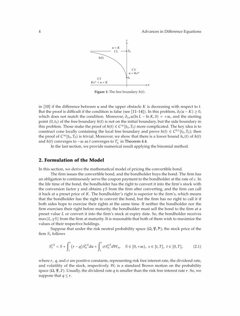
But in this model, their exist three domains: the continuation domain CT, thecallable domain CL, and the conversion domain CV = {x ≥ 0}. The boundary between CVand CT ∪ CL is x = 0, which means the call strategy. The free boundary h(t) is the curvebetween CT and CL (see Figure 1), which means the optimal call strategy. And there existt0, T0 such that
0 < t0 < T0Δ=1rln
c − rL
c − rK, h(t) ∈ C[t0, T0) ∩ C∞[t0, T0), lim
t→T−0
h(t) = −∞, (1.6)
and h(t) is strictly decreasing in [t0, T0).It means that the bondholder should convert the bond if and only if the stock price
S of the firm is no less than K/γ , whereas, in the model without call, the bondholder maynot convert the bond even if S > K/γ . More precisely, the optimal conversion strategy S(t)without call is more than that K/γ in this paper (see [9] or Section 2). When the time tothe expiry date is more than T0, the firm should call the bond back if S < K/γ . Neither thebondholder nor the firm should exercise their option if the time to the expiry date is less thant0 and S < Keh(t). Moreover, when the time to the maturity lies in (t0, T0), the bondholdershould call the bond back ifKeh(t) ≤ S < K/γ .
In Section 2, we formulate and simplify the model. In Section 3, we will prove theexistence and uniqueness of the strong solution of the parabolic variational inequality (1.4)and establish some estimations, which are important to analyze the property of the freeboundary.
In Section 4, we show some behaviors of the free boundary h(t), such as its startingpoint and monotonicity. Particularly, we obtain the regularity of the free boundary h(t) ∈C0,1[t0, T0) ∩ C∞[t0, T0). As we know, the proof of the smoothness is trivial by the method
4 Advances in Difference Equations
t
x
t0
T0u = K
CTKex < u < K
CL
u = KexCV
h(t)
Figure 1: The free boundary h(t).
in [10] if the difference between u and the upper obstacle K is decreasing with respect to t.But the proof is difficult if the condition is false (see [11–14]). In this problem, ∂t(u −K) ≥ 0,which does not match the condition. Moreover, ∂xxu(lnL − lnK, 0) = +∞, and the startingpoint (0, t0) of the free boundary h(t) is not on the initial boundary, but the side boundary inthis problem. Those make the proof of h(t) ∈ C∞[t0, T0) more complicated. The key idea is toconstruct cone locally containing the local free boundary and prove h(t) ∈ C0,1[t0, T0); thenthe proof of C∞[t0, T0) is trivial. Moreover, we show that there is a lower bound h∗(t) of h(t)and h(t) converges to −∞ as t converges to T−
0 in Theorem 4.4.In the last section, we provide numerical result applying the binomial method.
2. Formulation of the Model
In this section, we derive the mathematical model of pricing the convertible bond.The firm issues the convertible bond, and the bondholder buys the bond. The firm has
an obligation to continuously serve the coupon payment to the bondholder at the rate of c. Inthe life time of the bond, the bondholder has the right to convert it into the firm’s stock withthe conversion factor γ and obtains γS from the firm after converting, and the firm can callit back at a preset price of K. The bondholder’s right is superior to the firm’s, which meansthat the bondholder has the right to convert the bond, but the firm has no right to call it ifboth sides hope to exercise their rights at the same time. If neither the bondholder nor thefirm exercises their right before maturity, the bondholder must sell the bond to the firm at apreset value L or convert it into the firm’s stock at expiry date. So, the bondholder receivesmax{L, γS} from the firm at maturity. It is reasonable that both of them wish to maximize thevalues of their respective holdings.
Suppose that under the risk neutral probability space (Ω,F,�); the stock price of thefirm Ss follows
St,Ss = S +
∫ s
t
(r − q
)St,Su du +
∫ s
t
σSt,Su dWu, S ∈ [0,+∞), s ∈ [t, T], t ∈ [0, T], (2.1)
where r, q, and σ are positive constants, representing risk free interest rate, the dividend rate,and volatility of the stock, respectively. Wt is a standard Brown motion on the probabilityspace (Ω,F,�). Usually, the dividend rate q is smaller than the risk free interest rate r. So, wesuppose that q ≤ r.
Advances in Difference Equations 5
Denote by Ft the natural filtration generated by Wt and augmented by all the �-nullsets in F. Let Ut,T be the set of all Ft-stopping times taking values in [t, T].
Themodel can be expressed as a zero-sumDynkin game. The payoff of the bondholderis
R(S, t; τ, θ) =∫ τ∧θ
t
cert−rudu + ert−rτKI{τ<θ} + ert−rθγSt,Sθ I{θ≤τ, θ<T}
+ ert−rT max{L, γSt,S
T
}I{τ∧θ=T},
(2.2)
where τ, θ ∈ Ut,T . The stopping time τ is the firm’s strategy, and θ is the bondholder’s strategy.The bondholder chooses his strategy θ to maximize R(S, t; τ, θ); meanwhile, the firm
chooses its strategy τ to minimize R(S, t; τ, θ).Denote the upper value V and the lower value V as
V (S, t) Δ= ess supθ∈Ut,T
ess infτ∈Ut,T
�[R(S, t; τ, θ) | Ft],
V (S, t) Δ= ess infτ∈Ut,T
ess supθ∈Ut,T
�[R(S, t; τ, θ) | Ft].(2.3)
If V (S, t) = V (S, t), then it is called the value of the Dynkin game and denoted as V (S, t).As we know, if the Dynkin game has a saddlepoint (τ∗, θ∗) ∈ Ut,T × Ut,T , that is,
�[R(S, t; τ∗, θ) | Ft] ≤ �[R(S, t; τ∗, θ∗) | Ft] ≤ �[R(S, t; τ, θ∗) | Ft], ∀τ, θ ∈ Ut,T , (2.4)
then the value of the Dynkin game exists and
V (S, t) = �[R(S, t; τ∗, θ∗) | Ft]. (2.5)
If S ≥ K/γ , then we deduce that, for any τ, θ ∈ Ut,T ,
�[R(S, t; τ, t) | Ft] = γSI{t<T} +max{L, γS
}I{t=T} = �[R(S, t; t, t) | Ft],
�[R(S, t; t, θ) | Ft] = �[KI{t<θ} + γSI{θ=t} | Ft
]I{t<T} +max
{L, γS
}I{t=T} ≤ �[R(S, t; t, t) | Ft].
(2.6)
So, in this case, (t, t) is a saddlepoint, and the value of the Dynkin game is
V (S, t) = γSI{t<T} +max{L, γS
}I{t=T}, ∀S ≥ K
γ. (2.7)
6 Advances in Difference Equations
In the case of 0 < S < K/γ , applying the standard method in [15], we see that thestrong solution of the following variational inequality is the value of the Dynkin game:
−∂tV − L0V = c, if γS < V < K, (S, t) ∈ DT,
−∂tV − L0V ≥ c, if V = γS, (S, t) ∈ DT,
−∂tV − L0V ≤ c, if V = K, (S, t) ∈ DT,
V
(K
γ, t
)= K, 0 ≤ t ≤ T,
V (S, T) = max{L, γS
}, 0 ≤ S ≤ K
γ.
(2.8)
If L > K, then the firm is bound to call the bond back before the maturity because the firmpaysK after calling, but more than Lwithout calling. In this case, the value Lmakes no sense.So, we suppose that L ≤ K.
If c ≤ rK, then the firm is bound to abandon its call right. From a financial point ofview, the firm would payK to the bondholder at time t after calling the bond, whereas, if thefirm does not call in the time interval [t, t + dt], then he would pay the coupon payment cdtand at mostK of the face value of the convertible bond at time t+dt. So, the discounted valueof the bond without call is at most K + cdt − rKdt ≤ K. Hence, the firm should not call thebond back at time t.
From a stochastic point of view, we can denote a stopping time
τ1 = inf{t ≤ u ≤ T : γSt,S
u ≥ K}. (2.9)
If t < T , 0 < S < K/γ , then �(τ1 > t) = 1, and, for any θ ∈ Ut,T , we have
R(S, t; τ1, θ) =c
r+ I{τ1<θ}e
rt−rτ1(K − c
r
)+ I{θ≤τ1,θ<T}e
rt−rθ(γSt,S
θ − c
r
)
+ I{τ1∧θ=T}ert−rT
(max
{L, γSt,S
T
}− c
r
)
≤ c
r+ ert−r(τ1∧θ∧T)
(K − c
r
)= K ≤ R(S, t; t, θ) a.s. in Ω.
(2.10)
Moreover, �(R(S, t; τ1, θ) < R(S, t; t, θ)) = 1. So, for any τ, θ ∈ Ut,T such that �(τ = t) > 0, it isclear that in the domain {t < T, 0 < S < K/γ}
�[R(S, t; τ, θ) | Ft] > �[R(S, t; τI{τ>t} + τ1I{τ=t}, θ
) | Ft
], (2.11)
which means that τ is not the optimal call strategy, and the firm should not call in the domain{t < T, 0 < S < K/γ}.
Advances in Difference Equations 7
From a variational inequality point of view, since
−∂tK − L0K = rK > c, (2.12)
provided that c < rK, which contradicts with the third inequality in (2.8), so, if c < rK, thenV /=K in the domain {t < T, 0 < S < Kγ}.
To remain the call strategy, we suppose that c > rK. We will consider the other case inanother paper because the two problems are fully different.
Since we suppose that c > rK and r ≥ q, then
−∂t(γS
) − L0(γS
)= qγS ≤ rK < c. (2.13)
Hence, {V = γS} is empty in problem (2.8). So, problem (2.8) is reduced into problem (1.1).The model of pricing the bond without call is an optimal stopping problem
U(S, t) Δ= ess supθ∈Ut,T
�[Q(S, t; θ) | Ft],
Q(S, t; θ) =∫θ
t
cert−rudu + ert−rθγSt,SθI{θ<T} + ert−rT max
{L, γSt,S
T
}I{θ=T}.
(2.14)
It is clear that
U(S, t) = ess supθ∈Ut,T
�[R(S, t; T, θ) | Ft] ≥ V (S, t). (2.15)
Since U,V ≥ γS, then
{U = γS
} ⊂ {V = γS
}, CV∗ ⊂ CV, (2.16)
where CV∗ is the conversion domain in the model without call and CV is that in this paper.
3. The Existence and Uniqueness of W2,1p,loc Solution of Problem (1.4)
Since problem (1.4) lies in the unbounded domain ΩT , we need the following problem in the
bounded domain ΩnT
Δ= (−n, 0) × (0, T] to approximate to problem (1.4):
∂tun − Lun = c, if un < K, (x, t) ∈ ΩnT ,
∂tun − Lun ≤ c, if un = K, (x, t) ∈ ΩnT ,
un(−n, t) = L, un(0, t) = K, 0 ≤ t ≤ T,
un(x, 0) = max{L,Kex}, −n ≤ x ≤ 0,
(3.1)
where n ∈ IN+ and n > lnK − lnL.
8 Advances in Difference Equations
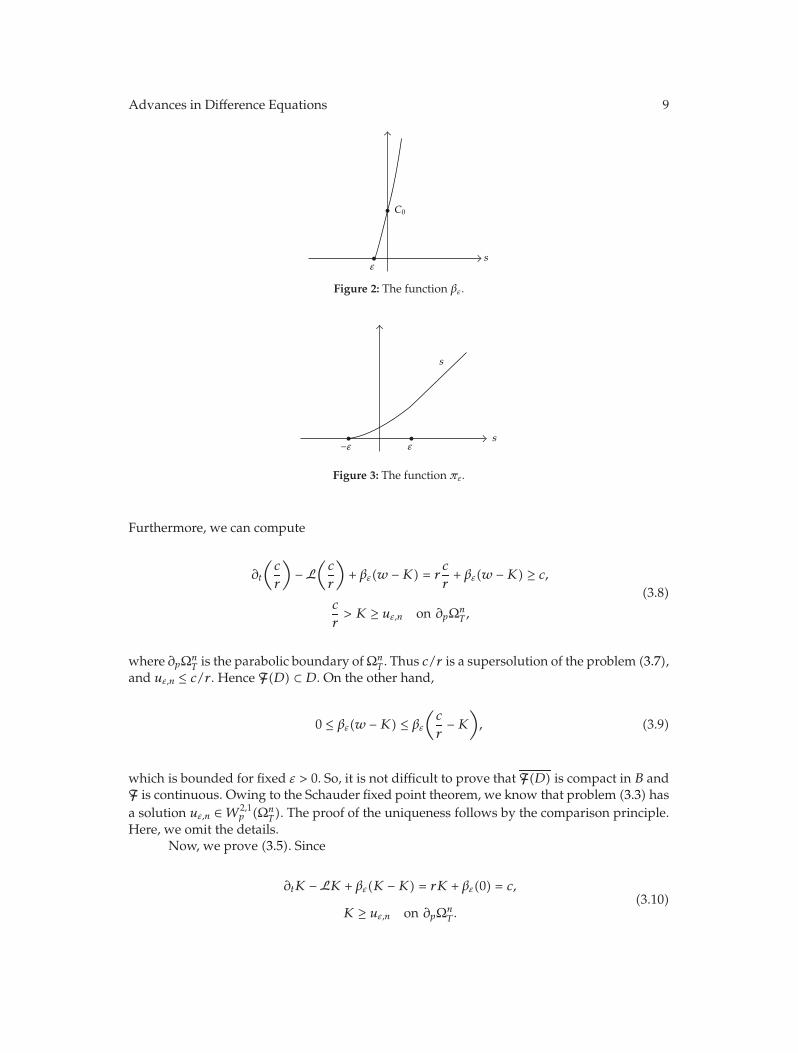
Following the idea in [10, 16], we construct a penalty function βε(s) (see Figure 2),which satisfies
ε > 0 and small enough, βε(s) ∈ C∞(−∞,+∞),
βε(s) = 0, if s ≤ −ε, βε(0) = C0Δ= c − rK > 0,
βε(s) ≥ 0, β′ε(s) ≥ 0, β′′ε(s) ≥ 0,
limε→ 0
βε(s) =
⎧⎨⎩0, s < 0,
+∞, s > 0.
(3.2)
Consider the following penalty problem of (3.1):
∂tuε,n − Luε,n + βε(uε,n −K) = c, in ΩnT ,
uε,n(−n, t) = L, uε,n(0, t) = K, 0 ≤ t ≤ T,
uε,n(x, 0) = πε(Kex − L) + L, −n ≤ x ≤ 0,
(3.3)
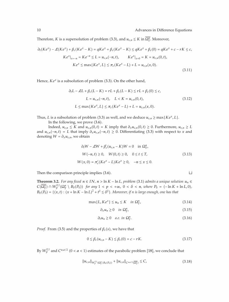
where πε(s) is a smoothing function because the initial value max{L,Kex} is not smooth. Itsatisfies (see Figure 3)
πε(s) =
⎧⎨⎩s, s ≥ ε,
0, s ≤ −ε,
πε(s) ∈ C∞(IR), πε(s) ≥ s, 0 ≤ π ′ε(s) ≤ 1, π ′′
ε (s) ≥ 0, limε→ 0+
πε(s) = s+.
(3.4)
Lemma 3.1. For any fixed ε > 0, problem (3.3) has a unique solution uε,n ∈ W2,1p (Ωn
T ) ∩ C(ΩnT ) for
any 1 < p < +∞ and
max{L,Kex} ≤ uε,n ≤ K in ΩnT , (3.5)
∂xuε,n ≥ 0 in ΩnT . (3.6)
Proof. We apply the Schauder fixed point theorem [17] to prove the existence of nonlinearproblem (3.3).
Denote B = C(ΩnT ) and D = {w ∈ B : w ≤ c/r}. Then D is a closed convex set in B.
Defining a mapping F by F(w) = uε,n is the solution of the following linear problem:
∂tuε,n − Luε,n + βε(w −K) = c in ΩnT ,
uε,n(−n, t) = L, uε,n(0, t) = K, 0 ≤ t ≤ T,
uε,n(x, 0) = πε(Kex − L) + L, −n ≤ x ≤ 0.
(3.7)
Advances in Difference Equations 9
ε
C0
s
Figure 2: The function βε.
s
s−ε ε
Figure 3: The function πε.
Furthermore, we can compute
∂t
(c
r
)− L
(c
r
)+ βε(w −K) = r
c
r+ βε(w −K) ≥ c,
c
r> K ≥ uε,n on ∂pΩn
T ,
(3.8)
where ∂pΩnT is the parabolic boundary ofΩn
T . Thus c/r is a supersolution of the problem (3.7),and uε,n ≤ c/r. Hence F(D) ⊂ D. On the other hand,
0 ≤ βε(w −K) ≤ βε
(c
r−K
), (3.9)
which is bounded for fixed ε > 0. So, it is not difficult to prove that F(D) is compact in B andF is continuous. Owing to the Schauder fixed point theorem, we know that problem (3.3) hasa solution uε,n ∈ W2,1
p (ΩnT ). The proof of the uniqueness follows by the comparison principle.
Here, we omit the details.Now, we prove (3.5). Since
∂tK − LK + βε(K −K) = rK + βε(0) = c,
K ≥ uε,n on ∂pΩnT .
(3.10)
10 Advances in Difference Equations
Therefore,K is a supersolution of problem (3.3), and uε,n ≤ K in ΩnT . Moreover,
∂t(Kex) − L(Kex) + βε(Kex −K) = qKex + βε(Kex −K) ≤ qKex + βε(0) = qKex + c − rK ≤ c,
Kex|x=−n = Ke−n ≤ L = uε,n(−n, t), Kex|x=0 = K = uε,n(0, t),
Kex ≤ max{Kex, L} ≤ πε(Kex − L) + L = uε,n(x, 0).(3.11)
Hence, Kex is a subsolution of problem (3.3). On the other hand,
∂tL − LL + βε(L −K) = rL + βε(L −K) ≤ rL + βε(0) ≤ c,
L = uε,n(−n, t), L < K = uε,n(0, t),
L ≤ max{Kex, L} ≤ πε(Kex − L) + L = uε,n(x, 0).
(3.12)
Thus, L is a subsolution of problem (3.3) as well, and we deduce uε,n ≥ max{Kex, L}.In the following, we prove (3.6).Indeed, uε,n ≤ K and uε,n(0, t) = K imply that ∂xuε,n(0, t) ≥ 0. Furthermore, uε,n ≥ L
and uε,n(−n, t) = L that imply ∂xuε,n(−n, t) ≥ 0. Differentiating (3.3) with respect to x anddenoting W = ∂xuε,n, we obtain
∂tW − LW + β′ε(uε,n −K)W = 0 in ΩnT ,
W(−n, t) ≥ 0, W(0, t) ≥ 0, 0 ≤ t ≤ T,
W(x, 0) = π ′ε(Kex − L)Kex ≥ 0, −n ≤ x ≤ 0.
(3.13)
Then the comparison principle implies (3.6).
Theorem 3.2. For any fixed n ∈ IN, n > lnK − lnL, problem (3.1) admits a unique solution un ∈C(Ωn
T ) ∩ W2,1p (Ωn
T \ Bδ(P0)) for any 1 < p < +∞, 0 < δ < n, where P0 = (− lnK + lnL, 0),Bδ(P0) = {(x, t) : (x + lnK − lnL)2 + t2 ≤ δ2}. Moreover, if n is large enough, one has that
max{L,Kex} ≤ un ≤ K in ΩnT , (3.14)
∂xun ≥ 0 in ΩnT , (3.15)
∂tun ≥ 0 a.e. in ΩnT . (3.16)
Proof. From (3.5) and the properties of βε(s), we have that
0 ≤ βε(uε,n −K) ≤ βε(0) = c − rK. (3.17)
By W2,1p and Cα,α/2 (0 < α < 1) estimates of the parabolic problem [18], we conclude that
‖uε,n‖W2,1p (Ωn
T\Bδ(P0)) + ‖uε,n‖Cα,α/2(ΩnT )≤ C, (3.18)
Advances in Difference Equations 11
where C is independent of ε. It implies that there exists a un ∈ W2,1p (Ωn
T \Bδ(P0))∩C(ΩnT ) and
a subsequence of {uε,n} (still denoted by {uε,n}), such that as ε → 0+,
uε,n ⇀ un in W2,1p
(Ωn
T \ Bδ(P0))weakly, uε,n −→ un in C
(Ωn
T
). (3.19)
Employing the method in [16] or [19], it is not difficult to derive that un is the solutionof problem (3.1). And (3.14), (3.15) are the consequence of (3.5), (3.6) as ε → 0+.
In the following, we will prove (3.16). For any small δ > 0, w(x, t) Δ= un(x, t + δ)satisfies, by (3.1),
∂tw − Lw = c, if w < K, (x, t) ∈ (−n, 0) × (0, T − δ],
∂tw − Lw ≤ c, if w = K, (x, t) ∈ (−n, 0) × (0, T − δ],
w(−n, t) = L = un(−n, t), w(0, δ) = K = un(0, t), 0 ≤ t ≤ T − δ,
w(x, 0) = un(x, δ) ≥ max{L,Kex} = un(x, 0), −n ≤ x ≤ 0.
(3.20)
Applying the comparison principle with respect to the initial value of the variationalinequality (see [16]), we obtain
un(x, t + δ) = w(x, t) ≥ un(x, t), (x, t) ∈ (−n, 0) × (0, T − δ]. (3.21)
Thus (3.16) follows.At last, we prove the uniqueness of the solution. Suppose that u1
n and u2n are two
W2,1p,loc(Ω
nT ) ∩C(Ωn
T ) solutions to problem (3.1), and denote
N Δ={(x, t) ∈ Ωn
T : u1n(x, t) < u2
n(x, t)}. (3.22)
Assume that N is not empty, and then, in the domainN,
u1n(x, t) < u2
n(x, t) ≤ K, ∂tu1n − Lu1
n = c, ∂t(u1n − u2
n
)− L
(u1n − u2
n
)≥ 0. (3.23)
Denoting W = u1n − u2
n, we have that
∂tW − LW ≥ 0 in N, W = 0 on ∂pN. (3.24)
Applying the A-B-P maximum principle (see [20]), we have that W ≥ 0 in N, whichcontradicts the definition of N.
12 Advances in Difference Equations
Theorem 3.3. Problem (1.4) has a unique solution u ∈ C(ΩT)∩W2,1p (ΩR
T \Bδ(P0)) for any 1 < p <
+∞, R > 0, and δ > 0. And ∂xu ∈ C(ΩT \ Bδ(P0)). Moreover,
max{L,Kex} ≤ u ≤ K in ΩT , (3.25)
∂xu ≥ 0 a.e. in ΩT , (3.26)
∂tu ≥ 0 a.e. in ΩT . (3.27)
Proof. Rewrite Problem (3.1) as follows:
∂tun − Lun = f(x, t), (x, t) ∈ ΩnT ,
un(−n, t) = L, un(0, t) = K, 0 ≤ t ≤ T,
un(x, 0) = max{L,Kex}, −n ≤ x ≤ 0,
(3.28)
where un ∈ W2,1p (Ωn
T \ Bδ(P0)) implies that f(x, t) ∈ Lp
loc(ΩnT ) and
f(x, t) = cI{un<K} + rKI{un=K}, (3.29)
where IA denotes the indicator function of the set A.Hence, for any fixed R > δ > 0, if n > R, combining (3.14), we have the following W2,1
p
and Cα,α/2 uniform estimates [18]:
‖un‖W2,1p (ΩR
T \Bδ(P0)) ≤ CR,δ, ‖un‖Cα,α/2(ΩR
T )≤ CR, (3.30)
here CR,δ depends on R and δ, CR depends on R, but they are independent of n. Then, wehave that there is a u ∈ W2,1
p,loc(ΩT )∩C(Ω)T and a subsequence of {un} (still denoted by {un}),such that for any R > δ > 0, p > 1,
un ⇀ u in W2,1p
(ΩR
T \ Bδ(P0))weakly as n −→ +∞. (3.31)
Moreover, (3.30) and imbedding theorem imply that
un −→ u in C
(Ω
R
T
), ∂xun −→ ∂xu in C
(Ω
R
T \ Bδ(P0))
as n −→ +∞. (3.32)
It is not difficult to deduce that u is the solution of problem (1.4). Furthermore, (3.32) impliesthat ∂xu ∈ C(ΩT \ Bδ(P0)). And (3.25)–(3.27) are the consequence of (3.14)–(3.16). The proofof the uniqueness is similar to the proof in Theorem 3.2.
Advances in Difference Equations 13
4. Behaviors of the Free Boundary
Denote
CT = {(x, t) : u(x, t) < K} (continuation region
),
CL = {(x, t) : u(x, t) = K} (callable region
).
(4.1)
Thanks to (3.26), we can define the free boundary h(t) of problem (1.4), at which it isoptimal for the firm to call the bond, where
h(t) = inf{x ≤ 0 : u(x, t) = K}, 0 < t ≤ T (4.2)
(see Figure 1). It is clear that
CT = {x < h(t)}, CL = {h(t) ≤ x < 0}. (4.3)
Theorem 4.1. Denote T0 = (1/r) ln((c − rL)/(c − rK)). If t ≥ T0, then u(x, t) ≡ K, which meansthat
CT ⊂ {0 < t < T0, x < 0}, CL ⊃ {t ≥ T0, x < 0}, h(t) = −∞ for any t ≥ T0. (4.4)
Proof. Define
w(x, t) =
⎧⎪⎨⎪⎩
c
r−(c
r− L
)e−rt, 0 ≤ t ≤ T0,
K, T0 ≤ t ≤ T.(4.5)
We claim that w(x, t) possess the following four properties.
(i) w ∈ W2,1p,loc(ΩT ) ∩ C(ΩT ),
(ii) w ≤ K, for all (x, t) ∈ ΩT ,
(iii) w(x, 0) = L ≤ max{L,Kex} = u(x, 0), for all x ∈ (−∞, 0],
(iv) ∂tw − Lw ≤ c, a.e. in ΩT .
In fact, from the definition of T0, we have that
w(x, T0) =c
r−(c
r− L
)exp
{−r 1
rln
c − rL
c − rK
}= K, (4.6)
then property (i) is obvious.Moreover, if 0 < t ≤ T0, then we deduce
∂tw(x, t) = r
(c
r− L
)e−rt ≥ 0. (4.7)
14 Advances in Difference Equations
Combining w(x, T0) = K, we have property (ii). It is easy to check property (iii) fromthe definition of w. Next, we manifest property (iv) according to the following two cases. Inthe case of 0 < t ≤ T0,
∂tw − Lw = r
(c
r− L
)e−rt + r
[c
r−(c
r− L
)e−rt
]= c. (4.8)
In the other case of T0 < t ≤ T ,
∂tw − Lw = rK < c. (4.9)
So, we testify properties (i)–(iv). In the following, we utilize the properties to provew ≤ u.Otherwise, N = {w > u} is nonempty; then we have that
u(x, t) < w(x, t) ≤ K, ∂tu − Lu = c, ∂t(u −w) − L(u −w) ≥ 0, in N. (4.10)
Moreover, u − w ≥ 0 on the parabolic boundary of N. According to the A-B-P maximumprinciple (see [20]), we have that
u −w ≥ 0 in N, (4.11)
which contradicts the definition ofN. So, we achieve that w ≤ u.Combining w(x, t) = K for any t ≥ T0, it is clear that
K = w(x, t) ≤ u(x, t) ≤ K, for any t ≥ T0, (4.12)
which means that CT ⊂ {0 < t < T0, x < 0}, CL ⊃ {t ≥ T0, x < 0}, and h(t) = −∞ for anyt ≥ T0
Theorem 4.2. The free boundary h(t) is decreasing in the interval (0, T0). Moreover, h(0) Δ=limt→ 0+h(t) = 0. And h(t) ∈ C[0, T0).
Proof. (3.26) and (3.27) imply that
∂x(u −K) ≥ 0, ∂t(u −K) ≥ 0 a.e. in ΩT . (4.13)
Hence, for any unit vector n = (n1, n2) satisfying n1, n2 > 0, the directional derivativeof function u −K along n admits
∂n(u −K) ≥ 0 a.e. in ΩT , (4.14)
that is, u −K is increasing along the director n. Combining the condition u −K ≤ 0 in ΩT , weknow that x = h(t) is monotonically decreasing. Hence, limt→ 0+h(t) exists, and we can define
h(0) = limt→ 0+
h(t). (4.15)
Advances in Difference Equations 15
Since u(0, t) = K, so h(0) ≤ 0. On the other hand, if h(0) < 0, then
u(x, t) = K, ∀(x, t) ∈ (h(0), 0) × (0, T], u(x, 0) = max{L,Kex} < K, ∀x ∈ (h(0), 0).(4.16)
It is impossible because u is continuous on ΩT .In the following, we prove that h(t) is continuous in (0, T0). If it is false, then there
exists x1 < x2 < 0, 0 < t1 < T0 such that (see Figure 4)
limt→ t−1
h(t) = x1, limt→ t+1
h(t) = x2. (4.17)
Moreover,
∂tu − Lu = c in M Δ= {(x, t) : x2 < x < h(t), 0 < t ≤ t1}. (4.18)
Differentiating (4.18) with respect to x, then
∂t(∂xu) − L(∂xu) = 0 in M. (4.19)
On the other hand, ∂xu(x, t1) = 0 for any x ∈ (x1, x2) in this case, and we know that ∂xu ≥ 0by (3.26). Applying the strong maximum principle to (4.19), we obtain
∂xu(x, t) = 0, in M. (4.20)
So, we can define u(x, t) = g(t) in M. Considering u(h(t), t) = K and u ∈ C(ΩT ), we seethat u(x, t) ≡ K in M, which contradicts that u(x, t) < K for any x < h(t). Therefore h(t) ∈C[0, T0).
Theorem 4.3. There exists some t0 ∈ (0, T0) such that h(t) = 0 for any t ∈ [0, t0] and h(t) is strictlydecreasing on [t0, T0).
Proof. Define t0 = sup{t : t ≥ 0, h(t) = 0}. In the first, we prove that t0 > 0. Otherwise, h(0) = 0and h(t) < 0 for t > 0.
Recalling the initial value, we see that
∂xu(x, 0) = Kex for any x ∈ (lnL − lnK, 0], limx→ 0−
∂xu(x, 0) = K. (4.21)
Meanwhile, u(x, t) = K in the domain {(x, t) : h(t) < x < 0, 0 < t < T0} implies that ∂xu(0, t) =0 for any t > 0 (see Figure 4); then ∂xu is not continuous at the point (0, 0), which contradicts∂xu ∈ C(ΩT \ Bδ(P0)).
In the second, we prove that t0 < T0. In fact, according to Lemma 3.1, h(t) = −∞ forany t ≥ T0, hence, t0 ≤ T0. If t0 = T0, then the free boundary includes a horizontal line t =T0, x ∈ (−∞, 0). Repeating the method in the proof of Theorem 4.2, then we can obtain acontradiction. So, t0 < T0.
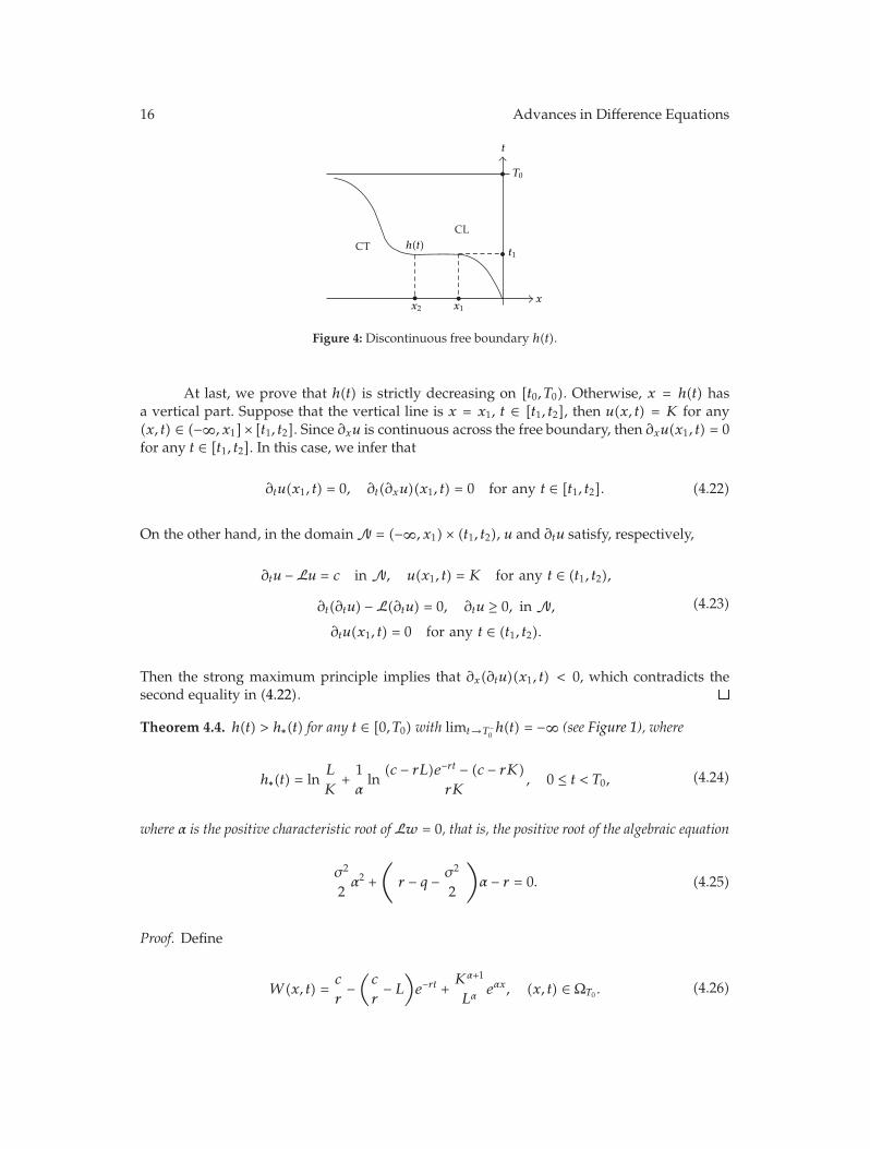
16 Advances in Difference Equations
t
xx1x2
t1
T0
CT h(t)CL
Figure 4: Discontinuous free boundary h(t).
At last, we prove that h(t) is strictly decreasing on [t0, T0). Otherwise, x = h(t) hasa vertical part. Suppose that the vertical line is x = x1, t ∈ [t1, t2], then u(x, t) = K for any(x, t) ∈ (−∞, x1]× [t1, t2]. Since ∂xu is continuous across the free boundary, then ∂xu(x1, t) = 0for any t ∈ [t1, t2]. In this case, we infer that
∂tu(x1, t) = 0, ∂t(∂xu)(x1, t) = 0 for any t ∈ [t1, t2]. (4.22)
On the other hand, in the domain N = (−∞, x1) × (t1, t2), u and ∂tu satisfy, respectively,
∂tu − Lu = c in N, u(x1, t) = K for any t ∈ (t1, t2),
∂t(∂tu) − L(∂tu) = 0, ∂tu ≥ 0, in N,
∂tu(x1, t) = 0 for any t ∈ (t1, t2).
(4.23)
Then the strong maximum principle implies that ∂x(∂tu)(x1, t) < 0, which contradicts thesecond equality in (4.22).
Theorem 4.4. h(t) > h∗(t) for any t ∈ [0, T0) with limt→ T−0h(t) = −∞ (see Figure 1), where
h∗(t) = lnL
K+1αln
(c − rL)e−rt − (c − rK)rK
, 0 ≤ t < T0, (4.24)
where α is the positive characteristic root of Lw = 0, that is, the positive root of the algebraic equation
σ2
2α2 +
(r − q − σ2
2
)α − r = 0. (4.25)
Proof. Define
W(x, t) =c
r−(c
r− L
)e−rt +
Kα+1
Lαeαx, (x, t) ∈ ΩT0 . (4.26)
Advances in Difference Equations 17
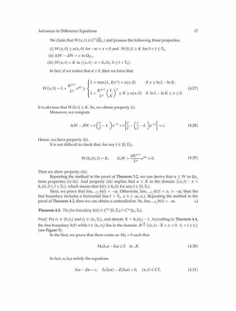
We claim that W(x, t) ∈ C2(ΩT0) and possess the following three properties.
(i) W(x, 0) ≥ u(x, 0) for −∞ < x < 0 and W(0, t) ≥ K for 0 < t ≤ T0,
(ii) ∂tW − LW = c in ΩT0 ,
(iii) W(x, t) < K in {(x, t) : x < h∗(t), 0 ≤ t < T0}.
In fact, if we notice that α > 0, then we have that
W(x, 0) = L +Kα+1
Lαeαx ≥
⎧⎪⎪⎨⎪⎪⎩L = max{L,Kex} = u(x, 0) if x ≤ lnL − lnK,
L +Kα+1
Lα
(L
K
)α
≥ K ≥ u(x, 0) if lnL − lnK ≤ x ≤ 0.(4.27)
It is obvious that W(0, t) ≥ K. So, we obtain property (i).Moreover, we compute
∂tW − LW = r
(c
r− L
)e−rt + r
[c
r−(c
r− L
)e−rt
]= c. (4.28)
Hence, we have property (ii).It is not difficult to check that, for any t ∈ [0, T0),
W(h∗(t), t) = K, ∂xW =αKα+1
Lαeαx > 0. (4.29)
Then we show property (iii).Repeating the method in the proof of Theorem 3.2, we can derive that u ≤ W in ΩT0
from properties (i)-(ii). And property (iii) implies that u < K in the domain {(x, t) : x <h∗(t), 0 ≤ t < T0}, which means that h(t) ≥ h∗(t) for any t ∈ [0, T0).
Next, we prove that limt→T−0h(t) = −∞. Otherwise, limt→ T−
0h(t) = x1 > −∞; then the
free boundary includes a horizontal line t = T0, x ∈ (−∞, x1). Repeating the method in theproof of Theorem 4.2, then we can obtain a contradiction. So, limt→ T−
0h(t) = −∞.
Theorem 4.5. The free boundary h(t) ∈ C0,1[0, T0) ∩ C∞[t0, T0).
Proof. Fix t1 ∈ (0, t0) and t2 ∈ (t0, T0), and denote X = h∗(t2) − 1. According to Theorem 4.4,
the free boundary h(t) while t ∈ (t0, t2) lies in the domain N Δ= {(x, t) : X < x < 0, t1 < t ≤ t2}(see Figure 5).
In the first, we prove that there exists anM0 > 0 such that
M0∂xu − ∂tu ≥ 0 in N. (4.30)
In fact, u, ∂tu satisfy the equations
∂tu − Lu = c, ∂t(∂tu) − L(∂tu) = 0, (x, t) ∈ CT, (4.31)
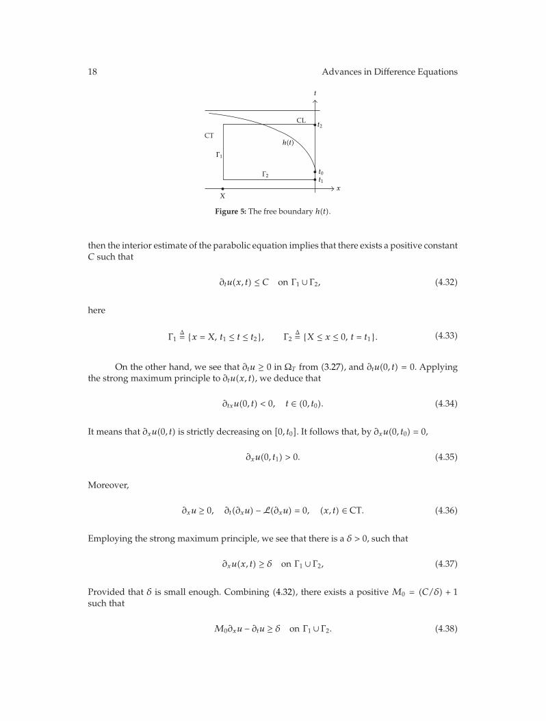
18 Advances in Difference Equations
t0t1
t2
X
CT
Γ1
Γ2
t
x
h(t)
CL
Figure 5: The free boundary h(t).
then the interior estimate of the parabolic equation implies that there exists a positive constantC such that
∂tu(x, t) ≤ C on Γ1 ∪ Γ2, (4.32)
here
Γ1Δ= {x = X, t1 ≤ t ≤ t2}, Γ2
Δ= {X ≤ x ≤ 0, t = t1}. (4.33)
On the other hand, we see that ∂tu ≥ 0 in ΩT from (3.27), and ∂tu(0, t) = 0. Applyingthe strong maximum principle to ∂tu(x, t), we deduce that
∂txu(0, t) < 0, t ∈ (0, t0). (4.34)
It means that ∂xu(0, t) is strictly decreasing on [0, t0]. It follows that, by ∂xu(0, t0) = 0,
∂xu(0, t1) > 0. (4.35)
Moreover,
∂xu ≥ 0, ∂t(∂xu) − L(∂xu) = 0, (x, t) ∈ CT. (4.36)
Employing the strong maximum principle, we see that there is a δ > 0, such that
∂xu(x, t) ≥ δ on Γ1 ∪ Γ2, (4.37)
Provided that δ is small enough. Combining (4.32), there exists a positive M0 = (C/δ) + 1such that
M0∂xu − ∂tu ≥ δ on Γ1 ∪ Γ2. (4.38)
Advances in Difference Equations 19
2
1
−0.8 −0.6 −0.4 −0.2 00
t
x
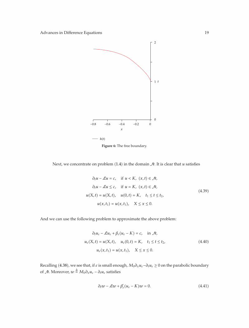
h(t)
Figure 6: The free boundary.
Next, we concentrate on problem (1.4) in the domainN. It is clear that u satisfies
∂tu − Lu = c, if u < K, (x, t) ∈ N,
∂tu − Lu ≤ c, if u = K, (x, t) ∈ N,
u(X, t) = u(X, t), u(0, t) = K, t1 ≤ t ≤ t2,
u(x, t1) = u(x, t1), X ≤ x ≤ 0.
(4.39)
And we can use the following problem to approximate the above problem:
∂tuε − Luε + βε(uε −K) = c, in N,
uε(X, t) = u(X, t), uε(0, t) = K, t1 ≤ t ≤ t2,
uε(x, t1) = u(x, t1), X ≤ x ≤ 0.
(4.40)
Recalling (4.38), we see that, if ε is small enough,M0∂xuε−∂tuε ≥ 0 on the parabolic boundary
of N. Moreover,w Δ= M0∂xuε − ∂tuε satisfies
∂tw − Lw + β′ε(uε −K)w = 0. (4.41)
20 Advances in Difference Equations
Applying the comparison principle, we obtain
M0∂xuε − ∂tuε = w ≥ 0 in N. (4.42)
As the method in the proof of Theorem 3.3, we can show that uε weakly converges to u inW2,1
p (N) and (4.30) is obvious.On the other hand, we see thatM∂xu + ∂tu ≥ 0 inN for any positive number M from
(3.26) and (3.27). So,
M0∂xu ± ∂tu ≥ 0 in N, (4.43)
which means that there exists a uniform cone such that the free boundary should lies inthe cone. As the method in [9], it is easy to derive that h(t) ∈ C0,1[t1, t2]. Moreover h(t) ∈C∞[t0, t2] can be deduced by the bootstrapmethod. Since t2 is arbitrary and the free boundaryis a vertical line while t ∈ (0, t0), then h(t) ∈ C0,1[0, T0) ∩ C∞[t0, T0).
5. Numerical Results
Applying the binomial tree method to problem (1.4), we achieve the following numericalresults—Figure 6:
Plot of the optimal exercise boundary h(t) is a function of t. The parameter values usedin the calculations are r = 0.2, q = 0.1, σ = 0.3, L = 1, K = 1.5, c = 0.5, T = 2, and n = 3000.In this case, the free boundary is increasing with x(0) = 0. The numerical result is coincidedwith that of our proof (see Figure 6).
Acknowledgments
The project is supported by NNSF of China (nos. 10971073, 11071085, and 10901060) andNNSF of Guang Dong province (no. 9451063101002091).
References
[1] M. Sırbu, I. Pikovsky, and S. E. Shreve, “Perpetual convertible bonds,” SIAM Journal on Control andOptimization, vol. 43, no. 1, pp. 58–85, 2004.
[2] M. Sırbu and S. E. Shreve, “A two-person game for pricing convertible bonds,” SIAM Journal onControl and Optimization, vol. 45, no. 4, pp. 1508–1539, 2006.
[3] P. Wilmott, Derivatives, the Theory and Practice of Financial Engineering, John Wiley & Sons, New York,NY, USA, 1998.
[4] Y. Kifer, “Game options,” Finance and Stochastics, vol. 4, no. 4, pp. 443–463, 2000.[5] Y. Kifer, “Error estimates for binomial approximations of game options,” The Annals of Applied
Probability, vol. 16, no. 2, pp. 984–1033, 2006.[6] C. Kuhn and A. E. Kyprianou, “Callable puts as composite exotic options,”Mathematical Finance, vol.
17, no. 4, pp. 487–502, 2007.[7] A. E. Kyprianou, “Some calculations for Israeli options,” Finance and Stochastics, vol. 8, no. 1, pp.
73–86, 2004.[8] F. Black and M. Scholes, “The pricing of options and coperate liabilities,” Journal of Political Economy,
vol. 81, pp. 637–659, 1973.
Advances in Difference Equations 21
[9] Z. Yang and F. Yi, “A free boundary problem arising from pricing convertible bond,” ApplicableAnalysis, vol. 89, no. 3, pp. 307–323, 2010.
[10] A. Friedman, “Parabolic variational inequalities in one space dimension and smoothness of the freeboundary,” Journal of Functional Analysis, vol. 18, pp. 151–176, 1975.
[11] A. Blanchet, “On the regularity of the free boundary in the parabolic obstacle problem. Applicationto American options,”Nonlinear Analysis: Theory, Methods & Applications, vol. 65, no. 7, pp. 1362–1378,2006.
[12] A. Blanchet, J. Dolbeault, and R.Monneau, “On the continuity of the time derivative of the solution tothe parabolic obstacle problemwith variable coefficients,” Journal deMathematiques Pures et Appliquees.Neuvieme Serie, vol. 85, no. 3, pp. 371–414, 2006.
[13] L. Caffarelli, A. Petrosyan, and H. Shahgholian, “Regularity of a free boundary in parabolic potentialtheory,” Journal of the American Mathematical Society, vol. 17, no. 4, pp. 827–869, 2004.
[14] A. Petrosyan and H. Shahgholian, “Parabolic obstacle problems applied to finance,” in RecentDevelopments in Nonlinear Partial Differential Equations, vol. 439 of Contemporary Mathematics, pp. 117–133, American Mathematical Society, Providence, RI, USA, 2007.
[15] A. Friedman, “Stochastic games and variational inequalities,” Archive for Rational Mechanics andAnalysis, vol. 51, pp. 321–346, 1973.
[16] A. Friedman, Variational Principles and Free-Boundary Problems, Pure and Applied Mathematics, JohnWiley & Sons, New York, NY, USA, 1982.
[17] D. Gilbarg and N. S. Trudinger, Elliptic Partial Differential Equations of Second Order, vol. 224 ofGrundlehren der Mathematischen Wissenschaften, Springer, Berlin, Germany, 2nd edition, 1983.
[18] O. A. Ladyzenskaja, V. A. Solonnikov, and N. N. Uralceva, Linear and Quasi-linear Equations of ParabolicType, American Mathematical Society, Providence, RI, USA, 1968.
[19] F. Yi, Z. Yang, and X. Wang, “A variational inequality arising from European installment call optionspricing,” SIAM Journal on Mathematical Analysis, vol. 40, no. 1, pp. 306–326, 2008.
[20] K. Tso, “On Aleksandrov, Bakel’man type maximum principle for second order parabolic equations,”Communications in Partial Differential Equations, vol. 10, no. 5, pp. 543–553, 1985.