A TWO LAYER MODEL FOR WAVE DISSIPATION IN SEA ICE

Graig SutherlandNumerical Environmental Prediction Research

Environment and Climate Change Canadagraigory.sutherland@canada.ca

Jean RabaultDepartment of Mathematics

University of Oslojeanra@math.uio.no

Kai H. ChristensenNorwegian Meteorological Institute

kaihc@met.no

Atle JensenDepartment of Mathematics

University of Osloatlej@math.uio.no

October 10, 2018

ABSTRACT

Sea ice is highly complex due to the inhomogeneity of the physical properties (e.g. temperatureand salinity) as well as the permeability and mixture of water and a matrix of sea ice and/or seaice crystals. Such complexity has proven itself to be difficult to parameterize in operational wavemodels. Instead, we assume that there exists a self-similarity scaling law which captures the firstorder properties. Using dimensional analysis, an equation for the kinematic viscosity is derived whichis proportional to the wave frequency and the ice thickness squared. In addition, the model allows fora two-layer structure where the oscillating pressure gradient due to wave propagation only exists in afraction of the total ice thickness. These two assumptions lead to a spatial dissipation rate that is afunction of ice thickness and wavenumber. The derived dissipation rate compares favourably withavailable field and laboratory observations.

Keywords Waves · Sea ice ·Wave dissipation ·Wave-ice interaction

1 Introduction

The marginal ice zone (MIZ) can be defined as the interfacial region of the cryosphere between the open ocean andconsolidated pack ice, and is the region of the cryosphere that is most affected by surface ocean waves. The MIZ isa complex and highly variable sea ice environment, which comprises many individual floes of arbitrary shape and avariety of ice types from new ice to fragmented multi-year ice. While surface waves are expected to be a dominantprocess controlling the sea ice size distribution and extent of the MIZ, there still exist large uncertainties about the exactmechanisms for wave attenuation in sea ice (Williams et al., 2013, 2017; Kohout et al., 2014; Meylan et al., 2014). Inaddition to affecting the floe size distribution, the attenuation of surface gravity waves is also important in controllingthe extent of the MIZ via the wave radiation stress (Liu et al., 1993; Williams et al., 2017).

The two predominant sources for the attenuation of wave energy propagating into an ice field are due to scattering,which is a conservative process that redistributes energy in all directions, and dissipative processes due to friction(viscosity), inelastic collisions and the breakup of ice floes (Squire et al., 1995; Squire, 2007; Doble & Bidlot, 2013;Williams et al., 2013). The relative importance of scattering and dissipative processes is still unclear and a topic ofactive research (Squire & Montiel, 2016). Theoretical studies of wave scattering suggest that dissipative mechanismsmay be dominant for small floe sizes (Kohout & Meylan, 2008; Bennetts & Squire, 2012), relative to the incomingwavelength, as would be found in frazil and pancake ice fields in the MIZ (Doble et al., 2015). In addition, Ardhuinet al. (2016) found that dissipative mechanisms dominated the wave attenuation for narrow banded swell travellingseveral hundred kilometres into the pack ice (Wadhams & Doble, 2009), which suggests that wave scattering by ice

arX

iv:1

805.

0113

4v3

[ph

ysic

s.ao

-ph]

9 O

ct 2

018

WAVES IN SEA ICE- OCTOBER 10, 2018

floes is more complex. Recent studies on wave attenuation in the MIZ have focused on dissipative processes (Dobleet al., 2015; Rogers et al., 2016; Cheng et al., 2017) as these are expected to be dominant in the MIZ.

There are many factors which contribute to the difficulty of determining wave attenuation in sea ice. First, fieldobservations are difficult to obtain and thus remain relatively sparse. To obtain the wave attenuation requires collocatedobservations of the wave amplitude and wave direction at several frequencies over spatial distances on the order ofkilometres. In addition, it is not only the sea ice which affects the spectral energy of the surfaces waves as the windforcing and the nonlinear transfer of energy can also represent significant contributions in the lower ice concentrationsfound in the MIZ (Li et al., 2015, 2017). Second, while laboratory experiments of waves and sea ice circumvent manyof the problems encountered in interpreting field data, there exist many problems associated with scaling laboratoryexperiments to larger scales. For instance, it is desirable to not have the bottom influence surface experiments, whichrequires kD > 1 where k is the wavenumber and D is the water depth. Furthermore, it is also desirable to performexperiments with relatively linear waves and thus limiting the wave steepness to ak < 0.1 where a is the wave amplitude.For a wave tank of depth D = 1 m, these two criteria require amplitudes to be less than 0.1 m and frequencies to begreater than 0.5 Hz. This is why most laboratory experiments are performed with low amplitude and high frequencywaves. See Rabault et al. (2018) for a discussion on difficulties in scaling laboratory experiments.

There exist many models that describe viscous dissipation in a frazil and pancake ice field, with various degreesof consistency with observations. Weber (1987) assumed that the ice layer could be modelled as a highly viscouscontinuum where the dynamics in the ice layer consist of a balance between pressure and viscous forces, i.e. “creepingmotion” or Stokes flow (not to be confused with ice creep (e.g. Wadhams, 1973)), and the wave dissipation exists solelyin the ocean boundary layer below the sea ice. In this case, Weber (1987) showed that the sea ice layer effectively haltsthe horizontal motion of the water at the ice-water interface and the spatial dissipation is identical to the inextensible(i.e. non-elastic) limit for waves under a surface cover (Lamb, 1932; Phillips, 1977; Sutherland et al., 2017a). Thisparameterization compared well with available field observations in the MIZ at the time (Wadhams et al., 1988) with aneddy viscosity under the ice between 2 and 4 orders of magnitude greater than the molecular value for sea water. Whilethis model has been shown to also compare well with later observations (Sutherland & Gascard, 2016; Rabault et al.,2017), it does require the fitting of an eddy viscosity, which is required to vary by several orders of magnitude to beconsistent with observations and such large values may not be physically realistic (Stopa, 2016).

Other studies on wave dissipation have focused on the dissipation of wave energy within the sea ice, and modelled thesea ice as a viscous (Keller, 1998; De Carolis & Desiderio, 2002) or viscoelastic (Wang & Shen, 2010b) layer overan inviscid (Keller, 1998; Wang & Shen, 2010b) or viscid ocean (De Carolis & Desiderio, 2002). While there existconsistencies between these models and available observations (e.g. Newyear & Martin, 1999), all of these modelsrequire the rheological properties of the sea ice to be empirically determined from observations of wave dissipation.In addition, these models require solving a complex dispersion relation to determine the most physically significantsolution, which is not always straightforward and simple (see Mosig et al., 2015). The complexity of these modelsincrease the computational expense of implementation into numerical prediction systems, in addition to having atendency of obscuring the physical interpretation.

There has been significant work on using available observations for testing (Rogers et al., 2016) and calibrating (Chenget al., 2017) the viscoelastic model of Wang & Shen (2010b) to be implemented in WAVEWATCH III R© (TheWAVEWATCH III R© Development Group (WW3DG), 2016). The viscoelastic model is particularly appealing, in theory,due to the use of one rheological model to predict wave propagation in all types of sea ice. This ultimately requirescareful tuning of the viscous and elastic parameters over a large variety of sea ice types and conditions. However,field (Rogers et al., 2016; Cheng et al., 2017) and laboratory (Wang & Shen, 2010a; Zhao & Shen, 2015) studies havestruggled to predict wave attenuation across a broad range of frequencies and ice types. For frazil and pancake ice, thesestudies also require a non-zero elastic term in order to be consistent with observations, but as of yet there does not exista strong physical explanation for the inclusion of such an elastic term, which must be tuned from available observationsof wave attenuation. Due to the requirement of empirically fitting the sea ice rheology, the viscoelastic model alsoprovides an extra term for fitting, and thus should provide improved consistency with observations independent ofwhether the physics are correct.

The theories described here all assume the sea ice has a vertically homogeneous structure, which is rare in reality asthere exists large vertical gradients in temperature, and often the bulk salinity, within the sea ice (Cox & Weeks, 1974).The temperature and bulk salinity, along with the related fraction of solid ice parameter, affect many properties of thesea ice (Hunke et al., 2011), for example porosity and permeability, that it seems natural that this vertical structure willalso affect wave propagation. In this paper, a new parameteriztion for wave dissipation is presented, which allows for atwo-layer structure within the ice. This model assumes wave motion, i.e. an oscillating pressure gradient, in a fractionof the sea ice and that the remainder of the sea ice is too viscous to render it effectively solid over the temporal scales oftypical ocean waves. The viscosity is derived using dimensional analysis, which assumes the existence of a universal

2

WAVES IN SEA ICE- OCTOBER 10, 2018

highly viscous layer

water layer

impermeable layer

(1 )hi

0

hi

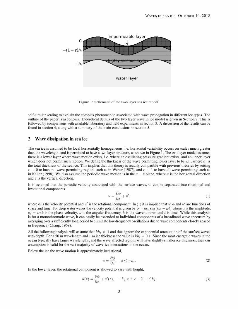
Figure 1: Schematic of the two-layer sea ice model.

self-similar scaling to explain the complex phenomenon associated with wave propagation in different ice types. Theoutline of the paper is as follows. Theoretical details of the two layer wave in ice model is given in Section 2. This isfollowed by comparisons with available laboratory and field experiments in section 3. A discussion of the results can befound in section 4, along with a summary of the main conclusions in section 5.

2 Wave dissipation in sea ice

The sea ice is assumed to be local horizontally homogeneous, i.e. horizontal variability occurs on scales much greaterthan the wavelength, and is permitted to have a two layer structure, as shown in Figure 1. The two layer model assumesthere is a lower layer where wave motion exists, i.e. where an oscillating pressure gradient exists, and an upper layerwhich does not permit such motion. We define the thickness of the wave permitting lower layer to be εhi, where hi isthe total thickness of the sea ice. This implies that this theory is readily compatible with previous theories by settingε → 0 to have no wave-permitting region, such as in Weber (1987), and ε → 1 to have all wave-permitting such asin Keller (1998). We also assume the periodic wave motion is in the x− z plane, where x is the horizontal directionand z is the vertical direction.

It is assumed that the periodic velocity associated with the surface waves, u, can be separated into rotational andirrotational components

u =∂φ

∂x+ u′, (1)

where φ is the velocity potential and u′ is the rotational component. In (1) it is implied that u, φ and u′ are functions ofspace and time. For deep water waves the velocity potential is given by φ = acp sin (kx− ωt) where a is the amplitude,cp = ω/k is the phase velocity, ω is the angular frequency, k is the wavenumber, and t is time. While this analysisis for a monochromatic wave, it can easily be extended to individual components of a broadband wave spectrum byaveraging over a sufficiently long period to eliminate low-frequency oscillations due to wave components closely spacedin frequency (Chang, 1969).

All the following analysis will assume that khi � 1 and thus ignore the exponential attenuation of the surface waveswith depth. For a 50 m wavelength and 1 m ice thickness the value is khi = 0.1. Since the most energetic waves in theocean typically have larger wavelengths, and the wave affected regions will have slightly smaller ice thickness, then ourassumption is valid for the vast majority of wave-ice interactions in the ocean.

Below the ice the wave motion is approximately irrotational,

u =∂φ

∂x, z ≤ −hi. (2)

In the lower layer, the rotational component is allowed to vary with height,

u(z) =∂φ

∂x+ u′(z), −hi < z < −(1− ε)hi. (3)

3

WAVES IN SEA ICE- OCTOBER 10, 2018

Since khi � 1 we can safely omit the exponential decay with depth of the irrotational component of the wave velocity.In the upper layer, the ice is essentially a deformable solid body and there are no velocity gradients within this region.

Rotational shear only exists in the wave permitting region over the depth range −hi < z < −(1− ε)hi. Therefore, thedissipation of wave energy can be calculated from the irrotational shear (Phillips, 1977) over this region,

∂E

∂t= −ρν

∫ −(1−ε)hi

−hi

(∂u′

∂z

)2

dz, (4)

where E is the wave energy, ρ is the viscous layer density and ν is the effective kinematic viscosity associated with thedissipation of wave energy. To keep the solution general, we assume that velocity in the wave permitting region willhave the same structure as the irrotational solution, but with a decrease in amplitude and a phase lag, i.e.

u = Γaω cos (kx− ωt− ψ), −hi < z < −(1− ε)hi, (5)

where 0 ≤ Γ ≤ 1 is the amplitude reduction and ψ is the phase lag, and are allowed to be functions of z. From (5) wecan estimate the rotational component of the velocity

u′ = u− ∂φ

∂x= Γaω cos (kx− ωt− ψ)− aω cos kx− ωt). (6)

Assuming that the phase lag ψ is small, such that second order effects can be neglected, (6) becomes

u′ = aω [(Γ− 1) cos (kx− ωt) + Γψ sin (kx− ωt)]

= aω[√

(Γ− 1)2 + (Γψ)2 sin (kx− ωt− θ)],

(7)

where θ = tan−1(Γ− 1)/(Γψ).

Now, in order to simplify the problem, we will estimate the mean shear over the wave permitting region of thicknessεhi using boundary conditions (7) and (2), therefore

∂u′

∂z=aw [(Γ− 1) cos (kx− ωt) + Γψ sin (kx− ωt)]

εhi. (8)

By taking Γ = Γ0 and ψ = ψ0 evaluated at z = −(1− ε)hi, we can estimate the integral of (4) to be∫ 0

−hi

(∂u′

∂z

)2

dz =1

2

(aω

εhi

)2 [1− 2Γ0 + (1 + ψ2

0)Γ20

]εhi. (9)

Substituting (9) into (4), defining ∆0 = 1− 2Γ0 + (1 + ψ20)Γ2

0, and using the definition for wave energy E = ρga2/2,where g is the acceleration due to gravity, allows for (4) to be written as

∂E

∂t= −νω

2∆0

gεhiE. (10)

Using the definition for the temporal dissipation rate,

β = − 1

2E

∂E

∂t, (11)

along with (10) and assuming the dispersion relation to be that of open water, ω2 = gk, allows for (11) to be written as

β =νk∆0

2εhi. (12)

Equation (12) is equivalent to the classical equation for wave dissipation under an inextensible surface cover (Lamb,1932) assuming a no-slip boundary condition at z = −(1− ε)hi (i.e. ∆0 → 1), and with a boundary layer thickness ofεhi.

Assuming the wave dissipation is small, such that β � ω, the temporal dissipation rate can be related to the spatialdissipation rate, which we will denote α, using the group velocity, i.e. cg = β/α (Gaster, 1962). Using the groupvelocity in open water, cg = ω/(2k), allows (12) to be converted to a spatial dissipation rate

α =ν∆0k

2

ωεhi. (13)

4

WAVES IN SEA ICE- OCTOBER 10, 2018

The most uncertain aspect of (13) is the viscosity of the grease ice ν, which is undoubtedly a complicated function ofthe ice micro-structure. However, some insight might be gained by looking at the relevant macroscopic ice propertieswith regards to wave dissipation in order to look for a self-similar, i.e. non-dimensional, solution. At the macroscopiclevel the grease ice can be summarized by two factors: the viscosity ν and the thickness hi. To first order, and thusignoring wave amplitude effects on the grease ice and using the assumption that khi � 1, the relevant parameters forwave dissipation are then ν, hi and ω. According to the Π theorem (Buckingham, 1914) the problem can be defined byexactly one non-dimensional value and the grease ice viscosity must scale as

ν = Aωh2i , (14)

where A is a constant.

We will use a constant A = 0.5ε2 in order for (14) to be equivalent to the classic Stokes boundary layer (Lamb, 1932;Phillips, 1977) for a boundary layer depth of εhi. The ice viscosity is then

ν =1

2ω (εhi)

2. (15)

Substituting (15) into (13) gives

α =1

2∆0εhik

2. (16)

Equation (16) gives an estimate of the spatial decay rate of surface waves as a function of the wavenumber and icethickness, with two unknowns that range in value between zero and one. However, if we are to assume self-similarityfor wave dissipation in grease ice layers, then α ∝ hik

2 should be valid and the constant of proportionality can bedetermined from experiments. That being said we believe there is some physical interpretation to the constant ofproportionality, which is explored next.

2.1 Determining ∆0

The ∆0 term determines the boundary condition imposed on the bottom of the ice. A no-slip boundary condition, i.e.Γ0 → 0, leads to ∆0 = 1. This was shown by Weber (1987) to be valid to first order for a highly viscous ice layer,and provided consistent results with observations in the MIZ made by Wadhams et al. (1988). However, Ardhuin et al.(2018) suggest weakening the no-slip condition depending on the ratio of the floe size to the wavelength and devisean empirical formulation which dramatically reduces the attenuation rate for wavelengths greater than 3 times thedominant floe size. In this formulation there is no explicit mentioning whether this reduction is due to the amplitude,phase lag, or both of the ice motion relative to the water.

In the absence of data on the issue we will assume a no-slip condition and take ∆0 = 1. This provides an upper boundfor the wave dissipation in the sea ice and can easily be modified if evidence is presented for the relative ice-watermotion.

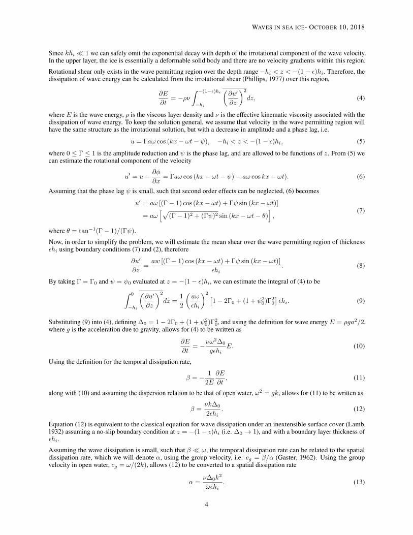
Figure 2 shows ∆0 as a function of Γ0 for various small phase lags ψ0. It can easily be seen that if the motion is muchsmaller at the surface than in the water that ∆0 ≈ 1 is a valid approximation. To first order, the phase lag is onlyimportant when there is negligible dissipation in the sea ice layer, which would occur in either very thin ice layers ormore impermeable ice layers where εhi is very small.

2.2 Determining ε

As the determination of ε is most likely linked with the sea ice micro-structure this term is difficult to estimate. Itseems reasonable that it would be related to the permeability of the sea ice, which is a function of ice temperature,salinity and ice volume fraction, and that using the law of fives (Golden et al., 2007), which states that ice transitionsfrom impermeable to permeable when the ice temperature reaches −5◦C and bulk salinity is 5 parts per thousand,may provide a good starting point. For operational purposes it may be useful to estimate ε as a function of sea iceconcentration, with lower sea ice concentrations having larger values of ε, with the argument that more water will leadto more (relatively) warm sea ice which is more permeable. Such a parameterization would also be consistent withobservations of wave attenuation being several orders of magnitude greater in the MIZ (Doble et al., 2015) than in packice (Wadhams et al., 1988; Meylan et al., 2014). It can also be used as an empirical parameter to be fit a posteriori, notunlike current viscous ice models, from available data.

For ε→ 1, the rotational wave motion exists throughout the ice layer and the effective viscosity is given by ν = ωh2i /2.This scenario of ε→ 1 provides an upper limit on the wave dissipation in the sea ice of α = hik

2/2. In the limit asε→ 0, there is no wave dissipation within the sea ice and the ice layer is identical to that assumed by Weber (1987).

5

WAVES IN SEA ICE- OCTOBER 10, 2018

10 2 10 1 100

0

10 2

10 1

100

0

0 = 00 = 100 = 20

Figure 2: Value of ∆0 as a function of velocity amplitude reduction Γ0 for various phase lags ψ0.

3 Comparisons with previous experiments

Simultaneous observations of wave propagation and ice thickness are rare in the field and are predominantly restrictedto laboratory experiments. In this section, (16) is compared with available observations and it assumed that ∆0 = 1, i.e.the ice motion is negligible compared to the water motion. However, since we do not have knowledge of the relativeice-water motion then uncertainty in ∆0 will be included in the least-squares fit of ε.

Three laboratory experiments (Newyear & Martin, 1997; Wang & Shen, 2010a; Zhao & Shen, 2015) and one fieldcampaign (Doble et al., 2015) are used, as these experiments provide both estimates of wave attenuation and icethickness. The laboratory studies are performed with mechanically generated monochromatic linear waves, which allowfor a direct comparison of our model with the observed wave dissipation. A summary of the least-squares fits withthe laboratory data can be found in Table 1. Interpreting field data is decidedly more difficult as the wave field oftenconsists of a broadband spectrum and the wind input and nonlinear terms can also have a non-negligible contribution tothe spectral energy (Li et al., 2015, 2017). It is important to keep this in mind, that the wave dissipation due to the seaice might not be the only process affecting the wave spectral energy, when comparing field observations with theoreticalmodels for wave dissipation.

Experiment hi / cm ε R2

Newyear & Martin (1997) 11.3 0.70 ± 0.01 0.9814.6 0.60 ± 0.02 0.92

Wang & Shen (2010a) 9.0 0.56 ± 0.03 0.858.9 0.64 ± 0.03 0.90

Zhao & Shen (2015) 2.5 0.34 ± 0.03 0.774.0 0.94 ± 0.03 0.987.0 0.85 ± 0.09 0.72

Table 1: Summary of fitting results using (16) with data from available laboratory experiments. In all cases it is assumedthat ∆0 = 1.

It is often difficult to properly scale all the relevant wave-ice interaction processes in laboratory experiments (seeRabault et al., 2018) given the geometric constraints of laboratory basins. It is not always possible to scale the icethickness and wavenumber such that khi � 1. Also, while field observations of the dispersion relation waves inice show little deviation from open water values (Marchenko et al., 2017), this is not always the case in laboratory

6

WAVES IN SEA ICE- OCTOBER 10, 2018

0.0

2.5

5.0

7.5

10.0

k/m

1

aNewyear and Martin (1997)Wang and Shen (2010)Zhao and Shen (2015)

0 5 10 15 20 25 30 35 40h 1

i /m 1

0.0

2.5

5.0

7.5

10.0

k 0/m

1

bkh = 1kh = 0.5kh = 0.1

Figure 3: a Observed values of the wavenumber k as a function of inverse ice thickness h−1i and b wavenumbercalculated from the frequency using the open water relation k0 = ω2/g as a function of inverse ice thickness. The blacklines show various values for constant khi. The experiments correspond to those in Table 1.

experiments (Newyear & Martin, 1997). Figure 3 shows k vs h−1i for the observed wavenumber (3a) and the theoreticalopen water wavenumber k0 = ω2/g (Figure 3b).

Figure 3 shows relatively large values of khi in the Newyear & Martin (1997) experiment with khi → 1 for highfrequencies with the effect being greater for the larger (smaller) ice thickness (inverse ice thickness). There is alsoa noticeable deviation from the open water value for these higher frequencies. In the experiment by Wang & Shen(2010a), khi values are all smaller than in Newyear & Martin (1997) with values ranging 0.1 < khi < 0.5 and littledeviation from the open water dispersion relation. The khi values in Zhao & Shen (2015) are smaller yet with theseapproximately equal to khi = 0.1.

3.1 Laboratory experiment of Newyear & Martin (1997)

This study was one of the first to measure wave dissipation due to frazil ice in a controlled laboratory experiment. Twoexperiments were performed with different frazil ice thicknesses: one experiment was with an ice thickness of 11.3cm and the other was 14.6 cm thick. Figure 4 shows results for the wave dissipation from the two experiments, takenfrom Tables 1 and 2 in Newyear & Martin (1997). Comparisons with (16) are made assuming ε ≈ 1 (dash-dot line) andε = 0.7 (solid line).

While the agreement between the observations and (16) is qualitatively quite good, there is some deviation at the higherfrequencies for the 14.6 cm experiment. At these high frequencies, khi ≈ 1 (Figure 3) and the assumptions leading to(15) of a relatively thin layer with respect to the wavelength are no longer be valid. These frequencies also correspondto where the dispersion relation deviated significantly from the open water relation for experiment 2 (hi = 14.6 cm) withthe observed wavenumber being 70-80% of the expected open water value (Newyear & Martin, 1999). For experiment1 (hi = 11.3 cm) the maximum deviation of the dispersion relation relative to the open water is much less with theobserved wavenumber being 90% of the open water value at the highest frequencies.

3.2 Laboratory experiment of Wang & Shen (2010a)

This study was one of many performed as part of the REduced ice Cover in the ARctic Ocean (RECARO) project inthe Arctic Environmental Test Basin at Hamburg Ship Model Basin (HSVA), Germany (Wilkinson et al., 2009). Twoexperiments were performed with each having a very similar mean ice thickness of 8.9 cm and 9.0 cm respectively.

7

WAVES IN SEA ICE- OCTOBER 10, 2018

0.6 0.8 1.0 1.2 1.4 1.6f/Hz

0.0

0.5

1.0

1.5

2.0

2.5

3.0

3.5

4.0

/m1

hi = 11.3 cmhi = 14.6 cm

= 0.70= 1.00= 0.60= 1.00

Figure 4: Comparison with results from Newyear & Martin (1997). Dots show observations for a given ice thickness hiand the curves show the results from (16) for different values of ε.

The sea ice in this experiment is formed in a similar manner as Newyear & Martin (1997). A comparison of (16) andthe dissipation rates observed by Wang & Shen (2010a), from their Tables 1 and 2, can be found in Figure 5. Again,the comparison is quite good, but now the deviations from theory occur for the lower frequencies with the smallestdissipation rates. It is unclear why the dissipation is under-predicted at low frequencies, however the same deviationwas also observed by Wang & Shen (2010a) in fitting the viscoelastic model (Wang & Shen, 2010b). The observedwavenumber in this experiment was similar to the open water value with a maximum deviation of 10%.

3.3 Laboratory experiment of Zhao & Shen (2015)

These results were obtained from a subsequent experiment at the HSVA during 2013. In this experiment there werethree distinct ice types: thin frazil ice (2.5 cm thickness), a frazil and pancake ice mixture (4.0 cm thickness) and abroken floe field (7.0 cm thickness). The results from each, as recorded in their Table 3, are shown in Figure 6.

Again, the comparisons are good with both the 4.0 cm and 7.0 cm thicknesses being well explained by (16) for largevalues of ε. For the thin frazil ice of 2.5 cm thickness, the observed wave dissipation had a very small ε of 0.34, whichis most likely due to the relative motion of the ice, i.e. ∆0 < 1, which stands to reason would be greater for very thinice layers than thicker layers.

For the thicker ice, the same under-prediction of the wave dissipation relative to the observed value was observed,consistent with the results of Wang & Shen (2010a). Zhao & Shen (2015) also found that the viscoelastic modelof Wang & Shen (2010b) under estimated α at low frequencies.

3.4 Field observations of Doble et al. (2015)

Simultaneous field measurements of ice thickness and wave attenuation are rare, but a recent publication by Dobleet al. (2015) utilized detailed observations of the ice type and thickness (Doble et al., 2003) to investigate the waveattenuation characteristics for a frazil and pancake ice field in the Weddell Sea. Doble et al. (2015) found that the spatialenergy attenuation rate was linearly related to the ice thickness according to

αD15∗ = 0.2T−2.13heq, (17)

where T is the wave period and heq is an equivalent ice thickness, i.e. heq = Φhi where Φ is the ice volume fraction.Note that the energy attenuation rate is related to the attenuation rate in amplitude by α∗ = 2α and (16) is multiplied by2 for comparisons with Doble et al. (2015). The ice volume fraction used by Doble et al. (2015) was 0.7 for pancake iceand 0.4 for frazil ice with estimates of the relative abundance of each in order to obtain a mean heq. The ice thickness

8

WAVES IN SEA ICE- OCTOBER 10, 2018

0.4 0.5 0.6 0.7 0.8 0.9 1.0 1.1 1.2f/Hz

0.0

0.2

0.4

0.6

0.8

1.0

/m1

hi = 9.0 cmhi = 8.9 cm

= 0.56= 1.00= 0.64= 1.00

Figure 5: Comparison with results from Wang & Shen (2010a). Dots show observations for a given ice thickness hiand lines show (16) for different values of ε.

was measured during the initial deployment of the waves and modelled forward in time using a 1-D thermodynamicmodel coupled to a 2-D redistribution scheme (Doble et al., 2003). While (16) predicts α ∝ hi, it also predicts thedependence on the wave period to be α ∝ T−4 in contrast with (17), which has a period dependence of α ∝ T−2.13.

Figure 7 shows a comparison of the observations of the wave energy attenuation rate by Doble et al. (2015) with α∗calculated by multiplying (16) by 2. Figure 7 shows both a power law fit - black dashed line - as well as a least squaresfit to (16) - shown in blue - with corresponding R2 values of 0.98 and 0.96 respectively. The least-squares fit is for ε/Φ,which gives a best estimate of ε/Φ = 1.26 ± 0.05. For pure grease ice φ = 0.4 implies that ε = 0.50 and for an allpancake field Φ = 0.7 giving ε = 0.88.

First, in order to compare (17) with (16), it is important to relate heq with the ice layer thickness hi. This is important as(16) depends on the thickness of the viscous layer, comprising a mixture of water and ice, and the thickness associatedwith only the ice component is not directly applicable. While the relative abundance of frazil and pancake ice is notknown, the problem can be constrained by assuming a 100% frazil ice field and a 100% pancake ice field Doble et al.(2015). Using heq = Φhi and (16) multiplied by 2 to get α∗ gives α∗/heq = εk2/(Φ), which allows for a comparisonof the observations of Doble et al. (2015) and our model. Figure 7 shows the comparison of (16), with different valuesof Φ and ε consistent with laboratory experiments, and the observations of Doble et al. (2015).

For wave periods below 10 s, the frequency response of α∗/heq is approximately constant, which is similar to the“roll-over” observed in the attenuation rate from previous experiments at low wave periods (Wadhams et al., 1988) and shownrecently to be due the input from the wind and nonlinear effects (Li et al., 2017). Thus, wave dissipation is not expectedto be the predominant process affecting wave energy at these frequencies and (16) would not be applicable. For waveperiods greater than 14 s, the frequency response of α∗/heq also becomes relatively flat, which is a bit puzzling and it isnot clear as to what could cause such a frequency response. It is possible that it could be related to the smaller signalto noise ratio for wave elevations at high frequencies as the noise level increases as ω2 (Sutherland et al., 2017b). Inaddition, the nonlinear transfer of wave energy between frequencies could also be relatively important (Li et al., 2017)as wave dissipation is much lower at these high wave periods.

For the periods between 10 s and 14 s (black dots in Figure 7), α∗/heq decreases rapidly with increasing wave periodand (16) performs qualitatively well. A power law is fitted in this range of wave periods with an r-squared value of0.98 and giving a period dependence of α ∝ T−3.76, with a standard error in the exponent of −3.76± 0.33, consistentwith (16) which predicts α ∝ T−4. While it’s not difficult to argue that the wind input and nonlinear transfer are lessthan the dissipation due to sea ice at these frequencies, i.e. periods greater than the wind-input terms and periods lessthan where nonlinear transfer becomes larger, it is still conjecture at this point without calculating these terms. Thegood agreement between the magnitude of the observations and (16) for Φ = 0.4 is most likely fortuitous as the other

9

WAVES IN SEA ICE- OCTOBER 10, 2018

0.4 0.5 0.6 0.7 0.8 0.9 1.0 1.1 1.2f/Hz

0.0

0.2

0.4

0.6

0.8

1.0

/m1

hi = 2.5 cmhi = 4.0 cmhi = 7.0 cm

= 0.34= 1.00= 0.94= 1.00= 0.85= 1.00

Figure 6: Comparison with results from Zhao & Shen (2015). Dots show observations for different ice thicknesses hiand lines show (16) for different values of ε.

spectral source terms will contribute some fraction of the observed attenuation rate. Plus, it is unlikely that the ice fieldwas all frazil ice during the observation period. This will be discussed further later on.

4 Discussion

One uncertainty in using (16) as a model for wave dissipation is the determination of ε. However, since α in (16) islinearly related to ε, their relative uncertainties are also linear, i.e. a 50% uncertainty in ε will correspond to a 50%uncertainty in α. Just to clarify, (16) is a model for the wave dissipation in the ice layer and neglects viscous dissipationoccurring below the ice - identical to the dissipative models of Keller (1998) and Wang & Shen (2010b). As ε→ 0, theviscous dissipation below the ice will no longer be negligible compared to the dissipation occurring within the ice. Thisshortcoming can be addressed by adding the wave dissipation associated with the boundary layer under the ice (see Liu& Mollo-Christensen, 1988), and this has been used in studies of wave dissipation for waves with long periods andsmall amplitudes over long distances into the pack ice (Ardhuin et al., 2016) where one would expect ε to be small asthere will be limited wave motion in solid ice. For example, Ardhuin et al. (2016) use the wave dissipation due to theboundary layer under the sea ice (Liu & Mollo-Christensen, 1988), which we will denote αLM88 and is given by

αLM88 =1

2dk2 (18)

where d is the boundary layer under the ice calculated using d =√

2νw/ω and νw is the molecular kinematic viscosityof sea water. Ardhuin et al. (2016) multiply (18) by a factor of 12 in order to reproduce the observed wave heights.Since d ∝ ν0.5w a factor of 12 increase in α corresponds with a factor of 144 increase in νw. However, it can easily beshown that α calculated using (16) is related to αLM88 by

α =εhidαLM88. (19)

Note that the frequency dependence of d leads to αLM88 ∝ T−3.5, which is slightly different than (16) where α ∝ T−4.Ardhuin et al. (2016) used a molecular kinematic viscosity of sea water of νw = 1.83× 10−6 m2s−1, which gives d onthe order of 10−3 m for typical wave frequencies. Using an ice thickness on the order of 1 m gives an ε on the order of10−2 to reproduce the empirical factor of 12 used by Ardhuin et al. (2016). This shows that wave motion only needs toexist a few centimetres in the ice layer in order to produce much higher dissipation rates than would be expected in theboundary layer under the ice. This variability in ε may also explain the much greater wave dissipation observed in fraziland pancake ice (Newyear & Martin, 1997; Doble et al., 2015; Rabault et al., 2017) compared to measurements in packice (Meylan et al., 2014; Ardhuin et al., 2016).

10

WAVES IN SEA ICE- OCTOBER 10, 2018

5 10 15 20T/s

0.0

0.5

1.0

1.5

2.0

2.5

3.0

3.5*/

h eq1

03 m

2

a)/ = 1.26/ = 1.00

0.2T 2.13

11.3T 3.76

obs

106 8 14 20T/s

10 4

10 3

*/h e

qm2

b)

Figure 7: Comparison with results from Doble et al. (2015). The equivalent ice thickness of (17) is related with the icelayer thickness hi = Φ−1heq, where Φ is the ice volume fraction. a) linear scale plot and b) log-log plot showing the fitof Doble et al. (2015) (grey dashed line) and a power law fit (black dashed line) for a subset of frequencies (black dots).The y-axis shows the energy dissipation rate (α∗), which is related to the amplitude attenuation rate by α∗ = 2α.

The assumption of the no-slip condition may depend on the ice field as well as the size of the ice floes size as individualfloes smaller than the wavelength may follow, or partially follow, the wave orbital motion. However, the dissipationof surface waves will apply a radiation stress (Longuet-Higgins & Stewart, 1962; Weber, 2001), and this will act tocompact the ice floes and limit their horizontal motion. The radiation stress is also expected to be responsible for theice thickness gradient in laboratory experiments in grease ice (Martin & Kauffman, 1981; Newyear & Martin, 1997).This radiation stress is proportional to the spatial attenuation rate so regions with high wave dissipation, such as theMIZ (Doble et al., 2015), will have greater stresses compacting the floes. Direct observations of the relative water andice floe motion in the MIZ are very rare, and the authors are only aware of one study by Fox & Haskell (2001) whichshowed negligible horizontal motion of an ice floe relative to the vertical motion in the Antarctic MIZ. Furthermore,the wind stress, when aligned with the wave direction, will also cause a stress on the ice which would act to furthercompact the ice field and thus further limit the horizontal motion. However, the model can easily account for motion ofthe ice with the ∆0 term in (16).

In comparing (16) with the observations of Doble et al. (2015) it was found that the wave dissipation dependence onwave period, α ∝ T−4, was consistent with the observed dependence of α ∝ T−3.76±0.33 when the period range wasconstrained to 10 s ≤ T ≤ 14 s in order to minimize the effects of other processes, such as wind input, on the on thespectral energy. This power law behavior is within the range of observed values for wave attenuation in sea ice (Meylanet al., 2018). In addition, the magnitude over the selected frequency range also had a good agreement over suitable icevolume fractions Φ and ε for frazil and pancake ice. For wave dissipation, it appears that it is the geometry of the seaice rather than the mass of the sea ice which is the important parameter.

The dependence of the effective viscosity on ice thickness in (15), i.e. ν ∝ h2i , is similar to that used in a recent studyby Li et al. (2017), who employed an empirical formula for sea ice viscosity νL17 = 0.88h2i − 0.015hi in study onwave-ice interaction in the Southern ocean. In this quadratic equation for the ice viscosity, the linear term is muchsmaller than the quadratic term for ice thicknesses greater than 10 cm, thus the linear term is negligible in all but thethinnest of ice covers. In addition, the quadratic equation predicts a negative viscosity for hi < 1.7 cm, which is clearlynot physical. In calm conditions, where the significant wave height was less than 1 m, Li et al. (2017) found thatmean errors were reduced by 30% using αL17 compared to a constant viscosity. However, it should be noted that theviscoelastic model of Wang & Shen (2010b) was employed and it is unclear as to the extent the elasticity is contributingto the results.

11

WAVES IN SEA ICE- OCTOBER 10, 2018

It is also of interest to note that the wavelength dependence of (16) is identical to that derived by Kohout et al. (2011),which was estimated from the bottom drag due to the roughness of ice floes. Strictly speaking, the bottom roughnessdoes not predict an exponential decay, so their spatial amplitude dissipation rate was calculated assuming that anexponential, or approximately exponential, dissipation rate could be assumed over a relatively short distance. Thisassumption gives an estimated dissipation rate of

αK11 = 2HSCdk2, (20)

where HS is the significant wave height and Cd is the drag coefficient, which can be tuned to observations and is afunction of the underside roughness. In a study in the Antarctic, Doble & Bidlot (2013) used (20) to calculate thewave dissipation by sea ice, along with the scattering model of Kohout & Meylan (2008), with reasonably good results.However, it does appear that the modelled attenuation is overestimated, relative to buoy observations, for large HS andunderestimated for small HS . Doble & Bidlot (2013) used a value of Cd = 10−2, which for their observed significantwave heights between 10 m and 20 m, gives a sea ice thickness estimated from (16) between 20 cm and 40 cm (assumingε = ∆0 = 1), and is remarkably consistent with their estimate of ice thickness of hi = 0.2 + 0.4C where hi is the icethickness in metres and C is the sea ice concentration. While their relation between C and hi is clearly not valid forC = 0, as the parameterization would yield hi = 0.2 m where there should be no ice, it does reproduce the thickness ofthe 30% ice concentration (hi = 0.32 m) with good accuracy. This 30% contour thickness would give similar estimatesfor the attenuation between (16) and (20), suggesting that their good agreement could be fortuitous. Further experimentswould be required to test the validity of (20) in seas with smaller amplitude waves as well.

While comparisons between observations and (16) are generally quite good, there still exist outstanding questions withregards to the applicability to larger floes, as the flexure of these floes create other dissipative mechanisms (Marchenko& Cole, 2017), in addition to having a different dispersion relation which acts to increase the group velocity (Sutherland& Rabault, 2016). One of the mechanisms that Marchenko & Cole (2017) investigate is wave dissipation due to brinemigration that is created by the flexure of large flows, and that this could potentially be a large sink of wave energy.Nonlinear processes could also be a contributing factor due to the different dispersion relation creating conditions forwave-triad resonance (Deike et al., 2017), which were shown to be more efficient than the four-wave resonance of waterwaves. Another contributor to wave dissipation could be the relative motion of the ice floe with respect to the watercould lead to large turbulent eddy viscosities below the sea ice (Marchenko et al., 2017; Marchenko & Cole, 2017),which will increase the dissipation of wave energy (Liu & Mollo-Christensen, 1988).

5 Conclusions

Presented is a new method to estimate wave dissipation under sea ice. We have derived an "effective viscosity" usingdimensional analysis where the viscosity should scale as ν ∝ h2i . This scaling leads to an amplitude attenuationrate scaling of α ∝ k2. Comparisons are made with available laboratory and field experiments that measured bothice thickness and wave dissipation. The model only accounts for wave dissipation within the ice layer, identical tothe model of Wang & Shen (2010b), and numerical models would need to include other sources of dissipation suchas scattering due to individual ice floes (Kohout & Meylan, 2008) and friction at the base of the ice layer (Ardhuinet al., 2016). The strong agreement of our model with available laboratory data, where other sources of dissipation areexpected to be negligible, is encouraging.

While the model predicts the linear dependence of attenuation on ice thickness, as suggested by Doble et al. (2015),and predicts a power-law dependence of k2, consistent with observed power laws Meylan et al. (2018), there is stillthe question of determining ε and ∆0 in order to predict the magnitude of the attenuation. For most cases it appearsthat ∆0 ≈ 1 is a good approximation, although an empirical function of wavelength and floe size, similar to Ardhuinet al. (2018), could also be implemented. This leaves the determination of ε, which would naturally seem to be relatedto the ice micro-structure (Golden et al., 2007), although further studies would be required to investigate this. Both∆0 and ε have a maximum value of 1, which does allow for an estimation of the upper limit of wave attenuation.Parameterizations for ∆0 and ε based on the ice field (e.g. ice concentration, floe size distribution) and/or the wave fieldcould be explored for modelling wave propagation under sea ice. The model is also simple to implement and avoidsmany of the difficulties associated with more complex models for wave propagation in sea ice (Mosig et al., 2015).

6 Acknowledgements

All data used in the study are available from the cited references. This project is funded by the Norwegian ResearchCouncil (233901) and through CMEMS ARC-MFC.

12

WAVES IN SEA ICE- OCTOBER 10, 2018

ReferencesARDHUIN, FABRICE, BOUTIN, GUILLAUME, STOPA, JUSTIN, GIRARD-ARDHUIN, FANNY, MELSHEIMER, CHRIS-

TIAN, THOMSON, JIM, KOHOUT, ALISON, DOBLE, MARTIN & WADHAMS, PETER 2018 Wave attenuation throughan arctic marginal ice zone on october 12, 2015: 2. numerical modeling of waves and associated ice break-up. J.Geophys. Res. Oceans .

ARDHUIN, FABRICE, SUTHERLAND, PETER, DOBLE, MARTIN & WADHAMS, PETER 2016 Ocean waves across thearctic: attenuation due to dissipation dominates over scattering for periods longer than 19 s. Geophys. Res. Lett. 43.

BENNETTS, LUKE G & SQUIRE, VERNON A 2012 On the calculation of an attenuation coefficient for transects ofice-covered ocean. Proc. R. Soc. A 468 (2137), 136–162.

BUCKINGHAM, E. 1914 On physically similar systems; illustrations of the use of dimensional equations. PhysicsReview 4, 345–376.

CHANG, MING-SHUN 1969 Mass transport in deep-water long-crested random gravity waves. J. Geophys. Res. 74 (6),1515–1536.

CHENG, SUKUN, ROGERS, W ERICK, THOMSON, JIM, SMITH, MADISON, DOBLE, MARTIN J, WADHAMS, PETER,KOHOUT, ALISON L, LUND, BJÖRN, PERSSON, OLA PG, COLLINS, CLARENCE O & OTHERS 2017 Calibrating aviscoelastic sea ice model for wave propagation in the arctic fall marginal ice zone. Journal of Geophysical Research:Oceans 122 (11), 8770–8793.

COX, GORDON FN & WEEKS, WILFORD F 1974 Salinity variations in sea ice. J. Glaciol. 13 (67), 109–120.

DE CAROLIS, GIACOMO & DESIDERIO, DANIELA 2002 Dispersion and attenuation of gravity waves in ice: atwo-layer viscous fluid model with experimental data validation. Physics Letters A 305 (6), 399–412.

DEIKE, LUC, BERHANU, MICHAEL & FALCON, ERIC 2017 Experimental observation of hydroelastic three-waveinteractions. Physical Review Fluids 2 (6), 064803.

DOBLE, MARTIN J & BIDLOT, JEAN-RAYMOND 2013 Wave buoy measurements at the Antarctic sea ice edgecompared with an enhanced ECMWF WAM: Progress towards global waves-in-ice modelling. Ocean Modelling 70,166–173.

DOBLE, M J, CAROLIS, G DE, MEYLAN, M H, BIDLOT, J R & WADHAMS, P 2015 Relating wave attenuation topancake ice thickness, using field measurements and model results. Geophys. Res. Lett. 42, 4473–4481.

DOBLE, MARTIN J, COON, MAX D & WADHAMS, PETER 2003 Pancake ice formation in the weddell sea. J. Geophys.Res. Oceans 108 (C7).

FOX, C & HASKELL, T. G. 2001 Ocean wave speed in the Antarctic marginal ice zone. Ann. Glaciol. 33 (1), 350–354.

GASTER, M 1962 A note on the relation between temporally-increasing and spatially-increasing disturbances inhydrodynamic stability. J. Fluid Mech. 14, 222–224.

GOLDEN, KENNETH M, EICKEN, HAJO, HEATON, AL, MINER, J, PRINGLE, DJ & ZHU, J 2007 Thermal evolutionof permeability and microstructure in sea ice. Geophys. Res. Lett. 34 (16).

HUNKE, EC, NOTZ, D, TURNER, AK & VANCOPPENOLLE, MARTIN 2011 The multiphase physics of sea ice: areview for model developers. The Cryosphere 5 (4), 989–1009.

KELLER, JOSEPH B 1998 Gravity waves on ice-covered water. J. Geophys. Res. Oceans 103 (C4), 7663–7669.

KOHOUT, AL, WILLIAMS, MJM, DEAN, SM & MEYLAN, MH 2014 Storm-induced sea-ice breakup and theimplications for ice extent. Nature 509 (7502), 604–607.

KOHOUT, A L & MEYLAN, M H 2008 An elastic plate model for wave attenuation and ice floe breaking in themarginal ice zone. J. Geophys. Res. 113.

KOHOUT, ALISON L, MEYLAN, MICHAEL H & PLEW, DAVID R 2011 Wave attenuation in a marginal ice zone due tothe bottom roughness of ice floes. Ann. Glaciol. 52 (57), 118–122.

LAMB, HORACE 1932 Hydrodynamics, 6th edn. Cambridge university press.

13

WAVES IN SEA ICE- OCTOBER 10, 2018

LI, JINGKAI, KOHOUT, ALISON L, DOBLE, MARTIN J, WADHAMS, PETER, GUAN, CHANGLONG & SHEN,HAYLEY H 2017 Rollover of apparent wave attenuation in ice covered seas. J. Geophys. Res. Oceans .

LI, JINGKAI, KOHOUT, ALISON L & SHEN, HAYLEY H 2015 Comparison of wave propagation through ice covers incalm and storm conditions. Geophys. Res. Lett. 42, 5935–5941.

LIU, ANTONY K, HÄKKINEN, SIRPA & PENG, CHIH Y 1993 Wave effects on ocean-ice interaction in the marginalice zone. J. Geophys. Res. Oceans 98 (C6), 10025–10036.

LIU, ANTONY K & MOLLO-CHRISTENSEN, ERIK 1988 Wave propagation in a solid ice pack. J. Phys. Oceanogr.18 (11), 1702–1712.

LONGUET-HIGGINS, MICHAEL S & STEWART, RW 1962 Radiation stress and mass transport in gravity waves, withapplication to ‘surf beats’. J. Fluid Mech. 13 (04), 481–504.

MARCHENKO, ALEKSEY & COLE, DAVID 2017 Three physical mechanism of wave energy dissipation in solid ice. InProc. 24th Int. Conf. Port Ocean Eng. under Arctic Conditions.

MARCHENKO, ALEKSEY, RABAULT, JEAN, SUTHERLAND, GRAIG, COLLINS III, CLARENCE O, WADHAMS,PETER & CHUMAKOV, M 2017 Field observations and preliminary investigations of a wave event in solid drift ice inthe Barents Sea. In Proc. 24th Int. Conf. Port Ocean Eng. under Arctic Conditions.

MARTIN, SEELYE & KAUFFMAN, PETER 1981 A field and laboratory study of wave damping by grease ice. J. Glaciol.27 (96), 283–313.

MEYLAN, MICHAEL H., BENNETTS, LUKE G. & KOHOUT, ALISON L. 2014 In situ measurements and analysis ofocean waves in the Antarctic marginal ice zone. Geophys. Res. Lett. 41 (14), 5046–5051.

MEYLAN, M. H., BENNETTS, L. G., MOSIG, J. E. M., ROGERS, W. E., DOBLE, M. J. & PETER, M. A. 2018Dispersion relations, power laws, and energy loss for waves in the marginal ice zone. J. Geophys. Res. Oceans123 (5), 3322–3335.

MOSIG, JOHANNES EM, MONTIEL, FABIEN & SQUIRE, VERNON A 2015 Comparison of viscoelastic-type modelsfor ocean wave attenuation in ice-covered seas. J. Geophys. Res. Oceans 120 (9), 6072–6090.

NEWYEAR, KARL & MARTIN, SEELYE 1997 A comparison of theory and laboratory measurements of wave propaga-tion and attenuation in grease ice. J. Geophys. Res. Oceans 102 (C11), 25091–25099.

NEWYEAR, KARL & MARTIN, SEELYE 1999 Comparison of laboratory data with a viscous two-layer model of wavepropagation in grease ice. J. Geophys. Res. Oceans 104 (C4), 7837–7840.

PHILLIPS, O M 1977 The Dynamics of the Upper Ocean. Cambridge University Press, 336 pp.

RABAULT, JEAN, SUTHERLAND, GRAIG, GUNDERSEN, OLAV & JENSEN, ATLE 2017 Measurements of wavedamping by a grease ice slick in Svalbard using off-the-shelf sensors and open-source electronics. J. Glaciol. pp.1–10.

RABAULT, JEAN, SUTHERLAND, GRAIG, JENSEN, ATLE, CHRISTENSEN, KAI H & MARCHENKO, ALEKSEY 2018Experiments on wave propagation in grease ice: combined wave gauges and piv measurements. arXiv preprintarXiv:1809.01476 .

ROGERS, W ERICK, THOMSON, JIM, SHEN, HAYLEY H, DOBLE, MARTIN J, WADHAMS, PETER & CHENG,SUKUN 2016 Dissipation of wind waves by pancake and frazil ice in the autumn beaufort sea. J. Geophys. Res.Oceans 121 (11), 7991–8007.

SQUIRE, VA 2007 Of ocean waves and sea-ice revisited. Cold Reg. Sci. Technol. 49 (2), 110–133.

SQUIRE, VERNON A, DUGAN, JOHN P, WADHAMS, PETER, ROTTIER, PHILIP J & LIU, ANTONY K 1995 Of oceanwaves and sea ice. Ann. Rev. Fluid Mech. 27 (1), 115–168.

SQUIRE, VERNON A & MONTIEL, FABIEN 2016 Evolution of directional wave spectra in the marginal ice zone: anew model tested with legacy data. J. Phys. Oceanogr. 46, 3121–3137.

STOPA, JUSTIN E 2016 Wave climate in the arctic 1992-2014: seasonality and trends. The Cryosphere 10 (4), 1605.

14

WAVES IN SEA ICE- OCTOBER 10, 2018

SUTHERLAND, GRAIG, HALSNE, TRYGVE, RABAULT, JEAN & JENSEN, ATLE 2017a The attenuation of monochro-matic surface waves due to the presence of an inextensible cover. Wave Motion 68, 88–96.

SUTHERLAND, GRAIG & RABAULT, JEAN 2016 Observations of wave dispersion and attenuation in landfast ice. J.Geophys. Res. Oceans 121, 1984–1997.

SUTHERLAND, GRAIG, RABAULT, JEAN & JENSEN, ATLE 2017b A method to estimate reflection and directionalspread using rotary spectra from accelerometers on large ice floes. J. Atmos. Oceanic Technol. 34 (5), 1125–1137.

SUTHERLAND, PETER & GASCARD, JEAN-CLAUDE 2016 Airborne remote sensing of ocean wave directionalwavenumber spectra in the marginal ice zone. Geophys. Res. Lett. 43, 5151–5159.

THE WAVEWATCH III R© DEVELOPMENT GROUP (WW3DG) 2016 User manual and system documentation ofWAVEWATCH III R© version 5.16. Tech. Rep. 329. NOAA/NWS/NCEP/MMAB, College Park, MD, USA.

WADHAMS, PETER 1973 Attenuation of swell by sea ice. J. Geophys. Res. 78 (18), 3552–3563.

WADHAMS, PETER & DOBLE, MARTIN J 2009 Sea ice thickness measurement using episodic infragravity waves fromdistant storms. Cold Reg. Sci. Technol. 56 (2), 98–101.

WADHAMS, PETER, SQUIRE, VERNON A, GOODMAN, DOUGAL J, COWAN, ANDREW M & MOORE, STUART C1988 The attenuation rates of ocean waves in the marginal ice zone. J. Geophys. Res. Oceans 93 (C6), 6799–6818.

WANG, RUIXUE & SHEN, HAYLEY H 2010a Experimental study on surface wave propagating through a grease–pancake ice mixture. Cold Reg. Sci. Technol. 61 (2), 90–96.

WANG, RUIXUE & SHEN, HAYLEY H 2010b Gravity waves propagating into an ice-covered ocean: A viscoelasticmodel. J. Geophys. Res. 115 (C6).

WEBER, J E 1987 Wave attenuation and wave drift in the marginal ice zone. J. Phys. Oceanogr. 17 (12), 2351–2361.

WEBER, JAN ERIK 2001 Virtual wave stress and mean drift in spatially damped surface waves. J. Geophys. Res. Oceans106 (C6), 11653–11657.

WILKINSON, JEREMY P, DECAROLIS, GIACOMO, EHLERT, IRIS, NOTZ, DIRK, EVERS, KARL-ULRICH,JOCHMANN, PETER, GERLAND, SEBASTIAN, NICOLAUS, MARCEL, HUGHES, NICK, KERN, STEFAN & OTHERS2009 Ice tank experiments highlight changes in sea ice types. Eos, Transactions American Geophysical Union 90 (10),81–82.

WILLIAMS, TIMOTHY D, BENNETTS, LUKE G, SQUIRE, VERNON A, DUMONT, DANY & BERTINO, LAURENT2013 Wave–ice interactions in the marginal ice zone. Part 1: Theoretical foundations. Ocean Modelling 71, 81–91.

WILLIAMS, TIMOTHY D, RAMPAL, PIERRE & BOUILLON, SYLVAIN 2017 Wave–ice interactions in the nextsimsea-ice model. The Cryosphere 11 (5), 2117.

ZHAO, XIN & SHEN, HAYLEY H 2015 Wave propagation in frazil/pancake, pancake, and fragmented ice covers. ColdReg. Sci. Technol. 113, 71–80.

15