HAL Id: inria-00453534https://hal.inria.fr/inria-00453534

Submitted on 5 Feb 2010

HAL is a multi-disciplinary open accessarchive for the deposit and dissemination of sci-entific research documents, whether they are pub-lished or not. The documents may come fromteaching and research institutions in France orabroad, or from public or private research centers.

L’archive ouverte pluridisciplinaire HAL, estdestinée au dépôt et à la diffusion de documentsscientifiques de niveau recherche, publiés ou non,émanant des établissements d’enseignement et derecherche français ou étrangers, des laboratoirespublics ou privés.

A two-dimensional unstructured cell-centeredmulti-material ALE scheme using VOF interface

reconstructionStéphane Galera, Pierre-Henri Maire, Jérôme Breil

To cite this version:Stéphane Galera, Pierre-Henri Maire, Jérôme Breil. A two-dimensional unstructured cell-centeredmulti-material ALE scheme using VOF interface reconstruction. 2010. <inria-00453534>

A two-dimensional unstructured cell-centered multi-material ALE schemeusing VOF interface reconstruction

Stephane Galeraa,∗, Pierre-Henri Mairea,∗, Jerome Breila

aUMR CELIA, Universite Bordeaux I 351, Cours de la Liberation, 33 405 Talence France

Abstract

We present a new cell-centered multi-material Arbitrary Lagrangian Eulerian (ALE) scheme to solvethe compressible gaz dynamics equations on two-dimensional unstructured grid. Our ALE methodis of the explicit time-marching Lagrange plus remap type. Namely, it involves the following threephases: a Lagrangian phase wherein the flow is advanced using a cell-centered scheme; a rezonephase in which the nodes of the computational grid are moved to more optimal positions; a cell-centered remap phase which consists in interpolating conservatively the Lagrangian solution ontothe rezoned grid. The multi-material modeling utilizes either concentration equations for misciblefluids or the Volume Of Fluid (VOF) capability with interface reconstruction for immiscible fluids.The main original feature of this ALE scheme lies in the introduction of a new mesh relaxationprocedure which keeps the rezoned grid as close as possible to the Lagrangian one. In this formalism,the rezoned grid is defined as a convex combination between the Lagrangian grid and the gridresulting from condition number smoothing. This convex combination is constructed through theuse of a scalar parameter which is a scalar function of the invariants of the Cauchy-Green tensor overthe Lagrangian phase. Regarding the cell-centered remap phase, we employ two classical methodsbased on a partition of the rezoned cell in terms of its overlap with the Lagrangian cells. The first oneis a simplified swept face-based method whereas the second one is a cell-intersection-based method.Our multi-material ALE methodology is assessed through several demanding two-dimensional tests.The corresponding numerical results provide a clear evidence of the robustness and the accuracyof this new scheme.

Key words: Lagrangian hydrodynamics, cell-centered scheme, Godunov-type method,compressible flow, high-order finite volume methods, multi-dimensional unstructured mesh,Arbitrary Lagrangian Eulerian methodology, interface reconstructionPACS: 47.11.Df, 47.10.ab, 47.40.Nm2000 MSC: 76N15, 65M06

1. Introduction

Numerical schemes in compressible fluid dynamics make use of two classical kinematic de-scriptions: the Lagrangian description and the Eulerian description. Lagrangian algorithms arecharacterized by computational cells that move with fluid velocity. They allow an easy and naturaltracking of free surfaces and interfaces between different materials. However, they suffer from a lack

∗Corresponding authorEmail addresses: galera@celia.u-bordeaux1.fr (Stephane Galera), maire@celia.u-bordeaux1.fr

(Pierre-Henri Maire), breil@celia.u-bordeaux1.fr (Jerome Breil)

Preprint submitted to Journal of Computational Physics February 2, 2010

of robustness when they are facing large flow distortions. On the other hand, Eulerian algorithmsare characterized by a fixed computational grid through which fluid moves. They can handle largedistortions without any difficulties. However, the numerical diffusion inherent to advection termsdiscretization leads to an inaccurate interface definition and a loss in the resolution of flow details.The arbitrary Lagrangian-Eulerian (ALE) description has been initially introduced in the seminalpaper [21] to solve in a certain extent the shortcomings of purely Lagrangian and purely Euleriandescriptions by combining the best features of both aforementioned approaches. The main fea-ture of the ALE methodology is to move the computational grid with a prescribed velocity fieldto improve the accuracy and the robustness of the simulation. ALE methods have been used forseveral decades to face successfully the difficulties inherent to the simulation of multi-material fluidflows with large distortions [3, 5, 41, 22, 8, 14, 37, 12]. Usually, ALE methods can be implementedin two manners. The first one, which is termed direct ALE, consists in an unsplit moving meshdiscretization of the gaz dynamics equations wherein the grid velocity is typically deduced fromboundaries motion [42, 34]. In this approach convective terms are solved directly. The secondone, which is the subject of the present paper, is named indirect ALE. The main elements of anindirect ALE approach are an explicit Lagrangian phase in which the physical variables and gridare updated, a rezoning phase in which nodes of the Lagrangian grid are moved to improve the ge-ometric quality of the grid and a remapping phase wherein the physical variables are conservativelyinterpolated from the Lagrangian grid onto the new rezoned one [38]. We point out that indirectALE method encompasses both Lagrangian and Euler approaches. Indeed, when the rezoned meshcoincides with the initial mesh, indirect ALE algorithm corresponds to an Eulerian algorithm whichis termed as Lagrange plus remap algorithm wherein advection terms are solved through the useof the remapping phase.

This paper aims at presenting a cell-centered indirect ALE algorithm to solve multi-materialcompressible flows on two-dimensional unstructured grids with fixed topology. Our Lagrangianphase solves the gaz dynamics equations utilizing a moving mesh cell-centered discretization whereinthe physical conservation laws are discretized in a compatible manner with the nodal velocity sothat the geometric conservation law (GCL) is exactly satisfied [12]. Namely, the time rate of changeof a Lagrangian volume is computed consistently with the node motion. This critical requirement isthe cornerstone of any Lagrangian multidimensional scheme. Nowadays, cell-centered finite volumeschemes [11, 36, 35] that fulfill this GCL requirement seem to be a promising alternative to theusual staggered finite difference discretization [10]. Moreover, these cell-centered schemes allowstraightforward implementation of conservative remapping methods when they are used in thecontext of ALE. Here, we are using the high-order cell-centered Lagrangian scheme that has beendescribed in [35]. Let us recall that the numerical fluxes are determined by means of a node-centeredapproximate Riemann solver. This discretization leads to a conservative and entropy consistentscheme whose high-order extension is derived through the use of generalized Riemann problem[7, 35].

The thermodynamical modeling of multi-material flows in our ALE algorithm is consideredthrough the use of two different approaches. In the first one, the multi-material flow is viewed as amulti-component mixture of miscible fluids wherein each fluid is characterized by its mass fraction,i.e. concentration. In this modeling, concentration stands for a passive scalar which allows totrack the location of each material inside the flow. The mixture equation of state is obtainedusing a pressure-temperature equilibrium assumption. This modeling is quite simple to implementand to use. However, it can lead to inaccurate results as the numerical diffusion inherent to theconcentration remapping may involve spurious numerical mixing. To correct this potential flaw, wehave developed an other approach which corresponds to the case of immiscible fluids. This second

2

approach is based on the Volume Of Fluid (VOF) methodology which allows a Lagrangian trackingcapability for material interfaces. Namely, contrary to concentration equations modeling, there isno mass flux between materials. This VOF modeling requires to cope with mixed cells, i.e. cellsthat contain different materials. Each material is characterized by its volume fraction, i.e. the ratiobetween the volume occupied by the material and the total volume of the mixed cell. We note thatour implementation is restricted to two materials. The main issue related to mixed cell is defineits evolution during the Lagrangian phase. To this end, we use a closure model that enables us tocompute an effective thermodynamic state in terms of the thermodynamic states of each materialand its related volume fraction. Here, we use the classical equal strain model [8], knowing thatmore sophisticated modeling are possible [4, 23]. Knowing the volume fractions field, we performa reconstruction of the interface in each cell by means of a piecewise linear representation which isobtained extending the well known Youngs [49] algorithm to unstructured grids.

Essential for successful application of our ALE algorithm is the use of a good mesh rezoningstrategy. This is not a simple task, since one has to balance between various requirements, someof which might seem to be contradictory. Generally, a proper rezoning strategy should maintainreasonable geometrical quality of the mesh while respecting the features of the underlying flowimprinted into the mesh deformation during the Lagrangian phase [27]. Since the objectives of meshrezoning are close to the objectives of mesh generation, the rezoning strategies for ALE are closelyrelated to the techniques developed and used by the mesh generation community. Here, we willrestrict ourselves to rezoning by node repositioning, without changing the mesh connectivity. Wepoint out that recently an original rezoned strategy in which the connectivity of the mesh is allowedto change, through the use of Voronoi tessellation, has been developed to provide a Reconnection-based Arbitrary-Lagrangian-Eulerian (ReALE) strategy [33]. In the context of fixed topology, thegeometric rezoning can easily be expressed as an optimization problem, where some mesh qualityfunctional is minimized in order to find suitable mapping from the logical (computational) to thephysical (real) space. Typically the functional contains information about smoothness of the mesh,its orthogonality, etc. A classical approach was originally proposed by Winslow [47, 48] and isstill considered to be the standard method. Here, we are making use of the condition numbersmoothness functional introduced in [29, 28], which is closely related to Winslow smoothing, andis widely used on triangular and structured quadrilateral meshes. A generalized approach will begiven, which can be applied to any unstructured meshes. An original relaxation procedure allows todefine the rezoned grid as a convex combination between the Lagrangian grid and the regularizedgrid, i.e. the grid produced by the condition number smoothing. This convex combination isconstructed through the use of an ω factor which is expressed in terms of the invariants of theright Cauchy-Green tensor [9] with respect to the Lagrangian displacement over a time step. Thisrelaxation procedure is Galilean invariant and allows to keep the rezoned grid as close as possibleto the Lagrangian grid.

Finally, we are dealing with remapping methods based on a partition of the volume of therezoned cell in terms of its overlap with the Lagrangian cells. Following the methodology derivedin [39] we have developed two approaches for the remapping phase. The first one is a simplifiedface-based method wherein the volume integral over a new cell is expressed as the volume integralover the old cell plus a sum of surface integrals over the region swept by the displacement of thecell faces from their old to their new locations. This method is quite inexpensive since it does notrequire finding intersections between old and new cells. However, its use is restricted to grids thathave the same connectivity. Thus, it is utilized for ALE computation wherein the multi-materialmodeling is performed using concentration equations. We note that an extension of this method topolygonal grids with connectivity changing in a Voronoi-like manner has been recently developed

3

[31]. The second approach is the cell-intersection-based method. For a given rezoned cell, its overlapwith the Lagrangian cells is exactly calculated. This method is more expensive since it requiresfinding all intersections between the cells of old and new grids. However, it can handle grids thathave completely different connectivity. It is extensively employed in the case of ALE computationwherein the multi-material modeling is based on interface reconstruction. Since in this case, dueto the mixed cells occurrence, the rezoned grid and the Lagrangian grid do not share the sametopology in the vicinity of the interface.

The paper is structured as follows. Our ALE strategy is presented in Section 2 by describing theflowchart of our multi-material ALE algorithm. For sake of completeness, we recall in Section 3 themain features of our compatible cell-centered Lagrangian discretization. In Section 4, we developthe two approaches (concentration equations and VOF) used to deal with thermodynamical closurein case of multi-material flow. Next, we briefly describe in Section 5 the interface reconstructionmethod utilized in VOF modeling. Section 6 is devoted to a detailed description of our rezoningand grid relaxation strategies. The conservative interpolation methods used to transfer the physicalvariables from the Lagrangian grid onto the rezoned one are explained in Section 7. Extensivenumerical experiments are reported in Section 8. They demonstrate not only the robustness andthe accuracy of the present methodology but also its ability to handle successfully complex two-dimensional multi-material fluid flows computed on unstructured grids. Finally concluding remarksand perspectives about future works are given in Section 9.

2. Arbitrary Lagrangian Eulerian methodology

2.1. Governing equations

Let D be a region of the two-dimensional space R2, filled with an inviscid fluid and equipped

with an orthonormal frame. It is convenient, from the point of view of subsequent discretization,to write the unsteady compressible Euler equations in the control volume formulation which holdsfor an arbitrary moving control volume:

d

dt

∫

V (t)dV −

∫

S(t)U g ·N dS = 0, (1a)

d

dt

∫

V (t)ρ dV +

∫

S(t)ρ (U −U g) ·N dS = 0, (1b)

d

dt

∫

V (t)ρU dV +

∫

S(t)[(U −U g) ·NρU + PN ] dS = 0, (1c)

d

dt

∫

V (t)ρE dV +

∫

S(t)[(U −U g) ·NρE + PU ·N ] dS = 0. (1d)

Here, V (t) is the moving control volume and S(t) its boundary, which is assumed to move with anarbitrary local velocity U g. Let N denote the unit outward normal vector to the moving surfaceand ρ,U , P, E the density, velocity, pressure, and specific total energy of the fluid. The set ofprevious equations is referred to as the ALE integral form of the Euler equations and can be foundin many papers [21, 1]. Equation (1a) expresses the conservation of volume and is equivalent tothe local kinematic equation

d

dtXg = U g, Xg(0) = xg, (2)

where Xg is a generic point located on the control volume surface. We note that (1a) is also calledthe geometric conservation law (GCL). The remaining equations, (1b), (1c) and (1d) express the

4

conservation of mass, momentum and total energy. We point out that for U g = U , we recover theLagrangian description of the fluid flow for which the control volume moves with the fluid velocity.On the other hand, for U g = 0, we get the classical Eulerian description. The thermodynamicalclosure of the set of previous equations is obtained by the addition of an equation of state which istaken to be of the form P = P (ρ, ε), where the specific internal energy, ε, is related to the specifictotal energy by ε = E − 1

2‖U‖2.

2.2. Flowchart of the multi-material ALE algorithm

In Fig. 1 we display the flowchart of our multi-material ALE method. The multi-materialmodeling can be done using either the Volume of Fluid capability or concentration equations.The initialization stage consists in defining the distribution of all the physical variables over theinitial grid. We note that the initialization of the volume fractions or the concentrations, when theinterface between two materials is not superimposed with cell edges, is performed by computing theintersection of the interface with the initial grid. During the Lagrangian phase, the gaz dynamicsequations are solved using a cell-centered moving mesh method, refer to Sec. 3. Namely, the cell-centered density, ρc, velocity, Uc, and total energy, Ec, are updated from time tn to time tn+1 =tn +∆t. Using a node-centered approximate Riemann solver, nodal velocity, Up, is computed. Thisallows to update the Lagrangian grid from tn to tn+1. For cells containing more than one material,we need to define a thermodynamical closure to update the pressure. This task is described inSec. 4. It consists in defining a mixture equation of state for the concentration equations modelingor a mixed cell closure for the VOF modeling. In the latter approach, we also proceed to theinterface reconstruction using a Piecewise Linear Interface Construction (PLIC), refer to Sec. 5.The improvement of the quality of the Lagrangian grid is performed by means of the rezoningphase, refer to Sec. 6. This step is split into a grid smoothing procedure and a grid relaxationalgorithm which keeps the rezoned grid as close as possible to the Lagrangian grid. Finally, in theremapping stage, refer to Sec. 7, we conservatively interpolate all the physical variables from theLagrangian grid at time tn+1 onto the new rezoned grid deduced from the relaxation procedure.Two approaches are available: the swept face-based remapping and the cell-intersection basedremapping. The former is used when the connectivity between the two grids is constant while thelatter is employed in case of changing topology.

3. Lagrangian phase

The Lagrangian phase consists in computing the rates of change of volume, mass, momentumand energy, assuming that the computational volumes are following the material motion. By settingU g = U in the set of equations (1) one gets

d

dt

∫

V (t)dV −

∫

S(t)U ·N dS = 0, (3a)

d

dt

∫

V (t)ρ dV = 0, (3b)

d

dt

∫

V (t)ρU dV +

∫

S(t)PN dS = 0, (3c)

d

dt

∫

V (t)ρE dV +

∫

S(t)PU ·N dS = 0, (3d)

5

over the initial grid

Initial distribution of physical variables

THERMODYNAMICAL CLOSURE

RECONSTRUCTIONVOF PLIC algorithm

INITIALIZATIONCELL-CENTERED LAGRANGIAN PHASENode- entered approximate Riemann solver

Compute mixture EOSEqual strain modelUpdate volume fra tionsMIXED CELL CLOSURE CONCENTRATION EQUATIONS

REZONINGCondition number smoothingGrid relaxationCELL-CENTERED REMAPPINGInterpolation from Lagrangian to rezoned gridFixed topology: swept fa e-basedChanging topology: ell-interse tion-based

Update ell- entered variables (ρc, U c, Ec)

Update Lagrangian grid

Compute ee tive Pc, ac

Iso-P , iso-T assumptiontn+1 = tn + ∆tINTERFACE

Figure 1: Flowchart of the multi-material ALE algorithm.

6

N−pc

p−

N+pc

Π−pc

Π+pc

LpcNpc

L−pc

Up

L+pc

p

p+

Ωc

(ρc,U c, Pc)

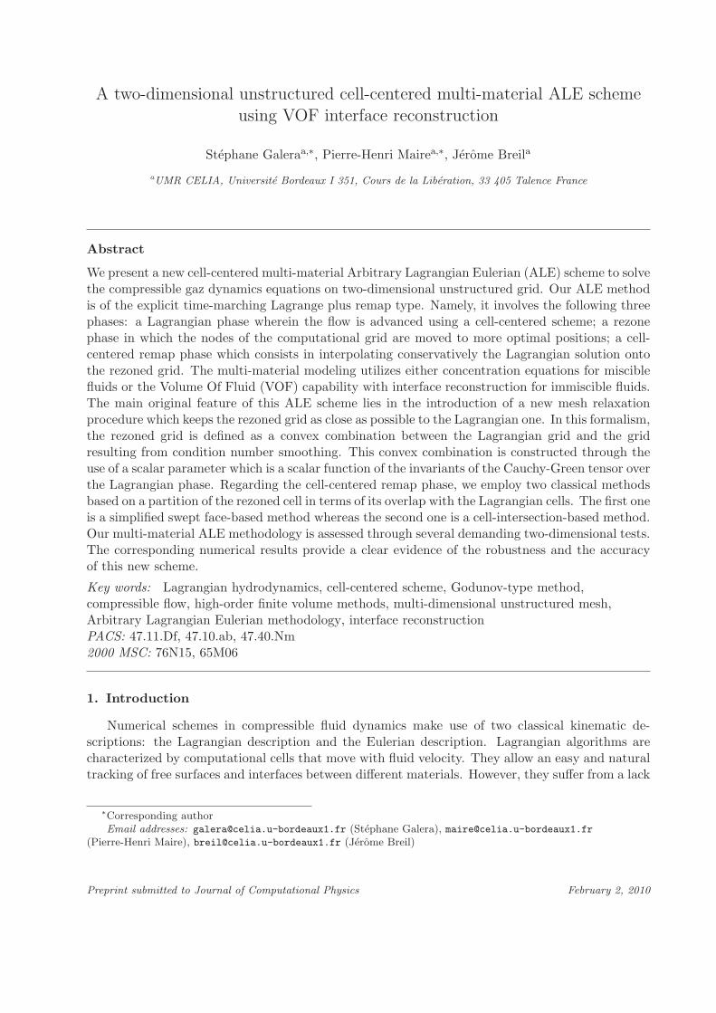
Figure 2: Fragment of a Lagrangian: notations related to a polygonal cell.

where V (t) is the Lagrangian (material) control volume, S(t) is its surface, and the time rates ofchange refer to quantities associated with this volume. In this case, the local kinematic equationis written

d

dtX = U , X(0) = x. (4)

In what follows, we recall briefly the cell-centered Lagrangian scheme which has been derived in[36]. Let us point out that this cell-centered scheme is compatible with the GCL in the sensethat nodal velocity and numerical fluxes are computed consistently by means of a node-centeredsolver. Moreover, this scheme is conservative and satisfies an entropy inequality in its first-ordersemi-discrete form. Before proceeding further, let us introduce some specific notations. Let c bea collection of non-overlapping polygons whose union covers the domain filled by the fluid. Eachcell is labeled with a unique index c and is denoted by Ωc. We denote by p the set of all thevertices of the cells. Each vertex is labeled with a unique index p. If we consider a given cell c,we introduce the set of all vertices of the cell c and denote it by P(c). For a given node p, wealso define the set of all cells that share this vertex and denote it by C(p). The sets P(c) and C(p)are counterclockwise ordered. For a node p ∈ P(c), p− and p+ are the previous/next nodes withrespect to p in the list of vertices of cell c, see Fig. 2. We denote by L−

pc and L+pc the half length

of the edges [p−, p] and [p, p+]. We use the same notation to define the unit normal outward N−pc

and N+pc, refer to Fig. 2. We also introduce the corner normal LpcNpc defined by

LpcNpc = L−pcN

−pc + L+

pcN+pc,

knowing that N2pc = 1.

All fluid variables are assumed to be constant in cell c and we denote them by using subscriptc. Therefore, we obtain a spatial approximation which is first order accurate. The set of evolutionequations for the the discrete unknowns ( 1

ρc,U c, Ec) is written using the Lagrangian conservation

7

equations in control volume form applied to cell c

mcd

dt(

1

ρc)−

∑

p∈P(c)

LpcNpc ·Up = 0, (5a)

mcd

dtU c +

∑

p∈P(c)

(L−

pcΠ−pcN

−pc + L+

pcΠ+pcN

+pc

)= 0, (5b)

mcd

dtEc +

∑

p∈P(c)

(L−

pcΠ−pcN

−pc + L+

pcΠ+pcN

+pc

)·Up = 0. (5c)

The mesh motion is governed by the local kinematic equation, which in its discrete form at pointp writes

d

dtXp = Up, Xp(0) = xp, (6)

where Xp = (Xp, Yp)t denotes the coordinates of point p at time t > 0 and xp its initial position.

In the above equations, Up denotes the velocity of the point p and Π−pc, Π+

pc are nodal pressureslocated at point p. These pressures can be seen as nodal pressures viewed from cell c and relatedto the two edges impinging at node p, refer to Fig. 2. These nodal quantities are obtained throughthe use of a nodal solver which reads

Up = M−1p

∑

c∈C(p)

[LpcPcNpc + MpcU c] , (7a)

Pc −Π−pc = Z−

pc (Up −U c) ·N−pc, (7b)

Pc −Π+pc = Z+

pc (Up −U c) ·N+pc, (7c)

where Pc denotes the cell-centered pressure and Mpc, Mp are 2× 2 matrices which write

Mpc = Z−pcL

−pc(N

−pc ⊗N−

pc) + Z+pcL

+pc(N

+pc ⊗N+

pc), Mp =∑

c∈C(p)

Mpc.

Here, Z±pc stands for swept mass flux, which according to [13] can be expressed as

Z±pc = ρc

[ac + Γc | (Up −U c) ·N

±pc |],

where ac is the isentropic sound speed in cell c and Γc is a material dependent parameter, which isdefined by setting Γc = γc+1

2 in the case of a perfect gas.Let us remark that the Mpc matrices are symmetric positive definite, thus providing a Mp matrix

which is also symmetric positive definite and hence always invertible. We point out that equations(7b) and (7c) stands for Riemann invariants along the unit outward normal directions. Finally, weget a first-order cell-centered discretization of the Lagrangian hydrodynamics equations based ona node flux discretization. It is shown in [36], that this discretization leads to a conservative andentropy consistent scheme in which the fluxes and the mesh motion are computed in a compatibleway so that the GCL is exactly fulfilled at the discrete level.

The accuracy of the present scheme is improved thanks to a high-order extension which uses atwo-dimensional version of the generalized Riemann problem (GRP) methodology [7]. This high-order Lagrangian scheme is precisely described in [35].

8

4. Thermodynamical closures for multi-material flows

In this section we describe two different approaches to deal with thermodynamical closure inthe case of a multi-material flow. This closure is required since during the remapping phase of ourALE algorithm the different fluids will flow through the cell edges.

4.1. Multi-material modeling using concentration equations

In this approach, the multi-material fluid flow is viewed as multi-component fluid mixturewherein the k-th fluid is characterized by its mass fraction Ck, i.e. the ratio between the mass offluid k and the total mass of the mixture. We assume that any components are completely misciblefrom a continuum view point. This assumption applies to gases or materials at high temperatures,i.e. plasmas. During the Lagrangian phase, the concentration of each fluid evolves following thevery simple equation d

dtCk = 0, that is the concentration of each fluid remains constant during the

Lagrangian phase. Consequently, concentration stands for a passive scalar which allows to trace thelocation of each material inside the flow. We use a pressure-temperature equilibrium assumption toderive the multispecies thermodynamical closure model. Doing that, we obtain an effective equationof state for our multicomponent fluid mixture. We suppose that each fluid follows a gamma gaslaw, namely its pressure, Pk, and specific internal energy, εk, write as function of temperature Tk

Pk =R

Mk

ρkTk, εk =R

(γk − 1)Mk

Tk,

where R denotes the perfect gas constant, γk the polytropic index of fluid k and Mk its molarmass. The mixture EOS closure problem requires finding the equilibrium mixture pressure, P , andtemperature, T , such that the following properties hold

• Volume conservation: 1ρ

=K∑

k=1

Ck

ρk

.

• Energy conservation: ε =K∑

k=1

Ckεk.

• Pressure equilibrium: Pk = P,∀k = 1 · · ·K.

• Temperature equilibrium: Tk = T, ∀k = 1 · · ·K.

Here, K denotes the total number of fluids, ρ, ε are the density and the specific internal energyof the mixture and ρk, εk the density and specific internal energy of fluid k. The solution of theprevious set of equations allows to write the following effective mixture gamma gas law

P = (γ − 1)ρε,

where γ is the effective polytropic index of the mixture, which writes

γ = 1 +

K∑

k=1

Ck

Mk

K∑

k=1

Ck

(γk − 1)Mk

. (8)

9

4.2. Multi-material modeling using Volume Of Fluid capability

In this second approach, we assume that the materials are immiscible. The Volume Of Fluid(VOF) methodology introduces a Lagrangian tracking capability for material interfaces into ourALE algorithm. Thus, we have to deal with mixed cells that contain different materials. The mixedcell modeling is based on the knowledge of the volume fractions. Being given the volume of themixed cell, V , and the volume occupied by the k-th fluid, Vk, the corresponding volume fractionwrites φk = Vk

V. The main issue related to the mixed cell is to define its evolution during the

Lagrangian phase. Namely, knowing the total change of volume, momentum and energy how shouldthey be distributed between materials. This is done using a closure model that allows to computean effective thermodynamical state in the mixed cell as function of the thermodynamical statesof the materials and the volume fractions. Here, we briefly recall the closure model based on theassumption of equal strain rates [44]. As noticed by Benson [8], this assumption is clearly incorrect ifwe apply it to a mixture of air and steel for instance. However, in spite of this crude approximation,this simple model is rather robust and gives quite acceptable results. More sophisticated modelsbased on the physical assumption of pressure relaxation are also available [4, 45, 23].

Let us denote by mk the partial mass of material k in the mixed cell. The total mass, m, writesobviously m =

∑k mk. Using the definition of the volume fraction one gets

mk

m=

ρ

ρk

φk, (9)

where ρ and ρk denote the global and the partial density of mass in the mixed cell. The timedifferentiation of (9) gives

ρkdφk

dt= ρkφk

(1

ρ

dρ

dt−

1

ρk

dρk

dt

). (10)

Since by assumption the volumetric strain rate is equal for all materials, i.e. 1ρ

dρdt

= 1ρk

dρk

dt, we

conclude that during the Lagrangian phase the volume fraction of each material is constant

φn+1k = φn

k . (11)

We note that this equal strain assumption is consistent with the fact that the materials in the mixedcell have the same velocity field, U , which is nothing but the Lagrangian cell-centered velocity ofthe mixed cell.

At the end of the Lagrangian phase, being given the volume of the mixed cell, V n+1, and thevolume fractions φn+1

k , we update the partial densities as

ρn+1k =

mk

φn+1k V n+1

. (12)

Knowing the volume fractions and the partial pressures, Pk, it remains to determine the effectivepressure, P , in the mixed cell. To this end, we write the time variation of internal energy for eachmaterial using the Gibbs relation

ρkdεk

dt+ Pkρk

d

dt(

1

ρk

) = ρkTkdsk

dt. (13)

Here, Tk and sk denote the temperature and the specific entropy for material k. We multiply thisequation by φk, sum over all materials, use energy conservation (mε =

∑k mkεk) and apply the

equal strain assumption to get

ρdε

dt+∑

k

φkPkρd

dt(1

ρ) =

∑

k

φkρkTkdsk

dt.

10

The comparison of this relation and the effective Gibbs relation written for the mixture

ρdε

dt+ Pρ

d

dt(1

ρ) = ρT

ds

dt, (14)

allows to define the effective pressure as

P =∑

k

φkPk. (15)

We also define the effective sound speed, a, knowing the sound speed of each material, i.e. a2k =(

dPk

dρk

)

sk

. We differentiate (15), knowing that φk is constant and using the equal strain assumption

to get

a =

(∑

k

φkρ

ρk

a2k

) 1

2

. (16)

This effective sound speed is used in our node-centered Riemann solver to compute the numericalfluxes, refer to Eq. (7).

Finally, it remains to update the internal energy for each material. Since we are using aGodunov-type method to discretize Lagrangian hydrodynamics, internal energy is calculated asthe difference between the total energy of the zone and its kinetic energy. Namely, at the discretelevel, the mixed cell internal energy variation is written

m(εn+1 − εn) = m

[En+1 − En −

1

2(Un+1)2 − (Un)2

].

Knowing the effective internal energy variation, we compute the global heating over the mixed cellas

δQ = m(εn+1 − εn) + Pn(V n+1 − V n), (17)

we note that this global heating corresponds to the approximation of the Gibbs relation (14) writtenfor the mixed cell. We compute the partial internal energy variation for each material by makingthe assumption that the global heating is distributed over each material as

mk(εn+1k − εnk) + Pn

k (V n+1k − V n

k ) = φkδQ. (18)

Let us remark that this formulation conserves energy in the sense that∑

k mk(εn+1k − εnk) =

m(εn+1−εn), due to the definition of the effective pressure, i.e. PnV n =∑

k Pnk V

nk and PnV n+1 =∑

k Pnk V

n+1k . We also point out that this distribution of heating over the materials amounts to

prescribe at the continuum level ρkTkdsk

dt= ρT ds

dt. In other words, we apply an equal time rate of

volumetric heating for both the mixed cell and the materials.

5. Interface reconstruction

The method used to reconstruct the interface, is an extension to the case of general unstructuredpolygonal grid of the algorithm initially designed by Youngs [49] . The goal of the method is toperform a Piecewise Linear Interface Construction (PLIC) in each mixed-cell, being given thevolume fraction of each fluid. We make the fundamental assumption that each mixed-cell containstwo immiscible fluids. For a given cell Ωc, each fluid is characterized by its volume fraction φc,k, k =1, 2, which stands for the ratio between the volume occupied by the fluid and the total volume of

11

the cell. Obviously, φc,k satisfies 0 ≤ φc,k ≤ 1 and φc,1 + φc,2 = 1. We define the reference volumefraction by setting φref

c = φc,1. Knowing φrefc we construct the interface as one segment of straight

line cutting the mixed cell into two pure regions. This line is defined in each cell by the equation

N c ·X + dc = 0, (19)

where X stands for the position vector of a generic point located on the line, N c is the unitnormal vector to the line, and dc is the signed distance from the line to the origin of the Cartesianorthonormal frame (0, X, Y ).

The first step of the interface reconstruction consists in computing an approximate unit normalN c in each cell c. This normal is evaluated using the following formula

N c = −∇φc

‖∇φc‖.

Here ∇φc denotes the gradient of the volume fraction. Although φ is not a smooth function, wecompute its gradient using a least squares approach. In each cell c, we assume a piecewise linearrepresentation of the volume fraction by writting

φc(X) = φrefc + ∇φc · (X −Xc),

where ∇φc is the constant gradient of the volume fraction and Xc is the centroid of the cell. Thus,∇φc is obtained by solving the minimization problem

∇φc = argmin∑

d∈C(c)

[φref

d − φrefc −∇φc · (Xd −Xc)

]2.

Here, C(c) denotes the set of the neighbouring cells of cell c. It is well known that this methodleads only to a first-order reconstruction of the normal [15, 2].

The second step of the reconstruction consists in computing dc by locating the interface alongthe normal direction so that the volume cut by the interface coincides with the sub-cell volumecomputed using the reference volume fraction φref

c . Knowing the unit normal N c, the location ofthe moving interface is uniquely defined by the value of the parameter d. Hence, d being given, thecorresponding sub-cell volume fraction can be expressed as a continuous monotonic function of d,φc(d). Thus, dc is obtained by solving the equation

φc(d) = φrefc ,

which has always a unique solution, refer to [15, 2] for the details about the numerical implemen-tation.

6. Rezoning phase

The rezoning phase consists in moving the node of the Lagrangian grid to improve the geometricquality of the grid while keeping the rezoned grid as close as possible to the Lagrangian grid.This constraint must be taken into account to maintain the accuracy of the computation broughtby the Lagrangian phase. In fact, by requiring the rezoned grid to remain as close as possibleto the Lagrangian grid, we minimize the error of the remap phase, and we justify employing alocal remapper in which mass, momentum and energy are simply exchanged between neighboringcells. In what follows, we first describe our grid smoothing algorithm which is the conditionsmoothing algorithm introduced by Knupp [25] for mesh quality optimization. Then, we present agrid relaxation algorithm which intends to keep the rezoned grid in the vicinity of the Lagrangiangrid. This grid relaxation procedure represents the most original contribution of this paper.

12

cp

p−

p+

+

Figure 3: Fragment of a grid: notations for condition number smoothing.

6.1. Condition number smoothing

We describe the condition number smoothing (CNS) algorithm, which is an unstructured ex-tension related of the well known Winslow algorithm as it has been demonstrated in [27]. We makethe assumption that the input grid (the grid produced by the Lagrangian phase) is unfolded. Ifthe Lagrangian phase produces non valid cells then we use an untangling procedure [46]. We firstrecall the condition number smoothing algorithm for an internal node, then we present an originalextension to the case of nodes located on a boundary.

6.1.1. Internal node

Let c be a given cell of the Lagrangian grid, p ∈ P(c) a particular node of this cell and p−, p+

the previous and next nodes with respect to p in the counterclockwise list of the vertices of cell c,refer to Fig. 3. Let Jcp = [pp+ | pp−] be the 2× 2 Jacobian matrix associated with each corner ata vertex p of cell c. It is shown in [25] that the condition number of matrix Jcp in IR2 writes

κ(Jcp) =‖pp+‖2 + ‖pp−‖2

Acp, (20)

where Acp is the area of the triangle whose vertices are p−, p, p+. We note that κ is minimal for anisosceles rectangular triangle. With this condition number, we define the local objective functionassociated to node p

Fp(Xp) =∑

c∈C(p)

∑

q∈Vc(p)

κ(Jcq). (21)

Here Xp denotes the vector position of point p, C(p) is the set of cells that share node p and Vc(p)is the set of vertices of cell c that are connected to vertex p (including p itself). By summing thisfunctional over all grid nodes, we can also define a global objective function.

One very important feature that can be seen explicitly in the definition of κ(Jcp) is that thefunctional has a barrier, i.e., the value of the functional approaches infinity when the new gridcontains a non valid grid for which Acp = 0. This explains how the condition number smoothingproduces unfolded grids.

The rezoned position of node p, Xrezp , is determined by minimizing the local functional (21)

using the first step of a Newton algorithm

Xrezp = Xn+1,lag

p − H−1p (Xn+1,lag

p )∇Fp(Xn+1,lagp ), (22)

where Xn+1,lagp denotes the vector position of point p at the end of the Lagrangian phase and

Hp is the 2 × 2 Hessian matrix related to Fp. We note that the computation of the Hessian and

13

the gradient of the functional are performed using the coordinates of the points at the end of theLagrangian phase. We separately minimize each of the local objective functions and iterate overall the nodes. This approach is termed as Jacobi sweep minimization. Its main advantage liesin the fact that it does not depend on the vertex order and thus leads to a symmetry preservingalgorithm.

6.1.2. Boundary node

p+

p−

p

i

Xp(t)

Figure 4: Boundary node treatment: notations for the Bezier curve. p−, p and p+ are vertices located on theboundary. The second-order interpolation Bezier curve, Xp(t) is plotted in black.

Let p denotes a boundary node and p−, p+ its previous and next neighbors in the list of boundarynodes, refer to Fig. 4. To define the rezoned position of node p in a consistent manner with thecondition number smoothing algorithm, we first determine a piecewise parametric representationof the boundary. To this end we introduce the second-order interpolation Bezier curve

Xp(t) = (1− t)2Xp− + 2(1− t)tXi + t2Xp+ , t ∈ [0, 1] (23)

where Xi denotes the vector position of point i, which is a control point of the Bezier curve. Thiscontrol point is defined so that the Bezier curve passes through point p. Hence, for a given t0 ∈]0, 1[,Xi is computed by setting Xp(t0) = Xp, this leads to

Xi =Xp − (1− t0)

2Xp− − t20Xp+

2(1− t0)t0. (24)

The parameter t0 is usually defined by setting t0 = 12 . Using the parametric representation of the

boundary curve, we define the nodal objective functional related to node p by setting

fp(t) = Fp(Xp(t)), (25)

where Fp is the functional defined by (21). Using the chain rule we get

dfp

dt= ∇Fp ·

d

dtXp(t),

d2fp

dt2= Hp

d

dtXp(t) ·

d

dtXp(t) + ∇Fp ·

d2

dt2Xp(t).

Finally, to find the rezoned position of point p, it remains to minimize the real function fp(t). Tothis end, we perform one step of a Newton procedure to compute

trez = t0 −

dfp

dt(t0)

d2fp

dt2(t0)

. (26)

14

After checking that trez ∈ [0, 1] the vector position of the rezoned point is defined as Xrezp =

Xp(trez). We note that this boundary node treatment performs particularly well in the case of free

boundary condition.

6.2. Relaxation algorithm

The updated location of the node is defined by mean of a convex combination between its rezonedlocation obtained from the previous CNS method and its location at the end of the Lagrangianphase

Xn+1 = Xn+1,lag + ωp (Xrez −Xn+1,lag),

where ωp ∈ [0, 1] is a node-based coefficient computed as a function of the invariants of the rightCauchy-Green strain tensor, which is associated to the deformation of the Lagrangian grid over atime step. Let us briefly recall the definition of these tensors which are basic tools in the frameworkof continuum mechanics, refer to [9]. For sake of conciseness, let X0 and X1 denote the positionvector of a generic point associated to the Lagrangian grid at time tn and at time tn+1 = tn + ∆t.We assume that these two grids are valid, hence we can define a one to one map between these twoconfigurations of the flow by setting X1 = Ψ(X0,∆t). This map is characterized by its Jacobianmatrix

F =∂Ψ

∂X0 ,

which is also named the deformation gradient tensor and can be explicitly written in IR2 as

F =

∂X1

∂X0

∂X1

∂Y 0

∂Y 1

∂X0

∂Y 1

∂Y 0

,

where X0 = (X0, Y 0)t and X1 = (X1, Y 1)t. We also introduce the determinant of the Jacobianmatrix, J = det F, which is strictly positive since the grids are valid. The right Cauchy-Greenstrain tensor, C, is obtained by right-multiplying F by its transpose, C = FtF. In our case, C is a2 × 2 symmetric positive definite tensor. We notice that this tensor reduces to the unitary tensorin case of uniform translation or rotation. It admits two positive eigenvalues, which are denotedλ1 and λ2 with the convention λ1 ≤ λ2. These eigenvalues can be viewed as the rates of dilationin the eigenvectors directions of the transformation. The definition of the ωp factor as a

function of the invariants of the right Cauchy-Green tensor leads to mesh relaxation

procedure which satisfies the principle of Galilean invariance, that is either for a

uniform translation or a pure rotation the relaxed mesh coincides with the Lagrangian

one. It remains to construct a node-centered approximation of the Cauchy-Green tensor. To thisend we use the Nanson formula [9] which expresses the change of length between the two Lagrangianconfigurations labeled (0) and (1). This formula writes

J(F−1)tN0 dL0 = N1 dL1, (27)

where dL0 and dL1 are the length elements in the configurations (0) and (1) and N0, N1 theircorresponding unit outward normals. Let us consider a cell Ωc and one of its vertices p. As usual,we denote p− and p+ the previous and the next vertex to p in the counterclockwise list of verticesof cell c. We display in Fig. 5 the fragments of cell c related to point p for the two Lagrangianconfigurations (0) and (1). The vectors L0,−

pc N0,−pc , L0,+

pc N0,+pc and L1,−

pc N1,−pc , L1,+

pc N1,+pc are the half

15

Ω0c

Ω1c

X0p+

L0,−pc N

0,−pc

L1,+pc N

1,+pc

X0p

X0p−

X1p

X1p+

X1p−

L1,−pc N

1,−pc

L0,+pc N

0,+pc

Figure 5: Fragments of the Lagrangian grids: configuration (0) (left) and configuration (1) (right).

outward normals related to point p and cell c for the two configurations. The deformation gradienttensor for cell c at point p, Fpc, is locally defined by applying the Nanson formula as follows

KpcL0,−pc N0,−

pc = L1,−pc N1,−

pc , (28a)

KpcL0,+pc N0,+

pc = L1,+pc N1,+

pc . (28b)

Here, Kpc is a 2 × 2 tensor which approximates K = J(F−1)t. Hence, using this definition, thecomponents of Kpc are expressed as

Kpc =

(F

yypc −F yx

pc

−F xypc F xx

pc

).

By solving the 2× 2 linear system (28) we are able to compute the components of the deformationgradient tensor related to cell c at point p. Finally, to compute the components of the deformationgradient tensor centered at point p, Fp, we employ a least squares approach by minimizing thefunctional

L(F xxp , F xy

p , F yxp , F yy

p ) =1

2

∑

c∈C(p)

[(KpL

0,−pc N0,−

pc − L1,−pc N1,−

pc

)2+(KpL

0,+pc N0,+

pc − L1,+pc N1,+

pc

)2],

where C(p) denotes the set of cells that surround point p and Kp is the tensor whose componentsare

Kp =

(F

yyp −F yx

p

−F xyp F xx

p

).

The Cauchy-Green tensor is obtained by computing Cp = FtpFp. Knowing this symmetric positive

definite tensor at each node, we compute its real positive eigenvalues λ1,p, λ2,p and define ωp as

ωp = 1−αp − αmin

1− αmin, (29)

where αp =λ1,p

λ2,pand αmin = minp αp. We point out that for uniform translation or rotation

λ1,c = λ2,c = 1 and ωp = 0, therefore the motion of the nodes is purely Lagrangian and we fulfillthe material frame indifference requirement. For other cases, ωp smoothly varies between 0 and 1.

16

7. Remapping phase

The remapping phase corresponds to a conservative interpolation of the physical variables fromthe Lagrangian grid at time tn+1 onto the rezoned grid. Since we are using a Lagrangian schemewherein the placement of the variables is cell-centered, we are developing a cell-centered remappingphase. Let c and c be respectively collections of non overlapping polygons of the Lagrangianand the rezoned grids. In what follows, we denote all quantities related to the rezoned grid usingthe tilde accent. Let ψ be a physical variable of the flow defined on c by its piecewise constantrepresentation ψc. Being given ψc, we want to compute

ψec =1

V (c)

∫

ec

ψ dX. (30)

That is, knowing the mean value of ψ over each cell of the Lagrangian grid, we want to computeits mean value over each cell of the new rezoned grid. To obtain a sufficiently accurate remapping,we first compute a piecewise monotonic linear reconstruction of the variable ψ over the Lagrangiangrid. Namely, knowing the mean value ψc, we re-construct the piecewise linear function, ψc(X),over the Lagrangian cell c as follows

ψc(X) = ψc + (∇ψ)c(X −Xc).

Here, (∇ψ)c denotes the constant gradient of ψ within cell c, which is computed using a leastsquares approach. The monotonicity of this reconstruction is enforced by using the classical Barth-Jespersen slope limitation procedure [6]. We also note that this reconstruction preserves the meanvalue ψc provided that Xc is the centroid of cell c, i.e.

Xc =1

V (c)

∫

c

X dX.

In this section we are dealing with remapping methods based on a partition of the volume of therezoned cell in terms of its overlap with the Lagrangian cells. Following the methodology derivedin [39] we have developed two approaches for the remapping phase that are briefly recall in thenewt two paragraphs.

7.1. Swept face-based method

Here, we briefly present an unstructured extension of the swept integration method presentedin [39]. Assuming a fixed topology between the old (Lagrangian) and the new (rezoned) grids, ageneric cell of the new grid can be decomposed as

c = c ∪

⋃

d∈C(c)\c

(c ∩ d)

\

⋃

ed∈C(ec)\ec

(c ∩ d)

. (31)

This decomposition, which is displayed in Fig. 6 (left), allows to write the mean value of ψ overthe new cell as

ψec =1

V (c)

∫

c

ψ dX +∑

d∈C(c)\c

∫

ec∩d

ψ dX −∑

ed∈C(ec)\ec

∫

c∩ed

ψ dX

.

Here, the volume of the new cell, V (c), is expressed as the volume of the old cell, plus the summationof the signed volumes of the quadrangular regions swept during the displacement of the edges, from

17

⋃d∈C(c)\c

(c ∩ d)

⋃

d∈C(c)\c

(c ∩ d)

cc

c

p

p+

p

c c+

Spp+

c p+

Figure 6: Decomposition of a rezoned cell (left). Swept region resulting from nodes displacement (right).

their old positions to their new ones. More precisely, each displacement of two consecutive verticesp and p+, leads to construct the quadrangular swept region Sp,p+ = p, p, p+, p+ whose volume isdenoted V (Sp,p+), refer to Fig. 6 (right). Using this notation, one obtains

V (c) = V (c) +∑

p,p+∈c

V (Sp,p+).

Following this approach, the mean value of ψ over the new cell writes

ψec =1

V (c)

∫

c

ψ dX +∑

p,p+∈c

∫

Sp,p+

ψ dX

.

The integral corresponding to the second term in the right-hand side, is the quadrangular sweptregion contribution to the flux. This integral is approximated in an upwind manner by setting

∫

Sp,p+

ψ dX =

∫S

p,p+ψc+(X) dX if V (Sp,p+) ≥ 0,

∫S

p,p+ψc(X) dX if V (Sp,p+) < 0,

(32)

where ψc+(X) and ψc(X) are piecewise linear reconstruction of the function ψ over the Lagrangiancells c+ and c.

7.2. Cell-intersection-based method

This approach is used when we are dealing with an old and a new grids whose connectivitiesdiffer. This situation occurs in the vicinity of mixed cells in the case of a multi-material computationusing VOF capability for interface tracking. For each rezoned cell, we need to compute exactlyits overlap with the surrounding Lagrangian cells. To this end, we employ an exact intersectionalgorithm which is based on a triangulation of the old and the new grids. Let us describe thedifferent steps of this algorithm.

1. Triangulation We perform the triangulation of the Lagrangian and the rezoned grid whichare initially paved with non overlaping polygonal cells. The triangulation of a convex polygonis a trivial operation by simply adding edges from one vertex to all other vertices as it displayed

18

in Fig. 7 (left). In the case of a non-convex polygonal cell, one way to triangulate it is byusing the assertion that any simple polygon without holes has at least two so called ’ears’. Anear is a triangle with two sides on the edge of the polygon and the other one completely insideit. The algorithm then consists of finding such an ear, removing it from the polygon (whichresults in a new polygon that still meets the conditions) and repeating until there is only onetriangle left. This algorithm is easy to implement and is known as ear clipping algorithm [16].The triangulation of a non-convex polygon using this algorithm is displayed in Fig. 7 (right).Being given a generic Lagrangian cell c and generic rezoned cell c, let us denote T (c) and T (c)their corresponding sets of triangles.

p

p−p+

T1

T2

T3 T4T5

T6

Figure 7: Triangulation of a convex polygon (left). Triangulation of non-convex polygonal (right) using ear clipping.The algorithm starts at point p which is an ear.

2. Intersection Assuming that the rezoned cell c is located in the neighborhood of the Lagrangiancell c, we compute the intersection of each triangle of T (c) with the triangles of T (d) for d ∈ C(c)where C(c) is the set of the neighboring cells of cell c. For a given couple of triangles (T, T )in T (d) × T (c) with d ∈ C(c) the intersection algorithm proceeds as follows. First, usingthe barycentric coordinates, we determine successively the localization of the vertices of T (c)in T (d) and the localization of the vertices of T (d) in T (c). Second, we compute the edgesintersection between T (c) and T (d).

3. Sub-polygon reconstruction The triangle-triangle intersection phase leads to a list of pointsthat are the vertices of a convex sub-polygon which is displayed in Fig. 8. We re-order in acounterclockwise manner the list of the vertices of this sub-polygon.

T

T

T ∩ T PT∩T

Figure 8: Sub-polygon that results from triangle-triangle intersection

19

4. Integration phase Let P(T ∩ T ) be the set of the intersection sub-polygons between T andT . Finally, the mean value of ψ over the rezoned cell c is computed as

ψec =1

V (c)

∑

Q∈P( eT∩T )

∫

Q

ψc dX,

where the integrals over the sub-polygons are evaluated using the piecewise linear reconstruc-tion of ψ over the Lagrangian cell. In this computation, the integrals of linear function over asub-polygon are exactly computed by means of the Green formula [40].

7.3. Mixed cell remapping

Here, we give some details about the remapping of the physical variables in mixed cell when weare using the VOF algorithm. The volume fractions are reconstructed on the rezoned cell as

φec,k =1

V (c)

∑

Q∈Pk( eT∩T )

∫

Q

dX, (33)

where Pk(T ∩ T ) is the set of intersection sub-polygons, associated to the material k. The globalmass and density are computed as

mec =∑

k

mec,k, and ρec =∑

k

ρec,kφec,k.

Let ψ be a physical variable and ψk its associated partial variable, ψ is remapped as

ψec =1

mec

∑

k

mec,kψec,k,

The update of effective pressure and sound speed is performed as described in Sec. 4.

7.4. Concentrations remapping

When we are modeling the multi-material flow using concentration equations, we have to remapthem to consistently update the thermodynamic state of each cell. Namely, to use the multi-speciesEOS developed in Sec. 4, we need to remap the concentrations of the K fluids, from the Lagrangiangrid onto the rezoned one. To this end, we first compute the mass of fluid k in the Lagrangian cellc, mc,k =

∫cρCk dV . We note that mc =

∑Kk=1mc,k since by definition

∑Kk=1Cc,k = 1. Then, the

mass of each fluid is conservatively interpolated onto the rezoned grid using the swept face-basedmethod; its remapped value is refered as mec,k. At this point, we remark that

mec 6=K∑

k=1

mec,k,

this discrepancy comes from the fact that our second-order remapping does not preserve linearitydue to slope limiting. Hence, we define the new concentrations by setting Cec,k =

mec,k

mecand impose

the renormalization

Cec,k ←−Cec,k∑K

k=1Cec,k

so that∑K

k=1Cec,k = 1. We point out that this necessary renormalization does not affect the globalmass conservation.

20

8. Numerical results

All the numerical results presented in this section are performed in Cartesian geometry. Thematerials are characterized by a perfect gaz equation of state which writes P = (γ − 1)ρε whereγ stands for the polytropic index of the gaz. The ALE computations are performed using therelaxation procedure described in Sec. 6. This procedure is applied every time step.

8.1. Two-material Sod problem

0 0.1 0.2 0.3 0.4 0.5 0.6 0.7 0.8 0.9 1

0.2

0.3

0.4

0.5

0.6

0.7

0.8

0.9

1

X

ρ

VOF computationConcentration modelAnalytical

0 0.1 0.2 0.3 0.4 0.5 0.6 0.7 0.8 0.9 10

0.2

0.4

0.6

0.8

1

1.2

1.4

1.6

1.8

2

X

pres

sure

VOF computationConcentration modelAnalytical

Figure 9: Two-material Sod problem density (left) and pressure (right). VOF and concentration equations modelingversus analytical solution.

0 0.1 0.2 0.3 0.4 0.5 0.6 0.7 0.8 0.9 10

0.2

0.4

0.6

0.8

1

1.2

1.4

X

velo

city

VOF computationConcentration modelAnalytical

0 0.1 0.2 0.3 0.4 0.5 0.6 0.7 0.8 0.9 10.5

1

1.5

2

2.5

3

3.5

X

ε

VOF computationConcentration modelAnalytical

Figure 10: Two-material Sod problem velocity (left) and internal energy (right). VOF and concentration equationsmodeling versus analytical solution.

We consider the two-material variant of the one-dimensional Sod shock tube problem describedin [45]. As usual, the computational domain is [0, 1] with an interface initially located at x =0.5. The initial conditions for left material are (ρl, Pl,U l, γl) = (1, 2,0, 2) and (ρr, Pr,U r, γr) =(0.125, 0.1,0, 1.4) for the right material. We point out that this test case is a genuine two-material

21

0 0.2 0.4 0.6 0.8 1 1.20

0.2

0.4

0.6

0.8

1

1.2

Figure 11: Initial unstructured polygonal grid for the Sedov problem.

problems for an ALE simulation run since the polytropic index is different for the left and theright material. The initial grid is made of 100 uniform cells and the final time is tfinal = 0.2. Werun this problem with our multi-material ALE scheme in its Eulerian version (as Lagrange plusremap). The first computation is performed using VOF interface reconstruction and the secondone uses concentration equations. The numerical results against the analytical solution are plottedin Fig. 9 for density and pressure and in Fig. 10 for velocity and internal energy. With this levelof resolution, we observe a quite good agreement between the numerical and analytical solutions.As expected, the contact discontinuity obtained with the VOF interface reconstruction is sharperthan the one obtained using concentration equations. We also note that the pressure plateau isvery well rendered with both methods in the sense that no spurious oscillations are created at thecontact discontinuity.

8.2. Sedov problem

We consider the Sedov problem for a point-blast in a uniform medium with cylindrical symmetry.An exact solution based on self-similarity arguments is available, see for instance [24]. The initialconditions are characterized by (ρ0, P0,U0) = (1, 10−6,0) and the polytropic index is set equal to75 . We set an initial delta-function energy source at the origin prescribing the pressure in the cellcontaining the origin as follows

Por = (γ − 1)ρorE0Vor

,

where Vor denotes the volume of the cell that contains the origin and E0 is the total amount ofreleased energy. By choosing E0 = 0.244816, as it is suggested in [24], the solution consists of adiverging shock whose front is located at radius R = 1 at time t = 1. The peak density reachesthe value 6. We point out that this simple mono-material problem does not require ALE to berun until final time. However, we use this problem as a sanity test case to demonstrate not onlythe accuracy and the robustness of our Lagrangian and ALE schemes but also their ability tohandle real unstructured grids. We also want to assess the efficiency of the relaxation algorithm

22

procedure. We run this problem on a unstructured grid produced by a Voronoi tessellation thatcontains 775 polygonal cells, which is displayed in Fig. 11. Using the same initial grid, we have run aLagrangian computation and two ALE computations. The results for the density obtained in thesethree configurations are displayed in Fig. 12. The Lagrangian results on top show the accuracyof the Lagrangian scheme, the shock level and its location are very well rendered. The first ALEcomputation (middle) has been performed switching off the relaxation procedure by setting ωp = 1,refer to Sec. 6. In this particular case, we note that the grid has been completely smoothed, theshock wave has been smeared over several cells and the density peak is quite far from its theoreticalvalue. The solution is quite far from the Lagrangian solution. Moreover, we note that grid motionoccurs even in regions where the flow is at rest. This flaw is visible for cells whose radius is greaterthan one. These remarks show the drawback of an ALE strategy using a pure rezoning phasewithout any relaxation procedure. The second ALE computation (bottom) has been done usingour relaxation procedure in which the new grid is constructed by making a convex combinationbetween the Lagrangian grid and the rezoned grid. This convex combination is based on the useof the ωp factor which is evaluated using the invariant of the Cauchy-Green tensor. Using thisapproach, it is possible to keep the rezoned grid as close as possible to the Lagrangian grid. Weobserve in Fig.12 (bottom) that the results obtained with the relaxation procedure are quite closeto those obtained with the Lagrangian scheme.

8.3. Triple point problem

Here, we present a two-material problem which corresponds to a three states two-dimensionalRiemann problem in a rectangular domain displayed in Fig. 13. The three-material extension of thisproblem using the Moment-of-Fluid method has been presented in [30]. The computational domainΩ = [0, 7]× [0, 3] is split into the following three sub-domains Ω1 = [0, 1]× [0, 3], Ω2 = [1, 7]× [0, 1.5]and Ω3 = [1, 7] × [1.5, 3]. The sub-domain Ω1 contains a high-pressure high-density fluid whoseinitial state is (ρ1, P1,U1) = (1, 1,0). The sub-domain Ω2 contains a low-pressure high-densityfluid whose initial state is (ρ2, P2,U2) = (1, 0.1,0). The sub-domain Ω3 contains a low-pressurelow-density fluid whose initial state is (ρ3, P3,U3) = (0.125, 0.1,0). The sub-domains Ω1 and Ω3

are filled with the same material characterized by the polytropic index γ1 = γ3 = 1.5 whereas thesub-domain Ω2 is filled with a different material with γ2 = 1.4. The boundary conditions are wallboundary conditions. The final time of the simulation is tfinal = 5. The initial grid is paved with70× 30 square cells.

The triple point is the point T located at the intersection of the three sub-domains Ω1, Ω2

and Ω3, its coordinates are T = (1, 1.5)t. Let us describe the evolution of the initial discontinuityat later time. For a point located on the interface between sub-domains Ω1 and Ω2, sufficientlyfar from the triple point T , the initial discontinuity is solved by a systems of three waves whichconsists of a contact discontinuity, a rightward shock wave and leftward rarefaction wave. The samesituation occurs for a point located on the interface between sub-domains Ω1 and Ω3, sufficiently farfrom the triple point. We note also that the interface between sub-domains Ω2 and Ω3 correspondsto a contact discontinuity. In the vicinity of the triple point T the situation is more intricate,since all the aforementioned waves interact and lead to complex two-dimensional fluid flow. Wepoint out that the two rightward shock waves in sub-domains Ω2 and Ω3 propagate with differentspeeds due to the difference of the acoustic impedance between the two fluids. Since ρ3a3 < ρ2a2,where a2 and a3 denotes the sound speed in sub-domains Ω2 and Ω3, the Ω3 rightward shock wavepropagates faster than the Ω2 rightward shock wave. This creates a strong shear along the initialcontact discontinuity located at the interface between Ω2 and Ω3. This shear produces a Kelvin-Helmholtz instability and a vortex formation occurs. We notice that the Lagrangian computation

23

0 0.2 0.4 0.6 0.8 1 1.20

0.2

0.4

0.6

0.8

1

1.2

0.8

1.8

2.8

3.8

4.8

5.8

0 0.2 0.4 0.6 0.8 1 1.20

1

2

3

4

5

6

r

ρ

LagrangianAnalytical

0 0.2 0.4 0.6 0.8 1 1.20

0.2

0.4

0.6

0.8

1

1.2

0.0

0.7

1.4

2.1

2.8

3.5

0 0.2 0.4 0.6 0.8 1 1.20

1

2

3

4

5

6

r

ρ

Pure ALEAnalytical

0 0.2 0.4 0.6 0.8 1 1.20

0.2

0.4

0.6

0.8

1

1.2

0.3

1.3

2.3

3.3

4.3

5.3

0 0.2 0.4 0.6 0.8 1 1.20

1

2

3

4

5

6

r

ρ

ALE with relaxationAnalytical

Figure 12: Sedov problem at final time t = 1. From bottom to top, ALE computation with relaxation procedure,ALE computation with pure rezoning (ωp = 1) and Lagrangian computation. Left column: density map and grid,right column: density as a function of the radius of cell centers versus analytical solution.

24

X

Y

0

γ1 = 1.5

1

ρ1 = 1

P1 = 1

7

3

ρ3 = 0.125

P3 = 0.1

γ3 = 1.5

ρ2 = 1

P2 = 0.1

γ2 = 1.4

1.5T

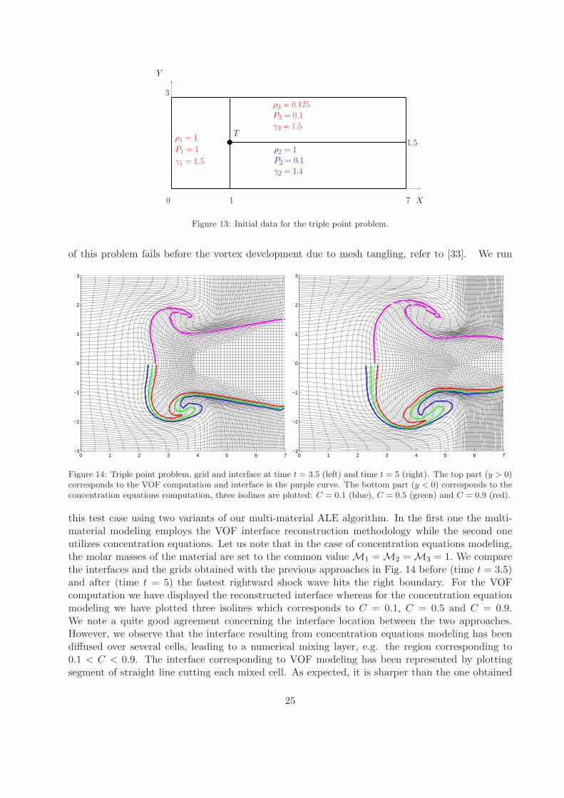
Figure 13: Initial data for the triple point problem.

of this problem fails before the vortex development due to mesh tangling, refer to [33]. We run

0 1 2 3 4 5 6 7−3

−2

−1

0

1

2

3

0 1 2 3 4 5 6 7−3

−2

−1

0

1

2

3

Figure 14: Triple point problem, grid and interface at time t = 3.5 (left) and time t = 5 (right). The top part (y > 0)corresponds to the VOF computation and interface is the purple curve. The bottom part (y < 0) corresponds to theconcentration equations computation, three isolines are plotted: C = 0.1 (blue), C = 0.5 (green) and C = 0.9 (red).

this test case using two variants of our multi-material ALE algorithm. In the first one the multi-material modeling employs the VOF interface reconstruction methodology while the second oneutilizes concentration equations. Let us note that in the case of concentration equations modeling,the molar masses of the material are set to the common value M1 =M2 =M3 = 1. We comparethe interfaces and the grids obtained with the previous approaches in Fig. 14 before (time t = 3.5)and after (time t = 5) the fastest rightward shock wave hits the right boundary. For the VOFcomputation we have displayed the reconstructed interface whereas for the concentration equationmodeling we have plotted three isolines which corresponds to C = 0.1, C = 0.5 and C = 0.9.We note a quite good agreement concerning the interface location between the two approaches.However, we observe that the interface resulting from concentration equations modeling has beendiffused over several cells, leading to a numerical mixing layer, e.g. the region corresponding to0.1 < C < 0.9. The interface corresponding to VOF modeling has been represented by plottingsegment of straight line cutting each mixed cell. As expected, it is sharper than the one obtained

25

0 1 2 3 4 5 6 7−3

−2

−1

0

1

2

3

0

0.17

0.34

0.51

0.68

0.85

0 1 2 3 4 5 6 7−3

−2

−1

0

1

2

3

1.7e−07

0.18

0.36

0.54

0.72

0.9

Figure 15: Triple point problem, map of ωp at time t = 3.5 (left) and time t = 5 (right). The top part (y > 0)corresponds to the VOF computation and the bottom part (y < 0) corresponds to the concentration equationscomputation.

0 1 2 3 4 5 6 7−3

−2

−1

0

1

2

3

0.25

0.74

1.2

1.7

2.2

2.7

0 1 2 3 4 5 6 7−3

−2

−1

0

1

2

3

0.25

0.77

1.3

1.8

2.3

2.8

Figure 16: Triple point problem, map of specific internal energy at time t = 3.5 (left) and time t = 5 (right). Thetop part (y > 0) corresponds to the VOF computation and the bottom part (y < 0) corresponds to the computationdone using concentration equations.

using concentration equations modeling. We have also displayed in Fig. 15, the ω parameter thatis used in the relaxation procedure. Let us recall that this parameter is computed as a function ofthe eigenvalues of the Cauchy-Green tensor, refer to Sec. 6. The maps of ωp are almost the samefor both computations. Moreover, we remark that this parameter is a good tracer that allows totrack the wave patterns. Indeed, the maxima of ωp are concentrated in regions where strong two-dimensional compressions occur. These regions of the flow are the locii where the maximum of meshsmoothing is taken into account. Finally, to track the shock waves and the contact discontinuity wehave plotted the specific internal energy map in Fig. 16. We observe quite similar results for bothapproaches, noticing that the vortex is little bit more diffused with the concentration equationsapproach.

26

8.4. Interaction of a shock wave with an Helium bubble

This test case corresponds to the interaction of shock wave with a cylindrical Helium bubblesurrounded by air at rest [43]. The initial domain is the rectangular box [0, L]×[−h

2 ,h2 ] = [0, 0.650]×

[−0.089, 0.089] displayed in Fig. 17. The cylindrical bubble is represented by a disk characterized byits center (xc, yc) = (0.320, 0) and its radius Rb = 0.025. We prescribe wall boundary conditions ateach boundary except at x = L, where we impose a piston-like boundary condition defined by theinward velocity V ⋆ = (u⋆, 0). The incident shock wave is defined by its Mach number, Ms = 1.22.The initial data for Helium are (ρ1, P1) = (0.182, 105), its molar mass is M1 = 5.269 10−3 and itspolytropic index is γ1 = 1.648. The initial data for air are (ρ2, P2) = (1, 105), its molar mass isM2 = 28.963 10−3 and its polytropic index is γ2 = 1.4. Using the Rankine-Hugoniot relations, wefind that the x-velocity of the piston is given by u⋆ = −124.824. The x-component of the incidentshock velocity isDc = −456.482. The incident shock wave hits the bubble at time ti = 668.153 10−6.The stopping time for our computation is tfinal = ti + 674 10−6 = 1342.153 10−6. It corresponds tothe time for which experimental shadow-graph extracted from [20] is displayed in [43].

To compute this problem, we have constructed two grids. The first one is a Cartesian gridthat contains 520× 144 = 74880 square cells. In this case, the initialization of the volume fractionis performed by computing the intersection between the circle, which corresponds to the bubbleboundary, and the Cartesian grid. Thus, we create mixed cells wherein the interface is representedby segment of straight line. The second grid is a polygonal grid that results from a Voronoitessellation wherein the boundary of the bubble is represented by faces of polygonal Voronoi cells,refer to [33] for more details about the construction of such a grid. This polygonal grid contains75507 cells which is approximately the same number of cells than the Cartesian grid. We notethat this initial polygonal grid does not contain any mixed cells. We have displayed these grids inFig. 18.

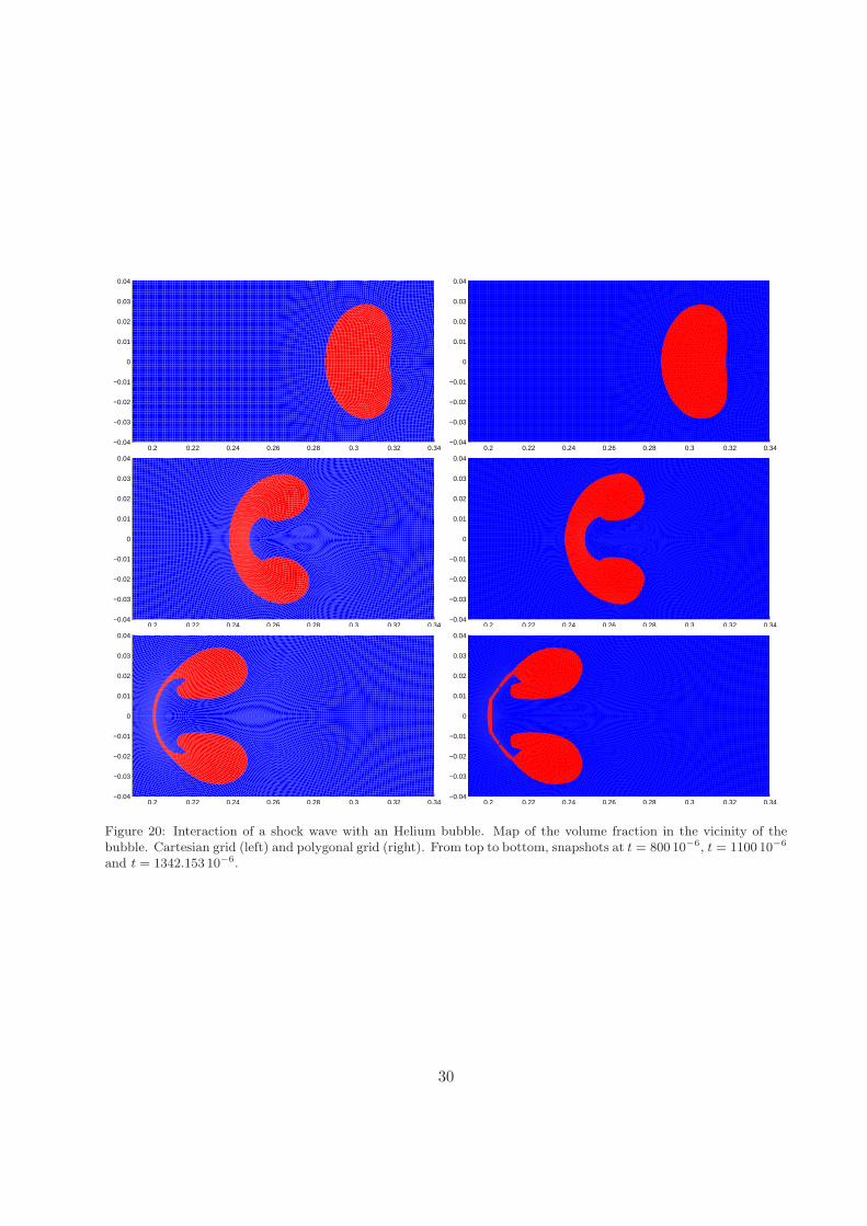
We have performed computations using VOF modeling for both grids with same grid relaxationprocedure. We have displayed in Fig. 20 for both grids the time evolution of the bubble. The firstsnapshot, located at the top of the figure, corresponds to time t = 800 10−6, after the interaction ofthe shock wave with the bubble. This interaction of the planar leftward shock wave with the curvedbubble interface leads to a transmitted shock and vortices formation. A complex system of wavesinteraction takes place, refer to [43] for a detailed analysis. At later times, t = 1100 10−6 (middle)and t = 1342.153 10−6 (bottom) the shape of bubble is strongly distorted. We note that the resultsobtained with both grids are quite similar. The comparison of an experimental Schlieren image[20] and the numerical results at the final time has been displayed in Fig. 19. It reveals a goodagreement that validates our ALE strategy from a qualitative point of view. It remains to performa quantitative validation using the numerical and experimental results presented in [43]. This willbe the topics of a future paper. Finally, to illustrate the relevancy of our relaxation parameter ωp,we have plotted it in Fig. 21, on a twice finer Cartesian grid at time t = 800 10−6. We clearly seenot only the fine structures of the interacting waves but also the shape of the bubble. This ωp

factor turns out to be a very relevant parameter to capture accurately the waves of the fluid flow.

8.5. Incompressible Rayleigh-Taylor instability

This test case deals with the well-known incompressible Rayleigh-Taylor instability. The com-putational domain is the rectangular box [0, 1

3 ] × [0, 1] which is paved with 34 × 100 cells. Theinitial set up consists of two immiscible fluids which are separated by a perturbed interface, whoseequation writes yi(x) = 1

2 + a0 cos(6πx). The interface amplitude a0 is set to the value a0 = 10−2.The heavy fluid is located above the light one. The densities of the two fluids are ρh = 2 andρl = 1. The same polytropic index γh = γl = 1.4 is shared by the two fluids. A downward gravity

27

0.295 0.3050.05

piston0.

178

Air HeFigure 17: Interaction of a shock wave with an Helium bubble. Geometry of the computational domain.

0.29 0.3 0.31 0.32 0.33 0.34 0.35 0.36−0.04

−0.03

−0.02

−0.01

0

0.01

0.02

0.03

0.04

0.29 0.3 0.31 0.32 0.33 0.34 0.35 0.36−0.04

−0.03

−0.02

−0.01

0

0.01

0.02

0.03

0.04

Figure 18: Interaction of a shock wave with an Helium bubble. Zoom on the initial grid in the vicinity of the bubbleand color map of volume fraction. Cartesian grid (left) and polygonal unstructured grid (right).

field is applied, g = (gx, gy)t = (0,−0.1)t. Initially both fluids are at rest and the initial pressure

distribution is deduced by setting hydrostatic equilibrium as

Ph(x, y) = 1 + ρhgy(y − 1), if y > yi(x),

Pl(x, y) = 1 + ρhgy[yi(x)− 1] + ρlgy[y − yi(x)], if y ≤ yi(x).

It is well known that this configuration is instable and as time evolves, the heavy fluid will sinkwhile the light fluid will rise. Due to the sinusoidal interface, vortices develop in the vicinity of theinterface and lead at later time to an interface which has a mushroom-like shape. Although thisproblem is incompressible and does not involve any shock wave, we run it using our multi-materialcompressible ALE algorithm using VOF modeling. The initial volume fractions are computed byperforming the intersection of the sinusoidal interface with the Cartesian grid. The computation isrun until the final time tfinal = 9. We have plotted in Fig. 22 the grid and interface at times t = 7,t = 8 and t = 9. We have also superimposed the interface obtained using the front tracking codeFronTier[19, 18]. The results of this code are used by the courtesy of J.W. Grove of the Los AlamosNational Laboratory. We point out that FronTier is run with a very fine resolution characterized

28

0.19 0.2 0.21 0.22 0.23 0.24 0.25 0.26−0.04

−0.03

−0.02

−0.01

0

0.01

0.02

0.03

0.04

0.19 0.2 0.21 0.22 0.23 0.24 0.25 0.26−0.04

−0.03

−0.02

−0.01

0

0.01

0.02

0.03

0.04

Figure 19: Interaction of a shock wave with an Helium bubble. Zoom on the bubble at tfinal = 1342.153 10−6 andcolor map of volume fraction. Cartesian grid on top left, polygonal grid on top right versus Schlieren image fromexperimental data [20](bottom).

by 106 × 320 cells. We note a rather good agreement between our results and Frontier interfacewhich shows the ability of our compressible ALE method to handle incompressible flows whereinstrong vorticity occurs.

8.6. Multi-mode implosion in cylindrical geometry

The aim of this test case is to assess the capability of our multi-material ALE algorithm to handlea multi-mode implosion in cylindrical geometry. This test problem which has been initially proposedin [50] is quite close to a real-life problem such as that encountered in Inertial Confinement Fusion

29

0.2 0.22 0.24 0.26 0.28 0.3 0.32 0.34−0.04

−0.03

−0.02

−0.01

0

0.01

0.02

0.03

0.04

0.2 0.22 0.24 0.26 0.28 0.3 0.32 0.34−0.04

−0.03

−0.02

−0.01

0

0.01

0.02

0.03

0.04

0.2 0.22 0.24 0.26 0.28 0.3 0.32 0.34−0.04

−0.03

−0.02

−0.01

0

0.01

0.02

0.03

0.04

0.2 0.22 0.24 0.26 0.28 0.3 0.32 0.34−0.04

−0.03

−0.02

−0.01

0

0.01

0.02

0.03

0.04

0.2 0.22 0.24 0.26 0.28 0.3 0.32 0.34−0.04

−0.03

−0.02

−0.01

0

0.01

0.02

0.03

0.04

0.2 0.22 0.24 0.26 0.28 0.3 0.32 0.34−0.04

−0.03

−0.02

−0.01

0

0.01

0.02

0.03

0.04

Figure 20: Interaction of a shock wave with an Helium bubble. Map of the volume fraction in the vicinity of thebubble. Cartesian grid (left) and polygonal grid (right). From top to bottom, snapshots at t = 800 10−6, t = 1100 10−6

and t = 1342.153 10−6.

30

Figure 21: Interaction of a shock wave with an Helium bubble. Map of ωp parameter in the vicinity of the bubblefor a twice finer Cartesian grid at t = 800 10−6. The red color indicates the maximum value, i.e. it shows the regionswhere the maximum deformation occurs.

(ICF) simulation. At the begining of the problem, a cylinder of light fluid (R ∈ [0, 1]) is surroundedby a shell of dense fluid (R ∈ [1, 1.2]), refer to Fig. 23. For both fluids the polytropic index isγl = γh = 5

3 . The initial densities and pressures are (ρl, Pl) = (0.05, 0.1) and (ρh, Ph) = (1, 0.1).The implosion is driven by prescribing the following pressure law on the outside of the dense shell

P ⋆(t) =

13, if t ∈ [0; 0.04],

13− 12.5 t−0.040.125−0.04 , if t ∈ [0.04; 0.125],

0.5, if t ∈ [0.125; 0.3].

(34)

We separate our study in two parts. The first one is devoted to the study of the one-dimensionalimplosion using two-dimensional grids. The second one consists in investigating the developmentof hydrodynamic instabilities which result from an initial multi-mode perturbation of the interfacebetween the light and heavy fluid.

8.6.1. One-dimensional implosion

The time history of the pressure driven implosion is displayed in Fig. 24 (left), using a classicalt − R diagram. This diagram is based on a one-dimensional Lagrangian computation. The one-dimensional grid is done using 50 equal size cells in the light fluid and 40 non-equal size cells inthe heavy fluid. The cells in the heavy fluid are graded according to a geometric progression toobtain a mass matching grid at the interface. The t − R diagram consists in plotting the radius

31

0 0.1 0.2 0.30

0.1

0.2

0.3

0.4

0.5

0.6

0.7

0.8

0.9

1

0 0.1 0.2 0.30

0.1

0.2

0.3

0.4

0.5

0.6

0.7

0.8

0.9

1

0 0.1 0.2 0.30

0.1

0.2

0.3

0.4

0.5

0.6

0.7

0.8

0.9

1

Figure 22: Incompressible Rayleigh-Taylor instability. Snapshots of the grid and map of the volume fraction at timest = 7, t = 8 and t = 9 versus FronTier interface (white curve).

P ⋆(t)

(ρh, Ph, γh) = (1; 0.1; 53)

(ρl, Pl, γl) = (0.05; 0.1; 53)

ri = 1

re = 1.2

Figure 23: One-dimensional implosion. Initial geometry and data.

32

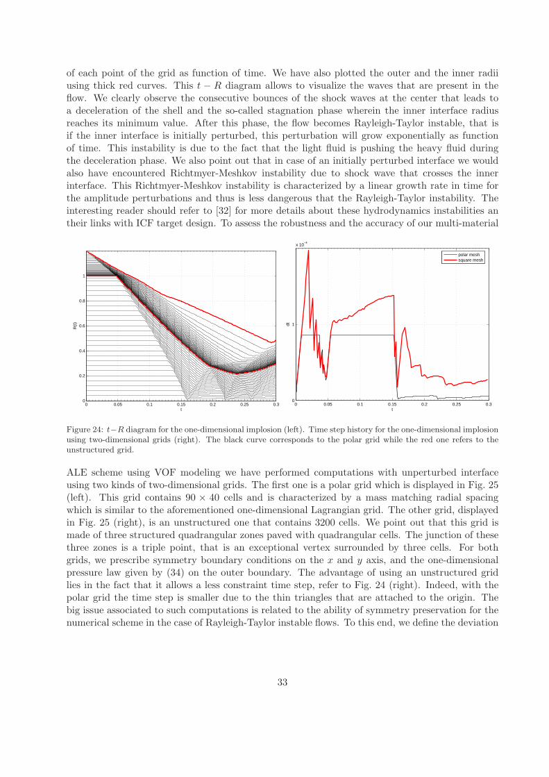
of each point of the grid as function of time. We have also plotted the outer and the inner radiiusing thick red curves. This t − R diagram allows to visualize the waves that are present in theflow. We clearly observe the consecutive bounces of the shock waves at the center that leads toa deceleration of the shell and the so-called stagnation phase wherein the inner interface radiusreaches its minimum value. After this phase, the flow becomes Rayleigh-Taylor instable, that isif the inner interface is initially perturbed, this perturbation will grow exponentially as functionof time. This instability is due to the fact that the light fluid is pushing the heavy fluid duringthe deceleration phase. We also point out that in case of an initially perturbed interface we wouldalso have encountered Richtmyer-Meshkov instability due to shock wave that crosses the innerinterface. This Richtmyer-Meshkov instability is characterized by a linear growth rate in time forthe amplitude perturbations and thus is less dangerous that the Rayleigh-Taylor instability. Theinteresting reader should refer to [32] for more details about these hydrodynamics instabilities antheir links with ICF target design. To assess the robustness and the accuracy of our multi-material

0 0.05 0.1 0.15 0.2 0.25 0.30

0.2

0.4

0.6

0.8

1

t

R(t

)

0 0.05 0.1 0.15 0.2 0.25 0.30

1

x 10−4

t

dt

polar meshsquare mesh

Figure 24: t−R diagram for the one-dimensional implosion (left). Time step history for the one-dimensional implosionusing two-dimensional grids (right). The black curve corresponds to the polar grid while the red one refers to theunstructured grid.

ALE scheme using VOF modeling we have performed computations with unperturbed interfaceusing two kinds of two-dimensional grids. The first one is a polar grid which is displayed in Fig. 25(left). This grid contains 90 × 40 cells and is characterized by a mass matching radial spacingwhich is similar to the aforementioned one-dimensional Lagrangian grid. The other grid, displayedin Fig. 25 (right), is an unstructured one that contains 3200 cells. We point out that this grid ismade of three structured quadrangular zones paved with quadrangular cells. The junction of thesethree zones is a triple point, that is an exceptional vertex surrounded by three cells. For bothgrids, we prescribe symmetry boundary conditions on the x and y axis, and the one-dimensionalpressure law given by (34) on the outer boundary. The advantage of using an unstructured gridlies in the fact that it allows a less constraint time step, refer to Fig. 24 (right). Indeed, with thepolar grid the time step is smaller due to the thin triangles that are attached to the origin. Thebig issue associated to such computations is related to the ability of symmetry preservation for thenumerical scheme in the case of Rayleigh-Taylor instable flows. To this end, we define the deviation

33

0 0.2 0.4 0.6 0.8 1 1.20

0.2

0.4

0.6

0.8

1

1.2

0 0.2 0.4 0.6 0.8 1 1.20

0.2

0.4

0.6

0.8

1

1.2

Figure 25: Initial grids for the one-dimensional implosion. Polar grid (left) and unstructured grid (right).

from symmetry preservation at the interface by introducing the following indicators

L∞(t) = maxi=1,...,41

| ri(t)− r(t) |,

L1(t) =1

41

41∑

i=1

| ri(t)− r(t) |,

L2(t) =

√√√√ 1

41

41∑

i=1

[ri(t)− r(t)]2.

Here, ri(t) denotes the radius of a vertex located on the interface and r(t) is the mean value of theinterface radius computed according to

r(t) =1

41

41∑

i=1

ri(t).

We have displayed in Fig. 26, these symmetry preservation indicators corresponding to a Lagrangian(left) and a multi-material ALE VOF (right) computations using the polar grid. As expected theLagrangian computation is correct since the maximum deviation from symmetry preservation isaround 4 10−7, which is a rather satisfying value. The values for the multi-material ALE VOFcomputation are a little bit bigger but remain still acceptable. We have also plotted the corre-sponding indicators in the case of the unstructured grid. For the Lagrangian computation, referto Fig. 27 (left), the maximum of symmetry preservation deviation is around 4 10−4. This highervalue is due to the non-symmetry of the initial unstructured grid. We observe that for the multi-material ALE VOF computation, refer to Fig. 27 (right), the symmetry preservation indicatorgrows to 1.5 10−3. We conclude that the symmetry preservation capability of our multi-materialALE VOF algorithm interface is directly comparable to the one of the Lagrangian method, whichcan be considered as a reference. The non-symmetric unstructured grid is clearly less stable than

34

the polar grid. However, we point out that we do not introduce spurious unstable mode that couldappear during the exponential growth of the Rayleigh-Taylor instability, refer to Fig. 28 where wehave displayed both grids at the final computation time.

0 0.05 0.1 0.15 0.2 0.25 0.30

0.5

1

1.5

2

2.5

3

3.5

4x 10

−7

t

∆ r

L∞L

1

L2

0.18 0.2 0.22 0.24 0.26 0.28 0.30

1

2

3

4

5

6x 10

−7

t∆

r

L∞L

1

L2

Figure 26: One-dimensional cylindrical implosion. Symmetry preservation indicators using a two-dimensional polargrid. Lagrangian computation (left) versus multi-material ALE computation using VOF modeling (right).

0 0.05 0.1 0.15 0.2 0.25 0.30

1

2

3

4

5

x 10−4

t

∆ r

L∞L

1

L2

0.18 0.2 0.22 0.24 0.26 0.28 0.30

0.5

1

1.5x 10

−3

t

∆ r

L∞L

1

L2

Figure 27: One-dimensional cylindrical implosion. Symmetry preservation indicators using a two-dimensional un-structured grid. Lagrangian computation (left) versus multi-material ALE computation using VOF modeling (right).

8.7. Two-dimensional implosion with perturbed interface

After investigating the capability of symmetry preservation of our multi-material ALE scheme,we are now ready to study the development of a compressible Rayleigh-Taylor instability. To thisend, we prescribe an initial perturbation at the interface between light and heavy fluid in thefollowing manner

rperti = ri [1 + a0 cos(nθ)] .

35

0 0.05 0.1 0.15 0.2 0.25 0.3 0.35 0.4 0.450

0.05

0.1

0.15

0.2

0.25

0.3

0.35

0.4

0.45

0 0.05 0.1 0.15 0.2 0.25 0.3 0.35 0.4 0.450

0.05

0.1

0.15

0.2

0.25

0.3

0.35

0.4

0.45

Figure 28: One-dimensional cylindrical implosion. Grids at final time for the multi-material ALE computation usingVOF modeling. Polar grid (left) and unstructured grid (right).

Here, ri and rperti denote the unperturbed and perturbed radii, a0 is the amplitude of the pertur-

bation and the integer n corresponds to the mode of the perturbation. We compute this problemusing the aforementioned two-dimensional grids for two different initial amplitudes a0 = 2 10−4 anda0 = 10−3 with the same mode n = 8.

The Lagrangian computations with a0 = 2 10−4 are displayed in Fig. 29 at the final timet = 0.3. We note that final grids remain valid for both initial grids. The Lagrangian computationscorresponding to a0 = 10−3 fails at tfail = 0.24 for both grids due to mesh tangling, refer to Fig. 30.This is not a surprise, as the higher the initial amplitude, the stronger the development of theRayleigh-Taylor instability.

Finally, we perform multi-material ALE VOF computations of this two-dimensional implosionwith perturbed interface. The final grids and the interfaces for the initial amplitude a0 = 2 10−4 areplotted in Fig. 31. We observe that the development of the instability is quite similar for both gridsand moreover is comparable to what has been obtained using Lagrangian computations, refer toFig. 29. Using the same framework, we have displayed the results obtained for the initial amplitudea0 = 10−3. Contrary to the Lagrangian computations, the multi-material ALE computations runwithout any problem up to the final time. We can observe, in Fig. 32, the same development ofthe interface instability for both initial grids. We also note that the time step corresponding to theinitial unstructured grid is much higher than the one corresponding to the initial polar grid, thusleading to a total computational time for the unstructured grid which is ten times smaller.

36

0 0.05 0.1 0.15 0.2 0.25 0.3 0.35 0.4 0.450

0.05

0.1

0.15

0.2

0.25

0.3

0.35

0.4

0.45

0 0.05 0.1 0.15 0.2 0.25 0.3 0.35 0.4 0.450

0.05

0.1

0.15

0.2

0.25

0.3

0.35

0.4

0.45

Figure 29: Two-dimensional implosion with perturbed interface. Lagrangian computation with a0 = 2 10−4. Gridsat final time, t = 0.3, corresponding to the initial polar grid (left) and the initial unstructured (right).

0 0.1 0.2 0.3 0.4 0.5 0.60

0.1

0.2

0.3

0.4

0.5

0.6

0 0.1 0.2 0.3 0.4 0.50

0.1

0.2

0.3

0.4

0.5

Figure 30: Two-dimensional implosion with perturbed interface. Lagrangian computation with a0 = 10−3. Grids atfailure time, tfail = 0.24, corresponding to the initial polar grid (left) and the initial unstructured (right).

37

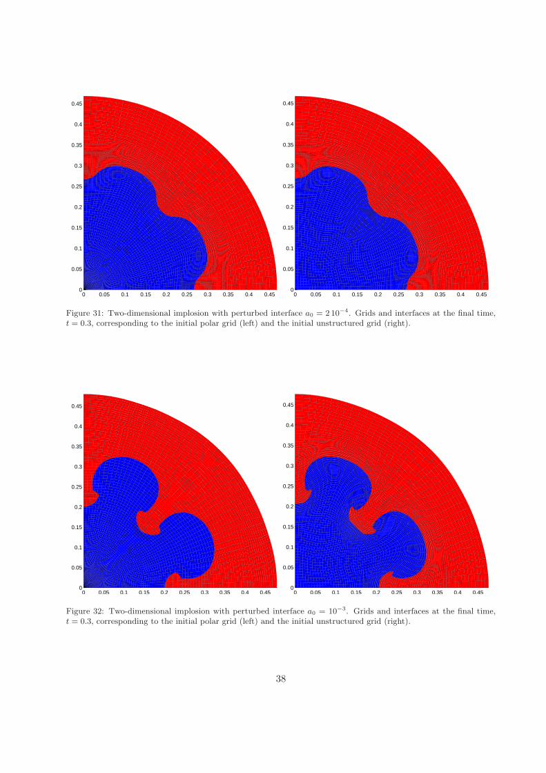
0 0.05 0.1 0.15 0.2 0.25 0.3 0.35 0.4 0.450

0.05

0.1

0.15

0.2

0.25

0.3

0.35

0.4

0.45

0 0.05 0.1 0.15 0.2 0.25 0.3 0.35 0.4 0.450

0.05

0.1

0.15

0.2

0.25

0.3

0.35

0.4

0.45

Figure 31: Two-dimensional implosion with perturbed interface a0 = 2 10−4. Grids and interfaces at the final time,t = 0.3, corresponding to the initial polar grid (left) and the initial unstructured grid (right).

0 0.05 0.1 0.15 0.2 0.25 0.3 0.35 0.4 0.450

0.05

0.1

0.15

0.2

0.25

0.3

0.35

0.4

0.45

0 0.05 0.1 0.15 0.2 0.25 0.3 0.35 0.4 0.450

0.05

0.1

0.15

0.2

0.25

0.3

0.35

0.4

0.45

Figure 32: Two-dimensional implosion with perturbed interface a0 = 10−3. Grids and interfaces at the final time,t = 0.3, corresponding to the initial polar grid (left) and the initial unstructured grid (right).

38

9. Conclusion

We have described a new high-order cell-centered ALE discretization devoted to the numericalsimulation of two-dimensional multi-material compressible fluid flows on general polygonal gridswith fixed topology. Our ALE algorithm includes the three following phases:

• An explicit Lagrangian phase wherein physical variables and the unstructured grid are up-dated by means of a recent cell-centered high-order Lagrangian scheme [35].

• An original rezoning phase in which the rezoned grid is defined as a convex combinationbetween the regularized grid and the Lagrangian grid. This convex combination is constructedthrough the use of an ω factor which is expressed in terms of the invariants of the right Cauchy-Green tensor with respect to the Lagrangian displacement over a time step. This relaxationprocedure is Galilean invariant and allows to keep the rezoned grid as close as possible to theLagrangian grid.

• A remapping phase in which physical variables are conservatively interpolated from the La-grangian grid onto the rezoned one.

Regarding the thermodynamical closure for multi-material flows, we have presented two differentapproaches. The first one, which corresponds to the case of miscible fluids, employs concentrationequations and a mixture EOS derived by assuming pressure-temperature equilibrium. The secondone, which corresponds to the case of immiscible fluids utilizes the Volume Of Fluid methodologyand allows a Lagrangian tracking capability for material interfaces in our ALE algorithm. In thisparticular approach, the mixed cell closure is obtained by means of the equal strain assumption.The numerical results that have been displayed demonstrate the accuracy and the robustness ofour ALE methodology in comparison to purely Lagrangian discretization.

At this point, we acknowledge that our ALE implementation is far from being optimal from thepoint of view of its capability, accuracy and efficiency. Concerning its capability and accuracy, weplan to improve the multi-material modeling in the case of immiscible fluids by implementing theMoment Of Fluid algorithm [2, 15]. This enhancement will allow to take into account more than two-materials and to reconstruct interfaces with a higher order of accuracy. We also plan to investigatethe implementation of more sophisticated mixed cell closure models such as pressure relaxationmodels [4, 23]. Concerning its efficiency, we intend to improve the remapping phase replacing thecostly exact intersection remapping algorithm by an hybrid remapping phase which is a combinationof the swept face-based and cell-intersection-based methods. In this hybrid remapping approach theuse of exact intersection remapping will be restricted to a buffer layer located in the vicinity of theinterfaces between materials. This hybrid method will be described in a forthcoming paper [17]. Wealso intend to improve our grid relaxation procedure. First, we think that it is possible to enhancethe smoothing algorithm by incorporating some physical weight into it. Second, we plan to includemore physics into the ω parameter definition to better take into account shear and vorticity usingthe polar decomposition of the right Cauchy-Green tensor [26]. Finally, to demonstrate the abilityof our method on more realistic problems, in a next paper, we will provide its two-dimensionalextension to axisymmetric geometry.

Acknowledgment

The authors thank M. Kucharik, R. Liska, R. Loubere, B. Rebourcet, M. Shashkov and P.Vachal for many fruitful and stimulating discussions about Lagrangian hydrodynamics and multi-

39

material ALE. The authors are also grateful to J. Grove from the Los Alamos National Laboratoryfor providing us the Frontier results and allowing their use.

References

[1] F. L. Adessio, D. E. Carroll, K. K. Dukowicz, J. N. Johnson, B. A. Kashiwa, M. E. Maltrud,and H. M. Ruppel. Caveat: a computer code for fluid dynamics problems with large distortionand internal slip. Technical Report LA-10613-MS, Los Alamos National Laboratory, 1986.

[2] H.T. Ahn and M.J. Shashkov. Multi-material interface reconstruction on generalized polyhe-dral meshes. J. Comput. Phys., 226(2):2096–2132, 2007.

[3] H.R. Anbarlooei and K. Mazaheri. Moment of fluid interface reconstruction method in multi-material arbitrary Lagrangian-Eulerian (MMALE) algorithms. Comput. Methods Appl. Mech.Engrg., 198:3782–3794, 2009.

[4] A. Barlow. A new Lagrangian scheme for multimaterial cells. In Proceedings of EuropeanCongress on Computational Methods in Applied Sciences and Engineering, ECCOMAS Com-putational Fluid Dynamics Conference, Swansea, Wales, pages 262–297, 2001.

[5] A.J. Barlow. A compatible finite element multi-material ALE hydrodynamics algorithm. Int.J. Numer. Meth. Fluids, 56(8):953–964, 2008.

[6] T. J. Barth and D. C. Jespersen. The design and application of upwind schemes on unstruc-tured meshes. In AIAA paper 89-0366, 27th Aerospace Sciences Meeting, Reno, Nevada, 1989.

[7] M. Ben-Artzi and J. Falcovitz. Generalized Riemann problems in computational fluids dynam-ics. Cambridge University press, 2003.

[8] D. J. Benson. Computational methods in Lagrangian and Eulerian hydrocodes. Comp. Meth.in Appl. Mech. and Eng., 99:235–394, 1992.

[9] J. Botsis and M. Deville. Mecanique des milieux continus : une introduction. Presses Poly-techniques et Universitaires Romandes, 2006.

[10] E.J. Caramana, D.E. Burton, M.J. Shashkov, and P.P. Whalen. The construction of compatiblehydrodynamics algorithms utilizing conservation of total energy. J. Comput. Phys., 146:227–262, 1998.

[11] B. Despres and C. Mazeran. Lagrangian gas dynamics in two dimensions and Lagrangiansystems. Arch. Rational Mech. Anal., 178:327–372, 2005.

[12] J. Donea, A. Huerta, J.-Ph. Ponthot, and A. Rodriguez-Ferran. Encyclopedia of ComputationalMechanics, volume 1: Fundamentals. John Wiley and Sons, 2004. Chapter 14: ArbitraryLagrangian-Eulerian methods.

[13] J. K. Dukowicz. A general, non-iterative Riemann solver for Godunov’s method. J. Comput.Phys., 61:119–137, 1984.

[14] J.K. Dukowicz, M.C. Cline, and F.S. Addessio. A general topology method. J. Comput. Phys.,82:29–63, 1989.

40

[15] V. Dyadechko and M. Shashkov. Reconstruction of multi-material interface from moment data.J. Comput. Phys., 227(11):5361–5384, 2008.

[16] D. Eberly. Triangulation by ear clipping. Geometric Tools, LLC, 2008. Available at http:

//www.geometrictools.com/Documentation/TriangulationByEarClipping.pdf.

[17] S. Galera, M. Kucharik, P.-H. Maire, M. Shashkov, M. Berndt, and J. Breil. Hybrid Remapping(Conservative Interpolation) for Multimaterial Arbitrary Lagrangian-Eulerian Methods. to besubmitted to Journal of Computational Physics, 2010.

[18] J. Glimm, J.W. Grove, X.L. Li, W. Oh, and D.H. Sharp. A critical analysis of Rayleigh-Taylorgrowth rates. J. Comput. Phys., 169:652–677, 2001.

[19] J. Glimm, J.W. Grove, X.L. Li, K.M. Shyue, Q. Zhang, and Y. Zeng. Three dimensional fronttracking. SIAM J. Scien. Comp., 19:703–727, 1998.

[20] J.F. Haas and B. Sturtevant. Interaction of weak-shock waves. J. Fluid Mech., 181:41–76,1987.

[21] C.W. Hirt, A. Amsden, and J.L. Cook. An arbitrary Lagrangian–Eulerian computing methodfor all flow speeds. J. Comput. Phys., 14:227–253, 1974.

[22] P. Hoch. An arbitrary lagrangian eulerian strategy to solve compressible fluid flows. HAL :hal-00366858, version 1, 2009. Available at http://hal.archives-ouvertes.fr/docs/00/

36/68/58/PDF/ale2d.pdf.

[23] J.R. Kamm and M. Shashkov. A pressure relaxation closure model for one-dimensional, two-material Lagrangian hydrodynamics based one the Riemann problem. Technical Report LA-UR-09-00659, Los Alamos National Laboratory, 2009.

[24] J.R. Kamm and F.X. Timmes. On efficient generation of numerically robust Sedov solutions.Technical Report LA-UR-07-2849, Los Alamos National Laboratory, 2007.

[25] P. Knupp. Achieving finite element mesh quality via optimization of the Jacobian matrix normand associated quantities. Part I – a framework for surface mesh optimization. Int. J. Numer.Meth. Engng., 48:401–420, 2000.

[26] P. Knupp. Algebraic mesh quality metrics. SIAM J. Scien. Comp., 23(1):193–218, 2001.

[27] P. Knupp, L. G. Margolin, and M. J. Shashkov. Reference Jacobian optimization-based rezonestrategies for arbitrary Lagrangian Eulerian methods. J. Comput. Phys., 176:93–128, 2002.

[28] P. Knupp and S. Steinberg. Fundamentals of Grid Generation. CRC Press, Boca Raton, 1993.

[29] P.M. Knupp. Achieving finite element mesh quality via optimization of the Jacobian matrixnorm and associated quantities. Part I - a framework for surface mesh optimization. Int. J.Numer. Meth. Engng., 48(3):401–420, 2000.

[30] M. Kucharik, R.V. Garimella, S.P. Schofield, and M.J. Shashkov. A comparative study of inter-face reconstruction methods for multi-material ale simulations. J. Comput. Phys., 229(7):2432–2452, 2009.

41

[31] M. Kucharik and M. Shashkov. Extension of efficient, swept-integration-based conservativeremapping method for meshes with changing connectivity. Int. J. Numer. Meth. Fluids,56(8):1359–1365, 2008.

[32] J. D. Lindl. Inertial Confinement Fusion. Springer, 1998.

[33] R. Loubere, P.-H. Maire, M. Shashkov, J. Breil, and S. Galera. Reale: A Reconnection-based Arbitrary-Lagrangian-Eulerian Method. Technical Report LA-UR-09-07844, Los AlamosNational Laboratory, 2009. submitted to J. Comput. Phys.

[34] H. Luo, J.D. Baum, and R. Lohner. On the computation of multi-material flows using ALEformulation. J. Comput. Phys., 194:304–328, 2004.

[35] P.-H. Maire. A high-order cell-centered Lagrangian scheme for two-dimensional compressiblefluid flows on unstructured meshes. J. Comput. Phys., 228:2391–2425, 2009.

[36] P.-H. Maire, R. Abgrall, J. Breil, and J. Ovadia. A cell-centered Lagrangian scheme forcompressible flow problems. SIAM J. Scien. Comp., 29(4):1781–1824, 2007.

[37] P.-H. Maire, J. Breil, and S. Galera. A cell-centered arbitrary Lagrangian-Eulerian (ALE)method. Int. J. Numer. Meth. Fluids, 56:1161–1166, 2008.

[38] L.G. Margolin. Introduction to ”An arbitrary Lagrangian-Eulerian computing method for allflow speeds”. J. Comput. Phys., 135(2):198–202, 1997.

[39] L.G. Margolin and M. Shashkov. Second-order sign-preserving remapping on general grids. J.Comput. Phys., 184:266–298, 2003.

[40] B. Mirtich. Fast and Accurate Computation of Polygonal Mass Properties. Journal of GraphicsTools, 1:31–50, 1996.

[41] J.M. Morrell, P.K. Sweby, and A. Barlow. A cell by cell anisotropic adaptive mesh ALE schemefor the numerical solution of the Euler equations. J. Comp. Phys., pages 1152–1180, 2007.

[42] B. Nkonga. On the conservative and accurate CFD approximations for moving meshes andmoving boundaries. Comput. Methods Appl. Mech. Eng., 190(13-14):1801–1825, 2000.

[43] James J. Quirk and S. Karni. On the dynamics of a shock-bubble interaction. Journal of FluidMechanics, 318:129–163, 1996.

[44] B. Rebourcet. Modelisations numeriques multifluides et multiphases - liens de principe. Tech-nical Report DO 119, CEA, 2006.

[45] M. Shashkov. Closure models for multimaterial cells in Arbitrary Lagragian Eulerian hy-drocodes. Int. J. Numer. Meth. Fluids, 56:1497–1504, 2008.

[46] P. Vachal, R. V. Garimella, and M. J. Shashkov. Untangling of 2D meshes in ALE simulations.J. Comput. Phys., 196:627–644, 2004.

[47] A.M. Winslow. Equipotential zoning of two-dimensional meshes. Technical Report UCRL-7312, Lawrence Livermore National Laboratory, 1963.

[48] A.M. Winslow. Numerical solution of the quasilinear poisson equation in a nonuniform trianglemesh. J. Comput. Phys., 1(2):149–172, 1966. Reprinted in 135(2):128–138, 1997.

42

[49] D.L. Youngs. Time dependent multi-material flow with large fluid distortion. In K.W. Mortonand M.J. Baines, editors, Numerical Methods for Fluid Dynamics, pages 273–285. AcademicPress, New York, 1982.

[50] D.L. Youngs. Multi-mode implosion in cylindrical 3d geometry. In 11th International Workshopon the Physics of Compressible Turbulent Mixing (IWPCTM11), Santa Fe, 2008.

43