A TWO-DIMENSIONAL STOCHASTIC MODEL FOR … Two-Dimensional Stochastic... · 2.3 Film Formation and...

A TWO-DIMENSIONAL STOCHASTIC MODEL FOR PREDICTION OF LOCALIZED CORROSION

A thesis presented to

the faculty of the

Russ College of Engineering and Technology of Ohio University

In partial fulfillment

of the requirements for the degree

Master of Science

Ying Xiao

November 2004

This thesis entitled

A TWO-DIMENSIONAL STOCHASTIC MODEL FOR PREDICTION OF LOCALIZED CORROSION

by

Ying Xiao

has been approved for

the Department of Chemical Engineering

and the Russ College of Engineering and Technology by

Srdjan Nesic

Professor of Chemical Engineering

Dennis Irwin

Dean, Russ College of Engineering and Technology

XIAO, YING. M.S. November 2004. CHEMICAL ENGINEERING

A TWO-DIMENSIONAL STOCHASTIC MODEL FOR PREDICTION OF

LOCALIZED CORROSION (71pp)

Director of Thesis: Srdjan Nesic

The two-dimensional (2-D) stochastic model, which describes the balance of two

processes: corrosion (leading to metal loss) and precipitation (leading to metal protection),

is able to predict localized corrosion, which is the most serious type of corrosion attack

found in practice. The model uses uniform corrosion rate and surface-scaling tendency

predicted by a 1-D mechanistic corrosion model as the inputs and can predict the

possibility of localized corrosion as a function of primitive parameters such as

temperature, pH, partial pressure of CO2, velocity, etc. The maximum penetration rate as

well as uniform corrosion rate can be predicted and used to describe the severity of the

localized attack.

Approved:

Srdjan Nesic

Professor of Chemical Engineering

ACKNOWLEDGEMENTS

I want to thank all the individuals who helped me complete this thesis. Although I

cannot list them all within this small page, I do want to express my deepest gratitude to

some of them directly involved in my research.

I would like to sincerely thank my advisor, Prof. Srdjan Nesic, for his guidance,

support and encouragement. His insight and knowledge in corrosion were the greatest

benefits to this work.

Many sincere thanks are due to my thesis committee members, Professor Daniel

Gulino, and Professor Dusan Sormaz, for their time, instructions, and patience during my

research.

I am pleased to acknowledge the support from Dr. Bert. M. Pots, for his sharing

the initial idea of this project and help to publish the work at NACE.

I am also greatly thankful to Mr. Herold for his instructions when I was writing

my thesis. This thesis could not be finished without his knowledge, and support.

Finally, special thanks to my husband, Dong Liu, my parents and sister for their

support and encouragement all of these years.

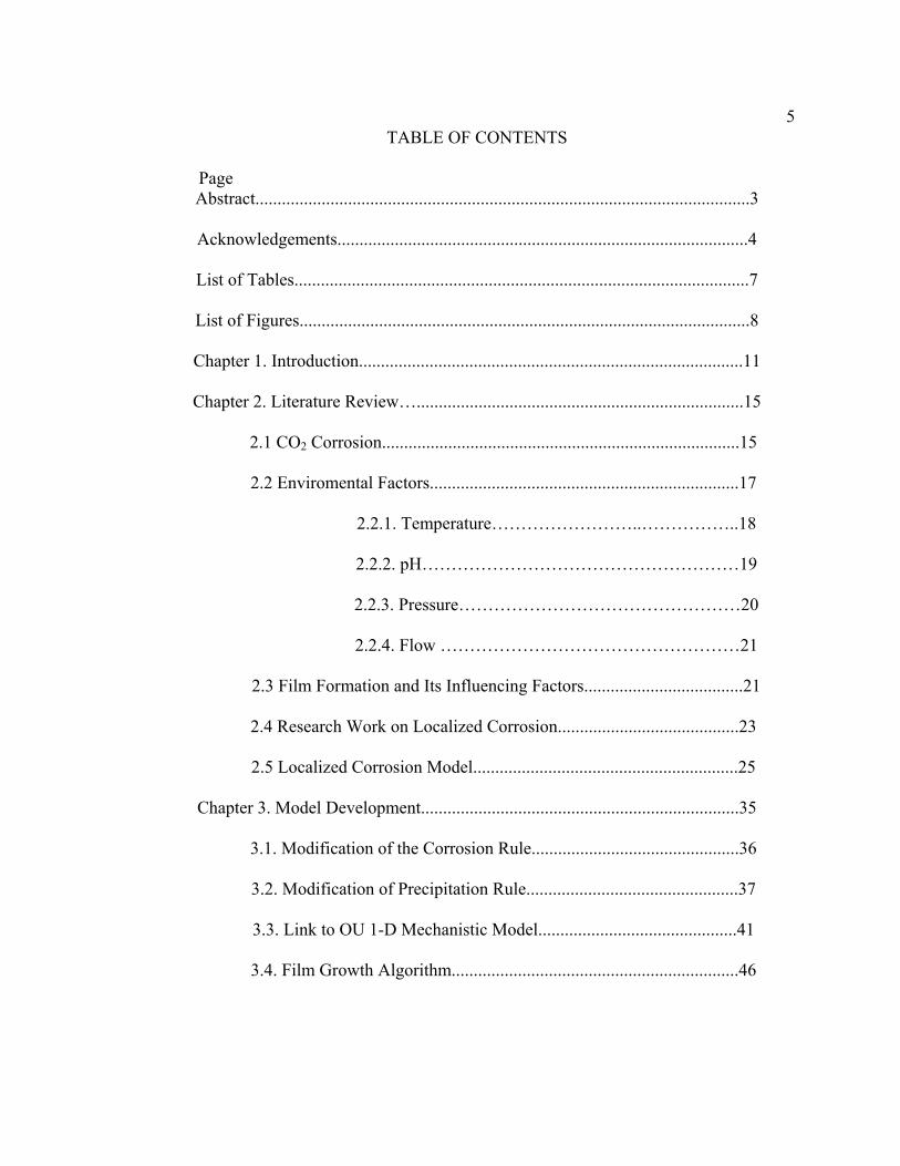
5TABLE OF CONTENTS

Page

Abstract................................................................................................................3

Acknowledgements.............................................................................................4

List of Tables.......................................................................................................7

List of Figures......................................................................................................8

Chapter 1. Introduction.......................................................................................11

Chapter 2. Literature Review…..........................................................................15

2.1 CO2 Corrosion.................................................................................15

2.2 Enviromental Factors......................................................................17

2.2.1. Temperature……………………..……………..18

2.2.2. pH………………………………………………19

2.2.3. Pressure…………………………………………20

2.2.4. Flow ……………………………………………21

2.3 Film Formation and Its Influencing Factors....................................21

2.4 Research Work on Localized Corrosion.........................................23

2.5 Localized Corrosion Model............................................................25

Chapter 3. Model Development........................................................................35

3.1. Modification of the Corrosion Rule...............................................36

3.2. Modification of Precipitation Rule................................................37

3.3. Link to OU 1-D Mechanistic Model.............................................41

3.4. Film Growth Algorithm.................................................................46

63.5. Implement a Path-Searching Algorithm to Remove Isolated

Islands…………………………………………………………………51

3.6. Localized Corrosion Tendency…………………………………...55

Chapter 4. Verification………………………………………………………...56

4.1 Comparison………………………..................................................56

4.2. Parameter Study…………………..................................................59

Chapter 5. Conclusions………………………………………………………..64

Chapter 6. Future Work……………………………………………………….65

References..........................................................................................................66

7

LIST OF TABLES Table Page

3.1. Test Matrix.................................................................................................................44

8

LIST OF FIGURES

Figure Page

Figure 1.1. Summary of natural gas transmission pipeline incidents by cause ................11

Figure 1.2. Corrosion accident categories in a major industry ………...…….………….13

Figure 2.1. The effect of pH on the solubility of iron carbonate at 2 bar pCO2, 40°C …..………...…………………………………………………………..20

Figure 2.2. Two samples of simulated metal surface morphology following rapid uniform corrosion without any film precipitation ……………………...……...…...…28

Figure 2.3. Two samples of the simulated metal surface morphology following rapid precipitation, which leads to a protective film and very little corrosion. ...…29

Figure 2.4. Two samples of simulated metal surface morphology following slow precipitation leading to an unprotective film and a moderate corrosion rate…………………………………………………………………………...30

Figure 2.5. Two samples of simulated metal surface morphology following moderate precipitation leading to a partially protective film and localized corrosion…31

Figure 3.1. Surface morphology prediction taken from the study of 2-D localized corrosion model by Nesic, Xiao, and Pots [2004]...........................................40

Figure 3.2. SEM images of the corroded steel surfaces taken from the study of CO2 corrosion in multiphase flow taken from the study by Nesic and Lunde [1994]………………………………………………………………….…….40

Figure 3.3. Predictions for the case of a 1%NaCl solution, at T = 80oC, pCO2 = 0.52bar, Ptotal = 1bar, CFe

2+ = 100ppm., v=1 m/s……………………………………...45

Figure 3.4 Film morphology taken from the proposed 2-D Model……………………...48

Figure 3.5 Film morphology and cross section of iron carbonate at pH 6.6, 80oC, 50ppm CFe

2+, stagnant flow………………………………………………………….48

Figure 3.6 Comparison of the film morphology before (top) and after (bottom) using a random film formation algorithm at pH 6.6, 80oC, 5ppm Fe2+ and 0.52bar pCO2………………………………………………………………………..…49

9Figure 3.7 Comparison of the film morphology at higher magnification before (top) and

after (bottom) using a random film formation algorithm at pH 6.6, 80oC, 5ppm Fe2+ and 0.52bar pCO2 ………………………………………………………..50

Figure 3.8 Comparison of the film morphology before (top) and after (bottom) using a random film formation algorithm at pH 6.5, 80oC, 50ppm Fe2+ and 0.52bar pCO2…………………………………………………………………………..51

Figure 3.9 Image for isolated islands taken from original Pots’ algorithm at ST=0.31………………………………………………………………………52

Figure 3.10. Comparison of the surface morphology, uniform corrosion rate and maximum penetration rate before (bottom) and after (top) implementing path-searching algorithm at pH 6.26, 80oC, 50ppm Fe2+ and 0.52bar pCO2…………………………………………………………………………..53



Figure 4.1. Comparison of uniform corrosion rate between 2-D prediction, 1-D prediction and experimental at pH 6.0, 80oC, 0.52bar pCO2, 50ppm Fe2+, rpm=0…………………………………………………………………….…..57

Figure 4.2. Comparison of film morphology between 2-D prediction, 1-D prediction and experimental at pH 6.0, 80oC, 0.52bar pCO2, 50ppm Fe2+, rpm=0…………...57

Figure 4.3. Comparison of uniform corrosion rate between 2-D prediction, 1-D prediction and experimental at pH 6.3, 80oC, 0.52bar pCO2, 50ppm Fe2+, rpm=0………………………………………………………………………...58

Figure 4.4. Comparison of film morphology between 2-D prediction, 1-D prediction and experimental at pH 6.3, 80oC, 0.52bar pCO2, 50ppm Fe2+, rpm=0………..…58

Figure 4.5. Comparison of uniform corrosion rate between 2-D prediction, 1-D prediction and experimental at pH 6.6, 80oC, 0.52bar pCO2, 50ppm Fe2+,rpm=0……..…………………………………………………………....59

Figure 4.6. Comparison of film morphology between 2-D prediction, 1-D prediction and experimental at pH 6.6, 80oC, 0.52bar pCO2, 50ppm Fe2+, rpm=0…….........59

10Figure 4.7 Film morphology and corresponding corrosion rate predicted by 2-D model at

0.54bar pCO2, 0ppm Fe2+, 80 °C, pH 6.6,1m/s……………………………….61

Figure 4.8 Film morphology and corresponding corrosion rate predicted by 2-D model at 0.54bar p , 5ppm Fe , 80 °C, pH 6.6,1m/s………………………….........61 CO2

2+

Figure 4.9 Film morphology and corresponding corrosion rate predicted by 2-D model at 0.54bar pCO2, 10ppm Fe2+, 80 °C, pH 6.6,1m/s……………………………...61

Figure 4.10 Film morphology and corresponding corrosion rate predicted by 2-D model at 0.54bar pCO2, 25ppm Fe2+, 80 °C, pH 6.6, 1m/s…………………………..62

Figure 4.11 Film morphology and corresponding corrosion rate predicted by 2-D model at 0.54bar pCO2, 28ppm Fe2+, 80 °C, pH 6.6,1m/s……………...….……...62

Figure 4.12 Film morphology and corresponding corrosion rate predicted by 2-D model at 0.54bar pCO2, 30ppm Fe2+, 80 °C, pH 6.6, 1m/s………………….…….63

Figure 4.13 Film morphology and corresponding corrosion rate predicted by 2-D model at 0.54bar pCO2, 50ppm Fe2+, 80 °C, pH 6.6, 1m/s………………….…….63

11

CHAPTER 1

INTRODUCTION

Carbon and low alloy steel are the principal construction materials for natural gas

pipelines due to their advantages in economy, availability and strength. It is estimated

that carbon and low alloy steel comprise 99% of materials used in the oil industry.

Although there have been many developments in corrosion resistant alloys over the past

few decades, carbon and low alloy steel are the most cost effective options. Usually

these materials are three to five times cheaper than stainless steel.

Natural Gas Transmission Pipeline

Incident Summary by Cause 1/1/2002 - 12/31/2003

Reported Cause Number of Incidents

% of Total Incidents

Property Damages

% of Total Damages

Fatalities Injuries

Excavation Damage 32 17.8 $4,583,379 6.9 2 3

Natural Force Damage 12 6.7 $8,278,011 12.5 0 0

Other Outside Force Damage 16 8.9 $4,688,717 7.1 0 3

Corrosion 46 25.6 $24,273,051 36.6 0 0

Equipment 12 6.7 $5,337,364 8.0 0 5

Materials 36 20.0 $12,130,558 18.3 0 0

Operation 6 3.3 $2,286,455 3.4 0 2

Other 20 11.1 $4,773,647 7.2 0 0

Total 180 $66,351,182 2 13

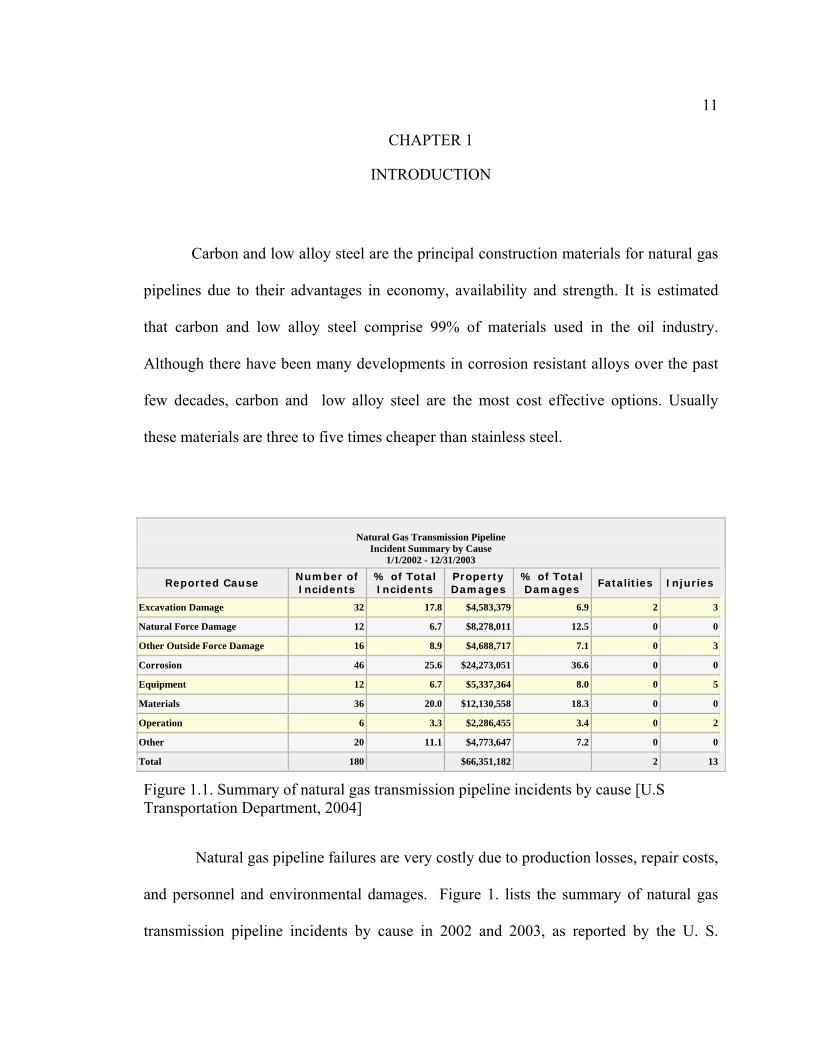
Figure 1.1. Summary of natural gas transmission pipeline incidents by cause [U.S Transportation Department, 2004]

Natural gas pipeline failures are very costly due to production losses, repair costs,

and personnel and environmental damages. Figure 1. lists the summary of natural gas

transmission pipeline incidents by cause in 2002 and 2003, as reported by the U. S.

12Department of Transportation Research and Special Programs Administration, Office of

Pipeline Safety (RSPA/OPS) [U.S Transportation Department, 2004]. It demonstrates

that corrosion (internal and external) is the most common cause of natural gas

transmission pipeline incidents, accounting for around 25% of all the incidents in 2002-

2003. In certain circumstances, internal corrosion comprises almost 50% of all incidents

(Alberta 1998).

Low-alloy steel pipeline carrying natural gas from well heads to treatment units

can be subject to corrosion caused by carbonic acid formed from carbon dioxide and

water often present as impurities in the produced streams. Carbon dioxide corrosion, also

called “sweet corrosion”, is by far the most prevalent form of internal corrosion

encountered in oil and gas production. It is getting more and more attention in recent

years with the fast development of modern oil and sweet gas recovery techniques.

The internal corrosion failures are generally not caused by uniform corrosion, but

rather by localized corrosion such as pitting and/or flow induced localized corrosion

(FILC). In order to run the oil and gas pipelines under safe and reliable conditions, it is

important to predict the amount of internal corrosion that occurs before significant

damage occurs. When it comes to monitoring, a number of electrochemical apparatus are

qualified to test the uniform corrosion; however there is not much progress in monitoring

localized corrosion. So, in practice, localized corrosion is the most serous and frequent

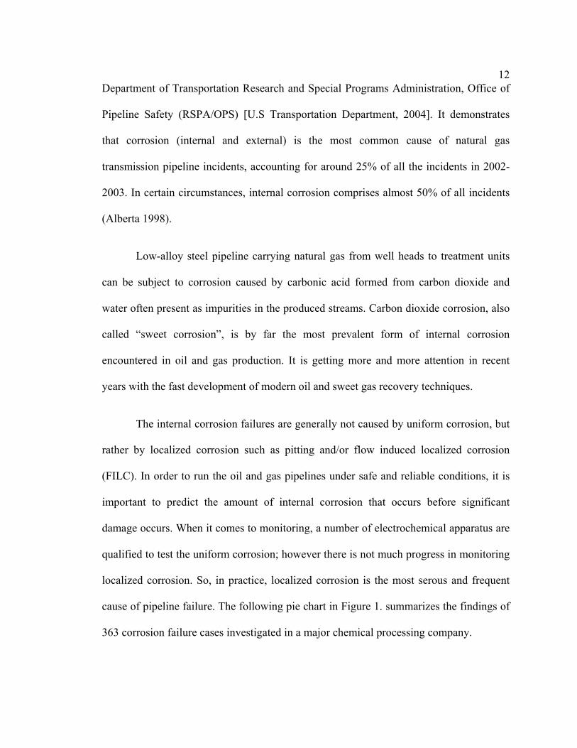
cause of pipeline failure. The following pie chart in Figure 1. summarizes the findings of

363 corrosion failure cases investigated in a major chemical processing company.

13

Figure 1.2 Corrosion accident categories in a major industry

The percentage of accidents, caused by the two types of localized corrosion,

pitting and crevice corrosion, is 22% and 12%, respectively. Stress corrosion cracking

(SCC), which is often initiated by pitting, accounts for 18%. So, the failures directly

caused by localized corrosion comprise 50% of the total accident. Currently, few

effective techniques are available for monitoring localized corrosion in an oilfield [Fu

1996]. Nearly all the generally used electrochemical techniques have some shortcomings

when detecting localized corrosion.

http://www.corrosion-doctors.org/Forms/scc.htm

14Due to the difficulty of monitoring localized attack, in this thesis, a stochastic

localized corrosion model considering film formation is proposed to predict the

occurrence of localized corrosion. The model has been calibrated with reliable

experimental data and its objective is to assist in safe pipeline design and/or operation.

15

( )

CHAPTER 2

LITERATURE REVIEW

The corrosion process is a physicochemical process, and the mechanism of carbon

steel corrosion in CO2 environment is extremely complex. Depending upon the system

conditions, either uniform or localized corrosion occurs. In recent decades, significant

attention has been paid to uniform corrosion and the mechanism of CO2 corrosion. Some

uniform corrosion models have been developed [Nordsveen 2003 and de Waard 1995].

However, relatively little attention has been given to localized corrosion. It is still not

well understood. A lot of research effort is needed before a full mechanism of localized

corrosion model is established.

2.1 CO2 Corrosion

A number of studies have been done under varying conditions of pressure,

temperature, pH value and water cut considering CO2 corrosion. The basic CO2 corrosion

reactions have been clearly understood and well accepted based on the work in the recent

decades. The major chemical reactions, include CO2 dissolution and hydration to form a

weak carbonic acid, are described as follows:

( )aqCOgCO ⇔

COHOHCO ⇔+

22 (2-1)

. (2-2) 3222

Then it dissociates into bicarbonate and carbonate ions through two steps:

16−+

−+− +⇔ 2

K

(2-3) +⇔ 332 HCOHCOH

. (2-4) 33 COHHCO

When the concentrations of Fe2+ and CO32- ions exceed the solubility limit ( ),

they combine with each other to form solid iron carbonate film (also called corrosion

product film) as follows:

sp

( )22 −+

K

−+2

−+

−−

sFeCOCOFe 33 ⇒+ . (2-5)

Here is a function of temperature and ionic strength. COsp 2 corrosion rates can be

reduced significantly when iron carbonate film precipitates on the surface of the steel.

The electrochemical reactions on the steel surface include the anodic reaction of

iron dissolution:

(2-6) +→ eFeFe 2

and two cathodic reactions. One of the reactions is the hydrogen evolution reaction:

. (2-7) 222 HeH →+

the other is direct reduction of carbonic acid:

(2-8) +→+ 3232 222 HCOHeCOH

17

2.2 Environmental Factors

Considering the basic reactions in CO2 corrosion shown above, one can appreciate

that a number of environmental factors, such as solution chemistry, flow velocity,

temperature, pressure, and pH value etc., can affect the uniform CO2 corrosion rate of

mild steel. Significant progress in recognition of the major parameters influencing

phenomenology and kinetics of the uniform corrosion of various steels in CO2 has been

achieved. But there still is no understanding of the exact mechanisms of processes

leading to the localized corrosion. Brossia [2000] suggested that the ratio of the chloride

concentration to the total carbonate concentration, solution pH, and solution temperature,

play critical roles in establishing conditions that promote localized corrosion, as well as

in influencing the rate of propagation at potentials above repassivation potential. He

concluded that there is no clear dependency of the severity or mode of attack on each

independent parameter and the initiation of pit seem to be of stochastic nature.

The oil industry’s experience with deep gas wells indicates that corrosion is not

severe at places where scale uniformly covers the surface of the tubing. Laboratory tests

have repeatedly demonstrated that a thin adherent layer of ferrous carbonate deposited on

the surface of a corroding material significantly reduces the corrosion rate. So, any

changes in the parameters that can increase precipitation kinetics (e.g. increasing iron

concentration, carbonate concentration, or temperature) might improve film adherence

under this scenario [Johnson 1991]. Corrosion rate is thus decreased by such strategies.

18The effect of the most important factors on CO2 corrosion are temperature, pH

value, pressure, solution composition, and flow, and each will be discussed separately.

2.2.1 Temperature

Temperature has major effects on corrosion. On one hand, higher temperature

increases reaction rates and transport of species, and hence results in a higher corrosion

rate. On the other hand, the increased temperature also accelerates the kinetics of

corrosion product precipitation. In CO2 solutions, the corrosion product, iron carbonate

precipitates and deposits on the metal surface after its solubility limit is reached. The rate

of ferrous carbonate precipitation is extremely temperature sensitive [Johnson 1991].

According to Johnson, at low temperatures, precipitation progresses more slowly than

corrosion reactions. At elevated temperatures, transport limited ferrous carbonate

deposition is theoretically limited by the corrosion reaction. Corroding surfaces may be

immediately passivated by FeCO3 precipitation at high temperature. At intermediate

temperatures, ferrous carbonate may drive the corrosion reaction by removing iron from

solution at approximately the same rate as it is provided by corrosion.

Dugstad et al. [1994] reported that increased corrosion rates with increasing

temperature in a single-phase flow reached a maximum corrosion rate between 60°C and

90°C. However, there is no research that reveals the effect of temperature on localized

corrosion.

192.2.2 pH

Since pH value indicates the concentration of protons in solution, which is one of

the major species involved in cathodic reaction of corrosion process, pH value of the

solution has been shown to play a dominant role in determining the corrosion mode of

carbon steels. High pH value decreases the H+ reduction rate of cathodic reaction due to

the insufficient protons in the solution, while low pH value enhances it. A correlation

between pH value and cathodic corrosion rate has been reported as

BpHAic +−=log (2-9)

where ic is the corrosion current, A is a positive number and B is a constant. Different

cathodic mechanism gave different A values [de Waard 1975, Nesic 1996].

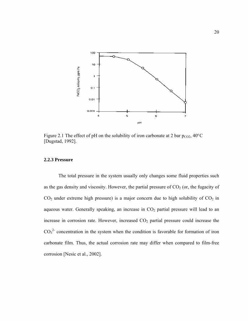
In addition to the effects on the electrochemical reaction rates, pH value also has a

dominant effect on the formation of iron carbonate films due to its effect on the solubility

of iron carbonate, as illustrated in Figure 2.1.

The figure shows that solubility of iron carbonate is reduced with the increase of

pH under this condition. Thus, if all the other conditions stay the same, a higher pH value

results in an increased saturation of iron carbonate. If the concentration of iron

concentration exceeds the saturation limit, iron carbonate scale forms and continuously

decreases the corrosion rate.

So, higher pH value decreases corrosion rate by reducing cathodic reaction and

forming scales.

20

Figure 2.1 The effect of pH on the solubility of iron carbonate at 2 bar pCO2, 40°C [Dugstad, 1992].

2.2.3 Pressure

The total pressure in the system usually only changes some fluid properties such

as the gas density and viscosity. However, the partial pressure of CO2 (or, the fugacity of

CO2 under extreme high pressure) is a major concern due to high solubility of CO2 in

aqueous water. Generally speaking, an increase in CO2 partial pressure will lead to an

increase in corrosion rate. However, increased CO2 partial pressure could increase the

CO32- concentration in the system when the condition is favorable for formation of iron

carbonate film. Thus, the actual corrosion rate may differ when compared to film-free

corrosion [Nesic et al., 2002].

212.2.4 Flow

Corrosion caused by fluid flow is usually called flow affected or flow accelerated

corrosion (FAC). Flow affects corrosion mainly through the mass transport process

involved in the corrosion mechanism. Generally speaking, higher flow rates are directly

associated with higher turbulence and more thorough mixing in the solution. It affects not

only the corrosion rate, but also the precipitation rate of iron carbonate [Nesic et al., 2002]

by bring more corrosive species onto the steel surface and corrosion products away from

the steel surface. Both effects contribute to less protective films being formed at higher

velocities. With extremely high velocities, flow can even mechanically remove corrosion

product films and can cause FILC, which is also called erosion corrosion.

Flow regime could be a very important factor for corrosion when multiphase flow

exists. Water being in contact with the steel surface is a prerequisite for CO2 corrosion.

For some flow regime, such as stratified or annular flow regime, water spreads on the

steel surface and causes corrosion. However, for some other flow regime, such as slug

flow regime, water could be all picked up by oil/gas and hence results in a low corrosion

rate. The severity of the CO2 corrosion attack is proportional to the time that the steel

surface is wetted by the water phase [Kermani and Smith, 1997]. The effect of the flow

regime can not be separated from the water/oil/gas ratio.

2.3 Film Formation and Its Influencing Factors

As we know, corrosion is usually not severe in the place where forms scale.

Laboratory tests illustrate that the major composition of the scale in CO2 corrosion is iron

22carbonate. The protective property of iron carbonate was obtained by offering greater

resistance to diffusion of species involved in the electrochemical reactions and/or by

simply blocking the reaction surface [Nesic and Lunde, 1994].

The precipitation kinetics of iron carbonate proposed by van Hunnik et al. [1996]

is as follows:

[ ] ( )( )12 11 −+ −−= SSKV

kFe sprprecA

(2-10)

where kr is a temperature-dependent rate constant, A/V is the ratio of metal surface area to

solution volume, and S is defined as

[ ][ ]spKCOFeS = 3

−+ 22

k

. (2-11)

Here Ksp is the solubility product of iron carbonate, which is a function of temperature

and solution ionic strength. Variables [Fe2+] and [CO32-] represent the equilibrium

concentrations of the solution.

According to (2-11), any changes of the parameters that increase precipitation

kinetics might improve film protectiveness [Johnson 1991], and hence decrease corrosion

rate. Protective iron carbonate films have been observed in systems with high Fe2+

concentrations, high PCO2, and high pH, which all lead to high S, and at high temperature,

which lead to high [Nesic 2003]. r

23The protectiveness of the scale is not only related to the precipitation kinetics, but

also related to the scale morphologies. Experimental data demonstrated [De Moraes et al.

2000] that a thin (less than 30 µm), compact and adherent layer of iron carbonate

deposited onto the surface of a corroding material significantly reduces the corrosion rate

when comparing to a thick (~100 µm) and porous scale. This highly protective scale was

present only with high temperature (93°C) and high pH (pH>5.0).

van Hunnik et al. [1996] proposed a so-called “scaling tendency” concept to

describe the protectiveness of the film. The scaling tendency is defined as the ratio of the

scale precipitation rate to the corrosion rate expressed in the same units. Obviously, when

ST << 1, the rapidly corroding metal surface opens voids under the film much faster than

precipitation can fill them out, which leads to porous and unprotective films. For instance,

at room temperature, little or no iron carbonate film forms even at high super saturations

as a result of the slow kinetics of the precipitation reaction. This effect is also attributable

to the fact that the metal surface “corrodes away” under the film. As ST exceeds 0.5,

conditions become favorable for formation of dense protective iron carbonate films.

2.4 Research Work on Localized Corrosion

Localized corrosion is the type of corrosion where an intense attack occurs at

localized sites on the metal surface while the rest of the surface corrodes at a much lower

rate, either because of an inherent property of the component material or because of some

environmental effect. For instance, if corrosion protection breaks down locally then

corrosion may be initiated at these local sites. Under such circumstances, it has been

24shown that the anodic surface area (Sa), where Fe will release its two electrons and

become Fe2+, is much smaller than the cathodic surface area (Sc), where the positive H+

ions usually will gain the electrons and become a H2. The small ratio of Sa/Sc can drive

corrosion to a higher rate by Fe trying to release sufficient electrons to be consumed at

the cathodic surface.

Some progress has been achieved in the recognition of major parameters

influencing phenomenology and kinetics of the uniform corrosion. But there is yet no full

understanding of the exact mechanisms of the processes leading to localized corrosion.

Flow induced localized corrosion (FILC) is a typical kind of localized corrosion.

Joosten [1994] initiated the experiments to observe and record the development of the

corrosion process under flowing conditions. His experiments laid a foundation for the

understanding of localized corrosion. The most common FILC is mesa attack. Nyborg

[1998] investigated initiation and growth of mesa attack by video recordings in flow loop

experiments performed at 80˚C and a pH value of 5.8. It is then proposed that a partially

protective corrosion film is a prerequisite for mesa attack.

Although flow is a crucial parameter to initiate localized corrosion, it is well

known that there are other environmental factors, such as pH, temperature, partial

pressure of CO2, Cl- concentration, material compositions, etc [Sun 2003] that cause

carbon steel to undergo a rapid localized corrosion process. Brossia [2000] studies some

parameters that influence the rate of propagation of pitting and he didn’t find a clear

dependency of the severity or mode of attack on each individual parameter. But he

concluded that the initiation of pit seems to have a stochastic nature.

25Sun and Nesic [2003] studied a number of factors that might influence localized

corrosion in wet gas flow, including pH, temperature, pressure, flow velocity, flow

regime, water cut and steel type. These studies confirmed Nyborg’s assumption that

partially protective film is a prerequisite for localized attack.

2.5 Localized corrosion model

Significant progress has been achieved in understanding uniform CO2 corrosion,

and hence some uniform corrosion models have been built successfully. However, far

less attention has been given to localized CO2 corrosion. It is not well understood yet, and

it is more difficult to predict or detect localized corrosion than uniform corrosion.

A FILC prediction model was proposed by Gunaltun [1996]. He applied a

turbulence factor to the general corrosion rate assuming the flow as being the main

parameter initiating localized attack.

In 1999, Schmitt developed a model for the prediction of flow induced localized

corrosion [1999]. The model correlates the hydrodynamic forces exerted onto corrosion

product scales with the fracture stress of the scales. The model is based on the assumption

that turbulence elements in the near-wall region of the turbulent boundary layer exchange

momentum with the wall and fatigue the corrosion product scale above critical wall shear

stresses [Schmitt 2000] . The author also claims that extrinsic stresses such as wall shear

stresses in flowing media are generally too small to contribute much to the local

destruction of scales [Schmitt 1996].

26Although flow is a very important factor to induce localized corrosion, it has been

proved that other parameters such as pH value, temperature, partial pressure of CO2, and

solution chemistry, can also induce and/or propagate localized corrosion. So, in this

thesis, a model taking into account all of these factors is proposed.

Localized corrosion of metals is a random process in nature [Williams 1984 and

1985, Wu 1997]. It is believed to be related to two random processes: the breakdown of

the passive film and the repassivation of the exposed area [Bertocci 1986, Hashimoto

1992, Stockert 1989, Pistdrius 1992, Gabrielli 1990, and Gabrielli 1992]. The

probabilistic character of localized attack makes a stochastic approach possible [Williams

1984 and 1985, Wu 1997]. The random (stochastic) process exhibits marked

deterministic features to form stable pitting due to the statistical results of a large number

of performances of these two processes [Hoerle 1998].

In 1996, Pots [van Hunnik and Pots 1996] wrote a two-dimensional (2-D)

stochastic algorithm to simulate the morphology of localized attack. The rule-based

algorithm is based on the assumption that the morphology of corrosion attack depends on

the balance of two processes: corrosion (leading to metal loss) and precipitation (leading

to metal protection). This balance has effectively been quantified by van Hunnik et al.

[1996] using a single parameter, the scaling tendency (ST),

CR

ST FeCO3=R

(2-12)

27Rwhere is the precipitation rate of iron carbonate and CR the corrosion rate. Both

are expressed in the same volumetric (e.g. mm/y) units. It has been experimentally

observed that if the precipitation rate overwhelms the corrosion rate, a protective film

forms onto the metal surface and the corrosion rate is greatly reduced. Correspondingly,

if the corrosion rate is much larger than the precipitation rate, protective films cannot be

formed since corrosion creates voids underneath the film faster than precipitation can fill

them up. According to a recent experimental study by Sun and Nesic [2003], there is a

“gray zone” between these extremes where localized corrosion occurs and the

corresponding scaling tendency is between 1 and 3.

3FeCO

For the original Pots’s [1996] algorithm, ST (ST has been defined above) is used

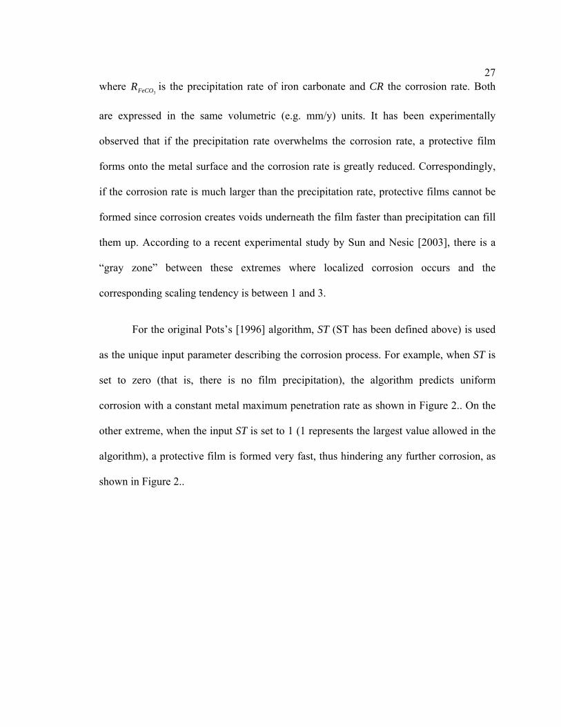
as the unique input parameter describing the corrosion process. For example, when ST is

set to zero (that is, there is no film precipitation), the algorithm predicts uniform

corrosion with a constant metal maximum penetration rate as shown in Figure 2.. On the

other extreme, when the input ST is set to 1 (1 represents the largest value allowed in the

algorithm), a protective film is formed very fast, thus hindering any further corrosion, as

shown in Figure 2..

28

Solution

Figure 2.2. Two samples of simulated metal surface morphology following rapid uniform corrosion without any film precipitation. Original Pots’s algorithm [1996] was used.

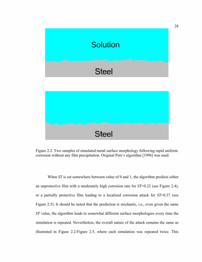
When ST is set somewhe

an unprotective film with a mod

or a partially protective film le

Figure 2.5). It should be noted t

ST value, the algorithm leads to

simulation is repeated. Neverthe

illustrated in Figure 2.2-Figure

re between value of 0 and 1, the algorithm predicts either

erately high corrosion rate for ST=0.22 (see Figure 2.4),

ading to a localized corrosion attack for ST=0.37 (see

hat the prediction is stochastic, i.e., even given the same

somewhat different surface morphologies every time the

less, the overall nature of the attack remains the same as

2.5, where each simulation was repeated twice. This

29property matches with the deterministic features in the stochastic pitting process reported

by Hoerle [1998]. This implied that the stochastic model can predict localized attack

repeatedly as long as the conditions are the same.

Protective film

Figure 2.3. Two samples of the simulated metal surface morphology following rapid precipitation, which leads to a protective film and very little corrosion. Original Pots’s [1996] algorithm was used.

It is remarkable that one can obtain all these various forms of corrosion attack by

varying a single parameter, the scaling tendency. Also interesting is the fact that the

algorithm captures the experimental behavior reported by Nyborg [1998] and Sun and

Nesic [2003] related to localized corrosion occurring in the “grey zone” when partially

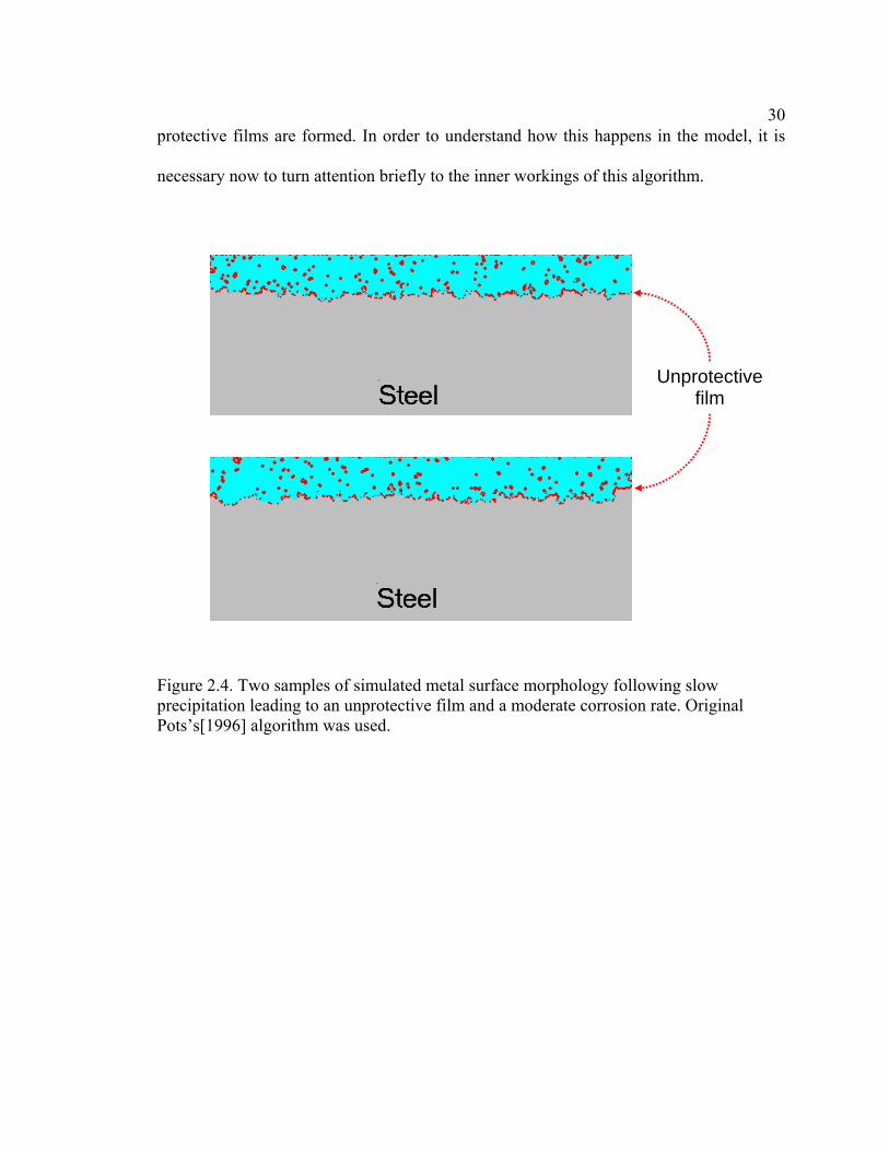
30protective films are formed. In order to understand how this happens in the model, it is

necessary now to turn attention briefly to the inner workings of this algorithm.

Unprotective film

Figure 2.4. Two samples of simulated metal surface morphology following slow precipitation leading to an unprotective film and a moderate corrosion rate. Original Pots’s[1996] algorithm was used.

31

Partially protective

film

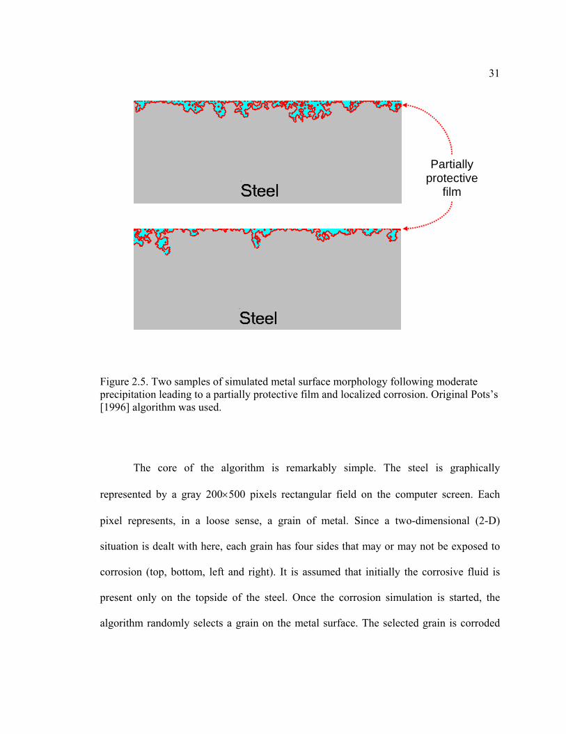
Figure 2.5. Two samples of simulated metal surface morphology following moderate precipitation leading to a partially protective film and localized corrosion. Original Pots’s [1996] algorithm was used.

The core of the algorithm is remarkably simple. The steel is graphically

represented by a gray 200×500 pixels rectangular field on the computer screen. Each

pixel represents, in a loose sense, a grain of metal. Since a two-dimensional (2-D)

situation is dealt with here, each grain has four sides that may or may not be exposed to

corrosion (top, bottom, left and right). It is assumed that initially the corrosive fluid is

present only on the topside of the steel. Once the corrosion simulation is started, the

algorithm randomly selects a grain on the metal surface. The selected grain is corroded

32by decreasing its associated corrosion index (CI) by an amount, which is linearly

proportional to the number of sides, Θ, the grain has exposed to the solution. The rule is:

Θ−= 4oldnew CICI (2-13)

According to this rule, the grain which has three sides exposed corrodes (its CI

has been reduced) three time faster than the grain with only one side exposed. Initially,

all the grains on the top layer have only one side exposed (Θ=1) and all the other internal

grains have no exposed sides (Θ=0). This changes as the simulation progresses and the

grains get corroded away. If it happens that all the grains around a particular grain

corrode away, that grain with Θ=4 will become detached and will be removed from the

remaining simulation process. Every grain starts out with the same, arbitrarily chosen,

corrosion index, CI=10, and is corroded away when CI decreases to or below zero. When

this happens, the corresponding steel pixel is removed from the simulation.

Correspondingly, it changes its color from gray to blue on the computer screen.

During the simulation, precipitation of a film happens along with corrosion in

alternating steps. The algorithm performs the precipitation step by randomly selecting a

grain where precipitation will happen. Precipitation is simulated by increasing a film

index, FI, for that particular grain. Every grain starts out without any film, FI=0. If it is

hit by precipitation, its film index is increased until FI≥10 at which point that this

particular grain has a very dense film and is fully protected from corrosion. On the screen,

this is demonstrated by a pixel turning red above the protected pixel. Every time the

precipitation process randomly “hits” a grain. Then its film index increases by an amount

33which is proportional to the number of sides, Θ, under the condition that particular grain

has exposed to the solution and the scaling tendency, ST. The rule is:

STFIFI oldnew Θ+= 8 (2-14)

Obviously when there is no precipitation (ST=0), the film index FI will not

change during the simulation. Vice versa, when the precipitation rate is high (ST≈1), the

film index for any particular grain will rapidly reach (in one or two hits) the maximum

value of 10, at which point the film is considered to be fully protective.

The simple algorithm described above works remarkably well and produces a

wide range of corrosion surface morphologies as already illustrated in Figure 2.-Figure 2..

Even if there is not much explicit physico-chemical content built into the algorithm (other

then ST), the appearance of the 2-D corroded surface, including the one with localized

attack, is rather similar to what is seen in Scanning Electron Microscope (SEM) images

of corroded steel samples. This leads us to a conclusion that in order to get localized

attack, it is sufficient to have a partially protective film and stochastic corrosion and

precipitation processes. On a microscopic level, both the corrosion and the precipitation

processes are stochastic in nature due to a constant interchange of cathodes and anodes,

inhomogeneous steel surface metallurgy, stochastic nature of the diffusion process, to

name just a few arguments. Therefore, it can be concluded that the only condition that is

needed to get localized attack is partially protective film, which is the same conclusion

that Sun and Nesic [2003] reached by analyzing long-term CO2 corrosion experiments in

wet gas flow. It can be argued that this is a “minimum requirement” for localized

34corrosion, notwithstanding the fact that other factors such as hydrodynamics, steel

composition, inclusions, etc. might complicate the situation further.

Pots’s model works remarkably well to provide all the various forms of corrosion

attack by varying a single parameter, the scaling tendency. Since scaling tendency is

related to nearly all the primitive parameters that affect localized corrosion, this thesis

will use Pots’s model as a starting point to build a more advanced localized corrosion

model.

35CHAPTER 3

MODEL DEVELOPMENT

Pots’s original algorithm requires only one input: the scaling tendency ST. This

apparent strength is its weakness as well, since knowing ST is not straightforward. ST

depends on the precipitation rate as well as the corrosion rate as shown by equation (2-

12). Neither of the two is easy to be predicted as they depend on many factors including

water chemistry, steel composition, surface electrochemistry, transport of species in the

solution, etc. Therefore, given that one knows the primitive input parameters such as

temperature, pH, velocity, etc., a model is needed to predict the corrosion and

precipitation rates, before ST can be found.

The second weakness of the original algorithm lies in the arbitrariness of the

constants used in the rules expressed in the former chapter. The constants in equations (2-

13) and (2-14) have been adjusted relative to each other to give plausible answers in

terms of morphology of the corrosion attack. However, the answer is qualitative and one

cannot deduce the magnitude of the attack, be it uniform or local.

All of the above weaknesses can be overcome and the detailed method will be

explained in the following paragraphs. The rules of the original algorithm were also

scrutinized and modified to make the simulation perform more reasonably.

Before any modification was carried out, the number of repetitions of the two

processes (corrosion and precipitation) for each simulation has been increased 20 times.

The maximum depth vs. time curve has been substituted by the maximum penetration

36rate vs. time curve because the latter makes more practical sense. Uniform corrosion rate

vs. time curve has been calculated and drawn on the same graph.

3.1 Modification of the Corrosion Rule

In the original algorithm, the rate of corrosion of any particular grain on the steel

surface is proportional to its exposed surface area. In terms of the rules defined above, the

decrease of the corrosion index CI is only proportional to the number of sides - Θ, which

that particular grain has exposed to the solution (see equation 2-13). However, the

corrosion rate of any particular grain should also be related to the presence of a protective

film. The algorithm described above takes this into account only in a binary sense, i.e.,

when the film index, FI, increases to or above 10, the grain is considered fully protected

and cannot be corroded further. What the original algorithm does not take into account is

the effect of partially protective film. It is known that surface films range in

protectiveness from unprotective to mildly and to very protective depending on their

density/porosity. This can easily be accommodated by the rules above as the film index,

FI, which varies from 0 to 10, can be seen as an indicator of film protectiveness. We can

assume that the higher the FI is for a particular grain, the slower it will corrode.

Therefore, equation (2-13) can be modified as follows:

1010

14 <⎟⎠⎞

⎜⎝⎛ −Θ−= FIFICICI oldnew (3-1)

10≥= FICICI oldnew (3-2)

37When there is no film, i.e., for the grain FI=0, the equation works in the same way

as equation (2-13). However, the change in the grain CI, i.e., its corrosion rate, slows

down as the grain FI increases due to buildup of a protective film. Eventually, when the

film becomes fully protective (the grain FI=10), corrosion is hindered and equation (3-1)

predicts that the grain CI stops decreasing. In other words, the modification makes the

new algorithm work like the original one at the extremes (no-film and fully protective

film situations). What is more important, it adds the intermediate effect of partially

protective films.

3.2 Modification of Precipitation Rule

To initiate precipitation, the solution must be supersaturated. The precipitation

takes place in two stages: nucleation and growth of these nuclei to macroscopic scale

[Calarch 2001]. It is not easy to detect formation of sub-micronic nuclei and generally

both nucleation and growth occur simultaneously in solution. It is well known that the

addition of small “seed” particles to a supersaturated solution can greatly increase the rate

at which crystals nucleate. The classical theory of nucleation provides a natural

explanation as to why a seed crystal facilitates crystal nucleation: in order to grow,

crystallites of the stable phase need to exceed a critical size. Crystallites that are smaller

than this “critical nucleus” dissolve again while larger crystallites can grow to a

macroscopic size. In the absence of a seed, a rare, spontaneous fluctuation is needed to

form a crystal nucleus that exceeds the critical size [Cacciuto 2004].

Nucleation theory is based upon thermodynamic models which link nucleation

rate to supersaturation [Calarch 2001]. According to Johnson [Johnson 1991], scale

38

ttSTFIFI >Θ+= 4

nucleation may be related to precipitation rate. At a high precipitation rate, iron carbonate

may rapidly nucleate and grow to form a thin tight surface film. At a low precipitate rate,

precipitation may proceed so slowly (due to loss of nucleation center) that the crystals

either are swept away or grow in irregular islands on the surface.

Nucleation process, which has not been considered in Pots’ original algorithm, is

implemented in this thesis’s model by performing the following precipitation rules:

critoldnew (3-3)

critAcrit

oldnew ttttSTFIFI <<Θ+= 04

A

STΘ

(3-4)

where A is a constant greater than one. The value of A and its physical meaning are

demonstrated below. Here it is assumed that there exists a time period that both

nucleation and crystal growth account for the increase of film index. The reason is that it

takes time for iron carbonate to aggregate, to form crystals that exceed a critical size, and

then to precipitate. Beyond that time period, this barrier disappears when a large amount

of crystallites form. Then only crystal growth, which can be represented by precipitation

rate, could influence the increase of film index. This period of time is defined as the time

interval from the beginning to a critical time, which is controlled by super saturation

[Calarch 2001]. From equation (2-10), it is known that super saturation is related to RPR,

and RPR is proportional to ST. So tcrit is related to ST. Higher ST results in smaller tcirt. So

tcrit is reversely proportional to ST. During the period of time between t=0 and t=tcrit, it is

assumed that the precipitation rate is increased from 0 (when t =0) to its full developed

rate 4 (when t = tcrit) with a quadratic function with respect to time. That means A

39=2, which is determined by comparing to experimental data. The chosen value of A

demonstrates that the precipitation is harder at the beginning of process when there are no

or little nuclei in the system. With the increase of the amount of nuclei, precipitation

becomes easier.

Note that the constant that determines how fast the film will precipitate has been

decreased from 8 in equation (2-14) to 4 in equation (3-3) and (3-4) to balance the

decrease of corrosion rate which resulted due to the modified rules.

The effect of the modified rules on localized attack is illustrated in Figure 3.1. A

larger variety of surface morphologies are now obtained over a broader range of ST. Pits

are narrow toward the bottom as well as “mushroom” style pits appear at various ST. In

certain cases, pits propagate much deeper and even fail to heal.

Various steel surface morphologies obtained in the simulations are compared with

selected SEM images taken from a CO2 corrosion study in multiphase flow by Nesic and

Lunde [1994] (see Figure 3.2.). It clearly confirms that the algorithm proposed above is

capable of predicting qualitatively a wide range of localized attack morphologies seen in

practice.

40

ST =0.53 ST =0.45

ST =0.57ST =0.72

Figure 3.1. Surface morphology prediction taken from the study of 2-D localized corrosion model by Nesic, Xiao, and Pots [2004]

Figure 3.2. SEM images of the corroded steel surfaces taken from the study of CO2 corrosion in multiphase flow taken from the study by Nesic and Lunde [1994].

413.3 Link to OU 1-D Mechanistic Model

As mentioned at the beginning of this chapter, there are two obvious weaknesses

in Pots’s original algorithm. One is that the model only depends on ST and another is that

its value is not easier to be obtained. Both weaknesses can be eliminated by linking the

algorithm with a corrosion/precipitation model that can predict the scaling tendency ST

and uniform corrosion rate. Hence, the morphology and the magnitude of the attack can

be predicted. For this purpose, the mechanistic one-dimensional (1-D) CO2 corrosion

model of Nesic [2003] has been used in this thesis.

For the purposes of connecting it with the 2-D algorithm described above, it is

required to compute the scaling tendency at the steel surface where the films form.

Therefore one needs information about the solution chemistry at the steel surface, which

can be very different from the one in the bulk, particularly if some sort of surface film is

already in place. Further, the scaling tendency changes with time as the corrosion and

precipitation rate change. Very few corrosion/precipitation models can satisfy this

requirement.

The recent 1-D mechanistic model of Nesic [Nordsveen 2003, Nesic and Lee

2003, Nesic 2003] is a perfect candidate for linkage with the 2-D algorithm described

above as it computes concentration profiles of all species involved in the

corrosion/precipitation reactions. The model covers most of the important processes

present in uniform CO2 corrosion of carbon steel:

• Electrochemical reactions at the steel surface,

42• Chemical reactions including precipitation and

• Transport of species between the steel surface and the bulk solution including

transport through the porous corrosion film.

The physical, mathematical and numerical aspects of the proposed model are

explained in detail in the original papers; however a very brief outline is given below to

facilitate the understanding of the text to follow. Since it is a model of uniform corrosion,

a one-dimensional computational domain is used, stretching from the steel surface

through the pores of a surface film and the mass transfer boundary layer, ending in the

turbulent bulk of the solution. Detail description of this model can be found in Nesic et al.

[Nesic and Lee 2003, Nesic and Nordsveen 2003, Nesic 1996] paper.

The concentration of each species is governed by a species conservation (mass

balance) equation. A universal form of the equation which describes transport for species

j in the presence of chemical reactions, which is valid both for the liquid boundary layer

and the porous film, is:

( ){

reactions chemical toduesinkor source

fluxnet

5.1

onaccumulati

jjeff

jj R

xc

Dxt

cε

∂∂

ε∂∂

∂ε∂

+⎟⎟⎠

⎞⎜⎜⎝

⎛=

444 3444 21321

(3-5)

where cj is the concentration of species j in kmol m-3, ε is the porosity of the film, Djeff

is

the effective diffusion coefficient of species j (which includes both the molecular and the

turbulent component) in m2 s-1, Rj is the source or sink of species j due to all the chemical

reactions in which the particular species is involved in kmol m-3s-1, t is time and x is the

43spatial coordinate in m. It should be noted that in the transport equation above

electromigration has been neglected as its contribution to the overall flux of species is

small. Turbulent convection has been replaced by turbulent diffusion as the former is

difficult to determine explicitly in turbulent flow.

One equation of the form (3-5) is written for each species. They all are solved

simultaneously in space and time. The boundary conditions for this set of partial

differential equations are: in the bulk - equilibrium concentrations of species (which is

also used as the initial condition), and at the steel surface - a flux of species is determined

from the rate of the electrochemical reactions (zero flux for non-electroactive species).

Once the set of equations is solved in any given time step, the uniform corrosion rate, CR,

can be simply calculated as the flux of Fe2+ ions at the metal surface.

Solid iron carbonate (FeCO3), which is treated as one of the species, will

precipitate when the iron carbonate saturation exceeded according to (2-5).

From the two different expressions describing the kinetics of iron carbonate

precipitation proposed by Johnson [1991] and Van Hunnik [1996], the latter (equation 2-

10) is used because it is believed to give more realistic results especially at higher super

saturation.

Once the rate of precipitation, R , and the uniform corrosion rate, CR, are

calculated as a function of the input parameters such as temperature, pH, partial pressure

of CO

)(3 sFeCO

2, velocity, etc., the scaling tendency ST can be computed according to equation (2-

12) and used as an input into the 2-D model.

44Table 1 lists the test conditions used to calibrate the 1-D mechanistic model and

2-D localized corrosion model. Since different ST give different morphologies of surface,

table 1 lists conditions that will give a variety of ST. Some film forming conditions are

also listed to calibrate the precipitation rate and hence to obtain the maximum penetration

rate.

Table 1. Test Matrix

Parameters Conditions CO2 partial pressure (bar) 2, 1, 0.54 Solution 1% NaCl, distillation waterpH 5.8, 6.0, 6.3, 6.5, 6.6 single-phase flow (m/s) 1, 0.2 Temperature (ºC) 50, 55, 65, 80 Test time (hrs) 50 Iron concentration (ppm) 5, 25, 50, 100

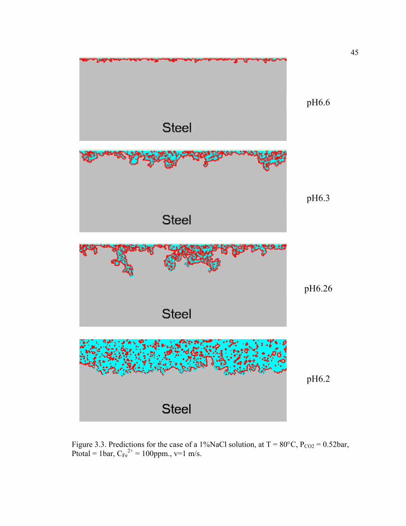
An illustration of the integrated 2-D model at work is shown in Figure 3.3. Under

those conditions one gets a very protective film at pH6.6, only a partially protective film

and some initial localized attack (which heals) at pH6.3, poorly protective film and

progressive localized attack at pH6.26 and unprotective films and uniform attack at

pH6.2 and lower.

45

pH6.6

pH6.3

pH6.26

pH6.2

Figure 3.3. Predictions for the case of a 1%NaCl solution, at T = 80°C, PCO2 = 0.52bar, Ptotal = 1bar, CFe

2+ = 100ppm., v=1 m/s.

463.4 Film Growth Algorithm

Film precipitation is one of the two crucial processes in this simulation, and the

rules it performs have been fully described in equations (3-3) and (3-4). But the growth of

the film has not been considered in the previous work, and neither has its effect on

corrosion. As we know, in reality, as long as the solution is supersaturated, iron carbonate

will continuously precipitate and layers upon layers of films form. Thus, a film growth

algorithm needs to be implemented to make the whole simulation perform more

realistically.

The film grows according to the precipitation rate. As mentioned above, when a

grain is hit by a random film process, its FI will be increased based on equation (3-3) or

(3-4). If the film index is above 10, film forms. In the previous work, the simulation did

not perform differently when the film index was greater then 10, because film growth

was not built in. However, film index is a good indicator to be used for predicting the

thickness of the film.

The film can protect not only the steel grain it covers on top but also to some

extent its neighbors. As each grain has four neighbors, there are four possible exposed

sides. A film that precipitates on any of the four neighbors hinders the corrosion of that

specific grain from that side, and the possibility for that specific grain to corrode

decreases as the number of exposed sides decrease. The influence of this effect is more

obvious when the film grows quickly.

47

)1*( STL −

The film is more stable when the ST is high because higher ST usually results in

protective film. When the precipitation rate is high compared to uniform corrosion rate,

the film is denser and the distance between the film and bare metal is shorter, which

means the film is more resistant to being swept away by the flow [Johnson 1991]. On the

contrary, when the precipitation rate is low compared to corrosion rate, the formed film is

more porous and the distance between the film and bare metal could be quite large and

hence, could easily be removed by the flow. So, the ability for the next layer of film to

grow varies with surface scaling tendency. Even at the same surface scaling tendency,

the film grows easier when it is close to metal surface due to less turbulence reaching the

surface through the boundary layer. This is modeled by the following equation i.e. when

a

*10*)1( ALFI +> (3-6)

then a new film layer forms. Here L represents the number of layers of film for a specific

steel grain. A is a constant greater than 1. This formula clearly shows that the higher the

scaling tendency is, the easier it is for the next layer of film to form; the smaller the L is,

the easier it is for the next layer of film to form. The values of A and L need to be

calibrated with experimental data.

The algorithm of iron carbonate film growth was implemented in an easy way at

first. It was considered the film deposited directly on top of the previous film. Figure 3.4

shows typical film morphology obtained in simulation studies. From this figure, a clear

solution layer, a porous film layer, a dense film layer, and the detached layer between

film and metal can be easily observed from top to bottom. Comparison with the various

48

film morphologies on the selected SEM image (see Figure 3.5) taken from a CO2

corrosion precipitation study by Lee [2003], confirms the existence of all the above layers.

Figure 3.4 Film morphology taken from the proposed 2-D Model.

steel

iron carbonate film 4-6 µm

epoxydenselayer

porouslayer

Figure 3.5 SEM image of a cross section of a steel specimen including an iron carbonate film. Exposed for 10 hours at T=80°C, pH 6.6, = 0.54 bar, = 250 ppm, v=1 m/s.

2COP +2Fec

49

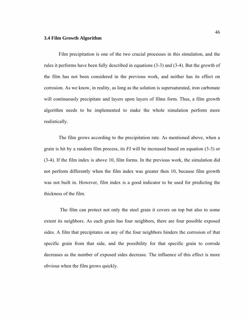
Figure 3.6 Comparison of the film morphology before (top) and after (bottom) using a random film formation algorithm at pH 6.6, 80oC, 5ppm Fe2+ and 0.52bar pCO2.

The computer screen displays only part of the film, which grows in the domain of

the original piece of metal. Actually, the film could grow far beyond the location of the

original piece of metal out to the bulk. But in order to create a tidy display, we chose not

to show it.

From Figure 3.4, it is seen that the structure of the film does not seem realistic. In

reality, the film deposits randomly in any direction instead of only vertically. And the

structure of crystallites is more porous with self similarity properties like fractals [Joosten

1992]. Fractals are objects with self-similar structures on different scales. In the present

model, a random process has been implemented to allow the next layer of film to choose

the direction it deposits. The direction could be left, right and top, and the newly formed

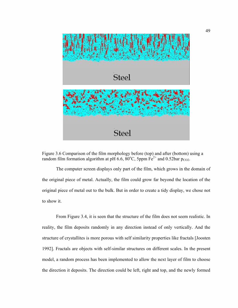
50film structure is more porous than the previous one. Figure 3.6 and 3.7 show the

comparison of the film structures.

The new film structure expands more horizontally than vertically and this

property affects the coverage of the surface around the center of the film deposition.

From figure 3.8, we see that the shape of the pit becomes more bowl-like with this

modification, while it is sharper in the previous version of the model.

Figure 3.7 Comparison of the film morphology at higher magnification before (top) and after (bottom) using a random film formation algorithm at pH 6.6, 80oC, 5ppm Fe2+ and 0.52bar pCO2.

51

Figure 3.8 Comparison of the film morphology before (top) and after (bottom) using a random film formation algorithm at pH 6.5, 80oC, 50ppm Fe2+ and 0.52bar pCO2.

3.5 Implementation a Path-Searching Algorithm to Remove Isolated Islands

During a uniform corrosion process, the anodic and cathodic anodes switch back

and forth so that the metals at different locations corrode with the same rate. When an

iron carbonate film forms, the surface condition is not the same any more because of the

protective property of the iron carbonate film. Part of the surface base could still be

exposed, leaving the other parts protected. As the protected part of the surface becomes

passivated and becomes a cathode, the exposed surface as the anode corrodes more

quickly due to large surface ratio of cathode to anode (Sc/Sa). Subsequently, a rough

52surface forms and some metal could be detached from the base due to the corrosion

occurring beneath them (undercutting).

This phenomenon has been observed experimentally. According to Jaycock

[1998], pitting tends to undercut the surface, forming lacy covers (lace like structure) that

help them to maintain a concentrated local chemistry. At the edges of the pit, transport of

metal ions into bulk solution is relatively rapid and the local concentration falls below the

critical value, causing these areas to repassivate. Deeper into the pit cavity, active

dissolution continues such that pit growth undercuts the passivated material and

eventually breaks through the surface from beneath. Metal ions diffuse rapidly through

the new hole, again causing the local concentration to fall and repassivation to occur.

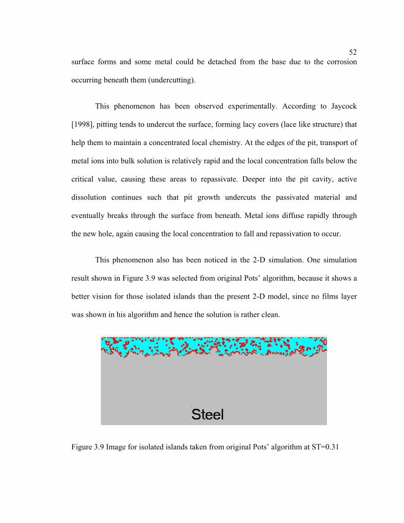
This phenomenon also has been noticed in the 2-D simulation. One simulation

result shown in Figure 3.9 was selected from original Pots’ algorithm, because it shows a

better vision for those isolated islands than the present 2-D model, since no films layer

was shown in his algorithm and hence the solution is rather clean.

Figure 3.9 Image for isolated islands taken from original Pots’ algorithm at ST=0.31

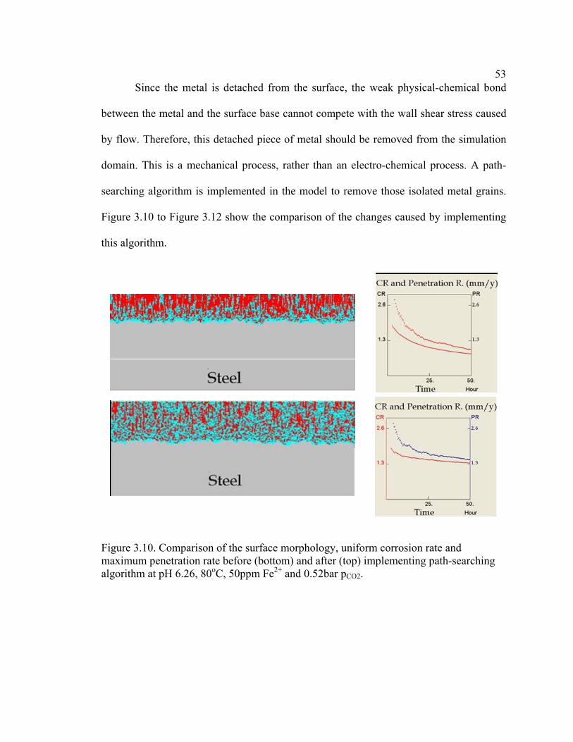
53Since the metal is detached from the surface, the weak physical-chemical bond

between the metal and the surface base cannot compete with the wall shear stress caused

by flow. Therefore, this detached piece of metal should be removed from the simulation

domain. This is a mechanical process, rather than an electro-chemical process. A path-

searching algorithm is implemented in the model to remove those isolated metal grains.

Figure 3.10 to Figure 3.12 show the comparison of the changes caused by implementing

this algorithm.

Figure 3.10. Comparison of the surface morphology, uniform corrosion rate and maximum penetration rate before (bottom) and after (top) implementing path-searching algorithm at pH 6.26, 80oC, 50ppm Fe2+ and 0.52bar pCO2.

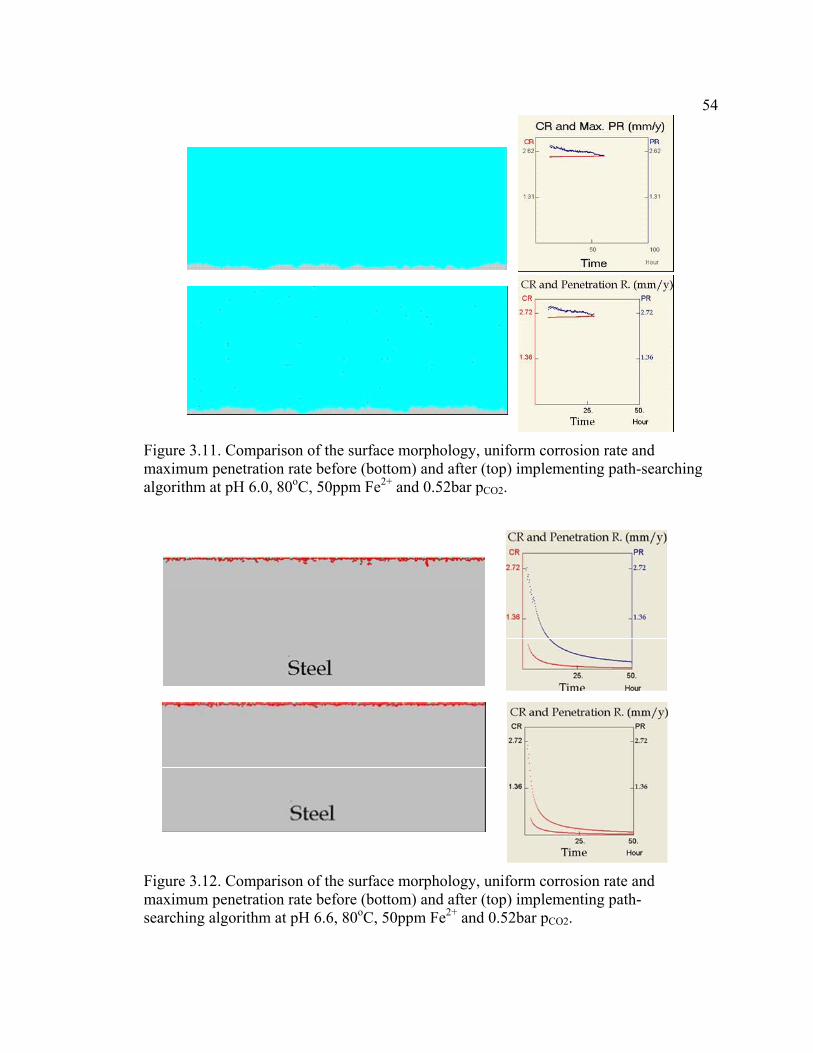
54



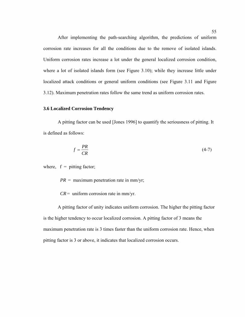
55After implementing the path-searching algorithm, the predictions of uniform

corrosion rate increases for all the conditions due to the remove of isolated islands.

Uniform corrosion rates increase a lot under the general localized corrosion condition,

where a lot of isolated islands form (see Figure 3.10); while they increase little under

localized attack conditions or general uniform conditions (see Figure 3.11 and Figure

3.12). Maximum penetration rates follow the same trend as uniform corrosion rates.

3.6 Localized Corrosion Tendency

A pitting factor can be used [Jones 1996] to quantify the seriousness of pitting. It

is defined as follows:

CRPRf = (4-7)

where, f = pitting factor;

PR = maximum penetration rate in mm/yr;

CR = uniform corrosion rate in mm/yr.

A pitting factor of unity indicates uniform corrosion. The higher the pitting factor

is the higher tendency to occur localized corrosion. A pitting factor of 3 means the

maximum penetration rate is 3 times faster than the uniform corrosion rate. Hence, when

pitting factor is 3 or above, it indicates that localized corrosion occurs.

56

CHAPTER 4

VERIFICATION

4.1 Comparisons

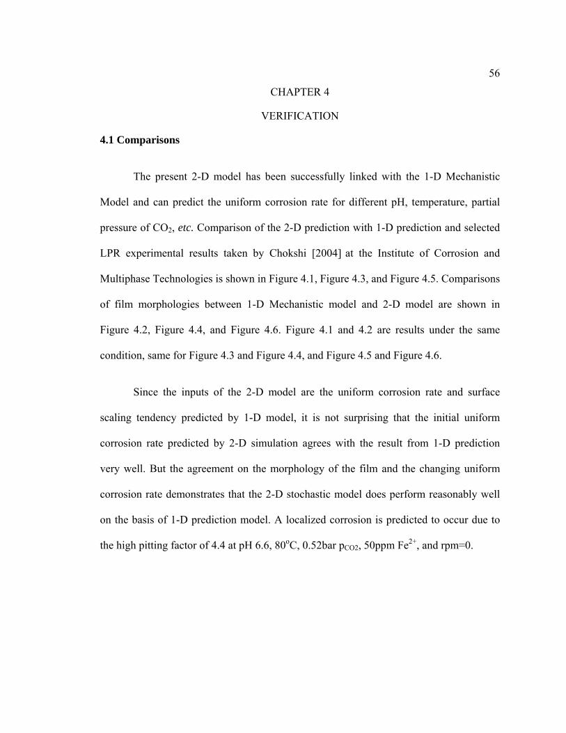
The present 2-D model has been successfully linked with the 1-D Mechanistic

Model and can predict the uniform corrosion rate for different pH, temperature, partial

pressure of CO2, etc. Comparison of the 2-D prediction with 1-D prediction and selected

LPR experimental results taken by Chokshi [2004] at the Institute of Corrosion and

Multiphase Technologies is shown in Figure 4.1, Figure 4.3, and Figure 4.5. Comparisons

of film morphologies between 1-D Mechanistic model and 2-D model are shown in

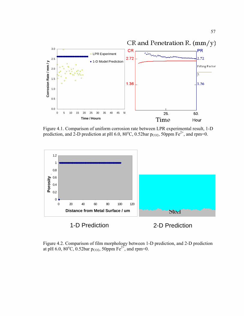
Figure 4.2, Figure 4.4, and Figure 4.6. Figure 4.1 and 4.2 are results under the same

condition, same for Figure 4.3 and Figure 4.4, and Figure 4.5 and Figure 4.6.

Since the inputs of the 2-D model are the uniform corrosion rate and surface

scaling tendency predicted by 1-D model, it is not surprising that the initial uniform

corrosion rate predicted by 2-D simulation agrees with the result from 1-D prediction

very well. But the agreement on the morphology of the film and the changing uniform

corrosion rate demonstrates that the 2-D stochastic model does perform reasonably well

on the basis of 1-D prediction model. A localized corrosion is predicted to occur due to

the high pitting factor of 4.4 at pH 6.6, 80oC, 0.52bar pCO2, 50ppm Fe2+, and rpm=0.

57

0.0

0.5

1.0

1.5

2.0

2.5

3.0

0 5 10 15 20 25 30 35 40 45 50

Time / Hours

Cor

rosi

on R

ate

/ mm

/ y

LPR Experiment

1-D Model Prediction

Figure 4.1. Comparison of uniform corrosion rate between LPR experimental result, 1-D prediction, and 2-D prediction at pH 6.0, 80oC, 0.52bar pCO2, 50ppm Fe2+, and rpm=0.

2-D Prediction1-D Prediction

0

0.2

0.4

0.6

0.8

1

1.2

0 20 40 60 80 100 120

Distance from Metal Surface / um

Poro

sity


Poro

sity

Figure 4.2. Comparison of film morphology between 1-D prediction, and 2-D prediction at pH 6.0, 80oC, 0.52bar pCO2, 50ppm Fe2+, and rpm=0.

58

0.0

0.5

1.0

1.5

2.0

2.5

3.0

0 5 10 15 20 25 30 35 40 45 50

Time / Hours

Cor

rosi

on R

ate

LPR Experiment

1-D Model Prediction

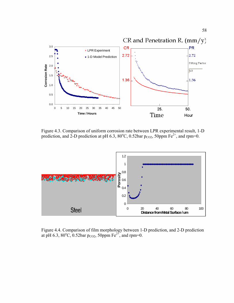
Figure 4.3. Comparison of uniform corrosion rate between LPR experimental result, 1-D prediction, and 2-D prediction at pH 6.3, 80oC, 0.52bar pCO2, 50ppm Fe2+, and rpm=0.

0

0.2

0.4

0.6

0.8

1

1.2

0 20 40 60 80 10Distance from Metal Surface / um

Poro

sity

0

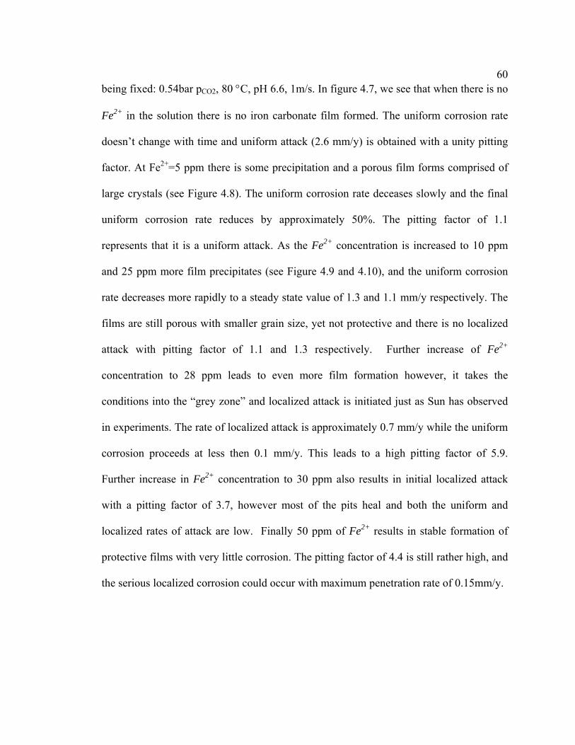
Figure 4.4. Comparison of film morphology between 1-D prediction, and 2-D prediction at pH 6.3, 80oC, 0.52bar pCO2, 50ppm Fe2+, and rpm=0.

59

0.00

0.50

1.00

1.50

2.00

2.50

3.00

0 5 10 15 20 25 30 35 40 45 50

Time / hr

CR

/ mm

/yr

LPROU Model

Figure 4.5. Comparison of uniform corrosion rate between LPR experimental result, 1-D prediction, and 2-D prediction at pH 6.6, 80oC, 0.52bar pCO2, 50ppm Fe2+, rpm=0.

0

0.2

0.4

0.6

0.8

1

1.2

0 5 10 15 20 25


Poro

sity

Figure 4.6. Comparison of film morphology between 1-D prediction, and 2-D prediction at pH 6.6, 80oC, 0.52bar pCO2, 50ppm Fe2+, rpm=0.

4.2 Parametric study

The surface morphologies and uniform corrosion rate vs. time curve predicted by

the 2-D model are shown in Figure 4.7, Figure 4.8, Figure 4.9, Figure 4.10, Figure 4.11,

Figure 4.12, and Figure 4.13 by varying ferrous iron concentration for all other conditions

60being fixed: 0.54bar pCO2, 80 °C, pH 6.6, 1m/s. In figure 4.7, we see that when there is no

Fe2+ in the solution there is no iron carbonate film formed. The uniform corrosion rate

doesn’t change with time and uniform attack (2.6 mm/y) is obtained with a unity pitting

factor. At Fe2+=5 ppm there is some precipitation and a porous film forms comprised of

large crystals (see Figure 4.8). The uniform corrosion rate deceases slowly and the final

uniform corrosion rate reduces by approximately 50%. The pitting factor of 1.1

represents that it is a uniform attack. As the Fe2+ concentration is increased to 10 ppm

and 25 ppm more film precipitates (see Figure 4.9 and 4.10), and the uniform corrosion

rate decreases more rapidly to a steady state value of 1.3 and 1.1 mm/y respectively. The

films are still porous with smaller grain size, yet not protective and there is no localized

attack with pitting factor of 1.1 and 1.3 respectively. Further increase of Fe2+

concentration to 28 ppm leads to even more film formation however, it takes the

conditions into the “grey zone” and localized attack is initiated just as Sun has observed

in experiments. The rate of localized attack is approximately 0.7 mm/y while the uniform

corrosion proceeds at less then 0.1 mm/y. This leads to a high pitting factor of 5.9.

Further increase in Fe2+ concentration to 30 ppm also results in initial localized attack

with a pitting factor of 3.7, however most of the pits heal and both the uniform and

localized rates of attack are low. Finally 50 ppm of Fe2+ results in stable formation of

protective films with very little corrosion. The pitting factor of 4.4 is still rather high, and

the serious localized corrosion could occur with maximum penetration rate of 0.15mm/y.

61

Figure 4.7 Film morphology and corresponding corrosion rate predicted by 2-D model at 0.54bar pCO2, 0ppm Fe2+, 80 °C, pH 6.6, 1m/s

Figure 4.8 Film morphology and corresponding corrosion rate predicted by 2-D model at 0.54bar p , 5ppm Fe , 80 °C, pH 6.6, 1m/s CO2

2+


62



63



64CHAPTER 5

CONCLUSIONS

The original two-dimensional (2-D) stochastic algorithm by van Hunnik and Pots

[1996] was modified to enable a simulation of localized corrosion morphologies found in

practice. The added film formation algorithm and nucleation algorithm predict more

realistic film morphology and uniform corrosion rate. The added path searching

algorithm improves the quality of prediction.

The original Pots [1996] algorithm, which uses scaling tendency as the only input

parameter, was connected with the mechanistic model of Nešić{2003], so that localized

attack could be predicted as a function of primitive parameters such as temperature, pH,

partial pressure of CO2, velocity.

The 2-D model has been successfully calibrated at different film precipitation

conditions. Based on the results of the simulations, it was postulated that partially

protective films are all that is needed to trigger a localized attack, which is in agreement

with the experimental study of Sun [2003].

65CHAPTER 6

FUTURE WORK

The 2-D model has been carefully calibrated at low pressure (up to 2bar), high

temperature (up to 80°C) and various pH values. More experimental data (especially at

high pressure) needs to be obtained, so that the likelihood and magnitude of localized

attack can be precisely calibrated.

The mechanism behind the model may allow for it to be used in any

corrosion/coverage competition condition. Since we know that inhibitor carries out

coverage effect to protect the surface from corrosion, and same effect is performed by

H2S mackinawite. Extending the model under those conditions will extremely improve

the utility of the model.

It is suggested to extend the mechanistic 1-D transport/electrochemical model

completely into a 2-D model so that localized corrosion can be predicted by using a

surface scaling tendency varying with time and depth of the cavity. However, due to the

mathematical complexity, the merging of the two models in the presence of passive film

is not a simple task.

66REFERENCES

1. Bertocci U., Koike M., S. Leigh, Qiu F., and Yang G., J. Electrochem. Soc., 1986,

133, 1782.

2. Bertocci U., and Huet F., Corrosion, 1995, 51, 131.

3. Bowman C.W., “New Developments in the Use of Chemicals for Pipeline Corrosion

Control,” Corrosion Science in the 21st Century, UMIST, 2003.

4. Brossia C.S., and Cragnolino G.A., “Effect of Environmental Variables on Localized

Corrosion of Carbon Steel,” Corrosion, 2000, 56, 5.

5. Bursten, G. T., Pistorius, P.C., and Mattin, S.P., Corrosion Sci., 35, 57 (1993).

6. Cacciuto A, Auer S., and Frenkel D, “Onset of heterogeneous crystal nucleation in

colloidal suspensions”, Nature 428, 404 – 406, 2004.

7. Calarch Ph., “Theoretical Introduction to Precipitation's Phenomena”, published

online: 7 Mar 2001, at http://www.nano-tek.org/main.html.

8. Chen J.F., and Bogaerts W.F., “Electrochemical Emission Spectroscopy for

Monitoring Uniform and Localized Corrosion,” Corrosion, Vol. 52, No. 10, 1996, p.

753.

9. Chokshi K., Board Meeting Report, Sep, 2003.

10. Dabosi F., Beranger G., and Baroux B., Corrosion Localisee, les editions de

physique, France, 1994, p. 654.

http://www.nano-tek.org/main.html

6711. de Moraes, F., Shadley, J.R., Chen, J., “Characterization of CO2 Corrosion Product

Scales Related to Environmental Conditons,” Corrosion/2000, Paper No.30.

12. de Waard C., Lotz U., and Dugstad A., “Influence of Liquid Flow Velocity on CO2

Corrosion: A Semi-empirical Model,” CORROSION/95, Paper No. 254 (Houston,

TX: NACE International, 1995).

13. de Waard, C., Lotz, U., “Prediction of CO2 Corrosion of Carbon Steel,”

Corrosion/93, paper no. 69, (NACE international, Houston, TX: 1993).

14. de Waard, C., and Milliams, D.E., “ Carbonic Acid Corrosion of Steel,” Corrosion,

31, No.5, P.197, 1975.

15. Dugstad, A, Lunde, L., and Videm, K., “Parametric Study of CO2 Corrosion of

Carbon Steel,” Corrosion/94, Paper No.14.

16. Dugstad, A., “ The Importance of FeCO3 Supersaturation on the CO2 Corrosion of

Carbon Steels,” Corrosion/92, Paper No.14.

17. Fu S., Griffin A.M., Garcia J. G., and Young B., “A New Localized Corrosion

Monitoring Technique for the Evaluation of Oilfield Inhibitors,” CORROSION/1996,

Paper No. 346, NACE International, Houston, Texas, 1996.

18. Gabrielli C., Huet F., Keddam M., and Oltra R., Corrosion, 1990, 46, 266.

19. Gabrielli C., and Keddam, “Review of Applications of Impedance and Noise

Analysis to Uniform and Localized Corrosion,” M., Corrosion, 1992, 48, 794.

6820. Germerdonk K., “Inspection Data Manageet Challenge and Basis of Efficient Risk

Management,” CORROSION/99, Paper No. 535. (Houston, TX: NACE

International, 1999).

21. Gunaltun, Y.M. “Combining Research and Field Data for Corrosion Rate

Prediction,” CORROSION/96, Paper No. (Houston, TX: NACE International,

1996).

22. Hashimoto M., Miyajima S., and Murata T., Corrosion Science, 1992, 33, 885.

23. Heuer, J.K., Stubbins, J.F., “Microstructure Analysis of Coupons Exposed to Carbon

Dioxide Corrosion in Multiphase Flow”. Corrosion, 54, No.7, p.566, NACE, 1998.

24. Hoerle S., Sourisseau T., and Baroux B., “Effect of the Electrolyte Composition on

the Random/Deterministic Behaviours in Pitting Corrosion,” Electrochem. Society

Proceedings, Vol. 98, 17, 437.

25. http://www.corrosion-doctors.org/Localized/Introduction.htm.

26. Jaycock, N.J., and White, S.P., “A Model for Pit Propagation in Stainless Steels”,

Electrochemical Society Proceedings, Vol. 98-17, 469.

27. Johnson M. L., and Tomson M. B., “Ferrous Carbonate Precipitation Kinetics and

its Impact CO2 Corrosion,” Corrosion/1991, Paper No. 268, NACE International,

Houston, Texas, 1991.

28. Jones, D.A, Principles and Prevention of Corrosion, 2nd edition, Englewood Cliffs,

NJ : Prentice Hall ; London : Prentice-Hall International, 1996.

http://www.corrosion-doctors.org/Localized/Introduction.htm

6929. Joosten M.W., Johnsen T., Dugstad A., “In Situ Observation of Localized CO2

Corrosion,” CORROSION/94, Paper No. 3.

30. Joosten M.W., Johnsen T., Hardy H. H., Jossang T., and Feder J., “Fractal Behavior

of CO2 Pits”, Corrosion/92, Paper No. 11, NACE International, Houston, Texas,

1992.

31. Kaesche, H., “Corrosion of Metals: Physicochemical Principles and Current

Problems”, Springer, 2003, ISBN 3-540-00626-5.

32. Kermani, M.B., and Smith, L.M., “A Working Party Report on ‘CO2 Corrosion

Control in Oil and Gas Production’ Design Considerations”, European Federation of

Corrosion Publication, No.23, The Institute of Materials, 1997.

33. Marsh J., Palmer J.W., and Newman R.C., “Evaluation of Inhibitor Performance for

Protection against Localized Corrosion,” Corrosion/2002, Paper No. 2288, NACE

International, Houston, Texas, 2002.

34. Mullin, J.W., Crystallization, 3rd ed. Oxford, U.K.:Oxford Press, 1993.

35. Nesic S., Lee K. J., Corrosion, 2003, 59,616.

36. Nesic S., Nordsveen M., Nyborg R., and Stangeland A., “A Mechanistic Model for

Carbon Dioxide Corrosion of Mild Steel in the Presence of Protective Iron

Carbonate Films-Part 2: A Numerical Experiment”, Corrosion Science, 2003, 59,489.

37. Nesic S., and Lunde L., Corrosion, 1994, 50,717.

38. Nesic S., Postlethwaite J., and Olsen S., Corrosion, 1996, 52,280.

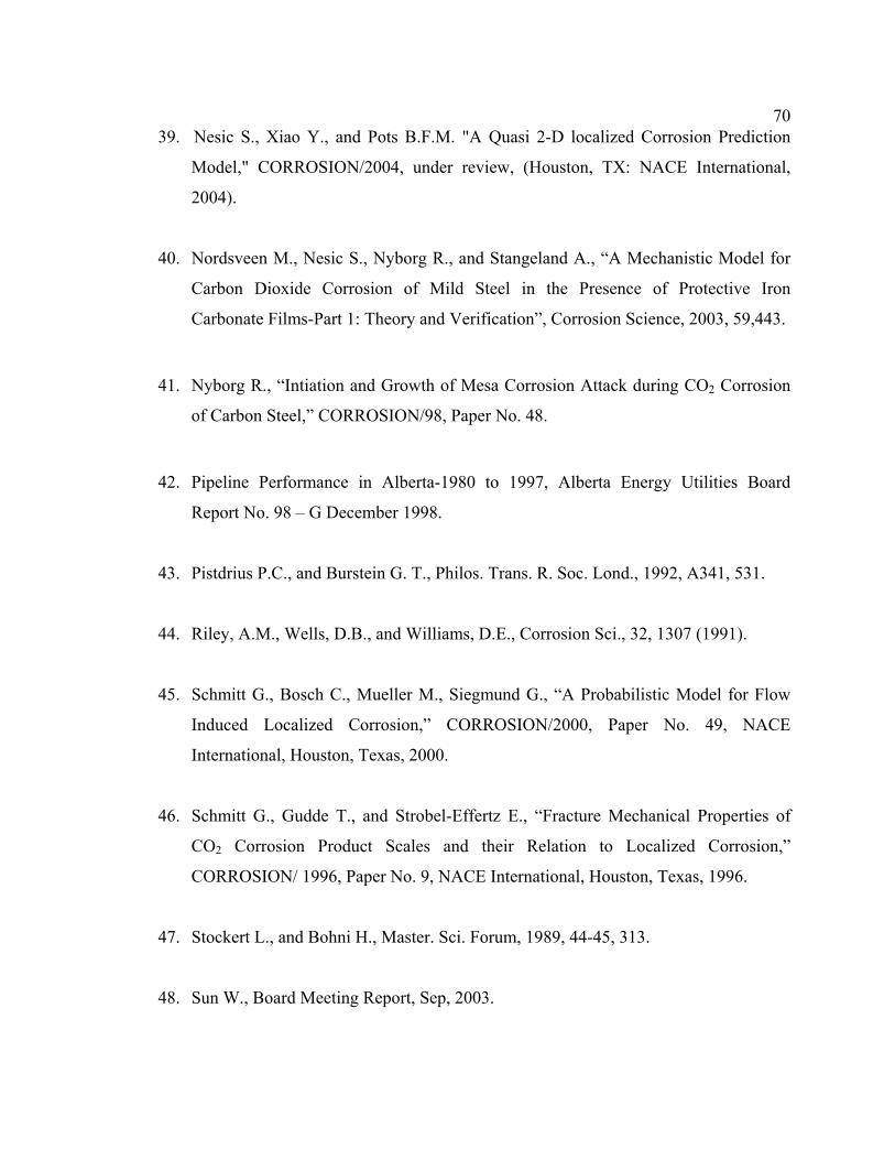
7039. Nesic S., Xiao Y., and Pots B.F.M. "A Quasi 2-D localized Corrosion Prediction

Model," CORROSION/2004, under review, (Houston, TX: NACE International,

2004).

40. Nordsveen M., Nesic S., Nyborg R., and Stangeland A., “A Mechanistic Model for

Carbon Dioxide Corrosion of Mild Steel in the Presence of Protective Iron

Carbonate Films-Part 1: Theory and Verification”, Corrosion Science, 2003, 59,443.

41. Nyborg R., “Intiation and Growth of Mesa Corrosion Attack during CO2 Corrosion

of Carbon Steel,” CORROSION/98, Paper No. 48.

42. Pipeline Performance in Alberta-1980 to 1997, Alberta Energy Utilities Board

Report No. 98 – G December 1998.

43. Pistdrius P.C., and Burstein G. T., Philos. Trans. R. Soc. Lond., 1992, A341, 531.

44. Riley, A.M., Wells, D.B., and Williams, D.E., Corrosion Sci., 32, 1307 (1991).

45. Schmitt G., Bosch C., Mueller M., Siegmund G., “A Probabilistic Model for Flow

Induced Localized Corrosion,” CORROSION/2000, Paper No. 49, NACE


46. Schmitt G., Gudde T., and Strobel-Effertz E., “Fracture Mechanical Properties of

CO2 Corrosion Product Scales and their Relation to Localized Corrosion,”

CORROSION/ 1996, Paper No. 9, NACE International, Houston, Texas, 1996.

47. Stockert L., and Bohni H., Master. Sci. Forum, 1989, 44-45, 313.

48. Sun W., Board Meeting Report, Sep, 2003.

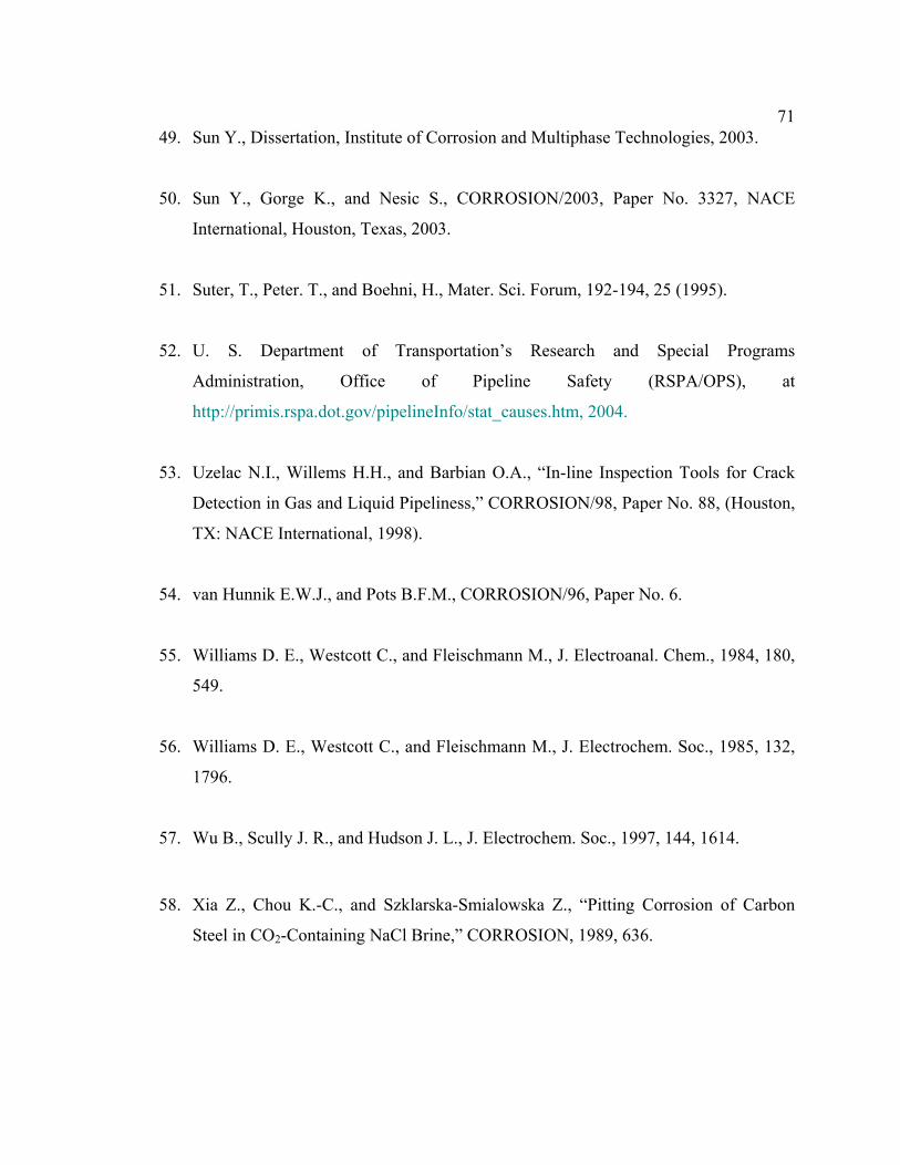
7149. Sun Y., Dissertation, Institute of Corrosion and Multiphase Technologies, 2003.

50. Sun Y., Gorge K., and Nesic S., CORROSION/2003, Paper No. 3327, NACE


51. Suter, T., Peter. T., and Boehni, H., Mater. Sci. Forum, 192-194, 25 (1995).

52. U. S. Department of Transportation’s Research and Special Programs

Administration, Office of Pipeline Safety (RSPA/OPS), at

http://primis.rspa.dot.gov/pipelineInfo/stat_causes.htm, 2004.

53. Uzelac N.I., Willems H.H., and Barbian O.A., “In-line Inspection Tools for Crack

Detection in Gas and Liquid Pipeliness,” CORROSION/98, Paper No. 88, (Houston,

TX: NACE International, 1998).

54. van Hunnik E.W.J., and Pots B.F.M., CORROSION/96, Paper No. 6.

55. Williams D. E., Westcott C., and Fleischmann M., J. Electroanal. Chem., 1984, 180,

549.

56. Williams D. E., Westcott C., and Fleischmann M., J. Electrochem. Soc., 1985, 132,

1796.

57. Wu B., Scully J. R., and Hudson J. L., J. Electrochem. Soc., 1997, 144, 1614.

58. Xia Z., Chou K.-C., and Szklarska-Smialowska Z., “Pitting Corrosion of Carbon

Steel in CO2-Containing NaCl Brine,” CORROSION, 1989, 636.

http://primis.rspa.dot.gov/pipelineInfo/stat_causes.htm, 2004

A TWO-DIMENSIONAL STOCHASTIC MODEL FOR … Two-Dimensional Stochastic... · 2.3 Film Formation and...

Documents

Transcript of A TWO-DIMENSIONAL STOCHASTIC MODEL FOR … Two-Dimensional Stochastic... · 2.3 Film Formation and...