A tutorial on support vector regression -...
77
Statistics and Computing 14: 199–222, 2004 C 2004 Kluwer Academic Publishers. Manufactured in The Netherlands. A tutorial on support vector regression ∗ ALEX J. SMOLA and BERNHARD SCH ¨ OLKOPF RSISE, Australian National University, Canberra 0200, Australia [email protected] Max-Planck-Institut f¨ ur biologische Kybernetik, 72076 T¨ ubingen, Germany [email protected] Received July 2002 and accepted November 2003 In this tutorial we give an overview of the basic ideas underlying Support Vector (SV) machines for function estimation. Furthermore, we include a summary of currently used algorithms for training SV machines, covering both the quadratic (or convex) programming part and advanced methods for dealing with large datasets. Finally, we mention some modifications and extensions that have been applied to the standard SV algorithm, and discuss the aspect of regularization from a SV perspective. Keywords: machine learning, support vector machines, regression estimation 1. Introduction The purpose of this paper is twofold. It should serve as a self- contained introduction to Support Vector regression for readers new to this rapidly developing field of research. 1 On the other hand, it attempts to give an overview of recent developments in the field. To this end, we decided to organize the essay as follows. We start by giving a brief overview of the basic techniques in Sections 1, 2 and 3, plus a short summary with a number of figures and diagrams in Section 4. Section 5 reviews current algorithmic techniques used for actually implementing SV machines. This may be of most interest for practitioners. The following section covers more advanced topics such as extensions of the basic SV algorithm, connections between SV machines and regularization and briefly mentions methods for carrying out model selection. We conclude with a discussion of open questions and problems and current directions of SV research. Most of the results presented in this review paper already have been published elsewhere, but the comprehensive presentations and some details are new. 1.1. Historic background The SV algorithm is a nonlinear generalization of the Gener- alized Portrait algorithm developed in Russia in the sixties 2 ∗ An extended version of this paper is available as NeuroCOLT Technical Report TR-98-030. (Vapnik and Lerner 1963, Vapnik and Chervonenkis 1964). As such, it is firmly grounded in the framework of statistical learn- ing theory, or VC theory, which has been developed over the last three decades by Vapnik and Chervonenkis (1974) and Vapnik (1982, 1995). In a nutshell, VC theory characterizes properties of learning machines which enable them to generalize well to unseen data. In its present form, the SV machine was largely developed at AT&T Bell Laboratories by Vapnik and co-workers (Boser, Guyon and Vapnik 1992, Guyon, Boser and Vapnik 1993, Cortes and Vapnik, 1995, Sch¨ olkopf, Burges and Vapnik 1995, 1996, Vapnik, Golowich and Smola 1997). Due to this industrial con- text, SV research has up to date had a sound orientation towards real-world applications. Initial work focused on OCR (optical character recognition). Within a short period of time, SV clas- sifiers became competitive with the best available systems for both OCR and object recognition tasks (Sch¨ olkopf, Burges and Vapnik 1996, 1998a, Blanz et al. 1996, Sch¨ olkopf 1997). A comprehensive tutorial on SV classifiers has been published by Burges (1998). But also in regression and time series predic- tion applications, excellent performances were soon obtained (M¨ uller et al. 1997, Drucker et al. 1997, Stitson et al. 1999, Mattera and Haykin 1999). A snapshot of the state of the art in SV learning was recently taken at the annual Neural In- formation Processing Systems conference (Sch¨ olkopf, Burges, and Smola 1999a). SV learning has now evolved into an active area of research. Moreover, it is in the process of entering the standard methods toolbox of machine learning (Haykin 1998, Cherkassky and Mulier 1998, Hearst et al. 1998). Sch ¨ olkopf and 0960-3174 C 2004 Kluwer Academic Publishers
Transcript of A tutorial on support vector regression -...

Statistics and Computing 14: 199–222, 2004C© 2004 Kluwer Academic Publishers. Manufactured in The Netherlands.
A tutorial on support vector regression∗
ALEX J. SMOLA and BERNHARD SCHOLKOPF
RSISE, Australian National University, Canberra 0200, [email protected] fur biologische Kybernetik, 72076 Tubingen, [email protected]
Received July 2002 and accepted November 2003
In this tutorial we give an overview of the basic ideas underlying Support Vector (SV) machines forfunction estimation. Furthermore, we include a summary of currently used algorithms for trainingSV machines, covering both the quadratic (or convex) programming part and advanced methods fordealing with large datasets. Finally, we mention some modifications and extensions that have beenapplied to the standard SV algorithm, and discuss the aspect of regularization from a SV perspective.
Keywords: machine learning, support vector machines, regression estimation
1. Introduction
The purpose of this paper is twofold. It should serve as a self-contained introduction to Support Vector regression for readersnew to this rapidly developing field of research.1 On the otherhand, it attempts to give an overview of recent developments inthe field.
To this end, we decided to organize the essay as follows.We start by giving a brief overview of the basic techniques inSections 1, 2 and 3, plus a short summary with a number offigures and diagrams in Section 4. Section 5 reviews currentalgorithmic techniques used for actually implementing SVmachines. This may be of most interest for practitioners.The following section covers more advanced topics such asextensions of the basic SV algorithm, connections between SVmachines and regularization and briefly mentions methods forcarrying out model selection. We conclude with a discussionof open questions and problems and current directions of SVresearch. Most of the results presented in this review paperalready have been published elsewhere, but the comprehensivepresentations and some details are new.
1.1. Historic background
The SV algorithm is a nonlinear generalization of the Gener-alized Portrait algorithm developed in Russia in the sixties2
∗An extended version of this paper is available as NeuroCOLT Technical ReportTR-98-030.
(Vapnik and Lerner 1963, Vapnik and Chervonenkis 1964). Assuch, it is firmly grounded in the framework of statistical learn-ing theory, or VC theory, which has been developed over the lastthree decades by Vapnik and Chervonenkis (1974) and Vapnik(1982, 1995). In a nutshell, VC theory characterizes propertiesof learning machines which enable them to generalize well tounseen data.
In its present form, the SV machine was largely developedat AT&T Bell Laboratories by Vapnik and co-workers (Boser,Guyon and Vapnik 1992, Guyon, Boser and Vapnik 1993, Cortesand Vapnik, 1995, Scholkopf, Burges and Vapnik 1995, 1996,Vapnik, Golowich and Smola 1997). Due to this industrial con-text, SV research has up to date had a sound orientation towardsreal-world applications. Initial work focused on OCR (opticalcharacter recognition). Within a short period of time, SV clas-sifiers became competitive with the best available systems forboth OCR and object recognition tasks (Scholkopf, Burges andVapnik 1996, 1998a, Blanz et al. 1996, Scholkopf 1997). Acomprehensive tutorial on SV classifiers has been published byBurges (1998). But also in regression and time series predic-tion applications, excellent performances were soon obtained(Muller et al. 1997, Drucker et al. 1997, Stitson et al. 1999,Mattera and Haykin 1999). A snapshot of the state of the artin SV learning was recently taken at the annual Neural In-formation Processing Systems conference (Scholkopf, Burges,and Smola 1999a). SV learning has now evolved into an activearea of research. Moreover, it is in the process of entering thestandard methods toolbox of machine learning (Haykin 1998,Cherkassky and Mulier 1998, Hearst et al. 1998). Scholkopf and
0960-3174 C© 2004 Kluwer Academic Publishers

200 Smola and Scholkopf
Smola (2002) contains a more in-depth overview of SVM regres-sion. Additionally, Cristianini and Shawe-Taylor (2000) and Her-brich (2002) provide further details on kernels in the context ofclassification.
1.2. The basic idea
Suppose we are given training data {(x1, y1), . . . , (x�, y�)} ⊂X × R, where X denotes the space of the input patterns (e.g.X = R
d ). These might be, for instance, exchange rates for somecurrency measured at subsequent days together with correspond-ing econometric indicators. In ε-SV regression (Vapnik 1995),our goal is to find a function f (x) that has at most ε deviationfrom the actually obtained targets yi for all the training data, andat the same time is as flat as possible. In other words, we do notcare about errors as long as they are less than ε, but will notaccept any deviation larger than this. This may be important ifyou want to be sure not to lose more than ε money when dealingwith exchange rates, for instance.
For pedagogical reasons, we begin by describing the case oflinear functions f , taking the form
f (x) = 〈w, x〉 + b with w ∈ X , b ∈ R (1)
where 〈 · , · 〉 denotes the dot product in X . Flatness in the caseof (1) means that one seeks a small w. One way to ensure this isto minimize the norm,3 i.e. ‖w‖2 = 〈w, w〉. We can write thisproblem as a convex optimization problem:
minimize 12‖w‖2
subject to
{yi − 〈w, xi 〉 − b ≤ ε
〈w, xi 〉 + b − yi ≤ ε
(2)
The tacit assumption in (2) was that such a function f actuallyexists that approximates all pairs (xi , yi ) with ε precision, or inother words, that the convex optimization problem is feasible.Sometimes, however, this may not be the case, or we also maywant to allow for some errors. Analogously to the “soft mar-gin” loss function (Bennett and Mangasarian 1992) which wasused in SV machines by Cortes and Vapnik (1995), one can in-troduce slack variables ξi , ξ
∗i to cope with otherwise infeasible
constraints of the optimization problem (2). Hence we arrive atthe formulation stated in Vapnik (1995).
minimize1
2‖w‖2 + C
�∑i=1
(ξi + ξ ∗i )
subject to
yi − 〈w, xi 〉 − b ≤ ε + ξi
〈w, xi 〉 + b − yi ≤ ε + ξ ∗i
ξi , ξ∗i ≥ 0
(3)
The constant C > 0 determines the trade-off between the flat-ness of f and the amount up to which deviations larger thanε are tolerated. This corresponds to dealing with a so calledε-insensitive loss function |ξ |ε described by
|ξ |ε :={
0 if |ξ | ≤ ε
|ξ | − ε otherwise.(4)
Fig. 1. The soft margin loss setting for a linear SVM (from Scholkopfand Smola, 2002)
Figure 1 depicts the situation graphically. Only the points outsidethe shaded region contribute to the cost insofar, as the deviationsare penalized in a linear fashion. It turns out that in most casesthe optimization problem (3) can be solved more easily in its dualformulation.4 Moreover, as we will see in Section 2, the dual for-mulation provides the key for extending SV machine to nonlinearfunctions. Hence we will use a standard dualization method uti-lizing Lagrange multipliers, as described in e.g. Fletcher (1989).
1.3. Dual problem and quadratic programs
The key idea is to construct a Lagrange function from the ob-jective function (it will be called the primal objective functionin the rest of this article) and the corresponding constraints, byintroducing a dual set of variables. It can be shown that thisfunction has a saddle point with respect to the primal and dualvariables at the solution. For details see e.g. Mangasarian (1969),McCormick (1983), and Vanderbei (1997) and the explanationsin Section 5.2. We proceed as follows:
L := 1
2‖w‖2 + C
�∑i=1
(ξi + ξ ∗i ) −
�∑i=1
(ηiξi + η∗i ξ
∗i )
−�∑
i=1
αi (ε + ξi − yi + 〈w, xi 〉 + b)
−�∑
i=1
α∗i (ε + ξ ∗
i + yi − 〈w, xi 〉 − b) (5)
Here L is the Lagrangian and ηi , η∗i , αi , α
∗i are Lagrange multi-
pliers. Hence the dual variables in (5) have to satisfy positivityconstraints, i.e.
α(∗)i , η
(∗)i ≥ 0. (6)
Note that by α(∗)i , we refer to αi and α∗
i .It follows from the saddle point condition that the partial
derivatives of L with respect to the primal variables (w, b, ξi , ξ∗i )
have to vanish for optimality.
∂b L =�∑
i=1
(α∗i − αi ) = 0 (7)
∂w L = w −�∑
i=1
(αi − α∗i )xi = 0 (8)
∂ξ
(∗)i
L = C − α(∗)i − η
(∗)i = 0 (9)

A tutorial on support vector regression 201
Substituting (7), (8), and (9) into (5) yields the dual optimizationproblem.
maximize
−1
2
�∑i, j=1
(αi − α∗i )(α j − α∗
j )〈xi , x j 〉
−ε
�∑i=1
(αi + α∗i ) +
�∑i=1
yi (αi − α∗i )
subject to�∑
i=1
(αi − α∗i ) = 0 and αi , α
∗i ∈ [0, C]
(10)
In deriving (10) we already eliminated the dual variables ηi , η∗i
through condition (9) which can be reformulated as η(∗)i = C −
α(∗)i . Equation (8) can be rewritten as follows
w =�∑
i=1
(αi−α∗i )xi , thus f (x) =
�∑i=1
(αi−α∗i )〈xi , x〉 + b. (11)
This is the so-called Support Vector expansion, i.e. w can becompletely described as a linear combination of the trainingpatterns xi . In a sense, the complexity of a function’s represen-tation by SVs is independent of the dimensionality of the inputspace X , and depends only on the number of SVs.
Moreover, note that the complete algorithm can be describedin terms of dot products between the data. Even when evalu-ating f (x) we need not compute w explicitly. These observa-tions will come in handy for the formulation of a nonlinearextension.
1.4. Computing b
So far we neglected the issue of computing b. The latter can bedone by exploiting the so called Karush–Kuhn–Tucker (KKT)conditions (Karush 1939, Kuhn and Tucker 1951). These statethat at the point of the solution the product between dual variablesand constraints has to vanish.
αi (ε + ξi − yi + 〈w, xi 〉 + b) = 0(12)
α∗i (ε + ξ ∗
i + yi − 〈w, xi 〉 − b) = 0
and
(C − αi )ξi = 0(13)
(C − α∗i )ξ ∗
i = 0.
This allows us to make several useful conclusions. Firstly onlysamples (xi , yi ) with corresponding α
(∗)i = C lie outside the ε-
insensitive tube. Secondly αiα∗i = 0, i.e. there can never be a set
of dual variables αi , α∗i which are both simultaneously nonzero.
This allows us to conclude that
ε − yi + 〈w, xi 〉 + b ≥ 0 and ξi = 0 if αi < C (14)
ε − yi + 〈w, xi 〉 + b ≤ 0 if αi > 0 (15)
In conjunction with an analogous analysis on α∗i we have
max{−ε + yi − 〈w, xi 〉 | αi < C or α∗i > 0} ≤ b ≤
min{−ε + yi − 〈w, xi 〉 | αi > 0 or α∗i < C} (16)
If some α(∗)i ∈ (0, C) the inequalities become equalities. See
also Keerthi et al. (2001) for further means of choosing b.Another way of computing b will be discussed in the context
of interior point optimization (cf. Section 5). There b turns outto be a by-product of the optimization process. Further consid-erations shall be deferred to the corresponding section. See alsoKeerthi et al. (1999) for further methods to compute the constantoffset.
A final note has to be made regarding the sparsity of the SVexpansion. From (12) it follows that only for | f (xi ) − yi | ≥ ε
the Lagrange multipliers may be nonzero, or in other words, forall samples inside the ε–tube (i.e. the shaded region in Fig. 1)the αi , α
∗i vanish: for | f (xi ) − yi | < ε the second factor in
(12) is nonzero, hence αi , α∗i has to be zero such that the KKT
conditions are satisfied. Therefore we have a sparse expansionof w in terms of xi (i.e. we do not need all xi to describe w). Theexamples that come with nonvanishing coefficients are calledSupport Vectors.
2. Kernels
2.1. Nonlinearity by preprocessing
The next step is to make the SV algorithm nonlinear. This, forinstance, could be achieved by simply preprocessing the trainingpatterns xi by a map � : X → F into some feature space F ,as described in Aizerman, Braverman and Rozonoer (1964) andNilsson (1965) and then applying the standard SV regressionalgorithm. Let us have a brief look at an example given in Vapnik(1995).
Example 1 (Quadratic features in R2). Consider the map � :
R2 → R
3 with �(x1, x2) = (x21 ,
√2x1x2, x2
2 ). It is understoodthat the subscripts in this case refer to the components of x ∈ R
2.Training a linear SV machine on the preprocessed features wouldyield a quadratic function.
While this approach seems reasonable in the particular ex-ample above, it can easily become computationally infeasiblefor both polynomial features of higher order and higher di-mensionality, as the number of different monomial featuresof degree p is (d+p−1
p ), where d = dim(X ). Typical valuesfor OCR tasks (with good performance) (Scholkopf, Burgesand Vapnik 1995, Scholkopf et al. 1997, Vapnik 1995) arep = 7, d = 28 · 28 = 784, corresponding to approximately3.7 · 1016 features.
2.2. Implicit mapping via kernels
Clearly this approach is not feasible and we have to find a com-putationally cheaper way. The key observation (Boser, Guyon

202 Smola and Scholkopf
and Vapnik 1992) is that for the feature map of example 2.1 wehave ⟨(
x21 ,
√2x1x2, x2
2
),(x ′2
1,√
2x ′1x ′
2, x ′22
)⟩ = 〈x, x ′〉2. (17)
As noted in the previous section, the SV algorithm only dependson dot products between patterns xi . Hence it suffices to knowk(x, x ′) := 〈�(x), �(x ′)〉 rather than � explicitly which allowsus to restate the SV optimization problem:
maximize
−1
2
�∑i, j=1
(αi − α∗i )(α j − α∗
j )k(xi , x j )
−ε
�∑i=1
(αi + α∗i ) +
�∑i=1
yi (αi − α∗i )
subject to�∑
i=1
(αi − α∗i ) = 0 and αi , α
∗i ∈ [0, C]
(18)
Likewise the expansion of f (11) may be written as
w =�∑
i=1
(αi − α∗i )�(xi ) and
f (x) =�∑
i=1
(αi − α∗i )k(xi , x) + b. (19)
The difference to the linear case is that w is no longer given ex-plicitly. Also note that in the nonlinear setting, the optimizationproblem corresponds to finding the flattest function in featurespace, not in input space.
2.3. Conditions for kernels
The question that arises now is, which functions k(x, x ′) corre-spond to a dot product in some feature space F . The followingtheorem characterizes these functions (defined on X ).
Theorem 2 (Mercer 1909). Suppose k ∈ L∞(X 2) such thatthe integral operator Tk : L2(X ) → L2(X ),
Tk f (·) :=∫X
k(·, x) f (x)dµ(x) (20)
is positive (here µ denotes a measure on X with µ(X ) finiteand supp(µ) = X ). Let ψ j ∈ L2(X ) be the eigenfunction of Tk
associated with the eigenvalue λ j �= 0 and normalized such that‖ψ j‖L2 = 1 and let ψ j denote its complex conjugate. Then
1. (λ j (T )) j ∈ �1.2. k(x, x ′) = ∑
j∈Nλ jψ j (x)ψ j (x ′) holds for almost all (x, x ′),
where the series converges absolutely and uniformly for al-most all (x, x ′).
Less formally speaking this theorem means that if∫X×X
k(x, x ′) f (x) f (x ′) dxdx ′ ≥ 0 for all f ∈ L2(X ) (21)
holds we can write k(x, x ′) as a dot product in some featurespace. From this condition we can conclude some simple rulesfor compositions of kernels, which then also satisfy Mercer’s
condition (Scholkopf, Burges and Smola 1999a). In the follow-ing we will call such functions k admissible SV kernels.
Corollary 3 (Positive linear combinations of kernels). Denoteby k1, k2 admissible SV kernels and c1, c2 ≥ 0 then
k(x, x ′) := c1k1(x, x ′) + c2k2(x, x ′) (22)
is an admissible kernel. This follows directly from (21) by virtueof the linearity of integrals.
More generally, one can show that the set of admissible ker-nels forms a convex cone, closed in the topology of pointwiseconvergence (Berg, Christensen and Ressel 1984).
Corollary 4 (Integrals of kernels). Let s(x, x ′) be a functionon X × X such that
k(x, x ′) :=∫X
s(x, z)s(x ′, z) dz (23)
exists. Then k is an admissible SV kernel.
This can be shown directly from (21) and (23) by rearranging theorder of integration. We now state a necessary and sufficient con-dition for translation invariant kernels, i.e. k(x, x ′) := k(x − x ′)as derived in Smola, Scholkopf and Muller (1998c).
Theorem 5 (Products of kernels). Denote by k1 and k2 admis-sible SV kernels then
k(x, x ′) := k1(x, x ′)k2(x, x ′) (24)
is an admissible kernel.
This can be seen by an application of the “expansion part” ofMercer’s theorem to the kernels k1 and k2 and observing thateach term in the double sum
∑i, j λ1
i λ2jψ
1i (x)ψ1
i (x ′)ψ2j (x)ψ2
j (x ′)gives rise to a positive coefficient when checking (21).
Theorem 6 (Smola, Scholkopf and Muller 1998c). A transla-tion invariant kernel k(x, x ′) = k(x − x ′) is an admissible SVkernels if and only if the Fourier transform
F[k](ω) = (2π )−d2
∫X
e−i〈ω,x〉k(x)dx (25)
is nonnegative.
We will give a proof and some additional explanations to thistheorem in Section 7. It follows from interpolation theory(Micchelli 1986) and the theory of regularization networks(Girosi, Jones and Poggio 1993). For kernels of the dot-producttype, i.e. k(x, x ′) = k(〈x, x ′〉), there exist sufficient conditionsfor being admissible.
Theorem 7 (Burges 1999). Any kernel of dot-product typek(x, x ′) = k(〈x, x ′〉) has to satisfy
k(ξ ) ≥ 0, ∂ξ k(ξ ) ≥ 0 and ∂ξ k(ξ ) + ξ∂2ξ k(ξ ) ≥ 0 (26)
for any ξ ≥ 0 in order to be an admissible SV kernel.

A tutorial on support vector regression 203
Note that the conditions in Theorem 7 are only necessary butnot sufficient. The rules stated above can be useful tools forpractitioners both for checking whether a kernel is an admissibleSV kernel and for actually constructing new kernels. The generalcase is given by the following theorem.
Theorem 8 (Schoenberg 1942). A kernel of dot-product typek(x, x ′) = k(〈x, x ′〉) defined on an infinite dimensional Hilbertspace, with a power series expansion
k(t) =∞∑
n=0
antn (27)
is admissible if and only if all an ≥ 0.
A slightly weaker condition applies for finite dimensionalspaces. For further details see Berg, Christensen and Ressel(1984) and Smola, Ovari and Williamson (2001).
2.4. Examples
In Scholkopf, Smola and Muller (1998b) it has been shown, byexplicitly computing the mapping, that homogeneous polyno-mial kernels k with p ∈ N and
k(x, x ′) = 〈x, x ′〉p (28)
are suitable SV kernels (cf. Poggio 1975). From this observationone can conclude immediately (Boser, Guyon and Vapnik 1992,Vapnik 1995) that kernels of the type
k(x, x ′) = (〈x, x ′〉 + c)p (29)
i.e. inhomogeneous polynomial kernels with p ∈ N, c ≥ 0 areadmissible, too: rewrite k as a sum of homogeneous kernels andapply Corollary 3. Another kernel, that might seem appealingdue to its resemblance to Neural Networks is the hyperbolictangent kernel
k(x, x ′) = tanh(ϑ + κ〈x, x ′〉). (30)
By applying Theorem 8 one can check that this kernel doesnot actually satisfy Mercer’s condition (Ovari 2000). Curiously,the kernel has been successfully used in practice; cf. Scholkopf(1997) for a discussion of the reasons.
Translation invariant kernels k(x, x ′) = k(x − x ′) arequite widespread. It was shown in Aizerman, Braverman andRozonoer (1964), Micchelli (1986) and Boser, Guyon and Vap-nik (1992) that
k(x, x ′) = e− ‖x−x ′‖2
2σ2 (31)
is an admissible SV kernel. Moreover one can show (Smola1996, Vapnik, Golowich and Smola 1997) that (1X denotes theindicator function on the set X and ⊗ the convolution operation)
k(x, x ′) = B2n+1(‖x − x ′‖) with Bk :=k⊗
i=1
1[− 12 , 1
2 ] (32)
B-splines of order 2n + 1, defined by the 2n + 1 convolution ofthe unit inverval, are also admissible. We shall postpone furtherconsiderations to Section 7 where the connection to regulariza-tion operators will be pointed out in more detail.
3. Cost functions
So far the SV algorithm for regression may seem rather strangeand hardly related to other existing methods of function esti-mation (e.g. Huber 1981, Stone 1985, Hardle 1990, Hastie andTibshirani 1990, Wahba 1990). However, once cast into a morestandard mathematical notation, we will observe the connec-tions to previous work. For the sake of simplicity we will, again,only consider the linear case, as extensions to the nonlinear oneare straightforward by using the kernel method described in theprevious chapter.
3.1. The risk functional
Let us for a moment go back to the case of Section 1.2. There, wehad some training data X := {(x1, y1), . . . , (x�, y�)} ⊂ X × R.We will assume now, that this training set has been drawn iid(independent and identically distributed) from some probabil-ity distribution P(x, y). Our goal will be to find a function fminimizing the expected risk (cf. Vapnik 1982)
R[ f ] =∫
c(x, y, f (x))d P(x, y) (33)
(c(x, y, f (x)) denotes a cost function determining how we willpenalize estimation errors) based on the empirical data X. Giventhat we do not know the distribution P(x, y) we can only useX for estimating a function f that minimizes R[ f ]. A possi-ble approximation consists in replacing the integration by theempirical estimate, to get the so called empirical risk functional
Remp[ f ] := 1
�
�∑i=1
c(xi , yi , f (xi )). (34)
A first attempt would be to find the empirical risk minimizerf0 := argmin f ∈H Remp[ f ] for some function class H . However,if H is very rich, i.e. its “capacity” is very high, as for instancewhen dealing with few data in very high-dimensional spaces,this may not be a good idea, as it will lead to overfitting and thusbad generalization properties. Hence one should add a capacitycontrol term, in the SV case ‖w‖2, which leads to the regularizedrisk functional (Tikhonov and Arsenin 1977, Morozov 1984,Vapnik 1982)
Rreg[ f ] := Remp[ f ] + λ
2‖w‖2 (35)
where λ > 0 is a so called regularization constant. Manyalgorithms like regularization networks (Girosi, Jones andPoggio 1993) or neural networks with weight decay networks(e.g. Bishop 1995) minimize an expression similar to (35).

204 Smola and Scholkopf
3.2. Maximum likelihood and density models
The standard setting in the SV case is, as already mentioned inSection 1.2, the ε-insensitive loss
c(x, y, f (x)) = |y − f (x)|ε. (36)
It is straightforward to show that minimizing (35) with the par-ticular loss function of (36) is equivalent to minimizing (3), theonly difference being that C = 1/(λ�).
Loss functions such like |y − f (x)|pε with p > 1 may not
be desirable, as the superlinear increase leads to a loss of therobustness properties of the estimator (Huber 1981): in thosecases the derivative of the cost function grows without bound.For p < 1, on the other hand, c becomes nonconvex.
For the case of c(x, y, f (x)) = (y − f (x))2 we recover theleast mean squares fit approach, which, unlike the standard SVloss function, leads to a matrix inversion instead of a quadraticprogramming problem.
The question is which cost function should be used in (35). Onthe one hand we will want to avoid a very complicated function cas this may lead to difficult optimization problems. On the otherhand one should use that particular cost function that suits theproblem best. Moreover, under the assumption that the sampleswere generated by an underlying functional dependency plusadditive noise, i.e. yi = ftrue(xi ) + ξi with density p(ξ ), then theoptimal cost function in a maximum likelihood sense is
c(x, y, f (x)) = − log p(y − f (x)). (37)
This can be seen as follows. The likelihood of an estimate
X f := {(x1, f (x1)), . . . , (x�, f (x�))} (38)
for additive noise and iid data is
p(X f | X) =�∏
i=1
p( f (xi ) | (xi , yi )) =�∏
i=1
p(yi − f (xi )). (39)
Maximizing P(X f | X) is equivalent to minimizing − log P(X f | X). By using (37) we get
− log P(X f | X) =�∑
i=1
c(xi , yi , f (xi )). (40)
Table 1. Common loss functions and corresponding density models
Loss function Density model
ε-insensitive c(ξ ) = |ξ |ε p(ξ ) = 12(1+ε) exp(−|ξ |ε)
Laplacian c(ξ ) = |ξ | p(ξ ) = 12 exp(−|ξ |)
Gaussian c(ξ ) = 12 ξ 2 p(ξ ) = 1√
2πexp
(− ξ2
2
)
Huber’s robust loss c(ξ ) ={
12σ
(ξ )2 if |ξ | ≤ σ
|ξ | − σ
2 otherwisep(ξ ) ∝
exp(
− ξ2
2σ
)if |ξ | ≤ σ
exp(
σ
2 − |ξ |)
otherwise
Polynomial c(ξ ) = 1p |ξ |p p(ξ ) = p
2�(1/p) exp(−|ξ |p)
Piecewise polynomial c(ξ ) ={
1pσ p−1 (ξ )p if |ξ | ≤ σ
|ξ | − σp−1
p otherwisep(ξ ) ∝
exp(
− ξ p
pσ p−1
)if |ξ | ≤ σ
exp(σ
p−1p − |ξ |
)otherwise
However, the cost function resulting from this reasoning mightbe nonconvex. In this case one would have to find a convexproxy in order to deal with the situation efficiently (i.e. to findan efficient implementation of the corresponding optimizationproblem).
If, on the other hand, we are given a specific cost function froma real world problem, one should try to find as close a proxy tothis cost function as possible, as it is the performance wrt. thisparticular cost function that matters ultimately.
Table 1 contains an overview over some common densitymodels and the corresponding loss functions as defined by(37).
The only requirement we will impose on c(x, y, f (x)) in thefollowing is that for fixed x and y we have convexity in f (x).This requirement is made, as we want to ensure the existence anduniqueness (for strict convexity) of a minimum of optimizationproblems (Fletcher 1989).
3.3. Solving the equations
For the sake of simplicity we will additionally assume c tobe symmetric and to have (at most) two (for symmetry) dis-continuities at ±ε, ε ≥ 0 in the first derivative, and to bezero in the interval [−ε, ε]. All loss functions from Table 1belong to this class. Hence c will take on the followingform.
c(x, y, f (x)) = c(|y − f (x)|ε) (41)
Note the similarity to Vapnik’s ε-insensitive loss. It is ratherstraightforward to extend this special choice to more generalconvex cost functions. For nonzero cost functions in the inter-val [−ε, ε] use an additional pair of slack variables. Moreoverwe might choose different cost functions ci , c∗
i and differentvalues of εi , ε∗
i for each sample. At the expense of additionalLagrange multipliers in the dual formulation additional discon-tinuities also can be taken care of. Analogously to (3) we arrive ata convex minimization problem (Smola and Scholkopf 1998a).To simplify notation we will stick to the one of (3) and use C

A tutorial on support vector regression 205
instead of normalizing by λ and �.
minimize1
2‖w‖2 + C
�∑i=1
(c(ξi ) + c(ξ ∗i ))
subject to
yi − 〈w, xi 〉 − b ≤ ε + ξi
〈w, xi 〉 + b − yi ≤ ε + ξ ∗i
ξi , ξ∗i ≥ 0
(42)
Again, by standard Lagrange multiplier techniques, exactly inthe same manner as in the |·|ε case, one can compute the dual op-timization problem (the main difference is that the slack variableterms c(ξ (∗)
i ) now have nonvanishing derivatives). We will omitthe indices i and ∗, where applicable to avoid tedious notation.This yields
maximize
−1
2
�∑i, j=1
(αi − α∗i )(α j − α∗
j )〈xi , x j 〉
+�∑
i=1
yi (αi − α∗i ) − ε(αi + α∗
i )
+C�∑
i=1
T (ξi ) + T (ξ ∗i )
where
w =�∑
i=1
(αi − α∗i )xi
T (ξ ) := c(ξ ) − ξ∂ξ c(ξ )
(43)
subject to
�∑i=1
(αi − α∗i ) = 0
α ≤ C∂ξ c(ξ )
ξ = inf{ξ | C∂ξ c ≥ α}α, ξ ≥ 0
3.4. Examples
Let us consider the examples of Table 1. We will show explicitlyfor two examples how (43) can be further simplified to bring itinto a form that is practically useful. In the ε-insensitive case,i.e. c(ξ ) = |ξ | we get
T (ξ ) = ξ − ξ · 1 = 0. (44)
Morover one can conclude from ∂ξ c(ξ ) = 1 that
ξ = inf{ξ | C ≥ α} = 0 and α ∈ [0, C]. (45)
For the case of piecewise polynomial loss we have to distinguishtwo different cases: ξ ≤ σ and ξ > σ . In the first case we get
T (ξ ) = 1
pσ p−1ξ p − 1
σ p−1ξ p = − p − 1
pσ 1−pξ p (46)
and ξ = inf{ξ | Cσ 1−pξ p−1 ≥ α} = σC− 1p−1 α
1p−1 and thus
T (ξ ) = − p − 1
pσC− p
p−1 αp
p−1 . (47)
Table 2. Terms of the convex optimization problem depending on thechoice of the loss function
ε α CT (α)
ε-insensitive ε �= 0 α ∈ [0, C] 0Laplacian ε = 0 α ∈ [0, C] 0Gaussian ε = 0 α ∈ [0, ∞) − 1
2 C−1α2
Huber’s ε = 0 α ∈ [0, C] − 12 σC−1α2
robust loss
Polynomial ε = 0 α ∈ [0, ∞) − p−1p C− 1
p−1 αp
p−1
Piecewise ε = 0 α ∈ [0, C] − p−1p σC− 1
p−1 αp
p−1
polynomial
In the second case (ξ ≥ σ ) we have
T (ξ ) = ξ − σp − 1
p− ξ = −σ
p − 1
p(48)
and ξ = inf{ξ | C ≥ α} = σ , which, in turn yields α ∈ [0, C].Combining both cases we have
α ∈ [0, C] and T (α) = − p − 1
pσC− p
p−1 αp
p−1 . (49)
Table 2 contains a summary of the various conditions on α andformulas for T (α) (strictly speaking T (ξ (α))) for different costfunctions.5 Note that the maximum slope of c determines theregion of feasibility of α, i.e. s := supξ∈R+ ∂ξ c(ξ ) < ∞ leads tocompact intervals [0, Cs] for α. This means that the influenceof a single pattern is bounded, leading to robust estimators(Huber 1972). One can also observe experimentally that theperformance of a SV machine depends significantly on the costfunction used (Muller et al. 1997, Smola, Scholkopf and Muller1998b)
A cautionary remark is necessary regarding the use of costfunctions other than the ε-insensitive one. Unless ε �= 0 wewill lose the advantage of a sparse decomposition. This maybe acceptable in the case of few data, but will render the pre-diction step extremely slow otherwise. Hence one will have totrade off a potential loss in prediction accuracy with faster pre-dictions. Note, however, that also a reduced set algorithm likein Burges (1996), Burges and Scholkopf (1997) and Scholkopfet al. (1999b) or sparse decomposition techniques (Smola andScholkopf 2000) could be applied to address this issue. In aBayesian setting, Tipping (2000) has recently shown how an L2
cost function can be used without sacrificing sparsity.
4. The bigger picture
Before delving into algorithmic details of the implementationlet us briefly review the basic properties of the SV algorithmfor regression as described so far. Figure 2 contains a graphicaloverview over the different steps in the regression stage.
The input pattern (for which a prediction is to be made) ismapped into feature space by a map �. Then dot productsare computed with the images of the training patterns under

206 Smola and Scholkopf
Fig. 2. Architecture of a regression machine constructed by the SValgorithm
the map �. This corresponds to evaluating kernel functionsk(xi , x). Finally the dot products are added up using the weightsνi = αi − α∗
i . This, plus the constant term b yields the finalprediction output. The process described here is very similar toregression in a neural network, with the difference, that in theSV case the weights in the input layer are a subset of the trainingpatterns.
Figure 3 demonstrates how the SV algorithm chooses theflattest function among those approximating the original datawith a given precision. Although requiring flatness only infeature space, one can observe that the functions also arevery flat in input space. This is due to the fact, that ker-nels can be associated with flatness properties via regular-
Fig. 3. Left to right: approximation of the function sinc x with precisions ε = 0.1, 0.2, and 0.5. The solid top and the bottom lines indicate the sizeof the ε-tube, the dotted line in between is the regression
Fig. 4. Left to right: regression (solid line), datapoints (small dots) and SVs (big dots) for an approximation with ε = 0.1, 0.2, and 0.5. Note thedecrease in the number of SVs
ization operators. This will be explained in more detail inSection 7.
Finally Fig. 4 shows the relation between approximation qual-ity and sparsity of representation in the SV case. The lower theprecision required for approximating the original data, the fewerSVs are needed to encode that. The non-SVs are redundant, i.e.even without these patterns in the training set, the SV machinewould have constructed exactly the same function f . One mightthink that this could be an efficient way of data compression,namely by storing only the support patterns, from which the es-timate can be reconstructed completely. However, this simpleanalogy turns out to fail in the case of high-dimensional data,and even more drastically in the presence of noise. In Vapnik,Golowich and Smola (1997) one can see that even for moderateapproximation quality, the number of SVs can be considerablyhigh, yielding rates worse than the Nyquist rate (Nyquist 1928,Shannon 1948).
5. Optimization algorithms
While there has been a large number of implementations of SValgorithms in the past years, we focus on a few algorithms whichwill be presented in greater detail. This selection is somewhatbiased, as it contains these algorithms the authors are most fa-miliar with. However, we think that this overview contains someof the most effective ones and will be useful for practitionerswho would like to actually code a SV machine by themselves.But before doing so we will briefly cover major optimizationpackages and strategies.

A tutorial on support vector regression 207
5.1. Implementations
Most commercially available packages for quadratic program-ming can also be used to train SV machines. These are usuallynumerically very stable general purpose codes, with special en-hancements for large sparse systems. While the latter is a featurethat is not needed at all in SV problems (there the dot productmatrix is dense and huge) they still can be used with good suc-cess.6
OSL: This package was written by IBM-Corporation (1992). Ituses a two phase algorithm. The first step consists of solvinga linear approximation of the QP problem by the simplex al-gorithm (Dantzig 1962). Next a related very simple QP prob-lem is dealt with. When successive approximations are closeenough together, the second subalgorithm, which permits aquadratic objective and converges very rapidly from a goodstarting value, is used. Recently an interior point algorithmwas added to the software suite.
CPLEX by CPLEX-Optimization-Inc. (1994) uses a primal-duallogarithmic barrier algorithm (Megiddo 1989) instead withpredictor-corrector step (see e.g. Lustig, Marsten and Shanno1992, Mehrotra and Sun 1992).
MINOS by the Stanford Optimization Laboratory (Murtagh andSaunders 1983) uses a reduced gradient algorithm in con-junction with a quasi-Newton algorithm. The constraints arehandled by an active set strategy. Feasibility is maintainedthroughout the process. On the active constraint manifold, aquasi-Newton approximation is used.
MATLAB: Until recently the matlab QP optimizer delivered onlyagreeable, although below average performance on classifi-cation tasks and was not all too useful for regression tasks(for problems much larger than 100 samples) due to the factthat one is effectively dealing with an optimization prob-lem of size 2� where at least half of the eigenvalues of theHessian vanish. These problems seem to have been addressedin version 5.3 / R11. Matlab now uses interior point codes.
LOQO by Vanderbei (1994) is another example of an interiorpoint code. Section 5.3 discusses the underlying strategies indetail and shows how they can be adapted to SV algorithms.
Maximum margin perceptron by Kowalczyk (2000) is an algo-rithm specifically tailored to SVs. Unlike most other tech-niques it works directly in primal space and thus does nothave to take the equality constraint on the Lagrange multipli-ers into account explicitly.
Iterative free set methods The algorithm by Kaufman (Bunch,Kaufman and Parlett 1976, Bunch and Kaufman 1977, 1980,Drucker et al. 1997, Kaufman 1999), uses such a techniquestarting with all variables on the boundary and adding them asthe Karush Kuhn Tucker conditions become more violated.This approach has the advantage of not having to computethe full dot product matrix from the beginning. Instead it isevaluated on the fly, yielding a performance improvementin comparison to tackling the whole optimization problemat once. However, also other algorithms can be modified by
subset selection techniques (see Section 5.5) to address thisproblem.
5.2. Basic notions
Most algorithms rely on results from the duality theory in convexoptimization. Although we already happened to mention somebasic ideas in Section 1.2 we will, for the sake of convenience,briefly review without proof the core results. These are neededin particular to derive an interior point algorithm. For details andproofs (see e.g. Fletcher 1989).
Uniqueness: Every convex constrained optimization problemhas a unique minimum. If the problem is strictly convex thenthe solution is unique. This means that SVs are not plaguedwith the problem of local minima as Neural Networks are.7
Lagrange function: The Lagrange function is given by the pri-mal objective function minus the sum of all products betweenconstraints and corresponding Lagrange multipliers (cf. e.g.Fletcher 1989, Bertsekas 1995). Optimization can be seenas minimzation of the Lagrangian wrt. the primal variablesand simultaneous maximization wrt. the Lagrange multipli-ers, i.e. dual variables. It has a saddle point at the solution.Usually the Lagrange function is only a theoretical device toderive the dual objective function (cf. Section 1.2).
Dual objective function: It is derived by minimizing theLagrange function with respect to the primal variables andsubsequent elimination of the latter. Hence it can be writtensolely in terms of the dual variables.
Duality gap: For both feasible primal and dual variables the pri-mal objective function (of a convex minimization problem)is always greater or equal than the dual objective function.Since SVMs have only linear constraints the constraint qual-ifications of the strong duality theorem (Bazaraa, Sherali andShetty 1993, Theorem 6.2.4) are satisfied and it follows thatgap vanishes at optimality. Thus the duality gap is a measurehow close (in terms of the objective function) the current setof variables is to the solution.
Karush–Kuhn–Tucker (KKT) conditions: A set of primal anddual variables that is both feasible and satisfies the KKTconditions is the solution (i.e. constraint · dual variable = 0).The sum of the violated KKT terms determines exactly thesize of the duality gap (that is, we simply compute theconstraint · Lagrangemultiplier part as done in (55)). Thisallows us to compute the latter quite easily.A simple intuition is that for violated constraints the dualvariable could be increased arbitrarily, thus rendering theLagrange function arbitrarily large. This, however, is in con-tradition to the saddlepoint property.
5.3. Interior point algorithms
In a nutshell the idea of an interior point algorithm is to com-pute the dual of the optimization problem (in our case the dualdual of Rreg[ f ]) and solve both primal and dual simultaneously.This is done by only gradually enforcing the KKT conditions

208 Smola and Scholkopf
to iteratively find a feasible solution and to use the dualitygap between primal and dual objective function to determinethe quality of the current set of variables. The special flavourof algorithm we will describe is primal-dual path-following(Vanderbei 1994).
In order to avoid tedious notation we will consider the slightlymore general problem and specialize the result to the SVM later.It is understood that unless stated otherwise, variables like α
denote vectors and αi denotes its i-th component.
minimize1
2q(α) + 〈c, α〉
subject to Aα = b and l ≤ α ≤ u(50)
with c, α, l, u ∈ Rn , A ∈ R
n·m , b ∈ Rm , the inequalities be-
tween vectors holding componentwise and q(α) being a convexfunction of α. Now we will add slack variables to get rid of allinequalities but the positivity constraints. This yields:
minimize1
2q(α) + 〈c, α〉
subject to Aα = b, α − g = l, α + t = u,
g, t ≥ 0, α free
(51)
The dual of (51) is
maximize1
2(q(α) − 〈�∂q(α), α)〉 + 〈b, y〉 + 〈l, z〉 − 〈u, s〉
subject to1
2�∂q(α) + c − (Ay)� + s = z, s, z ≥ 0, y free
(52)
Moreover we get the KKT conditions, namely
gi zi = 0 and si ti = 0 for all i ∈ [1 . . . n]. (53)
A necessary and sufficient condition for the optimal solution isthat the primal/dual variables satisfy both the feasibility condi-tions of (51) and (52) and the KKT conditions (53). We pro-ceed to solve (51)–(53) iteratively. The details can be found inAppendix A.
5.4. Useful tricks
Before proceeding to further algorithms for quadratic optimiza-tion let us briefly mention some useful tricks that can be appliedto all algorithms described subsequently and may have signif-icant impact despite their simplicity. They are in part derivedfrom ideas of the interior-point approach.
Training with different regularization parameters: For severalreasons (model selection, controlling the number of supportvectors, etc.) it may happen that one has to train a SV ma-chine with different regularization parameters C , but other-wise rather identical settings. If the parameters Cnew = τCold
is not too different it is advantageous to use the rescaled val-ues of the Lagrange multipliers (i.e. αi , α
∗i ) as a starting point
for the new optimization problem. Rescaling is necessary tosatisfy the modified constraints. One gets
αnew = ταold and likewise bnew = τbold. (54)
Assuming that the (dominant) convex part q(α) of the pri-mal objective is quadratic, the q scales with τ 2 where as thelinear part scales with τ . However, since the linear term dom-inates the objective function, the rescaled values are still abetter starting point than α = 0. In practice a speedup ofapproximately 95% of the overall training time can be ob-served when using the sequential minimization algorithm,cf. (Smola 1998). A similar reasoning can be applied whenretraining with the same regularization parameter but differ-ent (yet similar) width parameters of the kernel function. SeeCristianini, Campbell and Shawe-Taylor (1998) for detailsthereon in a different context.
Monitoring convergence via the feasibility gap: In the case ofboth primal and dual feasible variables the following con-nection between primal and dual objective function holds:
Dual Obj. = Primal Obj. −∑
i
(gi zi + si ti ) (55)
This can be seen immediately by the construction of theLagrange function. In Regression Estimation (with the ε-insensitive loss function) one obtains for
∑i gi zi + si ti
∑i
+ max(0, f (xi ) − (yi + εi ))(C − α∗i )
− min(0, f (xi ) − (yi + εi ))α∗i
+ max(0, (yi − ε∗i ) − f (xi ))(C − αi )
− min(0, (yi − ε∗i ) − f (xi ))αi
. (56)
Thus convergence with respect to the point of the solutioncan be expressed in terms of the duality gap. An effectivestopping rule is to require∑
i gi zi + si ti|Primal Objective| + 1
≤ εtol (57)
for some precision εtol. This condition is much in the spirit ofprimal dual interior point path following algorithms, whereconvergence is measured in terms of the number of significantfigures (which would be the decimal logarithm of (57)), aconvention that will also be adopted in the subsequent partsof this exposition.
5.5. Subset selection algorithms
The convex programming algorithms described so far can beused directly on moderately sized (up to 3000) samples datasetswithout any further modifications. On large datasets, however, itis difficult, due to memory and cpu limitations, to compute thedot product matrix k(xi , x j ) and keep it in memory. A simplecalculation shows that for instance storing the dot product matrixof the NIST OCR database (60.000 samples) at single precisionwould consume 0.7 GBytes. A Cholesky decomposition thereof,which would additionally require roughly the same amount ofmemory and 64 Teraflops (counting multiplies and adds sepa-rately), seems unrealistic, at least at current processor speeds.
A first solution, which was introduced in Vapnik (1982) relieson the observation that the solution can be reconstructed fromthe SVs alone. Hence, if we knew the SV set beforehand, and

A tutorial on support vector regression 209
it fitted into memory, then we could directly solve the reducedproblem. The catch is that we do not know the SV set beforesolving the problem. The solution is to start with an arbitrarysubset, a first chunk that fits into memory, train the SV algorithmon it, keep the SVs and fill the chunk up with data the currentestimator would make errors on (i.e. data lying outside the ε-tube of the current regression). Then retrain the system and keepon iterating until after training all KKT-conditions are satisfied.
The basic chunking algorithm just postponed the underlyingproblem of dealing with large datasets whose dot-product matrixcannot be kept in memory: it will occur for larger training setsizes than originally, but it is not completely avoided. Hencethe solution is Osuna, Freund and Girosi (1997) to use only asubset of the variables as a working set and optimize the problemwith respect to them while freezing the other variables. Thismethod is described in detail in Osuna, Freund and Girosi (1997),Joachims (1999) and Saunders et al. (1998) for the case of patternrecognition.8
An adaptation of these techniques to the case of regressionwith convex cost functions can be found in Appendix B. Thebasic structure of the method is described by Algorithm 1.
Algorithm 1.: Basic structure of a working set algorithm
Initialize αi , α∗i = 0
Choose arbitrary working set Sw
repeatCompute coupling terms (linear and constant) for Sw (seeAppendix A.3)Solve reduced optimization problemChoose new Sw from variables αi , α
∗i not satisfying the
KKT conditionsuntil working set Sw = ∅
5.6. Sequential minimal optimization
Recently an algorithm—Sequential Minimal Optimization(SMO)—was proposed (Platt 1999) that puts chunking to theextreme by iteratively selecting subsets only of size 2 and op-timizing the target function with respect to them. It has beenreported to have good convergence properties and it is easilyimplemented. The key point is that for a working set of 2 theoptimization subproblem can be solved analytically without ex-plicitly invoking a quadratic optimizer.
While readily derived for pattern recognition by Platt (1999),one simply has to mimick the original reasoning to obtain anextension to Regression Estimation. This is what will be donein Appendix C (the pseudocode can be found in Smola andScholkopf (1998b)). The modifications consist of a pattern de-pendent regularization, convergence control via the number ofsignificant figures, and a modified system of equations to solvethe optimization problem in two variables for regression analyt-ically.
Note that the reasoning only applies to SV regression withthe ε insensitive loss function—for most other convex cost func-
tions an explicit solution of the restricted quadratic programmingproblem is impossible. Yet, one could derive an analogous non-quadratic convex optimization problem for general cost func-tions but at the expense of having to solve it numerically.
The exposition proceeds as follows: first one has to derivethe (modified) boundary conditions for the constrained 2 indices(i, j) subproblem in regression, next one can proceed to solve theoptimization problem analytically, and finally one has to check,which part of the selection rules have to be modified to makethe approach work for regression. Since most of the content isfairly technical it has been relegated to Appendix C.
The main difference in implementations of SMO for regres-sion can be found in the way the constant offset b is determined(Keerthi et al. 1999) and which criterion is used to select a newset of variables. We present one such strategy in Appendix C.3.However, since selection strategies are the focus of current re-search we recommend that readers interested in implementingthe algorithm make sure they are aware of the most recent de-velopments in this area.
Finally, we note that just as we presently describe a generaliza-tion of SMO to regression estimation, other learning problemscan also benefit from the underlying ideas. Recently, a SMOalgorithm for training novelty detection systems (i.e. one-classclassification) has been proposed (Scholkopf et al. 2001).
6. Variations on a theme
There exists a large number of algorithmic modifications of theSV algorithm, to make it suitable for specific settings (inverseproblems, semiparametric settings), different ways of measuringcapacity and reductions to linear programming (convex com-binations) and different ways of controlling capacity. We willmention some of the more popular ones.
6.1. Convex combinations and �1-norms
All the algorithms presented so far involved convex, and atbest, quadratic programming. Yet one might think of reducingthe problem to a case where linear programming techniquescan be applied. This can be done in a straightforward fashion(Mangasarian 1965, 1968, Weston et al. 1999, Smola, Scholkopfand Ratsch 1999) for both SV pattern recognition and regression.The key is to replace (35) by
Rreg[ f ] := Remp[ f ] + λ‖α‖1 (58)
where ‖α‖1 denotes the �1 norm in coefficient space. Hence oneuses the SV kernel expansion (11)
f (x) =�∑
i=1
αi k(xi , x) + b
with a different way of controlling capacity by minimizing
Rreg[ f ] = 1
�
�∑i=1
c(xi , yi , f (xi )) + λ
�∑i=1
|αi |. (59)
210 Smola and Scholkopf
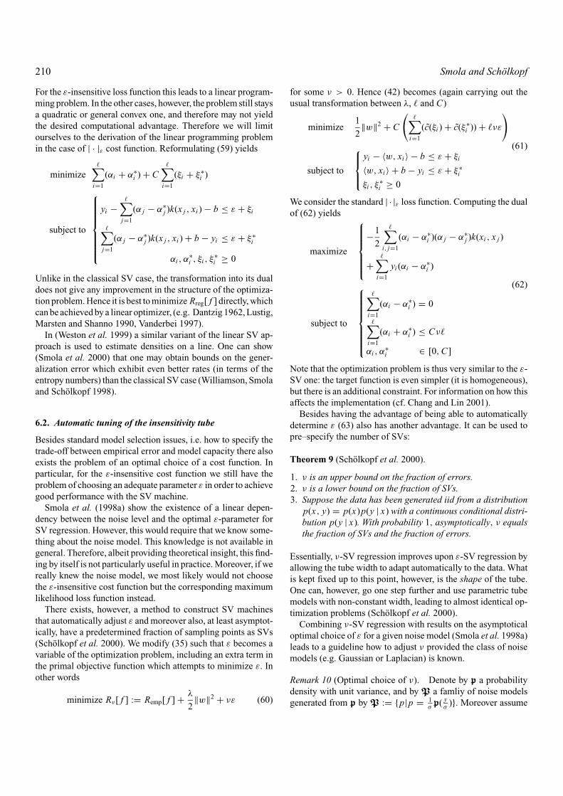
For the ε-insensitive loss function this leads to a linear program-ming problem. In the other cases, however, the problem still staysa quadratic or general convex one, and therefore may not yieldthe desired computational advantage. Therefore we will limitourselves to the derivation of the linear programming problemin the case of | · |ε cost function. Reformulating (59) yields
minimize�∑
i=1
(αi + α∗i ) + C
�∑i=1
(ξi + ξ ∗i )
subject to
yi −�∑
j=1
(α j − α∗j )k(x j , xi ) − b ≤ ε + ξi
�∑j=1
(α j − α∗j )k(x j , xi ) + b − yi ≤ ε + ξ ∗
i
αi , α∗i , ξi , ξ
∗i ≥ 0
Unlike in the classical SV case, the transformation into its dualdoes not give any improvement in the structure of the optimiza-tion problem. Hence it is best to minimize Rreg[ f ] directly, whichcan be achieved by a linear optimizer, (e.g. Dantzig 1962, Lustig,Marsten and Shanno 1990, Vanderbei 1997).
In (Weston et al. 1999) a similar variant of the linear SV ap-proach is used to estimate densities on a line. One can show(Smola et al. 2000) that one may obtain bounds on the gener-alization error which exhibit even better rates (in terms of theentropy numbers) than the classical SV case (Williamson, Smolaand Scholkopf 1998).
6.2. Automatic tuning of the insensitivity tube
Besides standard model selection issues, i.e. how to specify thetrade-off between empirical error and model capacity there alsoexists the problem of an optimal choice of a cost function. Inparticular, for the ε-insensitive cost function we still have theproblem of choosing an adequate parameter ε in order to achievegood performance with the SV machine.
Smola et al. (1998a) show the existence of a linear depen-dency between the noise level and the optimal ε-parameter forSV regression. However, this would require that we know some-thing about the noise model. This knowledge is not available ingeneral. Therefore, albeit providing theoretical insight, this find-ing by itself is not particularly useful in practice. Moreover, if wereally knew the noise model, we most likely would not choosethe ε-insensitive cost function but the corresponding maximumlikelihood loss function instead.
There exists, however, a method to construct SV machinesthat automatically adjust ε and moreover also, at least asymptot-ically, have a predetermined fraction of sampling points as SVs(Scholkopf et al. 2000). We modify (35) such that ε becomes avariable of the optimization problem, including an extra term inthe primal objective function which attempts to minimize ε. Inother words
minimize Rν[ f ] := Remp[ f ] + λ
2‖w‖2 + νε (60)
for some ν > 0. Hence (42) becomes (again carrying out theusual transformation between λ, � and C)
minimize1
2‖w‖2 + C
(�∑
i=1
(c(ξi ) + c(ξ ∗i )) + �νε
)(61)
subject to
yi − 〈w, xi 〉 − b ≤ ε + ξi
〈w, xi 〉 + b − yi ≤ ε + ξ ∗i
ξi , ξ∗i ≥ 0
We consider the standard | · |ε loss function. Computing the dualof (62) yields
maximize
−1
2
�∑i, j=1
(αi − α∗i )(α j − α∗
j )k(xi , x j )
+�∑
i=1
yi (αi − α∗i )
(62)
subject to
�∑i=1
(αi − α∗i ) = 0
�∑i=1
(αi + α∗i ) ≤ Cν�
αi , α∗i ∈ [0, C]
Note that the optimization problem is thus very similar to the ε-SV one: the target function is even simpler (it is homogeneous),but there is an additional constraint. For information on how thisaffects the implementation (cf. Chang and Lin 2001).
Besides having the advantage of being able to automaticallydetermine ε (63) also has another advantage. It can be used topre–specify the number of SVs:
Theorem 9 (Scholkopf et al. 2000).
1. ν is an upper bound on the fraction of errors.2. ν is a lower bound on the fraction of SVs.3. Suppose the data has been generated iid from a distribution
p(x, y) = p(x)p(y | x) with a continuous conditional distri-bution p(y | x). With probability 1, asymptotically, ν equalsthe fraction of SVs and the fraction of errors.
Essentially, ν-SV regression improves upon ε-SV regression byallowing the tube width to adapt automatically to the data. Whatis kept fixed up to this point, however, is the shape of the tube.One can, however, go one step further and use parametric tubemodels with non-constant width, leading to almost identical op-timization problems (Scholkopf et al. 2000).
Combining ν-SV regression with results on the asymptoticaloptimal choice of ε for a given noise model (Smola et al. 1998a)leads to a guideline how to adjust ν provided the class of noisemodels (e.g. Gaussian or Laplacian) is known.
Remark 10 (Optimal choice of ν). Denote by p a probabilitydensity with unit variance, and by P a famliy of noise modelsgenerated from p by P := {p|p = 1
σp( y
σ)}. Moreover assume

A tutorial on support vector regression 211
Fig. 5. Optimal ν and ε for various degrees of polynomial additivenoise
that the data were drawn iid from p(x, y) = p(x)p(y − f (x))with p(y − f (x)) continuous. Then under the assumption ofuniform convergence, the asymptotically optimal value of ν is
ν = 1 −∫ ε
−ε
p(t) dt
where ε := argminτ
(p(−τ ) + p(τ ))−2
(1 −
∫ τ
−τ
p(t) dt
)(63)
For polynomial noise models, i.e. densities of type exp(−|ξ |p)one may compute the corresponding (asymptotically) optimalvalues of ν. They are given in Fig. 5. For further details see(Scholkopf et al. 2000, Smola 1998); an experimental validationhas been given by Chalimourda, Scholkopf and Smola (2000).
We conclude this section by noting that ν-SV regression isrelated to the idea of trimmed estimators. One can show that theregression is not influenced if we perturb points lying outside thetube. Thus, the regression is essentially computed by discardinga certain fraction of outliers, specified by ν, and computing theregression estimate from the remaining points (Scholkopf et al.2000).
7. Regularization
So far we were not concerned about the specific properties ofthe map � into feature space and used it only as a convenienttrick to construct nonlinear regression functions. In some casesthe map was just given implicitly by the kernel, hence the mapitself and many of its properties have been neglected. A deeperunderstanding of the kernel map would also be useful to chooseappropriate kernels for a specific task (e.g. by incorporatingprior knowledge (Scholkopf et al. 1998a)). Finally the featuremap seems to defy the curse of dimensionality (Bellman 1961)
by making problems seemingly easier yet reliable via a map intosome even higher dimensional space.
In this section we focus on the connections between SVmethods and previous techniques like Regularization Networks(Girosi, Jones and Poggio 1993).9 In particular we will showthat SV machines are essentially Regularization Networks (RN)with a clever choice of cost functions and that the kernels areGreen’s function of the corresponding regularization operators.For a full exposition of the subject the reader is referred to Smola,Scholkopf and Muller (1998c).
7.1. Regularization networks
Let us briefly review the basic concepts of RNs. As in (35)we minimize a regularized risk functional. However, rather thanenforcing flatness in feature space we try to optimize somesmoothness criterion for the function in input space. Thus weget
Rreg[ f ] := Remp[ f ] + λ
2‖P f ‖2. (64)
Here P denotes a regularization operator in the sense ofTikhonov and Arsenin (1977), i.e. P is a positive semidefiniteoperator mapping from the Hilbert space H of functions f underconsideration to a dot product space D such that the expression〈P f · Pg〉 is well defined for f, g ∈ H . For instance by choos-ing a suitable operator that penalizes large variations of f onecan reduce the well–known overfitting effect. Another possiblesetting also might be an operator P mapping from L2(Rn) intosome Reproducing Kernel Hilbert Space (RKHS) (Aronszajn,1950, Kimeldorf and Wahba 1971, Saitoh 1988, Scholkopf 1997,Girosi 1998).
Using an expansion of f in terms of some symmetric functionk(xi , x j ) (note here, that k need not fulfill Mercer’s conditionand can be chosen arbitrarily since it is not used to define aregularization term),
f (x) =�∑
i=1
αi k(xi , x) + b, (65)
and the ε-insensitive cost function, this leads to a quadratic pro-gramming problem similar to the one for SVs. Using
Di j := 〈(Pk)(xi , .) · (Pk)(x j , .)〉 (66)
we get α = D−1 K (β − β∗), with β, β∗ being the solution of
minimize1
2(β∗ − β)�KD−1 K (β∗ − β)
−(β∗ − β)�y − ε
�∑i=1
(βi + β∗i ) (67)
subject to�∑
i=1
(βi − β∗i ) = 0 and βi , β
∗i ∈ [0, C].

212 Smola and Scholkopf
Unfortunately, this setting of the problem does not preserve spar-sity in terms of the coefficients, as a potentially sparse decom-position in terms of βi and β∗
i is spoiled by D−1 K , which is notin general diagonal.
7.2. Green’s functions
Comparing (10) with (67) leads to the question whether and un-der which condition the two methods might be equivalent andtherefore also under which conditions regularization networksmight lead to sparse decompositions, i.e. only a few of the ex-pansion coefficients αi in f would differ from zero. A sufficientcondition is D = K and thus KD−1 K = K (if K does not havefull rank we only need that KD−1 K = K holds on the image ofK ):
k(xi , x j ) = 〈(Pk)(xi , .) · (Pk)(x j , .)〉 (68)
Our goal now is to solve the following two problems:
1. Given a regularization operator P , find a kernel k such that aSV machine using k will not only enforce flatness in featurespace, but also correspond to minimizing a regularized riskfunctional with P as regularizer.
2. Given an SV kernel k, find a regularization operator P suchthat a SV machine using this kernel can be viewed as a Reg-ularization Network using P .
These two problems can be solved by employing the conceptof Green’s functions as described in Girosi, Jones and Poggio(1993). These functions were introduced for the purpose of solv-ing differential equations. In our context it is sufficient to knowthat the Green’s functions Gxi (x) of P∗ P satisfy
(P∗ PGxi )(x) = δxi (x). (69)
Here, δxi (x) is the δ-distribution (not to be confused with the Kro-necker symbol δi j ) which has the property that 〈 f ·δxi 〉 = f (xi ).The relationship between kernels and regularization operators isformalized in the following proposition:
Proposition 1 (Smola, Scholkopf and Muller 1998b). Let Pbe a regularization operator, and G be the Green’s function ofP∗ P. Then G is a Mercer Kernel such that D = K . SV machinesusing G minimize risk functional (64) with P as regularizationoperator.
In the following we will exploit this relationship in both ways:to compute Green’s functions for a given regularization operatorP and to infer the regularizer, given a kernel k.
7.3. Translation invariant kernels
Let us now more specifically consider regularization operatorsP that may be written as multiplications in Fourier space
〈P f · Pg〉 = 1
(2π )n/2
∫�
˜f (ω)g(ω)
P(ω)dω (70)
with ˜f (ω) denoting the Fourier transform of f (x), and P(ω) =P(−ω) real valued, nonnegative and converging to 0 for |ω| →∞ and � := supp[P(ω)]. Small values of P(ω) correspond toa strong attenuation of the corresponding frequencies. Hencesmall values of P(ω) for large ω are desirable since high fre-quency components of ˜f correspond to rapid changes in f .P(ω) describes the filter properties of P∗ P . Note that no atten-uation takes place for P(ω) = 0 as these frequencies have beenexcluded from the integration domain.
For regularization operators defined in Fourier Space by (70)one can show by exploiting P(ω) = P(−ω) = P(ω) that
G(xi , x) = 1
(2π )n/2
∫Rn
eiω(xi −x) P(ω) dω (71)
is a corresponding Green’s function satisfying translational in-variance, i.e.
G(xi , x j ) = G(xi − x j ) and G(ω) = P(ω). (72)
This provides us with an efficient tool for analyzing SV kernelsand the types of capacity control they exhibit. In fact the aboveis a special case of Bochner’s theorem (Bochner 1959) statingthat the Fourier transform of a positive measure constitutes apositive Hilbert Schmidt kernel.
Example 2 (Gaussian kernels). Following the exposition ofYuille and Grzywacz (1988) as described in Girosi, Jones andPoggio (1993), one can see that for
‖P f ‖2 =∫
dx∑
m
σ 2m
m!2m(Om f (x))2 (73)
with O2m = �m and O2m+1 = ∇�m , � being the Laplacianand ∇ the Gradient operator, we get Gaussians kernels (31).Moreover, we can provide an equivalent representation of Pin terms of its Fourier properties, i.e. P(ω) = e− σ2‖ω‖2
2 up to amultiplicative constant.
Training an SV machine with Gaussian RBF kernels (Scholkopfet al. 1997) corresponds to minimizing the specific cost func-tion with a regularization operator of type (73). Recall that (73)means that all derivatives of f are penalized (we have a pseudod-ifferential operator) to obtain a very smooth estimate. This alsoexplains the good performance of SV machines in this case, as itis by no means obvious that choosing a flat function in some highdimensional space will correspond to a simple function in lowdimensional space, as shown in Smola, Scholkopf and Muller(1998c) for Dirichlet kernels.
The question that arises now is which kernel to choose. Letus think about two extreme situations.
1. Suppose we already knew the shape of the power spectrumPow(ω) of the function we would like to estimate. In this casewe choose k such that k matches the power spectrum (Smola1998).
2. If we happen to know very little about the given data a gen-eral smoothness assumption is a reasonable choice. Hence

A tutorial on support vector regression 213
we might want to choose a Gaussian kernel. If computingtime is important one might moreover consider kernels withcompact support, e.g. using the Bq–spline kernels (cf. (32)).This choice will cause many matrix elements ki j = k(xi −x j )to vanish.
The usual scenario will be in between the two extreme cases andwe will have some limited prior knowledge available. For moreinformation on using prior knowledge for choosing kernels (seeScholkopf et al. 1998a).
7.4. Capacity control
All the reasoning so far was based on the assumption that thereexist ways to determine model parameters like the regularizationconstant λ or length scales σ of rbf–kernels. The model selec-tion issue itself would easily double the length of this reviewand moreover it is an area of active and rapidly moving research.Therefore we limit ourselves to a presentation of the basic con-cepts and refer the interested reader to the original publications.
It is important to keep in mind that there exist several fun-damentally different approaches such as Minimum DescriptionLength (cf. e.g. Rissanen 1978, Li and Vitanyi 1993) which isbased on the idea that the simplicity of an estimate, and thereforealso its plausibility is based on the information (number of bits)needed to encode it such that it can be reconstructed.
Bayesian estimation, on the other hand, considers the pos-terior probability of an estimate, given the observations X ={(x1, y1), . . . (x�, y�)}, an observation noise model, and a priorprobability distribution p( f ) over the space of estimates(parameters). It is given by Bayes Rule p( f | X )p(X ) =p(X | f )p( f ). Since p(X ) does not depend on f , one can maxi-mize p(X | f )p( f ) to obtain the so-called MAP estimate.10 Asa rule of thumb, to translate regularized risk functionals intoBayesian MAP estimation schemes, all one has to do is to con-sider exp(−Rreg[ f ]) = p( f | X ). For a more detailed discussion(see e.g. Kimeldorf and Wahba 1970, MacKay 1991, Neal 1996,Rasmussen 1996, Williams 1998).
A simple yet powerful way of model selection is cross valida-tion. This is based on the idea that the expectation of the erroron a subset of the training sample not used during training isidentical to the expected error itself. There exist several strate-gies such as 10-fold crossvalidation, leave-one out error (�-foldcrossvalidation), bootstrap and derived algorithms to estimatethe crossvalidation error itself (see e.g. Stone 1974, Wahba 1980,Efron 1982, Efron and Tibshirani 1994, Wahba 1999, Jaakkolaand Haussler 1999) for further details.
Finally, one may also use uniform convergence bounds suchas the ones introduced by Vapnik and Chervonenkis (1971). Thebasic idea is that one may bound with probability 1 − η (withη > 0) the expected risk R[ f ] by Remp[ f ] + �(F, η), where� is a confidence term depending on the class of functions F .Several criteria for measuring the capacity ofF exist, such as theVC-Dimension which, in pattern recognition problems, is givenby the maximum number of points that can be separated by the
function class in all possible ways, the Covering Number whichis the number of elements fromF that are needed to coverF withaccuracy of at least ε, Entropy Numbers which are the functionalinverse of Covering Numbers, and many more variants thereof(see e.g. Vapnik 1982, 1998, Devroye, Gyorfi and Lugosi 1996,Williamson, Smola and Scholkopf 1998, Shawe-Taylor et al.1998).
8. Conclusion
Due to the already quite large body of work done in the field ofSV research it is impossible to write a tutorial on SV regressionwhich includes all contributions to this field. This also wouldbe quite out of the scope of a tutorial and rather be relegated totextbooks on the matter (see Scholkopf and Smola (2002) for acomprehensive overview, Scholkopf, Burges and Smola (1999a)for a snapshot of the current state of the art, Vapnik (1998) for anoverview on statistical learning theory, or Cristianini and Shawe-Taylor (2000) for an introductory textbook). Still the authorshope that this work provides a not overly biased view of the stateof the art in SV regression research. We deliberately omitted(among others) the following topics.
8.1. Missing topics
Mathematical programming: Starting from a completely differ-ent perspective algorithms have been developed that are sim-ilar in their ideas to SV machines. A good primer mightbe (Bradley, Fayyad and Mangasarian 1998). (Also seeMangasarian 1965, 1969, Street and Mangasarian 1995). Acomprehensive discussion of connections between mathe-matical programming and SV machines has been given by(Bennett 1999).
Density estimation: with SV machines (Weston et al. 1999,Vapnik 1999). There one makes use of the fact that the cu-mulative distribution function is monotonically increasing,and that its values can be predicted with variable confidencewhich is adjusted by selecting different values of ε in the lossfunction.
Dictionaries: were originally introduced in the context ofwavelets by (Chen, Donoho and Saunders 1999) to allowfor a large class of basis functions to be considered simulta-neously, e.g. kernels with different widths. In the standard SVcase this is hardly possible except by defining new kernels aslinear combinations of differently scaled ones: choosing theregularization operator already determines the kernel com-pletely (Kimeldorf and Wahba 1971, Cox and O’Sullivan1990, Scholkopf et al. 2000). Hence one has to resort to lin-ear programming (Weston et al. 1999).
Applications: The focus of this review was on methods andtheory rather than on applications. This was done to limitthe size of the exposition. State of the art, or even recordperformance was reported in Muller et al. (1997), Druckeret al. (1997), Stitson et al. (1999) and Mattera and Haykin(1999).

214 Smola and Scholkopf
In many cases, it may be possible to achieve similar per-formance with neural network methods, however, only ifmany parameters are optimally tuned by hand, thus depend-ing largely on the skill of the experimenter. Certainly, SVmachines are not a “silver bullet.” However, as they haveonly few critical parameters (e.g. regularization and kernelwidth), state-of-the-art results can be achieved with relativelylittle effort.
8.2. Open issues
Being a very active field there exist still a number of open is-sues that have to be addressed by future research. After thatthe algorithmic development seems to have found a more sta-ble stage, one of the most important ones seems to be to findtight error bounds derived from the specific properties of ker-nel functions. It will be of interest in this context, whetherSV machines, or similar approaches stemming from a lin-ear programming regularizer, will lead to more satisfactoryresults.
Moreover some sort of “luckiness framework” (Shawe-Tayloret al. 1998) for multiple model selection parameters, similar tomultiple hyperparameters and automatic relevance detection inBayesian statistics (MacKay 1991, Bishop 1995), will have tobe devised to make SV machines less dependent on the skill ofthe experimenter.
It is also worth while to exploit the bridge between regulariza-tion operators, Gaussian processes and priors (see e.g. (Williams1998)) to state Bayesian risk bounds for SV machines in orderto compare the predictions with the ones from VC theory. Op-timization techniques developed in the context of SV machinesalso could be used to deal with large datasets in the Gaussianprocess settings.
Prior knowledge appears to be another important question inSV regression. Whilst invariances could be included in patternrecognition in a principled way via the virtual SV mechanismand restriction of the feature space (Burges and Scholkopf 1997,Scholkopf et al. 1998a), it is still not clear how (probably) moresubtle properties, as required for regression, could be dealt withefficiently.
Reduced set methods also should be considered for speedingup prediction (and possibly also training) phase for large datasets(Burges and Scholkopf 1997, Osuna and Girosi 1999, Scholkopfet al. 1999b, Smola and Scholkopf 2000). This topic is of greatimportance as data mining applications require algorithms thatare able to deal with databases that are often at least one order ofmagnitude larger (1 million samples) than the current practicalsize for SV regression.
Many more aspects such as more data dependent generaliza-tion bounds, efficient training algorithms, automatic kernel se-lection procedures, and many techniques that already have madetheir way into the standard neural networks toolkit, will have tobe considered in the future.
Readers who are tempted to embark upon a more detailedexploration of these topics, and to contribute their own ideas to
this exciting field, may find it useful to consult the web pagewww.kernel-machines.org.
Appendix A: Solving the interior-pointequations
A.1. Path following
Rather than trying to satisfy (53) directly we will solve a modifiedversion thereof for some µ > 0 substituted on the rhs in the firstplace and decrease µ while iterating.
gi zi = µ, si ti = µ for all i ∈ [1 . . . n]. (74)
Still it is rather difficult to solve the nonlinear system of equa-tions (51), (52), and (74) exactly. However we are not interestedin obtaining the exact solution to the approximation (74). In-stead, we seek a somewhat more feasible solution for a given µ,then decrease µ and repeat. This can be done by linearizing theabove system and solving the resulting equations by a predictor–corrector approach until the duality gap is small enough. Theadvantage is that we will get approximately equal performanceas by trying to solve the quadratic system directly, provided thatthe terms in �2 are small enough.
A(α + �α) = b
α + �α − g − �g = l
α + �α + t + �t = u
c + 1
2∂αq(α) + 1
2∂2αq(α)�α − (A(y + �y))�
+ s + �s = z + �z
(gi + �gi )(zi + �zi ) = µ
(si + �si )(ti + �ti ) = µ
Solving for the variables in � we get
A�α = b − Aα =: ρ
�α − �g = l − α + g =: ν
�α + �t = u − α − t =: τ
(A�y)� + �z − �s − 1
2∂2αq(α)�α
= c − (Ay)� + s − z + 1
2∂αq(α) =: σ
g−1z�g + �z = µg−1 − z − g−1�g�z =: γz
t−1s�t + �s = µt−1 − s − t−1�t�s =: γs
where g−1 denotes the vector (1/g1, . . . , 1/gn), and t analo-gously. Moreover denote g−1z and t−1s the vector generatedby the componentwise product of the two vectors. Solving for

A tutorial on support vector regression 215
�g, �t, �z, �s we get
�g = z−1g(γz − �z) �z = g−1z(ν − �α)
�t = s−1t(γs − �s) �s = t−1s(�α − τ )
where ν := ν − z−1gγz
τ := τ − s−1tγs
(75)
Now we can formulate the reduced KKT–system (see (Vanderbei1994) for the quadratic case):
[−H A�
A 0
][�α
�y
]=
[σ − g−1zν − t−1sτ
ρ
](76)
where H := ( 12∂2
αq(α) + g−1z + t−1s).
A.2. Iteration strategies
For the predictor-corrector method we proceed as follows. Inthe predictor step solve the system of (75) and (76) with µ = 0and all �-terms on the rhs set to 0, i.e. γz = z, γs = s. Thevalues in � are substituted back into the definitions for γz andγs and (75) and (76) are solved again in the corrector step. As thequadratic part in (76) is not affected by the predictor–correctorsteps, we only need to invert the quadratic matrix once. This isdone best by manually pivoting for the H part, as it is positivedefinite.
Next the values in�obtained by such an iteration step are usedto update the corresponding values in α, s, t, z, . . . . To ensurethat the variables meet the positivity constraints, the steplengthξ is chosen such that the variables move at most 1 − ε of theirinitial distance to the boundaries of the positive orthant. Usually(Vanderbei 1994) one sets ε = 0.05.
Another heuristic is used for computing µ, the parameter de-termining how much the KKT-conditions should be enforced.Obviously it is our aim to reduce µ as fast as possible, howeverif we happen to choose it too small, the condition of the equa-tions will worsen drastically. A setting that has proven to workrobustly is
µ = 〈g, z〉 + 〈s, t〉2n
(ξ − 1
ξ + 10
)2
. (77)
The rationale behind (77) is to use the average of the satisfac-tion of the KKT conditions (74) as point of reference and thendecrease µ rapidly if we are far enough away from the bound-aries of the positive orthant, to which all variables (except y) areconstrained to.
Finally one has to come up with good initial values. Analo-gously to Vanderbei (1994) we choose a regularized version of(76) in order to determine the initial conditions. One solves[
−(12∂2
αq(α) + 1)
A�
A 1
] [α
y
]=
[c
b
](78)
and subsequently restricts the solution to a feasible set
x = max
(x,
u
100
)g = min(α − l, u)
t = min(u − α, u) (79)
z = min
(�
(1
2∂αq(α) + c − (Ay)�
)+ u
100, u
)
s = min
(�
(−1
2∂αq(α) − c + (Ay)�
)+ u
100, u
)
�(·) denotes the Heavyside function, i.e. �(x) = 1 for x > 0and �(x) = 0 otherwise.
A.3. Special considerations for SV regression
The algorithm described so far can be applied to both SV patternrecognition and regression estimation. For the standard settingin pattern recognition we have
q(α) =�∑
i, j=0
αiα j yi y j k(xi , x j ) (80)
and consequently ∂αi q(α) = 0, ∂2αi α j
q(α) = yi y j k(xi , x j ), i.e.the Hessian is dense and the only thing we can do is computeits Cholesky factorization to compute (76). In the case of SV re-gression, however we have (with α := (α1, . . . , α�, α
∗1 , . . . , α
∗� ))
q(α) =�∑
i, j=1
(αi − α∗i )(α j − α∗
j )k(xi , x j )
+ 2C�∑
i=1
T (αi ) + T (α∗i ) (81)
and therefore
∂αi q(α) = d
dαiT (αi )
∂2αi α j
q(α) = k(xi , x j ) + δi jd2
dα2i
T (αi ) (82)
∂2αi α
∗jq(α) = −k(xi , x j )
and ∂2α∗
i α∗jq(α), ∂2
α∗i α j
q(α) analogously. Hence we are dealing witha matrix of type M := [ K+D −K−K K+D′ ] where D, D′ are diagonalmatrices. By applying an orthogonal transformation M can beinverted essentially by inverting an � × � matrix instead of a2� × 2� system. This is exactly the additional advantage onecan gain from implementing the optimization algorithm directlyinstead of using a general purpose optimizer. One can show thatfor practical implementations (Smola, Scholkopf and Muller1998b) one can solve optimization problems using nearly ar-bitrary convex cost functions as efficiently as the special case ofε-insensitive loss functions.
Finally note that due to the fact that we are solving the pri-mal and dual optimization problem simultaneously we are also

216 Smola and Scholkopf
computing parameters corresponding to the initial SV optimiza-tion problem. This observation is useful as it allows us to obtainthe constant term b directly, namely by setting b = y. (see Smola(1998) for details).
Appendix B: Solving the subset selectionproblem
B.1. Subset optimization problem
We will adapt the exposition of Joachims (1999) to the case ofregression with convex cost functions. Without loss of general-ity we will assume ε �= 0 and α ∈ [0, C] (the other situationscan be treated as a special case). First we will extract a reducedoptimization problem for the working set when all other vari-ables are kept fixed. Denote Sw ⊂ {1, . . . , �} the working setand S f := {1, . . . , �}\Sw the fixed set. Writing (43) as an opti-mization problem only in terms of Sw yields
maximize
−1
2
∑i, j∈Sw
(αi − α∗i )(α j − α∗
j )〈xi , x j 〉
+∑i∈Sw
(αi − α∗i )
(yi −
∑j∈S f
(α j − α∗j )〈xi , x j 〉
)
+∑i∈Sw
(−ε(αi + α∗i ) + C(T (αi ) + T (α∗
i )))
subject to
∑i∈Sw
(αi − α∗i ) = −
∑i∈S f
(αi − α∗i )
αi ∈ [0, C]
(83)
Hence we only have to update the linear term by the couplingwith the fixed set − ∑
i∈Sw(αi −α∗
i )∑
j∈S f(α j −α∗
j )〈xi , x j 〉 andthe equality constraint by − ∑
i∈S f(αi − α∗
i ). It is easy to seethat maximizing (83) also decreases (43) by exactly the sameamount. If we choose variables for which the KKT–conditionsare not satisfied the overall objective function tends to decreasewhilst still keeping all variables feasible. Finally it is boundedfrom below.
Even though this does not prove convergence (contrary tostatement in Osuna, Freund and Girosi (1997)) this algorithmproves very useful in practice. It is one of the few methods (be-sides (Kaufman 1999, Platt 1999)) that can deal with problemswhose quadratic part does not completely fit into memory. Stillin practice one has to take special precautions to avoid stallingof convergence (recent results of Chang, Hsu and Lin (1999)indicate that under certain conditions a proof of convergence ispossible). The crucial part is the one of Sw.
B.2. A note on optimality
For convenience the KKT conditions are repeated in a slightlymodified form. Denote ϕi the error made by the current estimate
at sample xi , i.e.
ϕi := yi − f (xi ) = yi −[
m∑j=1
k(xi , x j )(αi − α∗i ) + b
]. (84)
Rewriting the feasibility conditions (52) in terms of α yields
2∂αi T (αi ) + ε − ϕi + si − zi = 0(85)
2∂α∗iT (α∗
i ) + ε + ϕi + s∗i − z∗
i = 0
for all i ∈ {1, . . . , m} with zi , z∗i , si , s∗
i ≥ 0. A set of dualfeasible variables z, s is given by
zi = max(2∂αi T (αi ) + ε − ϕi , 0
)si = − min
(2∂αi T (αi ) + ε − ϕi , 0
)(86)
z∗i = max
(2∂α∗
iT (α∗
i ) + ε + ϕi , 0)
s∗i = − min
(2∂α∗
iT (α∗
i ) + ε + ϕi , 0)
Consequently the KKT conditions (53) can be translated into
αi zi = 0 and (C − αi )si = 0(87)
α∗i z∗
i = 0 and (C − α∗i )s∗
i = 0
All variables αi , α∗i violating some of the conditions of (87) may
be selected for further optimization. In most cases, especially inthe initial stage of the optimization algorithm, this set of pat-terns is much larger than any practical size of Sw. UnfortunatelyOsuna, Freund and Girosi (1997) contains little information onhow to select Sw. The heuristics presented here are an adaptationof Joachims (1999) to regression. See also Lin (2001) for detailson optimization for SVR.
B.3. Selection rules
Similarly to a merit function approach (El-Bakry et al. 1996) theidea is to select those variables that violate (85) and (87) most,thus contribute most to the feasibility gap. Hence one defines ascore variable ζi by
ζi := gi zi + si ti
= αi zi + α∗i z∗
i + (C − αi )si + (C − α∗i )s∗
i (88)
By construction,∑
i ζi is the size of the feasibility gap (cf. (56)for the case of ε-insensitive loss). By decreasing this gap, oneapproaches the the solution (upper bounded by the primal objec-tive and lower bounded by the dual objective function). Hence,the selection rule is to choose those patterns for which ζi is

A tutorial on support vector regression 217
largest. Some algorithms use
ζ ′i := αi�(zi ) + α∗
i �(z∗i )
+ (C − αi )�(si ) + (C − α∗i )�(si )
(89)or ζ ′′
i := �(αi )zi + �(α∗i )z∗
i
+ �(C − αi )si + �(C − α∗i )si .
One can see that ζi = 0, ζ ′i = 0, and ζ ′′
i = 0 mutually imply eachother. However, only ζi gives a measure for the contribution ofthe variable i to the size of the feasibility gap.
Finally, note that heuristics like assigning sticky–flags (cf.Burges 1998) to variables at the boundaries, thus effec-tively solving smaller subproblems, or completely removingthe corresponding patterns from the training set while ac-counting for their couplings (Joachims 1999) can signifi-cantly decrease the size of the problem one has to solve andthus result in a noticeable speedup. Also caching (Joachims1999, Kowalczyk 2000) of already computed entries of thedot product matrix may have a significant impact on theperformance.
Appendix C: Solving the SMO equations
C.1. Pattern dependent regularization
Consider the constrained optimization problem (83) for two in-dices, say (i, j). Pattern dependent regularization means that Ci
may be different for every pattern (possibly even different forαi and α∗
i ). Since at most two variables may become nonzeroat the same time and moreover we are dealing with a con-strained optimization problem we may express everything interms of just one variable. From the summation constraint weobtain
(αi − α∗i ) + (α j − α∗
j ) = (αold
i − α∗i
old) + (αold
j − α∗jold) := γ
(90)
for regression. Exploiting α(∗)j ∈ [0, C (∗)
j ] yields α(∗)i ∈ [L , H ].
This is taking account of the fact that there may be only fourdifferent pairs of nonzero variables: (αi , α j ), (α∗
i , α j ), (αi , α∗j ),
and (α∗i , α
∗j ). For convenience define an auxiliary variables s
such that s = 1 in the first and the last case and s = −1 other-wise.
α j α∗j
αi L max(0, γ − C j ) max(0, γ )H min(Ci , γ ) min(Ci , C∗
j + γ )α∗
i L max(0, −γ ) max(0, −γ − C∗j )
H min(C∗i , −γ + C j ) min(C∗
i , −γ )
C.2. Analytic solution for regression
Next one has to solve the optimization problem analytically. Wemake use of (84) and substitute the values of φi into the reducedoptimization problem (83). In particular we use
yi −∑j �∈Sw
(αi − α∗i )Ki j = ϕi + b +
∑j∈Sw
(αold
i − α∗i
old)Ki j .
(91)
Moreover with the auxiliary variables γ = αi −α∗i +α j −α∗
j andη := (Kii + K j j − 2Ki j ) one obtains the following constrainedoptimization problem in i (after eliminating j , ignoring termsindependent of α j , α
∗j and noting that this only holds for αiα
∗i =
α jα∗j = 0):
maximize − 1
2(αi − α∗
i )2η − ε(αi + α∗i )(1 − s)
+ (αi − α∗i )
(φi − φ j + η
(αold
i − α∗i
old)) (92)
subject to α(∗)i ∈ [L (∗), H (∗)].
The unconstrained maximum of (92) with respect to αi or α∗i
can be found below.
(I) αi , α j αoldi + η−1(ϕi − ϕ j )
(II) αi , α∗j αold
i + η−1(ϕi − ϕ j − 2ε)(III) α∗
i , α j α∗i
old − η−1(ϕi − ϕ j + 2ε)(IV) α∗
i , α∗j α∗
iold − η−1(ϕi − ϕ j )
The problem is that we do not know beforehand which of thefour quadrants (I)–(IV) contains the solution. However, by con-sidering the sign of γ we can distinguish two cases: for γ > 0only (I)–(III) are possible, for γ < 0 the coefficients satisfy oneof the cases (II)–(IV). In case of γ = 0 only (II) and (III) haveto be considered. See also the diagram below.
For γ > 0 it is best to start with quadrant (I), test whether theunconstrained solution hits one of the boundaries L , H and if so,probe the corresponding adjacent quadrant (II) or (III). γ < 0can be dealt with analogously.
Due to numerical instabilities, it may happen that η < 0. Inthat case η should be set to 0 and one has to solve (92) in a linearfashion directly.11

218 Smola and Scholkopf
C.3. Selection rule for regression
Finally, one has to pick indices (i, j) such that the objectivefunction is maximized. Again, the reasoning of SMO (Platt 1999,Section 12.2.2) for classification will be mimicked. This meansthat a two loop approach is chosen to maximize the objectivefunction. The outer loop iterates over all patterns violating theKKT conditions, first only over those with Lagrange multipliersneither on the upper nor lower boundary, and once all of themare satisfied, over all patterns violating the KKT conditions, toensure self consistency on the complete dataset.12 This solvesthe problem of choosing i .
Now for j : To make a large step towards the minimum, onelooks for large steps in αi . As it is computationally expensive tocompute η for all possible pairs (i, j) one chooses the heuristic tomaximize the absolute value of the numerator in the expressionsfor αi and α∗
i , i.e. |ϕi − ϕ j | and |ϕi − ϕ j ± 2ε|. The index jcorresponding to the maximum absolute value is chosen for thispurpose.
If this heuristic happens to fail, in other words if little progressis made by this choice, all other indices j are looked at (this iswhat is called “second choice hierarcy” in Platt (1999) in thefollowing way:
1. All indices j corresponding to non–bound examples arelooked at, searching for an example to make progress on.
2. In the case that the first heuristic was unsuccessful, allother samples are analyzed until an example is found whereprogress can be made.
3. If both previous steps fail proceed to the next i .
For a more detailed discussion (see Platt 1999). Unlike interiorpoint algorithms SMO does not automatically provide a valuefor b. However this can be chosen like in Section 1.4 by havinga close look at the Lagrange multipliers α
(∗)i obtained.
C.4. Stopping criteria
By essentially minimizing a constrained primal optimizationproblem one cannot ensure that the dual objective function in-creases with every iteration step.13 Nevertheless one knows thatthe minimum value of the objective function lies in the interval[dual objectivei , primal objectivei ] for all steps i , hence also inthe interval [(max j≤i dual objective j ), primal objectivei ]. Oneuses the latter to determine the quality of the current solution.
The calculation of the primal objective function from the pre-diction errors is straightforward. One uses
∑i, j
(αi − α∗i )(α j − α∗
j )ki j = −∑
i
(αi − α∗i )(ϕi + yi − b),
(93)
i.e. the definition of ϕi to avoid the matrix–vector multiplicationwith the dot product matrix.
Acknowledgments
This work has been supported in part by a grant of the DFG(Ja 379/71, Sm 62/1). The authors thank Peter Bartlett, ChrisBurges, Stefan Harmeling, Olvi Mangasarian, Klaus-RobertMuller, Vladimir Vapnik, Jason Weston, Robert Williamson, andAndreas Ziehe for helpful discussions and comments.
Notes
1. Our use of the term ‘regression’ is somewhat lose in that it also includescases of function estimation where one minimizes errors other than the meansquare loss. This is done mainly for historical reasons (Vapnik, Golowichand Smola 1997).
2. A similar approach, however using linear instead of quadratic programming,was taken at the same time in the USA, mainly by Mangasarian (1965, 1968,1969).
3. See Smola (1998) for an overview over other ways of specifying flatness ofsuch functions.
4. This is true as long as the dimensionality of w is much higher than thenumber of observations. If this is not the case, specialized methods canoffer considerable computational savings (Lee and Mangasarian 2001).
5. The table displays CT(α) instead of T (α) since the former can be pluggeddirectly into the corresponding optimization equations.
6. The high price tag usually is the major deterrent for not using them. Moreoverone has to bear in mind that in SV regression, one may speed up the solutionconsiderably by exploiting the fact that the quadratic form has a specialstructure or that there may exist rank degeneracies in the kernel matrixitself.
7. For large and noisy problems (e.g. 100.000 patterns and more with a substan-tial fraction of nonbound Lagrange multipliers) it is impossible to solve theproblem exactly: due to the size one has to use subset selection algorithms,hence joint optimization over the training set is impossible. However, unlikein Neural Networks, we can determine the closeness to the optimum. Notethat this reasoning only holds for convex cost functions.
8. A similar technique was employed by Bradley and Mangasarian (1998) inthe context of linear programming in order to deal with large datasets.
9. Due to length constraints we will not deal with the connection betweenGaussian Processes and SVMs. See Williams (1998) for an excellentoverview.
10. Strictly speaking, in Bayesian estimation one is not so much concerned aboutthe maximizer ˆf of p( f | X ) but rather about the posterior distribution off .
11. Negative values of η are theoretically impossible since k satisfies Mercer’scondition: 0 ≤ ‖�(xi ) − �(x j )‖2 = Kii + K j j − 2Ki j = η.
12. It is sometimes useful, especially when dealing with noisy data, to iterateover the complete KKT violating dataset already before complete self con-sistency on the subset has been achieved. Otherwise much computationalresources are spent on making subsets self consistent that are not globallyself consistent. This is the reason why in the pseudo code a global loopis initiated already when only less than 10% of the non bound variableschanged.
13. It is still an open question how a subset selection optimization algorithmcould be devised that decreases both primal and dual objective functionat the same time. The problem is that this usually involves a number ofdual variables of the order of the sample size, which makes this attemptunpractical.
References
Aizerman M.A., Braverman E.M., and Rozonoer L.I. 1964. Theoreticalfoundations of the potential function method in pattern recognitionlearning. Automation and Remote Control 25: 821–837.
Aronszajn N. 1950. Theory of reproducing kernels. Transactions of theAmerican Mathematical Society 68: 337–404.

A tutorial on support vector regression 219
Bazaraa M.S., Sherali H.D., and Shetty C.M. 1993. Nonlinear Program-ming: Theory and Algorithms, 2nd edition, Wiley.
Bellman R.E. 1961. Adaptive Control Processes. Princeton UniversityPress, Princeton, NJ.
Bennett K. 1999. Combining support vector and mathematical program-ming methods for induction. In: Scholkopf B., Burges C.J.C., andSmola A.J., (Eds.), Advances in Kernel Methods—SV Learning,MIT Press, Cambridge, MA, pp. 307–326.
Bennett K.P. and Mangasarian O.L. 1992. Robust linear program-ming discrimination of two linearly inseparable sets. OptimizationMethods and Software 1: 23–34.
Berg C., Christensen J.P.R., and Ressel P. 1984. Harmonic Analysis onSemigroups. Springer, New York.
Bertsekas D.P. 1995. Nonlinear Programming. Athena Scientific,Belmont, MA.
Bishop C.M. 1995. Neural Networks for Pattern Recognition.Clarendon Press, Oxford.
Blanz V., Scholkopf B., Bulthoff H., Burges C., Vapnik V., and VetterT. 1996. Comparison of view-based object recognition algorithmsusing realistic 3D models. In: von der Malsburg C., von SeelenW., Vorbruggen J.C., and Sendhoff B. (Eds.), Artificial NeuralNetworks ICANN’96, Berlin. Springer Lecture Notes in ComputerScience, Vol. 1112, pp. 251–256.
Bochner S. 1959. Lectures on Fourier integral. Princeton Univ. Press,Princeton, New Jersey.
Boser B.E., Guyon I.M., and Vapnik V.N. 1992. A training algorithm foroptimal margin classifiers. In: Haussler D. (Ed.), Proceedings ofthe Annual Conference on Computational Learning Theory. ACMPress, Pittsburgh, PA, pp. 144–152.
Bradley P.S., Fayyad U.M., and Mangasarian O.L. 1998. Data min-ing: Overview and optimization opportunities. Technical Re-port 98–01, University of Wisconsin, Computer Sciences Depart-ment, Madison, January. INFORMS Journal on Computing, toappear.
Bradley P.S. and Mangasarian O.L. 1998. Feature selection via con-cave minimization and support vector machines. In: Shavlik J.(Ed.), Proceedings of the International Conference on MachineLearning, Morgan Kaufmann Publishers, San Francisco, Califor-nia, pp. 82–90. ftp://ftp.cs.wisc.edu/math-prog/tech-reports/98-03.ps.Z.
Bunch J.R. and Kaufman L. 1977. Some stable methods for calculat-ing inertia and solving symmetric linear systems. Mathematics ofComputation 31: 163–179.
Bunch J.R. and Kaufman L. 1980. A computational method for theindefinite quadratic programming problem. Linear Algebra andIts Applications, pp. 341–370, December.
Bunch J.R., Kaufman L., and Parlett B. 1976. Decomposition of a sym-metric matrix. Numerische Mathematik 27: 95–109.
Burges C.J.C. 1996. Simplified support vector decision rules. InL. Saitta (Ed.), Proceedings of the International Conference onMachine Learning, Morgan Kaufmann Publishers, San Mateo,CA, pp. 71–77.
Burges C.J.C. 1998. A tutorial on support vector machines for patternrecognition. Data Mining and Knowledge Discovery 2(2): 121–167.
Burges C.J.C. 1999. Geometry and invariance in kernel based methods.In Scholkopf B., Burges C.J.C., and Smola A.J., (Eds.), Advancesin Kernel Methods—Support Vector Learning, MIT Press, Cam-bridge, MA, pp. 89–116.
Burges C.J.C. and Scholkopf B. 1997. Improving the accuracy and speedof support vector learning machines. In Mozer M.C., Jordan M.I.,and Petsche T., (Eds.), Advances in Neural Information ProcessingSystems 9, MIT Press, Cambridge, MA, pp. 375–381.
Chalimourda A., Scholkopf B., and Smola A.J. 2004. Experimentallyoptimal ν in support vector regression for different noise modelsand parameter settings. Neural Networks 17(1): 127–141.
Chang C.-C., Hsu C.-W., and Lin C.-J. 1999. The analysis of decom-position methods for support vector machines. In Proceeding ofIJCAI99, SVM Workshop.
Chang C.C. and Lin C.J. 2001. Training ν-support vector classi-fiers: Theory and algorithms. Neural Computation 13(9): 2119–2147.
Chen S., Donoho D., and Saunders M. 1999. Atomic decomposition bybasis pursuit. Siam Journal of Scientific Computing 20(1): 33–61.
Cherkassky V. and Mulier F. 1998. Learning from Data. John Wiley andSons, New York.
Cortes C. and Vapnik V. 1995. Support vector networks. Machine Learn-ing 20: 273–297.
Cox D. and O’Sullivan F. 1990. Asymptotic analysis of penalized like-lihood and related estimators. Annals of Statistics 18: 1676–1695.
CPLEX Optimization Inc. Using the CPLEX callable library. Manual,1994.
Cristianini N. and Shawe-Taylor J. 2000. An Introduction to SupportVector Machines. Cambridge University Press, Cambridge, UK.
Cristianini N., Campbell C., and Shawe-Taylor J. 1998. Multiplicativeupdatings for support vector learning. NeuroCOLT Technical Re-port NC-TR-98-016, Royal Holloway College.
Dantzig G.B. 1962. Linear Programming and Extensions. PrincetonUniv. Press, Princeton, NJ.
Devroye L., Gyorfi L., and Lugosi G. 1996. A Probabilistic Theory ofPattern Recognition. Number 31 in Applications of mathematics.Springer, New York.
Drucker H., Burges C.J.C., Kaufman L., Smola A., and Vapnik V. 1997.Support vector regression machines. In: Mozer M.C., Jordan M.I.,and Petsche T. (Eds.), Advances in Neural Information ProcessingSystems 9, MIT Press, Cambridge, MA, pp. 155–161.
Efron B. 1982. The jacknife, the bootstrap, and other resampling plans.SIAM, Philadelphia.
Efron B. and Tibshirani R.J. 1994. An Introduction to the Bootstrap.Chapman and Hall, New York.
El-Bakry A., Tapia R., Tsuchiya R., and Zhang Y. 1996. On the formula-tion and theory of the Newton interior-point method for nonlinearprogramming. J. Optimization Theory and Applications 89: 507–541.
Fletcher R. 1989. Practical Methods of Optimization. John Wiley andSons, New York.
Girosi F. 1998. An equivalence between sparse approximation and sup-port vector machines. Neural Computation 10(6): 1455–1480.
Girosi F., Jones M., and Poggio T. 1993. Priors, stabilizers and ba-sis functions: From regularization to radial, tensor and additivesplines. A.I. Memo No. 1430, Artificial Intelligence Laboratory,Massachusetts Institute of Technology.
Guyon I., Boser B., and Vapnik V. 1993. Automatic capacity tuning ofvery large VC-dimension classifiers. In: Hanson S.J., Cowan J.D.,and Giles C.L. (Eds.), Advances in Neural Information ProcessingSystems 5. Morgan Kaufmann Publishers, pp. 147–155.
Hardle W. 1990. Applied nonparametric regression, volume 19 ofEconometric Society Monographs. Cambridge University Press.

220 Smola and Scholkopf
Hastie T.J. and Tibshirani R.J. 1990. Generalized Additive Models,volume 43 of Monographs on Statistics and Applied Probability.Chapman and Hall, London.
Haykin S. 1998. Neural Networks: A Comprehensive Foundation. 2ndedition. Macmillan, New York.
Hearst M.A., Scholkopf B., Dumais S., Osuna E., and Platt J. 1998.Trends and controversies—support vector machines. IEEE Intel-ligent Systems 13: 18–28.
Herbrich R. 2002. Learning Kernel Classifiers: Theory and Algorithms.MIT Press.
Huber P.J. 1972. Robust statistics: A review. Annals of Statistics43: 1041.
Huber P.J. 1981. Robust Statistics. John Wiley and Sons, New York.IBM Corporation. 1992. IBM optimization subroutine library guide
and reference. IBM Systems Journal, 31, SC23-0519.Jaakkola T.S. and Haussler D. 1999. Probabilistic kernel regression
models. In: Proceedings of the 1999 Conference on AI and Statis-tics.
Joachims T. 1999. Making large-scale SVM learning practical.In: Scholkopf B., Burges C.J.C., and Smola A.J. (Eds.), Ad-vances in Kernel Methods—Support Vector Learning, MIT Press,Cambridge, MA, pp. 169–184.
Karush W. 1939. Minima of functions of several variables with inequal-ities as side constraints. Master’s thesis, Dept. of Mathematics,Univ. of Chicago.
Kaufman L. 1999. Solving the quadratic programming problem arisingin support vector classification. In: Scholkopf B., Burges C.J.C.,and Smola A.J. (Eds.), Advances in Kernel Methods—SupportVector Learning, MIT Press, Cambridge, MA, pp. 147–168
Keerthi S.S., Shevade S.K., Bhattacharyya C., and Murthy K.R.K. 1999.Improvements to Platt’s SMO algorithm for SVM classifier design.Technical Report CD-99-14, Dept. of Mechanical and ProductionEngineering, Natl. Univ. Singapore, Singapore.
Keerthi S.S., Shevade S.K., Bhattacharyya C., and Murty K.R.K. 2001.Improvements to platt’s SMO algorithm for SVM classifier design.Neural Computation 13: 637–649.
Kimeldorf G.S. and Wahba G. 1970. A correspondence betweenBayesian estimation on stochastic processes and smoothing bysplines. Annals of Mathematical Statistics 41: 495–502.
Kimeldorf G.S. and Wahba G. 1971. Some results on Tchebycheffianspline functions. J. Math. Anal. Applic. 33: 82–95.
Kowalczyk A. 2000. Maximal margin perceptron. In: Smola A.J.,Bartlett P.L., Scholkopf B., and Schuurmans D. (Eds.), Advancesin Large Margin Classifiers, MIT Press, Cambridge, MA, pp. 75–113.
Kuhn H.W. and Tucker A.W. 1951. Nonlinear programming. In: Proc.2nd Berkeley Symposium on Mathematical Statistics and Proba-bilistics, Berkeley. University of California Press, pp. 481–492.
Lee Y.J. and Mangasarian O.L. 2001. SSVM: A smooth support vectormachine for classification. Computational optimization and Ap-plications 20(1): 5–22.
Li M. and Vitanyi P. 1993. An introduction to Kolmogorov Complexityand its applications. Texts and Monographs in Computer Science.Springer, New York.
Lin C.J. 2001. On the convergence of the decomposition method forsupport vector machines. IEEE Transactions on Neural Networks12(6): 1288–1298.
Lustig I.J., Marsten R.E., and Shanno D.F. 1990. On implementingMehrotra’s predictor-corrector interior point method for linear pro-
gramming. Princeton Technical Report SOR 90–03., Dept. of CivilEngineering and Operations Research, Princeton University.
Lustig I.J., Marsten R.E., and Shanno D.F. 1992. On implement-ing Mehrotra’s predictor-corrector interior point method for lin-ear programming. SIAM Journal on Optimization 2(3): 435–449.
MacKay D.J.C. 1991. Bayesian Methods for Adaptive Models. PhDthesis, Computation and Neural Systems, California Institute ofTechnology, Pasadena, CA.
Mangasarian O.L. 1965. Linear and nonlinear separation of patterns bylinear programming. Operations Research 13: 444–452.
Mangasarian O.L. 1968. Multi-surface method of pattern separation.IEEE Transactions on Information Theory IT-14: 801–807.
Mangasarian O.L. 1969. Nonlinear Programming. McGraw-Hill, NewYork.
Mattera D. and Haykin S. 1999. Support vector machines for dy-namic reconstruction of a chaotic system. In: Scholkopf B., BurgesC.J.C., and Smola A.J. (Eds.), Advances in Kernel Methods—Support Vector Learning, MIT Press, Cambridge, MA, pp. 211–242.
McCormick G.P. 1983. Nonlinear Programming: Theory, Algorithms,and Applications. John Wiley and Sons, New York.
Megiddo N. 1989. Progressin Mathematical Programming, chapterPathways to the optimal set in linear programming, Springer, NewYork, NY, pp. 131–158.
Mehrotra S. and Sun J. 1992. On the implementation of a (primal-dual)interior point method. SIAM Journal on Optimization 2(4): 575–601.
Mercer J. 1909. Functions of positive and negative type and their con-nection with the theory of integral equations. Philosophical Trans-actions of the Royal Society, London A 209: 415–446.
Micchelli C.A. 1986. Algebraic aspects of interpolation. Proceedingsof Symposia in Applied Mathematics 36: 81–102.
Morozov V.A. 1984. Methods for Solving Incorrectly Posed Problems.Springer.
Muller K.-R., Smola A., Ratsch G., Scholkopf B., Kohlmorgen J., andVapnik V. 1997. Predicting time series with support vector ma-chines. In: Gerstner W., Germond A., Hasler M., and Nicoud J.-D.(Eds.), Artificial Neural Networks ICANN’97, Berlin. SpringerLecture Notes in Computer Science Vol. 1327 pp. 999–1004.
Murtagh B.A. and Saunders M.A. 1983. MINOS 5.1 user’s guide. Tech-nical Report SOL 83-20R, Stanford University, CA, USA, Revised1987.
Neal R. 1996. Bayesian Learning in Neural Networks. Springer.Nilsson N.J. 1965. Learning machines: Foundations of Trainable Pattern
Classifying Systems. McGraw-Hill.Nyquist. H. 1928. Certain topics in telegraph transmission theory.
Trans. A.I.E.E., pp. 617–644.Osuna E., Freund R., and Girosi F. 1997. An improved training algo-
rithm for support vector machines. In Principe J., Gile L., MorganN., and Wilson E. (Eds.), Neural Networks for Signal ProcessingVII—Proceedings of the 1997 IEEE Workshop, pp. 276–285, NewYork, IEEE.
Osuna E. and Girosi F. 1999. Reducing the run-time complexity insupport vector regression. In: Scholkopf B., Burges C.J.C., andSmola A. J. (Eds.), Advances in Kernel Methods—Support VectorLearning, pp. 271–284, Cambridge, MA, MIT Press.
Ovari Z. 2000. Kernels, eigenvalues and support vector machines. Hon-ours thesis, Australian National University, Canberra.

A tutorial on support vector regression 221
Platt J. 1999. Fast training of support vector machines using sequen-tial minimal optimization. In: Scholkopf B., Burges C.J.C., andSmola A.J. (Eds.) Advances in Kernel Methods—Support VectorLearning, pp. 185–208, Cambridge, MA, MIT Press.
Poggio T. 1975. On optimal nonlinear associative recall. BiologicalCybernetics, 19: 201–209.
Rasmussen C. 1996. Evaluation of Gaussian Processes andOther Methods for Non-Linear Regression. PhD thesis,Department of Computer Science, University of Toronto,ftp://ftp.cs.toronto.edu/pub/carl/thesis.ps.gz.
Rissanen J. 1978. Modeling by shortest data description. Automatica,14: 465–471.
Saitoh S. 1988. Theory of Reproducing Kernels and its Applications.Longman Scientific & Technical, Harlow, England.
Saunders C., Stitson M.O., Weston J., Bottou L., Scholkopf B., andSmola A. 1998. Support vector machine—reference manual. Tech-nical Report CSD-TR-98-03, Department of Computer Science,Royal Holloway, University of London, Egham, UK. SVM avail-able at http://svm.dcs.rhbnc.ac.uk/.
Schoenberg I. 1942. Positive definite functions on spheres. DukeMath. J., 9: 96–108.
Scholkopf B. 1997. Support Vector Learning. R. OldenbourgVerlag, Munchen. Doktorarbeit, TU Berlin. Download:http://www.kernel-machines.org.
Scholkopf B., Burges C., and Vapnik V. 1995. Extracting support datafor a given task. In: Fayyad U.M. and Uthurusamy R. (Eds.), Pro-ceedings, First International Conference on Knowledge Discovery& Data Mining, Menlo Park, AAAI Press.
Scholkopf B., Burges C., and Vapnik V. 1996. Incorporating invariancesin support vector learning machines. In: von der Malsburg C., vonSeelen W., Vorbruggen J. C., and Sendhoff B. (Eds.), ArtificialNeural Networks ICANN’96, pp. 47–52, Berlin, Springer LectureNotes in Computer Science, Vol. 1112.
Scholkopf B., Burges C.J.C., and Smola A.J. 1999a. (Eds.) Ad-vances in Kernel Methods—Support Vector Learning. MIT Press,Cambridge, MA.
Scholkopf B., Herbrich R., Smola A.J., and Williamson R.C. 2001. Ageneralized representer theorem. Technical Report 2000-81, Neu-roCOLT, 2000. To appear in Proceedings of the Annual Conferenceon Learning Theory, Springer (2001).
Scholkopf B., Mika S., Burges C., Knirsch P., Muller K.-R., Ratsch G.,and Smola A. 1999b. Input space vs. feature space in kernel-basedmethods. IEEE Transactions on Neural Networks, 10(5): 1000–1017.
Scholkopf B., Platt J., Shawe-Taylor J., Smola A.J. , and Williamson R.C.2001. Estimating the support of a high-dimensional distribution.Neural Computation, 13(7): 1443–1471.
Scholkopf B., Simard P., Smola A., and Vapnik V. 1998a. Prior knowl-edge in support vector kernels. In: Jordan M.I., Kearns M.J., andSolla S.A. (Eds.) Advances in Neural Information Processing Sys-tems 10, MIT Press. Cambridge, MA, pp. 640–646.
Scholkopf B., Smola A., and Muller K.-R. 1998b. Nonlinear compo-nent analysis as a kernel eigenvalue problem. Neural Computation,10: 1299–1319.
Scholkopf B., Smola A., Williamson R.C., and Bartlett P.L. 2000. Newsupport vector algorithms. Neural Computation, 12: 1207–1245.
Scholkopf B. and Smola A.J. 2002. Learning with Kernels. MIT Press.Scholkopf B., Sung K., Burges C., Girosi F., Niyogi P., Poggio T.,
and Vapnik V. 1997. Comparing support vector machines with
Gaussian kernels to radial basis function classifiers. IEEE Trans-actions on Signal Processing, 45: 2758–2765.
Shannon C.E. 1948. A mathematical theory of communication. BellSystem Technical Journal, 27: 379–423, 623–656.
Shawe-Taylor J., Bartlett P.L., Williamson R.C., and Anthony M.1998. Structural risk minimization over data-dependent hierar-chies. IEEE Transactions on Information Theory, 44(5): 1926–1940.
Smola A., Murata N., Scholkopf B., and Muller K.-R. 1998a. Asymp-totically optimal choice of ε-loss for support vector machines.In: Niklasson L., Boden M., and Ziemke T. (Eds.) Proceed-ings of the International Conference on Artificial Neural Net-works, Perspectives in Neural Computing, pp. 105–110, Berlin,Springer.
Smola A., Scholkopf B., and Muller K.-R. 1998b. The connection be-tween regularization operators and support vector kernels. NeuralNetworks, 11: 637–649.
Smola A., Scholkopf B., and Muller K.-R. 1998c. General cost func-tions for support vector regression. In: Downs T., Frean M.,and Gallagher M. (Eds.) Proc. of the Ninth Australian Conf. onNeural Networks, pp. 79–83, Brisbane, Australia. University ofQueensland.
Smola A., Scholkopf B., and Ratsch G. 1999. Linear programs forautomatic accuracy control in regression. In: Ninth InternationalConference on Artificial Neural Networks, Conference Publica-tions No. 470, pp. 575–580, London. IEE.
Smola. A.J. 1996. Regression estimation with support vector learningmachines. Diplomarbeit, Technische Universitat Munchen.
Smola A.J. 1998. Learning with Kernels. PhD thesis, Technische Uni-versitat Berlin. GMD Research Series No. 25.
Smola A.J., Elisseeff A., Scholkopf B., and Williamson R.C. 2000.Entropy numbers for convex combinations and MLPs. In SmolaA.J., Bartlett P.L., Scholkopf B., and Schuurmans D. (Eds.) Ad-vances in Large Margin Classifiers, MIT Press, Cambridge, MA,pp. 369–387.
Smola A.J., Ovari Z.L., and Williamson R.C. 2001. Regularization withdot-product kernels. In: Leen T.K., Dietterich T.G., and Tresp V.(Eds.) Advances in Neural Information Processing Systems 13,MIT Press, pp. 308–314.
Smola A.J. and Scholkopf B. 1998a. On a kernel-based method forpattern recognition, regression, approximation and operator in-version. Algorithmica, 22: 211–231.
Smola A.J. and Scholkopf B. 1998b. A tutorial on support vector re-gression. NeuroCOLT Technical Report NC-TR-98-030, RoyalHolloway College, University of London, UK.
Smola A.J. and Scholkopf B. 2000. Sparse greedy matrix approximationfor machine learning. In: Langley P. (Ed.), Proceedings of the In-ternational Conference on Machine Learning, Morgan KaufmannPublishers, San Francisco, pp. 911–918.
Stitson M., Gammerman A., Vapnik V., Vovk V., Watkins C., andWeston J. 1999. Support vector regression with ANOVA decom-position kernels. In: Scholkopf B., Burges C.J.C., and Smola A.J.(Eds.), Advances in Kernel Methods—Support Vector Learning,MIT Press Cambridge, MA, pp. 285–292.
Stone C.J. 1985. Additive regression and other nonparametric models.Annals of Statistics, 13: 689–705.
Stone M. 1974. Cross-validatory choice and assessment of statisticalpredictors (with discussion). Journal of the Royal Statistical Soci-ety, B36: 111–147.

222 Smola and Scholkopf
Street W.N. and Mangasarian O.L. 1995. Improved generalization viatolerant training. Technical Report MP-TR-95-11, University ofWisconsin, Madison.
Tikhonov A.N. and Arsenin V.Y. 1977. Solution of Ill-posed problems.V. H. Winston and Sons.
Tipping M.E. 2000. The relevance vector machine. In: Solla S.A., LeenT.K., and Muller K.-R. (Eds.), Advances in Neural InformationProcessing Systems 12, MIT Press, Cambridge, MA, pp. 652–658.
Vanderbei R.J. 1994. LOQO: An interior point code for quadratic pro-gramming. TR SOR-94-15, Statistics and Operations Research,Princeton Univ., NJ.
Vanderbei R.J. 1997. LOQO user’s manual—version 3.10. TechnicalReport SOR-97-08, Princeton University, Statistics and Oper-ations Research, Code available at http://www.princeton.edu/˜rvdb/.
Vapnik V. 1995. The Nature of Statistical Learning Theory. Springer,New York.
Vapnik V. 1998. Statistical Learning Theory. John Wiley and Sons,New York.
Vapnik. V. 1999. Three remarks on the support vector method offunction estimation. In: Scholkopf B., Burges C.J.C., and SmolaA.J. (Eds.), Advances in Kernel Methods—Support VectorLearning, MIT Press, Cambridge, MA, pp. 25–42.
Vapnik V. and Chervonenkis A. 1964. A note on one class ofperceptrons. Automation and Remote Control, 25.
Vapnik V. and Chervonenkis A. 1974. Theory of Pattern Recognition[in Russian]. Nauka, Moscow. (German Translation: WapnikW. & Tscherwonenkis A., Theorie der Zeichenerkennung,Akademie-Verlag, Berlin, 1979).
Vapnik V., Golowich S., and Smola A. 1997. Support vector methodfor function approximation, regression estimation, and signalprocessing. In: Mozer M.C., Jordan M.I., and Petsche T. (Eds.)Advances in Neural Information Processing Systems 9, MA, MITPress, Cambridge. pp. 281–287.
Vapnik V. and Lerner A. 1963. Pattern recognition using generalizedportrait method. Automation and Remote Control, 24: 774–780.
Vapnik V.N. 1982. Estimation of Dependences Based on EmpiricalData. Springer, Berlin.
Vapnik V.N. and Chervonenkis A.Y. 1971. On the uniform convergenceof relative frequencies of events to their probabilities. Theory ofProbability and its Applications, 16(2): 264–281.
Wahba G. 1980. Spline bases, regularization, and generalizedcross-validation for solving approximation problems with largequantities of noisy data. In: Ward J. and Cheney E. (Eds.), Proceed-ings of the International Conference on Approximation theory inhonour of George Lorenz, Academic Press, Austin, TX, pp. 8–10.
Wahba G. 1990. Spline Models for Observational Data, volume 59 ofCBMS-NSF Regional Conference Series in Applied Mathematics.SIAM, Philadelphia.
Wahba G. 1999. Support vector machines, reproducing kernel Hilbertspaces and the randomized GACV. In: Scholkopf B., BurgesC.J.C., and Smola A.J. (Eds.), Advances in Kernel Methods—Support Vector Learning, MIT Press, Cambridge, MA. pp. 69–88.
Weston J., Gammerman A., Stitson M., Vapnik V., Vovk V., and WatkinsC. 1999. Support vector density estimation. In: Scholkopf B.,Burges C.J.C., and Smola A.J. (Eds.) Advances in KernelMethods—Support Vector Learning, MIT Press, Cambridge,MA. pp. 293–306.
Williams C.K.I. 1998. Prediction with Gaussian processes: From linearregression to linear prediction and beyond. In: Jordan M.I. (Ed.),Learning and Inference in Graphical Models, Kluwer Academic,pp. 599–621.
Williamson R.C., Smola A.J., and Scholkopf B. 1998. Generalizationperformance of regularization networks and support vectormachines via entropy numbers of compact operators. TechnicalReport 19, NeuroCOLT, http://www.neurocolt.com. Publishedin IEEE Transactions on Information Theory, 47(6): 2516–2532(2001).
Yuille A. and Grzywacz N. 1988. The motion coherence theory.In: Proceedings of the International Conference on ComputerVision, IEEE Computer Society Press, Washington, DC, pp. 344–354.

A Tutorial on ν-Support Vector Machines
Pai-Hsuen Chen1, Chih-Jen Lin1, and Bernhard Scholkopf2?
1 Department of Computer Science and Information EngineeringNational Taiwan University
Taipei 106, Taiwan2 Max Planck Institute for Biological Cybernetics, Tubingen, Germany
Abstract. We briefly describe the main ideas of statistical learning theory, sup-port vector machines (SVMs), and kernel feature spaces. We place particular em-phasis on a description of the so-calledν-SVM, including details of the algorithmand its implementation, theoretical results, and practical applications.
1 An Introductory Example
Suppose we are given empirical data
(x1, y1), . . . , (xm, ym) ∈ X × {±1}. (1)
Here, thedomainX is some nonempty set that thepatternsxi are taken from; theyi
are calledlabelsor targets.Unless stated otherwise, indicesi andj will always be understood to run over the
training set, i.e.,i, j = 1, . . . , m.Note that we have not made any assumptions on the domainX other than it being a
set. In order to study the problem of learning, we need additional structure. In learning,we want to be able togeneralizeto unseen data points. In the case of pattern recognition,this means that given some new patternx ∈ X , we want to predict the correspondingy ∈ {±1}. By this we mean, loosely speaking, that we choosey such that(x, y) is insome sense similar to the training examples. To this end, we need similarity measures inX and in{±1}. The latter is easy, as two target values can only be identical or different.For the former, we require a similarity measure
k : X × X → R,
(x, x′) 7→ k(x, x′), (2)
i.e., a function that, given two examplesx andx′, returns a real number characterizingtheir similarity. For reasons that will become clear later, the functionk is called akernel([24], [1], [8]).
A type of similarity measure that is of particular mathematical appeal are dot prod-ucts. For instance, given two vectorsx,x′ ∈ RN , the canonical dot product is defined
? Parts of the present article are based on [31].

as
(x · x′) :=N∑
i=1
(x)i(x′)i. (3)
Here,(x)i denotes theith entry ofx.The geometrical interpretation of this dot product is that it computes the cosine of
the angle between the vectorsx andx′, provided they are normalized to length1. More-over, it allows computation of the length of a vectorx as
√(x · x), and of the distance
between two vectors as the length of the difference vector. Therefore, being able tocompute dot products amounts to being able to carry out all geometrical constructionsthat can be formulated in terms of angles, lengths and distances.
Note, however, that we have not made the assumption that the patterns live in adot product space. In order to be able to use a dot product as a similarity measure, wetherefore first need to transform them into some dot product spaceH, which need notbe identical toRN . To this end, we use a map
Φ : X → Hx 7→ x. (4)
The spaceH is called afeature space. To summarize, there are three benefits to trans-form the data intoH1. It lets us define a similarity measure from the dot product inH,
k(x, x′) := (x · x′) = (Φ(x) · Φ(x′)). (5)
2. It allows us to deal with the patterns geometrically, and thus lets us study learningalgorithm using linear algebra and analytic geometry.
3. The freedom to choose the mappingΦ will enable us to design a large variety oflearning algorithms. For instance, consider a situation where the inputs already livein a dot product space. In that case, we could directly define a similarity measureas the dot product. However, we might still choose to first apply a nonlinear mapΦto change the representation into one that is more suitable for a given problem andlearning algorithm.
We are now in the position to describe a pattern recognition learning algorithm thatis arguable one of the simplest possible. The basic idea is to compute the means of thetwo classes in feature space,
c+ =1
m+
∑
{i:yi=+1}xi, (6)
c− =1
m−
∑
{i:yi=−1}xi, (7)
wherem+ andm− are the number of examples with positive and negative labels, re-spectively (see Figure 1). We then assign a new pointx to the class whose mean is

o+
+
+
+
oo
c+
c-
x-c
w
x
c
.
Fig. 1. A simple geometric classification algorithm: given two classes of points (depicted by ‘o’and ‘+’), compute their meansc+, c− and assign a test patternx to the one whose mean is closer.This can be done by looking at the dot product betweenx − c (wherec = (c+ + c−)/2) andw := c+ − c−, which changes sign as the enclosed angle passes throughπ/2. Note that thecorresponding decision boundary is a hyperplane (the dotted line) orthogonal tow (from [31]).
closer to it. This geometrical construction can be formulated in terms of dot products.Half-way in betweenc+ andc− lies the pointc := (c+ +c−)/2. We compute the classof x by checking whether the vector connectingc andx encloses an angle smaller thanπ/2 with the vectorw := c+ − c− connecting the class means, in other words
y = sgn ((x− c) · w)y = sgn ((x− (c+ + c−)/2) · (c+ − c−))
= sgn ((x · c+)− (x · c−) + b). (8)
Here, we have defined the offset
b :=12
(‖c−‖2 − ‖c+‖2). (9)
It will be proved instructive to rewrite this expression in terms of the patternsxi inthe input domainX . To this end, note that we do not have a dot product inX , all wehave is the similarity measurek (cf. (5)). Therefore, we need to rewrite everything interms of the kernelk evaluated on input patterns. To this end, substitute (6) and (7) into(8) to get thedecision function
y = sgn
1
m+
∑
{i:yi=+1}(x · xi)− 1
m−
∑
{i:yi=−1}(x · xi) + b
= sgn
1
m+
∑
{i:yi=+1}k(x, xi)− 1
m−
∑
{i:yi=−1}k(x, xi) + b
. (10)

Similarly, the offset becomes
b :=12
1
m2−
∑
{(i,j):yi=yj=−1}k(xi, xj)− 1
m2+
∑
{(i,j):yi=yj=+1}k(xi, xj)
. (11)
Let us consider one well-known special case of this type of classifier. Assume that theclass means have the same distance to the origin (henceb = 0), and thatk can be viewedas a density, i.e., it is positive and has integral1,
∫
Xk(x, x′)dx = 1 for all x′ ∈ X . (12)
In order to state this assumption, we have to require that we can define an integral onX .
If the above holds true, then (10) corresponds to the so-called Bayes decision bound-ary separating the two classes, subject to the assumption that the two classes were gen-erated from two probability distributions that are correctly estimated by theParzenwindowsestimators of the two classes,
p1(x) :=1
m+
∑
{i:yi=+1}k(x, xi) (13)
p2(x) :=1
m−
∑
{i:yi=−1}k(x, xi). (14)
Given some pointx, the label is then simply computed by checking which of the two,p1(x) or p2(x), is larger, which directly leads to (10). Note that this decision is the bestwe can do if we have no prior information about the probabilities of the two classes.For further details, see [31].
The classifier (10) is quite close to the types of learning machines that we willbe interested in. It is linear in the feature space, and while in the input domain, it isrepresented by a kernel expansion in terms of the training points. It is example-basedin the sense that the kernels are centered on the training examples, i.e., one of the twoarguments of the kernels is always a training example. The main points that the moresophisticated techniques to be discussed later will deviate from (10) are in the selectionof the examples that the kernels are centered on, and in the weights that are put on theindividual data in the decision function. Namely, it will no longer be the case thatalltraining examples appear in the kernel expansion, and the weights of the kernels in theexpansion will no longer be uniform. In the feature space representation, this statementcorresponds to saying that we will study all normal vectorsw of decision hyperplanesthat can be represented as linear combinations of the training examples. For instance,we might want to remove the influence of patterns that are very far away from thedecision boundary, either since we expect that they will not improve the generalizationerror of the decision function, or since we would like to reduce the computational costof evaluating the decision function (cf. (10)). The hyperplane will then only depend ona subset of training examples, calledsupport vectors.

2 Learning Pattern Recognition from Examples
With the above example in mind, let us now consider the problem of pattern recognitionin a more formal setting ([37], [38]), following the introduction of [30]. In two-classpattern recognition, we seek to estimate a function
f : X → {±1} (15)
based on input-output training data (1). We assume that the data were generated inde-pendently from some unknown (but fixed) probability distributionP (x, y). Our goalis to learn a function that will correctly classify unseen examples(x, y), i.e., we wantf(x) = y for examples(x, y) that were also generated fromP (x, y).
If we put no restriction on the class of functions that we choose our estimateffrom, however, even a function which does well on the training data, e.g. by satisfyingf(xi) = yi for all i = 1, . . . , m, need not generalize well to unseen examples. To seethis, note that for each functionf and any test set(x1, y1), . . . , (xm, ym) ∈ RN×{±1},satisfying{x1, . . . , xm} ∩ {x1, . . . , xm} = {}, there exists another functionf∗ suchthat f∗(xi) = f(xi) for all i = 1, . . . , m, yet f∗(xi) 6= f(xi) for all i = 1, . . . , m.As we are only given the training data, we have no means of selecting which of the twofunctions (and hence which of the completely different sets of test label predictions) ispreferable. Hence, only minimizing the training error (orempirical risk),
Remp[f ] =1m
m∑
i=1
12|f(xi)− yi|, (16)
does not imply a small test error (calledrisk), averaged over test examples drawn fromthe underlying distributionP (x, y),
R[f ] =∫
12|f(x)− y| dP (x, y). (17)
Statistical learning theory ([41], [37], [38], [39]), or VC (Vapnik-Chervonenkis) theory,shows that it is imperative to restrict the class of functions thatf is chosen from to onewhich has acapacitythat is suitable for the amount of available training data. VC theoryprovidesboundson the test error. The minimization of these bounds, which depend onboth the empirical risk and the capacity of the function class, leads to the principle ofstructural risk minimization([37]). The best-known capacity concept of VC theory isthe VC dimension, defined as the largest numberh of points that can be separated inall possible ways using functions of the given class. An example of a VC bound is thefollowing: if h < m is the VC dimension of the class of functions that the learningmachine can implement, then for all functions of that class, with a probability of atleast1− η, the bound
R(f) ≤ Remp(f) + φ
(h
m,log(η)
m
)(18)
holds, where theconfidence termφ is defined as
φ
(h
m,log(η)
m
)=
√h
(log 2m
h + 1)− log(η/4)
m. (19)

Tighter bounds can be formulated in terms of other concepts, such as theannealed VCentropyor theGrowth function. These are usually considered to be harder to evaluate,but they play a fundamental role in the conceptual part of VC theory ([38]). Alterna-tive capacity concepts that can be used to formulate bounds include thefat shatteringdimension([2]).
The bound (18) deserves some further explanatory remarks. Suppose we wanted tolearn a “dependency” whereP (x, y) = P (x) · P (y), i.e., where the patternx containsno information about the labely, with uniformP (y). Given a training sample of fixedsize, we can then surely come up with a learning machine which achieves zero trainingerror (provided we have no examples contradicting each other). However, in order toreproduce the random labelling, this machine will necessarily require a large VC di-mensionh. Thus, the confidence term (19), increasing monotonically withh, will belarge, and the bound (18) willnot support possible hopes that due to the small trainingerror, we should expect a small test error. This makes it understandable how (18) canhold independent of assumptions about the underlying distributionP (x, y): it alwaysholds (provided thath < m), but it does not always make a nontrivial prediction — abound on an error rate becomes void if it is larger than the maximum error rate. In orderto get nontrivial predictions from (18), the function space must be restricted such thatthe capacity (e.g. VC dimension) is small enough (in relation to the available amountof data).
3 Hyperplane Classifiers
In the present section, we shall describe a hyperplane learning algorithm that can beperformed in a dot product space (such as the feature space that we introduced previ-ously). As described in the previous section, to design learning algorithms, one needsto come up with a class of functions whose capacity can be computed.
[42] considered the class of hyperplanes
(w · x) + b = 0 w ∈ RN , b ∈ R, (20)
corresponding to decision functions
f(x) = sgn ((w · x) + b), (21)
and proposed a learning algorithm for separable problems, termed theGeneralized Por-trait, for constructingf from empirical data. It is based on two facts. First, among allhyperplanes separating the data, there exists a unique one yielding the maximum marginof separation between the classes,
maxw,b
min{‖x− xi‖ : x ∈ RN , (w · x) + b = 0, i = 1, . . . , m}. (22)
Second, the capacity decreases with increasing margin.To construct thisOptimal Hyperplane(cf. Figure 2), one solves the following opti-
mization problem:
minimizew,b
12‖w‖2
subject to yi · ((w · xi) + b) ≥ 1, i = 1, . . . , m. (23)

.w
{x | (w x) + b = 0}.
{x | (w x) + b = −1}.{x | (w x) + b = +1}.
x2x1
Note:
(w x1) + b = +1(w x2) + b = −1
=> (w (x1−x2)) = 2
=> (x1−x2) =w
||w||( )
.
.
.
. 2||w||
yi = −1
yi = +1❍❍
❍
❍❍
◆
◆
◆
◆
Fig. 2.A binary classification toy problem: separate balls from diamonds. Theoptimal hyperplaneis orthogonal to the shortest line connecting the convex hulls of the two classes (dotted), andintersects it half-way between the two classes. The problem is separable, so there exists a weightvectorw and a thresholdb such thatyi · ((w · xi) + b) > 0 (i = 1, . . . , m). Rescalingw andbsuch that the point(s) closest to the hyperplane satisfy|(w · xi) + b| = 1, we obtain acanonicalform (w, b) of the hyperplane, satisfyingyi ·((w ·xi)+b) ≥ 1. Note that in this case, themargin,measured perpendicularly to the hyperplane, equals2/‖w‖. This can be seen by considering twopointsx1,x2 on opposite sides of the margin, i.e.,(w · x1) + b = 1, (w · x2) + b = −1, andprojecting them onto the hyperplane normal vectorw/‖w‖ (from [29]).
A way to solve (23) is through its Lagrangian dual:
maxα≥0
(minw,b
L(w, b, α)), (24)
where
L(w, b, α) =12‖w‖2 −
m∑
i=1
αi (yi · ((xi · w) + b)− 1) . (25)
The LagrangianL has to be minimized with respect to theprimal variablesw andb and maximized with respect to thedual variablesαi. For a nonlinear problem like(23), called the primal problem, there are several closely related problems of whichthe Lagrangian dual is an important one. Under certain conditions, the primal and dualproblems have the same optimal objective values. Therefore, we can instead solve thedual which may be an easier problem than the primal. In particular, we will see inSection 4 that when working in feature spaces, solving the dual may be the only way totrain SVM.
Let us try to get some intuition for this primal-dual relation. Assume(w, b) is anoptimal solution of the primal with the optimal objective valueγ = 1
2‖w‖2. Thus, no(w, b) satisfies
12‖w‖2 < γ andyi · ((w · xi) + b) ≥ 1, i = 1, . . . , m. (26)

With (26), there isα ≥ 0 such that for allw, b
12‖w‖2 − γ −
m∑
i=1
αi (yi · ((xi · w) + b)− 1) ≥ 0. (27)
We do not provide a rigorous proof here but details can be found in, for example, [5].Note that for general convex programming this result requires some additional condi-tions on constraints which are now satisfied by our simple linear inequalities.
Therefore, (27) implies
maxα≥0
minw,b
L(w, b, α) ≥ γ. (28)
On the other hand, for anyα,
minw,b
L(w, b,α) ≤ L(w, b,α),
so
maxα≥0
minw,b
L(w, b,α) ≤ maxα≥0
L(w, b,α) =12‖w‖2 = γ. (29)
Therefore, with (28), the inequality in (29) becomes an equality. This property isthe strong duality where the primal and dual have the same optimal objective value. Inaddition, putting(w, b) into (27), withαi ≥ 0 andyi · ((xi · w) + b)− 1 ≥ 0,
αi · [yi((xi · w) + b)− 1] = 0, i = 1, . . . , m, (30)
which is usually called the complementarity condition.To simplify the dual, asL(w, b,α) is convex whenα is fixed, for any givenα,
∂
∂bL(w, b,α) = 0,
∂
∂wL(w, b, α) = 0, (31)
leads tom∑
i=1
αiyi = 0 (32)
and
w =m∑
i=1
αiyixi. (33)
As α is now given, we may wonder what (32) means. From the definition of the La-grangian, if
∑mi=1 αiyi 6= 0, we can decrease−b
∑mi=1 αiyi in L(w, b, α) as much as
we want. Therefore, by substituting (33) into (24), the dual problem can be written as
maxα≥0
{∑mi=1 αi − 1
2
∑mi,j=1 αiαjyiyj(xi · xj) if
∑mi=1 αiyi = 0,
−∞ if∑m
i=1 αiyi 6= 0.(34)

As −∞ is definitely not the maximal objective value of the dual, the dual optimal so-lution does not happen when
∑mi=1 αiyi 6= 0. Therefore, the dual problem is simplified
to finding multipliersαi which
maximizeα∈Rm
m∑
i=1
αi − 12
m∑
i,j=1
αiαjyiyj(xi · xj) (35)
subject to αi ≥ 0, i = 1, . . . , m, andm∑
i=1
αiyi = 0. (36)
This is the dual SVM problem that we usually refer to. Note that (30), (32),αi ≥ 0∀i,and (33), are called the Karush-Kuhn-Tucker (KKT) optimality conditions of the primalproblem. Except an abnormal situation where all optimalαi are zero,b can be computedusing (30).
The discussion from (31) to (33) implies that we can consider a different form ofdual problem:
maximizew,b,α≥0
L(w, b,α)
subject to∂
∂bL(w, b, α) = 0,
∂
∂wL(w, b, α) = 0.
(37)
This is the so calledWolfedual for convex optimization, which is a very early work induality [45]. For convex anddifferentiableproblems, it is equivalent to the Lagrangiandual though the derivation of the Lagrangian dual more easily shows the strong dualityresults. Some notes about the two duals are in, for example, [3, Section 5.4].
Following the above discussion, the hyperplane decision function can be written as
f(x) = sgn
(m∑
i=1
yiαi · (x · xi) + b
). (38)
The solution vectorw thus has an expansion in terms of a subset of the training pat-terns, namely those patterns whoseαi is non-zero, calledSupport Vectors. By (30), theSupport Vectors lie on the margin (cf. Figure 2). All remaining examples of the trainingset are irrelevant: their constraint (23) does not play a role in the optimization, and theydo not appear in the expansion (33). This nicely captures our intuition of the problem:as the hyperplane (cf. Figure 2) is completely determined by the patterns closest to it,the solution should not depend on the other examples.
The structure of the optimization problem closely resembles those that typicallyarise in Lagrange’s formulation of mechanics. Also there, often only a subset of theconstraints become active. For instance, if we keep a ball in a box, then it will typicallyroll into one of the corners. The constraints corresponding to the walls which are nottouched by the ball are irrelevant, the walls could just as well be removed.
Seen in this light, it is not too surprising that it is possible to give a mechanical in-terpretation of optimal margin hyperplanes ([9]): If we assume that each support vectorxi exerts a perpendicular force of sizeαi and signyi on a solid plane sheet lying alongthe hyperplane, then the solution satisfies the requirements of mechanical stability. The

constraint (32) states that the forces on the sheet sum to zero; and (33) implies that thetorques also sum to zero, via
∑i xi × yiαi · w/‖w‖ = w× w/‖w‖ = 0.
There are theoretical arguments supporting the good generalization performance ofthe optimal hyperplane ([41], [37], [4], [33], [44]). In addition, it is computationallyattractive, since it can be constructed by solving a quadratic programming problem.
4 Optimal Margin Support Vector Classifiers
We now have all the tools to describe support vector machines ([38], [31]). Everythingin the last section was formulated in a dot product space. We think of this space as thefeature spaceH described in Section 1. To express the formulas in terms of the inputpatterns living inX , we thus need to employ (5), which expresses the dot product ofbold face feature vectorsx,x′ in terms of the kernelk evaluated on input patternsx, x′,
k(x, x′) = (x · x′). (39)
This can be done since all feature vectors only occurred in dot products. The weightvector (cf. (33)) then becomes an expansion in feature space,1 and will thus typicallyno longer correspond to the image of a single vector from input space. We thus obtaindecision functions of the more general form (cf. (38))
f(x) = sgn
(m∑
i=1
yiαi · (Φ(x) · Φ(xi)) + b
)
= sgn
(m∑
i=1
yiαi · k(x, xi) + b
), (40)
and the following quadratic program (cf. (35)):
maximizeα∈Rm
W (α) =m∑
i=1
αi − 12
m∑
i,j=1
αiαjyiyjk(xi, xj) (41)
subject to αi ≥ 0, i = 1, . . . , m, andm∑
i=1
αiyi = 0. (42)
Working in the feature space somewhat forces us to solve the dual problem insteadof the primal. The dual problem has the same number of variables as the number oftraining data. However, the primal problem may have a lot more (even infinite) variablesdepending on the dimensionality of the feature space (i.e. the length ofΦ(x)). Thoughour derivation of the dual problem in Section 3 considers problems in finite-dimensionalspaces, it can be directly extended to problems in Hilbert spaces [20].
1 This constitutes a special case of the so-called representer theorem, which states that underfairly general conditions, the minimizers of objective functions which contain a penalizer interms of a norm in feature space will have kernel expansions ([43], [31]).

Fig. 3. Example of a Support Vector classifier found by using a radial basis function kernelk(x, x′) = exp(−‖x − x′‖2). Both coordinate axes range from -1 to +1. Circles and disksare two classes of training examples; the middle line is the decision surface; the outer lines pre-cisely meet the constraint (23). Note that the Support Vectors found by the algorithm (marked byextra circles) are not centers of clusters, but examples which are critical for the given classifica-tion task. Grey values code the modulus of the argument
Pmi=1 yiαi ·k(x, xi)+ b of the decision
function (40) (from [29]).)
5 Kernels
We now take a closer look at the issue of the similarity measure, or kernel,k. In thissection, we think ofX as a subset of the vector spaceRN , (N ∈ N), endowed with thecanonical dot product (3).
5.1 Product Features
Suppose we are given patternsx ∈ RN where most information is contained in thedthorder products (monomials) of entries[x]j of x,
[x]j1 · · · · · [x]jd, (43)
wherej1, . . . , jd ∈ {1, . . . , N}. In that case, we might prefer toextractthese productfeatures, and work in the feature spaceH of all products ofd entries. In visual recog-nition problems, where images are often represented as vectors, this would amount toextracting features which are products of individual pixels.

For instance, inR2, we can collect all monomial feature extractors of degree2 inthe nonlinear map
Φ : R2 → H = R3 (44)
([x]1, [x]2) 7→ ([x]21, [x]22, [x]1[x]2). (45)
This approach works fine for small toy examples, but it fails for realistically sized prob-lems: forN -dimensional input patterns, there exist
NH =(N + d− 1)!d!(N − 1)!
(46)
different monomials (43), comprising a feature spaceH of dimensionalityNH. Forinstance, already16 × 16 pixel input images and a monomial degreed = 5 yield adimensionality of1010.
In certain cases described below, there exists, however, a way ofcomputing dotproductsin these high-dimensional feature spaces without explicitly mapping into them:by means of kernels nonlinear in the input spaceRN . Thus, if the subsequent process-ing can be carried out using dot products exclusively, we are able to deal with the highdimensionality.
5.2 Polynomial Feature Spaces Induced by Kernels
In order to compute dot products of the form(Φ(x) · Φ(x′)), we employ kernel repre-sentations of the form
k(x, x′) = (Φ(x) · Φ(x′)), (47)
which allow us to compute the value of the dot product inH without having to carryout the mapΦ. This method was used by Boser et al. to extend theGeneralized Por-trait hyperplane classifier [41] to nonlinear Support Vector machines [8]. Aizerman etal. calledH the linearization space, and used in the context of the potential functionclassification method to express the dot product between elements ofH in terms ofelements of the input space [1].
What doesk look like for the case of polynomial features? We start by giving anexample ([38]) forN = d = 2. For the map
Φ2 : ([x]1, [x]2) 7→ ([x]21, [x]22, [x]1[x]2, [x]2[x]1), (48)
dot products inH take the form
(Φ2(x) · Φ2(x′)) = [x]21[x′]21 + [x]22[x
′]22 + 2[x]1[x]2[x′]1[x′]2 = (x · x′)2, (49)
i.e., the desired kernelk is simply the square of the dot product in input space. Note thatit is possible to modify(x · x′)d such that it maps into the space of all monomialsup todegreed, defining ([38])
k(x, x′) = ((x · x′) + 1)d. (50)

5.3 Examples of Kernels
When considering feature maps, it is also possible to look at things the other wayaround, and start with the kernel. Given a kernel function satisfying a mathematicalcondition termedpositive definiteness, it is possible to construct a feature space suchthat the kernel computes the dot product in that feature space. This has been broughtto the attention of the machine learning community by [1], [8], and [38]. In functionalanalysis, the issue has been studied under the heading ofReproducing kernel Hilbertspace (RKHS).
Besides (50), a popular choice of kernel is the Gaussian radial basis function ([1])
k(x, x′) = exp(−γ‖x− x′‖2) . (51)
An illustration is in Figure 3. For an overview of other kernels, see [31].
6 ν-Soft Margin Support Vector Classifiers
In practice, a separating hyperplane may not exist, e.g. if a high noise level causes alarge overlap of the classes. To allow for the possibility of examples violating (23), oneintroduces slack variables ([15], [38], [32])
ξi ≥ 0, i = 1, . . . , m (52)
in order to relax the constraints to
yi · ((w · xi) + b) ≥ 1− ξi, i = 1, . . . ,m. (53)
A classifier which generalizes well is then found by controlling both the classifier ca-pacity (via‖w‖) and the sum of the slacks
∑i ξi. The latter is done as it can be shown
to provide an upper bound on the number of training errors which leads to a convexoptimization problem.
One possible realization,calledC-SVC, of asoft marginclassifier is minimizing theobjective function
τ(w, ξ) =12‖w‖2 + C
m∑
i=1
ξi (54)
subject to the constraints (52) and (53), for some value of the constantC > 0 deter-mining the trade-off. Here and below, we use boldface Greek letters as a shorthandfor corresponding vectorsξ = (ξ1, . . . , ξm). Incorporating kernels, and rewriting itin terms of Lagrange multipliers, this again leads to the problem of maximizing (41),subject to the constraints
0 ≤ αi ≤ C, i = 1, . . . , m, andm∑
i=1
αiyi = 0. (55)
The only difference from the separable case is the upper boundC on the Lagrange mul-tipliers αi. This way, the influence of the individual patterns (which could be outliers)gets limited. As above, the solution takes the form (40).

Another possible realization,calledν-SVC of a soft margin variant of the optimalhyperplane uses theν-parameterization ([32]). In it, the parameterC is replaced by aparameterν ∈ [0, 1] which is the lower and upper bound on the number of examplesthat are support vectors and that lie on the wrong side of the hyperplane, respectively.
As a primal problem for this approach, termed theν-SV classifier, we consider
minimizew∈H,ξ∈Rm,ρ,b∈R
τ(w, ξ, ρ) =12‖w‖2 − νρ +
1m
m∑
i=1
ξi (56)
subject to yi(〈xi, w〉+ b) ≥ ρ− ξi, i = 1, . . . , m (57)
and ξi ≥ 0, ρ ≥ 0. (58)
Note that no constantC appears in this formulation; instead, there is a parameterν, andalso an additional variableρ to be optimized. To understand the role ofρ, note that forξ = 0, the constraint (57) simply states that the two classes are separated by themargin2ρ/‖w‖.
To explain the significance ofν, let us first introduce the termmargin error: by this,we denote training points withξi > 0. These are points which either are errors, or liewithin the margin. Formally, the fraction of margin errors is
Rρemp[g] :=
1m|{i|yig(xi) < ρ}| . (59)
Here,g is used to denote the argument of the sign in the decision function (40):f =sgn ◦g. We are now in a position to state a result that explains the significance ofν.
Proposition 1 ([32]).Suppose we runν-SVC with kernel functionk on some data withthe result thatρ > 0. Then
(i) ν is an upper bound on the fraction of margin errors (and hence also on the fractionof training errors).
(ii) ν is a lower bound on the fraction of SVs.(iii) Suppose the data(x1, y1), . . . , (xm, ym) were generated iid from a distribution
Pr(x, y) = Pr(x) Pr(y|x), such that neitherPr(x, y = 1) nor Pr(x, y = −1) con-tains any discrete component. Suppose, moreover, that the kernel used is analyticand non-constant. With probability1, asymptotically,ν equals both the fraction ofSVs and the fraction of margin errors.
Before we get into the technical details of the dual derivation, let us take a look ata toy example illustrating the influence ofν (Figure 4). The corresponding fractions ofSVs and margin errors are listed in table 1.
Let us next derive the dual of theν-SV classification algorithm. We consider theLagrangian
L(w, ξ, b, ρ, α, β, δ) =12‖w‖2 − νρ +
1m
m∑
i=1
ξi
−m∑
i=1
(αi(yi(〈xi, w〉+ b)− ρ + ξi) + βiξi − δρ), (60)

Fig. 4. Toy problem (task: to separate circles from disks) solved usingν-SV classification, withparameter values ranging fromν = 0.1 (top left) toν = 0.8 (bottom right). The larger we makeν, the more points are allowed to lie inside the margin (depicted by dotted lines). Results areshown for a Gaussian kernel,k(x, x′) = exp(−‖x− x′‖2) (from [31]).
Table 1. Fractions of errors and SVs, along with the margins of class separation, for the toyexample in Figure 4.Note thatν upper bounds the fraction of errors and lower bounds the fraction of SVs, and thatincreasingν, i.e., allowing more errors, increases the margin.
ν 0.1 0.2 0.3 0.4 0.5 0.6 0.7 0.8fraction of errors0.00 0.07 0.25 0.32 0.39 0.50 0.61 0.71fraction of SVs 0.29 0.36 0.43 0.46 0.57 0.68 0.79 0.86marginρ/‖w‖ 0.0050.0180.1150.1560.3640.4190.4610.546
using multipliersαi, βi, δ ≥ 0. This function has to be minimized with respect to theprimal variablesw, ξ, b, ρ, and maximized with respect to the dual variablesα, β, δ.Following the same derivation in (31)–(33), we compute the corresponding partialderivatives and set them to0, obtaining the following conditions:
w =m∑
i=1
αiyixi, (61)
αi + βi = 1/m, (62)
m∑
i=1
αiyi = 0, (63)
m∑
i=1
αi − δ = ν. (64)

Again, in theSV expansion(61), theαi that are non-zero correspond to a constraint (57)which is precisely met.
Substituting (61) and (62) intoL, usingαi, βi, δ ≥ 0, and incorporating kernelsfor dot products, leaves us with the following quadratic optimization problem forν-SVclassification:
maximizeα∈Rm
W (α) = −12
m∑
i,j=1
αiαjyiyjk(xi, xj) (65)
subject to 0 ≤ αi ≤ 1m
, (66)
m∑
i=1
αiyi = 0, (67)
m∑
i=1
αi ≥ ν. (68)
As above, the resulting decision function can be shown to take the form
f(x) = sgn
(m∑
i=1
αiyik(x, xi) + b
). (69)
Compared with theC-SVC dual ((41), (55)), there are two differences. First, there isan additional constraint (68). Second, the linear term
∑mi=1 αi no longer appears in the
objective function (65). This has an interesting consequence: (65) is now quadraticallyhomogeneous inα. It is straightforward to verify that the same decision function isobtained if we start with the primal function
τ(w, ξ, ρ) =12‖w‖2 + C
(−νρ +
1m
m∑
i=1
ξi
), (70)
i.e., if one does useC [31].The computation of the thresholdb and the margin parameterρ will be discussed in
Section 7.4.A connection to standard SV classification, and a somewhat surprising interpreta-
tion of the regularization parameterC, is described by the following result:
Proposition 2 (Connectionν-SVC — C-SVC [32]). If ν-SV classification leads toρ > 0, thenC-SV classification, withC set a priori to1/mρ, leads to the same decisionfunction.
For further details on the connection betweenν-SVMs andC-SVMs, see [16, 6]. Byconsidering the optimalα as a function of parameters, a complete account is as follows:
Proposition 3 (Detailed connectionν-SVC — C-SVC [11]).∑m
i=1 αi/(Cm) by theC-SVM is a well defined decreasing function ofC. We can define
limC→∞
∑mi=1 αi
Cm= νmin ≥ 0 and lim
C→0
∑mi=1 αi
Cm= νmax ≤ 1. (71)
Then,

1. νmax = 2min(m+,m−)/m.
2. For anyν > νmax, the dualν-SVM is infeasible. That is, the set of feasible points isempty. For anyν ∈ (νmin, νmax], the optimal solution set of dualν-SVM is the sameas that of either one or someC-SVM where theseC form an interval. In addition,the optimal objective value ofν-SVM is strictly positive. For any0 ≤ ν ≤ νmin,dualν-SVM is feasible with zero optimal objective value.
3. If the kernel matrix is positive definite, thenνmin = 0.
Therefore, for a given problem and kernel, there is an interval[νmin, νmax] of admissiblevalues forν, with 0 ≤ νmin ≤ νmax ≤ 1. An illustration of the relation betweenν andC is in Figure 5.
00.10.20.30.40.50.60.70.80.9
-3 -2 -1 0 1 2 3 4 5
ν
log10 C
Fig. 5. The relation betweenν andC (using the RBF kernel on the problemaustralian from theStatlog collection [25])
It has been noted thatν-SVMs have an interesting interpretation in terms ofreducedconvex hulls[16, 6]. One can show that for separable problems, one can obtain the opti-mal margin separating hyperplane by forming the convex hulls of both classes, findingthe shortest connection between the two convex hulls (since the problem is separable,they are disjoint), and putting the hyperplane halfway along that connection, orthogonalto it. If a problem is non-separable, however, the convex hulls of the two classes willno longer be disjoint. Therefore, it no longer makes sense to search for the shortest lineconnecting them. In this situation, it seems natural to reduce the convex hulls in size,by limiting the size of the coefficientsci in the convex sets
C± :=
{ ∑yi=±1
cixi
∣∣∣∣∣∑
yi=±1
ci = 1, ci ≥ 0
}. (72)

to some valueν ∈ (0, 1). Intuitively, this amounts to limiting the influence of individualpoints. It is possible to show that theν-SVM formulation solves the problem of findingthe hyperplane orthogonal to the closest line connecting thereducedconvex hulls [16].
We now move on to another aspect of soft margin classification. When we intro-duced the slack variables, we did not attempt to justify the fact that in the objectivefunction, we used a penalizer
∑mi=1 ξi. Why not use another penalizer, such as
∑mi=1 ξp
i ,for somep ≥ 0 [15]? For instance,p = 0 would yield a penalizer that exactlycountsthe number of margin errors. Unfortunately, however, it is also a penalizer that leads toa combinatorial optimization problem. Penalizers yielding optimization problems thatare particularly convenient, on the other hand, are obtained forp = 1 andp = 2. Bydefault, we use the former, as it possesses an additional property which is statisticallyattractive. As the following proposition shows, linearity of the target function in theslack variablesξi leads to a certain “outlier” resistance of the estimator. As above, weuse the shorthandxi for Φ(xi).
Proposition 4 (Resistance of SV classification [32]).Supposew can be expressed interms of the SVs which are not at bound,
w =m∑
i=1
γixi (73)
with γi 6= 0 only if αi ∈ (0, 1/m) (where theαi are the coefficients of the dual solu-tion). Then local movements of any margin errorxj parallel to w do not change thehyperplane.2
This result is about the stability of classifiers. Results have also shown that in generalp = 1 leads to fewer support vectors. Further results in support of thep = 1 case canbe seen in [34, 36].
Although proposition 1 shows thatν possesses an intuitive meaning, it is still un-clear how to chooseν for a learning task. [35] proves that givenR, a close upper boundon the expected optimal Bayes risk, an asymptotically good estimate of the optimalvalue ofν is 2R:
Proposition 5. If R[f ] is the expected risk defined in(17),
Rp := inff
R[f ], (74)
and the kernel used byν-SVM is universal, then for allν > 2Rp and all ε > 0, thereexists a constantc > 0 such that
P (T = {(x1, y1), . . . , (xm, ym)} | R[fνT ] ≤ ν −Rp + ε) ≥ 1− e−cm. (75)
Quite a few popular kernels such as the Gaussian are universal. The definition of auniversal kernel can be seen in [35]. Here,fν
T is the decision function obtained bytraining ν-SVM on the data setT .
2 Note that the perturbation of the point is carried out in feature space. What it precisely corre-sponds to in input space therefore depends on the specific kernel chosen.

Therefore, given an upper boundR onRp, the decision function with respect toν = 2Ralmost surely achieves a risk not larger thanRp + 2(R−Rp).
The selection ofν and kernel parameters can be done by estimating the performanceof support vector binary classifiers on data not yet observed. One such performance esti-mate is the leave-one-out error, which is an almost unbiased estimate of the generaliza-tion performance [22]. To compute this performance metric, a single point is excludedfrom the training set, and the classifier is trained using the remaining points. It is thendetermined whether this new classifier correctly labels the point that was excluded. Theprocess is repeated over the entire training set. Although theoretically attractive, thisestimate obviously entails a large computational cost.
Three estimates of the leave-one-out error for theν-SV learning algorithm are pre-sented in [17]. Of these three estimates, thegeneralν-SV boundis an upper bound onthe leave-one-out error, therestrictedν-SV estimateis an approximation that assumesthe sets of margin errors and support vectors on the margin to be constant, and themax-imized target estimateis an approximation that assumes the sets of margin errors andnon-support vectors not to decrease. The derivation of the generalν-SV bound takesa form similar to an upper bound described in [40] for theC-SV classifier, while therestrictedν-SV estimate is based on a similarC-SV estimate proposed in [40, 26]: boththese estimates are based on the geometrical concept of thespan, which is (roughlyspeaking) a measure of how easily a particular point in the training sample can bereplaced by the other points used to define the classification function. No analogousmethod exists in theC-SV case for the maximized target estimate.
7 Implementation of ν-SV Classifiers
We change the dual form ofν-SV classifiers to be a minimization problem:
minimizeα∈Rm
W (α) =12
m∑
i,j=1
αiαjyiyjk(xi, xj)
subject to 0 ≤ αi ≤ 1m
, (76)
m∑
i=1
αiyi = 0,
m∑
i=1
αi = ν. (77)
[11] proves that for any givenν, there is at least an optimal solution which satisfieseT α = ν. Therefore, it is sufficient to solve a simpler problem with the equality con-straint (77).
Similar to C-SVC, the difficulty of solving (76) is thatyiyjk(xi, xj) are in gen-eral not zero. Thus, for large data sets, the Hessian (second derivative) matrix of theobjective function cannot be stored in the computer memory, so traditional optimiza-tion methods such as Newton or quasi Newton cannot be directly used. Currently, thedecomposition method is the most used approach to conquer this difficulty. Here, wepresent the implementation in [11], which modifies the procedure forC-SVC.

7.1 The Decomposition Method
The decomposition method is an iterative process. In each step, the index set of variablesis partitioned to two setsB andN , whereB is the working set. Then, in that iterationvariables corresponding toN are fixed while a sub-problem on variables correspondingto B is minimized. The procedure is as follows:
Algorithm 1 (Decomposition method)1. Given a numberq ≤ l as the size of the working set. Findα1 as an initial feasible
solution of (76). Setk = 1.2. If αk is an optimal solution of (76), stop. Otherwise, find a working setB ⊂{1, . . . , l} whose size isq. DefineN ≡ {1, . . . , l}\B andαk
B andαkN to be sub-
vectors ofαk corresponding toB andN , respectively.3. Solve the following sub-problem with the variableαB :
minimizeαB∈Rq
12
∑
i∈B,j∈B
αiαjyiyjk(xi, xj) +∑
i∈B,j∈N
αiαkj yiyjk(xi, xj)
subject to 0 ≤ αi ≤ 1m
, i ∈ B, (78)∑
i∈B
αiyi = −∑
i∈N
αki yi, (79)
∑
i∈B
αi = ν −∑
i∈N
αki . (80)
4. Setαk+1B to be the optimal solution of (78) andαk+1
N ≡ αkN . Setk ← k + 1 and
goto Step 2.
Note thatB is updated in each iteration. To simplify the notation, we simply useBinstead ofBk.
7.2 Working Set Selection
An important issue of the decomposition method is the selection of the working setB.Here, we consider an approach based on the violation of the KKT condition. Similar to(30), by putting (61) into (57), one of the KKT conditions is
αi · [yi(m∑
j=1
αjK(xi, xj) + b)− ρ + ξi] = 0, i = 1, . . . ,m. (81)
Using0 ≤ αi ≤ 1m , (81) can be rewritten as:
m∑
j=1
αjyiyjk(xi, xj) + byi − ρ ≥ 0, if αi <1m
,
m∑
j=1
αjyiyjk(xi, xj) + byi − ρ ≤ 0, if αi > 0.
(82)

That is, anα is optimal for the dual problem (76) if and only ifα is feasible and satisfies(81). Using the property thatyi = ±1 and representing∇W (α)i =
∑mj=1 αjyiyjK(xi, xj),
(82) can be further written as
maxi∈I1
up(α)∇W (α)i ≤ ρ− b ≤ min
i∈I1low(α)
∇W (α)i and
maxi∈I−1
up (α)∇W (α)i ≤ ρ + b ≤ min
i∈I−1low(α)
∇W (α)i,(83)
where
I1up(α) := {i | αi > 0, yi = 1}, I1
low(α) := {i | αi <1m
, yi = 1}, (84)
and
I−1up (α) := {i | αi <
1m
, yi = −1}, I−1low(α) := {i | αi > 0, yi = −1}. (85)
We call any(i, j) ∈ I1up(α)× I1
low(α) or I−1up (α)× I−1
low(α) satisfying
yi∇W (α)i > yj∇W (α)j (86)
a violating pair as (83) is not satisfied. Whenα is not optimal yet, if any such a violatingpair is included inB, the optimal objective value of (78) is small than that atαk.Therefore, the decomposition procedure has its objective value strictly decreasing fromone iteration to the next.
Therefore, a natural choice ofB is to select all pairs which violate (83) the most.To be more precise, we can setq to be an even integer and sequentially selectq/2 pairs{(i1, j1), . . . , (iq/2, jq/2)} from∈ I1
up(α)× I1low(α) or I−1
up (α)× I−1low(α) such that
yi1∇W (α)i1 − yj1∇W (α)j1 ≥ · · · ≥ yiq/2∇W (α)iq/2 − yjq/2∇W (α)jq/2 . (87)
This working set selection is merely an extension of that forC-SVC. The maindifference is that forC-SVM, (83) becomes only one inequality withb. Due to thissimilarity, we believe that the convergence analysis ofC-SVC [21] can be adapted herethough detailed proofs have not been written and published.
[11] considers the same working set selection. However, following the derivationfor C-SVC in [19], it is obtained using the concept of feasible directions in constrainedoptimization. We feel that a derivation from the violation of the KKT condition is moreintuitive.
7.3 SMO-type Implementation
The Sequential Minimal Optimization (SMO) algorithm [28] is an extreme of the de-composition method where, forC-SVC, the working set is restricted to only two el-ements. The main advantage is that each two-variable sub-problem can be analyti-cally solved, so numerical optimization software are not needed. For this method, atleast two elements are required for the working set. Otherwise, the equality constraint

∑i∈B αiyi = −∑
j∈N αkj yj leads to a fixed optimal objective value of the sub-problem.
Then, the decomposition procedure stays at the same point.Now the dual ofν-SVC possesses two inequalities, so we may think that more
elements are needed for the working set. Indeed, two elements are still enough for thecase ofν-SVC. Note that (79) and (80) can be rewritten as
∑
i∈B,yi=1
αiyi =ν
2−
∑
i∈N,yi=1
αki yi and
∑
i∈B,yi=−1
αiyi =ν
2−
∑
i∈N,yi=−1
αki yi. (88)
Thus, if (i1, j1) are selected as the working set selection using (87),yi1 = yj1 , so(88) reduces to only one equality with two variables. Then, the sub-problem is stillguaranteed to be smaller than that atαk.
The comparison in [11] shows that usingC andν with the connection in proposition3 and equivalent stopping condition, the performance of the SMO-type implementationdescribed here for C-SVM andν-SVM are comparable.
7.4 The Calculation ofb and ρ and Stopping Criteria
If at an optimal solution,0 < αi < 1/m andyi = 1, theni ∈ I1up(α) andI1
low(α).Thus,ρ − b = ∇W (α)i. Similarly, if there is another0 < αj < 1/m andyj = −1,thenρ + b = ∇W (α)j . Thus, solving two equalities givesb andρ. In practice, weaverageW (α)i to avoid numerical errors:
ρ− b =
∑0<αi<
1m ,yi=1∇W (α)i∑
0<αi<1m ,yi=1 1
, (89)
If there are no components such that0 < αi < 1/m, ρ − b (andρ + b) can be anynumber in the interval formed by (83). A common way is to select the middle point andthen still solves two linear equations
The stopping condition of the decomposition method can easily follow the new formof the optimality condition (83):
max(− min
i∈I1low(α)
∇W (α)i + maxi∈I1
up(α)∇W (α)i,
− mini∈I−1
low(α)∇W (α)i + max
i∈I−1up (α)
∇W (α)i
)< ε,
(90)
whereε > 0 is a chosen stopping tolerance.
8 Multi-Class ν-SV Classifiers
Though SVM was originally designed for two-class problems, several approaches havebeen developed to extend SVM for multi-class data sets. In this section, we discuss theextension of the “one-against-one” approach for multi-classν-SVM.
Most approaches for multi-class SVM decompose the data set to several binaryproblems. For example, the “one-against-one” approach trains a binary SVM for any

two classes of data and obtains a decision function. Thus, for ak-class problem, therearek(k−1)/2 decision functions. In the prediction stage, a voting strategy is used wherethe testing point is designated to be in a class with the maximum number of votes. In[18], it was experimentally shown that for general problems, usingC-SV classifier,various multi-class approaches give similar accuracy. However, the “one-against-one”method is more efficient for training. Here, we will focus on extending it forν-SVM.
Multi-class methods must be considered together with parameter-selection strate-gies. That is, we search for appropriateC and kernel parameters for constructing abetter model. In the following, we restrict the discussion on only the Gaussian (radiusbasis function) kernelk(xi, xj) = e−γ‖xi−xj‖2 , so the kernel parameter isγ. Withthe parameter selection considered, there are two ways to implement the “one-against-one” method: First, for any two classes of data, the parameter selection is conductedto have the best(C, γ). Thus, for the best model selected, each decision function hasits own (C, γ). For experiments here, the parameter selection of each binary SVM isby a five-fold cross-validation. The second way is that for each(C, γ), an evaluationcriterion (e.g. cross-validation) combining with the “one-against-one” method is usedfor estimating the performance of the model. A sequence of pre-selected(C, γ) is triedto select the best model. Therefore, for each model,k(k−1)/2 decision functions sharethe sameC andγ.
It is not very clear which one of the two implementations is better. On one hand, asingle parameter set may not be uniformly good for allk(k − 1)/2 decision functions.On the other hand, as the overall accuracy is the final consideration, one parameter setfor one decision function may lead to over-fitting. [14] is the first to compare the twoapproaches usingC-SVM, where the preliminary results show that both give similaraccuracy.
For ν-SVM, each binary SVM using data from theith and thejth classes has anadmissible interval[νij
min, νijmax], whereνij
max = 2min(mi,mj)/(mi + mj) accordingto proposition 3. Heremi and mj are the number of data points in theith andjthclasses, respectively. Thus, if allk(k − 1)/2 decision functions share the sameν, theadmissible interval is
[maxi 6=j
νijmin,min
i 6=jνijmax]. (91)
This set is non-empty if the kernel matrix is positive definite. The reason is that proposi-tion 3 impliesνij
min = 0,∀i 6= j, somini 6=j νijmax = 0. Therefore, unlikeC of C-SVM,
which has a large valid range[0,∞), for ν-SVM, we worry that the admissible intervalmay be too small. For example, if the data set is highly unbalanced,mini 6=j νij
min is verysmall.
We redo the same comparison as that in [14] forν-SVM. Results are in Table 2. Weconsider multi-class problems tested in [18], where most of them are from the statlogcollection [25]. Except data sets dna, shuttle, letter, satimage, and usps, where test setsare available, we separate each problem to 80% training and 20% testing. Then, crossvalidation are conducted only on the training data. All other settings such as data scalingare the same as those in [18]. Experiments are conducted using LIBSVM [10], whichsolves bothC-SVM andν-SVM.
Results in Table 2 show no significant difference among the four implementations.Note that some problems (e.g. shuttle) are highly unbalanced so the admissible interval

(91) is very small. Surprisingly, from such intervals, we can still find a suitableν whichleads to a good model. This preliminary experiment indicates that in general the use of“one-against-one” approach for multi-classν-SVM is viable.
Table 2. Test accuracy (in percentage) of multi-class data sets byC-SVM and ν-SVM. Thecolumns “CommonC”, “Different C”, “Commonν”, “Different ν” are testing accuracy of usingthe same and different (C,γ), (or (ν,γ)) for all k(k − 1)/2 decision functions. The validation isconducted on the following points of (C,γ): [2−5, 2−3, . . . , 215] × [2−15, 2−13, . . . , 23]. Forν-SVM, the range ofγ is the same but we validate a 10-point discretization ofν in the interval (91)or [νij
min, νijmax], depending on whetherk(k− 1)/2 decision functions share the same parameters
or not. For small problems (number of training data≤ 1000), we do cross validation five times,and then average the testing accuracy.
Data set Class No.# training# testingCommonC DifferentC Commonν Differentνvehicle 4 677 169 86.5 87.1 85.9 87.8glass 6 171 43 72.2 70.7 73.0 69.3iris 3 120 30 96.0 93.3 94.0 94.6dna 3 2000 1186 95.6 95.1 95.0 94.8segment7 1848 462 98.3 97.2 96.7 97.6shuttle 7 43500 14500 99.9 99.9 99.7 99.8letter 26 15000 5000 97.9 97.7 97.9 96.8vowel 11 423 105 98.1 97.7 98.3 96.0satimage6 4435 2000 91.9 92.2 92.1 91.9wine 3 143 35 97.1 97.1 97.1 96.6usps 10 7291 2007 95.3 95.2 95.3 94.8
We also present the contours ofC-SVM andν-SVM in Figure 8 using the approachthat all decision functions share the same(C, γ). In the contour ofC-SVM, the x-axis andy-axis arelog2 C andlog2 γ, respectively. Forν-SVM, thex-axis isν in theinterval (91). Clearly, the good region of usingν-SVM is smaller. This confirms ourconcern earlier, which motivated us to conduct experiments in this section. Fortunately,points in this smaller good region still lead to models that are competitive with those byC-SVM.
There are some ways to enlarge the admissible interval ofν. A work to extendalgorithm to the case of very small values ofν by allowing negativemargins is [27].For the upper bound, according to the above proposition 3, if the classes are balanced,then the upper bound is 1. This leads to the idea to modify the algorithm by adjustingthe cost function such that the classes are balanced in terms of the cost, even if they arenot in terms of the merenumbersof training examples. An earlier discussion on suchformulations is at [12]. For example, we can consider the following formulation:
minimizew∈H,ξ∈Rm,ρ,b∈R
τ(w, ξ, ρ) =12‖w‖2 − νρ +
12m+
∑
i:yi=1
ξi +1
2m−
∑
i:yi=−1
ξi
subject to yi(〈xi, w〉+ b) ≥ ρ− ξi,
and ξi ≥ 0, ρ ≥ 0.

satimage 91.5 91 90.5 90 89.5 89 88.5
-5 0 5 10 15
log(C)
-16
-14
-12
-10
-8
-6
-4
-2
0
2
4
log(gamma)
satimage 91.5 91 90.5 90 89.5 89 88.5
0 0.1 0.2 0.3 0.4 0.5 0.6
NU
-16
-14
-12
-10
-8
-6
-4
-2
0
2
4
log(gamma)
Fig. 6. 5-fold cross-validation accuracy of the data set satimage. Left:C-SVM, Right:ν-SVM
The dual is
maximizeα∈Rm
W (α) = −12
m∑
i,j=1
αiαjyiyjk(xi, xj)
subject to 0 ≤ αi ≤ 12m+
, if yi = 1,
0 ≤ αi ≤ 12m−
, if yi = −1,
m∑
i=1
αiyi = 0,
m∑
i=1
αi ≥ ν.
Clearly, when allαi equals its corresponding upper bound,α is a feasible solution with∑mi=1 αi = 1 .
Another possibility is
minimizew∈H,ξ∈Rm,ρ,b∈R
τ(w, ξ, ρ) =12‖w‖2 − νρ +
12 min(m+, m−)
m∑
i=1
ξi
subject to yi(〈xi, w〉+ b) ≥ ρ− ξi,
and ξi ≥ 0, ρ ≥ 0.

The dual is
maximizeα∈Rm
W (α) = −12
m∑
i,j=1
αiαjyiyjk(xi, xj)
subject to 0 ≤ αi ≤ 12min(m+,m−)
,
m∑
i=1
αiyi = 0,
m∑
i=1
αi ≥ ν.
Then, the largest admissibleν is 1.A slight modification of the implementation in Section 7 for the above formulations
is in [13].
9 Applications of ν-SV Classifiers
Researchers have appliedν-SVM on different applications. Some of them feel that itis easier and more intuitive to deal withν ∈ [0, 1] thanC ∈ [0,∞). Here, we brieflysummarize some work which useLIBSVM to solveν-SVM.
In [7], researchers from HP Labs discuss the topics of personal email agent. Dataclassification is an important component for which the authors useν-SVM because theythink “theν parameter is more intuitive than theC parameter.”
[23] applies machine learning methods to detect and localize boundaries of naturalimages. Several classifiers are tested where, for SVM, the authors consideredν-SVM.
10 Conclusion
One of the most appealing features of kernel algorithms is the solid foundation pro-vided by both statistical learning theory and functional analysis. Kernel methods letus interpret (and design) learning algorithms geometrically in feature spaces nonlin-early related to the input space, and combine statistics and geometry in a promisingway. Kernels provide an elegant framework for studying three fundamental issues ofmachine learning:
– Similarity measures— the kernel can be viewed as a (nonlinear) similarity measure,and should ideally incorporate prior knowledge about the problem at hand
– Data representation— as described above, kernels induce representations of thedata in a linear space
– Function class— due to the representer theorem, the kernel implicitly also deter-mines the function class which is used for learning.
Support vector machines have been one of the major kernel methods for data classi-fication. Its original form requires a parameterC ∈ [0,∞), which controls the trade-offbetween the classifier capacity and the training errors. Using theν-parameterization,the parameterC is replaced by a parameterν ∈ [0, 1]. In this tutorial, we have given itsderivation and present possible advantages of using theν-support vector classifier.

Acknowledgments
The authors thank Ingo Steinwart and Arthur Gretton for some helpful comments.
References
1. M. A. Aizerman,E.. M. Braverman, and L. I. Rozonoer. Theoretical foundations of thepotential function method in pattern recognition learning.Automation and Remote Control,25:821–837, 1964.
2. N. Alon, S. Ben-David, N. Cesa-Bianchi, and D. Haussler. Scale-sensitive dimensions, uni-form convergence, and learnability.Journal of the ACM, 44(4):615–631, 1997.
3. M. Avriel. Nonlinear Programming. Prentice-Hall Inc., New Jersey, 1976.4. P. L. Bartlett and J. Shawe-Taylor. Generalization performance of support vector machines
and other pattern classifiers. In B. Scholkopf, C. J. C. Burges, and A. J. Smola, editors,Advances in Kernel Methods — Support Vector Learning, pages 43–54, Cambridge, MA,1999. MIT Press.
5. M. S. Bazaraa, H. D. Sherali, and C. M. Shetty.Nonlinear programming : theory and algo-rithms. Wiley, second edition, 1993.
6. K. P. Bennett and E. J. Bredensteiner. Duality and geometry in SVM classifiers. In P. Langley,editor,Proceedings of the 17th International Conference on Machine Learning, pages 57–64,San Francisco, California, 2000. Morgan Kaufmann.
7. R. Bergman, M. Griss, and C. Staelin. A personal email assistant. Technical Report HPL-2002-236, HP Laboratories, Palo Alto, CA, 2002.
8. B. E. Boser, I. M. Guyon, and V. Vapnik. A training algorithm for optimal margin classifiers.In D. Haussler, editor,Proceedings of the 5th Annual ACM Workshop on ComputationalLearning Theory, pages 144–152, Pittsburgh, PA, July 1992. ACM Press.
9. C. J. C. Burges and B. Scholkopf. Improving the accuracy and speed of support vectorlearning machines. In M. Mozer, M. Jordan, and T. Petsche, editors,Advances in NeuralInformation Processing Systems 9, pages 375–381, Cambridge, MA, 1997. MIT Press.
10. C.-C. Chang and C.-J. Lin.LIBSVM: a library for support vector machines, 2001. Softwareavailable athttp://www.csie.ntu.edu.tw/˜cjlin/libsvm .
11. C.-C. Chang and C.-J. Lin. Trainingν-support vector classifiers: Theory and algorithms.Neural Computation, 13(9):2119–2147, 2001.
12. H.-G. Chew, R. E. Bogner, and C.-C. Lim. Dualν-support vector machine with error rateand training size biasing. InProceedings of ICASSP, pages 1269–72, 2001.
13. H. G. Chew, C. C. Lim, and R. E. Bogner. An implementation of training dual-nu supportvector machines. In Qi, Teo, and Yang, editors,Optimization and Control with Applications.Kluwer, 2003.
14. K.-M. Chung, W.-C. Kao, C.-L. Sun, and C.-J. Lin. Decomposition methods for linear sup-port vector machines. Technical report, Department of Computer Science and InformationEngineering, National Taiwan University, 2002.
15. C. Cortes and V. Vapnik. Support vector networks.Machine Learning, 20:273–297, 1995.16. D. J. Crisp and C. J. C. Burges. A geometric interpretation ofν-SVM classifiers. In S. A.
Solla, T. K. Leen, and K.-R. Muller, editors,Advances in Neural Information ProcessingSystems 12. MIT Press, 2000.
17. A. Gretton, R. Herbrich, O. Chapelle, B. Scholkopf, and P. J. W. Rayner. Estimating theLeave-One-Out Error for Classification Learning with SVMs. Technical Report CUED/F-INFENG/TR.424, Cambridge University Engineering Department, 2001.

18. C.-W. Hsu and C.-J. Lin. A comparison of methods for multi-class support vector machines.IEEE Transactions on Neural Networks, 13(2):415–425, 2002.
19. T. Joachims. Making large–scale SVM learning practical. In B. Scholkopf, C. J. C. Burges,and A. J. Smola, editors,Advances in Kernel Methods — Support Vector Learning, pages169–184, Cambridge, MA, 1999. MIT Press.
20. C.-J. Lin. Formulations of support vector machines: a note from an optimization point ofview. Neural Computation, 13(2):307–317, 2001.
21. C.-J. Lin. On the convergence of the decomposition method for support vector machines.IEEE Transactions on Neural Networks, 12(6):1288–1298, 2001.
22. Luntz, A. and Brailovsky, V. On estimation of characters obtained in statistical procedure ofrecognition.Technicheskaya Kibernetica 3, 1969.
23. D. R. Martin, C. C. Fowlkes, and J. Malik. Learning to detect natural image boundaries usingbrightness and texture. InAdvances in Neural Information Processing Systems, volume 14,2002.
24. J. Mercer. Functions of positive and negative type and their connection with the theory ofintegral equations.Philosophical Transactions of the Royal Society, London, A 209:415–446, 1909.
25. D. Michie, D. J. Spiegelhalter, and C. C. Taylor.Machine Learning, Neural and Sta-tistical Classification. Prentice Hall, Englewood Cliffs, N.J., 1994. Data available athttp://www.ncc.up.pt/liacc/ML/statlog/datasets.html .
26. M. Opper and O. Winther. Gaussian processes and SVM: Mean field and leave-one-outestimator. In A. Smola, P. Bartlett, B. Scholkopf, and D. Schuurmans, editors,Advances inLarge Margin Classifiers, Cambridge, MA, 2000. MIT Press.
27. F. Perez Cruz, J. Weston, D. J. L. Herrmann, and B. Scholkopf. Extension of theν-svmrange for classification. In J. Suykens, G. Horvath, S. Basu, C. Micchelli, and J. Vandewalle,editors,Advances in Learning Theory: Methods, Models and Applications, 190, pages 179–196, Amsterdam, 2003. IOS Press.
28. J. C. Platt. Fast training of support vector machines using sequential minimal optimization.In B. Scholkopf, C. J. C. Burges, and A. J. Smola, editors,Advances in Kernel Methods -Support Vector Learning, Cambridge, MA, 1998. MIT Press.
29. B. Scholkopf. Support Vector Learning. R. Oldenbourg Verlag, Munchen, 1997. Doktorar-beit, Technische Universitat Berlin. Available from http://www.kyb.tuebingen.mpg.de/∼bs.
30. B. Scholkopf, C. J. C. Burges, and A. J. Smola.Advances in Kernel Methods — SupportVector Learning. MIT Press, Cambridge, MA, 1999.
31. B. Scholkopf and A. J. Smola.Learning with Kernels. MIT Press, Cambridge, MA, 2002.32. B. Scholkopf, A. J. Smola, R. C. Williamson, and P. L. Bartlett. New support vector algo-
rithms. Neural Computation, 12:1207–1245, 2000.33. A. J. Smola, P. L. Bartlett, B. Scholkopf, and D. Schuurmans.Advances in Large Margin
Classifiers. MIT Press, Cambridge, MA, 2000.34. I. Steinwart. Support vector machines are universally consistent.Journal of Complexity,
18:768–791, 2002.35. I. Steinwart. On the optimal parameter choice forν-support vector machines.IEEE Trans-
actions on Pattern Analysis and Machine Intelligence, 2003. To appear.36. I. Steinwart. Sparseness of support vector machines. Technical report, 2003.37. V. Vapnik. Estimation of Dependences Based on Empirical Data (in Russian). Nauka,
Moscow, 1979. (English translation: Springer Verlag, New York, 1982).38. V. Vapnik.The Nature of Statistical Learning Theory. Springer Verlag, New York, 1995.39. V. Vapnik.Statistical Learning Theory. Wiley, NY, 1998.40. V. Vapnik and O. Chapelle. Bounds on error expectation for support vector machines.Neural
Computation, 12(9):2013–2036, 2000.

41. V. Vapnik and A. Chervonenkis.Theory of Pattern Recognition (in Russian). Nauka,Moscow, 1974. (German Translation: W. Wapnik & A. Tscherwonenkis,Theorie der Ze-ichenerkennung, Akademie–Verlag, Berlin, 1979).
42. V. Vapnik and A. Lerner. Pattern recognition using generalized portrait method.Automationand Remote Control, 24:774–780, 1963.
43. G. Wahba.Spline Models for Observational Data, volume 59 ofCBMS-NSF Regional Con-ference Series in Applied Mathematics. Society for Industrial and Applied Mathematics,Philadelphia, Pennsylvania, 1990.
44. R. C. Williamson, A. J. Smola, and B. Scholkopf. Generalization performance of regulariza-tion networks and support vector machines via entropy numbers of compact operators.IEEETransactions on Information Theory, 47(6):2516–2532, 2001.
45. P. Wolfe. A duality theorem for non-linear programming.Quartely of Applied Mathematics,19:239–244, 1961.
Statistics and Computing 14: 199–222, 2004C© 2004 Kluwer Academic Publishers. Manufactured in The Netherlands.
A tutorial on support vector regression∗
ALEX J. SMOLA and BERNHARD SCHOLKOPF
RSISE, Australian National University, Canberra 0200, [email protected] fur biologische Kybernetik, 72076 Tubingen, [email protected]
Received July 2002 and accepted November 2003
In this tutorial we give an overview of the basic ideas underlying Support Vector (SV) machines forfunction estimation. Furthermore, we include a summary of currently used algorithms for trainingSV machines, covering both the quadratic (or convex) programming part and advanced methods fordealing with large datasets. Finally, we mention some modifications and extensions that have beenapplied to the standard SV algorithm, and discuss the aspect of regularization from a SV perspective.
Keywords: machine learning, support vector machines, regression estimation
1. Introduction
The purpose of this paper is twofold. It should serve as a self-contained introduction to Support Vector regression for readersnew to this rapidly developing field of research.1 On the otherhand, it attempts to give an overview of recent developments inthe field.
To this end, we decided to organize the essay as follows.We start by giving a brief overview of the basic techniques inSections 1, 2 and 3, plus a short summary with a number offigures and diagrams in Section 4. Section 5 reviews currentalgorithmic techniques used for actually implementing SVmachines. This may be of most interest for practitioners.The following section covers more advanced topics such asextensions of the basic SV algorithm, connections between SVmachines and regularization and briefly mentions methods forcarrying out model selection. We conclude with a discussionof open questions and problems and current directions of SVresearch. Most of the results presented in this review paperalready have been published elsewhere, but the comprehensivepresentations and some details are new.
1.1. Historic background
The SV algorithm is a nonlinear generalization of the Gener-alized Portrait algorithm developed in Russia in the sixties2
∗An extended version of this paper is available as NeuroCOLT Technical ReportTR-98-030.
(Vapnik and Lerner 1963, Vapnik and Chervonenkis 1964). Assuch, it is firmly grounded in the framework of statistical learn-ing theory, or VC theory, which has been developed over the lastthree decades by Vapnik and Chervonenkis (1974) and Vapnik(1982, 1995). In a nutshell, VC theory characterizes propertiesof learning machines which enable them to generalize well tounseen data.
In its present form, the SV machine was largely developedat AT&T Bell Laboratories by Vapnik and co-workers (Boser,Guyon and Vapnik 1992, Guyon, Boser and Vapnik 1993, Cortesand Vapnik, 1995, Scholkopf, Burges and Vapnik 1995, 1996,Vapnik, Golowich and Smola 1997). Due to this industrial con-text, SV research has up to date had a sound orientation towardsreal-world applications. Initial work focused on OCR (opticalcharacter recognition). Within a short period of time, SV clas-sifiers became competitive with the best available systems forboth OCR and object recognition tasks (Scholkopf, Burges andVapnik 1996, 1998a, Blanz et al. 1996, Scholkopf 1997). Acomprehensive tutorial on SV classifiers has been published byBurges (1998). But also in regression and time series predic-tion applications, excellent performances were soon obtained(Muller et al. 1997, Drucker et al. 1997, Stitson et al. 1999,Mattera and Haykin 1999). A snapshot of the state of the artin SV learning was recently taken at the annual Neural In-formation Processing Systems conference (Scholkopf, Burges,and Smola 1999a). SV learning has now evolved into an activearea of research. Moreover, it is in the process of entering thestandard methods toolbox of machine learning (Haykin 1998,Cherkassky and Mulier 1998, Hearst et al. 1998). Scholkopf and
0960-3174 C© 2004 Kluwer Academic Publishers

200 Smola and Scholkopf
Smola (2002) contains a more in-depth overview of SVM regres-sion. Additionally, Cristianini and Shawe-Taylor (2000) and Her-brich (2002) provide further details on kernels in the context ofclassification.
1.2. The basic idea
Suppose we are given training data {(x1, y1), . . . , (x�, y�)} ⊂X × R, where X denotes the space of the input patterns (e.g.X = R
d ). These might be, for instance, exchange rates for somecurrency measured at subsequent days together with correspond-ing econometric indicators. In ε-SV regression (Vapnik 1995),our goal is to find a function f (x) that has at most ε deviationfrom the actually obtained targets yi for all the training data, andat the same time is as flat as possible. In other words, we do notcare about errors as long as they are less than ε, but will notaccept any deviation larger than this. This may be important ifyou want to be sure not to lose more than ε money when dealingwith exchange rates, for instance.
For pedagogical reasons, we begin by describing the case oflinear functions f , taking the form
f (x) = 〈w, x〉 + b with w ∈ X , b ∈ R (1)
where 〈 · , · 〉 denotes the dot product in X . Flatness in the caseof (1) means that one seeks a small w. One way to ensure this isto minimize the norm,3 i.e. ‖w‖2 = 〈w, w〉. We can write thisproblem as a convex optimization problem:
minimize 12‖w‖2
subject to
{yi − 〈w, xi 〉 − b ≤ ε
〈w, xi 〉 + b − yi ≤ ε
(2)
The tacit assumption in (2) was that such a function f actuallyexists that approximates all pairs (xi , yi ) with ε precision, or inother words, that the convex optimization problem is feasible.Sometimes, however, this may not be the case, or we also maywant to allow for some errors. Analogously to the “soft mar-gin” loss function (Bennett and Mangasarian 1992) which wasused in SV machines by Cortes and Vapnik (1995), one can in-troduce slack variables ξi , ξ
∗i to cope with otherwise infeasible
constraints of the optimization problem (2). Hence we arrive atthe formulation stated in Vapnik (1995).
minimize1
2‖w‖2 + C
�∑i=1
(ξi + ξ ∗i )
subject to
yi − 〈w, xi 〉 − b ≤ ε + ξi
〈w, xi 〉 + b − yi ≤ ε + ξ ∗i
ξi , ξ∗i ≥ 0
(3)
The constant C > 0 determines the trade-off between the flat-ness of f and the amount up to which deviations larger thanε are tolerated. This corresponds to dealing with a so calledε-insensitive loss function |ξ |ε described by
|ξ |ε :={
0 if |ξ | ≤ ε
|ξ | − ε otherwise.(4)
Fig. 1. The soft margin loss setting for a linear SVM (from Scholkopfand Smola, 2002)
Figure 1 depicts the situation graphically. Only the points outsidethe shaded region contribute to the cost insofar, as the deviationsare penalized in a linear fashion. It turns out that in most casesthe optimization problem (3) can be solved more easily in its dualformulation.4 Moreover, as we will see in Section 2, the dual for-mulation provides the key for extending SV machine to nonlinearfunctions. Hence we will use a standard dualization method uti-lizing Lagrange multipliers, as described in e.g. Fletcher (1989).
1.3. Dual problem and quadratic programs
The key idea is to construct a Lagrange function from the ob-jective function (it will be called the primal objective functionin the rest of this article) and the corresponding constraints, byintroducing a dual set of variables. It can be shown that thisfunction has a saddle point with respect to the primal and dualvariables at the solution. For details see e.g. Mangasarian (1969),McCormick (1983), and Vanderbei (1997) and the explanationsin Section 5.2. We proceed as follows:
L := 1
2‖w‖2 + C
�∑i=1
(ξi + ξ ∗i ) −
�∑i=1
(ηiξi + η∗i ξ
∗i )
−�∑
i=1
αi (ε + ξi − yi + 〈w, xi 〉 + b)
−�∑
i=1
α∗i (ε + ξ ∗
i + yi − 〈w, xi 〉 − b) (5)
Here L is the Lagrangian and ηi , η∗i , αi , α
∗i are Lagrange multi-
pliers. Hence the dual variables in (5) have to satisfy positivityconstraints, i.e.
α(∗)i , η
(∗)i ≥ 0. (6)
Note that by α(∗)i , we refer to αi and α∗
i .It follows from the saddle point condition that the partial
derivatives of L with respect to the primal variables (w, b, ξi , ξ∗i )
have to vanish for optimality.
∂b L =�∑
i=1
(α∗i − αi ) = 0 (7)
∂w L = w −�∑
i=1
(αi − α∗i )xi = 0 (8)
∂ξ
(∗)i
L = C − α(∗)i − η
(∗)i = 0 (9)

A tutorial on support vector regression 201
Substituting (7), (8), and (9) into (5) yields the dual optimizationproblem.
maximize
−1
2
�∑i, j=1
(αi − α∗i )(α j − α∗
j )〈xi , x j 〉
−ε
�∑i=1
(αi + α∗i ) +
�∑i=1
yi (αi − α∗i )
subject to�∑
i=1
(αi − α∗i ) = 0 and αi , α
∗i ∈ [0, C]
(10)
In deriving (10) we already eliminated the dual variables ηi , η∗i
through condition (9) which can be reformulated as η(∗)i = C −
α(∗)i . Equation (8) can be rewritten as follows
w =�∑
i=1
(αi−α∗i )xi , thus f (x) =
�∑i=1
(αi−α∗i )〈xi , x〉 + b. (11)
This is the so-called Support Vector expansion, i.e. w can becompletely described as a linear combination of the trainingpatterns xi . In a sense, the complexity of a function’s represen-tation by SVs is independent of the dimensionality of the inputspace X , and depends only on the number of SVs.
Moreover, note that the complete algorithm can be describedin terms of dot products between the data. Even when evalu-ating f (x) we need not compute w explicitly. These observa-tions will come in handy for the formulation of a nonlinearextension.
1.4. Computing b
So far we neglected the issue of computing b. The latter can bedone by exploiting the so called Karush–Kuhn–Tucker (KKT)conditions (Karush 1939, Kuhn and Tucker 1951). These statethat at the point of the solution the product between dual variablesand constraints has to vanish.
αi (ε + ξi − yi + 〈w, xi 〉 + b) = 0(12)
α∗i (ε + ξ ∗
i + yi − 〈w, xi 〉 − b) = 0
and
(C − αi )ξi = 0(13)
(C − α∗i )ξ ∗
i = 0.
This allows us to make several useful conclusions. Firstly onlysamples (xi , yi ) with corresponding α
(∗)i = C lie outside the ε-
insensitive tube. Secondly αiα∗i = 0, i.e. there can never be a set
of dual variables αi , α∗i which are both simultaneously nonzero.
This allows us to conclude that
ε − yi + 〈w, xi 〉 + b ≥ 0 and ξi = 0 if αi < C (14)
ε − yi + 〈w, xi 〉 + b ≤ 0 if αi > 0 (15)
In conjunction with an analogous analysis on α∗i we have
max{−ε + yi − 〈w, xi 〉 | αi < C or α∗i > 0} ≤ b ≤
min{−ε + yi − 〈w, xi 〉 | αi > 0 or α∗i < C} (16)
If some α(∗)i ∈ (0, C) the inequalities become equalities. See
also Keerthi et al. (2001) for further means of choosing b.Another way of computing b will be discussed in the context
of interior point optimization (cf. Section 5). There b turns outto be a by-product of the optimization process. Further consid-erations shall be deferred to the corresponding section. See alsoKeerthi et al. (1999) for further methods to compute the constantoffset.
A final note has to be made regarding the sparsity of the SVexpansion. From (12) it follows that only for | f (xi ) − yi | ≥ ε
the Lagrange multipliers may be nonzero, or in other words, forall samples inside the ε–tube (i.e. the shaded region in Fig. 1)the αi , α
∗i vanish: for | f (xi ) − yi | < ε the second factor in
(12) is nonzero, hence αi , α∗i has to be zero such that the KKT
conditions are satisfied. Therefore we have a sparse expansionof w in terms of xi (i.e. we do not need all xi to describe w). Theexamples that come with nonvanishing coefficients are calledSupport Vectors.
2. Kernels
2.1. Nonlinearity by preprocessing
The next step is to make the SV algorithm nonlinear. This, forinstance, could be achieved by simply preprocessing the trainingpatterns xi by a map � : X → F into some feature space F ,as described in Aizerman, Braverman and Rozonoer (1964) andNilsson (1965) and then applying the standard SV regressionalgorithm. Let us have a brief look at an example given in Vapnik(1995).
Example 1 (Quadratic features in R2). Consider the map � :
R2 → R
3 with �(x1, x2) = (x21 ,
√2x1x2, x2
2 ). It is understoodthat the subscripts in this case refer to the components of x ∈ R
2.Training a linear SV machine on the preprocessed features wouldyield a quadratic function.
While this approach seems reasonable in the particular ex-ample above, it can easily become computationally infeasiblefor both polynomial features of higher order and higher di-mensionality, as the number of different monomial featuresof degree p is (d+p−1
p ), where d = dim(X ). Typical valuesfor OCR tasks (with good performance) (Scholkopf, Burgesand Vapnik 1995, Scholkopf et al. 1997, Vapnik 1995) arep = 7, d = 28 · 28 = 784, corresponding to approximately3.7 · 1016 features.
2.2. Implicit mapping via kernels
Clearly this approach is not feasible and we have to find a com-putationally cheaper way. The key observation (Boser, Guyon

202 Smola and Scholkopf
and Vapnik 1992) is that for the feature map of example 2.1 wehave ⟨(
x21 ,
√2x1x2, x2
2
),(x ′2
1,√
2x ′1x ′
2, x ′22
)⟩ = 〈x, x ′〉2. (17)
As noted in the previous section, the SV algorithm only dependson dot products between patterns xi . Hence it suffices to knowk(x, x ′) := 〈�(x), �(x ′)〉 rather than � explicitly which allowsus to restate the SV optimization problem:
maximize
−1
2
�∑i, j=1
(αi − α∗i )(α j − α∗
j )k(xi , x j )
−ε
�∑i=1
(αi + α∗i ) +
�∑i=1
yi (αi − α∗i )
subject to�∑
i=1
(αi − α∗i ) = 0 and αi , α
∗i ∈ [0, C]
(18)
Likewise the expansion of f (11) may be written as
w =�∑
i=1
(αi − α∗i )�(xi ) and
f (x) =�∑
i=1
(αi − α∗i )k(xi , x) + b. (19)
The difference to the linear case is that w is no longer given ex-plicitly. Also note that in the nonlinear setting, the optimizationproblem corresponds to finding the flattest function in featurespace, not in input space.
2.3. Conditions for kernels
The question that arises now is, which functions k(x, x ′) corre-spond to a dot product in some feature space F . The followingtheorem characterizes these functions (defined on X ).
Theorem 2 (Mercer 1909). Suppose k ∈ L∞(X 2) such thatthe integral operator Tk : L2(X ) → L2(X ),
Tk f (·) :=∫X
k(·, x) f (x)dµ(x) (20)
is positive (here µ denotes a measure on X with µ(X ) finiteand supp(µ) = X ). Let ψ j ∈ L2(X ) be the eigenfunction of Tk
associated with the eigenvalue λ j �= 0 and normalized such that‖ψ j‖L2 = 1 and let ψ j denote its complex conjugate. Then
1. (λ j (T )) j ∈ �1.2. k(x, x ′) = ∑
j∈Nλ jψ j (x)ψ j (x ′) holds for almost all (x, x ′),
where the series converges absolutely and uniformly for al-most all (x, x ′).
Less formally speaking this theorem means that if∫X×X
k(x, x ′) f (x) f (x ′) dxdx ′ ≥ 0 for all f ∈ L2(X ) (21)
holds we can write k(x, x ′) as a dot product in some featurespace. From this condition we can conclude some simple rulesfor compositions of kernels, which then also satisfy Mercer’s
condition (Scholkopf, Burges and Smola 1999a). In the follow-ing we will call such functions k admissible SV kernels.
Corollary 3 (Positive linear combinations of kernels). Denoteby k1, k2 admissible SV kernels and c1, c2 ≥ 0 then
k(x, x ′) := c1k1(x, x ′) + c2k2(x, x ′) (22)
is an admissible kernel. This follows directly from (21) by virtueof the linearity of integrals.
More generally, one can show that the set of admissible ker-nels forms a convex cone, closed in the topology of pointwiseconvergence (Berg, Christensen and Ressel 1984).
Corollary 4 (Integrals of kernels). Let s(x, x ′) be a functionon X × X such that
k(x, x ′) :=∫X
s(x, z)s(x ′, z) dz (23)
exists. Then k is an admissible SV kernel.
This can be shown directly from (21) and (23) by rearranging theorder of integration. We now state a necessary and sufficient con-dition for translation invariant kernels, i.e. k(x, x ′) := k(x − x ′)as derived in Smola, Scholkopf and Muller (1998c).
Theorem 5 (Products of kernels). Denote by k1 and k2 admis-sible SV kernels then
k(x, x ′) := k1(x, x ′)k2(x, x ′) (24)
is an admissible kernel.
This can be seen by an application of the “expansion part” ofMercer’s theorem to the kernels k1 and k2 and observing thateach term in the double sum
∑i, j λ1
i λ2jψ
1i (x)ψ1
i (x ′)ψ2j (x)ψ2
j (x ′)gives rise to a positive coefficient when checking (21).
Theorem 6 (Smola, Scholkopf and Muller 1998c). A transla-tion invariant kernel k(x, x ′) = k(x − x ′) is an admissible SVkernels if and only if the Fourier transform
F[k](ω) = (2π )−d2
∫X
e−i〈ω,x〉k(x)dx (25)
is nonnegative.
We will give a proof and some additional explanations to thistheorem in Section 7. It follows from interpolation theory(Micchelli 1986) and the theory of regularization networks(Girosi, Jones and Poggio 1993). For kernels of the dot-producttype, i.e. k(x, x ′) = k(〈x, x ′〉), there exist sufficient conditionsfor being admissible.
Theorem 7 (Burges 1999). Any kernel of dot-product typek(x, x ′) = k(〈x, x ′〉) has to satisfy
k(ξ ) ≥ 0, ∂ξ k(ξ ) ≥ 0 and ∂ξ k(ξ ) + ξ∂2ξ k(ξ ) ≥ 0 (26)
for any ξ ≥ 0 in order to be an admissible SV kernel.

A tutorial on support vector regression 203
Note that the conditions in Theorem 7 are only necessary butnot sufficient. The rules stated above can be useful tools forpractitioners both for checking whether a kernel is an admissibleSV kernel and for actually constructing new kernels. The generalcase is given by the following theorem.
Theorem 8 (Schoenberg 1942). A kernel of dot-product typek(x, x ′) = k(〈x, x ′〉) defined on an infinite dimensional Hilbertspace, with a power series expansion
k(t) =∞∑
n=0
antn (27)
is admissible if and only if all an ≥ 0.
A slightly weaker condition applies for finite dimensionalspaces. For further details see Berg, Christensen and Ressel(1984) and Smola, Ovari and Williamson (2001).
2.4. Examples
In Scholkopf, Smola and Muller (1998b) it has been shown, byexplicitly computing the mapping, that homogeneous polyno-mial kernels k with p ∈ N and
k(x, x ′) = 〈x, x ′〉p (28)
are suitable SV kernels (cf. Poggio 1975). From this observationone can conclude immediately (Boser, Guyon and Vapnik 1992,Vapnik 1995) that kernels of the type
k(x, x ′) = (〈x, x ′〉 + c)p (29)
i.e. inhomogeneous polynomial kernels with p ∈ N, c ≥ 0 areadmissible, too: rewrite k as a sum of homogeneous kernels andapply Corollary 3. Another kernel, that might seem appealingdue to its resemblance to Neural Networks is the hyperbolictangent kernel
k(x, x ′) = tanh(ϑ + κ〈x, x ′〉). (30)
By applying Theorem 8 one can check that this kernel doesnot actually satisfy Mercer’s condition (Ovari 2000). Curiously,the kernel has been successfully used in practice; cf. Scholkopf(1997) for a discussion of the reasons.
Translation invariant kernels k(x, x ′) = k(x − x ′) arequite widespread. It was shown in Aizerman, Braverman andRozonoer (1964), Micchelli (1986) and Boser, Guyon and Vap-nik (1992) that
k(x, x ′) = e− ‖x−x ′‖2
2σ2 (31)
is an admissible SV kernel. Moreover one can show (Smola1996, Vapnik, Golowich and Smola 1997) that (1X denotes theindicator function on the set X and ⊗ the convolution operation)
k(x, x ′) = B2n+1(‖x − x ′‖) with Bk :=k⊗
i=1
1[− 12 , 1
2 ] (32)
B-splines of order 2n + 1, defined by the 2n + 1 convolution ofthe unit inverval, are also admissible. We shall postpone furtherconsiderations to Section 7 where the connection to regulariza-tion operators will be pointed out in more detail.
3. Cost functions
So far the SV algorithm for regression may seem rather strangeand hardly related to other existing methods of function esti-mation (e.g. Huber 1981, Stone 1985, Hardle 1990, Hastie andTibshirani 1990, Wahba 1990). However, once cast into a morestandard mathematical notation, we will observe the connec-tions to previous work. For the sake of simplicity we will, again,only consider the linear case, as extensions to the nonlinear oneare straightforward by using the kernel method described in theprevious chapter.
3.1. The risk functional
Let us for a moment go back to the case of Section 1.2. There, wehad some training data X := {(x1, y1), . . . , (x�, y�)} ⊂ X × R.We will assume now, that this training set has been drawn iid(independent and identically distributed) from some probabil-ity distribution P(x, y). Our goal will be to find a function fminimizing the expected risk (cf. Vapnik 1982)
R[ f ] =∫
c(x, y, f (x))d P(x, y) (33)
(c(x, y, f (x)) denotes a cost function determining how we willpenalize estimation errors) based on the empirical data X. Giventhat we do not know the distribution P(x, y) we can only useX for estimating a function f that minimizes R[ f ]. A possi-ble approximation consists in replacing the integration by theempirical estimate, to get the so called empirical risk functional
Remp[ f ] := 1
�
�∑i=1
c(xi , yi , f (xi )). (34)
A first attempt would be to find the empirical risk minimizerf0 := argmin f ∈H Remp[ f ] for some function class H . However,if H is very rich, i.e. its “capacity” is very high, as for instancewhen dealing with few data in very high-dimensional spaces,this may not be a good idea, as it will lead to overfitting and thusbad generalization properties. Hence one should add a capacitycontrol term, in the SV case ‖w‖2, which leads to the regularizedrisk functional (Tikhonov and Arsenin 1977, Morozov 1984,Vapnik 1982)
Rreg[ f ] := Remp[ f ] + λ
2‖w‖2 (35)
where λ > 0 is a so called regularization constant. Manyalgorithms like regularization networks (Girosi, Jones andPoggio 1993) or neural networks with weight decay networks(e.g. Bishop 1995) minimize an expression similar to (35).

204 Smola and Scholkopf
3.2. Maximum likelihood and density models
The standard setting in the SV case is, as already mentioned inSection 1.2, the ε-insensitive loss
c(x, y, f (x)) = |y − f (x)|ε. (36)
It is straightforward to show that minimizing (35) with the par-ticular loss function of (36) is equivalent to minimizing (3), theonly difference being that C = 1/(λ�).
Loss functions such like |y − f (x)|pε with p > 1 may not
be desirable, as the superlinear increase leads to a loss of therobustness properties of the estimator (Huber 1981): in thosecases the derivative of the cost function grows without bound.For p < 1, on the other hand, c becomes nonconvex.
For the case of c(x, y, f (x)) = (y − f (x))2 we recover theleast mean squares fit approach, which, unlike the standard SVloss function, leads to a matrix inversion instead of a quadraticprogramming problem.
The question is which cost function should be used in (35). Onthe one hand we will want to avoid a very complicated function cas this may lead to difficult optimization problems. On the otherhand one should use that particular cost function that suits theproblem best. Moreover, under the assumption that the sampleswere generated by an underlying functional dependency plusadditive noise, i.e. yi = ftrue(xi ) + ξi with density p(ξ ), then theoptimal cost function in a maximum likelihood sense is
c(x, y, f (x)) = − log p(y − f (x)). (37)
This can be seen as follows. The likelihood of an estimate
X f := {(x1, f (x1)), . . . , (x�, f (x�))} (38)
for additive noise and iid data is
p(X f | X) =�∏
i=1
p( f (xi ) | (xi , yi )) =�∏
i=1
p(yi − f (xi )). (39)
Maximizing P(X f | X) is equivalent to minimizing − log P(X f | X). By using (37) we get
− log P(X f | X) =�∑
i=1
c(xi , yi , f (xi )). (40)
Table 1. Common loss functions and corresponding density models
Loss function Density model
ε-insensitive c(ξ ) = |ξ |ε p(ξ ) = 12(1+ε) exp(−|ξ |ε)
Laplacian c(ξ ) = |ξ | p(ξ ) = 12 exp(−|ξ |)
Gaussian c(ξ ) = 12 ξ 2 p(ξ ) = 1√
2πexp
(− ξ2
2
)
Huber’s robust loss c(ξ ) ={
12σ
(ξ )2 if |ξ | ≤ σ
|ξ | − σ
2 otherwisep(ξ ) ∝
exp(
− ξ2
2σ
)if |ξ | ≤ σ
exp(
σ
2 − |ξ |)
otherwise
Polynomial c(ξ ) = 1p |ξ |p p(ξ ) = p
2�(1/p) exp(−|ξ |p)
Piecewise polynomial c(ξ ) ={
1pσ p−1 (ξ )p if |ξ | ≤ σ
|ξ | − σp−1
p otherwisep(ξ ) ∝
exp(
− ξ p
pσ p−1
)if |ξ | ≤ σ
exp(σ
p−1p − |ξ |
)otherwise
However, the cost function resulting from this reasoning mightbe nonconvex. In this case one would have to find a convexproxy in order to deal with the situation efficiently (i.e. to findan efficient implementation of the corresponding optimizationproblem).
If, on the other hand, we are given a specific cost function froma real world problem, one should try to find as close a proxy tothis cost function as possible, as it is the performance wrt. thisparticular cost function that matters ultimately.
Table 1 contains an overview over some common densitymodels and the corresponding loss functions as defined by(37).
The only requirement we will impose on c(x, y, f (x)) in thefollowing is that for fixed x and y we have convexity in f (x).This requirement is made, as we want to ensure the existence anduniqueness (for strict convexity) of a minimum of optimizationproblems (Fletcher 1989).
3.3. Solving the equations
For the sake of simplicity we will additionally assume c tobe symmetric and to have (at most) two (for symmetry) dis-continuities at ±ε, ε ≥ 0 in the first derivative, and to bezero in the interval [−ε, ε]. All loss functions from Table 1belong to this class. Hence c will take on the followingform.
c(x, y, f (x)) = c(|y − f (x)|ε) (41)
Note the similarity to Vapnik’s ε-insensitive loss. It is ratherstraightforward to extend this special choice to more generalconvex cost functions. For nonzero cost functions in the inter-val [−ε, ε] use an additional pair of slack variables. Moreoverwe might choose different cost functions ci , c∗
i and differentvalues of εi , ε∗
i for each sample. At the expense of additionalLagrange multipliers in the dual formulation additional discon-tinuities also can be taken care of. Analogously to (3) we arrive ata convex minimization problem (Smola and Scholkopf 1998a).To simplify notation we will stick to the one of (3) and use C

A tutorial on support vector regression 205
instead of normalizing by λ and �.
minimize1
2‖w‖2 + C
�∑i=1
(c(ξi ) + c(ξ ∗i ))
subject to
yi − 〈w, xi 〉 − b ≤ ε + ξi
〈w, xi 〉 + b − yi ≤ ε + ξ ∗i
ξi , ξ∗i ≥ 0
(42)
Again, by standard Lagrange multiplier techniques, exactly inthe same manner as in the |·|ε case, one can compute the dual op-timization problem (the main difference is that the slack variableterms c(ξ (∗)
i ) now have nonvanishing derivatives). We will omitthe indices i and ∗, where applicable to avoid tedious notation.This yields
maximize
−1
2
�∑i, j=1
(αi − α∗i )(α j − α∗
j )〈xi , x j 〉
+�∑
i=1
yi (αi − α∗i ) − ε(αi + α∗
i )
+C�∑
i=1
T (ξi ) + T (ξ ∗i )
where
w =�∑
i=1
(αi − α∗i )xi
T (ξ ) := c(ξ ) − ξ∂ξ c(ξ )
(43)
subject to
�∑i=1
(αi − α∗i ) = 0
α ≤ C∂ξ c(ξ )
ξ = inf{ξ | C∂ξ c ≥ α}α, ξ ≥ 0
3.4. Examples
Let us consider the examples of Table 1. We will show explicitlyfor two examples how (43) can be further simplified to bring itinto a form that is practically useful. In the ε-insensitive case,i.e. c(ξ ) = |ξ | we get
T (ξ ) = ξ − ξ · 1 = 0. (44)
Morover one can conclude from ∂ξ c(ξ ) = 1 that
ξ = inf{ξ | C ≥ α} = 0 and α ∈ [0, C]. (45)
For the case of piecewise polynomial loss we have to distinguishtwo different cases: ξ ≤ σ and ξ > σ . In the first case we get
T (ξ ) = 1
pσ p−1ξ p − 1
σ p−1ξ p = − p − 1
pσ 1−pξ p (46)
and ξ = inf{ξ | Cσ 1−pξ p−1 ≥ α} = σC− 1p−1 α
1p−1 and thus
T (ξ ) = − p − 1
pσC− p
p−1 αp
p−1 . (47)
Table 2. Terms of the convex optimization problem depending on thechoice of the loss function
ε α CT (α)
ε-insensitive ε �= 0 α ∈ [0, C] 0Laplacian ε = 0 α ∈ [0, C] 0Gaussian ε = 0 α ∈ [0, ∞) − 1
2 C−1α2
Huber’s ε = 0 α ∈ [0, C] − 12 σC−1α2
robust loss
Polynomial ε = 0 α ∈ [0, ∞) − p−1p C− 1
p−1 αp
p−1
Piecewise ε = 0 α ∈ [0, C] − p−1p σC− 1
p−1 αp
p−1
polynomial
In the second case (ξ ≥ σ ) we have
T (ξ ) = ξ − σp − 1
p− ξ = −σ
p − 1
p(48)
and ξ = inf{ξ | C ≥ α} = σ , which, in turn yields α ∈ [0, C].Combining both cases we have
α ∈ [0, C] and T (α) = − p − 1
pσC− p
p−1 αp
p−1 . (49)
Table 2 contains a summary of the various conditions on α andformulas for T (α) (strictly speaking T (ξ (α))) for different costfunctions.5 Note that the maximum slope of c determines theregion of feasibility of α, i.e. s := supξ∈R+ ∂ξ c(ξ ) < ∞ leads tocompact intervals [0, Cs] for α. This means that the influenceof a single pattern is bounded, leading to robust estimators(Huber 1972). One can also observe experimentally that theperformance of a SV machine depends significantly on the costfunction used (Muller et al. 1997, Smola, Scholkopf and Muller1998b)
A cautionary remark is necessary regarding the use of costfunctions other than the ε-insensitive one. Unless ε �= 0 wewill lose the advantage of a sparse decomposition. This maybe acceptable in the case of few data, but will render the pre-diction step extremely slow otherwise. Hence one will have totrade off a potential loss in prediction accuracy with faster pre-dictions. Note, however, that also a reduced set algorithm likein Burges (1996), Burges and Scholkopf (1997) and Scholkopfet al. (1999b) or sparse decomposition techniques (Smola andScholkopf 2000) could be applied to address this issue. In aBayesian setting, Tipping (2000) has recently shown how an L2
cost function can be used without sacrificing sparsity.
4. The bigger picture
Before delving into algorithmic details of the implementationlet us briefly review the basic properties of the SV algorithmfor regression as described so far. Figure 2 contains a graphicaloverview over the different steps in the regression stage.
The input pattern (for which a prediction is to be made) ismapped into feature space by a map �. Then dot productsare computed with the images of the training patterns under

206 Smola and Scholkopf
Fig. 2. Architecture of a regression machine constructed by the SValgorithm
the map �. This corresponds to evaluating kernel functionsk(xi , x). Finally the dot products are added up using the weightsνi = αi − α∗
i . This, plus the constant term b yields the finalprediction output. The process described here is very similar toregression in a neural network, with the difference, that in theSV case the weights in the input layer are a subset of the trainingpatterns.
Figure 3 demonstrates how the SV algorithm chooses theflattest function among those approximating the original datawith a given precision. Although requiring flatness only infeature space, one can observe that the functions also arevery flat in input space. This is due to the fact, that ker-nels can be associated with flatness properties via regular-
Fig. 3. Left to right: approximation of the function sinc x with precisions ε = 0.1, 0.2, and 0.5. The solid top and the bottom lines indicate the sizeof the ε-tube, the dotted line in between is the regression
Fig. 4. Left to right: regression (solid line), datapoints (small dots) and SVs (big dots) for an approximation with ε = 0.1, 0.2, and 0.5. Note thedecrease in the number of SVs
ization operators. This will be explained in more detail inSection 7.
Finally Fig. 4 shows the relation between approximation qual-ity and sparsity of representation in the SV case. The lower theprecision required for approximating the original data, the fewerSVs are needed to encode that. The non-SVs are redundant, i.e.even without these patterns in the training set, the SV machinewould have constructed exactly the same function f . One mightthink that this could be an efficient way of data compression,namely by storing only the support patterns, from which the es-timate can be reconstructed completely. However, this simpleanalogy turns out to fail in the case of high-dimensional data,and even more drastically in the presence of noise. In Vapnik,Golowich and Smola (1997) one can see that even for moderateapproximation quality, the number of SVs can be considerablyhigh, yielding rates worse than the Nyquist rate (Nyquist 1928,Shannon 1948).
5. Optimization algorithms
While there has been a large number of implementations of SValgorithms in the past years, we focus on a few algorithms whichwill be presented in greater detail. This selection is somewhatbiased, as it contains these algorithms the authors are most fa-miliar with. However, we think that this overview contains someof the most effective ones and will be useful for practitionerswho would like to actually code a SV machine by themselves.But before doing so we will briefly cover major optimizationpackages and strategies.
A tutorial on support vector regression 207
5.1. Implementations
Most commercially available packages for quadratic program-ming can also be used to train SV machines. These are usuallynumerically very stable general purpose codes, with special en-hancements for large sparse systems. While the latter is a featurethat is not needed at all in SV problems (there the dot productmatrix is dense and huge) they still can be used with good suc-cess.6
OSL: This package was written by IBM-Corporation (1992). Ituses a two phase algorithm. The first step consists of solvinga linear approximation of the QP problem by the simplex al-gorithm (Dantzig 1962). Next a related very simple QP prob-lem is dealt with. When successive approximations are closeenough together, the second subalgorithm, which permits aquadratic objective and converges very rapidly from a goodstarting value, is used. Recently an interior point algorithmwas added to the software suite.
CPLEX by CPLEX-Optimization-Inc. (1994) uses a primal-duallogarithmic barrier algorithm (Megiddo 1989) instead withpredictor-corrector step (see e.g. Lustig, Marsten and Shanno1992, Mehrotra and Sun 1992).
MINOS by the Stanford Optimization Laboratory (Murtagh andSaunders 1983) uses a reduced gradient algorithm in con-junction with a quasi-Newton algorithm. The constraints arehandled by an active set strategy. Feasibility is maintainedthroughout the process. On the active constraint manifold, aquasi-Newton approximation is used.
MATLAB: Until recently the matlab QP optimizer delivered onlyagreeable, although below average performance on classifi-cation tasks and was not all too useful for regression tasks(for problems much larger than 100 samples) due to the factthat one is effectively dealing with an optimization prob-lem of size 2� where at least half of the eigenvalues of theHessian vanish. These problems seem to have been addressedin version 5.3 / R11. Matlab now uses interior point codes.
LOQO by Vanderbei (1994) is another example of an interiorpoint code. Section 5.3 discusses the underlying strategies indetail and shows how they can be adapted to SV algorithms.
Maximum margin perceptron by Kowalczyk (2000) is an algo-rithm specifically tailored to SVs. Unlike most other tech-niques it works directly in primal space and thus does nothave to take the equality constraint on the Lagrange multipli-ers into account explicitly.
Iterative free set methods The algorithm by Kaufman (Bunch,Kaufman and Parlett 1976, Bunch and Kaufman 1977, 1980,Drucker et al. 1997, Kaufman 1999), uses such a techniquestarting with all variables on the boundary and adding them asthe Karush Kuhn Tucker conditions become more violated.This approach has the advantage of not having to computethe full dot product matrix from the beginning. Instead it isevaluated on the fly, yielding a performance improvementin comparison to tackling the whole optimization problemat once. However, also other algorithms can be modified by
subset selection techniques (see Section 5.5) to address thisproblem.
5.2. Basic notions
Most algorithms rely on results from the duality theory in convexoptimization. Although we already happened to mention somebasic ideas in Section 1.2 we will, for the sake of convenience,briefly review without proof the core results. These are neededin particular to derive an interior point algorithm. For details andproofs (see e.g. Fletcher 1989).
Uniqueness: Every convex constrained optimization problemhas a unique minimum. If the problem is strictly convex thenthe solution is unique. This means that SVs are not plaguedwith the problem of local minima as Neural Networks are.7
Lagrange function: The Lagrange function is given by the pri-mal objective function minus the sum of all products betweenconstraints and corresponding Lagrange multipliers (cf. e.g.Fletcher 1989, Bertsekas 1995). Optimization can be seenas minimzation of the Lagrangian wrt. the primal variablesand simultaneous maximization wrt. the Lagrange multipli-ers, i.e. dual variables. It has a saddle point at the solution.Usually the Lagrange function is only a theoretical device toderive the dual objective function (cf. Section 1.2).
Dual objective function: It is derived by minimizing theLagrange function with respect to the primal variables andsubsequent elimination of the latter. Hence it can be writtensolely in terms of the dual variables.
Duality gap: For both feasible primal and dual variables the pri-mal objective function (of a convex minimization problem)is always greater or equal than the dual objective function.Since SVMs have only linear constraints the constraint qual-ifications of the strong duality theorem (Bazaraa, Sherali andShetty 1993, Theorem 6.2.4) are satisfied and it follows thatgap vanishes at optimality. Thus the duality gap is a measurehow close (in terms of the objective function) the current setof variables is to the solution.
Karush–Kuhn–Tucker (KKT) conditions: A set of primal anddual variables that is both feasible and satisfies the KKTconditions is the solution (i.e. constraint · dual variable = 0).The sum of the violated KKT terms determines exactly thesize of the duality gap (that is, we simply compute theconstraint · Lagrangemultiplier part as done in (55)). Thisallows us to compute the latter quite easily.A simple intuition is that for violated constraints the dualvariable could be increased arbitrarily, thus rendering theLagrange function arbitrarily large. This, however, is in con-tradition to the saddlepoint property.
5.3. Interior point algorithms
In a nutshell the idea of an interior point algorithm is to com-pute the dual of the optimization problem (in our case the dualdual of Rreg[ f ]) and solve both primal and dual simultaneously.This is done by only gradually enforcing the KKT conditions

208 Smola and Scholkopf
to iteratively find a feasible solution and to use the dualitygap between primal and dual objective function to determinethe quality of the current set of variables. The special flavourof algorithm we will describe is primal-dual path-following(Vanderbei 1994).
In order to avoid tedious notation we will consider the slightlymore general problem and specialize the result to the SVM later.It is understood that unless stated otherwise, variables like α
denote vectors and αi denotes its i-th component.
minimize1
2q(α) + 〈c, α〉
subject to Aα = b and l ≤ α ≤ u(50)
with c, α, l, u ∈ Rn , A ∈ R
n·m , b ∈ Rm , the inequalities be-
tween vectors holding componentwise and q(α) being a convexfunction of α. Now we will add slack variables to get rid of allinequalities but the positivity constraints. This yields:
minimize1
2q(α) + 〈c, α〉
subject to Aα = b, α − g = l, α + t = u,
g, t ≥ 0, α free
(51)
The dual of (51) is
maximize1
2(q(α) − 〈�∂q(α), α)〉 + 〈b, y〉 + 〈l, z〉 − 〈u, s〉
subject to1
2�∂q(α) + c − (Ay)� + s = z, s, z ≥ 0, y free
(52)
Moreover we get the KKT conditions, namely
gi zi = 0 and si ti = 0 for all i ∈ [1 . . . n]. (53)
A necessary and sufficient condition for the optimal solution isthat the primal/dual variables satisfy both the feasibility condi-tions of (51) and (52) and the KKT conditions (53). We pro-ceed to solve (51)–(53) iteratively. The details can be found inAppendix A.
5.4. Useful tricks
Before proceeding to further algorithms for quadratic optimiza-tion let us briefly mention some useful tricks that can be appliedto all algorithms described subsequently and may have signif-icant impact despite their simplicity. They are in part derivedfrom ideas of the interior-point approach.
Training with different regularization parameters: For severalreasons (model selection, controlling the number of supportvectors, etc.) it may happen that one has to train a SV ma-chine with different regularization parameters C , but other-wise rather identical settings. If the parameters Cnew = τCold
is not too different it is advantageous to use the rescaled val-ues of the Lagrange multipliers (i.e. αi , α
∗i ) as a starting point
for the new optimization problem. Rescaling is necessary tosatisfy the modified constraints. One gets
αnew = ταold and likewise bnew = τbold. (54)
Assuming that the (dominant) convex part q(α) of the pri-mal objective is quadratic, the q scales with τ 2 where as thelinear part scales with τ . However, since the linear term dom-inates the objective function, the rescaled values are still abetter starting point than α = 0. In practice a speedup ofapproximately 95% of the overall training time can be ob-served when using the sequential minimization algorithm,cf. (Smola 1998). A similar reasoning can be applied whenretraining with the same regularization parameter but differ-ent (yet similar) width parameters of the kernel function. SeeCristianini, Campbell and Shawe-Taylor (1998) for detailsthereon in a different context.
Monitoring convergence via the feasibility gap: In the case ofboth primal and dual feasible variables the following con-nection between primal and dual objective function holds:
Dual Obj. = Primal Obj. −∑
i
(gi zi + si ti ) (55)
This can be seen immediately by the construction of theLagrange function. In Regression Estimation (with the ε-insensitive loss function) one obtains for
∑i gi zi + si ti
∑i
+ max(0, f (xi ) − (yi + εi ))(C − α∗i )
− min(0, f (xi ) − (yi + εi ))α∗i
+ max(0, (yi − ε∗i ) − f (xi ))(C − αi )
− min(0, (yi − ε∗i ) − f (xi ))αi
. (56)
Thus convergence with respect to the point of the solutioncan be expressed in terms of the duality gap. An effectivestopping rule is to require∑
i gi zi + si ti|Primal Objective| + 1
≤ εtol (57)
for some precision εtol. This condition is much in the spirit ofprimal dual interior point path following algorithms, whereconvergence is measured in terms of the number of significantfigures (which would be the decimal logarithm of (57)), aconvention that will also be adopted in the subsequent partsof this exposition.
5.5. Subset selection algorithms
The convex programming algorithms described so far can beused directly on moderately sized (up to 3000) samples datasetswithout any further modifications. On large datasets, however, itis difficult, due to memory and cpu limitations, to compute thedot product matrix k(xi , x j ) and keep it in memory. A simplecalculation shows that for instance storing the dot product matrixof the NIST OCR database (60.000 samples) at single precisionwould consume 0.7 GBytes. A Cholesky decomposition thereof,which would additionally require roughly the same amount ofmemory and 64 Teraflops (counting multiplies and adds sepa-rately), seems unrealistic, at least at current processor speeds.
A first solution, which was introduced in Vapnik (1982) relieson the observation that the solution can be reconstructed fromthe SVs alone. Hence, if we knew the SV set beforehand, and

A tutorial on support vector regression 209
it fitted into memory, then we could directly solve the reducedproblem. The catch is that we do not know the SV set beforesolving the problem. The solution is to start with an arbitrarysubset, a first chunk that fits into memory, train the SV algorithmon it, keep the SVs and fill the chunk up with data the currentestimator would make errors on (i.e. data lying outside the ε-tube of the current regression). Then retrain the system and keepon iterating until after training all KKT-conditions are satisfied.
The basic chunking algorithm just postponed the underlyingproblem of dealing with large datasets whose dot-product matrixcannot be kept in memory: it will occur for larger training setsizes than originally, but it is not completely avoided. Hencethe solution is Osuna, Freund and Girosi (1997) to use only asubset of the variables as a working set and optimize the problemwith respect to them while freezing the other variables. Thismethod is described in detail in Osuna, Freund and Girosi (1997),Joachims (1999) and Saunders et al. (1998) for the case of patternrecognition.8
An adaptation of these techniques to the case of regressionwith convex cost functions can be found in Appendix B. Thebasic structure of the method is described by Algorithm 1.
Algorithm 1.: Basic structure of a working set algorithm
Initialize αi , α∗i = 0
Choose arbitrary working set Sw
repeatCompute coupling terms (linear and constant) for Sw (seeAppendix A.3)Solve reduced optimization problemChoose new Sw from variables αi , α
∗i not satisfying the
KKT conditionsuntil working set Sw = ∅
5.6. Sequential minimal optimization
Recently an algorithm—Sequential Minimal Optimization(SMO)—was proposed (Platt 1999) that puts chunking to theextreme by iteratively selecting subsets only of size 2 and op-timizing the target function with respect to them. It has beenreported to have good convergence properties and it is easilyimplemented. The key point is that for a working set of 2 theoptimization subproblem can be solved analytically without ex-plicitly invoking a quadratic optimizer.
While readily derived for pattern recognition by Platt (1999),one simply has to mimick the original reasoning to obtain anextension to Regression Estimation. This is what will be donein Appendix C (the pseudocode can be found in Smola andScholkopf (1998b)). The modifications consist of a pattern de-pendent regularization, convergence control via the number ofsignificant figures, and a modified system of equations to solvethe optimization problem in two variables for regression analyt-ically.
Note that the reasoning only applies to SV regression withthe ε insensitive loss function—for most other convex cost func-
tions an explicit solution of the restricted quadratic programmingproblem is impossible. Yet, one could derive an analogous non-quadratic convex optimization problem for general cost func-tions but at the expense of having to solve it numerically.
The exposition proceeds as follows: first one has to derivethe (modified) boundary conditions for the constrained 2 indices(i, j) subproblem in regression, next one can proceed to solve theoptimization problem analytically, and finally one has to check,which part of the selection rules have to be modified to makethe approach work for regression. Since most of the content isfairly technical it has been relegated to Appendix C.
The main difference in implementations of SMO for regres-sion can be found in the way the constant offset b is determined(Keerthi et al. 1999) and which criterion is used to select a newset of variables. We present one such strategy in Appendix C.3.However, since selection strategies are the focus of current re-search we recommend that readers interested in implementingthe algorithm make sure they are aware of the most recent de-velopments in this area.
Finally, we note that just as we presently describe a generaliza-tion of SMO to regression estimation, other learning problemscan also benefit from the underlying ideas. Recently, a SMOalgorithm for training novelty detection systems (i.e. one-classclassification) has been proposed (Scholkopf et al. 2001).
6. Variations on a theme
There exists a large number of algorithmic modifications of theSV algorithm, to make it suitable for specific settings (inverseproblems, semiparametric settings), different ways of measuringcapacity and reductions to linear programming (convex com-binations) and different ways of controlling capacity. We willmention some of the more popular ones.
6.1. Convex combinations and �1-norms
All the algorithms presented so far involved convex, and atbest, quadratic programming. Yet one might think of reducingthe problem to a case where linear programming techniquescan be applied. This can be done in a straightforward fashion(Mangasarian 1965, 1968, Weston et al. 1999, Smola, Scholkopfand Ratsch 1999) for both SV pattern recognition and regression.The key is to replace (35) by
Rreg[ f ] := Remp[ f ] + λ‖α‖1 (58)
where ‖α‖1 denotes the �1 norm in coefficient space. Hence oneuses the SV kernel expansion (11)
f (x) =�∑
i=1
αi k(xi , x) + b
with a different way of controlling capacity by minimizing
Rreg[ f ] = 1
�
�∑i=1
c(xi , yi , f (xi )) + λ
�∑i=1
|αi |. (59)

210 Smola and Scholkopf
For the ε-insensitive loss function this leads to a linear program-ming problem. In the other cases, however, the problem still staysa quadratic or general convex one, and therefore may not yieldthe desired computational advantage. Therefore we will limitourselves to the derivation of the linear programming problemin the case of | · |ε cost function. Reformulating (59) yields
minimize�∑
i=1
(αi + α∗i ) + C
�∑i=1
(ξi + ξ ∗i )
subject to
yi −�∑
j=1
(α j − α∗j )k(x j , xi ) − b ≤ ε + ξi
�∑j=1
(α j − α∗j )k(x j , xi ) + b − yi ≤ ε + ξ ∗
i
αi , α∗i , ξi , ξ
∗i ≥ 0
Unlike in the classical SV case, the transformation into its dualdoes not give any improvement in the structure of the optimiza-tion problem. Hence it is best to minimize Rreg[ f ] directly, whichcan be achieved by a linear optimizer, (e.g. Dantzig 1962, Lustig,Marsten and Shanno 1990, Vanderbei 1997).
In (Weston et al. 1999) a similar variant of the linear SV ap-proach is used to estimate densities on a line. One can show(Smola et al. 2000) that one may obtain bounds on the gener-alization error which exhibit even better rates (in terms of theentropy numbers) than the classical SV case (Williamson, Smolaand Scholkopf 1998).
6.2. Automatic tuning of the insensitivity tube
Besides standard model selection issues, i.e. how to specify thetrade-off between empirical error and model capacity there alsoexists the problem of an optimal choice of a cost function. Inparticular, for the ε-insensitive cost function we still have theproblem of choosing an adequate parameter ε in order to achievegood performance with the SV machine.
Smola et al. (1998a) show the existence of a linear depen-dency between the noise level and the optimal ε-parameter forSV regression. However, this would require that we know some-thing about the noise model. This knowledge is not available ingeneral. Therefore, albeit providing theoretical insight, this find-ing by itself is not particularly useful in practice. Moreover, if wereally knew the noise model, we most likely would not choosethe ε-insensitive cost function but the corresponding maximumlikelihood loss function instead.
There exists, however, a method to construct SV machinesthat automatically adjust ε and moreover also, at least asymptot-ically, have a predetermined fraction of sampling points as SVs(Scholkopf et al. 2000). We modify (35) such that ε becomes avariable of the optimization problem, including an extra term inthe primal objective function which attempts to minimize ε. Inother words
minimize Rν[ f ] := Remp[ f ] + λ
2‖w‖2 + νε (60)
for some ν > 0. Hence (42) becomes (again carrying out theusual transformation between λ, � and C)
minimize1
2‖w‖2 + C
(�∑
i=1
(c(ξi ) + c(ξ ∗i )) + �νε
)(61)
subject to
yi − 〈w, xi 〉 − b ≤ ε + ξi
〈w, xi 〉 + b − yi ≤ ε + ξ ∗i
ξi , ξ∗i ≥ 0
We consider the standard | · |ε loss function. Computing the dualof (62) yields
maximize
−1
2
�∑i, j=1
(αi − α∗i )(α j − α∗
j )k(xi , x j )
+�∑
i=1
yi (αi − α∗i )
(62)
subject to
�∑i=1
(αi − α∗i ) = 0
�∑i=1
(αi + α∗i ) ≤ Cν�
αi , α∗i ∈ [0, C]
Note that the optimization problem is thus very similar to the ε-SV one: the target function is even simpler (it is homogeneous),but there is an additional constraint. For information on how thisaffects the implementation (cf. Chang and Lin 2001).
Besides having the advantage of being able to automaticallydetermine ε (63) also has another advantage. It can be used topre–specify the number of SVs:
Theorem 9 (Scholkopf et al. 2000).
1. ν is an upper bound on the fraction of errors.2. ν is a lower bound on the fraction of SVs.3. Suppose the data has been generated iid from a distribution
p(x, y) = p(x)p(y | x) with a continuous conditional distri-bution p(y | x). With probability 1, asymptotically, ν equalsthe fraction of SVs and the fraction of errors.
Essentially, ν-SV regression improves upon ε-SV regression byallowing the tube width to adapt automatically to the data. Whatis kept fixed up to this point, however, is the shape of the tube.One can, however, go one step further and use parametric tubemodels with non-constant width, leading to almost identical op-timization problems (Scholkopf et al. 2000).
Combining ν-SV regression with results on the asymptoticaloptimal choice of ε for a given noise model (Smola et al. 1998a)leads to a guideline how to adjust ν provided the class of noisemodels (e.g. Gaussian or Laplacian) is known.
Remark 10 (Optimal choice of ν). Denote by p a probabilitydensity with unit variance, and by P a famliy of noise modelsgenerated from p by P := {p|p = 1
σp( y
σ)}. Moreover assume

A tutorial on support vector regression 211
Fig. 5. Optimal ν and ε for various degrees of polynomial additivenoise
that the data were drawn iid from p(x, y) = p(x)p(y − f (x))with p(y − f (x)) continuous. Then under the assumption ofuniform convergence, the asymptotically optimal value of ν is
ν = 1 −∫ ε
−ε
p(t) dt
where ε := argminτ
(p(−τ ) + p(τ ))−2
(1 −
∫ τ
−τ
p(t) dt
)(63)
For polynomial noise models, i.e. densities of type exp(−|ξ |p)one may compute the corresponding (asymptotically) optimalvalues of ν. They are given in Fig. 5. For further details see(Scholkopf et al. 2000, Smola 1998); an experimental validationhas been given by Chalimourda, Scholkopf and Smola (2000).
We conclude this section by noting that ν-SV regression isrelated to the idea of trimmed estimators. One can show that theregression is not influenced if we perturb points lying outside thetube. Thus, the regression is essentially computed by discardinga certain fraction of outliers, specified by ν, and computing theregression estimate from the remaining points (Scholkopf et al.2000).
7. Regularization
So far we were not concerned about the specific properties ofthe map � into feature space and used it only as a convenienttrick to construct nonlinear regression functions. In some casesthe map was just given implicitly by the kernel, hence the mapitself and many of its properties have been neglected. A deeperunderstanding of the kernel map would also be useful to chooseappropriate kernels for a specific task (e.g. by incorporatingprior knowledge (Scholkopf et al. 1998a)). Finally the featuremap seems to defy the curse of dimensionality (Bellman 1961)
by making problems seemingly easier yet reliable via a map intosome even higher dimensional space.
In this section we focus on the connections between SVmethods and previous techniques like Regularization Networks(Girosi, Jones and Poggio 1993).9 In particular we will showthat SV machines are essentially Regularization Networks (RN)with a clever choice of cost functions and that the kernels areGreen’s function of the corresponding regularization operators.For a full exposition of the subject the reader is referred to Smola,Scholkopf and Muller (1998c).
7.1. Regularization networks
Let us briefly review the basic concepts of RNs. As in (35)we minimize a regularized risk functional. However, rather thanenforcing flatness in feature space we try to optimize somesmoothness criterion for the function in input space. Thus weget
Rreg[ f ] := Remp[ f ] + λ
2‖P f ‖2. (64)
Here P denotes a regularization operator in the sense ofTikhonov and Arsenin (1977), i.e. P is a positive semidefiniteoperator mapping from the Hilbert space H of functions f underconsideration to a dot product space D such that the expression〈P f · Pg〉 is well defined for f, g ∈ H . For instance by choos-ing a suitable operator that penalizes large variations of f onecan reduce the well–known overfitting effect. Another possiblesetting also might be an operator P mapping from L2(Rn) intosome Reproducing Kernel Hilbert Space (RKHS) (Aronszajn,1950, Kimeldorf and Wahba 1971, Saitoh 1988, Scholkopf 1997,Girosi 1998).
Using an expansion of f in terms of some symmetric functionk(xi , x j ) (note here, that k need not fulfill Mercer’s conditionand can be chosen arbitrarily since it is not used to define aregularization term),
f (x) =�∑
i=1
αi k(xi , x) + b, (65)
and the ε-insensitive cost function, this leads to a quadratic pro-gramming problem similar to the one for SVs. Using
Di j := 〈(Pk)(xi , .) · (Pk)(x j , .)〉 (66)
we get α = D−1 K (β − β∗), with β, β∗ being the solution of
minimize1
2(β∗ − β)�KD−1 K (β∗ − β)
−(β∗ − β)�y − ε
�∑i=1
(βi + β∗i ) (67)
subject to�∑
i=1
(βi − β∗i ) = 0 and βi , β
∗i ∈ [0, C].

212 Smola and Scholkopf
Unfortunately, this setting of the problem does not preserve spar-sity in terms of the coefficients, as a potentially sparse decom-position in terms of βi and β∗
i is spoiled by D−1 K , which is notin general diagonal.
7.2. Green’s functions
Comparing (10) with (67) leads to the question whether and un-der which condition the two methods might be equivalent andtherefore also under which conditions regularization networksmight lead to sparse decompositions, i.e. only a few of the ex-pansion coefficients αi in f would differ from zero. A sufficientcondition is D = K and thus KD−1 K = K (if K does not havefull rank we only need that KD−1 K = K holds on the image ofK ):
k(xi , x j ) = 〈(Pk)(xi , .) · (Pk)(x j , .)〉 (68)
Our goal now is to solve the following two problems:
1. Given a regularization operator P , find a kernel k such that aSV machine using k will not only enforce flatness in featurespace, but also correspond to minimizing a regularized riskfunctional with P as regularizer.
2. Given an SV kernel k, find a regularization operator P suchthat a SV machine using this kernel can be viewed as a Reg-ularization Network using P .
These two problems can be solved by employing the conceptof Green’s functions as described in Girosi, Jones and Poggio(1993). These functions were introduced for the purpose of solv-ing differential equations. In our context it is sufficient to knowthat the Green’s functions Gxi (x) of P∗ P satisfy
(P∗ PGxi )(x) = δxi (x). (69)
Here, δxi (x) is the δ-distribution (not to be confused with the Kro-necker symbol δi j ) which has the property that 〈 f ·δxi 〉 = f (xi ).The relationship between kernels and regularization operators isformalized in the following proposition:
Proposition 1 (Smola, Scholkopf and Muller 1998b). Let Pbe a regularization operator, and G be the Green’s function ofP∗ P. Then G is a Mercer Kernel such that D = K . SV machinesusing G minimize risk functional (64) with P as regularizationoperator.
In the following we will exploit this relationship in both ways:to compute Green’s functions for a given regularization operatorP and to infer the regularizer, given a kernel k.
7.3. Translation invariant kernels
Let us now more specifically consider regularization operatorsP that may be written as multiplications in Fourier space
〈P f · Pg〉 = 1
(2π )n/2
∫�
˜f (ω)g(ω)
P(ω)dω (70)
with ˜f (ω) denoting the Fourier transform of f (x), and P(ω) =P(−ω) real valued, nonnegative and converging to 0 for |ω| →∞ and � := supp[P(ω)]. Small values of P(ω) correspond toa strong attenuation of the corresponding frequencies. Hencesmall values of P(ω) for large ω are desirable since high fre-quency components of ˜f correspond to rapid changes in f .P(ω) describes the filter properties of P∗ P . Note that no atten-uation takes place for P(ω) = 0 as these frequencies have beenexcluded from the integration domain.
For regularization operators defined in Fourier Space by (70)one can show by exploiting P(ω) = P(−ω) = P(ω) that
G(xi , x) = 1
(2π )n/2
∫Rn
eiω(xi −x) P(ω) dω (71)
is a corresponding Green’s function satisfying translational in-variance, i.e.
G(xi , x j ) = G(xi − x j ) and G(ω) = P(ω). (72)
This provides us with an efficient tool for analyzing SV kernelsand the types of capacity control they exhibit. In fact the aboveis a special case of Bochner’s theorem (Bochner 1959) statingthat the Fourier transform of a positive measure constitutes apositive Hilbert Schmidt kernel.
Example 2 (Gaussian kernels). Following the exposition ofYuille and Grzywacz (1988) as described in Girosi, Jones andPoggio (1993), one can see that for
‖P f ‖2 =∫
dx∑
m
σ 2m
m!2m(Om f (x))2 (73)
with O2m = �m and O2m+1 = ∇�m , � being the Laplacianand ∇ the Gradient operator, we get Gaussians kernels (31).Moreover, we can provide an equivalent representation of Pin terms of its Fourier properties, i.e. P(ω) = e− σ2‖ω‖2
2 up to amultiplicative constant.
Training an SV machine with Gaussian RBF kernels (Scholkopfet al. 1997) corresponds to minimizing the specific cost func-tion with a regularization operator of type (73). Recall that (73)means that all derivatives of f are penalized (we have a pseudod-ifferential operator) to obtain a very smooth estimate. This alsoexplains the good performance of SV machines in this case, as itis by no means obvious that choosing a flat function in some highdimensional space will correspond to a simple function in lowdimensional space, as shown in Smola, Scholkopf and Muller(1998c) for Dirichlet kernels.
The question that arises now is which kernel to choose. Letus think about two extreme situations.
1. Suppose we already knew the shape of the power spectrumPow(ω) of the function we would like to estimate. In this casewe choose k such that k matches the power spectrum (Smola1998).
2. If we happen to know very little about the given data a gen-eral smoothness assumption is a reasonable choice. Hence

A tutorial on support vector regression 213
we might want to choose a Gaussian kernel. If computingtime is important one might moreover consider kernels withcompact support, e.g. using the Bq–spline kernels (cf. (32)).This choice will cause many matrix elements ki j = k(xi −x j )to vanish.
The usual scenario will be in between the two extreme cases andwe will have some limited prior knowledge available. For moreinformation on using prior knowledge for choosing kernels (seeScholkopf et al. 1998a).
7.4. Capacity control
All the reasoning so far was based on the assumption that thereexist ways to determine model parameters like the regularizationconstant λ or length scales σ of rbf–kernels. The model selec-tion issue itself would easily double the length of this reviewand moreover it is an area of active and rapidly moving research.Therefore we limit ourselves to a presentation of the basic con-cepts and refer the interested reader to the original publications.
It is important to keep in mind that there exist several fun-damentally different approaches such as Minimum DescriptionLength (cf. e.g. Rissanen 1978, Li and Vitanyi 1993) which isbased on the idea that the simplicity of an estimate, and thereforealso its plausibility is based on the information (number of bits)needed to encode it such that it can be reconstructed.
Bayesian estimation, on the other hand, considers the pos-terior probability of an estimate, given the observations X ={(x1, y1), . . . (x�, y�)}, an observation noise model, and a priorprobability distribution p( f ) over the space of estimates(parameters). It is given by Bayes Rule p( f | X )p(X ) =p(X | f )p( f ). Since p(X ) does not depend on f , one can maxi-mize p(X | f )p( f ) to obtain the so-called MAP estimate.10 Asa rule of thumb, to translate regularized risk functionals intoBayesian MAP estimation schemes, all one has to do is to con-sider exp(−Rreg[ f ]) = p( f | X ). For a more detailed discussion(see e.g. Kimeldorf and Wahba 1970, MacKay 1991, Neal 1996,Rasmussen 1996, Williams 1998).
A simple yet powerful way of model selection is cross valida-tion. This is based on the idea that the expectation of the erroron a subset of the training sample not used during training isidentical to the expected error itself. There exist several strate-gies such as 10-fold crossvalidation, leave-one out error (�-foldcrossvalidation), bootstrap and derived algorithms to estimatethe crossvalidation error itself (see e.g. Stone 1974, Wahba 1980,Efron 1982, Efron and Tibshirani 1994, Wahba 1999, Jaakkolaand Haussler 1999) for further details.
Finally, one may also use uniform convergence bounds suchas the ones introduced by Vapnik and Chervonenkis (1971). Thebasic idea is that one may bound with probability 1 − η (withη > 0) the expected risk R[ f ] by Remp[ f ] + �(F, η), where� is a confidence term depending on the class of functions F .Several criteria for measuring the capacity ofF exist, such as theVC-Dimension which, in pattern recognition problems, is givenby the maximum number of points that can be separated by the
function class in all possible ways, the Covering Number whichis the number of elements fromF that are needed to coverF withaccuracy of at least ε, Entropy Numbers which are the functionalinverse of Covering Numbers, and many more variants thereof(see e.g. Vapnik 1982, 1998, Devroye, Gyorfi and Lugosi 1996,Williamson, Smola and Scholkopf 1998, Shawe-Taylor et al.1998).
8. Conclusion
Due to the already quite large body of work done in the field ofSV research it is impossible to write a tutorial on SV regressionwhich includes all contributions to this field. This also wouldbe quite out of the scope of a tutorial and rather be relegated totextbooks on the matter (see Scholkopf and Smola (2002) for acomprehensive overview, Scholkopf, Burges and Smola (1999a)for a snapshot of the current state of the art, Vapnik (1998) for anoverview on statistical learning theory, or Cristianini and Shawe-Taylor (2000) for an introductory textbook). Still the authorshope that this work provides a not overly biased view of the stateof the art in SV regression research. We deliberately omitted(among others) the following topics.
8.1. Missing topics
Mathematical programming: Starting from a completely differ-ent perspective algorithms have been developed that are sim-ilar in their ideas to SV machines. A good primer mightbe (Bradley, Fayyad and Mangasarian 1998). (Also seeMangasarian 1965, 1969, Street and Mangasarian 1995). Acomprehensive discussion of connections between mathe-matical programming and SV machines has been given by(Bennett 1999).
Density estimation: with SV machines (Weston et al. 1999,Vapnik 1999). There one makes use of the fact that the cu-mulative distribution function is monotonically increasing,and that its values can be predicted with variable confidencewhich is adjusted by selecting different values of ε in the lossfunction.
Dictionaries: were originally introduced in the context ofwavelets by (Chen, Donoho and Saunders 1999) to allowfor a large class of basis functions to be considered simulta-neously, e.g. kernels with different widths. In the standard SVcase this is hardly possible except by defining new kernels aslinear combinations of differently scaled ones: choosing theregularization operator already determines the kernel com-pletely (Kimeldorf and Wahba 1971, Cox and O’Sullivan1990, Scholkopf et al. 2000). Hence one has to resort to lin-ear programming (Weston et al. 1999).
Applications: The focus of this review was on methods andtheory rather than on applications. This was done to limitthe size of the exposition. State of the art, or even recordperformance was reported in Muller et al. (1997), Druckeret al. (1997), Stitson et al. (1999) and Mattera and Haykin(1999).

214 Smola and Scholkopf
In many cases, it may be possible to achieve similar per-formance with neural network methods, however, only ifmany parameters are optimally tuned by hand, thus depend-ing largely on the skill of the experimenter. Certainly, SVmachines are not a “silver bullet.” However, as they haveonly few critical parameters (e.g. regularization and kernelwidth), state-of-the-art results can be achieved with relativelylittle effort.
8.2. Open issues
Being a very active field there exist still a number of open is-sues that have to be addressed by future research. After thatthe algorithmic development seems to have found a more sta-ble stage, one of the most important ones seems to be to findtight error bounds derived from the specific properties of ker-nel functions. It will be of interest in this context, whetherSV machines, or similar approaches stemming from a lin-ear programming regularizer, will lead to more satisfactoryresults.
Moreover some sort of “luckiness framework” (Shawe-Tayloret al. 1998) for multiple model selection parameters, similar tomultiple hyperparameters and automatic relevance detection inBayesian statistics (MacKay 1991, Bishop 1995), will have tobe devised to make SV machines less dependent on the skill ofthe experimenter.
It is also worth while to exploit the bridge between regulariza-tion operators, Gaussian processes and priors (see e.g. (Williams1998)) to state Bayesian risk bounds for SV machines in orderto compare the predictions with the ones from VC theory. Op-timization techniques developed in the context of SV machinesalso could be used to deal with large datasets in the Gaussianprocess settings.
Prior knowledge appears to be another important question inSV regression. Whilst invariances could be included in patternrecognition in a principled way via the virtual SV mechanismand restriction of the feature space (Burges and Scholkopf 1997,Scholkopf et al. 1998a), it is still not clear how (probably) moresubtle properties, as required for regression, could be dealt withefficiently.
Reduced set methods also should be considered for speedingup prediction (and possibly also training) phase for large datasets(Burges and Scholkopf 1997, Osuna and Girosi 1999, Scholkopfet al. 1999b, Smola and Scholkopf 2000). This topic is of greatimportance as data mining applications require algorithms thatare able to deal with databases that are often at least one order ofmagnitude larger (1 million samples) than the current practicalsize for SV regression.
Many more aspects such as more data dependent generaliza-tion bounds, efficient training algorithms, automatic kernel se-lection procedures, and many techniques that already have madetheir way into the standard neural networks toolkit, will have tobe considered in the future.
Readers who are tempted to embark upon a more detailedexploration of these topics, and to contribute their own ideas to
this exciting field, may find it useful to consult the web pagewww.kernel-machines.org.
Appendix A: Solving the interior-pointequations
A.1. Path following
Rather than trying to satisfy (53) directly we will solve a modifiedversion thereof for some µ > 0 substituted on the rhs in the firstplace and decrease µ while iterating.
gi zi = µ, si ti = µ for all i ∈ [1 . . . n]. (74)
Still it is rather difficult to solve the nonlinear system of equa-tions (51), (52), and (74) exactly. However we are not interestedin obtaining the exact solution to the approximation (74). In-stead, we seek a somewhat more feasible solution for a given µ,then decrease µ and repeat. This can be done by linearizing theabove system and solving the resulting equations by a predictor–corrector approach until the duality gap is small enough. Theadvantage is that we will get approximately equal performanceas by trying to solve the quadratic system directly, provided thatthe terms in �2 are small enough.
A(α + �α) = b
α + �α − g − �g = l
α + �α + t + �t = u
c + 1
2∂αq(α) + 1
2∂2αq(α)�α − (A(y + �y))�
+ s + �s = z + �z
(gi + �gi )(zi + �zi ) = µ
(si + �si )(ti + �ti ) = µ
Solving for the variables in � we get
A�α = b − Aα =: ρ
�α − �g = l − α + g =: ν
�α + �t = u − α − t =: τ
(A�y)� + �z − �s − 1
2∂2αq(α)�α
= c − (Ay)� + s − z + 1
2∂αq(α) =: σ
g−1z�g + �z = µg−1 − z − g−1�g�z =: γz
t−1s�t + �s = µt−1 − s − t−1�t�s =: γs
where g−1 denotes the vector (1/g1, . . . , 1/gn), and t analo-gously. Moreover denote g−1z and t−1s the vector generatedby the componentwise product of the two vectors. Solving for

A tutorial on support vector regression 215
�g, �t, �z, �s we get
�g = z−1g(γz − �z) �z = g−1z(ν − �α)
�t = s−1t(γs − �s) �s = t−1s(�α − τ )
where ν := ν − z−1gγz
τ := τ − s−1tγs
(75)
Now we can formulate the reduced KKT–system (see (Vanderbei1994) for the quadratic case):
[−H A�
A 0
][�α
�y
]=
[σ − g−1zν − t−1sτ
ρ
](76)
where H := ( 12∂2
αq(α) + g−1z + t−1s).
A.2. Iteration strategies
For the predictor-corrector method we proceed as follows. Inthe predictor step solve the system of (75) and (76) with µ = 0and all �-terms on the rhs set to 0, i.e. γz = z, γs = s. Thevalues in � are substituted back into the definitions for γz andγs and (75) and (76) are solved again in the corrector step. As thequadratic part in (76) is not affected by the predictor–correctorsteps, we only need to invert the quadratic matrix once. This isdone best by manually pivoting for the H part, as it is positivedefinite.
Next the values in�obtained by such an iteration step are usedto update the corresponding values in α, s, t, z, . . . . To ensurethat the variables meet the positivity constraints, the steplengthξ is chosen such that the variables move at most 1 − ε of theirinitial distance to the boundaries of the positive orthant. Usually(Vanderbei 1994) one sets ε = 0.05.
Another heuristic is used for computing µ, the parameter de-termining how much the KKT-conditions should be enforced.Obviously it is our aim to reduce µ as fast as possible, howeverif we happen to choose it too small, the condition of the equa-tions will worsen drastically. A setting that has proven to workrobustly is
µ = 〈g, z〉 + 〈s, t〉2n
(ξ − 1
ξ + 10
)2
. (77)
The rationale behind (77) is to use the average of the satisfac-tion of the KKT conditions (74) as point of reference and thendecrease µ rapidly if we are far enough away from the bound-aries of the positive orthant, to which all variables (except y) areconstrained to.
Finally one has to come up with good initial values. Analo-gously to Vanderbei (1994) we choose a regularized version of(76) in order to determine the initial conditions. One solves[
−(12∂2
αq(α) + 1)
A�
A 1
] [α
y
]=
[c
b
](78)
and subsequently restricts the solution to a feasible set
x = max
(x,
u
100
)g = min(α − l, u)
t = min(u − α, u) (79)
z = min
(�
(1
2∂αq(α) + c − (Ay)�
)+ u
100, u
)
s = min
(�
(−1
2∂αq(α) − c + (Ay)�
)+ u
100, u
)
�(·) denotes the Heavyside function, i.e. �(x) = 1 for x > 0and �(x) = 0 otherwise.
A.3. Special considerations for SV regression
The algorithm described so far can be applied to both SV patternrecognition and regression estimation. For the standard settingin pattern recognition we have
q(α) =�∑
i, j=0
αiα j yi y j k(xi , x j ) (80)
and consequently ∂αi q(α) = 0, ∂2αi α j
q(α) = yi y j k(xi , x j ), i.e.the Hessian is dense and the only thing we can do is computeits Cholesky factorization to compute (76). In the case of SV re-gression, however we have (with α := (α1, . . . , α�, α
∗1 , . . . , α
∗� ))
q(α) =�∑
i, j=1
(αi − α∗i )(α j − α∗
j )k(xi , x j )
+ 2C�∑
i=1
T (αi ) + T (α∗i ) (81)
and therefore
∂αi q(α) = d
dαiT (αi )
∂2αi α j
q(α) = k(xi , x j ) + δi jd2
dα2i
T (αi ) (82)
∂2αi α
∗jq(α) = −k(xi , x j )
and ∂2α∗
i α∗jq(α), ∂2
α∗i α j
q(α) analogously. Hence we are dealing witha matrix of type M := [ K+D −K−K K+D′ ] where D, D′ are diagonalmatrices. By applying an orthogonal transformation M can beinverted essentially by inverting an � × � matrix instead of a2� × 2� system. This is exactly the additional advantage onecan gain from implementing the optimization algorithm directlyinstead of using a general purpose optimizer. One can show thatfor practical implementations (Smola, Scholkopf and Muller1998b) one can solve optimization problems using nearly ar-bitrary convex cost functions as efficiently as the special case ofε-insensitive loss functions.
Finally note that due to the fact that we are solving the pri-mal and dual optimization problem simultaneously we are also
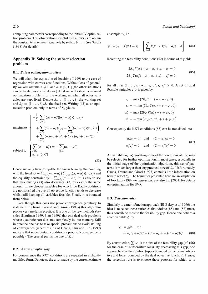
216 Smola and Scholkopf
computing parameters corresponding to the initial SV optimiza-tion problem. This observation is useful as it allows us to obtainthe constant term b directly, namely by setting b = y. (see Smola(1998) for details).
Appendix B: Solving the subset selectionproblem
B.1. Subset optimization problem
We will adapt the exposition of Joachims (1999) to the case ofregression with convex cost functions. Without loss of general-ity we will assume ε �= 0 and α ∈ [0, C] (the other situationscan be treated as a special case). First we will extract a reducedoptimization problem for the working set when all other vari-ables are kept fixed. Denote Sw ⊂ {1, . . . , �} the working setand S f := {1, . . . , �}\Sw the fixed set. Writing (43) as an opti-mization problem only in terms of Sw yields
maximize
−1
2
∑i, j∈Sw
(αi − α∗i )(α j − α∗
j )〈xi , x j 〉
+∑i∈Sw
(αi − α∗i )
(yi −
∑j∈S f
(α j − α∗j )〈xi , x j 〉
)
+∑i∈Sw
(−ε(αi + α∗i ) + C(T (αi ) + T (α∗
i )))
subject to
∑i∈Sw
(αi − α∗i ) = −
∑i∈S f
(αi − α∗i )
αi ∈ [0, C]
(83)
Hence we only have to update the linear term by the couplingwith the fixed set − ∑
i∈Sw(αi −α∗
i )∑
j∈S f(α j −α∗
j )〈xi , x j 〉 andthe equality constraint by − ∑
i∈S f(αi − α∗
i ). It is easy to seethat maximizing (83) also decreases (43) by exactly the sameamount. If we choose variables for which the KKT–conditionsare not satisfied the overall objective function tends to decreasewhilst still keeping all variables feasible. Finally it is boundedfrom below.
Even though this does not prove convergence (contrary tostatement in Osuna, Freund and Girosi (1997)) this algorithmproves very useful in practice. It is one of the few methods (be-sides (Kaufman 1999, Platt 1999)) that can deal with problemswhose quadratic part does not completely fit into memory. Stillin practice one has to take special precautions to avoid stallingof convergence (recent results of Chang, Hsu and Lin (1999)indicate that under certain conditions a proof of convergence ispossible). The crucial part is the one of Sw.
B.2. A note on optimality
For convenience the KKT conditions are repeated in a slightlymodified form. Denote ϕi the error made by the current estimate
at sample xi , i.e.
ϕi := yi − f (xi ) = yi −[
m∑j=1
k(xi , x j )(αi − α∗i ) + b
]. (84)
Rewriting the feasibility conditions (52) in terms of α yields
2∂αi T (αi ) + ε − ϕi + si − zi = 0(85)
2∂α∗iT (α∗
i ) + ε + ϕi + s∗i − z∗
i = 0
for all i ∈ {1, . . . , m} with zi , z∗i , si , s∗
i ≥ 0. A set of dualfeasible variables z, s is given by
zi = max(2∂αi T (αi ) + ε − ϕi , 0
)si = − min
(2∂αi T (αi ) + ε − ϕi , 0
)(86)
z∗i = max
(2∂α∗
iT (α∗
i ) + ε + ϕi , 0)
s∗i = − min
(2∂α∗
iT (α∗
i ) + ε + ϕi , 0)
Consequently the KKT conditions (53) can be translated into
αi zi = 0 and (C − αi )si = 0(87)
α∗i z∗
i = 0 and (C − α∗i )s∗
i = 0
All variables αi , α∗i violating some of the conditions of (87) may
be selected for further optimization. In most cases, especially inthe initial stage of the optimization algorithm, this set of pat-terns is much larger than any practical size of Sw. UnfortunatelyOsuna, Freund and Girosi (1997) contains little information onhow to select Sw. The heuristics presented here are an adaptationof Joachims (1999) to regression. See also Lin (2001) for detailson optimization for SVR.
B.3. Selection rules
Similarly to a merit function approach (El-Bakry et al. 1996) theidea is to select those variables that violate (85) and (87) most,thus contribute most to the feasibility gap. Hence one defines ascore variable ζi by
ζi := gi zi + si ti
= αi zi + α∗i z∗
i + (C − αi )si + (C − α∗i )s∗
i (88)
By construction,∑
i ζi is the size of the feasibility gap (cf. (56)for the case of ε-insensitive loss). By decreasing this gap, oneapproaches the the solution (upper bounded by the primal objec-tive and lower bounded by the dual objective function). Hence,the selection rule is to choose those patterns for which ζi is

A tutorial on support vector regression 217
largest. Some algorithms use
ζ ′i := αi�(zi ) + α∗
i �(z∗i )
+ (C − αi )�(si ) + (C − α∗i )�(si )
(89)or ζ ′′
i := �(αi )zi + �(α∗i )z∗
i
+ �(C − αi )si + �(C − α∗i )si .
One can see that ζi = 0, ζ ′i = 0, and ζ ′′
i = 0 mutually imply eachother. However, only ζi gives a measure for the contribution ofthe variable i to the size of the feasibility gap.
Finally, note that heuristics like assigning sticky–flags (cf.Burges 1998) to variables at the boundaries, thus effec-tively solving smaller subproblems, or completely removingthe corresponding patterns from the training set while ac-counting for their couplings (Joachims 1999) can signifi-cantly decrease the size of the problem one has to solve andthus result in a noticeable speedup. Also caching (Joachims1999, Kowalczyk 2000) of already computed entries of thedot product matrix may have a significant impact on theperformance.
Appendix C: Solving the SMO equations
C.1. Pattern dependent regularization
Consider the constrained optimization problem (83) for two in-dices, say (i, j). Pattern dependent regularization means that Ci
may be different for every pattern (possibly even different forαi and α∗
i ). Since at most two variables may become nonzeroat the same time and moreover we are dealing with a con-strained optimization problem we may express everything interms of just one variable. From the summation constraint weobtain
(αi − α∗i ) + (α j − α∗
j ) = (αold
i − α∗i
old) + (αold
j − α∗jold) := γ
(90)
for regression. Exploiting α(∗)j ∈ [0, C (∗)
j ] yields α(∗)i ∈ [L , H ].
This is taking account of the fact that there may be only fourdifferent pairs of nonzero variables: (αi , α j ), (α∗
i , α j ), (αi , α∗j ),
and (α∗i , α
∗j ). For convenience define an auxiliary variables s
such that s = 1 in the first and the last case and s = −1 other-wise.
α j α∗j
αi L max(0, γ − C j ) max(0, γ )H min(Ci , γ ) min(Ci , C∗
j + γ )α∗
i L max(0, −γ ) max(0, −γ − C∗j )
H min(C∗i , −γ + C j ) min(C∗
i , −γ )
C.2. Analytic solution for regression
Next one has to solve the optimization problem analytically. Wemake use of (84) and substitute the values of φi into the reducedoptimization problem (83). In particular we use
yi −∑j �∈Sw
(αi − α∗i )Ki j = ϕi + b +
∑j∈Sw
(αold
i − α∗i
old)Ki j .
(91)
Moreover with the auxiliary variables γ = αi −α∗i +α j −α∗
j andη := (Kii + K j j − 2Ki j ) one obtains the following constrainedoptimization problem in i (after eliminating j , ignoring termsindependent of α j , α
∗j and noting that this only holds for αiα
∗i =
α jα∗j = 0):
maximize − 1
2(αi − α∗
i )2η − ε(αi + α∗i )(1 − s)
+ (αi − α∗i )
(φi − φ j + η
(αold
i − α∗i
old)) (92)
subject to α(∗)i ∈ [L (∗), H (∗)].
The unconstrained maximum of (92) with respect to αi or α∗i
can be found below.
(I) αi , α j αoldi + η−1(ϕi − ϕ j )
(II) αi , α∗j αold
i + η−1(ϕi − ϕ j − 2ε)(III) α∗
i , α j α∗i
old − η−1(ϕi − ϕ j + 2ε)(IV) α∗
i , α∗j α∗
iold − η−1(ϕi − ϕ j )
The problem is that we do not know beforehand which of thefour quadrants (I)–(IV) contains the solution. However, by con-sidering the sign of γ we can distinguish two cases: for γ > 0only (I)–(III) are possible, for γ < 0 the coefficients satisfy oneof the cases (II)–(IV). In case of γ = 0 only (II) and (III) haveto be considered. See also the diagram below.
For γ > 0 it is best to start with quadrant (I), test whether theunconstrained solution hits one of the boundaries L , H and if so,probe the corresponding adjacent quadrant (II) or (III). γ < 0can be dealt with analogously.
Due to numerical instabilities, it may happen that η < 0. Inthat case η should be set to 0 and one has to solve (92) in a linearfashion directly.11

218 Smola and Scholkopf
C.3. Selection rule for regression
Finally, one has to pick indices (i, j) such that the objectivefunction is maximized. Again, the reasoning of SMO (Platt 1999,Section 12.2.2) for classification will be mimicked. This meansthat a two loop approach is chosen to maximize the objectivefunction. The outer loop iterates over all patterns violating theKKT conditions, first only over those with Lagrange multipliersneither on the upper nor lower boundary, and once all of themare satisfied, over all patterns violating the KKT conditions, toensure self consistency on the complete dataset.12 This solvesthe problem of choosing i .
Now for j : To make a large step towards the minimum, onelooks for large steps in αi . As it is computationally expensive tocompute η for all possible pairs (i, j) one chooses the heuristic tomaximize the absolute value of the numerator in the expressionsfor αi and α∗
i , i.e. |ϕi − ϕ j | and |ϕi − ϕ j ± 2ε|. The index jcorresponding to the maximum absolute value is chosen for thispurpose.
If this heuristic happens to fail, in other words if little progressis made by this choice, all other indices j are looked at (this iswhat is called “second choice hierarcy” in Platt (1999) in thefollowing way:
1. All indices j corresponding to non–bound examples arelooked at, searching for an example to make progress on.
2. In the case that the first heuristic was unsuccessful, allother samples are analyzed until an example is found whereprogress can be made.
3. If both previous steps fail proceed to the next i .
For a more detailed discussion (see Platt 1999). Unlike interiorpoint algorithms SMO does not automatically provide a valuefor b. However this can be chosen like in Section 1.4 by havinga close look at the Lagrange multipliers α
(∗)i obtained.
C.4. Stopping criteria
By essentially minimizing a constrained primal optimizationproblem one cannot ensure that the dual objective function in-creases with every iteration step.13 Nevertheless one knows thatthe minimum value of the objective function lies in the interval[dual objectivei , primal objectivei ] for all steps i , hence also inthe interval [(max j≤i dual objective j ), primal objectivei ]. Oneuses the latter to determine the quality of the current solution.
The calculation of the primal objective function from the pre-diction errors is straightforward. One uses
∑i, j
(αi − α∗i )(α j − α∗
j )ki j = −∑
i
(αi − α∗i )(ϕi + yi − b),
(93)
i.e. the definition of ϕi to avoid the matrix–vector multiplicationwith the dot product matrix.
Acknowledgments
This work has been supported in part by a grant of the DFG(Ja 379/71, Sm 62/1). The authors thank Peter Bartlett, ChrisBurges, Stefan Harmeling, Olvi Mangasarian, Klaus-RobertMuller, Vladimir Vapnik, Jason Weston, Robert Williamson, andAndreas Ziehe for helpful discussions and comments.
Notes
1. Our use of the term ‘regression’ is somewhat lose in that it also includescases of function estimation where one minimizes errors other than the meansquare loss. This is done mainly for historical reasons (Vapnik, Golowichand Smola 1997).
2. A similar approach, however using linear instead of quadratic programming,was taken at the same time in the USA, mainly by Mangasarian (1965, 1968,1969).
3. See Smola (1998) for an overview over other ways of specifying flatness ofsuch functions.
4. This is true as long as the dimensionality of w is much higher than thenumber of observations. If this is not the case, specialized methods canoffer considerable computational savings (Lee and Mangasarian 2001).
5. The table displays CT(α) instead of T (α) since the former can be pluggeddirectly into the corresponding optimization equations.
6. The high price tag usually is the major deterrent for not using them. Moreoverone has to bear in mind that in SV regression, one may speed up the solutionconsiderably by exploiting the fact that the quadratic form has a specialstructure or that there may exist rank degeneracies in the kernel matrixitself.
7. For large and noisy problems (e.g. 100.000 patterns and more with a substan-tial fraction of nonbound Lagrange multipliers) it is impossible to solve theproblem exactly: due to the size one has to use subset selection algorithms,hence joint optimization over the training set is impossible. However, unlikein Neural Networks, we can determine the closeness to the optimum. Notethat this reasoning only holds for convex cost functions.
8. A similar technique was employed by Bradley and Mangasarian (1998) inthe context of linear programming in order to deal with large datasets.
9. Due to length constraints we will not deal with the connection betweenGaussian Processes and SVMs. See Williams (1998) for an excellentoverview.
10. Strictly speaking, in Bayesian estimation one is not so much concerned aboutthe maximizer ˆf of p( f | X ) but rather about the posterior distribution off .
11. Negative values of η are theoretically impossible since k satisfies Mercer’scondition: 0 ≤ ‖�(xi ) − �(x j )‖2 = Kii + K j j − 2Ki j = η.
12. It is sometimes useful, especially when dealing with noisy data, to iterateover the complete KKT violating dataset already before complete self con-sistency on the subset has been achieved. Otherwise much computationalresources are spent on making subsets self consistent that are not globallyself consistent. This is the reason why in the pseudo code a global loopis initiated already when only less than 10% of the non bound variableschanged.
13. It is still an open question how a subset selection optimization algorithmcould be devised that decreases both primal and dual objective functionat the same time. The problem is that this usually involves a number ofdual variables of the order of the sample size, which makes this attemptunpractical.
References
Aizerman M.A., Braverman E.M., and Rozonoer L.I. 1964. Theoreticalfoundations of the potential function method in pattern recognitionlearning. Automation and Remote Control 25: 821–837.
Aronszajn N. 1950. Theory of reproducing kernels. Transactions of theAmerican Mathematical Society 68: 337–404.

A tutorial on support vector regression 219
Bazaraa M.S., Sherali H.D., and Shetty C.M. 1993. Nonlinear Program-ming: Theory and Algorithms, 2nd edition, Wiley.
Bellman R.E. 1961. Adaptive Control Processes. Princeton UniversityPress, Princeton, NJ.
Bennett K. 1999. Combining support vector and mathematical program-ming methods for induction. In: Scholkopf B., Burges C.J.C., andSmola A.J., (Eds.), Advances in Kernel Methods—SV Learning,MIT Press, Cambridge, MA, pp. 307–326.
Bennett K.P. and Mangasarian O.L. 1992. Robust linear program-ming discrimination of two linearly inseparable sets. OptimizationMethods and Software 1: 23–34.
Berg C., Christensen J.P.R., and Ressel P. 1984. Harmonic Analysis onSemigroups. Springer, New York.
Bertsekas D.P. 1995. Nonlinear Programming. Athena Scientific,Belmont, MA.
Bishop C.M. 1995. Neural Networks for Pattern Recognition.Clarendon Press, Oxford.
Blanz V., Scholkopf B., Bulthoff H., Burges C., Vapnik V., and VetterT. 1996. Comparison of view-based object recognition algorithmsusing realistic 3D models. In: von der Malsburg C., von SeelenW., Vorbruggen J.C., and Sendhoff B. (Eds.), Artificial NeuralNetworks ICANN’96, Berlin. Springer Lecture Notes in ComputerScience, Vol. 1112, pp. 251–256.
Bochner S. 1959. Lectures on Fourier integral. Princeton Univ. Press,Princeton, New Jersey.
Boser B.E., Guyon I.M., and Vapnik V.N. 1992. A training algorithm foroptimal margin classifiers. In: Haussler D. (Ed.), Proceedings ofthe Annual Conference on Computational Learning Theory. ACMPress, Pittsburgh, PA, pp. 144–152.
Bradley P.S., Fayyad U.M., and Mangasarian O.L. 1998. Data min-ing: Overview and optimization opportunities. Technical Re-port 98–01, University of Wisconsin, Computer Sciences Depart-ment, Madison, January. INFORMS Journal on Computing, toappear.
Bradley P.S. and Mangasarian O.L. 1998. Feature selection via con-cave minimization and support vector machines. In: Shavlik J.(Ed.), Proceedings of the International Conference on MachineLearning, Morgan Kaufmann Publishers, San Francisco, Califor-nia, pp. 82–90. ftp://ftp.cs.wisc.edu/math-prog/tech-reports/98-03.ps.Z.
Bunch J.R. and Kaufman L. 1977. Some stable methods for calculat-ing inertia and solving symmetric linear systems. Mathematics ofComputation 31: 163–179.
Bunch J.R. and Kaufman L. 1980. A computational method for theindefinite quadratic programming problem. Linear Algebra andIts Applications, pp. 341–370, December.
Bunch J.R., Kaufman L., and Parlett B. 1976. Decomposition of a sym-metric matrix. Numerische Mathematik 27: 95–109.
Burges C.J.C. 1996. Simplified support vector decision rules. InL. Saitta (Ed.), Proceedings of the International Conference onMachine Learning, Morgan Kaufmann Publishers, San Mateo,CA, pp. 71–77.
Burges C.J.C. 1998. A tutorial on support vector machines for patternrecognition. Data Mining and Knowledge Discovery 2(2): 121–167.
Burges C.J.C. 1999. Geometry and invariance in kernel based methods.In Scholkopf B., Burges C.J.C., and Smola A.J., (Eds.), Advancesin Kernel Methods—Support Vector Learning, MIT Press, Cam-bridge, MA, pp. 89–116.
Burges C.J.C. and Scholkopf B. 1997. Improving the accuracy and speedof support vector learning machines. In Mozer M.C., Jordan M.I.,and Petsche T., (Eds.), Advances in Neural Information ProcessingSystems 9, MIT Press, Cambridge, MA, pp. 375–381.
Chalimourda A., Scholkopf B., and Smola A.J. 2004. Experimentallyoptimal ν in support vector regression for different noise modelsand parameter settings. Neural Networks 17(1): 127–141.
Chang C.-C., Hsu C.-W., and Lin C.-J. 1999. The analysis of decom-position methods for support vector machines. In Proceeding ofIJCAI99, SVM Workshop.
Chang C.C. and Lin C.J. 2001. Training ν-support vector classi-fiers: Theory and algorithms. Neural Computation 13(9): 2119–2147.
Chen S., Donoho D., and Saunders M. 1999. Atomic decomposition bybasis pursuit. Siam Journal of Scientific Computing 20(1): 33–61.
Cherkassky V. and Mulier F. 1998. Learning from Data. John Wiley andSons, New York.
Cortes C. and Vapnik V. 1995. Support vector networks. Machine Learn-ing 20: 273–297.
Cox D. and O’Sullivan F. 1990. Asymptotic analysis of penalized like-lihood and related estimators. Annals of Statistics 18: 1676–1695.
CPLEX Optimization Inc. Using the CPLEX callable library. Manual,1994.
Cristianini N. and Shawe-Taylor J. 2000. An Introduction to SupportVector Machines. Cambridge University Press, Cambridge, UK.
Cristianini N., Campbell C., and Shawe-Taylor J. 1998. Multiplicativeupdatings for support vector learning. NeuroCOLT Technical Re-port NC-TR-98-016, Royal Holloway College.
Dantzig G.B. 1962. Linear Programming and Extensions. PrincetonUniv. Press, Princeton, NJ.
Devroye L., Gyorfi L., and Lugosi G. 1996. A Probabilistic Theory ofPattern Recognition. Number 31 in Applications of mathematics.Springer, New York.
Drucker H., Burges C.J.C., Kaufman L., Smola A., and Vapnik V. 1997.Support vector regression machines. In: Mozer M.C., Jordan M.I.,and Petsche T. (Eds.), Advances in Neural Information ProcessingSystems 9, MIT Press, Cambridge, MA, pp. 155–161.
Efron B. 1982. The jacknife, the bootstrap, and other resampling plans.SIAM, Philadelphia.
Efron B. and Tibshirani R.J. 1994. An Introduction to the Bootstrap.Chapman and Hall, New York.
El-Bakry A., Tapia R., Tsuchiya R., and Zhang Y. 1996. On the formula-tion and theory of the Newton interior-point method for nonlinearprogramming. J. Optimization Theory and Applications 89: 507–541.
Fletcher R. 1989. Practical Methods of Optimization. John Wiley andSons, New York.
Girosi F. 1998. An equivalence between sparse approximation and sup-port vector machines. Neural Computation 10(6): 1455–1480.
Girosi F., Jones M., and Poggio T. 1993. Priors, stabilizers and ba-sis functions: From regularization to radial, tensor and additivesplines. A.I. Memo No. 1430, Artificial Intelligence Laboratory,Massachusetts Institute of Technology.
Guyon I., Boser B., and Vapnik V. 1993. Automatic capacity tuning ofvery large VC-dimension classifiers. In: Hanson S.J., Cowan J.D.,and Giles C.L. (Eds.), Advances in Neural Information ProcessingSystems 5. Morgan Kaufmann Publishers, pp. 147–155.
Hardle W. 1990. Applied nonparametric regression, volume 19 ofEconometric Society Monographs. Cambridge University Press.

220 Smola and Scholkopf
Hastie T.J. and Tibshirani R.J. 1990. Generalized Additive Models,volume 43 of Monographs on Statistics and Applied Probability.Chapman and Hall, London.
Haykin S. 1998. Neural Networks: A Comprehensive Foundation. 2ndedition. Macmillan, New York.
Hearst M.A., Scholkopf B., Dumais S., Osuna E., and Platt J. 1998.Trends and controversies—support vector machines. IEEE Intel-ligent Systems 13: 18–28.
Herbrich R. 2002. Learning Kernel Classifiers: Theory and Algorithms.MIT Press.
Huber P.J. 1972. Robust statistics: A review. Annals of Statistics43: 1041.
Huber P.J. 1981. Robust Statistics. John Wiley and Sons, New York.IBM Corporation. 1992. IBM optimization subroutine library guide
and reference. IBM Systems Journal, 31, SC23-0519.Jaakkola T.S. and Haussler D. 1999. Probabilistic kernel regression
models. In: Proceedings of the 1999 Conference on AI and Statis-tics.
Joachims T. 1999. Making large-scale SVM learning practical.In: Scholkopf B., Burges C.J.C., and Smola A.J. (Eds.), Ad-vances in Kernel Methods—Support Vector Learning, MIT Press,Cambridge, MA, pp. 169–184.
Karush W. 1939. Minima of functions of several variables with inequal-ities as side constraints. Master’s thesis, Dept. of Mathematics,Univ. of Chicago.
Kaufman L. 1999. Solving the quadratic programming problem arisingin support vector classification. In: Scholkopf B., Burges C.J.C.,and Smola A.J. (Eds.), Advances in Kernel Methods—SupportVector Learning, MIT Press, Cambridge, MA, pp. 147–168
Keerthi S.S., Shevade S.K., Bhattacharyya C., and Murthy K.R.K. 1999.Improvements to Platt’s SMO algorithm for SVM classifier design.Technical Report CD-99-14, Dept. of Mechanical and ProductionEngineering, Natl. Univ. Singapore, Singapore.
Keerthi S.S., Shevade S.K., Bhattacharyya C., and Murty K.R.K. 2001.Improvements to platt’s SMO algorithm for SVM classifier design.Neural Computation 13: 637–649.
Kimeldorf G.S. and Wahba G. 1970. A correspondence betweenBayesian estimation on stochastic processes and smoothing bysplines. Annals of Mathematical Statistics 41: 495–502.
Kimeldorf G.S. and Wahba G. 1971. Some results on Tchebycheffianspline functions. J. Math. Anal. Applic. 33: 82–95.
Kowalczyk A. 2000. Maximal margin perceptron. In: Smola A.J.,Bartlett P.L., Scholkopf B., and Schuurmans D. (Eds.), Advancesin Large Margin Classifiers, MIT Press, Cambridge, MA, pp. 75–113.
Kuhn H.W. and Tucker A.W. 1951. Nonlinear programming. In: Proc.2nd Berkeley Symposium on Mathematical Statistics and Proba-bilistics, Berkeley. University of California Press, pp. 481–492.
Lee Y.J. and Mangasarian O.L. 2001. SSVM: A smooth support vectormachine for classification. Computational optimization and Ap-plications 20(1): 5–22.
Li M. and Vitanyi P. 1993. An introduction to Kolmogorov Complexityand its applications. Texts and Monographs in Computer Science.Springer, New York.
Lin C.J. 2001. On the convergence of the decomposition method forsupport vector machines. IEEE Transactions on Neural Networks12(6): 1288–1298.
Lustig I.J., Marsten R.E., and Shanno D.F. 1990. On implementingMehrotra’s predictor-corrector interior point method for linear pro-
gramming. Princeton Technical Report SOR 90–03., Dept. of CivilEngineering and Operations Research, Princeton University.
Lustig I.J., Marsten R.E., and Shanno D.F. 1992. On implement-ing Mehrotra’s predictor-corrector interior point method for lin-ear programming. SIAM Journal on Optimization 2(3): 435–449.
MacKay D.J.C. 1991. Bayesian Methods for Adaptive Models. PhDthesis, Computation and Neural Systems, California Institute ofTechnology, Pasadena, CA.
Mangasarian O.L. 1965. Linear and nonlinear separation of patterns bylinear programming. Operations Research 13: 444–452.
Mangasarian O.L. 1968. Multi-surface method of pattern separation.IEEE Transactions on Information Theory IT-14: 801–807.
Mangasarian O.L. 1969. Nonlinear Programming. McGraw-Hill, NewYork.
Mattera D. and Haykin S. 1999. Support vector machines for dy-namic reconstruction of a chaotic system. In: Scholkopf B., BurgesC.J.C., and Smola A.J. (Eds.), Advances in Kernel Methods—Support Vector Learning, MIT Press, Cambridge, MA, pp. 211–242.
McCormick G.P. 1983. Nonlinear Programming: Theory, Algorithms,and Applications. John Wiley and Sons, New York.
Megiddo N. 1989. Progressin Mathematical Programming, chapterPathways to the optimal set in linear programming, Springer, NewYork, NY, pp. 131–158.
Mehrotra S. and Sun J. 1992. On the implementation of a (primal-dual)interior point method. SIAM Journal on Optimization 2(4): 575–601.
Mercer J. 1909. Functions of positive and negative type and their con-nection with the theory of integral equations. Philosophical Trans-actions of the Royal Society, London A 209: 415–446.
Micchelli C.A. 1986. Algebraic aspects of interpolation. Proceedingsof Symposia in Applied Mathematics 36: 81–102.
Morozov V.A. 1984. Methods for Solving Incorrectly Posed Problems.Springer.
Muller K.-R., Smola A., Ratsch G., Scholkopf B., Kohlmorgen J., andVapnik V. 1997. Predicting time series with support vector ma-chines. In: Gerstner W., Germond A., Hasler M., and Nicoud J.-D.(Eds.), Artificial Neural Networks ICANN’97, Berlin. SpringerLecture Notes in Computer Science Vol. 1327 pp. 999–1004.
Murtagh B.A. and Saunders M.A. 1983. MINOS 5.1 user’s guide. Tech-nical Report SOL 83-20R, Stanford University, CA, USA, Revised1987.
Neal R. 1996. Bayesian Learning in Neural Networks. Springer.Nilsson N.J. 1965. Learning machines: Foundations of Trainable Pattern
Classifying Systems. McGraw-Hill.Nyquist. H. 1928. Certain topics in telegraph transmission theory.
Trans. A.I.E.E., pp. 617–644.Osuna E., Freund R., and Girosi F. 1997. An improved training algo-
rithm for support vector machines. In Principe J., Gile L., MorganN., and Wilson E. (Eds.), Neural Networks for Signal ProcessingVII—Proceedings of the 1997 IEEE Workshop, pp. 276–285, NewYork, IEEE.
Osuna E. and Girosi F. 1999. Reducing the run-time complexity insupport vector regression. In: Scholkopf B., Burges C.J.C., andSmola A. J. (Eds.), Advances in Kernel Methods—Support VectorLearning, pp. 271–284, Cambridge, MA, MIT Press.
Ovari Z. 2000. Kernels, eigenvalues and support vector machines. Hon-ours thesis, Australian National University, Canberra.

A tutorial on support vector regression 221
Platt J. 1999. Fast training of support vector machines using sequen-tial minimal optimization. In: Scholkopf B., Burges C.J.C., andSmola A.J. (Eds.) Advances in Kernel Methods—Support VectorLearning, pp. 185–208, Cambridge, MA, MIT Press.
Poggio T. 1975. On optimal nonlinear associative recall. BiologicalCybernetics, 19: 201–209.
Rasmussen C. 1996. Evaluation of Gaussian Processes andOther Methods for Non-Linear Regression. PhD thesis,Department of Computer Science, University of Toronto,ftp://ftp.cs.toronto.edu/pub/carl/thesis.ps.gz.
Rissanen J. 1978. Modeling by shortest data description. Automatica,14: 465–471.
Saitoh S. 1988. Theory of Reproducing Kernels and its Applications.Longman Scientific & Technical, Harlow, England.
Saunders C., Stitson M.O., Weston J., Bottou L., Scholkopf B., andSmola A. 1998. Support vector machine—reference manual. Tech-nical Report CSD-TR-98-03, Department of Computer Science,Royal Holloway, University of London, Egham, UK. SVM avail-able at http://svm.dcs.rhbnc.ac.uk/.
Schoenberg I. 1942. Positive definite functions on spheres. DukeMath. J., 9: 96–108.
Scholkopf B. 1997. Support Vector Learning. R. OldenbourgVerlag, Munchen. Doktorarbeit, TU Berlin. Download:http://www.kernel-machines.org.
Scholkopf B., Burges C., and Vapnik V. 1995. Extracting support datafor a given task. In: Fayyad U.M. and Uthurusamy R. (Eds.), Pro-ceedings, First International Conference on Knowledge Discovery& Data Mining, Menlo Park, AAAI Press.
Scholkopf B., Burges C., and Vapnik V. 1996. Incorporating invariancesin support vector learning machines. In: von der Malsburg C., vonSeelen W., Vorbruggen J. C., and Sendhoff B. (Eds.), ArtificialNeural Networks ICANN’96, pp. 47–52, Berlin, Springer LectureNotes in Computer Science, Vol. 1112.
Scholkopf B., Burges C.J.C., and Smola A.J. 1999a. (Eds.) Ad-vances in Kernel Methods—Support Vector Learning. MIT Press,Cambridge, MA.
Scholkopf B., Herbrich R., Smola A.J., and Williamson R.C. 2001. Ageneralized representer theorem. Technical Report 2000-81, Neu-roCOLT, 2000. To appear in Proceedings of the Annual Conferenceon Learning Theory, Springer (2001).
Scholkopf B., Mika S., Burges C., Knirsch P., Muller K.-R., Ratsch G.,and Smola A. 1999b. Input space vs. feature space in kernel-basedmethods. IEEE Transactions on Neural Networks, 10(5): 1000–1017.
Scholkopf B., Platt J., Shawe-Taylor J., Smola A.J. , and Williamson R.C.2001. Estimating the support of a high-dimensional distribution.Neural Computation, 13(7): 1443–1471.
Scholkopf B., Simard P., Smola A., and Vapnik V. 1998a. Prior knowl-edge in support vector kernels. In: Jordan M.I., Kearns M.J., andSolla S.A. (Eds.) Advances in Neural Information Processing Sys-tems 10, MIT Press. Cambridge, MA, pp. 640–646.
Scholkopf B., Smola A., and Muller K.-R. 1998b. Nonlinear compo-nent analysis as a kernel eigenvalue problem. Neural Computation,10: 1299–1319.
Scholkopf B., Smola A., Williamson R.C., and Bartlett P.L. 2000. Newsupport vector algorithms. Neural Computation, 12: 1207–1245.
Scholkopf B. and Smola A.J. 2002. Learning with Kernels. MIT Press.Scholkopf B., Sung K., Burges C., Girosi F., Niyogi P., Poggio T.,
and Vapnik V. 1997. Comparing support vector machines with
Gaussian kernels to radial basis function classifiers. IEEE Trans-actions on Signal Processing, 45: 2758–2765.
Shannon C.E. 1948. A mathematical theory of communication. BellSystem Technical Journal, 27: 379–423, 623–656.
Shawe-Taylor J., Bartlett P.L., Williamson R.C., and Anthony M.1998. Structural risk minimization over data-dependent hierar-chies. IEEE Transactions on Information Theory, 44(5): 1926–1940.
Smola A., Murata N., Scholkopf B., and Muller K.-R. 1998a. Asymp-totically optimal choice of ε-loss for support vector machines.In: Niklasson L., Boden M., and Ziemke T. (Eds.) Proceed-ings of the International Conference on Artificial Neural Net-works, Perspectives in Neural Computing, pp. 105–110, Berlin,Springer.
Smola A., Scholkopf B., and Muller K.-R. 1998b. The connection be-tween regularization operators and support vector kernels. NeuralNetworks, 11: 637–649.
Smola A., Scholkopf B., and Muller K.-R. 1998c. General cost func-tions for support vector regression. In: Downs T., Frean M.,and Gallagher M. (Eds.) Proc. of the Ninth Australian Conf. onNeural Networks, pp. 79–83, Brisbane, Australia. University ofQueensland.
Smola A., Scholkopf B., and Ratsch G. 1999. Linear programs forautomatic accuracy control in regression. In: Ninth InternationalConference on Artificial Neural Networks, Conference Publica-tions No. 470, pp. 575–580, London. IEE.
Smola. A.J. 1996. Regression estimation with support vector learningmachines. Diplomarbeit, Technische Universitat Munchen.
Smola A.J. 1998. Learning with Kernels. PhD thesis, Technische Uni-versitat Berlin. GMD Research Series No. 25.
Smola A.J., Elisseeff A., Scholkopf B., and Williamson R.C. 2000.Entropy numbers for convex combinations and MLPs. In SmolaA.J., Bartlett P.L., Scholkopf B., and Schuurmans D. (Eds.) Ad-vances in Large Margin Classifiers, MIT Press, Cambridge, MA,pp. 369–387.
Smola A.J., Ovari Z.L., and Williamson R.C. 2001. Regularization withdot-product kernels. In: Leen T.K., Dietterich T.G., and Tresp V.(Eds.) Advances in Neural Information Processing Systems 13,MIT Press, pp. 308–314.
Smola A.J. and Scholkopf B. 1998a. On a kernel-based method forpattern recognition, regression, approximation and operator in-version. Algorithmica, 22: 211–231.
Smola A.J. and Scholkopf B. 1998b. A tutorial on support vector re-gression. NeuroCOLT Technical Report NC-TR-98-030, RoyalHolloway College, University of London, UK.
Smola A.J. and Scholkopf B. 2000. Sparse greedy matrix approximationfor machine learning. In: Langley P. (Ed.), Proceedings of the In-ternational Conference on Machine Learning, Morgan KaufmannPublishers, San Francisco, pp. 911–918.
Stitson M., Gammerman A., Vapnik V., Vovk V., Watkins C., andWeston J. 1999. Support vector regression with ANOVA decom-position kernels. In: Scholkopf B., Burges C.J.C., and Smola A.J.(Eds.), Advances in Kernel Methods—Support Vector Learning,MIT Press Cambridge, MA, pp. 285–292.
Stone C.J. 1985. Additive regression and other nonparametric models.Annals of Statistics, 13: 689–705.
Stone M. 1974. Cross-validatory choice and assessment of statisticalpredictors (with discussion). Journal of the Royal Statistical Soci-ety, B36: 111–147.

222 Smola and Scholkopf
Street W.N. and Mangasarian O.L. 1995. Improved generalization viatolerant training. Technical Report MP-TR-95-11, University ofWisconsin, Madison.
Tikhonov A.N. and Arsenin V.Y. 1977. Solution of Ill-posed problems.V. H. Winston and Sons.
Tipping M.E. 2000. The relevance vector machine. In: Solla S.A., LeenT.K., and Muller K.-R. (Eds.), Advances in Neural InformationProcessing Systems 12, MIT Press, Cambridge, MA, pp. 652–658.
Vanderbei R.J. 1994. LOQO: An interior point code for quadratic pro-gramming. TR SOR-94-15, Statistics and Operations Research,Princeton Univ., NJ.
Vanderbei R.J. 1997. LOQO user’s manual—version 3.10. TechnicalReport SOR-97-08, Princeton University, Statistics and Oper-ations Research, Code available at http://www.princeton.edu/˜rvdb/.
Vapnik V. 1995. The Nature of Statistical Learning Theory. Springer,New York.
Vapnik V. 1998. Statistical Learning Theory. John Wiley and Sons,New York.
Vapnik. V. 1999. Three remarks on the support vector method offunction estimation. In: Scholkopf B., Burges C.J.C., and SmolaA.J. (Eds.), Advances in Kernel Methods—Support VectorLearning, MIT Press, Cambridge, MA, pp. 25–42.
Vapnik V. and Chervonenkis A. 1964. A note on one class ofperceptrons. Automation and Remote Control, 25.
Vapnik V. and Chervonenkis A. 1974. Theory of Pattern Recognition[in Russian]. Nauka, Moscow. (German Translation: WapnikW. & Tscherwonenkis A., Theorie der Zeichenerkennung,Akademie-Verlag, Berlin, 1979).
Vapnik V., Golowich S., and Smola A. 1997. Support vector methodfor function approximation, regression estimation, and signalprocessing. In: Mozer M.C., Jordan M.I., and Petsche T. (Eds.)Advances in Neural Information Processing Systems 9, MA, MITPress, Cambridge. pp. 281–287.
Vapnik V. and Lerner A. 1963. Pattern recognition using generalizedportrait method. Automation and Remote Control, 24: 774–780.
Vapnik V.N. 1982. Estimation of Dependences Based on EmpiricalData. Springer, Berlin.
Vapnik V.N. and Chervonenkis A.Y. 1971. On the uniform convergenceof relative frequencies of events to their probabilities. Theory ofProbability and its Applications, 16(2): 264–281.
Wahba G. 1980. Spline bases, regularization, and generalizedcross-validation for solving approximation problems with largequantities of noisy data. In: Ward J. and Cheney E. (Eds.), Proceed-ings of the International Conference on Approximation theory inhonour of George Lorenz, Academic Press, Austin, TX, pp. 8–10.
Wahba G. 1990. Spline Models for Observational Data, volume 59 ofCBMS-NSF Regional Conference Series in Applied Mathematics.SIAM, Philadelphia.
Wahba G. 1999. Support vector machines, reproducing kernel Hilbertspaces and the randomized GACV. In: Scholkopf B., BurgesC.J.C., and Smola A.J. (Eds.), Advances in Kernel Methods—Support Vector Learning, MIT Press, Cambridge, MA. pp. 69–88.
Weston J., Gammerman A., Stitson M., Vapnik V., Vovk V., and WatkinsC. 1999. Support vector density estimation. In: Scholkopf B.,Burges C.J.C., and Smola A.J. (Eds.) Advances in KernelMethods—Support Vector Learning, MIT Press, Cambridge,MA. pp. 293–306.
Williams C.K.I. 1998. Prediction with Gaussian processes: From linearregression to linear prediction and beyond. In: Jordan M.I. (Ed.),Learning and Inference in Graphical Models, Kluwer Academic,pp. 599–621.
Williamson R.C., Smola A.J., and Scholkopf B. 1998. Generalizationperformance of regularization networks and support vectormachines via entropy numbers of compact operators. TechnicalReport 19, NeuroCOLT, http://www.neurocolt.com. Publishedin IEEE Transactions on Information Theory, 47(6): 2516–2532(2001).
Yuille A. and Grzywacz N. 1988. The motion coherence theory.In: Proceedings of the International Conference on ComputerVision, IEEE Computer Society Press, Washington, DC, pp. 344–354.