A Tutorial on Programming in Feldspar

A Tutorial on Programming in Feldspar

Emil Axelsson Anders Persson Mary Sheeran Josef SvenningssonGergely Devai

April 27, 2011

Introduction

Feldspar is a Domain Specific Language for programming DSP algorithms. It is implemented as am embeddedlanguage in the functional programming language Haskell. To find out more about our motivations in design-ing and implementing Feldspar, please see our paper from MemoCode 2010 (http://www.cse.chalmers.se/~ms/MemoCode.pdf) or our paper from the post-conference proceedings for IFL 2010 (http://www.cse.chalmers.se/

~ms/IFL_post_final.pdf). This document is not an exhaustive description of Feldspar, but a tutorial designedto get you started using the language. The Haddock documentation of Feldspar (http://hackage.haskell.org/package/feldspar-language) provides information about individual functions. Readers familiar with Haskell mayalso find it useful to browse the Feldspar source code – for example that implmenting the Vector and Stream librariesdescribed below.

A file containing many of the examples described in this tutorial is located at Examples/Tutorial/Tutorial.hs,bundled with the package (http://hackage.haskell.org/package/feldspar-language).

A design decision in Feldspar was to make programming in Feldspar as much like programming in Haskell as possible.Feldspar is built around a core language, which is a purely functional language operating at about the same level ofabstraction as C. On top of this core, a number of libraries are built, to enable programming at a higher level. Wewill return to some of those libraries shortly. It is also possible for the user to program directly using core languageconsructs. This gives fine control over the resulting C code when it is needed. It also allows the user to build herown abstractions or libraries on top of the core. Many operations are always done at the core level, simply becausethey do not need to be more abstract. This includes primitive functions like +, * or max.

Programs in the core language have the type Data a, where a is the type of the value computed by the program.Primitive functions in Feldspar work in the same way as their corresponding Haskell functions, except that theconstructor Data is added to all types. For example, the Haskell functions

(&&) :: Bool -> Bool -> Bool

(==) :: Eq a => a -> a -> Bool

(+) :: Num a => a -> a -> a

max :: Ord a => a -> a -> a

are reproduced as the following Feldspar functions:

(&&) :: Data Bool -> Data Bool -> Data Bool

(==) :: Eq a => Data a -> Data a -> Data Bool

(+) :: Numeric a => Data a -> Data a -> Data a

max :: Ord a => Data a -> Data a -> Data a

We can define simple Feldspar functions using Haskell’s function abstraction. For example:

1

http://www.cse.chalmers.se/~ms/MemoCode.pdf

http://www.cse.chalmers.se/~ms/MemoCode.pdf

http://www.cse.chalmers.se/~ms/IFL_post_final.pdf

http://www.cse.chalmers.se/~ms/IFL_post_final.pdf

http://hackage.haskell.org/package/feldspar-language



func :: Data Int32 -> Data Int32 -> Data Int32 -> Data Bool

func a b c = a + b == c

This program does not have a type of the form Data a, so it is not a simple core program. Think of it rather as aHaskell macro that builds a program from three smaller programs.

The function eval can be used to evaluate Feldspar functions. For example:

*Tutorial> eval (func 3 4 5)

False

Functions can only be evaluated in this way if provided with all of their inputs.

The icompile function is used to produce C code:

*Tutorial> icompile func

#include "feldspar_c99.h"

#include "feldspar_array.h"

#include <stdint.h>

#include <string.h>

#include <math.h>

#include <complex.h>

void test(struct array mem, int32_t in0, int32_t in1, int32_t in2, int * out3)

{

(* out3) = ((in0 + in1) == in2);

}

The first parameter of the resulting C function is not used here, and we will return to its use later. The remainingparameters correspond directly to the inputs and the output of the Feldspar function.

It is also possible to provide some arguments to the function at code generation time.

*Tutorial> icompile (func 3)



#include <stdint.h>

#include <string.h>

#include <math.h>


void test(struct array mem, int32_t in0, int32_t in1, int * out2)

{

(* out2) = ((3 + in0) == in1);

}

In addition to primitive types such as those that we have used so far, the core language also supports multidimen-sional arrays. Type-wise, an array is treated as a nested vector. For example, a two-dimensional array is thoughtof as a vector of rows, and each row is itself a vector of elements. Each level of an array has a type of the form [a],the same syntax as for Haskell lists where a is the type of the elements. Nesting is obtained by replacing a withanother array. For example, a three-dimensional array of integers has the type [[[ Int ]]]. An array representsa statically allocated block of memory in the final C code.

The function value converts a Haskell value into a Feldspar value. When given a Haskell list, it produces a corearray:

2

*Tutorial> eval (value [1..4 :: Int32])

[1,2,3,4]

It is useful to be able to ask for the type of an expression at the GHCi prompt using :t:

v1 = value [[1,2],[3,4],[5,(6::Int32)]]

*Tutorial> eval v1

[[1,2],[3,4],[5,6]]

*Tutorial> :t v1

v1 :: Data [[Int32]]

*Tutorial> eval (v1 ! 2)

[5,6]

The core language also includes a construct called parallel for computing the elements of a core array in a dataparallel manner.

parallel :: (Type a) => Data Length -> (Data Index -> Data a) -> Data [a]

The first argument is the number of elements to compute – the size. The second argument is a function mappingeach index (starting from 0) to its value. For example, the sequence [50,48, ... 2] can be computed by the followingprogram:

testParallel :: Data [Index]

testParallel = parallel 25 (\i -> 50-(2 * i))

Note that since each element of a parallel array can be computed independently from the others, the compiler isfree to generate code to compute them in any order it likes, even in parallel, if possible. (Note, however, that thecurrent compiler produces sequential C code.)

The core language contains a number of other constructs, including if-then-else and a for-loop. However, we willnot discuss these now, because the main point that we want to make is that Feldspar programmers should, wherepossible, program in terms of abstractions built from the core constructs. These abstractions are captured asseparate libraries. Think of these libraries as defining how to translate the abstractions being defined into the core;indeed the backend compiler only knows about the core. This separation has simplifed our implementation andmade it easier to play with different programming styles and abstractions. We stress that this experimentation isstill going on, and that we welcome input from potential users of Feldspar.

Vector library

Feldspar has a number of libraries that help the user to program at a high level of abstraction. Perhaps the mostimportant of these is the vector library. The central concept in this library is the Vector type. The main differencebetween vectors and arrays is that vectors are, in a sense, virtual. Vectors do no allocate any space in generated Cprograms unless the programmer explicitly forces allocation. This means that functions on vectors can be composedfreely and modularly and still result in efficient implementations. We will demonstrate this through examples.

Costless Abstraction

On of the most important features of the vector library is that it provides an optimization known as fusion. Fusion forvectors guarantees that all intermediate vectors in a program will be eliminated. This has the effect that operationson vectors can be written in a compositional style using many small functions that are composed together.

3

Let’s see an example of this. Suppose we wish to write a function that computes the scalar product of two vectors(also known as the dot product). Recall that the scalar product multiplies two vectors pointwise and then sums upthe resulting vector to produce a scalar. One way to code this up is to write it using a for-loop much like it wouldhave been written in C.

scalarProduct a b = forLoop (min (length a) (length b)) 0 (\ix sum -> sum + a!ix * b!ix)

If we set the lengths of the two input vectors to be 256 (and we will see later how to do this) and the types of theirelements to be integer, then the following C code is generated:

*Tutorial> sc



#include <stdint.h>

#include <string.h>

#include <math.h>


void test(struct array mem, struct array in0, struct array in1, int32_t * out2)

{

int32_t temp3;

(* out2) = 0;

{

uint32_t i4;

for(i4 = 0; i4 < 256; i4 += 1)

{

temp3 = ((* out2) + (at(int32_t,in0,i4) * at(int32_t,in1,i4)));

(* out2) = temp3;

}

}

}

The first parameter to the C function is not used in this example. We will return to this parameter and its uselater. The remaining parameters correspond to the two inputs and the output of the Feldspar function. The vectorinputs have been represented by structs of the following form:

struct array

{

void* buffer; /* pointer to the buffer of elements */

unsigned int length; /* number of elements in the array */

int elemSize; /* size of elements in bytes; (-1) for nested arrays */

};

and the at macro indexes into the actual buffer.

While it certainly works to write low level programs using the core language of Feldspar, it doesn’t really takeadvantage of the abstractions and optimizations that are provided. For-loops in the style of the Feldspar programabove can be rather opaque and difficult to understand, not to mention error-prone to write. The algorithm is alsonot very close to the description in prose of the scalar product.

The following scalar product function in Feldspar is clearer and more compositional:

scalarProduct as bs = sum (zipWith (*) as bs)

4

The function zipWith (*) takes care of pointwise multiplication, while the final summing is performed by the sum

function. The Feldspar program is now much closer to a mathematical description of the algorithm. Furthermore,if we keep the same sizes and types of the inputs, the generated C code is identical to the C code generated fromthe for-loop based version above. Our new scalar product function is much clearer and one might then expect thedownside to be generated code with lower performance. In this case, one might have expected to get two loops, onefor the zipWith and one for the summation. But that doesn’t happen because fusion eliminates the intermediatedata structure. It is this marriage of clear elegant programs with generated code of reasonable quality that Feldsparaims to achieve. In the following sections, we will explore the advantages and limitations of this approach to C codegeneration.

Programming with vectors

Vectors are represented by a length and an indexing function, and indices start at zero. The function indexed

builds a vector from a length and an index function. For example:

countUp :: Data Length -> DVector Index

countUp n = indexed n id

Here, the indexing function is actually the identity function (written id). This means that the value at index i ofthe vector will be i itself.

Having created a vector containing zero, one and so on, we can incremement each element of the vector as follows:

countUp1 :: Data Length -> DVector Index

countUp1 n = map (+1) (countUp n)

The function map f applies f to each element of a vector (just like the Haskell map on lists).

The function can be generalised to increment by m, and the incrementing can happen either in a map as in theprevious example, or in the indexing function itself:

countUpFrom :: Data Index -> Data Length -> DVector Index

countUpFrom m n = indexed n (+m)

To check out definitions like these, the user can call the eval function at the GHCi prompt, or name that call inher file and then type the shorter name at the prompt:

ex1 = eval (countUp1 6)

*Tutorial> ex1

[1,2,3,4,5,6]

Subsequences of the integers can also be constructed using the (...) operator, so that (1...6) gives the samevector as countUp1 6.

Many Haskell list processing functions are borrowed in Feldspar, and then work on vectors. For instance, thefunction reverse reverses a vector:

countDown :: Data Length -> DVector Index

countDown n = reverse (countUp n)

ex2 = eval (countDown 6)

*Tutorial> ex2

[5,4,3,2,1,0]

5

Now, let us move on to functions that take a vector as input. For example, we could define a function that reversesa vector and then increments each element by one either as

revmap0 :: DVector Float -> DVector Float

revmap0 xs = map (+1) (reverse xs)

or, equivalently, in point-free form, as

revmap :: DVector Float -> DVector Float

revmap = map (+1) . reverse

In the latter definition, we express how the function is built up from smaller components, while in the former wesay more explicitly what happens to the input data, which is named xs. Function composition is written as a dot(.) and happens from right to left. So, in revmap, the input vector is first reversed and then each of its elements isincremented by one. (In this case, the result is the same whatever order is chosen for the two operations, but thatis not always the case.)

We might also prefer to give the function a more general type.

revmap1 :: (Numeric a) => DVector a -> DVector a

revmap1 = map (+1) . reverse

The type a has to be one that supports numerical operations, and the constraint (Numeric a) must be included.Omitting such contraints leads to a type error, usually with a suggestion about what to add:

Examples\Tutorial\Tutorial.hs:134:16:

Could not deduce (Numeric a) from the context ()

arising from the literal ‘1’

at Examples\Tutorial\Tutorial.hs:134:16

Possible fix:

add (Numeric a) to the context of the type signature for ‘revmap1’

In the second argument of ‘(+)’, namely ‘1’

In the first argument of ‘map’, namely ‘(+ 1)’

In the first argument of ‘(.)’, namely ‘map (+ 1)’

We can test revmap1 by supplying it with an appropriate vector:

ex3 = eval (revmap1 (vector [0..5] :: DVector DefaultInt))

*Tutorial> ex3

[6,5,4,3,2,1]

The function vector takes a Haskell list as input, in this case the list [0..5]. Note how the type of the vector wasindicated. If this is not done, we get an error message:

Examples\Tutorial\Tutorial.hs:136:13:

Ambiguous type variable ‘t’ in the constraints:

‘Numeric t’

arising from a use of ‘revmap1’

at Examples\Tutorial\Tutorial.hs:136:13-35

‘Enum t’

arising from the arithmetic sequence ‘0 .. 5’

at Examples\Tutorial\Tutorial.hs:136:29-34

Possible cause: the monomorphism restriction applied to the following:

6

ex3’ :: Internal (DVector t)

(bound at Examples\Tutorial\Tutorial.hs:136:0)

Probable fix: give these definition(s) an explicit type signature

or use -XNoMonomorphismRestriction

DVector a is shorthand for Vector (Data a). Some further shorthands can easily be defined if the user dislikeslong type names:

type UInt = Data DefaultWord -- unsigned int

type VInt = DVector DefaultInt -- vector of signed ints

type VFloat = DVector Float -- vector of floats

ex4 f n = eval (f (vector [0..n] :: VInt))

*Tutorial> ex4 revmap1 13

[14,13,12,11,10,9,8,7,6,5,4,3,2,1]

*Tutorial> ex4 revmap1 0

[1]

Here, the function to be applied to the vector is a parameter of the function ex4. Note that ex4 revmap 11 givesa type error. Why is that?

Now let us consider how to compile our functions. If we define

cx1 = icompile (revmap1 :: VInt -> VInt)

and type cx1 at the prompt, we get the following:



#include <stdint.h>

#include <string.h>

#include <math.h>


void test(struct array mem, struct array in0, struct array * out1)

{

uint32_t v2;

uint32_t v3;

v2 = length(in0);

v3 = (v2 - 1);

setLength(out1, v2);

{

uint32_t i4;

for(i4 = 0; i4 < v2; i4 += 1)

{

at(int32_t,(* out1),i4) = (at(int32_t,in0,(v3 - i4)) + 1);

}

}

}

7

It is also possible to give a name other than test to the resulting C function and to place it in a file. See the docu-mentation of the Feldspar compiler backend for further information about this (in the directory docs/CompilerDoc).

As in the previous example of compiled code, we will ignore the first mem parameter of test for now. The remainingparameters correspond to the input and output arrays. The number of iterations of the for-loop is the same as thelength of the input vector.

It is also possible to explicitly set the length of the input vector using a static (Haskell) value. The size parametern has type Length rather than Data Length, so it is a Haskell value that is fixed at program generation time.The resulting C code does not have a corresponding parameter, but the value is constant inside the body of thegenerated fuction. (We show only the function test itself.)

setSize :: (Type a, Type b) => Length -> (DVector a -> DVector b) -> Data [a] -> DVector b

setSize n f = f . unfreezeVector’ n

cx2 = icompile (setSize 256 (revmap1 :: VInt -> VInt))

The function unfreezeVector’ n converts a vector to a core array of length n. The resulting C code is


{

setLength(out1, 256);

{

uint32_t i2;

for(i2 = 0; i2 < 256; i2 += 1)

{

at(int32_t,(* out1),i2) = (at(int32_t,in0,(255 - i2)) + 1);

}

}

}

Now let us return to the writing of Feldspar programs that manipulate vectors. The functions on vectors thatFeldspar provides are largely modelled on Haskell’s list processing functions. For example, the following functiondivides the input vector into two roughly equal length halves and then operates on the resulting vectors pointwiseusing the function f. (The function zipWith is modelled on its Haskell counterpart. zipWith f operates on twovectors, applying f to the ith element of each, to give the ith element of the result. It truncates the shorter vectorif the vectors do not have equal length.)

halveZip :: (Syntactic a) => (a -> a -> c) -> Vector a -> Vector c

halveZip f as = ms

where

(ls,rs) = splitAt halfl as

ms = zipWith f ls rs

l = length as

halfl = div l 2

cx3 = icompile (setSize 256 (halveZip min :: VInt -> VInt))

The resulting C code is as expected:


{


{

8

uint32_t i2;

for(i2 = 0; i2 < 128; i2 += 1)

{

uint32_t v3;

v3 = (i2 + 128);

if((at(int32_t,in0,v3) < at(int32_t,in0,i2)))

{

at(int32_t,(* out1),i2) = at(int32_t,in0,v3);

}

else

{

at(int32_t,(* out1),i2) = at(int32_t,in0,i2);

}

}

}

}

However, it can be made more readable by defining a small C function for min and calling that instead of the builtin C version.

propUniv2 _ _ = universal

mmin :: (P.Ord a, Type a) => Data a -> Data a -> Data a

mmin = function2 "min" propUniv2 P.min

where

minprop _ _ = universal

Here, the string "min" gives the name of the function to be called. The Haskell function propUniv2 indicateshow size information should be propagated through the function (and here we ignore the input sizes) and returnthe largest possible range. The final parameter is a Haskell implementation of the function, in this case the min

function from the Haskell prelude (which has been imported with name P), see the file containing these examplesin Examples/Tutorial/Tutorial.hs.

The C implementation of min would be something like

inline int32_t min(const int32_t a, const int32_t b)

{ return a < b ? a : b; }

and of course the same can be done with other functions as required. We will assume that mmax is the max functionimplemented in the same way. Now,

cx4 = icompile (setSize 256 (halveZip mmin :: VInt -> VInt))

gives


{


{

uint32_t i2;

for(i2 = 0; i2 < 128; i2 += 1)

{

at(int32_t,(* out1),i2) = min(at(int32_t,in0,i2), at(int32_t,in0,(i2 + 128)));

}

}

}

9

Note that setting the length of the input vector to be 255 gives the following code:


{


{

uint32_t i2;

for(i2 = 0; i2 < 127; i2 += 1)

{


}

}

}

You should make sure that you understand why the length of the output vector is 127. If one does not fix the lengthof the input vector, the generated C program needs to perform some calculations about vector length, owing to theuse of zipWith mmin, whose output length is the minimum of the length of the two input vectors.

It is also interesting to experiment with the use of array manipulation functions like take and drop. For instance,we can set the input size to our halveZip mmin function to be 256 but can choose to return only the first threeelements of the resulting array as follows:

cx4’’ = icompile (setSize 256 ((take 3 . halveZip mmin) :: VInt -> VInt))

Note that the resulting code does not calculate all 128 outputs and then only return the first three, as one mightfear:


{

setLength(out1, 3);

{

uint32_t i2;

for(i2 = 0; i2 < 3; i2 += 1)

{

at(int32_t,(* out1),i2)

= min(at(int32_t,in0,i2), at(int32_t,in0,(i2 + 128)));

}

}

}

This means that users of Feldspar who are already familiar with Haskell can continue to use typical list programmingidioms, without fear of producing highly inefficient code.

Our next example uses halveZip twice with two possibly different functions, and appends the results to form asingle vector using the append function (infix (++)):

both :: (Syntactic a) => (a -> a -> c) -> (a -> a -> c) -> Vector a -> Vector c

both f g as = fs ++ gs

where

fs = halveZip f as

gs = halveZip g as

ex5 n = eval $ (both mmin mmax . reverse) (vector [1..n] :: VInt)

10

*Tutorial> ex5 6

[3,2,1,6,5,4]

*Tutorial> ex5 7

[4,3,2,7,6,5]

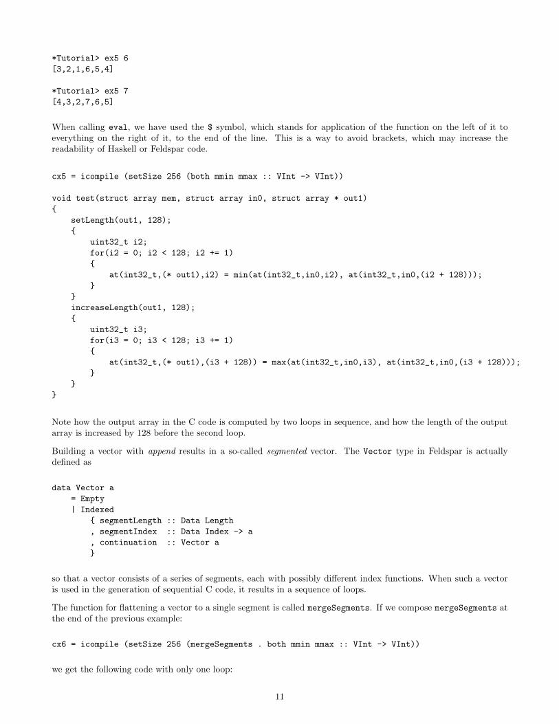
When calling eval, we have used the $ symbol, which stands for application of the function on the left of it toeverything on the right of it, to the end of the line. This is a way to avoid brackets, which may increase thereadability of Haskell or Feldspar code.

cx5 = icompile (setSize 256 (both mmin mmax :: VInt -> VInt))


{


{

uint32_t i2;

for(i2 = 0; i2 < 128; i2 += 1)

{


}

}

increaseLength(out1, 128);

{

uint32_t i3;

for(i3 = 0; i3 < 128; i3 += 1)

{

at(int32_t,(* out1),(i3 + 128)) = max(at(int32_t,in0,i3), at(int32_t,in0,(i3 + 128)));

}

}

}

Note how the output array in the C code is computed by two loops in sequence, and how the length of the outputarray is increased by 128 before the second loop.

Building a vector with append results in a so-called segmented vector. The Vector type in Feldspar is actuallydefined as

data Vector a

= Empty

| Indexed

{ segmentLength :: Data Length

, segmentIndex :: Data Index -> a

, continuation :: Vector a

}

so that a vector consists of a series of segments, each with possibly different index functions. When such a vectoris used in the generation of sequential C code, it results in a sequence of loops.

The function for flattening a vector to a single segment is called mergeSegments. If we compose mergeSegments atthe end of the previous example:

cx6 = icompile (setSize 256 (mergeSegments . both mmin mmax :: VInt -> VInt))

we get the following code with only one loop:

11


{


{

uint32_t i2;

for(i2 = 0; i2 < 256; i2 += 1)

{

uint32_t v3;

v3 = (i2 - 128);

if((i2 < 128))

{


}

else

{

at(int32_t,(* out1),i2) = max(at(int32_t,in0,v3), at(int32_t,in0,(v3 + 128)));

}

}

}

}

For ease, let us restrict out attention to single segment vectors in the forthcoming examples.

When we think of the representation of a vector in terms of an index function, it is not surprising that the functionmap on single segment vectors can be implemented as follows:

map :: (a -> b) -> Vector a -> Vector b

map f (Indexed l ixf Empty) = Indexed l (f . ixf) Empty

The right hand side of the equation could also be written indexed l (f . ixf), which means exactly the samething. We will use this shorter form in future.

It turns out that it is also useful to apply a function before doing the indexing and this is one way to representpermutations of vectors.

premap :: (Data Index -> Data Index) -> Vector a -> Vector a

premap f (Indexed l ixf Empty) = indexed l (ixf . f)

Consider the problem of swapping the odd and even indexed elements of an even-length vector. One could write

swapOE1 :: (Syntactic a) => Vector a -> Vector a

swapOE1 v = indexed (length v) ixf

where

ixf i = condition (i ‘mod‘ 2 == 0) (v!(i+1)) (v!(i-1))

Here, the v! notation indexes into the input vector. The condition construct

condition :: forall a. (Syntactic a) => Data Bool -> a -> a -> a

returns its second parameter if its first is true, and its third otherwise. Note the use of the infix version of themodulus function, indicated by the back-quotes around mod.

The function swapOE1 could be rewritten to separate the index computation into a function to which premap isapplied:

12

swapOE2 :: Vector a -> Vector a

swapOE2 = premap (\i -> condition (i ‘mod‘ 2 == 0) (i+1)(i-1))

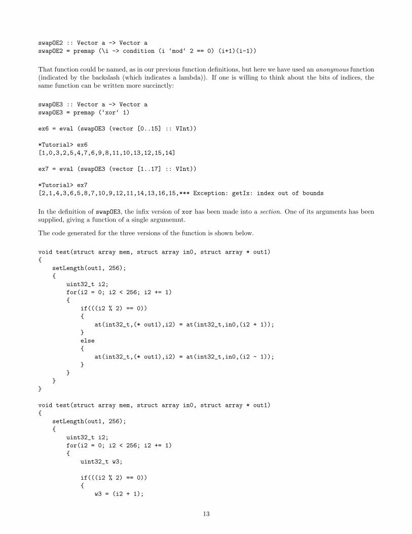
That function could be named, as in our previous function definitions, but here we have used an anonymous function(indicated by the backslash (which indicates a lambda)). If one is willing to think about the bits of indices, thesame function can be written more succinctly:

swapOE3 :: Vector a -> Vector a

swapOE3 = premap (‘xor‘ 1)

ex6 = eval (swapOE3 (vector [0..15] :: VInt))

*Tutorial> ex6

[1,0,3,2,5,4,7,6,9,8,11,10,13,12,15,14]

ex7 = eval (swapOE3 (vector [1..17] :: VInt))

*Tutorial> ex7

[2,1,4,3,6,5,8,7,10,9,12,11,14,13,16,15,*** Exception: getIx: index out of bounds

In the definition of swapOE3, the infix version of xor has been made into a section. One of its arguments has beensupplied, giving a function of a single argumemnt.

The code generated for the three versions of the function is shown below.


{


{

uint32_t i2;

for(i2 = 0; i2 < 256; i2 += 1)

{

if(((i2 % 2) == 0))

{

at(int32_t,(* out1),i2) = at(int32_t,in0,(i2 + 1));

}

else

{

at(int32_t,(* out1),i2) = at(int32_t,in0,(i2 - 1));

}

}

}

}


{


{

uint32_t i2;

for(i2 = 0; i2 < 256; i2 += 1)

{

uint32_t w3;

if(((i2 % 2) == 0))

{

w3 = (i2 + 1);

13

}

else

{

w3 = (i2 - 1);

}

at(int32_t,(* out1),i2) = at(int32_t,in0,w3);

}

}

}


{


{

uint32_t i2;

for(i2 = 0; i2 < 256; i2 += 1)

{

at(int32_t,(* out1),i2) = at(int32_t,in0,(i2 ^ 1));

}

}

}

Exercise 1 Define a function that takes a vector as input and returns those elements that have even index. Theanswer is given in the Appendix.

For single segment vectors, one can define the reverse function as follows:

rev1 :: Vector a -> Vector a

rev1 v = premap (\i -> l-1-i) v

where

l = length v

In the special case of vectors whose length is a power of two, it is also interesting to explore combinators andpermuations that work identically on sub-parts of the vector (and where the definitions specify the length of thosesub-parts but do not mention the overall length of the input vector).

If the length l of a vector or sub-vector is 2k, then taking l − 1 − i has the same effect on the bits of the index ias does complementing the k least significant bits. Take, for instance, k to be 4. Then, complementing the 4 leastsignificant bits of the indices zero to fifteen has the effect of reversing that vector of indices:

ex8 = eval $ map (complN 4)(vector [0..15])

*Tutorial> ex8

[15,14,13,12,11,10,9,8,7,6,5,4,3,2,1,0]

Here, complN k complements the k least significant bits of the index (see Appendix). Note also that if the vectorhas length 2k and we complement fewer than k bits, then we perform the reversal on sub-vectors.

ex9 = eval $ map (complN 2)(vector [0..15])

*Tutorial> ex9

[3,2,1,0,7,6,5,4,11,10,9,8,15,14,13,12]

So, on a non-nested vector whose length is a multiple of 2k, one could represent the function that reverses eachsub-vector of length 2k as follows:

14

revi :: Data Index -> Vector a -> Vector a

revi k = premap (complN k)

ex10 = eval (revi 2 (vector [0..15] :: VInt))

*Tutorial> ex10

[3,2,1,0,7,6,5,4,11,10,9,8,15,14,13,12]

ex11 = eval (revi 2 (vector [0..31] :: VInt))

*Tutorial> ex11

[3,2,1,0,7,6,5,4,11,10,9,8,15,14,13,12,19,18,17,16,23,22,21,20,27,26,25,24,31,30,29,28]

The resulting C code is as one might expect.

cx7 = icompile (setSize 256 (revi 4 . map (+1) :: VInt -> VInt))


{


{

uint32_t i2;

for(i2 = 0; i2 < 256; i2 += 1)

{

at(int32_t,(* out1),i2) = (at(int32_t,in0,(i2 ^ 15)) + 1);

}

}

}

The higher order function fold

A higher order function or combinator commonly used in functional programming is fold, often called reduce. Theversion used in Feldspar has type

fold :: (Syntactic a) => (a -> b -> a) -> a -> Vector b -> a

and it corresponds to Haskell’s foldl. One can think of it as placing an operation between elements of a vector.So, fold (+) 0 gives the sum of all the elements of the vector, while fold (*) 1 gives their product.

ex12 = eval (fold (+) 0 (vector [0..15] :: VInt))

*Tutorial> ex12

120

There is also a variant on fold called fold1 that does not have the initial value, but works only on non-emptyvectors. So, for example, the maximum of a vector is defined as fold1 max.

Exercise 2 Define a function that sums all the elements of a vector of unsigned integers that are even. (Note:Feldspar does not have a filter function like that in Haskell.) The answer is given in the Appendix.

15

pipe, a variant on fold

A structure or pattern of composition that seems to arise often is

f (n-1) . f (n-2) . ... . f 1 . f 0

that is the composition of functions applied to increasing indices (remembering that we need to read from the right).If the input to the pipeline is a, we can write this as

fold (flip f) a (countUp n)

where flip is a standard Haskell function for changing the order of arguments to a function, so that flip f a b = f b a.Indeed, we would like also to have the a input as the final parameter, and this motivates the following definition ofa variant of fold:

pipe :: (Syntactic a) => (Data Index -> a -> a) -> Vector (Data Index) -> a -> a

pipe = flip . fold . flip

The definition of pipe could also have been written as

pipe stage vec init = fold stage’ init vec

where

stage’ a ix = stage ix a

So really we are just making a specialised version of fold with the order of input parameters changed. Now, thepattern that we are trying to capture can be written as

pipe f (countUp n)

A tiny example of the use of pipe is this version of the Factorial function:

fact :: UInt -> UInt

fact i = pipe f (countUp1 i) 1

where

f i = (* i)

which gives the following C code:

void test(struct array mem, uint32_t in0, uint32_t * out1)

{

uint32_t temp2;

(* out1) = 1;

{

uint32_t i3;

for(i3 = 0; i3 < in0; i3 += 1)

{

temp2 = ((* out1) * (i3 + 1));

(* out1) = temp2;

}

}

}

16

Exercise 3a The above Factorial function results in a for-loop that really iterates once too often. Modify thefunction to fix this. The answer is given in the Appendix.

Exercise 3b Feldspar has a variant of fold that does not take an initial value, and assumes a non-empty vectoras input. It is called fold1 and is defined in terms of fold as follows:

fold1 :: Type a => (Data a -> Data a -> Data a) -> Vector (Data a) -> Data a

fold1 f a = fold f (head a) (tail a)

Use this higher order function to define the Factorial function and study the resulting compiled code. The answeris given in the Appendix.

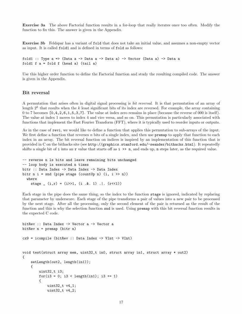
Bit reversal

A permutation that arises often in digital signal processing is bit reversal. It is that permutation of an array oflength 2k that results when the k least significant bits of its index are reversed. For example, the array containing0 to 7 becomes [0,4,2,6,1,5,3,7]. The value at index zero remains in place (because the reverse of 000 is itself).The value at index 1 moves to index 4 and vice versa, and so on. This permutation is particularly associated withfunctions that implement the Fast Fourier Transform (FFT), where it is typically used to reorder inputs or outputs.

As in the case of revi, we would like to define a function that applies this permutation to sub-arrays of the input.We first define a function that reverses n bits of a single index, and then use premap to apply that function to eachindex in an array. The bit reversal function on indices is inspired by an implementation of this function that isprovided in C on the bithacks site (see http://graphics.stanford.edu/~seander/bithacks.html). It repeatedlyshifts a single bit of i into an r value that starts off as i >> n, and ends up, n steps later, as the required value.

-- reverse n ls bits and leave remaining bits unchanged

-- loop body is executed n times

bitr :: Data Index -> Data Index -> Data Index

bitr n i = snd (pipe stage (countUp n) (i, i >> n))

where

stage _ (i,r) = (i>>1, (i .&. 1) .|. (r<<1))

Each stage in the pipe does the same thing, so the index to the function stage is ignored, indicated by replacingthat parameter by underscore. Each stage of the pipe transforms a pair of values into a new pair to be processedby the next stage. After all the processing, only the second element of the pair is returned as the result of thefunction and this is why the selection function snd is used. Using premap with this bit reversal function results inthe expected C code.

bitRev :: Data Index -> Vector a -> Vector a

bitRev n = premap (bitr n)

cx9 = icompile (bitRev :: Data Index -> VInt -> VInt)

void test(struct array mem, uint32_t in0, struct array in1, struct array * out2)

{

setLength(out2, length(in1));

{

uint32_t i3;

for(i3 = 0; i3 < length(in1); i3 += 1)

{

uint32_t v4_1;

uint32_t v4_2;

17

http://graphics.stanford.edu/~seander/bithacks.html

uint32_t temp5_1;

uint32_t temp5_2;

v4_1 = i3;

v4_2 = (i3 >> in0);

{

uint32_t i6;

for(i6 = 0; i6 < in0; i6 += 1)

{

temp5_1 = (v4_1 >> 1);

temp5_2 = ((v4_1 & 1) | (v4_2 << 1));

v4_1 = temp5_1;

v4_2 = temp5_2;

}

}

at(int32_t,(* out2),i3) = at(int32_t,in1,v4_2);

}

}

}

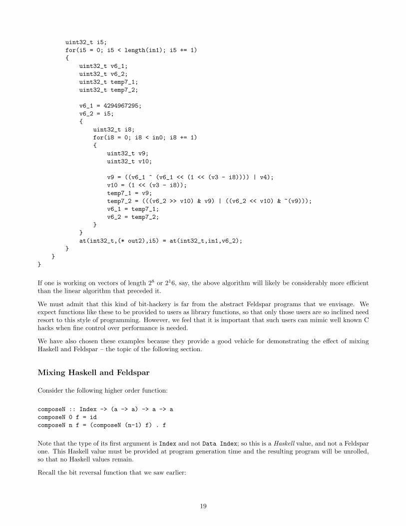
If one knows that the number of bits to be reversed is itself a power of two, one can reduce the number of iterationsneeded from 2n to n by performing that reversal more cleverly. The idea is to first swap the top and bottom 2n−1

bits, then to swap blocks of bits half that size, then a quarter, and so on until one swaps adjacent bits. Thisresults in reversal of the 2n bits. There is doubtless a functional programming oriented solution to the problem ofhow to write such a function (and readers familiar with Haskell might like to try to find it). However, here, wetake inspiration from C bit-hackery again. First, we make the function mergeBy that combines two index valuesaccording to a mask. It “takes from” the first index at the bit positions in which the mask is set, and from thesecond index otherwise.

mergeBy :: Data Index -> Data Index -> Data Index -> Data Index

mergeBy m a b = (a .&. m) .|. (b .&. complement m)

Now, we make clever use of a sequence of masks and of this mergeBy function to do the necessary swapping of bits.The reader might like to figure out what values the variable mask’ has in each of the n iterations of the pipe.

bitrLog :: Data Index -> Data Index -> Data Index

bitrLog n i = snd (pipe stage (map (1<<) (countDown n)) (allOnes, i))

where

stage s (mask, v) = (mask’, mergeBy mask’ (v>>s) (v<<s))

where

mask’ = (mask ‘xor‘ (mask << s)) .|. zeroBitsN (1 << n)

bitRevLog :: Data Index -> Vector a -> Vector a

bitRevLog n = premap (bitrLog n)

cx10 = icompile (bitRevLog :: Data Index -> VInt -> VInt)


{

uint32_t v3;

uint32_t v4;

v3 = (in0 - 1);

v4 = (4294967295 << (1 << in0));


{

18

uint32_t i5;

for(i5 = 0; i5 < length(in1); i5 += 1)

{

uint32_t v6_1;

uint32_t v6_2;

uint32_t temp7_1;

uint32_t temp7_2;

v6_1 = 4294967295;

v6_2 = i5;

{

uint32_t i8;

for(i8 = 0; i8 < in0; i8 += 1)

{

uint32_t v9;

uint32_t v10;

v9 = ((v6_1 ^ (v6_1 << (1 << (v3 - i8)))) | v4);

v10 = (1 << (v3 - i8));

temp7_1 = v9;

temp7_2 = (((v6_2 >> v10) & v9) | ((v6_2 << v10) & ~(v9)));

v6_1 = temp7_1;

v6_2 = temp7_2;

}

}

at(int32_t,(* out2),i5) = at(int32_t,in1,v6_2);

}

}

}

If one is working on vectors of length 28 or 216, say, the above algorithm will likely be considerably more efficientthan the linear algorithm that preceded it.

We must admit that this kind of bit-hackery is far from the abstract Feldspar programs that we envisage. Weexpect functions like these to be provided to users as library functions, so that only those users are so inclined needresort to this style of programming. However, we feel that it is important that such users can mimic well known Chacks when fine control over performance is needed.

We have also chosen these examples because they provide a good vehicle for demonstrating the effect of mixingHaskell and Feldspar – the topic of the following section.

Mixing Haskell and Feldspar

Consider the following higher order function:

composeN :: Index -> (a -> a) -> a -> a

composeN 0 f = id

composeN n f = (composeN (n-1) f) . f

Note that the type of its first argument is Index and not Data Index; so this is a Haskell value, and not a Feldsparone. This Haskell value must be provided at program generation time and the resulting program will be unrolled,so that no Haskell values remain.

Recall the bit reversal function that we saw earlier:

19

bitr :: Data Index -> Data Index -> Data Index

bitr n i = snd (pipe stage (countUp n) (i, i >> n))

where

stage _ (i,r) = (i>>1, (i .&. 1) .|. (r<<1))

Let us replace the pipe by composeN:

bitrH :: Index -> Data Index -> Data Index

bitrH n i = snd (composeN n stage (i, i >> vn))

where

stage (i,r) = (i>>1, (i .&. 1) .|. (r<<1))

vn = value n

bitRevH :: Index -> Vector a -> Vector a

bitRevH n = premap (bitrH n)

Now there is no longer a loop in the calculation of the bit-reversal of a given index.

cx11 = icompile (bitRevH 8 :: VInt -> VInt)


{


{

uint32_t i2;

for(i2 = 0; i2 < length(in0); i2 += 1)

{

uint32_t v3;

uint32_t v4;

uint32_t v5;

v3 = ((((((i2 >> 1) >> 1) >> 1) >> 1) >> 1) >> 1);

v4 = ((((i2 >> 1) >> 1) >> 1) >> 1);

v5 = ((i2 >> 1) >> 1);


= at(int32_t,in0,(((v3 >> 1) & 1) | (((v3 & 1) | ((((v4 >> 1) & 1)

| (((v4 & 1) | ((((v5 >> 1) & 1) | (((v5 & 1) | ((((i2 >> 1) & 1) | (((i2 & 1)

| ((i2 >> 8) << 1)) << 1)) << 1)) << 1)) << 1)) << 1)) << 1)) << 1)));

}

}

}

Exercise 4 Define a function with type

composeList :: [ a -> a ] -> a -> a

that composes a (Haskell) list of functions (rather than n copies of the same function. The answer is given in theAppendix.

The reason we need the composeList function that you have just defined is that we would like to replace the firstData Index parameter to bitrLog with an Index parameter. Recall

bitrLog :: Data Index -> Data Index -> Data Index

bitrLog n i = snd (pipe stage (map (1<<) (countDown n)) (allOnes, i))

20

where


where

mask’ = (mask ‘xor‘ (mask << s)) .|. zeroBitsN (1 << n)

Here, each stage in the pipe does something that depends on the index, so we need to be able to compose a (Haskell)list of possibly different functions. In the bitrLogH function below, that list of functions is fns, which corresponds,informally, to the list [stage(2(n− 1)), stage(2(n− 2)), ..., stage2, stage1]. The definition of what each stage doesremains unchanged.

bitrLogH :: Index -> Data Index -> Data Index

bitrLogH n i = snd (composeList fns (allOnes, i))

where

fns = [stage (1 << (value ix)) | ix <- P.reverse [0..n-1]]


where

mask’ = (mask ‘xor‘ (mask << s)) .|. zeroBitsN (1 << (value n))

bitRevLogH :: Index -> Vector a -> Vector a

bitRevLogH n = premap (bitrLogH n)

Now, when we compile bitRevLogH, we must choose a value for the Index parameter.

cx12 = icompile (bitRevLogH 4 :: VInt -> VInt)


{


{

uint32_t i2;

for(i2 = 0; i2 < length(in0); i2 += 1)

{

uint32_t v3;

uint32_t v4;

uint32_t v5;

v5 = (((i2 >> 8) & 4294902015) | ((i2 << 8) & 65280));

v4 = (((v5 >> 4) & 4294905615) | ((v5 << 4) & 61680));

v3 = (((v4 >> 2) & 4294914867) | ((v4 << 2) & 52428));

at(int32_t,(* out1),i2) = at(int32_t,in0,(((v3 >> 1) & 4294923605) | ((v3 << 1) & 43690)));

}

}

}

More combinators: defining sorters

Let us assume that we wish to sort a vector whose length is a power of 2. Earlier, we saw the function both, whichtook a vector of length 2n and operated on pairs of elements whose indices were n apart. Let us generalise thisidea slightly. We still have the two function parameters, f and g, and a single segment input vector. But we alsohave a parameter that encodes the condition on the index that decides which of f or g is used for a given outputindex. In addition, the p parameter shows how to get from an index to its partner, so that both inputs to one ofthose functions can be provided. If the condition is true of the index being considered, i, f is applied to the valuesat index i and index (p i) of the input vector. If the condition is false, g is applied.

21

comb :: (Syntactic a) =>

(t -> t -> a) -> (t -> t -> a)

-> (Data Index -> Data Bool) -> (Data Index -> Data Index)

-> Vector t

-> Vector a

comb f g c p (Indexed l ixf Empty) = indexed l ixf’

where

ixf’ i = condition (c i) (f a b) (g a b)

where

a = ixf i

b = ixf (p i)

So, for example, the following combinator applies f and g to elements 2k apart:

apart :: (Syntactic a) =>

(t -> t -> a) -> (t -> t -> a)

-> Data Index

-> Vector t

-> Vector a

apart f g k = comb f g (bitZero k) (flipBit k)

ex13 k = eval (apart mmin mmax k (vector [7,6,5,4,3,2,1,0] :: VInt))

ex14 = [ ex13 (value i) | i <- [0..2] ]

*Tutorial> ex14

[[6,7,4,5,2,3,0,1],[5,4,7,6,1,0,3,2],[3,2,1,0,7,6,5,4]]

Here, we use a Haskell list comprehension to express the small tests that we want to run. We would get the sameeffect by running ex6 with parameters 0, 1 and 2 separately. The function value converts a Haskell level value toa Feldspar one. Note how the tests compare adjacent values, values two apart and values four apart respectively.

Batcher’s bitonic merger is a network made from min and max or comparator components that can sort a vectorof 2m inputs. It first compares and swaps elements 2(n − 1) apart, then 2(n − 2) , then 2(n − 2), and so on, untilit is finally comparing adjacent elements. We have the building blocks to describe this: the cominators pipe and!apart!.

-- Batcher’s bitonic merge, 2^n inputs

batMerge :: (P.Ord a, Type a) => Data Index -> DVector a -> DVector a

batMerge n = pipe (apart mmin mmax) (countDown n)

What batMerge n actually does is perform Batcher’s merge on each 2n element block of the input. And the mergeitself actually merges two concatenated input vectors if one is sorted in one direction and the other in the oppositedirection! So if we can make a permutation that reverses the order of half of a sub-array, then we can easily get amerger that merges two concatenated sorted lists. We have seen how to reverse sub-arrays, and reversing only halfof each is similar:

-- works on 2^n length sub-arrays, reversing the second half of each

-- n >= 1

halfRev :: (Type a) => Data Index -> DVector a -> DVector a

halfRev n = premap (\i -> (condition (bitZero n’ i) i (complN n’ i)))

where

n’ = n-1

We can also avoid the condition that results in an if statement by using the bithack introduced earlier:

22

-- works on 2^n length sub-arrays

-- works on 2^n length sub-arrays

halfRev1 :: (Type a) => Data Index -> DVector a -> DVector a

halfRev1 n = premap (\i -> i ‘xor‘ (onCond (bitOne n’ i) (oneBitsN n’)))

where

n’ = n-1

ex15 = [eval (halfRev1 (value k) (vector [0..15] :: VInt)) | k <- [1..4]]

*Tutorial> ex15

[[0,1,2,3,4,5,6,7,8,9,10,11,12,13,14,15],[0,1,3,2,4,5,7,6,8,9,11,10,12,13,15,14]

,[0,1,2,3,7,6,5,4,8,9,10,11,15,14,13,12],[0,1,2,3,4,5,6,7,15,14,13,12,11,10,9,8]]

Now, the following should produce sorted output provided the input consists of two concatenated sorted arrays:

-- merger, 2^n inputs, sorted in top and bottom halves, gives sorted output

merge :: (P.Ord a, Type a) => Data Index -> DVector a -> DVector a

merge n = batMerge n . halfRev1 n

Now, we can use this component, first to sort sub-arrays of length 2, then 4, then 8 and so on. So, this is again apattern that can easily be modelled using pipe.

sortV :: (P.Ord a, Type a) => Data Index -> DVector a -> DVector a

sortV n = pipe merge (countUp1 n)

ex16 k = eval (sortV k (vector [0,1,2,3,12,5,6,7,1,14,13,12,11,19,9,8] :: VInt))

*Tutorial> ex16 3

[0,1,2,3,5,6,7,12,1,8,9,11,12,13,14,19]

*Tutorial> ex16 4

[0,1,1,2,3,5,6,7,8,9,11,12,12,13,14,19]

The resulting code is


{

copyArray(out2, in1);

{

uint32_t i4;

for(i4 = 0; i4 < in0; i4 += 1)

{

uint32_t v5;

uint32_t v6;

uint32_t v7;

uint32_t v8;

v5 = (i4 + 1);

v6 = ~((4294967295 << (v5 - 1)));

v7 = (1 << (v5 - 1));

v8 = (v5 - 1);

setLength(&at(struct array,mem,0), length((* out2)));

{

uint32_t i11;

for(i11 = 0; i11 < length((* out2)); i11 += 1)

{

23

at(int32_t,at(struct array,mem,0),i11)

= at(int32_t,(* out2),(i11 ^ (v6 & -((uint32_t)(((i11 & v7) != 0))))));

}

}

{

uint32_t i10;

for(i10 = 0; i10 < v5; i10 += 1)

{

uint32_t v12;

v12 = (1 << (v8 - i10));

setLength(&at(struct array,mem,1), length(at(struct array,mem,0)));

{

uint32_t i13;

for(i13 = 0; i13 < length(at(struct array,mem,0)); i13 += 1)

{

uint32_t v14;

v14 = (i13 ^ v12);

if(((i13 & v12) == 0))

{


= min(at(int32_t,at(struct array,mem,0),i13),

at(int32_t,at(struct array,mem,0),v14));

}

else

{


= max(at(int32_t,at(struct array,mem,0),i13),


}

}

}

copyArray(&at(struct array,mem,0), at(struct array,mem,1));

}

}

copyArray(out2, at(struct array,mem,0));

}

}

}

In this example code, you can see how the mem parameter is used as a scratchpad in which intermediate arrays arestored. That is the purpose of that parameter.

Note that the halfRev1 permutation cannot fuse with the computations following it because they are inside a loop.One option is to unwind the loop one step, to permit fusion of the permutation with that loop body:

-- sorter on each 2^n length sub-array of inputs, n > 0

-- inside the merger, one loop body is unwound to permit fusion with halfRev1

sort1 :: (P.Ord a, Type a) => Data Index -> DVector a -> DVector a

sort1 n = pipe merge (countUp1 n)

where

merge n = batMerge (n-1) . apart mmin mmax (n-1) . halfRev1 n

Now, the permutation and the first stage of min and !verb!max! functions are fused:

24


{


{

uint32_t i4;

for(i4 = 0; i4 < in0; i4 += 1)

{

uint32_t v5;

uint32_t v6;

uint32_t v7;

uint32_t v8;

v5 = ((i4 + 1) - 1);

v6 = (1 << v5);

v7 = ~((4294967295 << v5));

v8 = (v5 - 1);


{

uint32_t i11;


{

uint32_t v12;

uint32_t v13;

uint32_t v14;

uint32_t v15;

v12 = (i11 & v6);

v13 = (i11 ^ (v7 & -((uint32_t)((v12 != 0)))));

v15 = (i11 ^ v6);

v14 = (v15 ^ (v7 & -((uint32_t)(((v15 & v6) != 0)))));

if((v12 == 0))

{


= min(at(int32_t,(* out2),v13),

at(int32_t,(* out2),v14));

}

else

{


= max(at(int32_t,(* out2),v13),

at(int32_t,(* out2),v14));

}

}

}

{

uint32_t i10;

for(i10 = 0; i10 < v5; i10 += 1)

{

uint32_t v16;

v16 = (1 << (v8 - i10));

setLength(&at(struct array,mem,1), length(at(struct array,mem,0)));

{

uint32_t i17;

for(i17 = 0; i17 < length(at(struct array,mem,0)); i17 += 1)

25

{

uint32_t v18;

v18 = (i17 ^ v16);

if(((i17 & v16) == 0))

{




}

else

{




}

}

}

copyArray(&at(struct array,mem,0), at(struct array,mem,1));

}

}


}

}

}

Memory

We have just seen an example in which the user manipulated her Feldspar source code in order to take advantage ofvector fusion. Is fusion always a good thing? The answer to this is “no”. There are situations in which fusion givesundesired results. We will illustrate this first by unrolling an instance of the batMerge function, to give three stagesof min and max computations. In the resulting code, these three stages are fused, leading to significant repeatedcomputation:

fex = apart mmin mmax 0 . apart mmin mmax 1 . apart mmin mmax 2

cx14 = icompile (fex :: VInt -> VInt)


{


{

uint32_t i2;

for(i2 = 0; i2 < 256; i2 += 1)

{

int32_t v3;

int32_t v4;

uint32_t v5;

int32_t v6;

uint32_t v7;

uint32_t v8;

int32_t v9;

uint32_t v10;

int32_t v11;

uint32_t v12;

26

int32_t v13;

uint32_t v14;

uint32_t v15;

v5 = (i2 ^ 4);

if(((i2 & 4) == 0))

{

v4 = min(at(int32_t,in0,i2), at(int32_t,in0,v5));

}

else

{

v4 = max(at(int32_t,in0,i2), at(int32_t,in0,v5));

}

v7 = (i2 ^ 2);

v8 = (v7 ^ 4);

if(((v7 & 4) == 0))

{

v6 = min(at(int32_t,in0,v7), at(int32_t,in0,v8));

}

else

{

v6 = max(at(int32_t,in0,v7), at(int32_t,in0,v8));

}

if(((i2 & 2) == 0))

{

v3 = min(v4, v6);

}

else

{

v3 = max(v4, v6);

}

v10 = (i2 ^ 1);

v12 = (v10 ^ 4);

if(((v10 & 4) == 0))

{


}

else

{


}

v14 = (v10 ^ 2);

v15 = (v14 ^ 4);

if(((v14 & 4) == 0))

{


}

else

{


}

if(((v10 & 2) == 0))

{

v9 = min(v11, v13);

}

else

27

{

v9 = max(v11, v13);

}

if(((i2 & 1) == 0))

{

at(int32_t,(* out1),i2) = min(v3, v9);

}

else

{

at(int32_t,(* out1),i2) = max(v3, v9);

}

}

}

}

The function force can be used to force the introduction of intermediate vectors between our three stages. Apartfrom causing the introduction of storage, force acts like the identity function. When we place force between eachof the three stages, we then get three separate loops, with intermediate values stored in two additional arrays (andthe mem parameter is used for this purpose, containing the two arrays at index 0 and index 1.).

fexforce :: (P.Ord a, Type a) => DVector a -> DVector a

fexforce = apart mmin mmax 0 . force .

apart mmin mmax 1 . force .

apart mmin mmax 2

cx15 = icompile (setSize 256 (fexforce :: VInt -> VInt))


{

setLength(&at(struct array,mem,1), 256);

{

uint32_t i4;

for(i4 = 0; i4 < 256; i4 += 1)

{

uint32_t v5;

v5 = (i4 ^ 4);

if(((i4 & 4) == 0))

{


= min(at(int32_t,in0,i4),

at(int32_t,in0,v5));

}

else

{


= max(at(int32_t,in0,i4),

at(int32_t,in0,v5));

}

}

}


{

uint32_t i6;

for(i6 = 0; i6 < 256; i6 += 1)

{

28

uint32_t v7;

v7 = (i6 ^ 2);

if(((i6 & 2) == 0))

{




}

else

{




}

}

}


{

uint32_t i8;

for(i8 = 0; i8 < 256; i8 += 1)

{

uint32_t v9;

v9 = (i8 ^ 1);

if(((i8 & 1) == 0))

{




}

else

{




}

}

}

}

The following examples of simple filters again illustrate the same principle. Fusion is not always what one wants,and the use of force provides a way to trade off repeated computation and space. The reader should compare thecode produced for bandPass1 and bandPass2.

-- | First-order FIR filter

fir1 :: Data Float -> Data Float -> DVector Float -> DVector Float

fir1 a0 a1 vec = map (\(x,y) -> a0*x + a1*y) $ zip vec (tail vec)

lowPass :: Data Float -> DVector Float -> DVector Float

lowPass x = fir1 x (1-x)

highPass :: Data Float -> DVector Float -> DVector Float

highPass x = fir1 x (x-1)

bandPass1 :: Data Float -> DVector Float -> DVector Float

29

bandPass1 x = highPass x . lowPass x

bandPass2 :: Data Float -> DVector Float -> DVector Float

bandPass2 x = highPass x . force . lowPass x

cx16 = icompile (setSize 256 (lowPass 0.5))


{


{

uint32_t i2;

for(i2 = 0; i2 < 255; i2 += 1)

{

at(float,(* out1),i2)

= ((0.5f * at(float,in0,i2)) + (0.5f * at(float,in0,(i2 + 1))));

}

}

}

cx17 = icompile (setSize 256 (highPass 0.5))


{


{

uint32_t i2;

for(i2 = 0; i2 < 255; i2 += 1)

{


= ((0.5f * at(float,in0,i2)) + (-0.5f * at(float,in0,(i2 + 1))));

}

}

}

cx18 = icompile (setSize 256 (bandPass1 0.5))


{


{

uint32_t i2;

for(i2 = 0; i2 < 254; i2 += 1)

{

float v3;

v3 = (0.5f * at(float,in0,(i2 + 1)));


= ((0.5f * ((0.5f * at(float,in0,i2)) + v3)) +

(-0.5f * (v3 + (0.5f * at(float,in0,((i2 + 1) + 1))))));

}

}

}

cx19 = icompile (setSize 256 (bandPass2 0.5))

30


{


{

uint32_t i3;

for(i3 = 0; i3 < 255; i3 += 1)

{

at(float,at(struct array,mem,0),i3)

= ((0.5f * at(float,in0,i3)) + (0.5f * at(float,in0,(i3 + 1))));

}

}


{

uint32_t i4;

for(i4 = 0; i4 < 254; i4 += 1)

{


= ((0.5f * at(float,at(struct array,mem,0),i4)) +

(-0.5f * at(float,at(struct array,mem,0),(i4 + 1))));

}

}

}

It is important to realise that using fold, fold1 or functions related to them (such as pipe) also introducesintermediate storage (to store the accumulating parameter). There is an implicit force at the end of the functionbeing folded. In the case of the function batMerge, we have just seen that we actually wanted those instances offorce in order to avoid repeated computation – so it was just as well that we expressed the computation using afold. However, one should be careful, in general, about having vectors as the inputs and outputs of folds. Forexample, returning to the bit reveral function, one way to express it is as a composition of perfect shuffles ofincreasing size. A perfect shuffle takes a vector of length 2k, halves it and interleaves the two halves (rather as acard player does with a deck of cards before dealing). Thus, applying the perfect shuffle to the vector containingzero to fifteen should give the following vector:

*Tutorial> ex17

[0,8,1,9,2,10,3,11,4,12,5,13,6,14,7,15]

To encode this, we define a function riffle that acts in this way on sub-vectors of length 2k.

riffle :: Data Index -> Vector a -> Vector a

riffle k = premap (rotBitFrom0 k)

The least significant bit of the index is moved to position k, while bits 1 to k all move one position rightwards (topositions 0 to k − 1). Now one way to perform bit reversal is to apply a sequence of riffles in what should by nowbe becoming a familiar pattern:

bitRev1 :: Type a => Data Index -> Vector (Data a) -> Vector (Data a)

bitRev1 n = pipe riffle (countUp1 n)

For some purposes, such as reasoning about the algebraic properties of combinators used to build butterfly struc-tures like the bitonic merge, this is a good specification of bit reversal. However, the resulting code uses intermediatestorage when applying the bit reversal permutation – something that was not necessary in out previous implemen-tations. The reason for this is the fact that bitRev1 is defined as a pipe of permutations that work on the wholevector, whereas the earlier versions performed the loop on the indices. It is important to understand this distinction.If possible, one should avoid having a vector as the accumulating parameter in a fold or pipe.

31

cx20 = icompile (bitRev1 :: Data Index -> VInt -> VInt)


{


{

uint32_t i4;

for(i4 = 0; i4 < in0; i4 += 1)

{

uint32_t v5;

uint32_t v6;

uint32_t v7;

v5 = ((4294967295 << (i4 + 1)) << 1);

v6 = (i4 + 1);

v7 = ~(v5);


{

uint32_t i8;


{


= at(int32_t,(* out2),(((i8 & v5) | ((i8 & 1) << v6)) | ((i8 & v7) >> 1)));

}

}


}

}

}

FFT

The structure of the calculation of the Fast Fourier Transform is actually very similar to that of the bitonic mergethat we coded as batMerge. The twiddle factors, however, complicate things slightly. We define a generalisationof the combinator comb that we used earlier in defining apart and the bitonic merge. Below, we first repeat thedefinition of comb and then show how combx adds an additional parameter to allow us to deal with twiddle factors(or more generally with additional calculations that must be different at different array indices).

comb :: (Syntactic a) =>

(t -> t -> a) -> (t -> t -> a)

-> (Data Index -> Data Bool) -> (Data Index -> Data Index)

-> Vector t

-> Vector a

comb f g c p (Indexed l ixf Empty) = indexed l ixf’

where

ixf’ i = condition (c i) (f a b) (g a b)

where

a = ixf i

b = ixf (p i)

combx f g c p x (Indexed l ixf Empty) = indexed l ixf’

where

ixf’ i = condition (c i == 0) (f ai pi xi) (g pi ai xi)

32

where

ai = ixf i

pi = ixf (p i)

xi = x i

Now, the FFT is just pipe stage (countDown l), just as the bitonic merge was. The difference is that each stagein the pipe uses the combx combinator. The two functions that are chosen between at any given index and stage(and depending on a particular bit in the index) are addition and a combination of subtraction and mulitplicationby a twiddle factor.

fft :: Data Index -> DVector (Complex Float) -> DVector (Complex Float)

fft l = pipe stage (countDown l)

where

stage k = combx f g (bitZero k) (‘xor‘ p) twid

where

p = 1<<k

f a b _ = a + b

g a b t = t * (a-b)

twid i = cis (-pi*(i2f (lsbsN k i)) / i2f p)


{

uint32_t v3;

v3 = (in0 - 1);


{

uint32_t i5;

for(i5 = 0; i5 < in0; i5 += 1)

{

uint32_t v6;

uint32_t v7;

float v8;

v6 = (1 << (v3 - i5));

v7 = ~((4294967295 << (v3 - i5)));

v8 = (float)(v6);


{

uint32_t i9;


{

uint32_t v10;

v10 = (i9 ^ v6);

if(((i9 & v6) == 0))

{

at(float complex,at(struct array,mem,0),i9)

= (at(float complex,(* out2),i9) + at(float complex,(* out2),v10));

}

else

{

at(float complex,at(struct array,mem,0),i9)

= (cis_fun_float((0.0f - ((3.1415927410125732f * (float)((i9 & v7))) / v8)))

* (at(float complex,(* out2),v10) - at(float complex,(* out2),i9)));

}

33

}

}


}

}

}

The inverse FFT is defined almost identically. Only the sign of the exponent in the twiddle factor calculationchanges.

-- 2^l input IFFT. Produces output in bit reversed order.

ifft :: Data Index -> DVector (Complex Float) -> DVector (Complex Float)

ifft l = map (/ (complex (i2f (2^l)) 0)) . pipe stage (countDown l)

where

stage k = combx f g (bitZero k) (‘xor‘ p) twid

where

p = 1<<k

f a b _ = a + b

g a b t = t * (a-b)

twid i = cis (pi*(i2f (lsbsN k i)) / i2f p)

Matrices

The vectors that we have seen so far are one dimensional. While this is a very useful abstraction, it is also importantto have higher dimensional vectors. Matrices, that is two dimensional vectors, are ubiquitous in linear algebra andtherefore in many signal processing applications. Because of the importance of matrices, Feldspar provide a specialmatrix library.

To construct matrices there is a function similar to the function indexed in the vector library. For matrices itis called indexedMat. It takes two lengths to determine the dimension of the array, and an index function whichcomputes the elements based on their indices in the matrix. A simple but useful example of using indexedMat isto define the identity matrix:

idMat n = indexedMat n n (\y x -> x == y ? (1,0))

DCT

As an example of the use of the matrix library we show a simple implementation of (the most common form of)the discrete cosine transform (DCT). We will concentrate on an implementation which is close to the specificationof DCT. (The material we covered on FFT carries over to a large extent to DCT.)

DCT is often expressed such that each element in the output vector is a sum of the input elements multiplied byappropriate factors. This can be succinctly expressed as a matrix multiplication, with the factors being the elementsin the matrix. The function dct2 illustrates the use of this idea in Feldspar.

dct2 :: (DVector Float) -> (DVector Float)

dct2 xn = mat *** xn

where mat = indexedMat (length xn) (length xn) (\k l -> dct2nkl (length xn) k l)

--- Helper function defining all the values in the DCT--2n matrix

dct2nkl :: Data Length -> Data DefaultWord -> Data DefaultWord -> Data Float

dct2nkl n k l = cos ( (k’ * (2 * l’ +1) * pi)/(2 * n’) )

34

where n’ = i2f n

k’ = i2f k

l’ = i2f l

The dct2 function is essentially just a matrix multiplication and a call to indexedMat to create the matrix. Thehelper function dct2nkl is used to compute the elements of the array.

Lowpass filter

lowPassCore :: (Numeric a) => Data Index -> DVector a -> DVector a

lowPassCore k v = take k v ++ replicate x (length v - k) 0

lowPass :: Data Index -> DVector Float -> DVector Float

lowPass k = frequencyTrans (lowPassCore k)

frequencyTrans :: (DVector (Complex Float) -> DVector (Complex Float))

-> DVector Float -> DVector Float

frequencyTrans innerFunction v

= map realPart $ ifft

$ innerFunction

$ fft $ map (\a -> complex a 0) v

Crypto Example

This example is currently provided without comment.

Blake crypto

type MessageBlock = DVector Word32 --- 0..15 type Round = Data Index

type State = Matrix Word32 --- 0..3 0..3

co :: DVector Word32 co = vector

[0x243F6A88,0x85A308D3,0x13198A2E,0x03707344,

0xA4093822,0x299F31D0,0x082EFA98,0xEC4E6C89,

0x452821E6,0x38D01377,0xBE5466CF,0x34E90C6C,

0xC0AC29B7,0xC97C50DD,0x3F84D5B5,0xB5470917]

sigma :: Matrix Index sigma = matrix

[[0,1,2,3,4,5,6,7,8,9,10,11,12,13,14,15]

,[14,10,4,8,9,15,13,6,1,12,0,2,11,7,5,3]

,[11,8,12,0,5,2,15,13,10,14,3,6,7,1,9,4]

,[7,9,3,1,13,12,11,14,2,6,5,10,4,0,15,8]

,[9,0,5,7,2,4,10,15,14,1,11,12,6,8,3,13]

,[2,12,6,10,0,11,8,3,4,13,7,5,15,14,1,9]

,[12,5,1,15,14,13,4,10,0,7,6,3,9,2,8,11]

,[13,11,7,14,12,1,3,9,5,0,15,4,8,6,2,10]

,[6,15,14,9,11,3,0,8,12,2,13,7,1,4,10,5]

,[10,2,8,4,7,6,1,5,15,11,9,14,3,12,13,0] ]

blakeRound :: MessageBlock -> State -> Round -> State

blakeRound m state r =

invDiagonals $

zipWith (g m r) (4 ... 7) $

35

diagonals $

transpose $

zipWith (g m r) (0 ... 3) $

transpose $

state

g :: MessageBlock -> Round -> Data Index -> DVector Word32 -> DVector Word32

g m r i v = fromList [a’’,b’’,c’’,d’’]

where [a,b,c,d] = toList 4 v

a’ = a + b + (m!(sigma!r!(2 * i)) ⊕ (co!(sigma!r!(2 * i+1))))

d’ = (d ⊕ a’) >> 16

c’ = c + d’ b’ = (b ⊕ c’) >> 12

a’’ = a’ + b’ + (m!(sigma!r!(2 * i+1)) ⊕ (co!(sigma!r!(2 * i))))

d’’ = (d’ ⊕ a’’) >> 8

c’’ = c’ + d’’

b’’ = (b’ ⊕ c’’) >> 7

diagonals :: Type a => Matrix a -> Matrix a

diagonals m = map (diag m) (0 ... (length (head m) - 1))

diag :: Type a => Matrix a -> Data Index -> Vector (Data a)

diag m i = zipWith lookup m (i ... (l + i))

where l = length m - 1

lookup v i = v ! (i ‘mod‘ length v)

invDiagonals :: Type a => Matrix a ->

Matrix a invDiagonals m = zipWith shiftVectorR (0 ... (length m - 1)) (transpose m)

shiftVectorR :: Syntactic a => Data Index

-> Vector a -> Vector a shiftVectorR i v

= reverse $ drop i rev ++ take i rev where rev = reverse v

fromList :: Type a => [Data a] -> DVector

a fromList ls = unfreezeVector’ (value len) (loop 1 (parallel

(value len) (const (Prelude.head ls)))) where loop i arr \textbar{}

i Prelude.\textless{} len = loop (i+1) (setIx arr (value i) (ls !!

(fromIntegral i))) \textbar{} otherwise = arr len = fromIntegral

(Prelude.length ls)

toList :: Type a => Index -> Vector (Data

a) -> [Data a] toList n v@(Indexed l ix _) =

Prelude.map (v!) $ Prelude.map value [0..n--1]

Streams

The stream library provide a data type for infinite sequences of values. The type of streams is a useful abstractionfor computations that need to happen in sequence. An important example of such computations is filters, wherelater values depend on earlier one. This is in contrast to vectors, where each element is computed independently ofall the other ones.

To get access to the stream library simply import the module Feldspar.Stream.

Note that some of the functions in the stream libray have the same names as functions in the vector library. If youneed to use both the vector library and the stream library is it best to import one of the qualified. Typically youwill want to import the library that you use most frequently the normal way, without qualified import. For the

36

library that you use more sparingly, use qualified import. For example, if you’re using the vector library quite a lotand the stream library only occasionally then the following import statements might suit you.

import Feldspar.Vector

import qualified Feldspar.Stream as S

Qualifying the stream library like above means that every all stream functions now must be called using a S. prefix.In the rest of this section we will assume that the stream library is imported without qualification to simplify thecode examples.

Constructing simple streams.

To begin with , let us consider some examples of functions that construct streams. Perhaps the simplest suchfunction is repeat:

repeat :: Syntactic a => a -> Stream a

The stream that repeat produces contains an endless repetition of the element given as the first argument.

To produce stream with a little more variation in them the function iterate is useful.

iterate :: Syntactic a => (a -> a) -> a -> Stream a

The call iterate f a will create a stream were f is successively applied to a, i.e. a, f a, f (f a) .... A simpleexample of using iterate is to define the stream of natural numbers, which can be written as iterate (+1) 0

While iterate is already powerful enough to produce non-trivial streams there are still examples that are awkwardto express using it. An even more powerful combinator for producing streams is unfold:

unfold :: (Syntactic a, Syntactic c) => (c -> (a,c)) -> c -> Stream a

The power of unfold comes from the fact that it passes around a state. The second argument to unfold is theinitial state. The first argument is used to produce a new element in the stream from the current state and alsothe next state.

Using streams

Streams are not first class citizens in Feldspar. They can not be compiled as is, they cannot be stored in arrays andthey cannot be the result of a for loop or a conditional expression. The reason for these restrictions is simply thatstreams represent potentially inifinite number of values. So, when we wish to use a stream we must always take outa finite part of it, for example the 20 first elements.

The function used to take a prefix of a stream is aptly named take

take :: (Type a) => Data Length -> Stream (Data a) -> Data [a]

The call take n str takes n elements from the stream str and returns these elements in an array.

The function take is an excellent tool for experimenting with stream programs. Since it is not possible to evaluatea stream directly a simple technique is to extract the first couple of elements of the stream. For example, if we wishto examine the stream of natural numbers that we defined using iterate above we can write like this:

37

> eval $ take 20 (iterate (+1) (0 :: Data Word32))

[0,1,2,3,4,5,6,7,8,9,10,11,12,13,14,15,16,17,18,19]

A type signature has been added to fix the type of the numbers in the stream. Without it, the Haskell interpreterwould complain.

When using streams in actual programs using take is usually not enough. A common pattern is that a vector needsto be considered as a stream and once the stream processing is done it should be converted back to a vector. Tosimplify this kind of patterns the stream library provides the function streamAsVector:

streamAsVector :: (Type a, Type b) =>

(Stream (Data a) -> Stream (Data b))

-> (Vector (Data a) -> Vector (Data b))

This function can be used to conveniently apply a function on streams on a vector. The resulting vector will alwaysbe as long as the input vector. Although this works in many cases there are times when it is necessary to have theoutput vector be of a different size than the input vector. One example is when using stream functions with delayssuch as filters, as we will see in coming sections. For such functions there is the streamAsVectorSize functionwhich has an extra argument compared to streamAsVector.

streamAsVectorSize :: (Type a, Type b) =>

(Stream (Data a) -> Stream (Data b))

-> (Data Length -> Data Length)

-> (Vector (Data a) -> Vector (Data b))

The extra argument is a function which is used to compute the length of the output vector given the size of theinput vector.

Fusion

One of the most useful things about the vector library was that it supported fusion, meaning that all intermediatevector will be optimized away. This is a very nice feature to have as it means that we can write abstract well-structured code without taking the performance it that it normally incurrs in most programming languages.

The stream library also supports fusion. We will illustrate it with a small example.

Suppose we want to have a stream which is a sampling of the sine curve. Below is how we could write one usingthe function unfold. We give the stream an argument so that we can control the number of samplings per period.

sineStream :: Data Length -> Stream (Data Float)

sineStream n = unfold step 0

where step i = (sin ((i2f i) * period), (i+1) ‘mod‘ n)

period = 2 * pi / (i2f n)

Writing the function like this works OK. But there are quite a few things going on at the same time and it mightbe a good idea to isolate them, especially if we can factor out things that are reusable.

Here’s an example of how one can write the same stream but in a more compositional style:

sampleCircle n = map (\i -> 2* pi * i2f i / i2f n)

$ cycle (0...(n-1))

sineStream n = map sin (sampleCircle n)

38

We’ve factored out a function called sampleCycle which generates samplings of the numbers between 0 and 2πover and over. This stream is useful if we were to define a cosineStream. In defining sampleCycle we’ve usedthe function cycle which takes a vector and repeats it indefinitely to create a stream. The map function appliesa function to each element in the stream (much like the function with the same name for vectors). In the case ofsampleCircle it maps a number from 0 to n− 1 to a point on the circle.

Once we have defined sampleCircle it is an easy task to define sineStream by simply mapping the sine function.

If we look at the generated code for these two versions of sineStream (using the take) we see that the code is verysimilar.

Filters

Filters are common in signal processing applications and we will look at how they can be defined in Feldspar usingstreams.

In mathematics filters are most often expressed using recurrence equations. For example,

In the stream library there are combinators for writing recurrence equations that produces streams. These combi-nators are all quite similar but serve slightly different purposes. Perhaps the simplest of the recurrence combinatorsis recurrenceO. The capital O is part of the naming convension for recurrence combinators. It mean that therecurrence equation will refer to previous outputs of the recurrence. To understand recurrenceO let’s look at it’stype:

recurrenceO :: Type a => DVector a -> (DVector a -> Data a) -> Stream (Data a)

The combinator recurrenceO takes two arguments. The first argument is a vector which contains the initial outputsof the stream. The reason for providing initial inputs in a vector is that the recurrence will refer to previous outputs.But initially no outputs have been generated and so without the vector of initial outputs there would have beennothing to compute with.

The second argument to recurrenceO is a function for computing the next element in a stream. It takes as argumenta vector of the most recent previous outputs of the stream. The length of the vector will be the same as the vectorgiven in the first argument. Hence, the first argument is also used to control how many previous outputs can beused when describing the recurrence.

A simple but instructive example of a recurrence equation is to define the fibonacci sequence. Recall that inmathematics the fibonacci sequence is defined as follows:

fib0 = 0fib1 = 1fibn = fibn−1 + fibn−2

The first two elements of the fibonacci sequence are zero and one. After that elements are generated by adding thetwo previous elements in the sequence.

We can express this in Feldspar using recurrenceO as follows:

fib = recurrenceO (vector [0,1]) (\fib -> fib!0 + fib!1)

The initial outputs are zero and one which is why we provide them in the vector.

The second argument is the function used to describe the general case for computing the next element in thesequence. The argument to the function is a vector with the two previous elements of the sequence. Note that, aswith all vectors, the input vector is zero indexed, so the first previous element in the stream is at index zero. This

39

has the consequence that the sequence of elements in the vector is reverse compared to the order in which they arepresented in the output sequence.

The body of the function is simply an addition of two previous elements in the stream. It is nice to compare thefeldspar implementation of fib with the mathematical description. Then are identical modulo syntax.

Note that the above definition of fib is overloaded, it can work with many different kinds of numeric types. If wewant to use them you must specify what type we want the result to have. Alternatively, if we always want to usefib at a particular type we can add a type signature like so:

fib = recurrenceO (vector [0,1 :: Word32]) (\fib -> fib!0 + fib!1)

Trying out the fib stream on the command line produces the familiar sequence of numbers.

> eval $ take 20 fib

[0,1,1,2,3,5,8,13,21,34,55,89,144,233,377,610,987,1597,2584,4181]

Some recurrences are defined using an input stream. For such recurrences recurrenceO is clearly not enough as ithas no notion of input. In the stream library there are several recurrence combinators which can take streams asinput. The simplest one is recurrenceI. Again, the capital I is part the naming convention, meaning that it takesan input and that the recurrence equation may refer to previous inputs. The type of recurrenceI is as follows:

recurrenceI :: (Type a, Type b) => DVector a -> Stream (Data a)

-> (DVector a -> Data b) -> Stream (Data b)

The first two arguments of recurrenceI relates to the input stream. The second argument is the actual inputstream whereas the first argument is a vector of length n which defines the first n values of the input stream whenwe use it in the recurrence equation. The recurrence equation needs to refer to many previous values from the inputstream and those are not available initially. Those values are taken from the vector instead.

The third argument is used to describe the recurrence equation much like with recurrenceI. The difference beingthat the input vector to the function refers to previous input values, not output values.

A simple example of using recurrenceI is the sliding average of a stream. The sliding average can be used to smoothout data from temporary irregularities and spikes. For instance, the seven day sliding average of the number ofcommits to a software project gives a good feel for how much work is done on a weekly basis without the distractionof difference between individual work days. Using the recurrenceI combinator we can write sliding average asfollows:

slidingAvg :: Data DefaultWord -> Stream (Data DefaultWord)

-> Stream (Data DefaultWord)

slidingAvg n str = recurrenceI (replicate n 0) str

(\input -> sum input ‘quot‘ n)

The function slidingAvg takes to arguments: n the number of elements to average, and str, the input stream.The body of the function is simply a call to recurrenceI. The first argument is a vector of n zeroes, which aretaken as the first elements of the input stream to average. The second argument is the input stream we wish toprocess.

The third argument to recurrenceI in the definition of slidingAvg is is used to compute the actual averages.Computing the average is straight forward: sum the vector and divide it with its length. The sum function used isdefined in the vector library.

A typical use of recurrences in digital processing is in the description of finite impulse response filters, or FIR filtersfor short. FIR filters are defined in terms of an input stream x, an output stream y, and a vector of filter coefficients

40

b. Lastly, a FIR filter has an order, N, which dictates how many previous input elements it uses. N also dictates thelength of the vector b. Using these components, a FIR filter is described by the following formula:

y[n] =

N∑i=0

bix[n− i]

The summation is simply a scalar product of the vector b and the reverse of x.

We can express FIR filters using the recurrenceI combinator:

fir b input = recurrenceI (replicate n 0) input

(\input -> scalarProd b input)

where n = length b

The function fir takes two arguments: the coefficient vector b and the input stream which we called x above. Wedo not take N as a parameter, instead we use the fact that it can be derived from the length of b.

The body of fir is simply a call to recurrenceI with the appropriate arguments. We set the initial input vectorto be zeroes. The vector has size n since that determines how many previous input values which can be used inthe filter. The second argument to recurrenceI is simply the input stream. Finally, the third argument describesthe equation for FIR filters. We use the function scalarProd from the vector library. Note that we don’t have toreverse the vector of inputs as it is already provided in reverse order.

A more powerful type of filters compared to FIR filters are infinite impulse response filters (IIR filters). IIR filtersare typically described using the following formula:

y[n] =1

a0(

P∑i0

bix[n− 1] −Q∑

j=1

ajy[n− j])

The left summation is similar to the formula for FIR filters, except that instead of N we use P which is the idiomfor IIR filters. P is referred to as the feedforward filter order and thus b is now referred to as the feedforward filtercoefficients. The right summation is the feedback part where Q is the feedback filter order and a is the vector offeedback filter coefficients. Again, we note that the two summations are simply scalar products.

The crucial difference with IIR filter is that the recurrence equation can refer to both previous inputs and previousoutputs. The recurrence combinators we have shown so far cannot handle this. Therefore the stream libraryprovides recurrenceIO which provides functionality which supercedes both recurrenceO and recurrenceI. It’stype is naturally more complicated but should look familiar compared to the types of the simpler recurrencecombinators:

recurrenceIO :: (Type a, Type b) => DVector a -> Stream (Data a) -> DVector b

-> (DVector a -> DVector b -> Data b) -> Stream (Data b)

The two first argument relates to the input stream: the second argument is the actual stream and the first argumentis the associated vector. The third argument contains the initial outputs and the fourth element is the function fordescribing the recurrence.

Using the recurrenceIO combinator we can now write an IIR filter in Feldspar:

iir a0 a b input = recurrenceIO (replicate q 0) input (replicate p 0)

(\input output -> 1 / a0 * (scalarProd b input

- scalarProd a output))

where p = length b

q = length a

Hopefully the pattern should be familiar now; we will not explain the iir function in detail.

41

Fixed point arithmetic

The Feldspar.FixedPoint module provides the Fix type for computations on fixed point platforms. In Feldspar,one can implement a generic algorithm and create wrappers to transform it to a program using the desired arithmetic,for example:

• floating point arithmetic

• fixed point arithmetic

• emulated floating point arithmetic using integers

This setup makes code easier to write and maintain. On fixed point platforms it also saves the programmer fromhaving to keep the exponents and needed shift operations in mind, as these are calculated automatically.

A toy example is the following where one adds 3.14 to each element of a vector:

generic :: (Fractional a) => Vector a -> Vector a

generic = map (\x -> x+3.14)

The floating point wrapper is easy, it just fixes the type variable a in the generic function to Float:

floating :: DVector Float -> DVector Float

floating = generic

When compiled, this produces C code using floating point arithmetic:


{


{

uint32_t i2;

for(i2 = 0; i2 < length(in0); i2 += 1)

{

at(float,(* out1),i2) = (at(float,in0,i2) + 3.140000104904175f);

}

}

}

The fixed point wrapper is a function from an integer vector to an integer vector, where each integer encodes a realvalue according to a given exponent. The wrapper below states that the exponents of the input and output vectorsare (−4) and (−6) respectively. That is, an integer n in the input vector encode n· 2(−4), and an integer m in theresult vector means m· 2(−6). The functions unfreezeFix’ and freezeFix’ are used to convert between integersand symbolic fixed point numbers. These are mapped to the input and result vectors to achive the conversion ofall elements.

fixed :: DVector Int32 -> DVector Int32

fixed = map (freezeFix’ (-6)) . generic . map (unfreezeFix’ (-4))

This generates the following fixed point C code:

42


{


{

uint32_t i2;

for(i2 = 0; i2 < length(in0); i2 += 1)

{

at(int32_t,(* out1),i2) = ((at(int32_t,in0,i2) + 50) << 2);

}

}

}

One can observe that the floating point value 3.14 from the generic algorithm is converted to the integer value50 using an automatically calculated exponent. The result of the addition is automatically shifted to fulfill thespecified output exponent (−6).

Note that currently only simple heuristics are used when deriving exponents. There is no protection against overflowor loss of precision.

If one does not fix the input and output exponents in the wrapper statically, can use the Fix type instead. Fix

needs one type argument that specifies the mantissa’s type. It is Int16 in the following wrapper.

emulation :: Vector (Fix Int16) -> Vector (Fix Int16)

emulation = generic

In this case exponents are unknown at compilation time. Therefore the resulting C code uses dynamic exponentsand will emulate floating point arithmetic. The type (Fix Int16) is compiled to the following C struct, where thefields member1 and member2 store the exponent and the mantissa respectively.

struct s_int32_t_int16_t_ {

int32_t member1;

int16_t member2;

};

Note that this emulation will compile all heuristics about deriving the exponents and shift operations into the Ccode.

Branches returning fixed point values and loops with fixed point accumulator are to be handled in a special waydue to a technical limitation (that is expected to be solved in release 0.5). A fixed point wrapper created aroundan algorithm involving such constructs is compilable, but will result in C code using dynamic exponents. In orderto get the desired fixed point C code with mantissas only, the operator (?!) should be used for branching and thefixFold function for accumulation. A generic algorithm using these constructs is still wrappable in any of the threeways discussed above. An example is scalar product with the following generic algorithm.

scalarProduct :: (Num a, Syntactic a, Fixable a) =>

Data DefaultInt -> Vector a -> Vector a -> a

scalarProduct e xs ys = fixFold (+) (fix e 0) $ zipWith (*) xs ys

Here fixFold is used for summation. When compiling this program for a fixed point platform, the exponent ofthe initial value will be used throughout the whole loop. For this reason the exponent of the initial value is setexplicitly: fix e 0. Adding this exponent e as an additional parameter makes the scalarProduct function moreflexible.

In the floating point wrapper the exponent does not matter, it is even possible to pass undefined.

floatScalarProduct :: DVector Float -> DVector Float -> Data Float

floatScalarProduct = scalarProduct undefined

43

This wrapper generates the following C function.

void test(struct array mem, struct array in0, struct array in1, float * out2)

{

uint32_t v3;

uint32_t v4;

float temp6;

uint32_t w5;

v3 = length(in1);

v4 = length(in0);

if((v3 < v4))

{

w5 = v3;

}

else

{

w5 = v4;

}

(* out2) = 0.0f;

{

uint32_t i7;

for(i7 = 0; i7 < w5; i7 += 1)

{

temp6 = ((* out2) + (at(float,in0,i7) * at(float,in1,i7)));

(* out2) = temp6;

}

}

}

The fixed point wrapper has the following form.

fixScalarProduct :: DVector Int32 -> DVector Int32 -> Data Int32

fixScalarProduct xs ys = freezeFix’ (-18) $ scalarProduct (-16) xs’ ys’

where

xs’ = map (unfreezeFix’ (-8)) xs

ys’ = map (unfreezeFix’ (-6)) ys

It yields the following C code.

void test(struct array mem, struct array in0, struct array in1, int32_t * out2)

{

uint32_t v3;

uint32_t v4;

int32_t w5;

int32_t temp7;

uint32_t w6;

v3 = length(in1);

v4 = length(in0);

if((v3 < v4))

{

w6 = v3;

}

else

44

{

w6 = v4;

}

w5 = 0;

{

uint32_t i8;

for(i8 = 0; i8 < w6; i8 += 1)

{

temp7 = (((w5 >> 2) + (at(int32_t,in0,i8) * at(int32_t,in1,i8))) << 2);

w5 = temp7;

}

}

(* out2) = (w5 << 2);

}

Conclusion

The final version of the tutorial will contain many more examples, including some slightly larger ones. Suggestionsfor examples that would be interesting are solicited.

Acknowledgements

Sheeran’s participation in the Feldspar project during 2009 and 2010 was funded by the Swedish Foundation forStrategic Research under the Strategic Mobility Scheme. The Feldspar project is an initiative of and is partiallyfunded by Ericsson Software Research and is a collaboration between Chalmers, Ericsson and ELTE University,Budapest. Further funding comes from Chalmers and from the Swedish Research Council (Vetenskapsradet).

Appendix

Answer 1

selEvenIx :: Vector a -> Vector a

selEvenIx as = take l (premap (*2) as)

where

l = (length as + 1) ‘div‘ 2

exer1a = eval (selEvenIx (vector [0..16] :: VInt))

*Tutorial> exer1a

[0,2,4,6,8,10,12,14,16]

It is perfectly OK (and even idiomatic) to describe a vector that is “too long” and then take only the relevant partof it to form the required result.

cexer1 = icompile (setSize 256 (selEvenIx :: VInt -> VInt))


{


45

{

uint32_t i2;

for(i2 = 0; i2 < 128; i2 += 1)

{

at(int32_t,(* out1),i2) = at(int32_t,in0,(i2 << 1));

}

}

}

Answer 2

sumEven :: Vector UInt -> UInt

sumEven = sum . map keepEven

where

keepEven i = condition (i ‘mod‘ 2 == 0) i 0

exer2a = eval (sumEven (vector [0..31] :: Vector UInt))

*Tutorial> exer2a

240

cexer2 = icompile sumEven

void test(struct array mem, struct array in0, uint32_t * out1)

{

uint32_t temp2;

(* out1) = 0;

{

uint32_t i3;

for(i3 = 0; i3 < length(in0); i3 += 1)

{

uint32_t w4;

if(((at(uint32_t,in0,i3) % 2) == 0))

{

w4 = at(uint32_t,in0,i3);

}

else

{

w4 = 0;

}

temp2 = ((* out1) + w4);

(* out1) = temp2;

}

}

}

This time we have not set the size of the input vector; now the number of iterations of the for-loop is the same asthe length extracted from the input array in0.

It is also possible to avoid the if statement by resorting to a bithack (see http://graphics.stanford.edu/

~seander/bithacks.html). The following function returns m if the boolean condition c is true and zero otherwise(where b2i converts a boolean to an integer).

onCond :: Data Bool -> UInt -> UInt

46



onCond b m = m .&. (- (b2i b))

isEven i = i .&. 1 == 0

exer2b i = eval (onCond (isEven i) i)

*Tutorial> exer2b 22

22

*Tutorial> exer2b 23

0

So now we can rewrite sumEven:

sumEven1 :: Vector UInt -> UInt

sumEven1 = sum . map keepEven1

where

keepEven1 i = onCond (isEven i) i

and the resulting C code is

void test(struct array mem, struct array in0, uint32_t * out1)

{

uint32_t temp2;

(* out1) = 0;

{

uint32_t i3;

for(i3 = 0; i3 < length(in0); i3 += 1)

{

temp2 = ((* out1) + (at(uint32_t,in0,i3) & -((uint32_t)(((at(uint32_t,in0,i3) & 1) == 0)))));

(* out1) = temp2;

}

}

}

Answer 3a The following are three different solutions. The reader is urged to compare the generated C code forthe three solutions.

fact1 :: UInt -> UInt

fact1 i = pipe f (2...i) 1

where

f i = (* i)


fact2 i = pipe f (countUpFrom 2 (i-1)) i

where

f i = (* i)


fact3 i = pipe f (map (+2) (countUp (i-1))) 1

where

f i = (* i)

47

Answer 3b


fact4 i = fold1 (*) (countUp1 i)

Answer 4

composeList :: [a -> a] -> a -> a

composeList [] = id

composeList (f:fs) = composeList fs . f

Some bit manipulation functions

See the file Tutorial.hs in the Examples/Tutorial directory for all the Vector manipulating code used in the tutorial.

complN :: Data Index -> Data Index -> Data Index

complN k = (‘xor‘ oneBitsN k)

oneBitsN :: Data Index -> Data Index

oneBitsN = complement . zeroBitsN

zeroBitsN :: Data Index -> Data Index

zeroBitsN = (allOnes <<)

allOnes :: Data Index

allOnes = complement 0

complTo :: Data Index -> Data Index -> Data Index

complTo k = (‘xor‘ oneBitsTo k)

flipBit :: Data Index -> Data Index -> Data Index

flipBit k = (‘xor‘ (1<<k))

bitZero :: Data Index -> Data Index -> Data Bool

bitZero k i = (i .&. (1<<k)) == 0

bitOne :: Data Index -> Data Index -> Data Bool

bitOne k i = (i .&. (1<<k)) /= 0

lsbZero :: Data Index -> Data Bool

lsbZero i = (i .&. 1) == 0

zeroBitsTo :: Data Index -> Data Index

zeroBitsTo n = (zeroBitsN n) << 1

oneBitsTo :: Data Index -> Data Index

oneBitsTo = complement . zeroBitsTo

lsbsTo :: Data Index -> Data Index -> Data Index

lsbsTo k = (.&. oneBitsTo k)

lsbsN :: Data Index -> Data Index -> Data Index

lsbsN k i = i .&. oneBitsN k

48

lsb :: Data Index -> Data Index

lsb = (.&. 1)

-- lsb moves from position 0 to position k. Bits 1 to k shift one bit right

rotBitFrom0 :: Data Index -> Data Index -> Data Index

rotBitFrom0 k i = lefts .|. b .|. rights

where

r1s = complement l1s

l1s = zeroBitsTo k -- k+1 0s on right, rest 1s

b = (i .&. 1) << k

rights = (i .&. r1s) >> 1

lefts = i .&. l1s

49

A Tutorial on Programming in Feldspar

Documents

Transcript of A Tutorial on Programming in Feldspar