1

A tutorial on group effective connectivity analysis, part 1: first

level analysis with DCM for fMRI

Peter Zeidman*1, Amirhossein Jafarian1, Nadège Corbin1, Mohamed L. Seghier2, Adeel Razi3,1, Cathy J.

Price1, Karl J. Friston1

1 Wellcome Centre for Human Neuroimaging 12 Queen Square London WC1N 3AR

2 Cognitive Neuroimaging Unit, ECAE, Abu Dhabi, UAE

3 Monash Institute of Cognitive & Clinical Neuroscience Monash Biomedical Imaging 18 Innovation Walk Monash University Clayton, VIC, 3800 Australia

* Corresponding author

Conflicts of interest: None

Abstract

Dynamic Causal Modelling (DCM) is the predominant method for inferring effective connectivity from

neuroimaging data. In the 15 years since its introduction, the neural models and statistical routines in

DCM have developed in parallel, driven by the needs of researchers in cognitive and clinical

neuroscience. In this tutorial, we step through an exemplar fMRI analysis in detail, reviewing the current

implementation of DCM and demonstrating recent developments in group-level connectivity analysis. In

the first part of the tutorial (current paper), we focus on issues specific to DCM for fMRI, unpacking the

relevant theory and highlighting practical considerations. In particular, we clarify the assumptions (i.e.,

priors) used in DCM for fMRI and how to interpret the model parameters. This tutorial is accompanied by

all the necessary data and instructions to reproduce the analyses using the SPM software. In the second

part (in a companion paper), we move from subject-level to group-level modelling using the Parametric

Empirical Bayes framework, and illustrate how to test for commonalities and differences in effective

connectivity across subjects, based on imaging data from any modality.

2

Contents 1 Introduction ............................................................................................................................................ 2 2 Notation .................................................................................................................................................. 4 3 Experimental design ............................................................................................................................... 4 4 Region selection and fMRI timeseries extraction ................................................................................... 5 5 Neural model specification ..................................................................................................................... 5 6 Haemodynamic model specification ....................................................................................................12 7 Model estimation .................................................................................................................................13 8 Results ..................................................................................................................................................15 9 Discussion .............................................................................................................................................18 10 Appendix 1: Timeseries extraction .......................................................................................................19 11 Appendix 2: Observation noise specification .......................................................................................21 12 Appendix 3: Derivation of the fMRI neural model ...............................................................................22 13 Appendix 4: The neural parameters .....................................................................................................23 14 Appendix 5: Haemodynamic and BOLD signal model ..........................................................................25 15 References ............................................................................................................................................31 16 Tables ....................................................................................................................................................33

1 Introduction Neural models enable us to make inferences about brain circuitry using downstream measurements such

as functional magnetic resonance imaging (fMRI). Just as the behaviour of a gas can be described by

kinetics equations, which do not require knowing the position of every particle, so neural models can

capture the mean activity of large of numbers of neurons in a patch of brain tissue (Deco et al., 2008). A

common application of these models in neuroimaging is to assess effective connectivity – the directed

causal influences among brain regions – or more simply the effect of one region on another. This

characterisation can be distinguished from the analysis of functional connectivity, which concerns

statistical dependencies (e.g., the correlation or transfer entropy) between measurements, and structural

connectivity, which concerns the physical architecture of the brain in terms of white matter tracts and

synaptic connections. Effective connectivity cannot typically be observed directly, so models are used to

traverse multiple spatial and temporal scales: the microscopic activity of neural populations, the meso- or

macroscopic resolution of measurements (for example, LFP, EEG, MEG, ECoG or functional MRI) and

population-level effects that are apt for characterising individual subjects.

Dynamic Causal Modelling (DCM) is a framework for specifying models of effective connectivity among

brain regions, estimating their parameters and testing hypotheses. It is primarily used in human

neuroimaging, but it has also successfully been applied with a range of species including rodents

(Papadopoulou et al., 2017) and zebrafish (Rosch et al., 2017). A DCM forward (generative) model can be

conceptualized as a procedure that generates neuroimaging timeseries from the underlying causes (e.g.,

neural fluctuations and connection strengths). The generated timeseries depend on the model’s

parameters, which generally have some useful interpretation; for example, a parameter may represent

the strength of a particular neural connection. Having specified a forward model, one can then simulate

data under different models (e.g. with different connectivity architectures), and ask which simulation

best characterises the observed data. Practically, this is done in two stages: first, model inversion (i.e.,

estimation) is the process of finding the parameters that offer the best trade-off between accuracy (the

3

fit of the predicted timeseries to the data) and the complexity of the model (how far the parameters had

to move from their prior values to explain the data). This trade-off between accuracy and complexity is

quantified by the model evidence. In the second stage, hypotheses or architectures are tested by

comparing the evidence for different models (e.g. with different network architectures), either at the

single-subject or the group level. These two stages are known as Bayesian model inversion and

comparison, respectively. To evaluate the evidence for a model one needs to average over the unknown

parameters, which means model inversion is usually needed prior to model comparison. This averaging or

marginalisation explains why model evidence is sometimes called the marginal likelihood of a model.

A variety of biologically informed forward models have been implemented for DCM. These range from

simple mathematical descriptions of the gross causal influences among brain regions (Friston et al., 2003)

to detailed models of cortical columns, which require temporally rich data afforded by electromagnetic

recordings (Moran et al., 2013). In the context of fMRI, the objective of DCM is to explain the interactions

among neural populations that show experimental effects. In other words, having identified where in the

brain task-related effects are localised – usually using a mass-univariate (SPM) analysis – DCM is used to

ask how those effects came about, in terms of (changes in) the underlying neural circuitry. Figure 1

illustrates the forward model typically used with task-based fMRI experiments. Experimental stimuli drive

a neural network model, which predicts the resulting change in neural activity over time. Neural activity is

tuned by a vector of parameters 𝜽(𝒏), which include the strengths of connections and the extent to which

the connections are influenced by experimental conditions. The generated neural activity drives a model

of neurovascular coupling and haemodynamics, which predicts the resulting change in blood volume and

deoxyhaemoglobin level, tuned by the haemodynamic parameters 𝜽(𝒉). The final part of the model

predicts the fMRI timeseries – including noise (e.g. due to thermal variations in the scanner) – one would

expect to measure, given the neural activity and haemodynamics, which is configured by parameters

𝜽(𝝐). By specifying this forward model and estimating the parameters 𝜽 = (𝜽(𝒏), 𝜽(𝒉), 𝜽(𝝐)), the variance

in the observed timeseries is partitioned into neural, haemodynamic and noise contributions.

Figure 1. The forward (generative) model in DCM for fMRI. This is split into three parts: neural, observation (subsuming neurovascular, haemodynamic, BOLD signal components) and measurement (the addition of observation noise) . The neural model is driven by experimental stimuli, specified as short events (delta functions). The resulting neural activity causes a change in blood flow (haemodynamics), mediated by neurovascular coupling, and consequently the generation of the BOLD signal. The addition of observation noise gives the fMRI timeseries. Image credits: Image credits: “Brain image” by parkjisun and “CT Scan” by Vectors Market from the Noun Project.

4

To illustrate the methodology – and detail the theory behind it – we analysed data from a previously

published fMRI study on the laterality of semantic processing (Seghier et al., 2011). Language is typically

thought to be left lateralised; however, the right hemisphere also responds in language tasks. This

experiment asked how the left and right frontal lobes interact during semantic (relative to perceptual)

processing. We do not attempt to offer any new insights into laterality or semantic processing here;

rather we use these data to work through each step of a DCM analysis in detail. In the main text, we

survey the current implementation and the specific models used for fMRI. In the appendices, we provide

additional technical detail on the models and their implementation in the SPM software package. We

hope this tutorial-style overview of the theory will complement and expand on previous reviews and

tutorials on DCM (Stephan, 2004; Seghier et al., 2010; Stephan et al., 2010; Kahan and Foltynie, 2013).

The example data and a step-by-step guide to running these analyses can be found at

https://github.com/pzeidman/dcm-peb-example .

2 Notation Vectors are denoted by lower case letters in bold italics (𝒂) and matrices by upper case letters in bold

italics (𝑨). Other variables and function names are written in plain italics (𝑓). The dot symbol (⋅) on its

own means multiplication and when positioned above a variable (e.g. ��) denotes the derivative of a

variable with respect to time. An element in row 𝑚 and column 𝑛 of matrix 𝑨 is denoted by 𝐴𝑚𝑛. All

variables and their dimensions are listed in Table 1. To help associate methods with their implementation

in the SPM software (http://www.fil.ion.ucl.ac.uk/spm/software/), MATLAB function names are provided

in bold text, such as (spm_dcm_fit.m).

3 Experimental design DCM is a hypothesis-driven approach, the success of which depends on having an efficient experimental

design. First, hypotheses need to be clearly articulated, which may relate to effects at the within-subject

level, the between-subject level, or both. Here, the within-subject hypothesis was that processing the

meaning of familiar words (i.e., their semantic content) would induce greater responses in left frontal

cortex than right frontal cortex. The between-subject hypothesis was that this difference in hemispheric

responses, quantified by the ‘Laterality Index’ (LI), would vary across subjects and could be explained by

the strength of specific connections.

An efficient experimental design, at the within-subject level, typically involves independently varying at

least two experimental factors. Commonly, one factor will be a manipulation of the stimuli that drive

neural responses, and another factor will be a manipulation of the task demands or context that

modulates these responses. The distinction between driving and modulatory effects will be made explicit

in the DCM analysis that follows. Here, we had two independent factors at the within-subject level:

stimulus type (Words or Pictures) and task (Semantic or Perceptual reasoning), forming a balanced

factorial design with four experimental conditions (words + semantic, words + perceptual, pictures +

semantic, pictures + perceptual). An interaction between these two factors was hypothesised; namely, a

greater response to words than picture stimuli, specifically in the context of the semantic task. Here, we

will test for this interaction using DCM.

5

4 Region selection and fMRI timeseries extraction DCM is used to model the connectivity between brain regions of interest (ROIs), and the criteria for

defining ROIs varies across studies. For resting state experiments, there are no experimental effects, so

ROIs are typically selected using an Independent Components Analysis (ICA), or using stereotaxic co-

ordinates or masks from meta-analyses or the literature. For task-based experiments, such as that used

here, ROIs are usually selected based on an initial mass-univariate SPM analysis, where the objective of

DCM is to find the simplest possible functional wiring diagram that accounts for the results of the SPM

analysis. Seghier et al. (2011) evaluated an SPM contrast for the main effect of task and identified four

ROIs in frontal cortex: 1) left ventral, lvF, 2) left dorsal, ldF, 3) right ventral, rvF, 4) right dorsal, rdF.

Relevant timeseries were extracted, pre-processed and summarised within each ROI by their first

principal component (see Appendix 1: Timeseries extraction). Figure 2 illustrates the experimental timing

and timeseries from an example subject.

5 Neural model specification DCM partitions the variability in a subject’s timeseries into neural and non-neural (i.e. haemodynamic

and noise) sources. This necessitates a two-part model, which can be written generically as follows:

�� = 𝑓(𝒛,𝑼, 𝜽(𝒏))

𝒚 = 𝑔(𝒛, 𝜽(𝒉)) + 𝑿𝟎𝛃𝟎 + 𝝐 (1)

The first line describes the change in neural activity due to experimental manipulations. The level of

neural activity within all the modelled brain regions are encoded by a vector 𝒛. These are the hidden

states, which cannot be directly observed using fMRI. The function𝑓 is the neural model (i.e., a

description of neuronal dynamics), which specifies how the change in neural activity over time �� is caused

by experimental stimuli 𝑼, current state z, and connectivity parameters 𝜽(𝒏). On the second line of

Equation 1, the function 𝑔 is the haemodynamic model, which specifies the biophysical processes that

transform neural activity 𝒛 into the Blood Oxygen-Level Dependent (BOLD) response with parameters

𝜽(𝒉). The remainder of the second line comprises the measurement or noise part of the model. A General

Linear Model (GLM) with design matrix 𝑿𝟎 and parameters 𝛃𝟎 captures known uninteresting effects such

as the mean of the signal. Finally, zero-mean I.I.D. observation noise 𝝐 is modelled, the variance of which

is estimated from the data (see Appendix 2: Observation noise specification).

The choice of neural 𝑓 and observation model 𝑔 depends on the desired level of biological realism and

the type of data available. Here, we used the default neural and haemodynamic models for fMRI data,

first introduced in Friston et al. (2003), which captures slow emergent dynamics that arise from coupled

neural populations. Models are specified by answering a series of questions (Q1-Q8) in the DCM

software, which are described in the following sections.

6

5.1 Input specification

The first question, when specifying a DCM, is which experimental conditions to include, to be specified as

columns in 𝑼 (Figure 2, left). We had three conditions – Task (all semantic decision trials), Pictures (the

subset of trials in which subjects made semantic judgements based on picture stimuli) and Words (the

subset of trials with written stimuli). Trials of the perceptual control task and incorrect trials were not

modelled and so formed the implicit baseline. Having selected these conditions, SPM imports the onset

times of the trials automatically from the initial GLM analysis. (Note that when trials have a positive

duration – i.e. they are blocks – the corresponding columns of 𝑼 have value one during stimulus

presentation and zero when stimuli are absent. In the special case where all the trials are events with

zero duration, 𝑼 is scaled by the number of time bins per second.)

Figure 2 Prerequisites for DCM analysis of task fMRI data: the design (𝑼) and data (𝒀). Left: Experimental inputs 𝑼. White areas indicate times during the experiment when experimental stimuli were shown to the subject. There were three conditions: ‘Task’ comprised all semantic decision trials, ‘Pictures’ and ‘Words’ comprised the subset of trials for each condition. Right: fMRI timeseries 𝐘 for each of the four brain regions to be modelled from a typical subject. These are concatenated vertically to give data vector 𝒚 specified in Equation 1.

5.2 Slice timing

Whereas the neural state 𝒛 is continuous, fMRI data are discrete, with a volume acquired every 3.6

seconds in our data (the repetition time, TR). A strategy is therefore needed to align the acquisition of the

fMRI data to the model. Most fMRI data are acquired in sequential slices, meaning that measurements

from different brain regions (located in different slices) will be separated in time. DCM has a slice timing

model (Kiebel et al., 2007) that enables the acquisition time of each region to be modelled, which may

particularly benefit models with widely spaced brain regions. However, this assumes that we know the

time at which each slice was acquired, which is generally not the case – because the brain is rotated and

7

deformed during spatial normalisation. Furthermore, MRI sequences that do not acquire slices in

sequential order (e.g. interleaved or multi-band sequences) would not be properly represented by the

slice timing model. If in doubt, the typical approach is to minimise slice timing effects by using the middle

slice of the volume. Here, we set the slice timing model to use the last slice of the volume (3.6s for all

regions) to be consistent with the original publication of these data.

5.3 Bilinear or nonlinear

The third question when specifying the DCM is which neural model to use; i.e., how to approximate

function 𝑓 in Equation 1. The default ‘bilinear’ neural model in DCM for fMRI (spm_fx_fmri.m) uses a

Taylor approximation to capture the effective connectivity among brain regions, and the change in

effective connectivity due to experimental inputs. This model was later extended (Stephan et al., 2008) to

include a nonlinear term, enabling brain regions to modulate the effective connectivity between other

brain regions. Here, we did not need to consider nonlinear effects, so we selected the default bilinear

model. The bilinear model captures the change in neural activity per unit time �� according to:

�� = 𝑱𝒛 + 𝑪𝒖(𝑡)

𝑱 = (𝑨+∑𝑩(𝑘) 𝒖𝒌(𝑡)

𝑘

)

𝒖(𝑡) = 𝑼𝑡,∶𝑇

𝒖𝒌(𝑡) = 𝑼𝑡,𝑘

(2)

The first line says that neural response �� depends on connectivity matrix 𝑱. The columns of this matrix are

the outgoing connections and the rows are the incoming connections, so element 𝐽𝑚𝑛 is the strength of

the connection from region 𝑛 to region 𝑚 (Under a Taylor approximation, this is also the Jacobian – the

partial derivative of neural activity in region 𝑚 with respect to region 𝑛). Parameter matrix 𝑪 is the

sensitivity of each region to driving inputs, where element 𝐶𝑝𝑞 is the sensitivity of region 𝑝 to driving

input from experimental condition 𝑞. This is multiplied by 𝒖(𝑡), the row of 𝑼 corresponding to all the

experimental inputs at time 𝑡.

The second line of Equation 2 specifies the connectivity matrix 𝑱, which is configured by two sets of

parameters: 𝑨 and 𝑩. Parameter matrix 𝑨 specifies the average or baseline effective connectivity (see

Q6: Centre input) and 𝑩(𝑘) specifies the modulation of effective connectivity due to experimental

condition 𝑘 = 1…𝐾. Each matrix 𝑩(𝑘) is multiplied by experimental inputs 𝒖𝒌(𝑡) relating to condition 𝑘

at time 𝑡. In this experiment, we had three 𝐵-matrices corresponding to 𝐾 = 3 experimental conditions

or inputs: Task (the onsets of all trials), Pictures (blocks in which the stimuli were pictures) and Words

(blocks in which the stimuli were words). For the derivation of this model, see Appendix 3: Derivation of

the fMRI neural model, and for more detail on the units and interpretation of the parameters, see

Appendix 4: The neural parameters.

Importantly, each region in this model is equipped with an inhibitory self-connection, specified by the

elements on the leading diagonal of the average connectivity matrix (𝑨) and modulatory input matrices

(𝑩(𝒌)). These parameters control the self-inhibition in each region, or equivalently, their gain or

sensitivity to inputs. Biologically, they can be interpreted as controlling the region’s excitatory-inhibitory

8

balance, mediated by the interaction of pyramidal cells and inhibitory interneurons (cf. Bastos et al.,

2012). These parameters are negative and preclude run-away excitation in the network. This is

implemented by splitting the average connectivity matrix (𝑨) and modulatory input matrices (𝑩(𝒌)) into

two parts: intrinsic within-region self-inhibition (𝑨𝑰, 𝑩𝑰) and extrinsic between-region connectivity

(𝑨𝑬, 𝑩𝑬). These parts are combined as follows:

𝑱 = −0.5 ∙ exp(𝑨𝑰) ∙ exp(∑𝑩𝑰

(𝑘) 𝒖𝒌(𝑡)

𝑘

)⏟

Intrinsic (self-inhibition)

+ (𝑨𝑬 +∑𝑩𝑬(𝑘) 𝒖𝒌(𝑡)

𝑘

)⏟ Extrinsic (between-region)

(3)

where −0.5𝐻𝑧 is the default strength of the self-connections. 𝑨𝑰 and 𝑩𝑰(𝒌)

are diagonal matrices, i.e.

𝑨𝑰 = [

𝐴𝐼 1 0 0 ⋯0 𝐴𝐼 2 0 ⋯0 0 𝐴𝐼 3 ⋯⋮ ⋮ ⋮ ⋱

] , 𝑩𝑰(𝒌)=

[ 𝐵𝐼 1(𝑘)

0 0 ⋯

0 𝐵𝐼 2(𝑘) 0 ⋯

0 0 𝐵𝐼 3(𝑘)

⋯⋮ ⋮ ⋮ ⋱]

(4)

and 𝑨𝑬 and 𝑩𝑬(𝑘)

are off-diagonal matrices as follows:

𝑨𝑬 = [

0 𝐴𝐸 1,2 𝐴𝐸 1,3 ⋯

𝐴𝐸 2,1 0 𝐴𝐸 2,3 ⋯

𝐴𝐸 3,1 𝐴𝐸 3,2 0 ⋯

⋮ ⋮ ⋮ ⋱

] , 𝑩𝑬(𝒌) =

[ 0 𝐵𝐸 1,2

(𝑘) 𝐵𝐸 1,3(𝑘) ⋯

𝐵𝐸 2,1(𝑘) 0 𝐵𝐸 2,3

(𝑘) ⋯

𝐵𝐸 3,1(𝑘)

𝐵𝐸 3,2(𝑘)

0 ⋯

⋮ ⋮ ⋮ ⋱]

(5)

Equations 3 to 5 specify the same model as in Equation 2, except the self-connections are constrained to

be negative. The self-connections 𝑨𝑰 and 𝑩𝑰(𝑘) are unitless log scaling parameters. This furnishes them

with a simple interpretation: the more positive the self-connection parameter, the more inhibited the

region, and so the less it will respond to inputs from the network. Matrices 𝑨𝑬 and 𝑩𝑬(𝑘 ) are the extrinsic

connectivity among regions, in units of Hz, because they are rates of change. For example, 𝐴𝐸 3,1 is the

strength of the connection from region 1 to region 3, or equivalently the rate of change in region 3

effected by region 1. If it is positive, then the connection is excitatory (region 1 increases activity in region

3) and if it is negative then the connection is inhibitory. Similarly, 𝐵𝐸 3,1(𝑘) is the increase or decrease in

connectivity from region 1 to region 3 due to experimental condition 𝑘.

In summary, the neural model in DCM for fMRI captures directed interactions between brain regions,

with connection strengths encoded in matrices of parameters. Matrices 𝑨𝑰 and 𝑩𝑰(𝒌) are the self-

connections, which are unitless log scaling parameters. Matrices 𝑨𝑬 and 𝑩𝑬(𝒌) are the between-region

connections, in units of Hz. Care needs to be taken, therefore, to correctly report the different units of

each type of parameter. In the software implementation of this model in SPM (spm_fx_fmri.m), the

diagonal elements of the connectivity matrices are the self-connections and the off-diagonal elements

are the between-region connections. Having elected to use this bilinear model, we were next asked how

the activity in each brain region should be modelled.

9

5.4 States per region

The ‘one-state’ bilinear DCM for fMRI model, described above, represents the level of activity of each

brain region 𝑖 at time 𝑡 as a single number 𝑧𝑖(𝑡). A subsequent development was two-state DCM

(Marreiros et al., 2008) that generates richer neural dynamics, by modelling each brain region as a pair of

excitatory and inhibitory neural populations. This has been used, for example, for modelling changes to

the motor cortico-striato-thalamic pathway in Parkinson’s disease (Kahan et al., 2014). The two-state

model requires the use of positivity and negativity constraints on all connections, which needs to be

taken into account when interpreting the results (for details, see

https://en.wikibooks.org/wiki/SPM/Two_State_DCM). Here, for simplicity, we selected the one-state

DCM.

5.5 Stochastic effects

The model described in equations 2-5 is deterministic, meaning that the experimental stimuli drive all the

neural dynamics. Stochastic DCM (Li et al., 2011) estimates time-varying fluctuations on both neural

activity (hidden states) and the measurements. This means that stochastic DCM can be used to model

resting state fMRI as well as task-based studies where endogenous fluctuations are important. However,

stochastic DCM poses a challenging model estimation problem, as both the connectivity parameters and

trajectory of the hidden states need to be inferred. For resting state fMRI, a more recent technology

(DCM for Cross-Spectral Densities, (Friston et al., 2014)) offers a simpler and more efficient solution, by

modelling the data in the frequency domain (see Section 5.7). By modelling the data features in terms of

spectral power, the stochastic fluctuations above become spectral components that are much easier to

parameterise and estimate. Here, we elected not to include stochastic effects.

5.6 Centre input

The next question is whether to mean-centre input matrix 𝑼. If experimental input is mean-centred, then

the parameters in matrix 𝑨 represent the average effective connectivity across experimental conditions

and modulatory parameters 𝑩(𝑘) add to or subtract from this average. If 𝑼 is not mean-centred, then 𝐴 is

the effective connectivity of the unmodelled implicit baseline (akin to the intercept of a linear model),

onto which each modulatory input adds or subtracts. Mean-centring can improve the model evidence, by

enabling the connectivity parameters to stay closer to their prior expectation (of zero) during model

inversion. Furthermore, it ensures that excursions from baseline activity are reduced; thereby eluding

nonlinear regimes of the haemodynamic model. Finally, mean centring also affords the matrix 𝑨 a simpler

interpretation. Here, we chose to mean-centre the inputs, giving positive values in 𝑼 when stimuli were

presented and negative values elsewhere.

5.7 Timeseries or Cross-Spectral Density (CSD)

DCM for Cross Spectral Densities (CSD) is used for modelling fMRI data in the frequency domain, rather

than the time domain, by fitting second order statistics like the cross-spectral density of the time series.

This provides an efficient method for analysing resting state data (Friston et al., 2014). It uses the same

neural model as described above, but without modulatory inputs, as it is assumed that the connection

strengths remain the same throughout the acquisition. Unlike stochastic DCM, this method does not try

10

to model the neural state fluctuations in the time domain. By fitting data features in the frequency

domain, estimation is significantly quicker, more efficient, and more sensitive to group differences (Razi

et al., 2015). Here, we chose to fit timeseries rather CSD, because we were interested in condition

specific, time-varying connectivity due to the task.

5.8 Connections

Having selected the form of the model, the next step is to configure it by specifying which parameters

should be switched on (i.e., informed by the data) and which should be switched off (fixed at their prior

expectation of zero). It is this sparsity structure that defines the architecture or model in question. Figure

3 illustrates the network architecture we specified for each subject’s DCM (spm_dcm_specify.m). We will

refer to this as the ‘full model’, because all parameters of interest were switched on. Extrinsic or

between-region connectivity parameters (matrix 𝑨𝑬) were enabled between dorsal and ventral frontal

regions in each hemisphere, and between homologous regions across hemispheres. Heterotopic

connections were switched off, in line with previous findings: see the discussion in Seghier et al. (2011).

DCM distinguishes two types of experimental input: driving and modulatory. Driving inputs are usually

brief events that ‘ping’ specific regions in the neural network at the onset of each stimulus. The resulting

change in neural activity reverberates around the network. Modulatory inputs up- or down-regulate

specific connections and represent the context in which the stimuli were presented. They are typically

modelled as blocks (box-car functions). This stage of the model specification asks which experimental

conditions should be driving inputs and which should be modulatory inputs. We set Task (the onset of all

Semantic trials) as the driving input to all regions (matrix 𝑪) and we set the context of being in Pictures

blocks or Words blocks as modulatory inputs on the self-connection of each region (the diagonal

elements of matrices 𝑩𝑰(2) and 𝑩𝑰

(3) respectively). Limiting modulatory effects to the self-connections,

rather than including the between-region connections, added biological interpretability (as changes in the

excitatory-inhibitory balance of each region) and generally improves parameter identifiability.

11

Figure 3 The network architecture implemented for this analysis. Top: Schematic of the network indicating which parameters were switched on. These were the average connections over experimental conditions (intrinsic self-connections 𝑨𝑰 and extrinsic between-region connections 𝑨𝑬), modulation of self-connections by pictures and / or words (𝑩𝑰) and driving input by Task (𝑪 matrix). This is a simplification of the architecture used by Seghier et al. (2011). Bottom: The matrices corresponding to this network, indicating which parameters were estimated from the data (switched on, white) and which were fixed at zero (switched off, black). The regions of frontal cortex were left ventral, lvF, left dorsal, ldF, right ventral, rvF, right dorsal, rdF. The experimental conditions in matrix 𝑪 were T=task, P=pictures, W=words.

12

6 Haemodynamic model specification The DCM haemodynamic model predicts the fMRI timeseries one would expect to measure, given neural

activity. This does not require specification on a per-experiment basis, so here we just provide a brief

summary of the pathway from neural activity to fMRI timeseries. Technical details are given in Appendix 5:

Haemodynamic and BOLD signal model.

Following experimental stimulation, the temporal evolution of the BOLD signal can be divided into

deoxygenated, oxygenated and sustained response phases, each of which can be linked to interactions of

neuronal activity, neurovascular coupling, and blood vessel dynamics as summarized in Figure 4. The

baseline level of the BOLD signal is determined by the net oxygen extraction exchange between neurons

and blood vessels, as well as cerebral blood flow. In response to experimental stimulation, neurons

consume oxygen, increasing the ratio of deoxygenated to oxygenated blood. This is reflected by a lag in

the BOLD response (the deoxygenated phase). In response to stimulation, neural activity drives astrocytes,

releasing a vasodilatory signal (e.g., nitric oxide), which causes an increase in cerebral blood inflow. As a

result, the oxygen level, blood volume, and blood outflow are all increased, which is accompanied by a rise

in BOLD signal (oxygenated phase) up to a peak five to six seconds after stimulation. In the absence of

further stimulation, the activity of neurons return to their resting state, accompanied by a gradual decrease

in the BOLD signal (sustained response phase). The dynamic interactions between cerebral blood flow,

deoxyhemoglobin and blood volume are captured by the haemodynamic model (spm_fx_fmri.m) and the

BOLD signal model (spm_gx_fmri.m), the parameters of which are estimated on a per-region basis. These

parameters are concatenated with those of the neural model and estimated using the fMRI data.

Figure 4 BOLD signal divided into deoxygenated, oxygenated and sustained response phases. The DCM forward model captures the biophysical processes that give rise to this signal. In the deoxygenated phase, neurons consume oxygen while blood flow is not altered. The blood inflow, outflow, and oxygen level increase in response to the neural activity, up to the peak of the BOLD signal at 5-6s post stimulation. BOLD signal exhibits a gradual decay to its baseline in the absence of further stimulation.

13

7 Model estimation Having specified the forward model, the next step is to invert the model for each subject

(spm_dcm_fit.m). Estimation or inversion is the process of finding the parameters (e.g. connection

strengths) that offer the best trade-off between explaining the data and minimizing complexity (i.e.

keeping the parameters close to their prior or starting values). Because there are multiple settings of the

parameters that could potentially explain the observed data, DCM uses Bayesian inference, which

involves quantifying uncertainty about the parameters before and after seeing the data. This starts with

specifying priors, which restrict the parameters to a reasonable range. Model estimation combines the

priors with the observed fMRI data to furnish updated posterior beliefs (i.e. after seeing the data). The

priors and posteriors have the form of probability densities. Below, we detail the priors used in DCM,

which are configured by the DCM software when model estimation is performed. We will then briefly

explain the model estimation procedure itself, known as Variational Laplace.

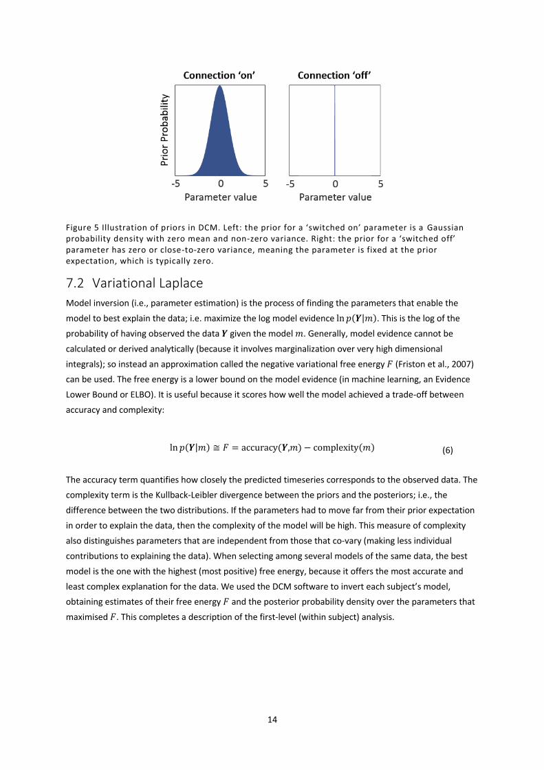
7.1 Priors

The priors over parameters in DCM form a multivariate normal density, which is specified by its mean and

covariance. Practically these densities are expressed as a vector of numbers (the mean or expected

values of the parameters) and a covariance matrix. Elements on the leading diagonal of the covariance

matrix are the prior variance (uncertainty) for each parameter, and the off-diagonal elements are the

covariance between the parameters. The choice of priors for each connectivity parameter depends on

whether the connection was ‘switched on’ or ‘switched off’. Each switched on parameter has expectation

zero and non-zero variance (Figure 5, left). This says that in the absence of evidence to the contrary, we

assume there is no connectivity or experimental effect, but we are willing to entertain positive or

negative values if the data support it. The width of this distribution (its variance) determines how

uncertain we are that the parameter is zero. The prior for each ‘switched off’ parameter has expectation

zero and variance close to zero (Figure 5, right). This says that we are certain that the parameter is zero,

regardless of the data. Both of these are called ‘shrinkage priors’, because, in the absence of evidence,

the posterior density shrinks to zero. For this experiment, we selected the connections to switch on and

off (Figure 3), and the DCM software translated these choices into priors for each parameter

(spm_dcm_fmri_priors.m). Note that by default, in order to decrease the time required for model

estimation, if more than eight brain regions are included then DCM automatically constrains the model

by using functional connectivity based sparsity-inducing priors (Seghier and Friston, 2013). This was not

the case here, and the priors for all free parameters are listed in Table 2.

14

Figure 5 Illustration of priors in DCM. Left: the prior for a ‘switched on’ parameter is a Gaussian probability density with zero mean and non-zero variance. Right: the prior for a ‘switched off’ parameter has zero or close-to-zero variance, meaning the parameter is fixed at the prior expectation, which is typically zero.

7.2 Variational Laplace

Model inversion (i.e., parameter estimation) is the process of finding the parameters that enable the

model to best explain the data; i.e. maximize the log model evidence ln 𝑝(𝒀|𝑚). This is the log of the

probability of having observed the data 𝒀 given the model 𝑚. Generally, model evidence cannot be

calculated or derived analytically (because it involves marginalization over very high dimensional

integrals); so instead an approximation called the negative variational free energy 𝐹 (Friston et al., 2007)

can be used. The free energy is a lower bound on the model evidence (in machine learning, an Evidence

Lower Bound or ELBO). It is useful because it scores how well the model achieved a trade-off between

accuracy and complexity:

ln 𝑝(𝒀|𝑚) ≅ 𝐹 = accuracy(𝒀,𝑚) − complexity(𝑚) (6)

The accuracy term quantifies how closely the predicted timeseries corresponds to the observed data. The

complexity term is the Kullback-Leibler divergence between the priors and the posteriors; i.e., the

difference between the two distributions. If the parameters had to move far from their prior expectation

in order to explain the data, then the complexity of the model will be high. This measure of complexity

also distinguishes parameters that are independent from those that co-vary (making less individual

contributions to explaining the data). When selecting among several models of the same data, the best

model is the one with the highest (most positive) free energy, because it offers the most accurate and

least complex explanation for the data. We used the DCM software to invert each subject’s model,

obtaining estimates of their free energy 𝐹 and the posterior probability density over the parameters that

maximised 𝐹. This completes a description of the first-level (within subject) analysis.

15

8 Results

8.1 Diagnostics

A basic diagnostic of the success of model inversion is to look at the estimated parameters and the

percentage variance explained by the model. Figure 6 (top) and Table 3 show the neural parameters from

a randomly selected subject (subject 37), which we will use to exemplify an interpretation of the

parameters (spm_dcm_review.m). Many of the neural parameters (𝑨,𝑩, 𝑪) moved away from their prior

expectation of zero, with 90% credible intervals (pink bars) that do not include zero. Figure 6 (bottom)

shows the modelled timeseries and residuals from this subject. There were clearly dynamics (solid lines)

related to the onsets of the task (grey boxes). The explained variance for this subject was 18.85% and the

mean across subjects was 17.27% (SD 9.37%), computed using spm_dcm_fmri_check.m. It is unsurprising

that the explained variance was quite low, because we did not model the control conditions (perceptual

matching) or the baseline rest periods. Nevertheless, most of the subjects evinced nontrivial neural

parameters, with 90% confidence intervals that excluded zero; so we could be confident that there was

useful information in the data pertaining to our experimental effects.

8.2 Interpretation of parameters

We will use the same subject’s model to interpret key parameters. The 𝑩 parameters are the most

interesting experimentally; these are the modulations of connections by each experimental condition

(Pictures and Words). Positive parameter estimates indicate increased self-inhibition due to the

experimental condition, and negative values meant disinhibition. We allowed picture and word stimuli to

modulate each of the self-connections, and three of these parameters, numbered 13, 14 and 17, deviated

with a high degree of posterior confidence from their prior expectation of zero. These are plotted in

Figure 6 (top) and are illustrated in green and red text in Figure 7. Picture stimuli increased self-inhibition

on ldF and decreased self-inhibition on lvF, thereby shifting responses from the dorsal to ventral frontal

cortex, specifically in the left hemisphere. Word stimuli increased self-inhibition in lvF, making it less

sensitive to input from the other modelled regions.

It is sufficient to report the estimated parameters and make qualitative statements about their meaning,

as above (e.g., that the strength of a particular connection was increased or decreased by an

experimental condition). However, what is the quantitative interpretation of these parameters? Taking

region lvF as an example, we can write out Equation 3 in full, to express the rate of change in lvF’s neural

activity. This is shown in Equation 7:

16

Figure 6 Example DCM neural parameters and model fit for a single subject. Top: The parameters corresponding to Equation 3. The error bars are 90% credible intervals , derived from the posterior variance of each parameter, and the vertical dotted lines distinguish different types of parameter . Note this plot does not show the covariance of the parameters, although this is estimated. The parameters are: the average inhibitory self-connections on each region across experimental conditions (𝑨𝑰), the average between-region extrinsic connections (𝑨𝑬), the modulation of

inhibitory self-connections by pictures (𝑩𝑰(2)) and by words (𝑩𝑰

(3)), and the driving inputs (𝑪). For a

full list of parameters, please see Table 3. Bottom: Example subject’s predicted timeseries (solid lines) with one line per brain region. The dotted lines show the model plus residuals. Underneath, blocks showing the timing of the word and picture trials.

17

��1 = (−0.5 ∙ exp(𝐴𝐼 11)⏟ Average

∙ exp (𝐵𝐼 11(2) ∙ 𝑢2(𝑡)) ∙⏟ Pictures

exp (𝐵𝐼 11(3) ∙ 𝑢3(𝑡))⏟ Words

)𝑧1

⏟ Self-connection

+𝐴𝐸 12 ∙ 𝑧2⏟ ldF→lvF (A)

+ 𝐴𝐸 13 ∙ 𝑧3⏟ rvF→lvF (A)

+ 𝐶11 ∙ 𝑢1(𝑡)⏟ Driving (C)

𝑢1(𝑡) = {0.6, 𝑡𝑎𝑠𝑘

−0.4, 𝑜𝑡ℎ𝑒𝑟𝑤𝑖𝑠𝑒

𝑢2(𝑡) = {0.8, 𝑝𝑖𝑐𝑡𝑢𝑟𝑒𝑠

−0.2, 𝑜𝑡ℎ𝑒𝑟𝑤𝑖𝑠𝑒

𝑢3(𝑡) = {0.8, 𝑤𝑜𝑟𝑑𝑠

−0.2, 𝑜𝑡ℎ𝑒𝑟𝑤𝑖𝑠𝑒

(7)

This says that the response in region lvF was governed by the strength of its self-connection (line 1 of

Equation 7) as well as incoming connections from regions ldF, rvF and the driving input (line 2 of Equation

7). The values for the experimental inputs 𝑢1(𝑡), 𝑢2(𝑡) and 𝑢3(𝑡) at time 𝑡 were set during the

specification of the model, due to mean-centring of the regressors (see Section 5.6: Centre input).

Plugging in the estimated parameters from Table 3, the self-inhibition in lvF during picture trials was

−0.5 ∙ exp(−0.16) ∙ exp(−0.47 ∙ 0.8) ∙ exp(2.8 ∙ −0.2) = − 0.17𝐻𝑧. The self-inhibition of lvF during

word trials was far stronger: −0.5 ∙ exp(−0.16) ∙ exp(−0.47 ∙ −0.2) ∙ exp(2.8 ∙ 0.8) = − 4.40𝐻𝑧 .

Therefore, region lvF was more sensitive to inputs from the rest of the network when the stimuli were

pictures than words. These task effects can also be expressed as a change in the time constant 𝜏 of region

lvF: 𝜏 = 5.88s in the context of pictures and 𝜏 = 0.23s in the context of words (see Appendix 4). Rewriting

this as the half-life of region lvF; neural activity decayed to half its starting level 4.08s after the onset of

picture stimuli and 0.16s after the onset of word stimuli. Picture stimuli therefore elicited a far more

sustained response in lvF than word stimuli. The other key factor influencing lvF was the incoming

connection from region rvF (0.43Hz), and the positive sign indicates this connection was excitatory.

Inspecting the parameters in this way provides insight into the sign and magnitude of the connection

strengths and experimental effects. However, this does not constitute a formal test of any hypotheses.

There are various strategies for testing hypotheses at the group (between-subject) level, using classical or

Bayesian statistics, and we detail these in the second part of the tutorial (please see the companion

paper).

18

Figure 7 Estimated parameters from a single subject. Between-region (extrinsic) parameters are in units of Hz, where positive numbers indicate excitation and negative numbers indicate inhibition. Self-connection parameters have no units and scale up or down the default self-connection of -0.5Hz (see Equation 3). Positive numbers for the self-connections indicate increased self-inhibition and negative numbers indicate disinhibition. For clarity, only parameters with 90% probability of being non-zero are displayed (see Table 3 for details) . Colours and line styles as for Figure 3.

9 Discussion This tutorial reviews the current implementation of DCM for fMRI by stepping through the analysis of a

factorial fMRI experiment. This first level (within-subject) analysis started by identifying brain regions

evincing experimental effects, for which we extracted representative fMRI timeseries. We then specified

a DCM, by selecting which connections should be ‘switched on’ and which should be ‘switched off’. This

specified the priors for the connectivity parameters. Inverting each subject’s model provided the strength

of connections (𝑨), the change in connections due to each experimental condition (𝑩) and the sensitivity

of each region to external input (𝑪), as well as the free energy approximation to the log model evidence

𝐹. The appendices provide the technical detail of each of these steps.

A common question from users is: what assumptions are made by DCM? As a Bayesian model, most

assumptions are stated up-front as priors. The key assumptions for the basic (deterministic 1-state

bilinear) neural model are as follows:

The pre-processed fMRI timeseries used for DCM have been selected because they show

experimental effects. The signals are averaged over voxels and nuisance effects are regressed

out, therefore, the signal-to-noise ratio is high – the prior expectation of the variance of the

noise is 1

exp(6)= 0.0025 (see Appendix 2). This expresses the prior belief that most of the

variance is interesting and where possible, we would like the variance to be ascribed to the

model rather than to observation noise. Furthermore, the variance of the observation noise is

assumed to be independent of the neural / haemodynamic parameters.

The neural response due to intrinsic (within-region) activity is expected to decay over a period of

seconds following experimental stimulation. The prior on the self-connection parameters says

that an isolated brain region’s time constant τ will be between 1.63s and 2.46s with 90%

19

probability, and between 0.38s and 10.49s in the context of modulation by an experimental

condition (Appendix 4). This response will be further added to or subtracted from by incoming

connections from other regions.

The priors for the parameters of the haemodynamic, BOLD signal and observation models are

consistent with empirical measurements using animal models and human subjects (c.f. Buxton et

al., 1998; Stephan et al., 2007). In DCM for fMRI, three of these parameters are estimated from

the data and the priors are listed in Table 2. Values for fixed parameters, which are not

estimated from the data, can be found in the Matlab functions spm_fx_fmri.m and

spm_gx_fmri.m.

The free energy is assumed to serve as a good proxy for the log model evidence. This is exactly

true for linear models (where the free energy becomes log model evidence) and has been

validated for weakly non-linear models like DCM for fMRI using sampling methods (Chumbley et

al., 2007). Caution needs to be taken with highly nonlinear models, where local optima pose a

challenge; one method for addressing this is to use a multi-start estimation algorithm which re-

initializes subject-level inversions using group-level estimated parameters (Friston et al., 2015).

The next step in our analysis was to test which neural effects were conserved over subjects, and which

differed due to brain Laterality Index – the between-subjects factor that was the focus of this experiment.

These analyses are detailed in the companion paper, where we cover Bayesian model comparison (i.e.,

hypothesis testing) at the within and between subject level.

10 Appendix 1: Timeseries extraction Before a DCM can be specified, Regions of Interest (ROIs) need to be selected and representative

timeseries extracted from each. The fMRI data for a subject can be considered a large 4D matrix �� where

the first three dimensions are space and the fourth dimension is time (in scans). By extracting timeseries,

we seek to reduce this to a smaller matrix 𝒀 where there are a small number of ROIs that define our brain

network. There are various strategies for selecting the voxels that contribute to each ROI – indeed,

questions pertaining to this are among the most common from DCM users on the SPM Mailing List. The

most important consideration is that DCM is intended to explain the coupling between neural

populations that show experimental effects. An initial GLM analysis is therefore normally used to identify

voxels that show a response to each experimental factor. To reduce noise, only voxels that exceed some

liberal statistical threshold for a contrast of interest are usually retained.

For the data presented here, the following steps were applied by (Seghier et al., 2011), which may

provide a useful recipe for preparing DCM studies:

1. Statistical Parametric Mapping (SPM). A General Linear Model (GLM) was specified for each

subject, and T-contrasts were computed to identify brain regions that showed a main effect of

each factor and an interaction between factors. Additionally, an F-contrast was calculated to

identify all ‘Effects of Interest’ – to later regress out any uninteresting effects such as head

20

motion or breathing from the timeseries. This F-contrast was an identity matrix of dimension 𝑛,

where the first 𝑛 columns in the design matrix related to interesting experimental effects.

2. Group-level region selection. Contrast maps from each subject were summarized at the group

level using one-sample t-tests. These group-level results were used to select the peak MNI

coordinates of the ROIs. Different contrasts could have been used to select each ROI; however,

in this case, the main effect of task (semantic > perceptual matching) was used to identify all

four ROIs.

3. Subject-level feature selection. Having identified the ROI peak coordinates at the group level,

the closest peak coordinates for each individual subject were identified. This allowed for each

subject to have slightly different loci of responses. Typically, one would constrain each subject-

level peak to be within a certain radius of the group-level peak, or alternatively, to be within the

same anatomical structure (e.g. using an anatomical mask). Here, subject-level peaks were

constrained to be a maximum of 8mm from the group level peak, and had to exceed a liberal

statistical threshold of p < 0.05 uncorrected.

At this stage, Seghier et al. (2011) excluded any subjects not showing experimental effects in

every brain region above the statistical threshold. We suggest that with the development of

hierarchical modelling of connectivity parameters, detailed in the second part of this tutorial,

removing subjects with noisy or missing data in certain brain regions may be unnecessary. A

subject who lacks a strong response in one brain region or experimental condition, for whatever

reason, may still contribute useful information about other brain regions or conditions (and

indeed useful information about intersubject variability). Therefore, when an ROI contains no

voxels showing a response above the selected threshold, we recommend dropping the

threshold until a peak voxel coordinate can be identified.

4. ROI definition. Having identified the peak coordinates for each ROI, timeseries were extracted.

Each ROI was defined as including all the voxels which met two criteria: 1) located within a

sphere centred on the individual subject’s peak with 4mm radius and 2) exceeded a threshold of

p < 0.05 uncorrected, for the task contrast at the single-subject level. Note that applying a

threshold at this stage is not to ensure statistical significance (this happens in step 2). Rather,

the threshold is simply used to exclude the noisiest voxels from the analysis.

5. ROI extraction. SPM was used to extract representative timeseries from each ROI, which

invoked a standard series of processing steps (spm_regions.m). The timeseries are pre-whitened

21

(to reduce serial correlations), high-pass filtered, and any nuisance effects not covered by the

Effects of Interest F-contrast are regressed out of the timeseries (i.e. ‘adjusted’ to the F-

contrast). Finally, a single representative timeseries is computed for each ROI by performing a

principal components analysis (PCA) across voxels and retaining the first component (or

principal eigenvariate). This approach is used rather than taking the mean of the timeseries,

because calculating the mean would cause positive and negative responses to cancel out (and

further that means are effected by extreme values). That could pose a problem due to centre-

surround coding in the brain, where excitatory responses are surrounded by inhibitory

responses – and would cancel if averaged.

Additionally, prior to DCM model estimation, the software automatically checks whether the fMRI data

are within the expected range (spm_dcm_estimate.m). If the range of the fMRI data exceeds four (in the

units of the data), DCM rescales the data to have a range of four, on a per-subject basis. This was the case

for our data.

These steps produced one timeseries per region, for each subject, which were then entered into the DCM

analysis. The complete pipeline above can be performed in the SPM software semi-automatically, using

the steps described in the practical guide.

11 Appendix 2: Observation noise specification DCM separately estimates the precision (inverse variance) of zero-mean additive white noise for each

brain region (spm_nlsi_gn.m). The white noise assumption is used because the preliminary general linear

model estimates serial correlations, which are used to whiten principal eigenvariates from each region.

From Equation 1 we have the model:

𝒀 = 𝑔(𝒛, 𝜽(𝒉)) + 𝑿𝟎𝚩𝟎 + 𝝐 (8)

To simplify the implementation, 𝒀 is vectorised (the timeseries from each region are stacked on top of

one another) to give 𝒚𝒗 = 𝑣𝑒𝑐(𝒀). The observation noise 𝝐 is specified according to a normal density:

𝝐~𝑁(𝟎, 𝚺𝒚) (9)

In practice, DCM uses the precision matrix 𝚷𝒚 which is the inverse of the covariance matrix 𝚺𝒚. It is

specified by a multi-component model, which is a linear mixture of precision components 𝑸𝒊 with one

component per brain region 𝑖 = 1…𝑅. Each precision matrix is weighted by a parameter 𝜆𝑖 which is

estimated from the data:

22

𝚷𝒚 =∑exp(𝜆𝑖)𝑸𝒊𝑖

(10)

The diagonal elements of the precision matrix 𝑸𝒊 have value one for observations associated with brain

region 𝑖 and zero elsewhere. Taking the exponential of parameter 𝜆𝑖 ensures that the estimated precision

cannot be negative. In total, in the experiment presented here, we had 792 observations per subject (𝑇 =

198 fMRI volumes times 𝑅 = 4 brain regions), and the corresponding precision components are

illustrated in Figure A.1.

From Table 2, the prior density for parameter 𝜆𝑖 was 𝑁 (6,1

128). This means that scaling factor exp(𝜆𝑖)

had a lognormal prior density: 𝐿𝑜𝑔𝑛𝑜𝑟𝑚𝑎𝑙 (6,1

128). The resulting prior expected precision was exp(6) =

403.43 with 90% credible interval [348.84 466.56]. This prior says that the data were expected to have a

high signal-to-noise ratio, because the fMRI data were highly pre-processed and averaged, and are

selected from brain regions that are known to show experimental effects. Model inversions are therefore

preferred which ascribe a high level of variance to the model rather than to noise.

Figure A.1 Illustration of the observation noise model in DCM for fMRI. Each precision component 𝑸 was a matrix with 𝑇 ∙ 𝑅 = 792 elements, and there was one precision component per brain region. Log scaling parameter 𝜆𝑖 was estimated from the data and scaled up or down the corresponding component 𝑸𝒊.

12 Appendix 3: Derivation of the fMRI neural model Neural responses may be written generically as follows:

�� =𝒅𝒛

𝑑𝑡= 𝑓(𝒛, 𝒖) (11)

Where vector 𝒛 is the state or level of activity in each region, �� is the rate of change in each brain region –

called the neural response - and 𝑓 is a function describing the change in brain activity in response to

experimental inputs 𝒖. The ‘true’ function 𝑓 would be tremendously complicated, involving the

nonlinear, complex and high dimensional dynamics of all cell types involved in generating a neural

response. Instead, we can approximate 𝑓 using a simple mathematical tool – a Taylor series. The more

terms we include in this series, the closer we get to reproducing the true neural response. The definition

of the Taylor series 𝑇 up to the second term, with two variables 𝑧 and 𝑢 evaluated at 𝑧 = 𝑚 and 𝑢 = 𝑛 is:

23

𝑇(𝑧, 𝑢) = 𝑓(𝑚, 𝑛)

+(𝑧 −𝑚) ∙ 𝑓𝑧

+(𝑢 − 𝑛) ∙ 𝑓𝑢

+1

2((𝑧 − 𝑚)2 ∙ 𝑓𝑧𝑧 + 2(𝑧 −𝑚)(𝑢 − 𝑛) ∙ 𝑓𝑧𝑢 + (𝑢 − 𝑛)

2 ∙ 𝑓𝑢𝑢)

(12)

Where 𝑓𝑧 and 𝑓𝑢 are the partial derivatives of 𝑓 with respect to 𝑧 and 𝑢, 𝑓𝑧𝑧 and 𝑓𝑢𝑢 are the second order

derivatives and 𝑓𝑧𝑢 is the mixed derivative (i.e. the derivative of 𝑓 with respect to 𝑧 of the derivative with

respect to 𝑢, or vice versa). Each of these partial derivatives is evaluated at (𝑧 = 𝑚, 𝑢 = 𝑛). Setting 𝑚 =

0 and 𝑛 = 0, defining the baseline neural response 𝑓(𝑚, 𝑛) = 0 and dropping the higher order terms we

get the simpler expression:

𝑇(𝑧, 𝑢) = 0 +𝑧 ∙ 𝑓𝑧 +𝑢 ∙ 𝑓𝑢

+1

2(𝑧2 ∙ 𝑓𝑧𝑧 + 2𝑧𝑢 ∙ 𝑓𝑧𝑢 + 𝑢

2 ∙ 𝑓𝑢𝑢)

(13)

By re-arrangement of the final term:

𝑇(𝑧, 𝑢) = 𝑧 ∙ 𝑓𝑧 +𝑢 ∙ 𝑓𝑢 +𝑧𝑢 ∙ 𝑓𝑧𝑢

+1

2(𝑧2 ∙ 𝑓𝑧𝑧 + 𝑢

2 ∙ 𝑓𝑢𝑢)

(14)

Finally, factorizing 𝑧 and dropping the final term (as 𝑧2 and 𝑢2 will be very small around the origin) gives:

𝑇(𝑧, 𝑢) = (𝑓𝑧 + 𝑢 ∙ 𝑓𝑧𝑢)𝑧 + 𝑢 ∙ 𝑓𝑢

= (𝐴 + 𝐵𝑢)𝑧 + 𝐶𝑢 (15)

Here, we have assigned letters to the three derivative terms 𝐴 = 𝑓𝑧, 𝐵 = 𝑓𝑧𝑢, 𝐶 = 𝑓𝑢, which gives the

expression for the neural model used in in the DCM literature (Equation 2). With multiple brain regions,

these becomes matrices. As introduced in the main text, 𝑨 is the rate of change in neural response due to

the other neural responses in the system – i.e. the effective connectivity. 𝑩 is the rate of change in

effective connectivity due to the inputs and is referred to as the bilinear or interaction term. Finally, 𝑪 is

the rate of change in neural response due to the external input, referred to as the driving input. In the

DCM framework, 𝑨, 𝑩 and 𝑪 become parameters which are estimated from the data. (To apply negativity

constraints on the self-connections, 𝑨 and 𝑩 are sub-divided into intrinsic and extrinsic parts, see

Equation 3.)

13 Appendix 4: The neural parameters Whereas Appendix 3 motivated the DCM neural model as a function approximated by a Taylor series,

here we consider it from the perspective of a simple dynamical system, to help gain an intuition for the

24

parameters. Consider a DCM with a single brain region, driven by a brief stimulus at time 𝑡 = 0. The

neural equation can be simplified to the following:

�� = 𝑎𝑧 (16)

Where self-connection or rate constant 𝑎 has units of Hz and is negative. The solution to this equation,

the neural activity at any given time, is an exponential decay (under the constraint that 𝑎 is negative):

𝑧(𝑡) = 𝑧(0) ∙ exp(𝑎𝑡) (17)

Where 𝑧(0) is the initial neuronal activity. This function is plotted in Figure A.2 (left) with parameter =

−0.5𝐻𝑧 , which is the default value in DCM.

Figure A.2 Illustration of neural response as an exponential decay. Left: the neural response under the default prior of a = -0.5Hz to an instantaneous input at time zero. Also plotted are the corresponding time constant 𝜏 and half-life. Middle: The resulting prior over time constant 𝜏 in the absence of modulation. The median is 𝜏 = 2 seconds with 90% credible interval [1.63s 2.46s]. Right: The prior over 𝜏 in the presence of modulation. The median is 𝜏 = 2 seconds with 90% credible interval [0.38s 10.49s]. Green dashed lines in the middle and right panels show the median.

Figure A.2 (left) also illustrates two common ways of characterizing the rate of decay. The time constant 𝜏

is defined as:

𝜏 = −1

𝑎 (18)

This is the time in seconds taken for the neural activity to decay by a factor of 1

𝑒 (36.8% of its peak

response). Given 𝑎 = −0.5𝐻𝑧 the time constant is 𝜏 = 2s. This inverse relationship between the rate

constant 𝑎 and time constant 𝜏 is why the connectivity parameters in DCM are in units of 𝐻𝑧 (𝐻𝑧 is

1/seconds). It can be more intuitive to express the rate of decay as the half-life, which is the time at

which the activity decays to half its starting value. Given the self-connection of -0.5Hz, the half-life is:

25

𝑡12= 𝜏 ∙ ln 2 = 1.39s (19)

In DCM we specify a prior probability density over each self-connection parameter 𝑎, which in turn

specifies our expectation about a typical region’s time constant. Figure A.2 (centre) shows the resulting

prior time constant in DCM for fMRI. The median is 2s with 90% of the probability mass (the credible

interval) between 1.63s and 2.46s.

In our analyses, we allowed self-connections to be modulated by experimental conditions. The rate

constant 𝑎 was therefore supplemented to give 𝑎 + 𝑏 ∙ 𝑢 (see Equation 2 of the main text). The

modulatory parameter 𝑏, multiplied by the experimental input 𝑢, could increase or decrease the region’s

rate of decay. Figure A.2 (right) shows the prior time constant for connections with modulation switched

on (where 𝑢 = 1), giving 90% credible interval [0.38s 10.49s]. These plots make clear that DCM for fMRI

does not model the activity of individual neurons, which typically have time constants on the order of

milliseconds. Rather, it models the slow emergent dynamics that evolve over seconds and arise from the

interaction of populations of neurons. For details of how these plots were generated, please see the

supplementary text.

14 Appendix 5: Haemodynamic and BOLD signal model The translation of neural activity 𝑧, predicted by the DCM neural model, to observed BOLD response 𝑦, is

described by a three-part model illustrated in Figure A.2. We will summarise each of the three parts in

turn.

Figure A.2 The model used to translate from neural activity to the BOLD signal in DCM. This is split into three parts. i. Neural activity 𝑧(𝑡) triggers a vasoactive signal 𝑠 (such as nitric oxide) which in turn causes an increase in blood flow. ii. The flow inflates the blood vessel like a balloon, causing a change in both blood volume 𝑣 and deoxyhaemoglobin (dHB) 𝑞. iii. These combine non-linearly to give rise to the observed BOLD signal. A key reference for each part of the model is given - see text for further details. Symbols outside the boxes are parameters and those in bold type are free parameters that are estimated from the data: decay 𝜅, transit time 𝜏ℎ and ratio of intravascular to

26

extravascular contribution to the signal 𝜖ℎ. See Table 1 for a full list of symbols. Adapted from Friston et al. (2000).

14.1 Regional cerebral blood flow (rCBF)

Neural activity 𝑧(𝑡) drives the production of a chemical signal 𝑠 that dilates local blood vessels. This

causes oxygenated blood to flow into the capillaries, where oxygen is extracted. As a result, partially

deoxygenated blood flows into the veins (venous compartment). The vasodilatory signal 𝑠 decays

exponentially and is subject to feedback by the blood flow 𝑓𝑖𝑛 that it induces:

��𝑖𝑛 = 𝑠

�� = 𝑧(𝑡) − 𝜅𝑠 − 𝛾(𝑓𝑖𝑛 − 1) (20)

Where parameter 𝜅 is the rate of decay for the signal 𝑠, and 𝛾 is the time constant controlling the

feedback from blood flow. Empirical estimates have shown 𝜅 to have a half-life of around one second

(Friston et al., 2000), placing it in the correct range to be mediated by nitric oxide (NO). Adjusting 𝜅

primarily changes the peak height of the modelled BOLD response, whereas adjusting 𝛾 primarily changes

the duration of response. Both parameters also modulate the size of the post-stimulus undershoot.

14.2 Venous balloon

Increased blood flow causes a local change in the volume of blood 𝑣 in the blood vessel, as well as the

proportion of deoxyhaemoglobin 𝑞 (dHb). This process is captured by the Balloon model of Buxton et al.

(1998). It treats the venous compartment as a balloon, which inflates due to increased blood flow and

consequently expels deoxygenated blood at a greater rate. The change in blood volume 𝑣, normalized to

the value at rest, depends on the difference blood inflow and outflow:

𝜏ℎ�� = 𝑓𝑖𝑛(𝑡) − 𝑓𝑜𝑢𝑡(𝑣, 𝑡)

𝑓𝑜𝑢𝑡(𝑣, 𝑡) = 𝑣(𝑡)1𝛼

(21)

Where the time constant 𝜏ℎ is the mean transit time of blood, i.e. the average time it takes for blood to

traverse the venous compartment. Grubb’s parameter 𝛼 controls the stiffness of the blood vessel (Grubb

et al., 1974) and adjusting it has the effect of changing the peak height of the modelled BOLD response.

The increase in blood volume following neural activity is accompanied by an overall decrease in dHb, the

rate of which depends on the delivery of dHb into the venous compartment minus the amount expelled:

𝜏ℎ�� = 𝑓𝑖𝑛(𝑡)1 − (1 − 𝐸0)

1𝑓𝑖𝑛

𝐸0−𝑓𝑜𝑢𝑡(𝑣, 𝑡)(𝑞(𝑡))

𝑣(𝑡) (22)

The first expression on the right hand side of Equation 22 approximates the fraction of oxygen extracted

from the inflowing blood, which depends on the inflow 𝑓𝑖𝑛 and the resting oxygen extraction fraction 𝐸0

(the percentage of the oxygen removed from the blood by tissue during its passage through the capillary

network). The second term relates to the outflow, where the ratio 𝑞/𝑣 is the dHb concentration.

27

14.3 BOLD signal

Finally, the change in blood volume 𝑣 and dHb 𝑞 combine to cause the BOLD signal 𝑆, measured using

fMRI. For the purpose of this paper we define 𝑆 as the signal acquired using a gradient echo EPI readout.

The model used in DCM is due to Buxton et al. (1998) and Obata et al. (2004), which were extended and

re-parameterised by Stephan et al. (2007). In the following paragraphs we provide a recap of the basic

mechanisms of MRI and functional MRI (fMRI), in order to motivate the form of the BOLD signal model.

Readers familiar with MR physics may wish to skip this introduction.

We will use classical mechanics to describe the way the MR signal is generated. When entering an MRI

scanner, the subject is exposed to the main magnetic field 𝒃𝟎. This magnetic field is always on and its axis

is aligned with the tunnel of the scanner. All the hydrogen protons of the body can be thought of as acting

like tiny magnets whose strength is measured by their magnetic moments 𝛍. In what follows, the

coordinate system x,y,z is used where z corresponds to the 𝒃𝟎 axis, y and x are the orthogonal vectors

forming the transverse plane. When submitted to the magnetic field B0, two phenomena occur:

1/ All of the proton magnetic moments precess about the 𝒃𝟎 axis at the Larmor frequency, which is

proportional to the amplitude of the 𝒃𝟎 field strength (e.g. 123MHz at 3T).

2/ The proton magnetic moments orient themselves such that their vector sum is a net magnetization

vector, 𝒎, aligned with the 𝒃𝟎 field axis and pointing in the same direction (Figure A.3.i). The net

magnetization vector 𝒎 can be decomposed into two components, the longitudinal component 𝒎𝒛 along

the z axis and the transverse component 𝒎𝒙𝒚, which is the projection of 𝒎 into the transverse plane. The

transverse component is zero when the system is at equilibrium; i.e., when the net magnetization is aligned

with the z axis, yet it is only the transverse component that can be measured in MRI.

In order to disturb the equilibrium state and thereby create a transverse component 𝒎𝒙𝒚 that can be

detected, a rotating magnetic field 𝒃𝟏 is applied orthogonal to the 𝒃𝟎 axis for a short period of time. This

is termed ‘excitation’ and results in the tilting of the net magnetization towards the transverse plane (Figure

A.3.ii).

Once the 𝒃𝟏 field is turned off, the net magnetization has a transverse component and continues to precess

around the main magnetic field, 𝒃𝟎. Since the precession frequency is proportional to the amplitude of the

magnetic field, any spatial variation of the magnetic field amplitude across one voxel will induce a

difference in precessional frequency for the protons. For this reason, the protons accumulate a delay

relative to each other and so have differential phase (orientation, Figure A.3.iii). Over time the delays, or

relative phase difference, increase (Figure A.3.iv). As a result their vector sum; i.e., the transverse

component 𝒎𝒙𝒚 decreases. This process, whereby the transverse component of the net magnetisation

decreases, is called effective transverse relaxation. It is characterized by an exponential decay with a time

constant 𝑇2∗ (Figure A.3.v), or alternatively a relaxation rate 𝑅2

∗, whereby 𝑅2∗ =

1

𝑇2∗.

Crucially, for functional MRI, dhB and oxyhaemoglobin (Hb) molecules have different magnetic

susceptibility (i.e. a different response to being placed in a magnetic field). Unlike Hb, which exhibits a

weak, diamagnetic response to the main magnetic field, dHb exhibits a stronger, paramagnetic response.

At the boundaries between two tissues with different magnetic susceptibilities, the magnetic field is

28

distorted, increasing the local spatial inhomogeneity in the amplitude of the magnetic field. The decrease

in dHb following neural activity makes the blood less paramagnetic, and more similar to the surrounding

tissue in terms of magnetic susceptibility. As a result, the magnetic field around the blood vessel becomes

less distorted, with a smaller range of precessional frequencies of protons in the voxel. As a consequence,

less differential phase accumulates between the proton magnetic moments and the amplitude of the

transverse component of the net magnetization vector 𝒎𝒙𝒚 decreases less rapidly. This corresponds to a

shorter 𝑅2∗ (or equivalently a longer 𝑇2

∗). Therefore, at the time the data are acquired, TE (Echo Time), the

signal will be higher if it follows a period of neural activity.

Figure A.3 Generation of the Magnetic Resonance (MR) signal. i. When exposed to a strong magnetic field, proton magnetic moments 𝛍 add together to create a net magnetization 𝒎, aligned

29

with the B0 axis pointing in the same direction as this main field. ii After excitation with a flip angle (𝛼) imparted by a rotating B1 field applied orthogonal to B0 for a short period of time, the net magnetization is composed of a longitudinal and a transverse component, which precesses about the B0 axis. iii Inhomogeneity in the magnetic field within a voxel causes the protons’ magnetic moments to precess with different frequency leading to differential phase (orientation) between the protons, reducing the transverse component 𝐦𝐱𝐲 which is the vector sum of all the protons. iv.

The differential phase accumulated by the protons increases over time. v. As a result, the amplitude of the transverse component of the net magnetization (i.e. the detectable MR signal) further decreases, following an exponential decay characterized by the effective transverse relaxation rate R2*=1/T2*. The MR signal is acquired at an echo time TE. vi. DCM assumes that there are two contributions to the measured signal – intravascular (𝑆𝑖) and extravascular (𝑆𝑒) – each with their own 𝑅2

∗ relaxation rates.

Having revised the fundamentals of fMRI, we now return to the BOLD signal model in DCM. It follows

Ogawa et al. (1993), in treating the tissue within a voxel as consisting of many small cubes, each with a

cylinder running through the centre (Figure A.3vi). There are two compartments – the extravascular tissue

outside the cylinder and the blood vessel (intravascular venous compartment) that is filled with blood. The

BOLD signal at rest 𝑆0 is modelled as a linear mixture of these extravascular and intravascular contributions

(Buxton et al., 1998):

𝑆0 = (1 − 𝑉0)𝑆𝑒 + 𝑉0𝑆𝑖 (23)

Where 𝑉0 is the fraction of the BOLD signal originating from the intravascular compartment. From Obata

et al. (2004), each compartment’s resting BOLD signal at the time of measurement, 𝑇𝐸 in seconds, is

modelled by:

𝑆𝑒 = 𝑆𝑒0 ∙ exp(−𝑅2𝑒

∗ ∙ 𝑇𝐸) 𝑆𝑖 = 𝑆𝑖0 ∙ exp(−𝑅2𝑖

∗ ∙ 𝑇𝐸) (24)

Where 𝑅2𝑒∗ and 𝑅2𝑖

∗ are the effective transverse relaxation rates for the extravascular and intravascular

compartments respectively, in units of Hz, and 𝑆𝑒0 and 𝑆𝑖0 are the maximal signals originating from each

compartment before any signal decrease due to differential dephasing of the protons. Following neural

activation, there will be an altered BOLD signal, 𝑆, compared to 𝑆0, written Δ𝑆 = 𝑆 − 𝑆0. A linear

approximation of this change is as follows:

Δ𝑆

𝑆0≈ −(Δ𝑅2𝑒

∗ ∙ 𝑇𝐸) − (𝑉0 ∙ 𝜖ℎ ∙ Δ𝑅2𝑖∗ ∙ 𝑇𝐸) + (𝑉0 − 𝑉1)(1 − 𝜖ℎ) (25)

Where Δ𝑅2𝑒∗ and Δ𝑅2𝑖

∗ is the change in each compartment’s 𝑅2∗ between activation and rest, 𝜖ℎ =

𝑆𝑖

𝑆𝑒 is the

ratio of intra- to extra-vascular signal contributions and 𝑉1 is the volume of venous blood following

activation (Obata et al., 2004; Stephan et al., 2007). Obata et al. (2004) derived approximations for the

changes in extravascular and intravascular signal decay:

30

Δ𝑅2𝑒∗ = 4.3 ∙ 𝜗0 ∙ 𝑉0 ∙ 𝐸0 ∙ (𝑞 − 1)

Δ𝑅2𝑖∗ = 𝑟0 ∙ 𝐸0 ∙ (

𝑞

𝑣− 1)

(26)

Where ϑ0 is the frequency offset at the outer surface of magnetised vessels in units of Hz, 𝐸0 is the fraction

of oxygen extraction at rest, and 𝑟0 is a constant relating Δ𝑅2𝑖∗ to the oxygen extraction rate. Plugging these

into Equation 25 and re-arranging gives the final expression (Stephan et al., 2007):

Δ𝑆

𝑆0≈ 𝑉0 (𝑘1(1 − 𝑞) + 𝑘2 (1 −

𝑞

𝑣) + 𝑘3(1 − 𝑣))

𝑘1 = 4.3 ∙ 𝜗0 ∙ 𝐸0 ∙ 𝑇𝐸

𝑘2 = 𝜖ℎ ∙ 𝑟0 ∙ 𝐸0 ∙ 𝑇𝐸

𝑘3 = 1 − 𝜖ℎ

(27)

The three terms inside the brackets, weighted by coefficients 𝑘1, 𝑘2 and 𝑘3, relate to the extravascular

contribution to the BOLD signal, the intravascular contribution and the ratio of extravascular and

intravascular signals respectively.

14.4 Summary and implementation

The implementation of haemodynamic model in SPM is split into two parts: the rCBF / Balloon model

(spm_fx_fmri.m) and the BOLD signal model (spm_gx_fmri.m). They include five hidden states: the net

neural activity 𝑧, vasoactive signal 𝑆, log rCBF ln(𝑓𝑖𝑛), log venous volume ln(𝑣) and log dHb ln(𝑞). The

logs of these states are taken in order to enforce positivity constraints, requiring the differential

equations to be supplemented accordingly:

𝑑 ln(𝑓𝑖𝑛)

𝑑𝑡=��𝑖𝑛𝑓𝑖𝑛

𝑑 ln(𝑣)

𝑑𝑡=��

𝑣

𝑑 ln(𝑞)

𝑑𝑡=𝑞

𝑞

(28)

There are 10 parameters overall, labelled in Figure A.2. To keep estimation of the model tractable, only

three of these are estimated from the fMRI data, and the log of their values are estimated to ensure

positivity: the rate of signal decay ln(𝜅) from the rCBF model, the transit time ln(𝜏ℎ) from the balloon

model, and the ratio of intra- to extra-vascular signals ln(𝜖ℎ) from the BOLD signal model. The priors for

these parameters are listed in Table 2.

31

15 References Bastos AM, Usrey WM, Adams RA, Mangun GR, Fries P, Friston KJ (2012) Canonical microcircuits for predictive

coding. Neuron 76:695-711. Buxton RB, Wong EC, Frank LR (1998) Dynamics of blood flow and oxygenation changes during brain activation:

the balloon model. Magnetic resonance in medicine : official journal of the Society of Magnetic Resonance in Medicine / Society of Magnetic Resonance in Medicine 39:855-864.

Chumbley JR, Friston KJ, Fearn T, Kiebel SJ (2007) A Metropolis-Hastings algorithm for dynamic causal models. NeuroImage 38:478-487.

Deco G, Jirsa VK, Robinson PA, Breakspear M, Friston K (2008) The dynamic brain: from spiking neurons to neural masses and cortical fields. PLoS computational biology 4:e1000092.

Friston K, Zeidman P, Litvak V (2015) Empirical Bayes for DCM: A Group Inversion Scheme. Front Syst Neurosci 9:164.

Friston K, Mattout J, Trujillo-Barreto N, Ashburner J, Penny W (2007) Variational free energy and the Laplace approximation. NeuroImage 34:220-234.

Friston KJ, Harrison L, Penny W (2003) Dynamic causal modelling. NeuroImage 19:1273-1302. Friston KJ, Mechelli A, Turner R, Price CJ (2000) Nonlinear responses in fMRI: the Balloon model, Volterra

kernels, and other hemodynamics. NeuroImage 12:466-477. Friston KJ, Kahan J, Biswal B, Razi A (2014) A DCM for resting state fMRI. NeuroImage 94:396-407. Grubb RL, Raichle ME, Eichling JO, Ter-Pogossian MM (1974) The effects of changes in PaCO2 cerebral blood

volume, blood flow, and vascular mean transit time. Stroke 5:630-639. Kahan J, Foltynie T (2013) Understanding DCM: ten simple rules for the clinician. NeuroImage 83:542-549. Kahan J, Urner M, Moran R, Flandin G, Marreiros A, Mancini L, White M, Thornton J, Yousry T, Zrinzo L (2014)

Resting state functional MRI in Parkinson’s disease: the impact of deep brain stimulation on ‘effective’connectivity. Brain : a journal of neurology 137:1130-1144.

Kiebel SJ, Kloppel S, Weiskopf N, Friston KJ (2007) Dynamic causal modeling: a generative model of slice timing in fMRI. NeuroImage 34:1487-1496.

Li B, Daunizeau J, Stephan KE, Penny W, Hu D, Friston K (2011) Generalised filtering and stochastic DCM for fMRI. NeuroImage 58:442-457.

Marreiros AC, Kiebel SJ, Friston KJ (2008) Dynamic causal modelling for fMRI: a two-state model. NeuroImage 39:269-278.

Moran R, Pinotsis DA, Friston K (2013) Neural masses and fields in dynamic causal modeling. Front Comput Neurosci 7:57.

Obata T, Liu TT, Miller KL, Luh W-M, Wong EC, Frank LR, Buxton RB (2004) Discrepancies between BOLD and flow dynamics in primary and supplementary motor areas: application of the balloon model to the interpretation of BOLD transients. NeuroImage 21:144-153.

Ogawa S, Menon RS, Tank DW, Kim SG, Merkle H, Ellermann JM, Ugurbil K (1993) Functional brain mapping by blood oxygenation level-dependent contrast magnetic resonance imaging. A comparison of signal characteristics with a biophysical model. Biophys J 64:803-812.

Papadopoulou M, Cooray G, Rosch R, Moran R, Marinazzo D, Friston K (2017) Dynamic causal modelling of seizure activity in a rat model. NeuroImage 146:518-532.

Razi A, Kahan J, Rees G, Friston KJ (2015) Construct validation of a DCM for resting state fMRI. NeuroImage 106:1-14.

Rosch RE, Hunter P, Baldeweg T, Friston K, Meyer M (2017) Imaging and dynamic causal modelling reveal brain-wide changes in effective connectivity and synaptic dynamics during epileptic seizures. bioRxiv [PREPRINT].

Seghier ML, Friston KJ (2013) Network discovery with large DCMs. NeuroImage 68:181-191. Seghier ML, Josse G, Leff AP, Price CJ (2011) Lateralization is predicted by reduced coupling from the left to

right prefrontal cortex during semantic decisions on written words. Cerebral cortex 21:1519-1531. Seghier ML, Zeidman P, Neufeld NH, Leff AP, Price CJ (2010) Identifying abnormal connectivity in patients using

dynamic causal modeling of FMRI responses. Front Syst Neurosci 4. Stephan KE (2004) On the role of general system theory for functional neuroimaging. J Anat 205:443-470. Stephan KE, Weiskopf N, Drysdale PM, Robinson PA, Friston KJ (2007) Comparing hemodynamic models with

DCM. NeuroImage 38:387-401. Stephan KE, Penny WD, Moran RJ, den Ouden HE, Daunizeau J, Friston KJ (2010) Ten simple rules for dynamic

causal modeling. NeuroImage 49:3099-3109.

32

Stephan KE, Kasper L, Harrison LM, Daunizeau J, den Ouden HE, Breakspear M, Friston KJ (2008) Nonlinear dynamic causal models for fMRI. NeuroImage 42:649-662.

33

16 Tables

16.1 Table 1: Symbols

Variable Dimension Units Meaning

𝐴 𝑅 × 𝑅 Hz Effective connectivity (average or baseline)

𝐴𝐸 𝑅 × 𝑅 Hzs Extrinsic average or baseline effective connectivity

𝐴𝐼 𝑅 × 𝑅 - Log scaling parameters on average or baseline intrinsic connections

𝛼 1 × 1 - Grubb’s exponent (stiffness of blood vessels)

𝐵(𝑘) 𝑅 × 𝑅 Hz Modulatory input parameters for condition 𝑘

𝐵𝐸(𝑘)

𝑅 × 𝑅 Hz Modulation of extrinsic connections by condition 𝑘

𝐵𝐼(𝑘)

𝑅 × 𝑅 - Log scaling parameters on modulation of intrinsic connections by condition 𝑘

Β0 𝐶0 × 𝑅 - Parameters for null effects

𝐶 𝑅 × 𝐽 Hz Driving input parameters

𝐶0 1 × 1 - Number of first level covariates of no interest

𝐸0 1 × 1 - Resting oxygen extraction fraction

𝜖 𝑉 × 1 - Observation noise

𝜖ℎ 1 × 1 - Fraction of intravascular to extravascular signal

𝐹 1 × 1 Nats Negative variational free energy for a given model

𝑓 - - Neural model 𝑓𝑖𝑛 1 × 1 Hz Rate of blood inflow

𝑓𝑜𝑢𝑡 1 × 1 Hz Rate of blood outflow 𝑔 - - Observation model

𝛾 1 × 1 Hz Rate of decay of feedback to vasodilatory signal

𝐽 𝑅 × 𝑅 Hz Effective connectivity or Jacobian matrix

𝐾 1 × 1 - Number of experimental conditions 𝑘𝑥 1 × 1 - Coefficient within the BOLD signal model

𝜅 1 × 1 Hz Rate of vasodilatory signal decay

𝜆𝑖 1 × 1 - Log scaling parameter for covariance component 𝑖

𝑃𝐻(1) 1 × 1 - Total haemodynamic parameters per DCM

𝑃𝑁(1) 1 × 1 - Total neural parameters per DCM

𝑃ϵ(1) 1 × 1 - Total observation parameters per DCM

Π𝑦 (𝑇 ∙ 𝑅) × (𝑇 ∙ 𝑅) - Precision of observations (measurements)

𝑄𝑖 (𝑇 ∙ 𝑅) × (𝑇 ∙ 𝑅) - Covariance component 𝑖

𝑞 1 × 1 - Level of deoxyhaemoglobin normalized to rest

𝑅 1 × 1 - Number of modelled brain regions

𝑅∗ 1 × 1 - Total voxels (and timeseries) in the MRI volume

𝑅2𝐸∗ 1 × 1 Hz Extravascular transverse relaxation rate

𝑅2𝐼∗ 1 × 1 Hz Intravascular transverse relaxation rate

r0 1 × 1 - Constant relating 𝑅2𝐼∗ to oxygen extraction rate

𝑠 1 × 1 - Vasodilatory signal

𝑆 1 × 1 - Modelled BOLD signal

𝑆0 1 × 1 - Modelled BOLD signal at rest

𝑆𝐸 1 × 1 - Extravascular contribution to 𝑆

𝑆𝐼 1 × 1 - Intravascular contribution to 𝑆

𝑆𝐸0 1 × 1 - Extravascular effective spin density

𝑆𝐼0 1 × 1 - Intravascular effective spin density

Σ𝑦 (𝑇 ∙ 𝑅) × (𝑇 ∙ 𝑅) - Covariance of the observations (measurements)

34

𝑇 1 × 1 - Total time points in the inputs 𝑈

𝑇𝐸 1 × 1 Secs Echo time

𝜏ℎ 1 × 1 Secs Haemodynamic transit time

𝜗0 - Frequency offset - outer surface of magnetized values

𝜃(ℎ) 𝑃𝐻(1) × 1 - All first level haemodynamic parameters

𝜃(𝑛) 𝑃𝑁(1) × 1 - All first level neural parameters

𝜃(𝜖) 𝑃𝜖(1)× 1 - All first level observation parameters

𝑈 𝑇 × 𝐾 - All experimental inputs

𝑢(𝑡) 𝐽 × 1 - All experimental inputs at time 𝑡

𝑢𝑘(𝑡) 1 × 1 - Experimental input by condition 𝑘 at time 𝑡

𝜗0 1 × 1 Hz Frequency offset at the outer surface of magnetised vessels

𝑉 1 × 1 - Total measurements (volumes) per subject

𝑣 1 × 1 - Blood volume normalized to rest

𝑉0 - Resting blood volume fraction

𝑉1 - Blood volume fraction following neural activity

𝑉ℎ 1 × 1 - Fraction of intravascular blood volume

𝑋0 𝑉 × 𝐶0 - Design matrix for null effects

𝑌 𝑉 × 𝑅 - Observed timeseries from all regions of interest

�� 𝑉 × 𝑅∗ - All timeseries from the acquired MRI volume

𝑧 𝑅 × 1 - Neural activity in each region

16.2 Table 2: Free parameters and their priors

Name Parametrization † Prior expectation Prior variance (uncertainty)

90% CI

𝐴𝐸 𝐴𝐸 0 1/64 [-0.21 0.21] 𝐴𝐼 −0.5Hz ∙ exp(𝐴𝐼) 0 1/64 [-0.21 0.21]

𝐵𝐸 𝐵𝐸 0 1 [-1.65 1.65]

𝐵𝐼(𝑘) −0.5Hz ∙ exp (𝐵𝐼

(𝑘)) 0 1 [-1.65 1.65]

𝐶 1

16∙ 𝐶

0 1 [-1.65 1.65]

𝜖 exp(𝜖) 0 1/256 [-0.10 0.10]

𝜅 0.64Hz ∙ exp(𝜅) 0 1/256 [-0.10 0.10]

𝜆𝑖 exp(𝜆𝑖) 6 1/128 [5.85 6.14]

𝜏ℎ 2.00s ∙ exp(𝜅) 0 1/256 [-0.10 0.10]

† Log scaling parameters have no units - they are exponentiated and then multiplied by fixed default

values, listed in the Parametrization column.

16.3 Table 3: Example subject’s neural parameters

Parameter* Description Units Expectation Precision Probability†

1 𝐴𝐼 11 Self-connection on lvF None -0.16 66.94 0.91

2 𝐴𝐼 22 Self-connection on ldF None -0.04 68.64 0.62

3 𝐴𝐼 33 Self-connection on rvF

None -0.04 75.39 0.62

4 𝐴𝐼 44 Self-connection on rdF

None -0.18 93.87 0.96

5 𝐴𝐸 21 lvF → ldF Hz 0.42 233.16 1.00

6 𝐴𝐸 31 lvF → rvF Hz 0.06 406.70 0.88

35

7 𝐴𝐸 12 ldF → lvF Hz -0.02 291.40 0.58

8 𝐴𝐸 42 ldF → rdF Hz 0.57 145.30 1.00

9 𝐴𝐸 13 rvF → lvF Hz 0.43 149.48 1.00

10 𝐴𝐸 43 rvF → rdF Hz 0.10 102.21 0.86

11 𝐴𝐸 24 rdF → ldF Hz -0.03 483.41 0.73

12 𝐴𝐸 34 rdF → rvF Hz -0.21 858.90 1.00

13 𝐵𝐼 11(2) Pictures on lvF self None -0.47 41.73 1.00

14 𝐵𝐼 22(2)

Pictures on ldF self None 2.12 3.52 1.00

15 𝐵𝐼 33(2) Pictures on rvF self None 0.13 16.78 0.70

16 𝐵𝐼 44(2)

Pictures on rdF self None -0.16 19.21 0.68

17 𝐵𝐼 11(3)

Words on lvF self None 2.80 1.98 1.00

18 𝐵𝐼 22(3)

Words on ldF self None 0.27 9.98 0.81

19 𝐵𝐼 33(3) Words on rvF self None 0.24 6.40 0.73

20 𝐵𝐼 44(3)

Words on rdF self None 0.11 13.41 0.71

21 𝐶11 Driving: task on lvF Hz -0.07 910.27 0.99

22 𝐶21 Driving: task on ldF Hz 0.10 909.84 1.00

23 𝐶31 Driving: task on rvF Hz 0.26 811.03 1.00

24 𝐶41 Driving: task on rdF Hz 0.08 474.01 0.96

*Region names: 1=lvF, 2=ldF, 3=rvF, 4=rdF. Condition names (superscript on matrix 𝐵𝐼): 2=Pictures,

3=Words. †Probability that the posterior estimate of the parameter is not zero. For a parameter with

marginal posterior density 𝑁(𝜇, σ2) this is given by 1 – 𝑁𝐶𝐷𝐹(𝑎𝑏𝑠 (𝜇), 𝜎2), where NCDF is the normal

cumulative density function.